PVLIB Python Documentation · 2019-04-02 · PVLIB_Python Documentation, Release 0.3.0 pvlib-python provides a set of documented functions for simulating the performance of photovoltaic

PVLIB_Python DocumentationRelease 0.3.0

Sandia National Labs, Rob Andrews, University of Arizona, github contributors

January 19, 2016

Contents

1 Installation 3

2 Contents 52.1 What’s New . . . . . . . . . . . . . . . . . . . . . . . . . . . . . . . . . . . . . . . . . . . . . . . 52.2 Comparison with PVLIB_MATLAB . . . . . . . . . . . . . . . . . . . . . . . . . . . . . . . . . . 92.3 Forecast Module Background . . . . . . . . . . . . . . . . . . . . . . . . . . . . . . . . . . . . . . 102.4 Modules . . . . . . . . . . . . . . . . . . . . . . . . . . . . . . . . . . . . . . . . . . . . . . . . . 22

3 Indices and tables 71

Python Module Index 73

i

ii

PVLIB_Python Documentation, Release 0.3.0

pvlib-python provides a set of documented functions for simulating the performance of photovoltaic energy systems.The toolbox was originally developed in MATLAB at Sandia National Laboratories and it implements many of themodels and methods developed at the Labs. More information on Sandia Labs PV performance modeling programscan be found at https://pvpmc.sandia.gov/.

The source code for pvlib-python is hosted on github.

The github page also contains a valuable wiki with information on how you can contribute to pvlib-python develop-ment!

Please see the links above for details on the status of the pvlib-python project. We are at an early stage in the develop-ment of this project, so expect to see significant API changes in the next few releases.

This documentation focuses on providing a reference for all of the modules and functions available in pvlib-python.For examples of how to use pvlib-python, please see the tutorials. Some of the tutorials were written with olderversions of pvlib-python and we would greatly appreciate your help updating them!

Note: This documentation assumes general familiarity with Python, NumPy, and Pandas. Google searches will yieldmany excellent tutorials for these packages.

Please see our PVSC 2014 paper and PVSC 2015 paper (and the notebook to reproduce the figures) for more informa-tion.

The GitHub wiki also has a page on Projects and publications that use pvlib python for inspiration and listing of yourapplication.

Contents 1

https://pvpmc.sandia.gov/

https://github.com/pvlib/pvlib-python

https://github.com/pvlib/pvlib-python/wiki

http://nbviewer.ipython.org/github/pvlib/pvlib-python/tree/master/docs/tutorials/

http://energy.sandia.gov/wp/wp-content/gallery/uploads/PV_LIB_Python_final_SAND2014-18444C.pdf

https://github.com/pvlib/pvsc2015/blob/master/pvlib_pvsc_42.pdf

http://nbviewer.ipython.org/github/pvlib/pvsc2015/blob/master/paper.ipynb

https://github.com/pvlib/pvlib-python/wiki/Projects-and-publications-that-use-pvlib-python


2 Contents

CHAPTER 1

Installation

1. Follow Pandas’ instructions for installing the scientific python stack, including pip.

2. pip install pvlib-python

3

http://pandas.pydata.org/pandas-docs/stable/install.html


4 Chapter 1. Installation

CHAPTER 2

Contents

2.1 What’s New

These are new features and improvements of note in each release.

2.1.1 v0.2.2 (November 13, 2015)

This is a minor release from 0.2.1. We recommend that all users upgrade to this version.

Enhancements

• Adds Python 3.5 compatibility (GH87)

• Moves the Linke turbidity lookup into clearsky.lookup_linke_turbidity. The API forclearsky.ineichen remains the same. (GH95)

Bug fixes

• irradiance.total_irrad had a typo that required the Klucher model to be accessed with ’klutcher’.Both spellings will work for the remaining 0.2.* versions of pvlib, but the misspelled method will be removedin 0.3. (GH97)

• Fixes an import and KeyError in the IPython notebook tutorials (GH94).

• Uses the logging module properly by replacing format calls with args. This results in a 5x speed increasefor tracking.singleaxis (GH89).

• Adds a link to the 2015 PVSC paper (GH81)

Contributors

• Will Holmgren

• jetheurer

• dacoex

5

https://github.com/pvlib/pvlib-python/issues/87







2.1.2 v0.2.1 (July 16, 2015)

This is a minor release from 0.2. It includes a large number of bug fixes for the IPython notebook tutorials. Werecommend that all users upgrade to this version.

Enhancements

• Update component info from SAM (csvs dated 2015-6-30) (GH75)

Bug fixes

• Fix incorrect call to Perez irradiance function (GH76)

• Fix numerous bugs in the IPython notebook tutorials (GH30)

Contributors

• Will Holmgren

• Jessica Forbess

2.1.3 v0.2.0 (July 6, 2015)

This is a major release from 0.1 and includes a large number of API changes, several new features and enhancementsalong with a number of bug fixes. We recommend that all users upgrade to this version.

Due to the large number of API changes, you will probably need to update your code.

API changes

• Change variable names to conform with new Variables and style rules wiki. This impacts many function decla-rations and return values. Your existing code probably will not work! (GH37, GH54).

• Move dirint and disc algorithms from clearsky.py to irradiance.py (GH42)

• Mark some pvsystem.py methods as private (GH20)

• Make output of pvsystem.sapm_celltemp a DataFrame (GH54)

Enhancements

• Add conda installer

• PEP8 fixups to solarposition.py and spa.py (GH50)

• Add optional projection_ratio keyword argument to the haydavies calculator. Speeds calculationswhen irradiance changes but solar position remains the same (GH58)

• Improved installation instructions in README.

6 Chapter 2. Contents




https://github.com/pvlib/pvlib-python/wiki/Variables-and-style-rules









Bug fixes

• fix local build of the documentation (GH49, GH56)

• The release date of 0.1 was fixed in the documentation (see v0.1.0 (April 20, 2015))

• fix casting of DateTimeIndex to int64 epoch timestamp on machines with 32 bit python int (GH63)

• fixed some docstrings with failing doctests (GH62)

Contributors

• Will Holmgren

• Rob Andrews

• bmu

• Tony Lorenzo

2.1.4 v0.1.0 (April 20, 2015)

This is the first official release of the pvlib-python project. As such, a “What’s new” document is a little hard to write.There will be significant overlap with the to-be-written document that describes the differences between pvlib-pythonand PVLIB_Matlab.

API changes

• Remove pvl_ from module names.

• Consolidation of similar modules. For example, functions from pvl_clearsky_ineichen.py andpvl_clearsky_haurwitz.py have been consolidated into clearsky.py.

• Return one DataFrame instead of a tuple of DataFrames.

• Change function and module names so that they do not conflict.

New features

• Library is Python 3.3 and 3.4 compatible

• Add What’s New section to docs (GH10)

• Add PyEphem option to solar position calculations.

• Add a Python translation of NREL’s SPA algorithm.

• irradiance.py has more AOI, projection, and irradiance sum and calculation functions

• TMY data import has a coerce_year option

• TMY data can be loaded from a url (GH5)

• Locations are now pvlib.location.Location objects, not “structs”.

• Specify time zones using a string from the standard IANA Time Zone Database naming conventions or using apytz.timezone instead of an integer GMT offset. We may add dateutils support in the future.

• clearsky.ineichen supports interpolating monthly Linke Turbidities to daily resolution.

2.1. What’s New 7








Other changes

• Removed Vars=Locals(); Expect...; var=pvl\_tools.Parse(Vars,Expect); pattern.Very few tests of input validitity remain. Garbage in, garbage or nan out.

• Removing unnecssary and sometimes undesired behavior such as setting maximum zenith=90 or airmass=0.Instead, we make extensive use of nan values.

• Adding logging calls, removing print calls.

• Improved PEP8 compliance.

• Added /pvlib/data for lookup tables, test, and tutorial data.

• Limited the scope of clearsky.py‘s scipy dependency. clearsky.ineichen will work withoutscipy so long as the Linke Turbidity is supplied as a keyword argument. (GH13)

• Removed NREL’s SPA code to comply with their license (GH9).

• Revised the globalinplane function and added a test_globalinplane (GH21, GH33).

Documentation

• Using readthedocs for documentation hosting.

• Many typos and formatting errors corrected (GH16)

• Documentation source code and tutorials live in / rather than /pvlib/docs.

• Additional tutorials in /docs/tutorials.

• Clarify pvsystem.systemdef input (GH17)

Testing

• Tests are cleaner and more thorough. They are still nowhere near complete.

• Using Coveralls to measure test coverage.

• Using TravisCI for automated testing.

• Using nosetests for more concise test code.

Bug fixes

• Fixed DISC algorithm bugs concerning modifying input zenith Series (GH24), the Kt conditional evaluation(GH6), and ignoring the input pressure (GH25).

• Many more bug fixes were made, but you’ll have to look at the detailed commit history.

• Fixed inconsistent azimuth angle in the ephemeris function (GH40)

Contributors

This list includes all (I hope) contributors to pvlib/pvlib-python, Sandia-Labs/PVLIB_Python, and UARENForecast-ing/PVLIB_Python.

• Rob Andrews

• Will Holmgren












https://github.com/pvlib/pvlib-python

https://github.com/Sandia-Labs/PVLIB_Python

https://github.com/UARENForecasting/PVLIB_Python

https://github.com/UARENForecasting/PVLIB_Python


• bmu

• Tony Lorenzo

• jforbess

• Jorissup

• dacoex

• alexisph

• Uwe Krien

2.2 Comparison with PVLIB_MATLAB

This document is under construction. Please see our PVSC 2014 paper and PVSC 2015 abstract for more information.

The pvlib-python license is BSD 3-clause, the PVLIB_MATLAB license is ??.

We want to keep developing the core functionality and algorithms of the Python and MATLAB projects roughlyin parallel, but we’re not making any promises at this point. The PVLIB_MATLAB and pvlib-python projects arecurrently developed by different teams that do not regularly work together. We hope to grow this collaboration in thefuture. Do not expect feature parity between the libaries, only similarity.

Here are some of the major differences between the latest pvlib-python build and the original Sandia PVLIB_Pythonproject, but many of these comments apply to the difference between pvlib-python and PVLIB_MATLAB.

2.2.1 Library wide changes

• Remove pvl_ from module names.

• Consolidation of similar modules. For example, functions from pvl_clearsky_ineichen.py andpvl_clearsky_haurwitz.py have been consolidated into clearsky.py.

• Removed Vars=Locals(); Expect...; var=pvl\_tools.Parse(Vars,Expect); pattern.Very few tests of input validitity remain. Garbage in, garbage or nan out.

• Removing unnecssary and sometimes undesired behavior such as setting maximum zenith=90 or airmass=0.Instead, we make extensive use of nan values.

• Changing function and module names so that they do not conflict.

• Added /pvlib/data for lookup tables, test, and tutorial data.

• Added ‘’forecast.py” module, for downloading UNIDATA weather forecast data.

2.2.2 More specific changes

• Add PyEphem option to solar position calculations.

• irradiance.py has more AOI, projection, and irradiance sum and calculation functions

• Locations are now pvlib.location.Location objects, not structs.

• Specify time zones using a string from the standard IANA Time Zone Database naming conventions or using apytz.timezone instead of an integer GMT offset. We may add dateutils support in the future.

• clearsky.ineichen supports interpolating monthly Linke Turbidities to daily resolution.

2.2. Comparison with PVLIB_MATLAB 9

http://energy.sandia.gov/wp/wp-content/gallery/uploads/PV_LIB_Python_final_SAND2014-18444C.pdf

https://github.com/UARENForecasting/pvlib-pvsc2015/blob/master/pvlib_pvsc_42.pdf?raw=true


• Instead of requiring effective irradiance as an input, pvsystem.sapm calculates and returns it based on inputPOA irradiance, AM, and AOI.

2.2.3 Documentation

• Using readthedocs for documentation hosting.

• Many typos and formatting errors corrected.

• Documentation source code and tutorials live in / rather than /pvlib/docs.

• Additional tutorials in /docs/tutorials.

2.2.4 Testing

• Tests are cleaner and more thorough. They are still no where near complete.

• Using Coveralls to measure test coverage.

• Using TravisCI for automated testing.

• Using nosetests for more concise test code.

2.3 Forecast Module Background

This document is under construction.

Here is the background behind the development of the forecast module.

2.3.1 PV System Power Calculation with pvlib-python

Here is the process that is used to produce a power output estimate using pvlib library.



2.3.2 Forecasted Meteorological Data

Listed in the chart below are the forecast models and their intervals for which data is available on theUnidata THREDDS server.

2.3. Forecast Module Background 11


2.3.3 Unidata THREDDS Data Server (TDS)

Where does the data come from?

Unidata hosts a THREDDS Data Server that contains the forecast model data from NCAR, NCEP, and FNMOC.

Thematic Real-time Environmental Distributed Data Services (THREDDS)

• http://thredds.ucar.edu

• http://thredds.ucar.edu/thredds/catalog.html

• XML based online data repository

• Multiple data formats supported (netCDF, HDF5, GRIB, NEXRAD, OPeNDAP, etc.)


http://thredds.ucar.edu

http://thredds.ucar.edu/thredds/catalog.html


2.3.4 Unidata Siphon

What is Siphon?

Open source Python library for downloading data from Unidata technologies THREDDS Data Server (TDS).https://github.com/Unidata/siphon

How to download the data? Using the NCSS (netCDF subset service) module which accesses the xml catalogs on theTDS.

What versions of Python are supported? Python 2.7 & Python >= 3.3

Available via pypi, Binstar, and Github

2.3.5 pvlib-python Forecast Module Objectives

The criteria for the module development were as follows (many were focused around object-oriented programming).

• Simple and easy to use

• Comprehensive

• Flexible

• Integrated

• Standardized


https://github.com/Unidata/siphon


2.3.6 Challenges

There were several challenges that were addressed when putting together the forecast module.

• Data format dissimilarities between forecast models

– Forecast period Many of the forecasts come at different intervals and span different lengths of time.

– Variables provided The model share many of the same quantities, however they are labeled usingdifferent terms or need to be converted into useful values.



– Data availability The models are updated a different intervals and also are sometimes missing data.

• Irradiance

– Cloud cover and radiation Many of the forecast models do not have radiation observations or if theydo they are incorrect. Since it is necessary to have accurate radiation values to calculate poweroutput the model by default uses a basic radiation function (Liu and Jordan, 1960) to generatemore appropriate radiation values based on cloud cover.

𝐷𝑁𝐼 = 𝜏𝑚𝐷𝑁𝐼𝑒𝑥𝑡𝑟𝑎𝑡𝑒𝑟𝑟𝑒𝑠𝑡𝑟𝑖𝑎𝑙

𝐷𝐻𝐼 = 0.3(1− 𝜏𝑚)𝑐𝑜𝑠𝜓𝐷𝑁𝐼𝑒𝑥𝑡𝑟𝑎𝑡𝑒𝑟𝑟𝑒𝑠𝑡𝑟𝑖𝑎𝑙

Liu, B. Y., R. C. Jordan, (1960). “The interrelationship and characteristic distribution of direct, diffuse, and total solarradiation”. Solar Energy 4:1-19

2.3.7 Forecast Module Structure

Hosted on GitHub https://github.com/MoonRaker/pvlib-python

Existing functionality

• location

• Air mass number (atmosphere.py)

• Direct Radiation (clearsky.py)

• POA diffuse radiation (irradiance.py)

• Solar angles (solarposition.py)

• Conversion to power (pvsystem.py)

Added functionality

• Unidata Forecast data (forecast.py)

• Cloud cover to diffuse radiation (irradiance.py)


https://github.com/MoonRaker/pvlib-python


2.3.8 Model subclass

Each forecast model has its own subclass. These subclasses belong to a more comprehensive parent class that holdsmany of the methods used by every model.

Within each subclass model specific variables are assigned to common variable labels that are available from eachforecast model.

Here are the subclasses for two models.





2.3.9 ForecastModel class

The following code is part of the parent class that each forecast model belongs to.



Upon instatiation of a forecast model, several assignments are made and functions called to inintialize values andobjects within the class.

The query function is responsible for completing the retrival of data from the Unidata THREDDS server using theUnidata siphon THREDDS server API.





The ForecastModel class also contains miscellaneous functions that process raw netcdf data from the THREDDSserver and create containers for all the processed data.

2.3.10 Tests

The nose library is used to perform tests on the library modules to ensure that the library performs as expected and asit was intended.



2.4 Modules

2.4.1 atmosphere module

The atmosphere module contains methods to calculate relative and absolute airmass and to determine pressurefrom altitude or vice versa.

pvlib.atmosphere.absoluteairmass(airmass_relative, pressure=101325.0)



Determine absolute (pressure corrected) airmass from relative airmass and pressure

Gives the airmass for locations not at sea-level (i.e. not at standard pressure). The input argument “AMrelative”is the relative airmass. The input argument “pressure” is the pressure (in Pascals) at the location of interest andmust be greater than 0. The calculation for absolute airmass is

𝑎𝑏𝑠𝑜𝑙𝑢𝑡𝑒𝑎𝑖𝑟𝑚𝑎𝑠𝑠 = (𝑟𝑒𝑙𝑎𝑡𝑖𝑣𝑒𝑎𝑖𝑟𝑚𝑎𝑠𝑠) * 𝑝𝑟𝑒𝑠𝑠𝑢𝑟𝑒/101325

Parameters airmass_relative : scalar or Series

The airmass at sea-level.

pressure : scalar or Series

The site pressure in Pascal.

Returns scalar or Series

Absolute (pressure corrected) airmass

References

[1] C. Gueymard, “Critical analysis and performance assessment of clear sky solar irradiance models usingtheoretical and measured data,” Solar Energy, vol. 51, pp. 121-138, 1993.

pvlib.atmosphere.alt2pres(altitude)Determine site pressure from altitude.

Parameters Altitude : scalar or Series

Altitude in meters above sea level

Returns Pressure : scalar or Series

Atmospheric pressure (Pascals)

Notes

The following assumptions are made

Parameter ValueBase pressure 101325 PaTemperature at zero altitude 288.15 KGravitational acceleration 9.80665 m/s^2Lapse rate -6.5E-3 K/mGas constant for air 287.053 J/(kgK)Relative Humidity 0%

References

“A Quick Derivation relating altitude to air pressure” from Portland State Aerospace Society, Version 1.03,12/22/2004.

pvlib.atmosphere.pres2alt(pressure)Determine altitude from site pressure.

Parameters pressure : scalar or Series

Atmospheric pressure (Pascals)

2.4. Modules 23


Returns altitude : scalar or Series

Altitude in meters above sea level

Notes

The following assumptions are made

Parameter ValueBase pressure 101325 PaTemperature at zero altitude 288.15 KGravitational acceleration 9.80665 m/s^2Lapse rate -6.5E-3 K/mGas constant for air 287.053 J/(kgK)Relative Humidity 0%

References

“A Quick Derivation relating altitude to air pressure” from Portland State Aerospace Society, Version 1.03,12/22/2004.

pvlib.atmosphere.relativeairmass(zenith, model=’kastenyoung1989’)Gives the relative (not pressure-corrected) airmass

Gives the airmass at sea-level when given a sun zenith angle, z (in degrees). The “model” variable allowsselection of different airmass models (described below). “model” must be a valid string. If “model” is notincluded or is not valid, the default model is ‘kastenyoung1989’.

Parameters zenith : float or Series

Zenith angle of the sun in degrees. Note that some models use the apparent (refractioncorrected) zenith angle, and some models use the true (not refraction-corrected) zenithangle. See model descriptions to determine which type of zenith angle is required.Apparent zenith angles must be calculated at sea level.

model : String

Available models include the following:

• ‘simple’ - secant(apparent zenith angle) - Note that this gives -inf at zenith=90

• ‘kasten1966’ - See reference [1] - requires apparent sun zenith

• ‘youngirvine1967’ - See reference [2] - requires true sun zenith

• ‘kastenyoung1989’ - See reference [3] - requires apparent sun zenith

• ‘gueymard1993’ - See reference [4] - requires apparent sun zenith

• ‘young1994’ - See reference [5] - requries true sun zenith

• ‘pickering2002’ - See reference [6] - requires apparent sun zenith

Returns airmass_relative : float or Series

Relative airmass at sea level. Will return NaN values for any zenith angle greater than90 degrees.



References

[1] Fritz Kasten. “A New Table and Approximation Formula for the Relative Optical Air Mass”. TechnicalReport 136, Hanover, N.H.: U.S. Army Material Command, CRREL.

[2] A. T. Young and W. M. Irvine, “Multicolor Photoelectric Photometry of the Brighter Planets,” The Astro-nomical Journal, vol. 72, pp. 945-950, 1967.

[3] Fritz Kasten and Andrew Young. “Revised optical air mass tables and approximation formula”. AppliedOptics 28:4735-4738

[4] C. Gueymard, “Critical analysis and performance assessment of clear sky solar irradiance models usingtheoretical and measured data,” Solar Energy, vol. 51, pp. 121-138, 1993.

[5] A. T. Young, “AIR-MASS AND REFRACTION,” Applied Optics, vol. 33, pp. 1108-1110, Feb 1994.

[6] Keith A. Pickering. “The Ancient Star Catalog”. DIO 12:1, 20,

[7] Matthew J. Reno, Clifford W. Hansen and Joshua S. Stein, “Global Horizontal Irradiance Clear Sky Models:Implementation and Analysis” Sandia Report, (2012).

pvlib.atmosphere.transmittance(cloud_prct)Calculates transmittance.

Based on observations by Liu and Jordan, 1960 as well as Gates 1980.

Parameters cloud_prct: float or int

Percentage of clouds covering the sky.

Returns value: float

Shortwave radiation transmittance.

References

[1] Campbell, G. S., J. M. Norman (1998) An Introduction to Environmental Biophysics. 2nd Ed. New York:Springer.

[2] Gates, D. M. (1980) Biophysical Ecology. New York: Springer Verlag.

[3] Liu, B. Y., R. C. Jordan, (1960). “The interrelationship and characteristic distribution of direct, diffuse, andtotal solar radiation”. Solar Energy 4:1-19

2.4.2 clearsky module

The clearsky module contains several methods to calculate clear sky GHI, DNI, and DHI.

pvlib.clearsky.haurwitz(apparent_zenith)Determine clear sky GHI from Haurwitz model.

Implements the Haurwitz clear sky model for global horizontal irradiance (GHI) as presented in [1, 2]. A reporton clear sky models found the Haurwitz model to have the best performance of models which require only zenithangle [3]. Extreme care should be taken in the interpretation of this result!

Parameters apparent_zenith : Series

The apparent (refraction corrected) sun zenith angle in degrees.

2.4. Modules 25


Returns pd.Series

The modeled global horizonal irradiance in W/m^2 provided

by the Haurwitz clear-sky model.

Initial implementation of this algorithm by Matthew Reno.

References

[1] B. Haurwitz, “Insolation in Relation to Cloudiness and Cloud Density,” Journal of Meteorology, vol. 2,pp. 154-166, 1945.

[2] B. Haurwitz, “Insolation in Relation to Cloud Type,” Journal of Meteorology, vol. 3, pp. 123-124,1946.

[3] M. Reno, C. Hansen, and J. Stein, “Global Horizontal Irradiance Clear Sky Models: Implementationand Analysis”, Sandia National Laboratories, SAND2012-2389, 2012.

pvlib.clearsky.ineichen(time, location, linke_turbidity=None, solarposition_method=’pyephem’,zenith_data=None, airmass_model=’young1994’, airmass_data=None, in-terp_turbidity=True)

Determine clear sky GHI, DNI, and DHI from Ineichen/Perez model

Implements the Ineichen and Perez clear sky model for global horizontal irradiance (GHI), direct normal irradi-ance (DNI), and calculates the clear-sky diffuse horizontal (DHI) component as the difference between GHI andDNI*cos(zenith) as presented in [1, 2]. A report on clear sky models found the Ineichen/Perez model to haveexcellent performance with a minimal input data set [3].

Default values for montly Linke turbidity provided by SoDa [4, 5].

Parameters time : pandas.DatetimeIndex

location : pvlib.Location

linke_turbidity : None or float

If None, uses LinkeTurbidities.mat lookup table.

solarposition_method : string

Sets the solar position algorithm. See solarposition.get_solarposition()

zenith_data : None or Series

If None, ephemeris data will be calculated using solarposition_method.

airmass_model : string

See pvlib.airmass.relativeairmass().

airmass_data : None or Series

If None, absolute air mass data will be calculated using airmass_model and loca-tion.alitude.

interp_turbidity : bool

If True, interpolates the monthly Linke turbidity values found inLinkeTurbidities.mat to daily values.

Returns DataFrame with the following columns: ghi, dni, dhi.



Notes

If you are using this function in a loop, it may be faster to load LinkeTurbidities.mat outside of the loop andfeed it in as a keyword argument, rather than having the function open and process the file each time it is called.

References

[1] P. Ineichen and R. Perez, “A New airmass independent formulation for the Linke turbidity coeffi-cient”, Solar Energy, vol 73, pp. 151-157, 2002.

[2] R. Perez et. al., “A New Operational Model for Satellite-Derived Irradiances: Description and Valida-tion”, Solar Energy, vol 73, pp. 307-317, 2002.

[3] M. Reno, C. Hansen, and J. Stein, “Global Horizontal Irradiance Clear Sky Models: Implementationand Analysis”, Sandia National Laboratories, SAND2012-2389, 2012.

[4] http://www.soda-is.com/eng/services/climat_free_eng.php#c5 (obtained July 17, 2012).

[5] J. Remund, et. al., “Worldwide Linke Turbidity Information”, Proc. ISES Solar World Congress, June2003. Goteborg, Sweden.

pvlib.clearsky.lookup_linke_turbidity(time, latitude, longitude, filepath=None, in-terp_turbidity=True)

Look up the Linke Turibidity from the LinkeTurbidities.mat data file supplied with pvlib.


latitude : float

longitude : float

filepath : string

The path to the .mat file.

interp_turbidity : bool

If True, interpolates the monthly Linke turbidity values found inLinkeTurbidities.mat to daily values.

Returns turbidity : Series

2.4.3 forecast module

The ‘forecast’ module contains class definitions for retreiving forecasted data from UNIDATA Thredd servers.

class pvlib.forecast.ForecastModel(model_type, model_name, set_type)Bases: object

An object for holding forecast model information for use within the pvlib library.

Simplifies use of siphon library on a THREDDS server.

Parameters model_type: string

UNIDATA category in which the model is located.

model_name: string

Name of the UNIDATA forecast model.

set_type: string

2.4. Modules 27

http://www.soda-is.com/eng/services/climat_free_eng.php#c5


Model dataset type.

Attributes

access_url: string URL specifying the dataset from data will be retrieved.base_tds_url (string) The top level server addresscatalog_url (string) The url path of the catalog to parse.columns: list List of headers used to create the data DataFrame.data: pd.DataFrame Data returned from the query.data_format: string Format of the forecast data being requested from UNIDATA.dataset: Dataset Object containing information used to access forecast data.dataframe_variables:list

Model variables that are present in the data.

datasets_list: list List of all available datasets.fm_models: Dataset Object containing all available foreast models.fm_models_list: list List of all available forecast models from UNIDATA.latitude: list A list of floats containing latitude values.location: Location A pvlib Location object containing geographic quantities.longitude: list A list of floats containing longitude values.lbox: boolean Indicates the use of a location bounding box.ncss: NCSS object NCSS model_name: string Name of the UNIDATA forecast model.model: Dataset A dictionary of Dataset object, whose keys are the name of the dataset’s name.model_url: string The url path of the dataset to parse.modelvariables: list Common variable names that correspond to queryvariables.query: NCSS queryobject

NCSS object used to complete the forecast data retrival.

queryvariables: list Variables that are used to query the THREDDS Data Server.rad_type:dictionary

Dictionary labeling the method used for calculating radiation values.

time: datetime Time range specified for the NCSS query.utctime:DatetimeIndex

Time range in UTC.

var_stdnames:dictionary

Dictionary containing the standard names of the variables in the query, where thekeys are the common names.

var_units:dictionary

Dictionary containing the unites of the variables in the query, where the keys are thecommon names.

variables:dictionary

Dictionary that translates model specific variables to common named variables.

vert_level: float orinteger

Vertical altitude for query data.

wind_type: string Quantity that was used to calculate wind_speed.zenith: numpy.array Solar zenith angles for the given time range.

access_url_key = ‘NetcdfSubset’

base_tds_url = ‘http://thredds.ucar.edu’

calc_radiation(data, cloud_type=’total_clouds’)Determines shortwave radiation values if they are missing from the model data.

Parameters data: netcdf

Query data formatted in netcdf format.

cloud_type: string



Type of cloud cover to use for calculating radiation values.

calc_temperature(data)Calculates temperature (in degrees C) from isobaric temperature.


Query data in netcdf format.

calc_wind(data)Computes wind speed.

In some cases only gust wind speed is available. The wind_type attribute will indicate the type of windspeed that is present.


Query data in netcdf format.

catalog_url = ‘http://thredds.ucar.edu/thredds/catalog.xml’

columns = array([’temperature’, ‘wind_speed’, ‘total_clouds’, ‘low_clouds’, ‘mid_clouds’, ‘high_clouds’, ‘dni’, ‘dhi’, ‘ghi’], dtype=’|S12’)

convert_temperature()Converts Kelvin to celsius.

data_format = ‘netcdf’

get_query_data(latitude, longitude, time, vert_level=None, variables=None)Submits a query to the UNIDATA servers using siphon NCSS and converts the netcdf data to a pandasDataFrame.

Parameters latitude: list

A list of floats containing latitude values.

longitude: list

A list of floats containing longitude values.

time: pd.datetimeindex

Time range of interest.

vert_level: float or integer

Vertical altitude of interest.

variables: dictionary

Variables and common names being queried.

Returns pd.DataFrame

netcdf2pandas(data)Transforms data from netcdf to pandas DataFrame.

Currently only supports one-dimensional netcdf data.


Data returned from UNIDATA NCSS query.

Returns pd.DataFrame

set_dataset()Retreives the designated dataset, creates NCSS object, and initiates a NCSS query.

2.4. Modules 29


set_location(time)Sets the location for

Parameters time: datetime or DatetimeIndex

Time range of the query.

set_query_latlon()Sets the NCSS query location latitude and longitude.

set_query_time()Sets the NCSS query time range.

as: single or range

set_time(time)Converts time data into a pandas date object.

Parameters time: netcdf

Contains time information.

Returns pandas.DatetimeIndex

set_variable_stdnames(data)Extracts standard names from netcdf data.


Contains queried variable information.

set_variable_units(data)Extracts variable unit information from netcdf data.


Contains queried variable information.

vert_level = 100000

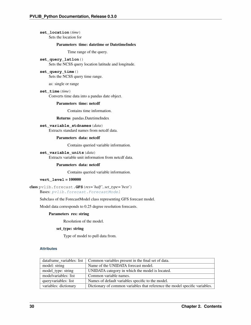
class pvlib.forecast.GFS(res=’half’, set_type=’best’)Bases: pvlib.forecast.ForecastModel

Subclass of the ForecastModel class representing GFS forecast model.

Model data corresponds to 0.25 degree resolution forecasts.

Parameters res: string

Resolution of the model.

set_type: string

Type of model to pull data from.

Attributes

dataframe_variables: list Common variables present in the final set of data.model: string Name of the UNIDATA forecast model.model_type: string UNIDATA category in which the model is located.modelvariables: list Common variable names.queryvariables: list Names of default variables specific to the model.variables: dictionary Dictionary of common variables that reference the model specific variables.



class pvlib.forecast.HRRR(set_type=’best’)Bases: pvlib.forecast.ForecastModel

Subclass of the ForecastModel class representing HRRR forecast model.

Model data corresponds to NCEP HRRR CONUS 2.5km resolution forecasts.

Parameters set_type: string


Attributes


class pvlib.forecast.HRRR_ESRL(set_type=’best’)Bases: pvlib.forecast.ForecastModel

Subclass of the ForecastModel class representing NOAA/GSD/ESRL’s HRRR forecast model. This is not anoperational product.

Model data corresponds to NOAA/GSD/ESRL HRRR CONUS 3km resolution surface forecasts.



Attributes


class pvlib.forecast.NAM(set_type=’best’)Bases: pvlib.forecast.ForecastModel

Subclass of the ForecastModel class representing NAM forecast model.

Model data corresponds to NAM CONUS 12km resolution forecasts from CONDUIT.



2.4. Modules 31


Attributes


class pvlib.forecast.NDFD(set_type=’best’)Bases: pvlib.forecast.ForecastModel

Subclass of the ForecastModel class representing NDFD forecast model.

Model data corresponds to NWS CONUS CONDUIT forecasts.



Attributes


class pvlib.forecast.RAP(set_type=’best’)Bases: pvlib.forecast.ForecastModel

Subclass of the ForecastModel class representing RAP forecast model.

Model data corresponds to Rapid Refresh CONUS 20km resolution forecasts.



Attributes


2.4.4 irradiance module

The irradiance module contains functions for modeling global horizontal irradiance, direct normal irradiance,diffuse horizontal irradiance, and total irradiance under various conditions.



pvlib.irradiance.aoi(surface_tilt, surface_azimuth, solar_zenith, solar_azimuth)Calculates the angle of incidence of the solar vector on a surface. This is the angle between the solar vector andthe surface normal.

Input all angles in degrees.

Parameters surface_tilt : float or Series.

Panel tilt from horizontal.

surface_azimuth : float or Series.

Panel azimuth from north.

solar_zenith : float or Series.

Solar zenith angle.

solar_azimuth : float or Series.

Solar azimuth angle.

Returns float or Series. Angle of incidence in degrees.

pvlib.irradiance.aoi_projection(surface_tilt, surface_azimuth, solar_zenith, solar_azimuth)Calculates the dot product of the solar vector and the surface normal.







Solar zenith angle.



Returns float or Series. Dot product of panel normal and solar angle.

pvlib.irradiance.beam_component(surface_tilt, surface_azimuth, solar_zenith, solar_azimuth,dni)

Calculates the beam component of the plane of array irradiance.






Solar zenith angle.



dni : float or Series

Direct Normal Irradiance

2.4. Modules 33


Returns Series

pvlib.irradiance.cloudy_day_check(zenith, cloud_prct, pressure=101325.0)Determines if the sky is overcast.

Returns logical: bool

Is the sky is overcast.

References


pvlib.irradiance.dirint(ghi, zenith, times, pressure=101325, use_delta_kt_prime=True,temp_dew=None)

Determine DNI from GHI using the DIRINT modification of the DISC model.

Implements the modified DISC model known as “DIRINT” introduced in [1]. DIRINT predicts direct normalirradiance (DNI) from measured global horizontal irradiance (GHI). DIRINT improves upon the DISC modelby using time-series GHI data and dew point temperature information. The effectiveness of the DIRINT modelimproves with each piece of information provided.

Parameters ghi : pd.Series

Global horizontal irradiance in W/m^2.

zenith : pd.Series

True (not refraction-corrected) zenith angles in decimal degrees. If Z is a vector it mustbe of the same size as all other vector inputs. Z must be >=0 and <=180.

times : DatetimeIndex

pressure : float or pd.Series

The site pressure in Pascal. Pressure may be measured or an average pressure may becalculated from site altitude.

use_delta_kt_prime : bool

Indicates if the user would like to utilize the time-series nature of the GHI measure-ments. A value of False will not use the time-series improvements, any other numericvalue will use time-series improvements. It is recommended that time-series data onlybe used if the time between measured data points is less than 1.5 hours. If none of theinput arguments are vectors, then time-series improvements are not used (because it’snot a time-series).

temp_dew : None, float, or pd.Series

Surface dew point temperatures, in degrees C. Values of temp_dew may be numeric orNaN. Any single time period point with a DewPtTemp=NaN does not have dew pointimprovements applied. If DewPtTemp is not provided, then dew point improvementsare not applied.

Returns dni : pd.Series.

The modeled direct normal irradiance in W/m^2 provided by the DIRINT model.



References

[1] Perez, R., P. Ineichen, E. Maxwell, R. Seals and A. Zelenka, (1992). “Dynamic Global-to-Direct IrradianceConversion Models”. ASHRAE Transactions-Research Series, pp. 354-369

[2] Maxwell, E. L., “A Quasi-Physical Model for Converting Hourly Global Horizontal to Direct Normal Inso-lation”, Technical Report No. SERI/TR-215-3087, Golden, CO: Solar Energy Research Institute, 1987.

DIRINT model requires time series data (ie. one of the inputs must be a vector of length >2.

pvlib.irradiance.disc(ghi, zenith, times, pressure=101325)Estimate Direct Normal Irradiance from Global Horizontal Irradiance using the DISC model.

The DISC algorithm converts global horizontal irradiance to direct normal irradiance through empirical rela-tionships between the global and direct clearness indices.

Parameters ghi : Series


solar_zenith : Series

True (not refraction - corrected) solar zenith angles in decimal degrees.

times : DatetimeIndex

pressure : float or Series

Site pressure in Pascal.

Returns DataFrame with the following keys:

• dni: The modeled direct normal irradiance in W/m^2 provided by the Direct InsolationSimulation Code (DISC) model.

• kt: Ratio of global to extraterrestrial irradiance on a horizontal plane.

• airmass: Airmass

See also:

atmosphere.alt2pres, dirint

References

[1] Maxwell, E. L., “A Quasi-Physical Model for Converting Hourly Global Horizontal to Direct Normal Inso-lation”, Technical Report No. SERI/TR-215-3087, Golden, CO: Solar Energy Research Institute, 1987.

[2] J.W. “Fourier series representation of the position of the sun”. Found at: http://www.mail-archive.com/[email protected]/msg01050.html on January 12, 2012

pvlib.irradiance.extraradiation(datetime_or_doy, solar_constant=1366.1, method=’spencer’)Determine extraterrestrial radiation from day of year.

Parameters datetime_or_doy : int, float, array, pd.DatetimeIndex

Day of year, array of days of year e.g. pd.DatetimeIndex.dayofyear, orpd.DatetimeIndex.

solar_constant : float

The solar constant.

method : string

2.4. Modules 35

http://www.mail-archive.com/[email protected]/msg01050.html

http://www.mail-archive.com/[email protected]/msg01050.html


The method by which the ET radiation should be calculated. Options include’pyephem’, ’spencer’, ’asce’.

Returns float or Series

The extraterrestrial radiation present in watts per square meter on a surface which isnormal to the sun. Ea is of the same size as the input doy.

‘pyephem’ always returns a series.

See also:

pvlib.clearsky.disc

Notes

The Spencer method contains a minus sign discrepancy between equation 12 of [1]. It’s unclear what the correctformula is.

References

[1] M. Reno, C. Hansen, and J. Stein, “Global Horizontal Irradiance Clear Sky Models: Implementation andAnalysis”, Sandia National Laboratories, SAND2012-2389, 2012.

[2] <http://solardat.uoregon.edu/SolarRadiationBasics.html>, Eqs. SR1 and SR2

[3] Partridge, G. W. and Platt, C. M. R. 1976. Radiative Processes in Meteorology and Climatology.

[4] Duffie, J. A. and Beckman, W. A. 1991. Solar Engineering of Thermal Processes, 2nd edn. J. Wiley andSons, New York.

pvlib.irradiance.globalinplane(aoi, dni, poa_sky_diffuse, poa_ground_diffuse)Determine the three components on in-plane irradiance

Combines in-plane irradaince compoents from the chosen diffuse translation, ground reflection and beam irra-diance algorithms into the total in-plane irradiance.

Parameters aoi : float or Series

Angle of incidence of solar rays with respect to the module surface, from aoi().


Direct normal irradiance (W/m^2), as measured from a TMY file or calculated with aclearsky model.

poa_sky_diffuse : float or Series

Diffuse irradiance (W/m^2) in the plane of the modules, as calculated by a diffuse irra-diance translation function

poa_ground_diffuse : float or Series

Ground reflected irradiance (W/m^2) in the plane of the modules, as calculated by analbedo model (eg. grounddiffuse())

Returns DataFrame with the following keys:

• poa_global : Total in-plane irradiance (W/m^2)

• poa_direct : Total in-plane beam irradiance (W/m^2)

• poa_diffuse : Total in-plane diffuse irradiance (W/m^2)


http://solardat.uoregon.edu/SolarRadiationBasics.html


Notes

Negative beam irradiation due to aoi > 90∘ or AOI < 0∘ is set to zero.

pvlib.irradiance.grounddiffuse(surface_tilt, ghi, albedo=0.25, surface_type=None)Estimate diffuse irradiance from ground reflections given irradiance, albedo, and surface tilt

Function to determine the portion of irradiance on a tilted surface due to ground reflections. Any of the inputsmay be DataFrames or scalars.

Parameters surface_tilt : float or DataFrame

Surface tilt angles in decimal degrees. SurfTilt must be >=0 and <=180. The tilt angleis defined as degrees from horizontal (e.g. surface facing up = 0, surface facing horizon= 90).

ghi : float or DataFrame


albedo : float or DataFrame

Ground reflectance, typically 0.1-0.4 for surfaces on Earth (land), may increase oversnow, ice, etc. May also be known as the reflection coefficient. Must be >=0 and <=1.Will be overridden if surface_type is supplied.

surface_type: None or string in

’urban’, ’grass’, ’fresh grass’, ’snow’, ’fresh snow’,’asphalt’, ’concrete’, ’aluminum’, ’copper’, ’freshsteel’, ’dirty steel’. Overrides albedo.

Returns float or DataFrame

Ground reflected irradiances in W/m^2.

References

[1] Loutzenhiser P.G. et. al. “Empirical validation of models to compute solar irradiance on inclined surfacesfor building energy simulation” 2007, Solar Energy vol. 81. pp. 254-267.

The calculation is the last term of equations 3, 4, 7, 8, 10, 11, and 12.

[2] albedos from: http://pvpmc.org/modeling-steps/incident-irradiance/plane-of-array-poa-irradiance/calculating-poa-irradiance/poa-ground-reflected/albedo/

and http://en.wikipedia.org/wiki/Albedo

pvlib.irradiance.haydavies(surface_tilt, surface_azimuth, dhi, dni, dni_extra, solar_zenith=None,solar_azimuth=None, projection_ratio=None)

Determine diffuse irradiance from the sky on a tilted surface using Hay & Davies’ 1980 model

𝐼𝑑 = 𝐷𝐻𝐼(𝐴𝑅𝑏 + (1−𝐴)(1 + cos𝛽

2))

Hay and Davies’ 1980 model determines the diffuse irradiance from the sky (ground reflected irradiance isnot included in this algorithm) on a tilted surface using the surface tilt angle, surface azimuth angle, diffusehorizontal irradiance, direct normal irradiance, extraterrestrial irradiance, sun zenith angle, and sun azimuthangle.

Parameters surface_tilt : float or Series

2.4. Modules 37

http://pvpmc.org/modeling-steps/incident-irradiance/plane-of-array-poa-irradiance/calculating-poa-irradiance/poa-ground-reflected/albedo/

http://pvpmc.org/modeling-steps/incident-irradiance/plane-of-array-poa-irradiance/calculating-poa-irradiance/poa-ground-reflected/albedo/

http://en.wikipedia.org/wiki/Albedo


Surface tilt angles in decimal degrees. The tilt angle is defined as degrees from horizon-tal (e.g. surface facing up = 0, surface facing horizon = 90)

surface_azimuth : float or Series

Surface azimuth angles in decimal degrees. The azimuth convention is defined as de-grees east of north (e.g. North=0, South=180, East=90, West=270).

dhi : float or Series

Diffuse horizontal irradiance in W/m^2.


Direct normal irradiance in W/m^2.

dni_extra : float or Series

Extraterrestrial normal irradiance in W/m^2.

solar_zenith : None, float or Series

Solar apparent (refraction-corrected) zenith angles in decimal degrees. Must supplysolar_zenith and solar_azimuth or supply projection_ratio.

solar_azimuth : None, float or Series

Solar azimuth angles in decimal degrees. Must supply solar_zenith andsolar_azimuth or supply projection_ratio.

projection_ratio : None, float or Series

Ratio of angle of incidence projection to solar zenith angle projection. Must supplysolar_zenith and solar_azimuth or supply projection_ratio.

Returns sky_diffuse : float or Series

The diffuse component of the solar radiation on an arbitrarily tilted surface definedby the Perez model as given in reference [3]. Does not include the ground reflectedirradiance or the irradiance due to the beam.

References

[1] Loutzenhiser P.G. et. al. “Empirical validation of models to compute solar irradiance on inclined surfacesfor building energy simulation” 2007, Solar Energy vol. 81. pp. 254-267

[2] Hay, J.E., Davies, J.A., 1980. Calculations of the solar radiation incident on an inclined surface. In: Hay,J.E., Won, T.K. (Eds.), Proc. of First Canadian Solar Radiation Data Workshop, 59. Ministry of Supply andServices, Canada.

pvlib.irradiance.isotropic(surface_tilt, dhi)Determine diffuse irradiance from the sky on a tilted surface using the isotropic sky model.

𝐼𝑑 = 𝐷𝐻𝐼1 + cos𝛽

2

Hottel and Woertz’s model treats the sky as a uniform source of diffuse irradiance. Thus the diffuse irradiancefrom the sky (ground reflected irradiance is not included in this algorithm) on a tilted surface can be found fromthe diffuse horizontal irradiance and the tilt angle of the surface.




Surface tilt angle in decimal degrees. surface_tilt must be >=0 and <=180. The tilt angleis defined as degrees from horizontal (e.g. surface facing up = 0, surface facing horizon= 90)


Diffuse horizontal irradiance in W/m^2. DHI must be >=0.


The diffuse component of the solar radiation on an

arbitrarily tilted surface defined by the isotropic sky model as

given in Loutzenhiser et. al (2007) equation 3.

SkyDiffuse is the diffuse component ONLY and does not include the ground

reflected irradiance or the irradiance due to the beam.

SkyDiffuse is a column vector vector with a number of elements equal to

the input vector(s).

References


[2] Hottel, H.C., Woertz, B.B., 1942. Evaluation of flat-plate solar heat collector. Trans. ASME 64, 91.

pvlib.irradiance.king(surface_tilt, dhi, ghi, solar_zenith)Determine diffuse irradiance from the sky on a tilted surface using the King model.

King’s model determines the diffuse irradiance from the sky (ground reflected irradiance is not included inthis algorithm) on a tilted surface using the surface tilt angle, diffuse horizontal irradiance, global horizontalirradiance, and sun zenith angle. Note that this model is not well documented and has not been published in anyfashion (as of January 2012).




Diffuse horizontal irradiance in W/m^2.

ghi : float or Series


solar_zenith : float or Series

Apparent (refraction-corrected) zenith angles in decimal degrees.

Returns poa_sky_diffuse : float or Series

The diffuse component of the solar radiation on an arbitrarily tilted surface as given bya model developed by David L. King at Sandia National Laboratories.

pvlib.irradiance.klucher(surface_tilt, surface_azimuth, dhi, ghi, solar_zenith, solar_azimuth)Determine diffuse irradiance from the sky on a tilted surface using Klucher’s 1979 model

𝐼𝑑 = 𝐷𝐻𝐼1 + cos𝛽

2(1 + 𝐹 ′ sin3(𝛽/2))(1 + 𝐹 ′ cos2 𝜃 sin3 𝜃𝑧)

2.4. Modules 39


where

𝐹 ′ = 1− (𝐼𝑑0/𝐺𝐻𝐼)

Klucher’s 1979 model determines the diffuse irradiance from the sky (ground reflected irradiance is not includedin this algorithm) on a tilted surface using the surface tilt angle, surface azimuth angle, diffuse horizontal irradi-ance, direct normal irradiance, global horizontal irradiance, extraterrestrial irradiance, sun zenith angle, and sunazimuth angle.


Surface tilt angles in decimal degrees. surface_tilt must be >=0 and <=180. The tiltangle is defined as degrees from horizontal (e.g. surface facing up = 0, surface facinghorizon = 90)


Surface azimuth angles in decimal degrees. surface_azimuth must be >=0 and <=360.The Azimuth convention is defined as degrees east of north (e.g. North = 0, South=180East = 90, West = 270).


diffuse horizontal irradiance in W/m^2. DHI must be >=0.


Global irradiance in W/m^2. DNI must be >=0.


apparent (refraction-corrected) zenith angles in decimal degrees. solar_zenith must be>=0 and <=180.

solar_azimuth : float or Series

Sun azimuth angles in decimal degrees. solar_azimuth must be >=0 and <=360. TheAzimuth convention is defined as degrees east of north (e.g. North = 0, East = 90, West= 270).

Returns float or Series.

The diffuse component of the solar radiation on an

arbitrarily tilted surface defined by the Klucher model as given in

Loutzenhiser et. al (2007) equation 4.

SkyDiffuse is the diffuse component ONLY and does not include the ground

reflected irradiance or the irradiance due to the beam.

SkyDiffuse is a column vector vector with a number of elements equal to

the input vector(s).

References


[2] Klucher, T.M., 1979. Evaluation of models to predict insolation on tilted surfaces. Solar Energy 23 (2),111-114.



pvlib.irradiance.liujordan(zenith, cloud_prct, pressure=101325.0)Determine DNI, DHI, GHI from extraterrestrial flux, transmittance, and optical air mass number.

Liu and Jordan, 1960, developed a simplified direct radiation model. DHI is from an empirical equation fordiffuse radiation from Liu and Jordan, 1960.

Parameters zenith : pd.Series

True (not refraction-corrected) zenith angles in decimal degrees. If Z is a vector it mustbe of the same size as all other vector inputs. Z must be >=0 and <=180.

cloud_prct : integer or float

Cloud coverage in percentage, %.

Returns Pandas.DataFrame

Modeled direct normal irradiance, direct horizontal irradiance, and global horizontalirradiance in W/m^2

References


[2] Liu, B. Y., R. C. Jordan, (1960). “The interrelationship and characteristic distribution of direct, diffuse, andtotal solar radiation”. Solar Energy 4:1-19

pvlib.irradiance.perez(surface_tilt, surface_azimuth, dhi, dni, dni_extra, solar_zenith, so-lar_azimuth, airmass, modelt=’allsitescomposite1990’)

Determine diffuse irradiance from the sky on a tilted surface using one of the Perez models.

Perez models determine the diffuse irradiance from the sky (ground reflected irradiance is not included in thisalgorithm) on a tilted surface using the surface tilt angle, surface azimuth angle, diffuse horizontal irradiance, di-rect normal irradiance, extraterrestrial irradiance, sun zenith angle, sun azimuth angle, and relative (not pressure-corrected) airmass. Optionally a selector may be used to use any of Perez’s model coefficient sets.


Surface tilt angles in decimal degrees. surface_tilt must be >=0 and <=180. The tiltangle is defined as degrees from horizontal (e.g. surface facing up = 0, surface facinghorizon = 90)


Surface azimuth angles in decimal degrees. surface_azimuth must be >=0 and <=360.The Azimuth convention is defined as degrees east of north (e.g. North = 0, South=180East = 90, West = 270).


Diffuse horizontal irradiance in W/m^2. DHI must be >=0.


Direct normal irradiance in W/m^2. DNI must be >=0.


Extraterrestrial normal irradiance in W/m^2.


2.4. Modules 41


apparent (refraction-corrected) zenith angles in decimal degrees. solar_zenith must be>=0 and <=180.

solar_azimuth : float or Series

Sun azimuth angles in decimal degrees. solar_azimuth must be >=0 and <=360. TheAzimuth convention is defined as degrees east of north (e.g. North = 0, East = 90, West= 270).

airmass : float or Series

relative (not pressure-corrected) airmass values. If AM is a DataFrame it must be of thesame size as all other DataFrame inputs. AM must be >=0 (careful using the 1/sec(z)model of AM generation)

model : string (optional, default=’allsitescomposite1990’)

A string which selects the desired set of Perez coefficients. If model is not provided asan input, the default, ‘1990’ will be used. All possible model selections are:

• ‘1990’

• ‘allsitescomposite1990’ (same as ‘1990’)

• ‘allsitescomposite1988’

• ‘sandiacomposite1988’

• ‘usacomposite1988’

• ‘france1988’

• ‘phoenix1988’

• ‘elmonte1988’

• ‘osage1988’

• ‘albuquerque1988’

• ‘capecanaveral1988’

• ‘albany1988’


The diffuse component of the solar radiation on an arbitrarily tilted surface defined bythe Perez model as given in reference [3]. SkyDiffuse is the diffuse component ONLYand does not include the ground reflected irradiance or the irradiance due to the beam.

References


[2] Perez, R., Seals, R., Ineichen, P., Stewart, R., Menicucci, D., 1987. A new simplified version of the Perezdiffuse irradiance model for tilted surfaces. Solar Energy 39(3), 221-232.

[3] Perez, R., Ineichen, P., Seals, R., Michalsky, J., Stewart, R., 1990. Modeling daylight availability andirradiance components from direct and global irradiance. Solar Energy 44 (5), 271-289.

[4] Perez, R. et. al 1988. “The Development and Verification of the Perez Diffuse Radiation Model”. SAND88-7030



pvlib.irradiance.poa_horizontal_ratio(surface_tilt, surface_azimuth, solar_zenith, so-lar_azimuth)

Calculates the ratio of the beam components of the plane of array irradiance and the horizontal irradiance.







Solar zenith angle.



Returns float or Series. Ratio of the plane of array irradiance to the

horizontal plane irradiance

pvlib.irradiance.reindl(surface_tilt, surface_azimuth, dhi, dni, ghi, dni_extra, solar_zenith, so-lar_azimuth)

Determine diffuse irradiance from the sky on a tilted surface using Reindl’s 1990 model

𝐼𝑑 = 𝐷𝐻𝐼(𝐴𝑅𝑏 + (1−𝐴)(1 + cos𝛽

2)(1 +

√︂𝐼ℎ𝑏𝐼ℎ

sin3(𝛽/2)))

Reindl’s 1990 model determines the diffuse irradiance from the sky (ground reflected irradiance is not includedin this algorithm) on a tilted surface using the surface tilt angle, surface azimuth angle, diffuse horizontal irradi-ance, direct normal irradiance, global horizontal irradiance, extraterrestrial irradiance, sun zenith angle, and sunazimuth angle.




Surface azimuth angles in decimal degrees. The Azimuth convention is defined as de-grees east of north (e.g. North = 0, South=180 East = 90, West = 270).

dhi : float or Series.

diffuse horizontal irradiance in W/m^2.

dni : float or Series.

direct normal irradiance in W/m^2.

ghi: float or Series.

Global irradiance in W/m^2.

dni_extra : float or Series.

extraterrestrial normal irradiance in W/m^2.


apparent (refraction-corrected) zenith angles in decimal degrees.

2.4. Modules 43



Sun azimuth angles in decimal degrees. The Azimuth convention is defined as degreeseast of north (e.g. North = 0, East = 90, West = 270).

Returns poa_sky_diffuse : float or Series.

The diffuse component of the solar radiation on an arbitrarily tilted surface defined bythe Reindl model as given in Loutzenhiser et. al (2007) equation 8. SkyDiffuse is thediffuse component ONLY and does not include the ground reflected irradiance or theirradiance due to the beam. SkyDiffuse is a column vector vector with a number ofelements equal to the input vector(s).

Notes

The poa_sky_diffuse calculation is generated from the Loutzenhiser et al. (2007) paper, equation 8. Note thatI have removed the beam and ground reflectance portion of the equation and this generates ONLY the diffuseradiation from the sky and circumsolar, so the form of the equation varies slightly from equation 8.

References


[2] Reindl, D.T., Beckmann, W.A., Duffie, J.A., 1990a. Diffuse fraction correlations. Solar Energy 45(1), 1-7.

[3] Reindl, D.T., Beckmann, W.A., Duffie, J.A., 1990b. Evaluation of hourly tilted surface radiation models.Solar Energy 45(1), 9-17.

pvlib.irradiance.total_irrad(surface_tilt, surface_azimuth, solar_zenith, solar_azimuth,dni, ghi, dhi, dni_extra=None, airmass=None,albedo=0.25, surface_type=None, model=’isotropic’,model_perez=’allsitescomposite1990’)

Determine diffuse irradiance from the sky on a tilted surface.

𝐼𝑡𝑜𝑡 = 𝐼𝑏𝑒𝑎𝑚 + 𝐼𝑠𝑘𝑦 + 𝐼𝑔𝑟𝑜𝑢𝑛𝑑






Solar zenith angle.




Direct Normal Irradiance


Global horizontal irradiance




Diffuse horizontal irradiance


Extraterrestrial direct normal irradiance

airmass : float or Series

Airmass

albedo : float

Surface albedo

surface_type : String

Surface type. See grounddiffuse.

model : String

Irradiance model.

model_perez : String

See perez.

Returns DataFrame with columns ’total’, ’beam’, ’sky’, ’ground’.

References


2.4.5 location module

This module contains the Location class.

class pvlib.location.Location(latitude, longitude, tz=’US/Mountain’, altitude=100, name=None)Bases: object

Location objects are convenient containers for latitude, longitude, timezone, and altitude data associated with aparticular geographic location. You can also assign a name to a location object.

Location objects have two timezone attributes:

•location.tz is a IANA timezone string.

•location.pytz is a pytz timezone object.

Location objects support the print method.

Parameters latitude : float.

Positive is north of the equator. Use decimal degrees notation.

longitude : float.

Positive is east of the prime meridian. Use decimal degrees notation.

tz : string or pytz.timezone.

See http://en.wikipedia.org/wiki/List_of_tz_database_time_zones for a list of valid timezones. pytz.timezone objects will be converted to strings.

alitude : float.

2.4. Modules 45

http://en.wikipedia.org/wiki/List_of_tz_database_time_zones


Altitude from sea level in meters.

name : None or string.

Sets the name attribute of the Location object.

2.4.6 pvsystem module

The pvsystem module contains functions for modeling the output and performance of PV modules and inverters.

pvlib.pvsystem.ashraeiam(b, aoi)Determine the incidence angle modifier using the ASHRAE transmission model.

ashraeiam calculates the incidence angle modifier as developed in [1], and adopted by ASHRAE (AmericanSociety of Heating, Refrigeration, and Air Conditioning Engineers) [2]. The model has been used by modelprograms such as PVSyst [3].

Note: For incident angles near 90 degrees, this model has a discontinuity which has been addressed in thisfunction.

Parameters b : float

A parameter to adjust the modifier as a function of angle of incidence. Typical valuesare on the order of 0.05 [3].

aoi : Series

The angle of incidence between the module normal vector and the sun-beam vector indegrees.

Returns IAM : Series

The incident angle modifier calculated as 1-b*(sec(aoi)-1) as described in [2,3].

Returns nan for all abs(aoi) >= 90 and for all IAM values that would be less than 0.

See also:

irradiance.aoi, physicaliam

References

[1] Souka A.F., Safwat H.H., “Determindation of the optimum orientations for the double exposure flat-platecollector and its reflections”. Solar Energy vol .10, pp 170-174. 1966.

[2] ASHRAE standard 93-77

[3] PVsyst Contextual Help. http://files.pvsyst.com/help/index.html?iam_loss.htm retrieved on September 10,2012

pvlib.pvsystem.calcparams_desoto(poa_global, temp_cell, alpha_isc, module_parameters,EgRef, dEgdT, M=1, irrad_ref=1000, temp_ref=25)

Applies the temperature and irradiance corrections to inputs for singlediode.

Applies the temperature and irradiance corrections to the IL, I0, Rs, Rsh, and a parameters at reference condi-tions (IL_ref, I0_ref, etc.) according to the De Soto et. al description given in [1]. The results of this correctionprocedure may be used in a single diode model to determine IV curves at irradiance = S, cell temperature =Tcell.

Parameters poa_global : float or Series

The irradiance (in W/m^2) absorbed by the module.


http://files.pvsyst.com/help/index.html?iam_loss.htm


temp_cell : float or Series

The average cell temperature of cells within a module in C.

alpha_isc : float

The short-circuit current temperature coefficient of the module in units of 1/C.

module_parameters : dict

Parameters describing PV module performance at reference conditions according toDeSoto’s paper. Parameters may be generated or found by lookup. For ease of use,retrieve_sam can automatically generate a dict based on the most recent SAM CECmodule database. The module_parameters dict must contain the following 5 fields:

• a_ref - modified diode ideality factor parameter at reference conditions (units of eV),a_ref can be calculated from the usual diode ideality factor (n), number of cells inseries (Ns), and cell temperature (Tcell) per equation (2) in [1].

• I_L_ref - Light-generated current (or photocurrent) in amperes at reference condi-tions. This value is referred to as Iph in some literature.

• I_o_ref - diode reverse saturation current in amperes, under reference conditions.

• R_sh_ref - shunt resistance under reference conditions (ohms).

• R_s - series resistance under reference conditions (ohms).

EgRef : float

The energy bandgap at reference temperature (in eV). 1.121 eV for silicon. EgRef mustbe >0.

dEgdT : float

The temperature dependence of the energy bandgap at SRC (in 1/C). May be either ascalar value (e.g. -0.0002677 as in [1]) or a DataFrame of dEgdT values correspondingto each input condition (this may be useful if dEgdT is a function of temperature).

M : float or Series (optional, default=1)

An optional airmass modifier, if omitted, M is given a value of 1, which assumes abso-lute (pressure corrected) airmass = 1.5. In this code, M is equal to M/Mref as describedin [1] (i.e. Mref is assumed to be 1). Source [1] suggests that an appropriate value forM as a function absolute airmass (AMa) may be:

>>> M = np.polyval([-0.000126, 0.002816, -0.024459, 0.086257, 0.918093],... AMa)

M may be a Series.

irrad_ref : float (optional, default=1000)

Reference irradiance in W/m^2.

temp_ref : float (optional, default=25)

Reference cell temperature in C.

Returns Tuple of the following results:

photocurrent : float or Series

Light-generated current in amperes at irradiance=S and cell temperature=Tcell.

saturation_current : float or Series

2.4. Modules 47


Diode saturation curent in amperes at irradiance S and cell temperature Tcell.

resistance_series : float

Series resistance in ohms at irradiance S and cell temperature Tcell.

resistance_shunt : float or Series

Shunt resistance in ohms at irradiance S and cell temperature Tcell.

nNsVth : float or Series

Modified diode ideality factor at irradiance S and cell temperature Tcell. Note that insource [1] nNsVth = a (equation 2). nNsVth is the product of the usual diode idealityfactor (n), the number of series-connected cells in the module (Ns), and the thermalvoltage of a cell in the module (Vth) at a cell temperature of Tcell.

See also:

sapm, sapm_celltemp, singlediode, retrieve_sam

Notes

If the reference parameters in the ModuleParameters struct are read from a database or library of parameters (e.g.System Advisor Model), it is important to use the same EgRef and dEgdT values that were used to generate thereference parameters, regardless of the actual bandgap characteristics of the semiconductor. For example, in thecase of the System Advisor Model library, created as described in [3], EgRef and dEgdT for all modules were1.121 and -0.0002677, respectively.

This table of reference bandgap energies (EgRef), bandgap energy temperature dependence (dEgdT), and “typi-cal” airmass response (M) is provided purely as reference to those who may generate their own reference moduleparameters (a_ref, IL_ref, I0_ref, etc.) based upon the various PV semiconductors. Again, we stress the impor-tance of using identical EgRef and dEgdT when generation reference parameters and modifying the referenceparameters (for irradiance, temperature, and airmass) per DeSoto’s equations.

Silicon (Si):

• EgRef = 1.121

• dEgdT = -0.0002677

>>> M = np.polyval([-1.26E-4, 2.816E-3, -0.024459, 0.086257, 0.918093],... AMa)

Source: [1]

Cadmium Telluride (CdTe):

• EgRef = 1.475

• dEgdT = -0.0003

>>> M = np.polyval([-2.46E-5, 9.607E-4, -0.0134, 0.0716, 0.9196],... AMa)

Source: [4]

Copper Indium diSelenide (CIS):

• EgRef = 1.010

• dEgdT = -0.00011



>>> M = np.polyval([-3.74E-5, 0.00125, -0.01462, 0.0718, 0.9210],... AMa)

Source: [4]

Copper Indium Gallium diSelenide (CIGS):

• EgRef = 1.15

• dEgdT = ????

>>> M = np.polyval([-9.07E-5, 0.0022, -0.0202, 0.0652, 0.9417],... AMa)

Source: Wikipedia

Gallium Arsenide (GaAs):

• EgRef = 1.424

• dEgdT = -0.000433

• M = unknown

Source: [4]

References

[1] W. De Soto et al., “Improvement and validation of a model for photovoltaic array performance”, SolarEnergy, vol 80, pp. 78-88, 2006.

[2] System Advisor Model web page. https://sam.nrel.gov.

[3] A. Dobos, “An Improved Coefficient Calculator for the California Energy Commission 6 Parameter Photo-voltaic Module Model”, Journal of Solar Energy Engineering, vol 134, 2012.

[4] O. Madelung, “Semiconductors: Data Handbook, 3rd ed.” ISBN 3-540-40488-0

pvlib.pvsystem.i_from_v(resistance_shunt, resistance_series, nNsVth, voltage, saturation_current,photocurrent)

Calculates current from voltage per Eq 2 Jain and Kapoor 2004 [1].

Parameters resistance_series : float or Series

Series resistance in ohms under desired IV curve conditions. Often abbreviated Rs.


Shunt resistance in ohms under desired IV curve conditions. Often abbreviated Rsh.


Diode saturation current in amperes under desired IV curve conditions. Often abbrevi-ated I_0.


The product of three components. 1) The usual diode ideal factor (n), 2) the num-ber of cells in series (Ns), and 3) the cell thermal voltage under the desired IV curveconditions (Vth). The thermal voltage of the cell (in volts) may be calculated ask*temp_cell/q, where k is Boltzmann’s constant (J/K), temp_cell is the temper-ature of the p-n junction in Kelvin, and q is the charge of an electron (coulombs).

2.4. Modules 49

https://sam.nrel.gov



Light-generated current (photocurrent) in amperes under desired IV curve conditions.Often abbreviated I_L.

Returns current : np.array

References

[1] A. Jain, A. Kapoor, “Exact analytical solutions of the parameters of real solar cells using Lambert W-function”, Solar Energy Materials and Solar Cells, 81 (2004) 269-277.

pvlib.pvsystem.physicaliam(K, L, n, aoi)Determine the incidence angle modifier using refractive index, glazing thickness, and extinction coefficient

physicaliam calculates the incidence angle modifier as described in De Soto et al. “Improvement and validationof a model for photovoltaic array performance”, section 3. The calculation is based upon a physical model ofabsorbtion and transmission through a cover. Required information includes, incident angle, cover extinctioncoefficient, cover thickness

Note: The authors of this function believe that eqn. 14 in [1] is incorrect. This function uses the followingequation in its place: theta_r = arcsin(1/n * sin(theta))

Parameters K : float

The glazing extinction coefficient in units of 1/meters. Reference [1] indicates that avalue of 4 is reasonable for “water white” glass. K must be a numeric scalar or vectorwith all values >=0. If K is a vector, it must be the same size as all other input vectors.

L : float

The glazing thickness in units of meters. Reference [1] indicates that 0.002 meters (2mm) is reasonable for most glass-covered PV panels. L must be a numeric scalar orvector with all values >=0. If L is a vector, it must be the same size as all other inputvectors.

n : float

The effective index of refraction (unitless). Reference [1] indicates that a value of 1.526is acceptable for glass. n must be a numeric scalar or vector with all values >=0. If n isa vector, it must be the same size as all other input vectors.

aoi : Series

The angle of incidence between the module normal vector and the sun-beam vector indegrees.

Returns IAM : float or Series

The incident angle modifier as specified in eqns. 14-16 of [1]. IAM is a column vectorwith the same number of elements as the largest input vector.

Theta must be a numeric scalar or vector. For any values of theta where abs(aoi)>90,IAM is set to 0. For any values of aoi where -90 < aoi < 0, theta is set to abs(aoi) andevaluated.

See also:

getaoi, ephemeris, spa, ashraeiam



References

[1] W. De Soto et al., “Improvement and validation of a model for photovoltaic array performance”, SolarEnergy, vol 80, pp. 78-88, 2006.

[2] Duffie, John A. & Beckman, William A.. (2006). Solar Engineering of Thermal Processes, third edition.[Books24x7 version] Available from http://common.books24x7.com/toc.aspx?bookid=17160.

pvlib.pvsystem.retrieve_sam(name=None, samfile=None)Retrieve latest module and inverter info from SAM website.

This function will retrieve either:

•CEC module database

•Sandia Module database

•CEC Inverter database

and return it as a pandas dataframe.

Parameters name : String

Name can be one of:

• ‘CECMod’ - returns the CEC module database

• ‘CECInverter’ - returns the CEC Inverter database

• ‘SandiaInverter’ - returns the CEC Inverter database (CEC is only current inverter dbavailable; tag kept for backwards compatibility)

• ‘SandiaMod’ - returns the Sandia Module database

samfile : String

Absolute path to the location of local versions of the SAM file. If file is specified, thelatest versions of the SAM database will not be downloaded. The selected file must bein .csv format.

If set to ‘select’, a dialogue will open allowing the user to navigate to the appropriatepage.

Returns A DataFrame containing all the elements of the desired database.

Each column represents a module or inverter, and a specific dataset

can be retrieved by the command

Examples

>>> from pvlib import pvsystem>>> invdb = pvsystem.retrieve_sam(name='CECInverter')>>> inverter = invdb.AE_Solar_Energy__AE6_0__277V__277V__CEC_2012_>>> inverterVac 277.000000Paco 6000.000000Pdco 6165.670000Vdco 361.123000Pso 36.792300C0 -0.000002C1 -0.000047C2 -0.001861

2.4. Modules 51

http://common.books24x7.com/toc.aspx?bookid=17160


C3 0.000721Pnt 0.070000Vdcmax 600.000000Idcmax 32.000000Mppt_low 200.000000Mppt_high 500.000000Name: AE_Solar_Energy__AE6_0__277V__277V__CEC_2012_, dtype: float64

pvlib.pvsystem.sapm(module, poa_direct, poa_diffuse, temp_cell, airmass_absolute, aoi)The Sandia PV Array Performance Model (SAPM) generates 5 points on a PV module’s I-V curve (Voc, Isc, Ix,Ixx, Vmp/Imp) according to SAND2004-3535. Assumes a reference cell temperature of 25 C.

Parameters module : Series or dict

A DataFrame defining the SAPM performance parameters.

poa_direct : Series

The direct irradiance incident upon the module (W/m^2).

poa_diffuse : Series

The diffuse irradiance incident on module.

temp_cell : Series

The cell temperature (degrees C).

airmass_absolute : Series

Absolute airmass.

aoi : Series

Angle of incidence (degrees).

Returns A DataFrame with the columns:

• i_sc : Short-circuit current (A)

• I_mp : Current at the maximum-power point (A)

• v_oc : Open-circuit voltage (V)

• v_mp : Voltage at maximum-power point (V)

• p_mp : Power at maximum-power point (W)

• i_x : Current at module V = 0.5Voc, defines 4th point on I-V curve for modeling curve shape

• i_xx : Current at module V = 0.5(Voc+Vmp), defines 5th point on I-V curve for modelingcurve shape

• effective_irradiance : Effective irradiance

See also:

retrieve_sam, sapm_celltemp

Notes

The coefficients from SAPM which are required in module are:



References

[1] King, D. et al, 2004, “Sandia Photovoltaic Array Performance Model”, SAND Report 3535, Sandia NationalLaboratories, Albuquerque, NM.

pvlib.pvsystem.sapm_celltemp(irrad, wind, temp, model=’open_rack_cell_glassback’)Estimate cell and module temperatures per the Sandia PV Array Performance Model (SAPM, SAND2004-3535), from the incident irradiance, wind speed, ambient temperature, and SAPM module parameters.

Parameters irrad : float or Series

Total incident irradiance in W/m^2.

wind : float or Series

Wind speed in m/s at a height of 10 meters.

temp : float or Series

Ambient dry bulb temperature in degrees C.

model : string or list

Model to be used.

If string, can be:

• ‘open_rack_cell_glassback’ (default)

• ‘roof_mount_cell_glassback’

• ‘open_rack_cell_polymerback’

• ‘insulated_back_polymerback’

• ‘open_rack_polymer_thinfilm_steel’

• ‘22x_concentrator_tracker’

If list, supply the following parameters in the following order:

• a [float] SAPM module parameter for establishing the upper limit for module tem-perature at low wind speeds and high solar irradiance.

• b [float] SAPM module parameter for establishing the rate at which the module tem-perature drops as wind speed increases (see SAPM eqn. 11).

• deltaT [float] SAPM module parameter giving the temperature difference betweenthe cell and module back surface at the reference irradiance, E0.

Returns DataFrame with columns ‘temp_cell’ and ‘temp_module’.

Values in degrees C.

See also:

sapm

References

[1] King, D. et al, 2004, “Sandia Photovoltaic Array Performance Model”, SAND Report 3535, Sandia NationalLaboratories, Albuquerque, NM.

2.4. Modules 53


pvlib.pvsystem.singlediode(module, photocurrent, saturation_current, resistance_series, resis-tance_shunt, nNsVth)

Solve the single-diode model to obtain a photovoltaic IV curve.

Singlediode solves the single diode equation [1]

𝐼 = 𝐼𝐿− 𝐼0 * [𝑒𝑥𝑝((𝑉 + 𝐼 *𝑅𝑠)/(𝑛𝑁𝑠𝑉 𝑡ℎ))− 1]− (𝑉 + 𝐼 *𝑅𝑠)/𝑅𝑠ℎ

for I and Vwhen given IL, I0, Rs, Rsh, and nNsVth (nNsVth = n*Ns*Vth)which are describedlater. Returns a DataFrame which contains the 5 points on the I-V curve specified in SAND2004-3535 [3]. Ifall IL, I0, Rs, Rsh, and nNsVth are scalar, a single curve will be returned, if any are Series (of the same length),multiple IV curves will be calculated.

The input parameters can be calculated using calcparams_desoto from meteorological data.

Parameters module : DataFrame

A DataFrame defining the SAPM performance parameters.


Light-generated current (photocurrent) in amperes under desired IV curve conditions.Often abbreviated I_L.


Diode saturation current in amperes under desired IV curve conditions. Often abbrevi-ated I_0.

resistance_series : float or Series

Series resistance in ohms under desired IV curve conditions. Often abbreviated Rs.


Shunt resistance in ohms under desired IV curve conditions. Often abbreviated Rsh.


The product of three components. 1) The usual diode ideal factor (n), 2) the num-ber of cells in series (Ns), and 3) the cell thermal voltage under the desired IV curveconditions (Vth). The thermal voltage of the cell (in volts) may be calculated ask*temp_cell/q, where k is Boltzmann’s constant (J/K), temp_cell is the temper-ature of the p-n junction in Kelvin, and q is the charge of an electron (coulombs).

Returns If photocurrent is a Series, a DataFrame with the following columns.

All columns have the same number of rows as the largest input DataFrame.

If photocurrent is a scalar, a dict with the following keys.

• i_sc - short circuit current in amperes.

• v_oc - open circuit voltage in volts.

• i_mp - current at maximum power point in amperes.

• v_mp - voltage at maximum power point in volts.

• p_mp - power at maximum power point in watts.

• i_x - current, in amperes, at v = 0.5*v_oc.

• i_xx - current, in amperes, at V = 0.5*(v_oc+v_mp).

See also:

sapm, calcparams_desoto



Notes

The solution employed to solve the implicit diode equation utilizes the Lambert W function to obtain an explicitfunction of V=f(i) and I=f(V) as shown in [2].

References

[1] S.R. Wenham, M.A. Green, M.E. Watt, “Applied Photovoltaics” ISBN 0 86758 909 4

[2] A. Jain, A. Kapoor, “Exact analytical solutions of the parameters of real solar cells using Lambert W-function”, Solar Energy Materials and Solar Cells, 81 (2004) 269-277.

[3] D. King et al, “Sandia Photovoltaic Array Performance Model”, SAND2004-3535, Sandia National Labora-tories, Albuquerque, NM

pvlib.pvsystem.snlinverter(inverter, v_dc, p_dc)Converts DC power and voltage to AC power using Sandia’s Grid-Connected PV Inverter model.

Determines the AC power output of an inverter given the DC voltage, DC power, and appropriate Sandia Grid-Connected Photovoltaic Inverter Model parameters. The output, ac_power, is clipped at the maximum poweroutput, and gives a negative power during low-input power conditions, but does NOT account for maximumpower point tracking voltage windows nor maximum current or voltage limits on the inverter.

Parameters inverter : DataFrame

A DataFrame defining the inverter to be used, giving the inverter performance parame-ters according to the Sandia Grid-Connected Photovoltaic Inverter Model (SAND 2007-5036) [1]. A set of inverter performance parameters are provided with pvlib, or may begenerated from a System Advisor Model (SAM) [2] library using retrievesam.

Required DataFrame columns are:

Col-umn

Description

Pac0 AC-power output from inverter based on input power and voltage (W)Pdc0 DC-power input to inverter, typically assumed to be equal to the PV array

maximum power (W)Vdc0 DC-voltage level at which the AC-power rating is achieved at the reference

operating condition (V)Ps0 DC-power required to start the inversion process, or self-consumption by

inverter, strongly influences inverter efficiency at low power levels (W)C0 Parameter defining the curvature (parabolic) of the relationship between

ac-power and dc-power at the reference operating condition, default value ofzero gives a linear relationship (1/W)

C1 Empirical coefficient allowing Pdco to vary linearly with dc-voltage input,default value is zero (1/V)

C2 Empirical coefficient allowing Pso to vary linearly with dc-voltage input,default value is zero (1/V)

C3 Empirical coefficient allowing Co to vary linearly with dc-voltage input,default value is zero (1/V)

Pnt AC-power consumed by inverter at night (night tare) to maintain circuitryrequired to sense PV array voltage (W)

v_dc : float or Series

DC voltages, in volts, which are provided as input to the inverter. Vdc must be >= 0.

p_dc : float or Series

2.4. Modules 55


A scalar or DataFrame of DC powers, in watts, which are provided as input to theinverter. Pdc must be >= 0.

Returns ac_power : float or Series

Modeled AC power output given the input DC voltage, Vdc, and input DC power, Pdc.When ac_power would be greater than Pac0, it is set to Pac0 to represent inverter “clip-ping”. When ac_power would be less than Ps0 (startup power required), then ac_poweris set to -1*abs(Pnt) to represent nightly power losses. ac_power is not adjusted formaximum power point tracking (MPPT) voltage windows or maximum current limitsof the inverter.

See also:

sapm, singlediode

References

[1] SAND2007-5036, “Performance Model for Grid-Connected Photovoltaic Inverters by D. King, S. Gonzalez,G. Galbraith, W. Boyson

[2] System Advisor Model web page. https://sam.nrel.gov.

pvlib.pvsystem.systemdef(meta, surface_tilt, surface_azimuth, albedo, series_modules, paral-lel_modules)

Generates a dict of system parameters used throughout a simulation.

Parameters meta : dict

meta dict either generated from a TMY file using readtmy2 or readtmy3, or a dict con-taining at least the following fields:

meta field format descriptionmeta.altitude Float site elevationmeta.latitude Float site latitudemeta.longitude Float site longitudemeta.Name String site namemeta.State String statemeta.TZ Float timezone

surface_tilt : float or Series



Surface azimuth angles in decimal degrees. The azimuth convention is defined as de-grees east of north (North=0, South=180, East=90, West=270).

albedo : float or Series

Ground reflectance, typically 0.1-0.4 for surfaces on Earth (land), may increase oversnow, ice, etc. May also be known as the reflection coefficient. Must be >=0 and <=1.

series_modules : int

Number of modules connected in series in a string.

parallel_modules : int

Number of strings connected in parallel.


https://sam.nrel.gov


Returns Result : dict

A dict with the following fields.

• ‘surface_tilt’

• ‘surface_azimuth’

• ‘albedo’

• ‘series_modules’

• ‘parallel_modules’

• ‘latitude’

• ‘longitude’

• ‘tz’

• ‘name’

• ‘altitude’

See also:

pvlib.tmy.readtmy3, pvlib.tmy.readtmy2

2.4.7 solarposition module

Calculate the solar position using a variety of methods/packages.

pvlib.solarposition.calc_time(lower_bound, upper_bound, location, attribute, value, pres-sure=101325, temperature=12, xtol=1e-12)

Calculate the time between lower_bound and upper_bound where the attribute is equal to value. Uses PyEphemfor solar position calculations.

Parameters lower_bound : datetime.datetime

upper_bound : datetime.datetime

location : pvlib.Location object

attribute : str

The attribute of a pyephem.Sun object that you want to solve for. Likely options are‘alt’ and ‘az’ (which must be given in radians).

value : int or float

The value of the attribute to solve for

pressure : int or float, optional

Air pressure in Pascals. Set to 0 for no atmospheric correction.

temperature : int or float, optional

Air temperature in degrees C.

xtol : float, optional

The allowed error in the result from value

Returns datetime.datetime

Raises ValueError

2.4. Modules 57


If the value is not contained between the bounds.

AttributeError

If the given attribute is not an attribute of a PyEphem.Sun object.

pvlib.solarposition.ephemeris(time, location, pressure=101325, temperature=12)Python-native solar position calculator. The accuracy of this code is not guaranteed. Consider using the built-inspa_c code or the PyEphem library.


location : pvlib.Location

pressure : float or Series

Ambient pressure (Pascals)

temperature : float or Series

Ambient temperature (C)

Returns DataFrame with the following columns:

• apparent_elevation : apparent sun elevation accounting for atmospheric refraction.

• elevation : actual elevation (not accounting for refraction) of the sun in decimal degrees, 0= on horizon. The complement of the zenith angle.

• azimuth : Azimuth of the sun in decimal degrees East of North. This is the complement ofthe apparent zenith angle.

• apparent_zenith : apparent sun zenith accounting for atmospheric refraction.

• zenith : Solar zenith angle

• solar_time : Solar time in decimal hours (solar noon is 12.00).

See also:

pyephem, spa_c, spa_python

References

Grover Hughes’ class and related class materials on Engineering Astronomy at Sandia National Laboratories,1985.

pvlib.solarposition.get_solarposition(time, location, method=’nrel_numpy’, pres-sure=101325, temperature=12, **kwargs)

A convenience wrapper for the solar position calculators.



method : string

‘pyephem’ uses the PyEphem package: pyephem()

‘nrel_c’ uses the NREL SPA C code [3]: spa_c()

‘nrel_numpy’ uses an implementation of the NREL SPA algorithm described in [1](default): spa_python()

‘nrel_numba’ uses an implementation of the NREL SPA algorithm described in [1], butalso compiles the code first: spa_python()



‘ephemeris’ uses the pvlib ephemeris code: ephemeris()

pressure : float

Pascals.

temperature : float

Degrees C.

Other keywords are passed to the underlying solar position function.

References

[1] I. Reda and A. Andreas, Solar position algorithm for solar radiation applications. Solar Energy, vol. 76, no.5, pp. 577-589, 2004.

[2] I. Reda and A. Andreas, Corrigendum to Solar position algorithm for solar radiation applications. SolarEnergy, vol. 81, no. 6, p. 838, 2007.

[3] NREL SPA code: http://rredc.nrel.gov/solar/codesandalgorithms/spa/

pvlib.solarposition.get_sun_rise_set_transit(time, location, how=’numpy’,delta_t=None, numthreads=4)

Calculate the sunrise, sunset, and sun transit times using the NREL SPA algorithm described in [1].

If numba is installed, the functions can be compiled to machine code and the function can be multithreaded.Without numba, the function evaluates via numpy with a slight performance hit.


Only the date part is used


delta_t : float, optional

Difference between terrestrial time and UT1. By default, use USNO historical data andpredictions

how : str, optional

Options are ‘numpy’ or ‘numba’. If numba >= 0.17.0 is installed, how=’numba’ willcompile the spa functions to machine code and run them multithreaded.

numthreads : int, optional

Number of threads to use if how == ‘numba’.

Returns DataFrame

The DataFrame will have the following columns: sunrise, sunset, transit

References

[1] Reda, I., Andreas, A., 2003. Solar position algorithm for solar radiation applications. Technical report:NREL/TP-560- 34302. Golden, USA, http://www.nrel.gov.

pvlib.solarposition.pyephem(time, location, pressure=101325, temperature=12)Calculate the solar position using the PyEphem package.

2.4. Modules 59

http://rredc.nrel.gov/solar/codesandalgorithms/spa/

http://www.nrel.gov





air pressure in Pascals.


air temperature in degrees C.

Returns DataFrame

The DataFrame will have the following columns: apparent_elevation, elevation, appar-ent_azimuth, azimuth, apparent_zenith, zenith.

See also:

spa_python, spa_c, ephemeris

pvlib.solarposition.pyephem_earthsun_distance(time)Calculates the distance from the earth to the sun using pyephem.

Parameters time : pd.DatetimeIndex

Returns pd.Series. Earth-sun distance in AU.

pvlib.solarposition.spa_c(time, location, pressure=101325, temperature=12, delta_t=67.0,raw_spa_output=False)

Calculate the solar position using the C implementation of the NREL SPA code

The source files for this code are located in ‘./spa_c_files/’, along with a README file which describes how theC code is wrapped in Python. Due to license restrictions, the C code must be downloaded seperately and usedin accordance with it’s license.



pressure : float

Pressure in Pascals

temperature : float

Temperature in C

delta_t : float

Difference between terrestrial time and UT1. USNO has previous values and predic-tions.

raw_spa_output : bool

If true, returns the raw SPA output.

Returns DataFrame

The DataFrame will have the following columns: elevation, azimuth, zenith, appar-ent_elevation, apparent_zenith.

See also:

pyephem, spa_python, ephemeris



References

NREL SPA code: http://rredc.nrel.gov/solar/codesandalgorithms/spa/

USNO delta T: http://www.usno.navy.mil/USNO/earth-orientation/eo-products/long-term

pvlib.solarposition.spa_python(time, location, pressure=101325, temperature=12,delta_t=None, atmos_refract=None, how=’numpy’,numthreads=4)

Calculate the solar position using a python implementation of the NREL SPA algorithm described in [1].

If numba is installed, the functions can be compiled to machine code and the function can be multithreaded.Without numba, the function evaluates via numpy with a slight performance hit.




avg. yearly air pressure in Pascals.


avg. yearly air temperature in degrees C.

delta_t : float, optional

Difference between terrestrial time and UT1. The USNO has historical and forecasteddelta_t [3].

atmos_refrac : float, optional

The approximate atmospheric refraction (in degrees) at sunrise and sunset.

how : str, optional

Options are ‘numpy’ or ‘numba’. If numba >= 0.17.0 is installed, how=’numba’ willcompile the spa functions to machine code and run them multithreaded.

numthreads : int, optional

Number of threads to use if how == ‘numba’.

Returns DataFrame

The DataFrame will have the following columns: apparent_zenith (degrees), zenith(degrees), apparent_elevation (degrees), elevation (degrees), azimuth (degrees), equa-tion_of_time (minutes).

See also:

pyephem, spa_c, ephemeris

References

[1] I. Reda and A. Andreas, Solar position algorithm for solar radiation applications. Solar Energy, vol. 76, no.5, pp. 577-589, 2004.

[2] I. Reda and A. Andreas, Corrigendum to Solar position algorithm for solar radiation applications. SolarEnergy, vol. 81, no. 6, p. 838, 2007.

[3] USNO delta T: http://www.usno.navy.mil/USNO/earth-orientation/eo-products/long-term

2.4. Modules 61

http://rredc.nrel.gov/solar/codesandalgorithms/spa/

http://www.usno.navy.mil/USNO/earth-orientation/eo-products/long-term

http://www.usno.navy.mil/USNO/earth-orientation/eo-products/long-term


2.4.8 tmy module

Import functions for TMY2 and TMY3 data files.

pvlib.tmy.readtmy2(filename)Read a TMY2 file in to a DataFrame.

Note that values contained in the DataFrame are unchanged from the TMY2 file (i.e. units are retained).Time/Date and location data imported from the TMY2 file have been modified to a “friendlier” form con-forming to modern conventions (e.g. N latitude is postive, E longitude is positive, the “24th” hour of any day istechnically the “0th” hour of the next day). In the case of any discrepencies between this documentation and theTMY2 User’s Manual [1], the TMY2 User’s Manual takes precedence.

Parameters filename : None or string

If None, attempts to use a Tkinter file browser. A string can be a relative file path,absolute file path, or url.

Returns Tuple of the form (data, metadata).

data : DataFrame

A dataframe with the columns described in the table below. For a more detailed de-scriptions of each component, please consult the TMY2 User’s Manual ([1]), especiallytables 3-1 through 3-6, and Appendix B.

metadata : dict

The site metadata available in the file.

Notes

The returned structures have the following fields.

key descriptionSiteID Site identifier code (WBAN number)StationName Station nameStationState Station state 2 letter designatorSiteTimeZone Hours from Greenwichlatitude Latitude in decimal degreeslongitude Longitude in decimal degreesSiteElevation Site elevation in meters

TMYData field descriptionindex Pandas timeseries object containing timestampsyearmonthdayhourETR Extraterrestrial horizontal radiation recv’d during 60 minutes prior to timestamp, Wh/m^2ETRN Extraterrestrial normal radiation recv’d during 60 minutes prior to timestamp, Wh/m^2GHI Direct and diffuse horizontal radiation recv’d during 60 minutes prior to timestamp, Wh/m^2GHISource See [1], Table 3-3GHIUncertainty See [1], Table 3-4DNI Amount of direct normal radiation (modeled) recv’d during 60 mintues prior to timestamp, Wh/m^2DNISource See [1], Table 3-3

Continued on next page



Table 2.1 – continued from previous pageTMYData field descriptionDNIUncertainty See [1], Table 3-4DHI Amount of diffuse horizontal radiation recv’d during 60 minutes prior to timestamp, Wh/m^2DHISource See [1], Table 3-3DHIUncertainty See [1], Table 3-4GHillum Avg. total horizontal illuminance recv’d during the 60 minutes prior to timestamp, units of 100 lux (e.g. value of 50 = 5000 lux)GHillumSource See [1], Table 3-3GHillumUncertainty See [1], Table 3-4DNillum Avg. direct normal illuminance recv’d during the 60 minutes prior to timestamp, units of 100 luxDNillumSource See [1], Table 3-3DNillumUncertainty See [1], Table 3-4DHillum Avg. horizontal diffuse illuminance recv’d during the 60 minutes prior to timestamp, units of 100 luxDHillumSource See [1], Table 3-3DHillumUncertainty See [1], Table 3-4Zenithlum Avg. luminance at the sky’s zenith during the 60 minutes prior to timestamp, units of 10 Cd/m^2 (e.g. value of 700 = 7,000 Cd/m^2)ZenithlumSource See [1], Table 3-3ZenithlumUncertainty See [1], Table 3-4TotCld Amount of sky dome covered by clouds or obscuring phenonema at time stamp, tenths of skyTotCldSource See [1], Table 3-5, 8760x1 cell array of stringsTotCldUnertainty See [1], Table 3-6OpqCld Amount of sky dome covered by clouds or obscuring phenonema that prevent observing the sky at time stamp, tenths of skyOpqCldSource See [1], Table 3-5, 8760x1 cell array of stringsOpqCldUncertainty See [1], Table 3-6DryBulb Dry bulb temperature at the time indicated, in tenths of degree C (e.g. 352 = 35.2 C).DryBulbSource See [1], Table 3-5, 8760x1 cell array of stringsDryBulbUncertainty See [1], Table 3-6DewPoint Dew-point temperature at the time indicated, in tenths of degree C (e.g. 76 = 7.6 C).DewPointSource See [1], Table 3-5, 8760x1 cell array of stringsDewPointUncertainty See [1], Table 3-6RHum Relative humidity at the time indicated, percentRHumSource See [1], Table 3-5, 8760x1 cell array of stringsRHumUncertainty See [1], Table 3-6Pressure Station pressure at the time indicated, 1 mbarPressureSource See [1], Table 3-5, 8760x1 cell array of stringsPressureUncertainty See [1], Table 3-6Wdir Wind direction at time indicated, degrees from east of north (360 = 0 = north; 90 = East; 0 = undefined,calm)WdirSource See [1], Table 3-5, 8760x1 cell array of stringsWdirUncertainty See [1], Table 3-6Wspd Wind speed at the time indicated, in tenths of meters/second (e.g. 212 = 21.2 m/s)WspdSource See [1], Table 3-5, 8760x1 cell array of stringsWspdUncertainty See [1], Table 3-6Hvis Distance to discernable remote objects at time indicated (7777=unlimited, 9999=missing data), in tenths of kilometers (e.g. 341 = 34.1 km).HvisSource See [1], Table 3-5, 8760x1 cell array of stringsHvisUncertainty See [1], Table 3-6CeilHgt Height of cloud base above local terrain (7777=unlimited, 88888=cirroform, 99999=missing data), in metersCeilHgtSource See [1], Table 3-5, 8760x1 cell array of stringsCeilHgtUncertainty See [1], Table 3-6Pwat Total precipitable water contained in a column of unit cross section from Earth to top of atmosphere, in millimetersPwatSource See [1], Table 3-5, 8760x1 cell array of stringsPwatUncertainty See [1], Table 3-6


2.4. Modules 63


Table 2.1 – continued from previous pageTMYData field descriptionAOD The broadband aerosol optical depth (broadband turbidity) in thousandths on the day indicated (e.g. 114 = 0.114)AODSource See [1], Table 3-5, 8760x1 cell array of stringsAODUncertainty See [1], Table 3-6SnowDepth Snow depth in centimeters on the day indicated, (999 = missing data).SnowDepthSource See [1], Table 3-5, 8760x1 cell array of stringsSnowDepthUncertainty See [1], Table 3-6LastSnowfall Number of days since last snowfall (maximum value of 88, where 88 = 88 or greater days; 99 = missing data)LastSnowfallSource See [1], Table 3-5, 8760x1 cell array of stringsLastSnowfallUncertainty See [1], Table 3-6PresentWeather See [1], Appendix B, an 8760x1 cell array of strings. Each string contains 10 numeric values. The string can be parsed to determine each of 10 observed weather metrics.

References

[1] Marion, W and Urban, K. “Wilcox, S and Marion, W. “User’s Manual for TMY2s”. NREL 1995.

pvlib.tmy.readtmy3(filename=None, coerce_year=None, recolumn=True)Read a TMY3 file in to a pandas dataframe.

Note that values contained in the metadata dictionary are unchanged from the TMY3 file (i.e. units are retained).In the case of any discrepencies between this documentation and the TMY3 User’s Manual [1], the TMY3 User’sManual takes precedence.

Parameters filename : None or string

If None, attempts to use a Tkinter file browser. A string can be a relative file path,absolute file path, or url.

coerce_year : None or int

If supplied, the year of the data will be set to this value.

recolumn : bool

If True, apply standard names to TMY3 columns. Typically this results in stripping theunits from the column name.

Returns Tuple of the form (data, metadata).

data : DataFrame

A pandas dataframe with the columns described in the table below. For more detaileddescriptions of each component, please consult the TMY3 User’s Manual ([1]), espe-cially tables 1-1 through 1-6.

metadata : dict

The site metadata available in the file.

Notes

The returned structures have the following fields.



key format descriptionaltitude Float site elevationlatitude Float site latitudeitudelongitude Float site longitudeitudeName String site nameState String stateTZ Float UTC offsetUSAF Int USAF identifier

TMYData field descriptionTMYData.Index A pandas datetime index. NOTE, the index is currently timezone unaware, and times are set to local standard time (daylight savings is not indcluded)TMYData.ETR Extraterrestrial horizontal radiation recv’d during 60 minutes prior to timestamp, Wh/m^2TMYData.ETRN Extraterrestrial normal radiation recv’d during 60 minutes prior to timestamp, Wh/m^2TMYData.GHI Direct and diffuse horizontal radiation recv’d during 60 minutes prior to timestamp, Wh/m^2TMYData.GHISource See [1], Table 1-4TMYData.GHIUncertainty Uncertainty based on random and bias error estimates see [2]TMYData.DNI Amount of direct normal radiation (modeled) recv’d during 60 mintues prior to timestamp, Wh/m^2TMYData.DNISource See [1], Table 1-4TMYData.DNIUncertainty Uncertainty based on random and bias error estimates see [2]TMYData.DHI Amount of diffuse horizontal radiation recv’d during 60 minutes prior to timestamp, Wh/m^2TMYData.DHISource See [1], Table 1-4TMYData.DHIUncertainty Uncertainty based on random and bias error estimates see [2]TMYData.GHillum Avg. total horizontal illuminance recv’d during the 60 minutes prior to timestamp, lxTMYData.GHillumSource See [1], Table 1-4TMYData.GHillumUncertainty Uncertainty based on random and bias error estimates see [2]TMYData.DNillum Avg. direct normal illuminance recv’d during the 60 minutes prior to timestamp, lxTMYData.DNillumSource See [1], Table 1-4TMYData.DNillumUncertainty Uncertainty based on random and bias error estimates see [2]TMYData.DHillum Avg. horizontal diffuse illuminance recv’d during the 60 minutes prior to timestamp, lxTMYData.DHillumSource See [1], Table 1-4TMYData.DHillumUncertainty Uncertainty based on random and bias error estimates see [2]TMYData.Zenithlum Avg. luminance at the sky’s zenith during the 60 minutes prior to timestamp, cd/m^2TMYData.ZenithlumSource See [1], Table 1-4TMYData.ZenithlumUncertainty Uncertainty based on random and bias error estimates see [1] section 2.10TMYData.TotCld Amount of sky dome covered by clouds or obscuring phenonema at time stamp, tenths of skyTMYData.TotCldSource See [1], Table 1-5, 8760x1 cell array of stringsTMYData.TotCldUnertainty See [1], Table 1-6TMYData.OpqCld Amount of sky dome covered by clouds or obscuring phenonema that prevent observing the sky at time stamp, tenths of skyTMYData.OpqCldSource See [1], Table 1-5, 8760x1 cell array of stringsTMYData.OpqCldUncertainty See [1], Table 1-6TMYData.DryBulb Dry bulb temperature at the time indicated, deg CTMYData.DryBulbSource See [1], Table 1-5, 8760x1 cell array of stringsTMYData.DryBulbUncertainty See [1], Table 1-6TMYData.DewPoint Dew-point temperature at the time indicated, deg CTMYData.DewPointSource See [1], Table 1-5, 8760x1 cell array of stringsTMYData.DewPointUncertainty See [1], Table 1-6TMYData.RHum Relatitudeive humidity at the time indicated, percentTMYData.RHumSource See [1], Table 1-5, 8760x1 cell array of stringsTMYData.RHumUncertainty See [1], Table 1-6TMYData.Pressure Station pressure at the time indicated, 1 mbarTMYData.PressureSource See [1], Table 1-5, 8760x1 cell array of strings


2.4. Modules 65


Table 2.2 – continued from previous pageTMYData field descriptionTMYData.PressureUncertainty See [1], Table 1-6TMYData.Wdir Wind direction at time indicated, degrees from north (360 = north; 0 = undefined,calm)TMYData.WdirSource See [1], Table 1-5, 8760x1 cell array of stringsTMYData.WdirUncertainty See [1], Table 1-6TMYData.Wspd Wind speed at the time indicated, meter/secondTMYData.WspdSource See [1], Table 1-5, 8760x1 cell array of stringsTMYData.WspdUncertainty See [1], Table 1-6TMYData.Hvis Distance to discernable remote objects at time indicated (7777=unlimited), meterTMYData.HvisSource See [1], Table 1-5, 8760x1 cell array of stringsTMYData.HvisUncertainty See [1], Table 1-6TMYData.CeilHgt Height of cloud base above local terrain (7777=unlimited), meterTMYData.CeilHgtSource See [1], Table 1-5, 8760x1 cell array of stringsTMYData.CeilHgtUncertainty See [1], Table 1-6TMYData.Pwat Total precipitable water contained in a column of unit cross section from earth to top of atmosphere, cmTMYData.PwatSource See [1], Table 1-5, 8760x1 cell array of stringsTMYData.PwatUncertainty See [1], Table 1-6TMYData.AOD The broadband aerosol optical depth per unit of air mass due to extinction by aerosol component of atmosphere, unitlessTMYData.AODSource See [1], Table 1-5, 8760x1 cell array of stringsTMYData.AODUncertainty See [1], Table 1-6TMYData.Alb The ratio of reflected solar irradiance to global horizontal irradiance, unitlessTMYData.AlbSource See [1], Table 1-5, 8760x1 cell array of stringsTMYData.AlbUncertainty See [1], Table 1-6TMYData.Lprecipdepth The amount of liquid precipitation observed at indicated time for the period indicated in the liquid precipitation quantity field, millimeterTMYData.Lprecipquantity The period of accumulatitudeion for the liquid precipitation depth field, hourTMYData.LprecipSource See [1], Table 1-5, 8760x1 cell array of stringsTMYData.LprecipUncertainty See [1], Table 1-6

References

[1] Wilcox, S and Marion, W. “Users Manual for TMY3 Data Sets”. NREL/TP-581-43156, Revised May 2008.

[2] Wilcox, S. (2007). National Solar Radiation Database 1991 2005 Update: Users Manual. 472 pp.; NRELReport No. TP-581-41364.

2.4.9 tracking module

pvlib.tracking.singleaxis(apparent_zenith, apparent_azimuth, axis_tilt=0, axis_azimuth=0,max_angle=90, backtrack=True, gcr=0.2857142857142857)

Determine the rotation angle of a single axis tracker using the equations in [1] when given a particular sun zenithand azimuth angle. backtracking may be specified, and if so, a ground coverage ratio is required.

Rotation angle is determined in a panel-oriented coordinate system. The tracker azimuth axis_azimuth definesthe positive y-axis; the positive x-axis is 90 degress clockwise from the y-axis and parallel to the earth surface,and the positive z-axis is normal and oriented towards the sun. Rotation angle tracker_theta indicates trackerposition relative to horizontal: tracker_theta = 0 is horizontal, and positive tracker_theta is a clockwise rotationaround the y axis in the x, y, z coordinate system. For example, if tracker azimuth axis_azimuth is 180 (orientedsouth), tracker_theta = 30 is a rotation of 30 degrees towards the west, and tracker_theta = -90 is a rotation tothe vertical plane facing east.

Parameters apparent_zenith : Series



Solar apparent zenith angles in decimal degrees.

apparent_azimuth : Series

Solar apparent azimuth angles in decimal degrees.

axis_tilt : float

The tilt of the axis of rotation (i.e, the y-axis defined by axis_azimuth) with respect tohorizontal, in decimal degrees.

axis_azimuth : float

A value denoting the compass direction along which the axis of rotation lies. Measuredin decimal degrees East of North.

max_angle : float

A value denoting the maximum rotation angle, in decimal degrees, of the one-axistracker from its horizontal position (horizontal if axis_tilt = 0). A max_angle of 90degrees allows the tracker to rotate to a vertical position to point the panel towards ahorizon. max_angle of 180 degrees allows for full rotation.

backtrack : bool

Controls whether the tracker has the capability to “backtrack” to avoid row-to-row shad-ing. False denotes no backtrack capability. True denotes backtrack capability.

gcr : float

A value denoting the ground coverage ratio of a tracker system which utilizes back-tracking; i.e. the ratio between the PV array surface area to total ground area. A trackersystem with modules 2 meters wide, centered on the tracking axis, with 6 meters be-tween the tracking axes has a gcr of 2/6=0.333. If gcr is not provided, a gcr of 2/7 isdefault. gcr must be <=1.

Returns DataFrame with the following columns:

• tracker_theta: The rotation angle of the tracker.

tracker_theta = 0 is horizontal, and positive rotation angles are clockwise.

• aoi: The angle-of-incidence of direct irradiance onto the

rotated panel surface.

• surface_tilt: The angle between the panel surface and the earth

surface, accounting for panel rotation.

• surface_azimuth: The azimuth of the rotated panel, determined by

projecting the vector normal to the panel’s surface to the earth’s surface.

References

[1] Lorenzo, E et al., 2011, “Tracking and back-tracking”, Prog. in Photovoltaics: Research and Applications,v. 19, pp. 747-753.

2.4.10 tools module

Collection of functions used in pvlib_python

2.4. Modules 67


pvlib.tools.asind(number)Inverse Sine returning an angle in degrees

Parameters number : float

Input number

Returns result : float

arcsin result

pvlib.tools.cosd(angle)Cosine with angle input in degrees

Parameters angle : float

Angle in degrees


Cosine of the angle

pvlib.tools.datetime_to_djd(time)Converts a datetime to the Dublin Julian Day

Parameters time : datetime.datetime

time to convert

Returns float

fractional days since 12/31/1899+0000

pvlib.tools.djd_to_datetime(djd, tz=’UTC’)Converts a Dublin Julian Day float to a datetime.datetime object

Parameters djd : float

fractional days since 12/31/1899+0000

tz : str

timezone to localize the result to

Returns datetime.datetime

The resultant datetime localized to tz

pvlib.tools.localize_to_utc(time, location)Converts or localizes a time series to UTC.

Parameters time : datetime.datetime, pandas.DatetimeIndex,

or pandas.Series/DataFrame with a DatetimeIndex.


Returns pandas object localized to UTC.

pvlib.tools.sind(angle)Sine with angle input in degrees


Angle in degrees


Sin of the angle



pvlib.tools.tand(angle)Tan with angle input in degrees


Angle in degrees


Tan of the angle

2.4. Modules 69



CHAPTER 3

Indices and tables

• genindex

• modindex

• search

71


72 Chapter 3. Indices and tables

Python Module Index

ppvlib.atmosphere, 22pvlib.clearsky, 25pvlib.forecast, 27pvlib.irradiance, 32pvlib.location, 45pvlib.pvsystem, 46pvlib.solarposition, 57pvlib.tmy, 62pvlib.tools, 67pvlib.tracking, 66

73


74 Python Module Index

Index

Aabsoluteairmass() (in module pvlib.atmosphere), 22access_url_key (pvlib.forecast.ForecastModel attribute),

28alt2pres() (in module pvlib.atmosphere), 23aoi() (in module pvlib.irradiance), 32aoi_projection() (in module pvlib.irradiance), 33ashraeiam() (in module pvlib.pvsystem), 46asind() (in module pvlib.tools), 67

Bbase_tds_url (pvlib.forecast.ForecastModel attribute), 28beam_component() (in module pvlib.irradiance), 33

Ccalc_radiation() (pvlib.forecast.ForecastModel method),

28calc_temperature() (pvlib.forecast.ForecastModel

method), 29calc_time() (in module pvlib.solarposition), 57calc_wind() (pvlib.forecast.ForecastModel method), 29calcparams_desoto() (in module pvlib.pvsystem), 46catalog_url (pvlib.forecast.ForecastModel attribute), 29cloudy_day_check() (in module pvlib.irradiance), 34columns (pvlib.forecast.ForecastModel attribute), 29convert_temperature() (pvlib.forecast.ForecastModel

method), 29cosd() (in module pvlib.tools), 68

Ddata_format (pvlib.forecast.ForecastModel attribute), 29datetime_to_djd() (in module pvlib.tools), 68dirint() (in module pvlib.irradiance), 34disc() (in module pvlib.irradiance), 35djd_to_datetime() (in module pvlib.tools), 68

Eephemeris() (in module pvlib.solarposition), 58extraradiation() (in module pvlib.irradiance), 35

FForecastModel (class in pvlib.forecast), 27

Gget_query_data() (pvlib.forecast.ForecastModel method),

29get_solarposition() (in module pvlib.solarposition), 58get_sun_rise_set_transit() (in module

pvlib.solarposition), 59GFS (class in pvlib.forecast), 30globalinplane() (in module pvlib.irradiance), 36grounddiffuse() (in module pvlib.irradiance), 37

Hhaurwitz() (in module pvlib.clearsky), 25haydavies() (in module pvlib.irradiance), 37HRRR (class in pvlib.forecast), 30HRRR_ESRL (class in pvlib.forecast), 31

Ii_from_v() (in module pvlib.pvsystem), 49ineichen() (in module pvlib.clearsky), 26isotropic() (in module pvlib.irradiance), 38

Kking() (in module pvlib.irradiance), 39klucher() (in module pvlib.irradiance), 39

Lliujordan() (in module pvlib.irradiance), 40localize_to_utc() (in module pvlib.tools), 68Location (class in pvlib.location), 45lookup_linke_turbidity() (in module pvlib.clearsky), 27

NNAM (class in pvlib.forecast), 31NDFD (class in pvlib.forecast), 32netcdf2pandas() (pvlib.forecast.ForecastModel method),

29

75


Pperez() (in module pvlib.irradiance), 41physicaliam() (in module pvlib.pvsystem), 50poa_horizontal_ratio() (in module pvlib.irradiance), 42pres2alt() (in module pvlib.atmosphere), 23pvlib.atmosphere (module), 22pvlib.clearsky (module), 25pvlib.forecast (module), 27pvlib.irradiance (module), 32pvlib.location (module), 45pvlib.pvsystem (module), 46pvlib.solarposition (module), 57pvlib.tmy (module), 62pvlib.tools (module), 67pvlib.tracking (module), 66pyephem() (in module pvlib.solarposition), 59pyephem_earthsun_distance() (in module

pvlib.solarposition), 60

RRAP (class in pvlib.forecast), 32readtmy2() (in module pvlib.tmy), 62readtmy3() (in module pvlib.tmy), 64reindl() (in module pvlib.irradiance), 43relativeairmass() (in module pvlib.atmosphere), 24retrieve_sam() (in module pvlib.pvsystem), 51

Ssapm() (in module pvlib.pvsystem), 52sapm_celltemp() (in module pvlib.pvsystem), 53set_dataset() (pvlib.forecast.ForecastModel method), 29set_location() (pvlib.forecast.ForecastModel method), 29set_query_latlon() (pvlib.forecast.ForecastModel

method), 30set_query_time() (pvlib.forecast.ForecastModel method),

30set_time() (pvlib.forecast.ForecastModel method), 30set_variable_stdnames() (pvlib.forecast.ForecastModel

method), 30set_variable_units() (pvlib.forecast.ForecastModel

method), 30sind() (in module pvlib.tools), 68singleaxis() (in module pvlib.tracking), 66singlediode() (in module pvlib.pvsystem), 53snlinverter() (in module pvlib.pvsystem), 55spa_c() (in module pvlib.solarposition), 60spa_python() (in module pvlib.solarposition), 61systemdef() (in module pvlib.pvsystem), 56

Ttand() (in module pvlib.tools), 68total_irrad() (in module pvlib.irradiance), 44transmittance() (in module pvlib.atmosphere), 25

Vvert_level (pvlib.forecast.ForecastModel attribute), 30

76 Index

Documents

PVLIB Python Documentation · 2019-04-02 · PVLIB_Python Documentation, Release 0.3.0 pvlib-python provides a set of documented functions for simulating the performance of photovoltaic