2 0 1 5 overview

marine watersp u g e t s o u n d

2 0 1 5 overview

Front Cover & Title Page Photo Credit: Lincoln Loehr.

marine watersp u g e t s o u n d

Editors: Stephanie Moore, Rachel Wold, Kimberle Stark, Julia Bos, Paul Williams, Ken Dzinbal,

Christopher Krembs and Jan Newton

Produced by NOAA’s Northwest Fisheries Science Center for the Puget Sound Ecosystem Monitoring

Program’s Marine Waters Workgroup

Citation & Contributors

Recommended citation: PSEMP Marine Waters Workgroup. 2016. Puget Sound marine waters: 2015 overview. S. K. Moore, R. Wold, K. Stark, J. Bos, P. Williams, K. Dzinbal, C. Krembs and J. Newton (Eds). URL: www.psp.wa.gov/PSEMP/PSmarinewatersoverview.php. Contact email: marinewaters@psemp.org. Photo: Julia Bos

This project has been funded in part by the United Statess Enviornmental Protection Agency under Assistance Agreement PT-00J32101. The contents of this document do not necessarily reflect the views and policies of the Environmental Protection Agency, nor does mention of trade names or commercial products constitute endorsement or recommendation for use.

Contributors:Adam Lindquist Adrienne SuttonAileen JeffriesAl DevolAmanda Winans Audrey KuklokBethElLee Herrmann Brandon SackmannBreck TylerCarol MaloyCasimir RiceCheryl GreengroveChristopher KrembsChristopher SabineClara HardCorreigh GreeneDavid BeauchampDayv Lowry Debby SargeantGabriela Hannach

Heath BohlmannJan NewtonJennifer RunyanJerry BorchertJerry Joyce John MickettJude AppleJulia BosJulianne DirksJulianne RuffnerJulie KeisterJulie MasuraKarin BumbacoKen DzinbalKimberle StarkKrista NunnallyLaura HermansonLaura Wigand JohnsonLily Armstrong-Davies Lyndsey Swanson

Mya KeyzersNicole Burnett Nick BondPeter HodumRachel Wilborn Richard FeelyScott PearsonSimone AlinSkip AlbertsonStephanie MooreStephanie JaegerSuzan PoolSylvia MusielewiczTeri KingThomas GoodToby Ross Todd SandellVera TrainerWendi RuefWendy Eash-Loucks

ii

iii Map credit: Damon Holzer

Dedication

Casimir (Casey) Rice

The editors and authors of the 2015 edition of the Puget Sound Marine Waters Overview dedicate this compilation to Casey Rice (1964-2016). Casey constantly championed the importance of documenting changes in Puget Sound’s ecosystems and improving our understanding of ecological baselines and trends. Casey often asked whether we can successfully restore populations and ecosystems without knowing what we’ve lost. This fueled his interest in tracking ecologically diverse species like worms, plankton, salmon, jellyfish (see pg. 34), and shorebirds. He believed that these observations transcended science and policy, and touched something fundamental to human nature. Why should people living in Puget Sound look to the natural world for personal meaning? Casey once noted “It might be because we are rather dependent on nature. It might be because so much of our personal lives – love, companionship, family and friends – is so deeply and beautifully connected to our biology. But I’d also like to think that our relationship with nature provides us with our greatest source of enlightenment and inspiration.”

The PSEMP Marine Waters Workgroup seeks to honor Casey’s commitment to document changes in Puget Sound’s oceanography, aquatic environment, and its dependent species, so that we all know how far we’ve come and where we are headed.

Dedication by Correigh Greene

v

Table of Contents

Dedication : Casimir (Casey) Rice v

Introduction ix

A Summary of What Happened in 2015 x

Highlights from 2015 Monitoring xiii

Large-scale climate variability and wind patterns 1A. El Niño-Southern Oscillation (ENSO) 1B. Pacific Decadal Oscillation (PDO) 2C. North Pacific Gyre Oscillation (NPGO) 3D. Upwelling index 4

Local climate and weather 5A. Regional air temperature and precipitation 5B. Local air temperature and solar radiation 6

Coastal ocean and Puget Sound boundary conditions 7A. NW Washington Coast water properties 7B. Ocean and atmospheric CO2 8

River inputs 10A. Fraser River 10B. Puget Sound rivers 10

Water quality 12A. Puget Sound long-term stations 12

i. Temperature and salinity 12ii. Dissolved oxygen 14iii. Nutrients and chlorophyll 15iv. Water mass characterization 17

B. Puget Sound profiling buoys 18i. Temperature 18ii. Salinity 19iii. Dissolved oxygen 20iv. Ocean and atmospheric CO2 21

C. Central Basin long-term stations 22i. Temperature and salinity 22ii. Dissolved oxygen 23iii. Nutrients and chlorophyll 24

D. Ferry observations 25i. Victoria Clipper observations and Noctiluca blooms 25

vi

Water quality (cont.) 27E. North Sound surveys 27

i. Padilla Bay temperature 27F. Snapshot surveys 28

i. San Juan Channel/Juan de Fuca fall surveys 28

CALL-OUT BOX: Fish kill in Hood Canal 29

Plankton 31A. Marine phytoplankton 31B. Zooplankton 32

i. Puget Sound 32ii. Padilla Bay 33iii. Skagit Bay 34

C. Harmful algae 35i. Biotoxins 35ii. SoundToxins 36iii. Alexandrium species cyst mapping 37

Bacteria and pathogens 38A. Fecal indicator bacteria 38

i. Puget Sound recreational beaches 38ii. Central Basin stations 39

B. Vibrio parahaemolyticus 40

Marine birds and mammals 41A. Rhinoceros auklet 41B. Wintering marine birds 42C. Harbor porpoise 43

Forage fish 44A. Pacific herring 44

CALL-OUT BOX: Implications of Artificial Light Pollution, Water Quality and Transparency for Survival of Juvenile Salmon and Forage Fishes 45

References 46

Acronyms 47

Table of Contents (cont.)

vii

About PSEMPThe Puget Sound Ecosystem Monitoring Program (PSEMP) is a collaboration of monitoring professionals, researchers, and data users from federal, tribal, state, and local government agencies, universities, non-governmental organizations, watershed groups, businesses, and private and volunteer groups.

The objective of PSEMP is to create and support a collaborative, inclusive, and transparent approach to regional monitoring and assessment that builds upon and facilitates communication among the many monitoring programs and efforts operating in Puget Sound. PSEMP’s fundamental goal is to assess progress towards the recovery of the health of Puget Sound.

The Marine Waters Workgroup is one of several technical workgroups operating under the PSEMP umbrella – with a specific focus on the inland marine waters of Puget Sound and the greater Salish Sea, including the oceanic, atmospheric, and terrestrial influences and drivers affecting the Sound. For more information about PSEMP and the Marine Waters Workgroup, please visit: https://sites.google.com/a/psemp.org/psemp/.

viii

Introduction

This report provides a collective view of 2015 Puget Sound marine water quality and conditions and associated biota from comprehensive monitoring and observing programs. While the report focuses on the marine waters of greater Puget Sound, additional selected conditions are also included due to their influence on Puget Sound waters. These include large-scale climate indices and conditions along the outer Washington coast. It is important to document and understand regional drivers of variability and patterns on various timescales so that water quality data may be interpreted with these variations in mind, to better attribute human effects versus natural variations and change. This is the fifth annual report produced for the PSEMP Marine Waters Workgroup. Our message to decision makers, policy makers, managers, scientists, and the public who are interested in the health of Puget Sound follows.

From the editors: Our objective is to collate and distribute the valuable physical, chemical, and biological information obtained from various marine monitoring and observing programs in Puget Sound. Based on mandate, need, opportunity, and expertise, these efforts employ different approaches and tools that cover various temporal and spatial scales. For example, surface surveys yield good horizontal spatial coverage, but lack depth information; regular station occupation over time identifies long-term trends, but can miss shorter term variation associated with important environmental events; moorings with high temporal resolution describe shorter term dynamics, but have limitations in their spatial coverage. However, collectively, the information representing various temporal and spatial scales can be used to connect the status, trends, and drivers of ecological variability in Puget Sound marine waters. By identifying and connecting trends, anomalies and processes from each monitoring program, this report adds significant and timely value to the individual datasets and enhances our understanding of this complex ecosystem. We present here that collective view for the year 2015.

This report is the proceedings of an annual effort by the PSEMP Marine Waters Workgroup to compile and cross-check observations collected across

the marine waters of greater Puget Sound during the previous year. Data quality assurance and documentation remains the primary responsibility of the individual contributors. All sections of this report were individually authored and contact names and information are provided. The editors managed the internal cross-review process and focused on organizational structure and overall clarity. This included crafting a synopsis in the Executive Summary that is based on all of the individual contributions and describes the overall trends and drivers of variability and change in Puget Sound’s marine waters during 2015.

The larger picture that emerges from this report helps the PSEMP Marine Waters Workgroup to (i) maintain an inventory of the current monitoring programs in Puget Sound and determine how well these programs are meeting priority needs; (ii) update and expand the monitoring results reported in the Puget Sound Vital Sign indicators (http://www.psp.wa.gov/vitalsigns/index.php); and (iii) improve transparency, data sharing, and timely communication of relevant monitoring programs across participating entities. The Northwest Association of Networked Ocean Observing System (NANOOS), the regional arm of the U.S. Integrated Ocean Observing System (IOOS) for the Pacific Northwest, is working to increase regional access to marine data. Much of the marine data presented here and an inventory of monitoring assets can be found through the NANOOS web portal (http://www.nanoos.org). Full content from each contributor can be found after the executive summary, including website links to more detailed information and data.

The Canadian ecosystem report “The State of the Ocean for the Pacific North Coast Integrated Management Area” (http://www.dfo-mpo.gc.ca/science/coe-cde/soto/Pacific-North-eng.asp), encompasses approximately 102,000 km² from the edge of the continental shelf east to the British Columbia mainland and includes large portions of the Salish Sea. The annual report provides information that is also relevant for Puget Sound and is a recommended source of complementary information to this report.

ix

A Summary of What Happened in 2015

Bird and mammal observations aboard the R/V Centennial. Photo: Breck Tyler

This brief synopsis describes patterns in water quality and conditions and associated biota observed during 2015 and their association with large-scale ocean and climate variations and weather factors. The data compilation and analysis presented in the annual “Puget Sound Marine Water Overview”, which began in 2011, offers the opportunity to evaluate the strength of these relationships over time and is a goal of the PSEMP Marine Waters Workgroup.

The year 2015, like its predecessor 2014, was exceptional with notable departures from average conditions. A major feature was much warmer than average seawater temperatures, some that were the warmest on record. We start the story of 2015 by describing the warmer waters, a consequence of strong forcing from atmospheric and oceanic conditions. We then describe ramifications for the chemistry and biology of Puget Sound, profoundly underscoring the connectedness of all aspects of this unique ecosystem.

Warmer than average seawater temperatures persisted throughout 2015 and were attributed to three main factors: the “blob,” a strong El Niño, and local atmospheric heating. Combined, these factors produced new maximum recorded seawater temperatures in Puget Sound. The “blob” entered Puget Sound during 2014 but its impacts lingered and currents mixed its warm signal to depth. The strong 2015-2016 El Niño (the warm phase of the El Niño-Southern Oscillation), which developed at the equator during summer 2015 and persisted through the year, compounded this signal by heating coastal waters and influencing weather patterns. The Pacific Decadal Oscillation index, another indicator of North Pacific climate variability, was also strongly positive (warm phase) in 2015. Local atmospheric heating contributed to the warmer than average sea temperatures. Air temperatures were warmer than average across the region in 2015 except during September and November, with record warm air temperatures experienced during some months.

The record warm air temperatures caused a snowpack deficit during the winter of 2014-2015 that was followed by a dry and warm spring, resulting in widespread drought. The drought had a large effect on seawater salinity. Salinity during 2015 varied in three distinct periods: 1) in early 2015, the lingering influence of the relatively less saline “blob” and high freshwater runoff contributed to salinities that were fresher than average; 2) throughout summer, saltier than average conditions developed as drought conditions persisted until early fall; 3) toward the end of 2015, rainfall associated with the wettest winter on record contributed to fresher than average salinities.

These changes in seawater temperature and salinity were reflected in seawater density, which controls how well marine waters mix or form layers (stratify). During 2015, periods strongly influenced by the “blob” (warmer and fresher) and high freshwater runoff (fresher) led to lower density waters that formed a strong surface layer, enhancing stratification and inhibiting vertical mixing. Low freshwater runoff during the drought period, however, increased the density of surface waters even though

x

A Summary of What Happened in 2015 (cont.)

Coscinodiscus curvatulus. Photo: Gabriela Hannach

temperatures remained high. This resulted in seawater densities that were more uniform throughout the water column, allowing Puget Sound to vertically mix. This was fortuitous, since the predominantly low density periods resulted in slowed circulation and longer residence times in Puget Sound. When residence time is long, pollutants and oxygen deficits can accumulate, because waters stay in the basin longer before exiting.

Dissolved oxygen deficits throughout Puget Sound during the first part of 2015 were some of the highest compared to values observed the last decade, raising concerns for water quality issues to develop later in the year. However, vertical mixing facilitated by the drought allowed oxygen from surface waters to ventilate waters at depth, resulting in normal dissolved oxygen levels by summer, except for Hood Canal. Hood Canal, a persistently stratified sub-basin of Puget Sound, showed different oxygen dynamics, as it often does. This basin typically erases its oxygen deficit through annual flushing by higher density oceanic intrusions which start in the fall. Incomplete flushing in Hood Canal during fall 2014- winter 2015 led to hypoxia developing early (January) in 2015 at Twanoh. Anoxia developed by late July and caused a fish kill event in August. However, the annual flushing of Hood Canal started six weeks early in 2015, restoring oxygen to non-hypoxic levels much sooner than typical. Stronger than normal coastal upwelling during May-June 2015 and relatively low density basin waters likely aided the early flushing. If not for the drought or the strong May-June upwelling, oxygen deficits and hypoxia could have been much worse in Hood Canal.

Coastal deep water properties during July-August 2015 indicate that upwelled waters shifted to warmer and fresher source waters, which may be related to the lingering presence of the “blob” offshore. This resulted in lower density than average waters entering Puget Sound during the latter part of the summer, again setting up conditions that inhibit mixing and increase residence times.

With respect to ocean acidification, monitoring data indicate the annual average and minimum values of atmospheric xCO2 have increased at Cape Elizabeth and the Chá Bă mooring site by 1.8–1.9 ppm yr-1. Atmospheric measurements at both Hood Canal moorings reflect xCO2 values that are enriched and rising faster than both coastal moorings and the globally averaged marine surface air xCO2.

Unprecedented climate conditions influenced the seasonal timing and magnitude of phytoplankton blooms during 2015. However, no consistent pattern emerged across Puget Sound’s marine basins in terms of bloom timing, indicating that local conditions also regulate phytoplankton blooms and reminding us that these events are highly dynamic and may occur over short timescales. In many locations, the spring phytoplankton bloom appeared one month early compared to previous years. In the Central Basin, however, the spring bloom onset was relatively late compared to the last few years, but the timing was fairly typical when compared to a longer-term average. There, spring and summer blooms were less prominent but persisted longer in 2015 compared to 2014, and large fall blooms occurred in fewer places. An unusual February bloom of the large diatom Coscinodiscus was probably aided by unusually early stratification. As in previous years, chain-forming diatoms (Thalassiosira, Lauderia/Detonula and Chaetoceros spp.) were typically the dominant taxa from early spring to early fall. Small dinoflagellates, a silicoflagellate, and the ciliate Mesodinium made up most of the biological abundance from late fall to late winter.

While only two years of Sound-wide zooplankton monitoring data are available, total zooplankton abundances and community structure in 2015 were different than 2014. In Padilla Bay, where a longer record is available, the zooplankton community composition shifted in summer 2015 from previous years, coinciding with higher than normal temperatures and chlorophyll concentrations. Gelatinous zooplankton, variable in Skagit

xi

A Summary of What Happened in 2015 (cont.)

Students deploy a CTD aboard the R/V Centennial. Photo: Breck Tyler

Bay over the last 12 years, were particularly abundant in the warm spring and summer of 2015.

The Sound-wide long-term trend of increasing nitrate concentrations and decreasing chlorophyll reversed in 2015, highlighting the need to identify the factors that control these variables. Ammonium levels were very high with peaks one month later than normal in some locations. Ammonium levels were elevated in October in southern Central Basin following the large September bloom. Increased ammonium can indicate zooplankton grazing or nutrient regeneration. The seasonal patterns of ammonium and chlorophyll in relation to Noctiluca blooms show decreased chlorophyll concentrations that coincide with Noctiluca growth and grazing of phytoplankton, followed by peaks in ammonium during periods when Noctiluca populations rapidly decline.

Harmful algal blooms (HABs) were widespread during 2015, with many unprecedented occurrences, but fortunately no illnesses were reported. Alexandrium spp. were detected in southern Hood Canal starting in April, resulting in shellfish bed closures there for the first time ever. Central Hood Canal had PSP toxin levels that reached 1,031 µg/100 g in mussels at Hoodsport. Domoic acid toxin levels resulted in seven shellfish bed closures on coastal beaches, the first closures due to domoic acid in Washington since 2006. Pathogens were also widespread, and there were 55 laboratory-confirmed and epidemiologically-linked illnesses in 2015 due to the consumption of oysters contaminated with Vibrio parahaemolyticus.

The effect of the widespread warm waters and associated conditions on Puget Sound’s biota is still under study. Pacific herring are critical to the Puget Sound ecosystem and both long-term and short-term declines in their abundance have been documented.

2015 was the worst year on record for two genetically distinct herring stocks. Rhinoceros auklet breeding populations in the Salish Sea had lower reproductive success rates in 2015 when compared to previous years. For the top predators, the fall 2015 pattern in San Juan Channel was very similar to that observed in fall 2014, with low abundance for Harbor Porpoise, Steller Sea Lion, Harbor Seal and seabirds. Another study of both acoustic and land-based observations of Harbor Porpoises at Fidalgo Island showed a decline in the fraction of time the animal is present.

xii

Highlights from 2015 Monitoring

Large-scale climate variability and wind patterns:• El Niño-Southern Oscillation (ENSO):

» A strong El Niño developed during the summer of 2015 and persisted through the remainder of the year.

• Pacific Decadal Oscillation (PDO): » The PDO was strongly positive during the

entire year.

• North Pacific Gyre Oscillation (NPGO): » Since the fall of 2014, the NPGO has been in a

negative phase.

• Upwelling index: » Coastal upwelling was mostly normal except

in May and June when it was stronger than normal.

Local climate and weather:• Record warm air temperatures were experienced

in the Puget Sound area, and WA state as a whole, except during September and November.

• Record warm air temperatures caused a snowpack deficit during the winter of 2014-2015 that was made worse by a dry and warm spring, causing drought impacts throughout the region. However, precipitation was near-normal compared to the 1981-2010 climate averages.

• Sunlight was stronger than normal from April through September, and low during December.

Coastal ocean and Puget Sound boundary conditions:• Coastal ocean:

» Deep water properties off the WA coast during summer 2015 indicate warmer and fresher source water for upwelled waters, which may be related to the lingering presence of the “blob” offshore.

» The first continuous “deep” pH measurements at 50 m show that pH at depth on the mid-Northwest shelf off the WA coast is strongly controlled by upwelling variability and advective processes (water mass movement).

» Annual average and minimum values of atmospheric xCO2 have increased by 1.8–1.9

ppm yr-1 since the time-series began at Cape Elizabeth and Chá Bă (off La Push), in 2006 and 2010, respectively.

» The 2015 surface seawater xCO2 annual average was higher compared to 2013–2014 and, in general, had lower amplitude variation than previous years. Average seawater xCO2 values were well below atmospheric values at the sites.

River inputs:• River flows were generally high through the

spring, then dropped to extremely low levels, with several rivers reaching historic lows during the summer drought. Flows rebounded in the fall and winter as a series of strong rain events produced correspondingly strong discharge pulses in most systems.

Water quality:• Temperature and salinity:

» Water temperatures set new maximum records everywhere in Puget Sound, warmed by the large-scale NE Pacific temperature anomaly (the “blob”), El Niño, and local heating.

» Puget Sound waters experienced unprecedented, full-depth warm water anomalies during 2015, with many locations in excess of 2 °C above the 10-year observational means, and highs of up to 7 °C above the observational means in southern Hood Canal.

» Salinity changes during 2015 varied in three distinct periods: 1) in early 2015 the lingering influence of the “blob”, which entered Puget Sound in late 2014, contributed to full-depth salinities that were fresher than long-term averages; 2) throughout summer more saline conditions developed as drought conditions persisted until early fall; 3) toward the end of 2015, rainfall associated with the wettest winter on record contributed to a fresher than average waters.

» Similar to salinity, density stratification fluctuated seasonally between strongly stratified in spring (due to premature snow melt and the “blob” effects), more mixed in

xiii

Highlights from 2015 Monitoring (cont.)

summer (drought conditions), followed by re-establishment of strongly stratified conditions due to record rainfall at the end of the year.

» Drought conditions allowed Puget Sound to better vertically mix in summer, which buffered potential negative effects of warmer water temperatures and higher residence time of water in Puget Sound.

» In 2015, more dense oceanic waters effectively displaced Hood Canal resident waters and flushed Hood Canal by the end of August, nearly 6 weeks earlier than observed in the data record. This caused even further extreme warm temperature anomalies.

» Water mass residence time in Puget Sound’s Central Basin was longer during the summer drought.

» Surface and bottom waters in the Central Basin were warmer than normal throughout 2015. Temperatures were at least 1.0 °C above normal most of the year.

» Large rainfall events caused fresher than normal surface waters between January and April, February in particular, in the Central Basin. Conversely, surface salinities were higher than normal in June and July during the warm and dry summer.

» The water column stratified anomalously early, in February, and likely contributed to the February phytoplankton bloom. Stratification was stronger in the southern portion of the Central Basin.

» Fall 2015 conditions in eastern Strait of Juan de Fuca well above average temperature in the 12-year record, exceeded only by 2014. Salinity range was more consistent with previous years, unlike 2014.

» 2015 was the warmest year on record (since 1995) in Padilla Bay, with a mean temperature anomaly in excess of 1 °C. Long-term patterns in water temperature anomalies are linked to climatic forcing factors, such as PDO and ENSO.

• Nutrients and chlorophyll: » The long-term, Sound-wide trend of increasing

nitrate concentrations and decreasing chlorophyll-a seems to have ceased. A negative and persistent relation between nutrient and phytoplankton biomass over the

last 16 years illustrates the importance of biology controlling dissolved inorganic nutrient pools. Overall, the spring phytoplankton bloom occurred approximately one month early in April, and ammonium levels were very high with a fall peak that occurred one month late.

» In the southern Central Basin, a small but unusually early phytoplankton bloom occurred in late February and the spring phytoplankton bloom occurred a couple of weeks later than in previous years. An unusually large bloom occurred in late September, and was followed by elevated ammonia levels in October.

» Noctiluca blooms coincide with water temperatures between 10 and 13 °C, peaks in ammonium and decreased chlorophyll concentrations.

» Water temperatures > 15 °C persisted longer during the summer season and covered a larger geographical region of the Central Basin, potentially increasing the risk for some HABs.

• Dissolved oxygen: » Compared to the last 10 years, the 2015 Puget

Sound dissolved oxygen (DO) deficit was one of the largest observed (in addition to 2006 and 2013).

» Lower than normal DO was observed in the first part of the year, but historical low river flows during the summer drought improved conditions for vertical mixing and allowed DO to recover to normal levels in most basins.

» DO was lower than average at ORCA moorings, especially in Hood Canal. Incomplete flushing during winter 2014-2015 set the stage for hypoxia at the beginning of the year at Twanoh. Anoxia developed by late July and combined with shoaling and south winds caused a fish kill event in August. However, flushing that started six weeks early restored DO concentrations to more typical levels sooner in the year and so continued biota effects from severe hypoxia or additional fish kill events did not occur.

» Overall, DO in Central Basin bottom waters was slightly below normal January-April and then normal or slightly above normal the remainder of the year. DO values were above 5.0 mg/L throughout the year at all Central

xiv

Highlights from 2015 Monitoring (cont.)

Basin locations, with the exception of East Passage and Quartermaster Harbor. East Passage DO was 4.5 mg/L in early June, an unusual occurrence for that time of year, and Quartermaster Harbor DO was higher than in previous years.

• Ocean and atmospheric CO2: » Atmospheric measurements at Hood Canal

moorings reflect xCO2 values that are enriched and rising faster than both coastal moorings and globally averaged marine surface air xCO2.

» Regressions of annual metrics for seawater xCO2 suggest that annual average and maximum values may be increasing, along with variability in surface seawater xCO2. However, the variability is sufficiently high that it is too early to express much certainty in this result.

Plankton:• Phytoplankton:

» The onset of the spring bloom was relatively late in the Central Basin, spring and summer blooms were less marked but persisted longer than in 2014, and fall blooms were limited to central and south Central Basin stations only.

» A highly unusual February bloom of the large diatom Coscinodiscus, most conspicuous at the central and south Central Basin stations, was probably made possible by unusual winter stratification.

» As in previous years, chain-forming diatoms (Thalassiosira, Lauderia/Detonula and Chaetoceros spp.) were typically the dominant taxa from early spring to early fall.

» Small dinoflagellates, a silicoflagellate and the ciliate Mesodinium made up most of the biological abundance from late fall to late winter.

» Total zooplankton abundances and community structure were different in Puget Sound in 2015 compared to 2014.

» The open water zooplankton site at Padilla Bay is characterized by strong seasonal transitions but high annual variability. Barnacle and larvacean abundances in the summer and fall, respectively, were the highest in 8 years of observation. The summer 2015 zooplankton community differed from previous summers,

and may be related to higher than normal temperatures and chlorophyll concentrations.

» Gelatinous zooplankton have been highly variable in Skagit Bay over the last 12 years, and were particularly abundant in the warm spring and summer of 2015.

• Harmful algae and biotoxins: » Paralytic Shellfish Poisoning (PSP), domoic

acid (DA), and Diarrhetic Shellfish Poisoning (DSP) toxins resulted in 33 commercial growing area closures and 51 recreational harvest area closures but caused no illnesses in 2015.

» Central Hood Canal closed for the first time ever due to PSP toxins with the highest value of 1,031 µg/100g detected in mussels at Hoodsport.

» DA toxin levels resulted in seven closures on coastal beaches, the first closures due to DA in Washington since 2006.

» Alexandrium spp. was detected in the water column in Hood Canal starting in April 2015, resulting in shellfish bed closures throughout Hood Canal. Mapping of Alexandrium cysts in January 2016 found that the highest concentration of cysts continue to be in Quilcene and Dabob Bays, however cyst concentrations in surface sediments have decreased 86% compared to January 2015. Cysts were found in southern Hood Canal and Lynch Cove for the first time.

Bacteria and pathogens: » 75% of the 64 Puget Sound beaches and 73%

of the core beaches monitored for the BEACH program had less than two swimming closures or advisories during the swimming season.

» All King County offshore monitoring stations in the Central Basin passed the Washington State geometric mean and peak standards for fecal coliforms.

» Eleven of 20 marine beach monitoring stations in the Central Basin failed either the geometric mean standard, peak fecal coliform standard, or both. The highest fecal coliform concentrations at most stations were detected in November when rainfall was high, particularly if high rainfall occurred during the 3 days leading up to sampling.

xv

Highlights from 2015 Monitoring (cont.)

• Vibrio parahaemolyticus: » There were 55 laboratory-confirmed and

epidemiologically-linked illnesses due to the consumption of oysters contaminated with Vibrio parahaemolyticus (all confirmed Vibrio illnesses were associated with commercially harvested oysters).

Marine birds and mammals: » The effect of the widespread warm waters

on regional biological organisms is still under study, but for the top predators the 2015 pattern was very similar to 2014, with low abundance for Harbor Porpoise, Steller Sea Lion, Harbor Seal and seabirds.

• Rhinoceros auklet: » Rhinoceros auklet breeding populations in the

Salish Sea had lower reproductive success rates compared to previous years, 2005-2014, as well as in the 1970s.

• Wintering marine birds: » Seabird species richness was similar to

previous surveys but a major shift was observed in the distribution of Surf Scoters, a Puget Sound Bird Vital Sign Indicator species, from the Strait of Juan de Fuca to South/Central Puget Sound.

• Harbor porpoise: » Both acoustic and land-based observations

of harbor porpoise at Fidalgo Island, Burrows Pass show a decline in the fractional time that the animal is present.

» Burrows Pass has been identified as a stronghold for harbor porpoises.

Fish:• Herring:

» Pacific herring are critical to the Puget Sound ecosystem and both long-term and short-term declines in their abundance have been documented. 2015 was the worst year on record for two genetically distinct stocks.

• Juvenile salmon: » Increasing artificial lighting has increased

predation rates on juvenile salmon and pelagic forage fish in Lake Washington since the 1980s.

xvi

Large-scale climate variability and wind patterns

Large-scale patterns of climate variability, such as El Niño-Southern Oscillation (ENSO) the Pacific Decadal Oscillation (PDO), and the North Pacific Gyre Oscillation (NPGO), can strongly influence Puget Sound’s marine waters. In addition, seasonal upwelling winds on the outer coast, with intrusion of upwelled waters into Puget Sound, are a strong signal that has similar indicators as human-sourced eutrophication (i.e., high nutrients, low oxygen). It is important to document and understand these regional processes and patterns so that water quality data may be interpreted with these variations in mind.

ENSO, PDO, and NPGO are large-scale climate variations that have similarities and differences in the ways that they influence the Pacific Northwest. ENSO and PDO are patterns in Pacific Ocean sea surface temperatures that can also strongly influence atmospheric conditions, particularly in winter. For example, warm phases of ENSO and PDO generally produce warmer than usual coastal ocean temperatures and drier than usual winters. The opposite is generally true for cool phases of ENSO and PDO. ENSO climate cycles usually persist 6 to 18 months, whereas phases of the PDO typically persist for 20 to 30 years. In Puget Sound, warm water temperature anomalies are produced during the winter of warm phases of ENSO and PDO and can typically linger for 2 to 3 seasons. For PDO, these anomalously warm waters can reemerge 4 to 5 seasons later (Moore et al. 2008). In contrast, the NPGO, which is related to processes controlling sea surface height, has a stronger effect on salinity and nutrients, as opposed to temperature. Wind is an important factor in the NPGO, which can influence the seasonal wind pattern in the eastern Pacific Ocean. The NPGO provides a strong indicator of fluctuations in the mechanisms driving planktonic ecosystem dynamics (Di Lorenzo et al. 2008). On the outer Washington coast, seasonal winds shift from dominantly southerlies during winter to northerlies during summer and drive some of the largest variation in offshore coastal conditions: upwelling vs. downwelling. Upwelling brings deep, cold, salty, nutrient-rich, oxygen-poor waters to the surface and into the Strait of Juan de Fuca as source water for Puget Sound.

A. El Niño-Southern Oscillation (ENSO):Source: Nick Bond (nab3met@u.washington.edu) (OWSC; UW, JISAO), and Skip Albertson (Ecology); www.climate.washington.edu

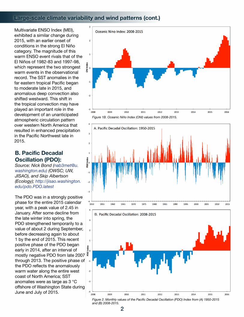
Sea surface temperature (SST) anomalies in the equatorial Pacific Ocean became more strongly positive over the course of the 2015 calendar year, culminating in a strong El Niño by fall. In specific terms, the Oceanic Niño Index (ONI), which reflects SST anomalies in the Niño3.4 region of the equatorial Pacific, increased in value from about 0.5 early in the year to greater than 2 late in the year (Figure 1), with the highest value since 1950 (2.36) recorded in November. Another commonly used indicator, the

Figure 1A. Oceanic Niño Index (ONI) values from 1950-2015.

1

Large-scale climate variability and wind patterns (cont.)

Multivariate ENSO Index (MEI), exhibited a similar change during 2015, with an earlier onset of conditions in the strong El Niño category. The magnitude of this warm ENSO event rivals that of the El Niños of 1982-83 and 1997-98, which represent the two strongest warm events in the observational record. The SST anomalies in the far eastern tropical Pacific began to moderate late in 2015, and anomalous deep convection also shifted westward. This shift in the tropical convection may have played an important role in the development of an unanticipated atmospheric circulation pattern over western North America that resulted in enhanced precipitation in the Pacific Northwest late in 2015.

B. Pacific Decadal Oscillation (PDO):Source: Nick Bond (nab3met@u.washington.edu) (OWSC; UW, JISAO), and Skip Albertson (Ecology); http://jisao.washington.edu/pdo.PDO.latest

The PDO was in a strongly positive phase for the entire 2015 calendar year, with a peak value of 2.45 in January. After some decline from the late winter into spring, the PDO strengthened temporarily to a value of about 2 during September, before decreasing again to about 1 by the end of 2015. This recent positive phase of the PDO began early in 2014, after an interval of mostly negative PDO from late 2007 through 2013. The positive phase of the PDO reflects the anomalously warm water along the entire west coast of North America; SST anomalies were as large as 3 °C offshore of Washington State during June and July of 2015.

2

Figure 2. Monthly values of the Pacific Decadal Oscillation (PDO) Index from (A) 1950-2015 and (B) 2008-2015.

Figure 1B. Oceanic Niño Index (ONI) values from 2008-2015.

Large-scale climate variability and wind patterns (cont.)

C. North Pacific Gyre Oscillation (NPGO):Source: Christopher Krembs (christopher.krembs@ecy.wa.gov), and Skip Albertson (Ecology); http://www.ecy.wa.gov/programs/eap/mar_wat/index.html

The NPGO has been mostly in the positive phase from 1998 through 2013 with the exception of 2005 to 2007 when monthly values were negative (Figure 3). Since October 2013, however, NPGO values have trended negatively, continuing into 2014 and 2015. Declining NPGO values suggest that primary productivity is decreasing along Washington’s coastline and within the California Current System.

3

Figure 3. Monthly values of the North Pacific Gyre Oscillation index (NPGO) from (A) 1950-2015 and (B) 2008-2015.

Large-scale climate variability and wind patterns (cont.)

D. Upwelling index:Upwelling favorable winds (i.e., equatorward winds) on the Washington coast bring deep ocean water in through the Strait of Juan de Fuca and into Puget Sound. The upwelled water is relatively cold and salty, with low oxygen, low pH, and high nutrient concentrations. The typical upwelling season for the Pacific Northwest is from April through September, while downwelling typically occurs during the wet winter season.

Source: Skip Albertson (skip.albertson@ecy.wa.gov), Christopher Krembs, Mya Keyzers, Laura Hermanson, Julia Bos, and Carol Maloy (Ecology); http://www.ecy.wa.gov/programs/eap/mar_wat/index.html

Monthly mean values of the upwelling index at 48 °N and 125 °W in 2015 were mostly within historic (1967-present) interquartile ranges except in May and June when coastal upwelling was significantly stronger than normal (Figure 4). In December, downwelling came close to stronger than normal conditions.

4

Figure 4. Monthly mean values of the PFEL coastal upwelling index for 2015 (red and black dots) are presented in historical statistical context based on the index values at 48 °N and 125 °W from 1967 to 2014. The box plot extent represents 5th and 95th percentiles with the interquartile range between the 25th and 75th percentiles shaded green. Values falling outside the interquartile range are colored red. Pink and blue shaded areas indicate upwelling and downwelling conditions, respectively. Data source: www.pfeg.noaa.gov/products/las/docs/upwell.nc.html.

Local climate and weather

Local climate and weather conditions can also exert a strong influence on Puget Sound marine water conditions on top of the influences of longer-term large-scale climate patterns. Variations in local air temperature best explain variations in Sound-wide water temperatures (Moore et al. 2008).

A. Regional air temperature and precipitation:Source: Karin Bumbaco (kbumbaco@uw.edu) (OWSC; UW, JISAO); www.climate.washington.edu

The 2015 calendar year was the warmest on record for the Puget Sound area, and Washington as a whole, while precipitation was near-normal. Washington is divided into 10 separate climate divisions based on similar average weather conditions within a region (http://www.ncdc.noaa.gov/monitoring-references/maps/us-climate-divisions.php). This summary uses data from the Puget Sound Lowlands division that encompasses most of the Puget Sound.

The 2015 average temperature for the division was 1.4 °C (2.5 °F) warmer than the 1981-2010 normal, and ranked as the warmest year since records began in 1895. The record warmth followed a warmer than normal 2014, which currently ties 2004 as the 3rd warmest year on record. Total annual precipitation (121.5 cm) was near-normal at 107% of average.

While reporting the annual average conditions provides one perspective on the calendar year, it is also worthwhile to consider temperature and precipitation anomalies on shorter time scales. For example, only considering 2015 annual precipitation gives no indication that drought conditions were experienced across the region. Figure 5 shows monthly temperature and precipitation anomalies for the Puget Sound relative to the 1981-2010 normals, with the large seasonal precipitation extremes illustrating how annual precipitation totals could be near-normal. Overall, the winter of 2014-2015 (October-March) had near-normal precipitation across WA State, but the extremely warm temperatures caused precipitation to fall as rain rather than snow in the mountains. Warm and dry spring conditions that

included a record warm June (Figure 5) worsened what began as a snowpack drought. The drought conditions caused record low streamflow in July, but a few heavy rain events in August helped ease some of the drought impacts. Notably, heavy rain fell in the Puget Sound region on August 14th and then again on the 29th (with high wind, too). The calendar year ended with a much wetter than normal December, ranking as the 3rd wettest December in the Puget Sound region.

Figure 5. Monthly anomalies for (A) temperature (Celsius) and (B) precipitation (centimeters) for the Puget Sound Lowlands climate division in Washington State for the 2015 calendar year. Anomalies are relative to 1981-2010 climate normals.

5

A.

B.

Local climate and weather (cont.)

Sunset over the San Juans. Photo: Breck Tyler

B. Local air temperature and solar radiation:Source: Skip Albertson (skip.albertson@ecy.wa.gov), Christopher Krembs, Mya Keyzers, Laura Hermanson, Julia Bos, and Carol Maloy (Ecology); http://www.ecy.wa.gov/programs/eap/mar_wat/index.html

Local air temperatures in 2015 were significantly warmer than normal with the exception of September and November, which were below normal. Figure 6A shows anomalies in daily air temperatures at Sea-Tac Airport, relative to a 1971-2000 historical baseline period.

Anomalies of daily solar energy flux, measured by a PAR sensor located at the University of Washington Atmospheric Sciences building (ATG), were generally above normal from May through September (Figure 6B, red shaded area). Solar energy fluxes often approached the theoretical maximum during this same period. December, however, was particularly gloomy with lower than normal sunlight for the entire month (Figure 6B, solid blue shaded area).

The waters of Puget Sound are a mix of coastal ocean water and river inputs. Monitoring the physical and biochemical processes occurring at the coastal ocean provides insight into this important driver of marine water conditions in Puget Sound.

6

Figure 6. Air temperature anomalies (A) and daily solar energy flux (B) at Sea-Tac Airport and UW, respectively, in 2015. Red shading in (A) indicates higher than average and blue indicates lower than average air temperature. The solid red line on the solar energy panel (B) shows the highest theoretical solar energy for this latitude, and the blue line is the solar energy if completely overcast. Red shading indicates when the sky is more than 50% clear (sunnier) and blue shading indicates when it is less than 50% clear (cloudier).

A.

B.

Coastal ocean and Puget Sound boundary conditions

Recovering the Chá Bă mooring aboard the R/V Thomas G. Thompson. Photo: Rachel Wold

7

A. NW Washington Coast water properties:Source: John Mickett (jmickett@apl.uw.edu) and Jan Newton (UW, APL); http://www.nanoos.org

The Northwest Association of Networked Ocean Observing Systems (NANOOS) and the University of Washington (UW) maintain two moorings, a large surface mooring called Chá Bă and an adjacent profiling mooring called NEMO-subsurface, that collect oceanographic and meteorological observations on the NW Washington shelf. At the start of the 2015 mooring deployments in late May, the anomalously warm and fresh “blob” water that was detected at the end of the 2014 deployment in October (Figure 7A, B) was no longer present and upwelling conditions were already well underway. The coldest and saltiest (and thus most dense) upwelled water was observed at depth in mid-June despite upwelling-favorable winds continuing through July and August (Figure 8A). After the coldest (~7 °C) water was observed in June, deep (85 m) water temperature slowly increased by 0.5 °C over 3.5 months until early October, then warmed more rapidly with the onset of more persistent downwelling winds and likely onshore transport of “blob” waters, reaching 10 °C at end of the deployment on Nov 19th 2015. For the period between mid-July and mid-October 2015, deep water temperature was warmer than all previous years recorded (2012-2014). Over the same period, 2015 salinity steadily decreased and was almost always fresher than past records. This may indicate a warmer and fresher source for upwelled waters.

As with other years, deep DO values in 2015 were highly variable on 1-2 week timescales, with changes coincident with changes in wind forcing and along-shelf flow (Figures 7C, 8C). The latter suggests that these changes are largely advective, meaning that horizontal gradients of DO move past the mooring site. As has been observed in previous years (2013, 2014), decreases in DO were often associated with

shifts in wind from upwelling to downwelling-favorable, with associated along-shelf flow switching from the north to the south (Figure 8A, C, E). This observation is consistent with low-DO regions forming in summer on the shelf south of the mooring site (Siedlecki et. al 2015). Lowest near-bottom values of around 1 mg/L (at 85 m) occurred in late July, in contrast to other years when deep DO continued to drop through summer, again indicating a difference in upwelling source water.

The first at-depth (50 m) record of pH at this mooring site (Figure 7D) shows that variations in pH closely follow changes in DO and appear closely linked to upwelling processes and along-shelf transport (Figure 8).

7

Figure 7. Deep (80 m) water properties at the Chá Bă mooring: (A) temperature, (B) salinity, (C) dissolved oxygen. (D) 50 m pH as measured by the SeaFET at Chá Bă compared to 50 m dissolved oxygen measured by the profiler on the nearby NEMO-subsurface mooring.

Coastal ocean and Puget Sound boundary conditions (cont.)

B. Ocean and atmospheric CO2:Source: Simone Alin (simone.r.alin@noaa.gov), Christopher Sabine, Richard Feely (NOAA, PMEL), Adrienne Sutton, Sylvia Musielewicz (UW, JISAO), Jan Newton, and John Mickett (UW, APL); http://pmel.noaa.gov/co2/story/La+Push and http://pmel.noaa.gov/co2/story/Cape+Elizabeth; PMEL contribution number 4490

Carbon dioxide (CO2) sensors have measured atmospheric and surface seawater xCO2 (mole fraction of CO2) at three-hour intervals on the surface Chá Bă mooring off La Push since 2010, mostly from spring through fall, and year-round on the National Data Buoy Center (NDBC) mooring 46041 at Cape Elizabeth since 2006, both supported by NOAA and IOOS. Because Cape Elizabeth deployments are typically year-round, we can compare these results

from winter/downwelling (October–March) and summer/upwelling (April–September) seasons with the deployments off La Push, which have mostly been during upwelling seasons.

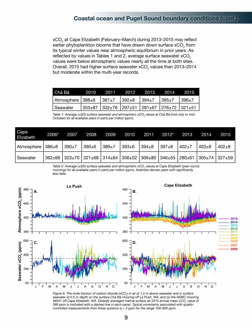
In 2015, the atmospheric xCO2 range was 387–435 ppm (parts per million) at Chá Bă (Figure 9A) and 385–436 ppm at Cape Elizabeth (Figure 9B). During all years at Cape Elizabeth, the annual average atmospheric xCO2 value ranged from 2.3–7.3 ppm higher than the globally averaged marine surface air annual mean xCO2 value reported through NOAA’s Earth System Research Laboratory web site (esrl.noaa.gov/gmd/ccgg/trends/global.html#global). In contrast, the atmospheric averages for the periods of overlap between Cape Elizabeth and Chá Bă moorings agreed within < 1 ppm in all years except 2014, which showed a 1.6 ppm difference (mid-July to mid-October data only, comparison not shown in tables). Both Chá Bă and Cape Elizabeth atmospheric time-series showed tight regressions for increasing annual average and minimum xCO2 values over the length of their respective records. At both sites, average atmospheric xCO2 has increased by 1.8–1.9 ppm yr-1 since deployment (R2 values > 0.81), which is slightly lower than the globally averaged marine surface air xCO2 rate of increase of 2.1–2.3 ppm yr-1 over the period of the moorings (full range 1.7–3.0 ppm yr-1, with annual uncertainties of 0.05-0.1 ppm yr-1). Annual minimum atmospheric xCO2 values have also increased by 1.5–2.1 ppm yr-1 at both sites, with summers at Cape Elizabeth having a higher rate of increase than winters. Maximum atmospheric xCO2 is quite variable at both sites, nonetheless it appears that the seasonal and annual maxima are increasing at Cape Elizabeth (R2 values < 0.41).

Surface seawater xCO2 ranged from 118 to 421 ppm at Chá Bă (Figure 9C) during its May–November 2015 deployment and ranged from 162 to 432 ppm at Cape Elizabeth (Figure 9D) during eight months of operation in 2015 (no data March–June). Both sites show a tendency toward lower surface seawater xCO2 through the full time-series (R2 values 0.12 to 0.36), though the patterns are weak relative to magnitude of variability and may simply reflect interannual variability. A decrease in summer variability and lower maxima were observed at both Chá Bă and Cape Elizabeth during 2013–2015 and may be related to upwelling dynamics. The early wintertime drop in

8

Figure 8. 2015 conditions at the NANOOS coastal mooring site: (A) along shore winds, with southerly winds positive (to north) and northerly winds negative (to south), (B) salinity with temperature contours over-plotted, (C) dissolved oxygen with salinity contours over-plotted, (D) nitrate concentration with salinity contours over-plotted, (E) along-shore velocity (positive to north) with salinity contours over-plotted.

Coastal ocean and Puget Sound boundary conditions (cont.)

xCO2 at Cape Elizabeth (February–March) during 2013–2015 may reflect earlier phytoplankton blooms that have drawn down surface xCO2 from its typical winter values near atmospheric equilibrium in prior years. As reflected by values in Tables 1 and 2, average surface seawater xCO2 values were below atmospheric values nearly all the time at both sites. Overall, 2015 had higher surface seawater xCO2 values than 2013–2014 but moderate within the multi-year records.

Cape Elizabeth 2006* 2007 2008 2009 2010 2011 2012* 2013 2014 2015

Atmosphere 386±8 390±7 390±6 389±7 393±6 394±8 397±8 402±7 403±8 402±8

Seawater 362±66 323±70 321±68 314±64 356±52 306±80 346±55 280±61 305±74 327±59

Chá Bă 2010 2011 2012 2013 2014 2015Atmosphere 388±6 387±7 392±8 394±7 395±7 396±7Seawater 353±87 332±76 297±51 281±67 276±72 321±51

Table 1: Average (±SD) surface seawater and atmospheric xCO2 values at Chá Bă (mid-July to mid-October) for all available years in parts per million (ppm).

Table 2: Average (±SD) surface seawater and atmospheric xCO2 values at Cape Elizabeth (year-round) moorings for all available years in parts per million (ppm). Asterisks denote years with significantly less data.

Figure 9. The mole fraction of carbon dioxide (xCO2) in air at 1.5 m above seawater and in surface seawater at 0.5 m depth on the surface Chá Bă mooring off La Push, WA, and on the NDBC mooring 46041 off Cape Elizabeth, WA. Globally averaged marine surface air 2015 annual mean xCO2 value of 399 ppm is indicated with a dashed line in each panel. Typical uncertainty associated with quality-controlled measurements from these systems is < 2 ppm for the range 100–600 ppm.

9

River inputs

The waters of Puget Sound are a mix of coastal ocean water and river inputs. The flow of rivers that discharge into Puget Sound is strongly influenced by rainfall patterns and the elevation of mountains feeding the rivers. Freshwater inflows from high elevation rivers peak twice annually from periods of high precipitation in winter and snowmelt in spring and summer. Low elevation watersheds collect most of their runoff as rain rather than mountain snowpack and freshwater flows peak only once annually in winter due to periods of high precipitation. The salinity and density-driven circulation of Puget Sound marine waters are influenced by river inflows.

A. Fraser River:Source: Ken Dzinbal (ken.dzinbal@psp.wa.gov) (PS Partnership) and Environment Canada; https://wateroffice.ec.gc.ca/index_e.html

For the 2015 calendar year, Fraser River discharges reached new peaks early in the year and new lows during summer, with a shifted hydrograph due to unusually warm climate conditions. The Fraser River is the largest single source of freshwater to the Salish Sea, accounting for roughly two-thirds of all river inflow. The normal flow regime is characterized by a single, early summer discharge peak. Fraser River waters can strongly influence conditions in the Strait of Juan de Fuca including the water entering Puget Sound through Admiralty Inlet, so the unusual 2015 flows led to altered Puget Sound water quality conditions.

The timing of the seasonal discharge impacts circulation and food web processes. In 2015, an earlier than normal discharge meant flows exceeded historic mean levels through most of the spring, with anomalously high flows in late March and April. This was followed by a severe (Level 4) drought during summer (June – September) with flows reaching historic minimums in July and August. Discharge returned to normal in October and generally remained at normal or just slightly above mean levels through the end of the year (Figure 10).

B. Puget Sound rivers:Source: Ken Dzinbal (ken.dzinbal@psp.wa.gov) (PS Partnership) and U.S. Geological Survey; http://waterdata.usgs.gov/wa/nwis/current/?type=flow

For the 2015 calendar year, Puget Sound river discharges exhibited anomalously early and extreme seasonal patterns due to unusually warm climate conditions although the overall annual discharge was near average. River flows were unusually high in the early spring as warm temperatures resulted in precipitation falling as rain when it would normally fall as snow, then dropped below median levels in early April, falling to extremely low levels through the summer drought. In most systems, flows remained abnormally low until early September (the Puyallup remained low until November), after which a series of extremely big discharge pulses were recorded, corresponding to strong rain events (Figure 11).

Puget Sound rivers contribute about one-third of freshwater inflow to the Salish Sea, with the largest volume coming from the Skagit River. In contrast to the Fraser, many Puget Sound rivers exhibit two discharge peaks per year – a peak in early summer produced by melting mountain snowpack, followed by a second peak later in the year coinciding with fall and winter rains.

10

Figure 10. Fraser River daily discharge (m3/s) at Hope, B.C. for 2015, compared to the mean value from long-term records (1912-2015). (Note 1 m3/s = 35.3 cfs).

River inputs (cont.)

Figure 11. Daily discharge (cfs) at stations in Nooksack, Skagit, Snohomish, Puyallup, Nisqually, and Skokomish Rivers in 2015, compared to long-term median values. Note the period of record varies and is indicated separately for each station.

11

Water quality

Temperature and salinity are fundamental water quality measurements. They define seawater density and are important for understanding estuarine circulation and conditions favorable to Puget Sound’s marine life. Many marine organisms have developed tolerances and life-cycle strategies for specific thermal and saline conditions. Nutrients and chlorophyll give insight into the production of organisms at the base of the food web. Phytoplankton are assessed by monitoring chlorophyll-a, their photosynthetic pigment. In Puget Sound, like most marine systems, nitrogen nutrients sometimes limit phytoplankton growth. On a mass balance, the major source of nutrients is from the ocean; however, rivers and human sources also contribute to nutrients loads. Dissolved oxygen in Puget Sound is quite variable spatially and temporally and can quickly shift in response to wind, weather patterns and upwelling. In some parts of Puget Sound, dissolved oxygen is measured intensively to understand the connectivity between hypoxia and large fish kills. Dissolved oxygen also is an indicator of biological production, respiration and consumption of organic matter, and a component for understanding the health of the food web.

A. Puget Sound long-term stations:

Ecology maintains a long-term station monitoring network throughout the southern Salish Sea including the eastern Strait of Juan de Fuca, San Juan Islands and Puget Sound basins. This network of stations provides the temporal coverage and precision needed to identify long-term trends; www.ecy.wa.gov/programs/eap/mar_wat/mwm_intr.html.

i. Temperature and salinity: Source: Julia Bos (jbos461@ecy.wa.gov), Christopher Krembs, Skip Albertson, Mya Keyzers, Laura Hermanson and Carol Maloy (Ecology)

In 2015, water temperatures were warmer than the historic record throughout all Puget Sound basins and depths for nearly the entire year. This anomaly started in the fall of 2014, when warmer than normal waters associated with the “blob” entered Puget Sound. Departures (anomalies) from historical baselines showed temperature (calculated as thermal energy content) in the 0-50 m layer of the water column to be abnormally warm (Figure 12A). The 2015 anomaly was unusually high relative to the previous decade (Figure 12D).

Warmer than normal air temperatures in early spring prematurely melted mountain snowpack, leading to higher than normal river flows. In response, salinity in Puget Sound was lower (fresher) than normal. Due to wide-spread drought conditions in summer, river flows reached new historical lows resulting in higher than normal salinities. Record rain in November and December produced abnormally high river flows causing unusually low salinities again. The large seasonal swings relating to these events is reflected in surface salinities, illustrating that the timing of freshwater supply to Puget Sound was very different in 2015 (Figure 12B). However, on an annual basis, salt content was at baseline conditions compared to the previous decade as the extremes that occurred on shorter timescales averaged out (Figure 12E).

Temperature and salinity patterns impacted the water column vertical density structure (stratification) and the energy required to thoroughly mix it (reported as delta potential energy). A more stratified water column requires more energy to completely mix. Puget Sound is typically stratified because of surface freshwater inputs, and a negative anomaly requires more tidal or wind energy to mix than normal whereas a positive anomaly means that it is more mixed than normal. With higher than normal river flows, the water column was more stratified during the first part of 2015 and less stratified when river flows declined. This is important as more mixing by tides and winds can occur with less stratification, allowing substances to mix deeper. This has implications for the food web and energy cycling, with more organic matter, surface oxygen, and nutrients reaching the seafloor when the water column

12

Water quality (cont.)

13

Figure 12. Heat maps of Puget Sound thermal energy (A) salt content (B) and potential energy (C) anomalies for the 0-50 m water layer for 2005-2015. Anomalies are calculated from site-specific monthly averages using a reference baseline established for 1999-2008. Green = lower, red = higher, black = expected, gray = no data.

A.

B.

C.

Water quality (cont.)

is less stratified. This also means that waste water, pollutants from land, and other particles will mix more deeply rather than leaving the Sound. Seasonal stratification expressed as delta potential energy closely followed the pattern of surface salinity. Note that these seasonal variations also averaged out on an annual timescale (Figure 12F).

ii. Dissolved oxygen: Source: Julia Bos (jbos461@ecy.wa.gov), Christopher Krembs, Skip Albertson, Mya Keyzers, Laura Hermanson and Carol Maloy (Ecology)

In order to put DO measurements into a Puget Sound-wide context, Ecology reports a DO “deficit”. The DO deficit is the difference between the measured value and the theoretical fully saturated value integrated over depths greater than 20 meters, not including supersaturated results. When the DO deficit is high, measured DO in the water column is low (i.e., there is a large deficit between the amount of oxygen in the water and the amount that it could hold if it was fully saturated), and when the DO deficit is low, measured DO is closer to full saturation. A Puget Sound-wide annual anomaly in the DO deficit is calculated from averaged monthly site-specific anomalies across all core monitoring stations deeper than 20 meters in Puget Sound (n = 14).

14

Figure 12. Puget Sound-wide annual anomalies for temperature (D), salinity (E), and potential energy (F) in the 0-50 m water layer from 2005-2015.

D.

E.

F.

Figure 13A. Puget Sound monthly dissolved oxygen (DO) deficit anomalies from 2005-2015 for water deeper than 20 m using a reference baseline established from 1999- 2008. (A) Puget Sound-wide annual anomaly of the DO deficit from 2005-2015.

A.

Water quality (cont.)

At the beginning of 2015, the deficit was very high and was associated with warmer ocean “blob” water that entered Puget Sound. However, lower than normal summer river flows due to drought conditions caused less stratification of the water column, allowing for increased vertical mixing, and DO recovered, especially in the Central and South Sound Basins. A heat map of monthly anomalies of the DO deficit for water deeper than 20 meters for the period 2005-2015 is shown in Figure 13B. The DO deficit was high from 2005-2008 and decreased from 2009-2012 (green), revealing improved oxygen conditions below 20 meters. In 2013, the DO deficit shifted to higher than normal values (red), especially at northern sites, continuing into 2014. The anomaly in the DO deficit shows that the 2015 DO deficit was comparable to 2013 and 2006 (Figure 13A).

iii. Nutrients and chlorophyll:Source: Christopher Krembs (christopher.krembs@ecy.wa.gov), Carol Maloy, Julia Bos, Mya Keyzers, and Laura Hermanson (Ecology) Long-term patterns and trends in Puget Sound nutrients and chlorophyll-a are determined by comparing Ecology’s monthly data to baseline conditions (1999-2008) and generating sitespecific anomalies. The average of monthly anomalies at all of Ecology’s Puget Sound monitoring stations is used to track largescale interannual changes.

Starting in 1999, monthly anomalies in the macro-nutrients nitrate and phosphate increased until around 2009 and then decreased (Figure 14A). The low nitrate levels observed in 2015 were close to conditions observed in the early 2000’s and are a result of the extreme conditions that characterized the year – the “blob”, the drought, and the rain. The “blob” was

characterized by low nutrients and these waters entered Puget Sound to influence 2015 nitrate values; the drought slowed estuarine circulation, reducing nutrient input from the ocean in the summer and increasing residence times which allowed organisms to better exploit nutrient pools; and strong rain events in the fall and winter diluted nutrients in Puget Sound. Annual averages of chlorophyll-a anomalies declined from 1999 until around 2013 (Figure 14B, C). The importance of biological uptake of nutrients is reflected in the robust but negative correlation of nitrate and chlorophyll-a (Figure 14C). The negative correlation prevailed in 2015, a year of high anomalies in temperature and salinity.

The silicate-to-nitrogen ratio (Si:DIN), a potential indicator of human nitrogen inputs (Figure 14B) declined by 10 units per decade until 2013 (Spearman Rank Correlation rh = -0.62, p < 0.05, n = 15), primarily driven by changes in nitrate. This trend appears to be in step with the trend in chlorophyll-a.

The mean seasonal cycle (1999-2015) of chlorophyll-a and ammonium shows that the spring bloom typically occurs in May, followed by elevated ammonium in June (Figure 14D). A broad summer bloom generally occurs in August, followed by increases in ammonium in September. The year 2015 was different in that the spring bloom occurred one month early in April and ammonium concentrations in June were much higher than previous years. The fall peak in ammonium was also shifted one month later in the season. During the last 16 years, the summer chlorophyll-a maxima seem to have fallen (Figure 14E). In 2015, the late summer bloom was comparable to the long-term baseline (Figure 14D).

15

B.

Figure 13B. Puget Sound-wide annual anomaly of the DO deficit from 2005-2015. (B) Heat map of monthly anomalies calculated from site-specific monthly averages. Green = lower, red = higher, black = expected, gray = no data.

Water quality (cont.)

Despite the low ambient nutrient concentrations, macro-algae abundance was very high in 2015 (Figure 14F). This again is indicative of primary producers converting ambient nutrients into organic biomass.

16

Figure 14. Puget Sound-wide annual anomalies of (A) nitrate (black circles) and phosphate (open diamond), (B) the ratio of Si:DIN (open circles) and chlorophyll-a (black diamonds) over the period of 1999-2015. (C) Puget Sound-wide long-term anomalies of nitrate plotted against chlorophyll-a. (D) Puget Sound-wide monthly averages of chlorophyll-a (green circles) and ammonium (red circles) for 2015, and the mean seasonal cycle based on 1999-2013 values (faint green line, chlorophyll-a; faint red line, ammonium). (E) Long-term trends in Puget Sound-wide average phytoplankton biomass, with annual averages (triangles) and maxima specific to the July - December period (circles), highlighting a distinctive decline in late summer. (F) Example of macroalgae occurring in Central Sound in July 2015.

Water quality (cont.)

iv. Water mass characterization:Source: Skip Albertson (skip.albertson@ecy.wa.gov), Christopher Krembs, Mya Keyzers, Laura Hermanson, Julia Bos, and Carol Maloy (Ecology);http://www.ecy.wa.gov/programs/eap/pscoastalintro.htm

Water preferentially travels and mixes along similar densities. Using monthly data from Ecology’s long-term marine monitoring program, we identify warm water masses (> 15 °C) in Puget Sound’s Central, Whidbey, Hood Canal, and South basins (Figure 15A). Warmer temperatures are associated with lower densities (sigma-t = 18-22), shallow depths (2-4 m, and to 9 m in South basin), and are observed mainly in the summer months. The warm water masses of similar temperatures became denser during summer, driven by increasing salinity (implied in the data). Especially warm water (> 19 °C) occurred in Hood Canal and South Puget Sound in July and August. Also notable was the length of time (5 months) that > 15 °C water persisted in these regions.

A simple estimate of residence time, based on a Knudsen relationship using river flow and Ecology core station salinity records, was calculated for the upper 30 meters of the Central Basin during the summer months (May through August; Figure 15B). In 2015, the drought caused surface and bottom salinities to be similar, increasing the residence time. This is important because residence time has a significant impact on the concentration of pollutants that can build up in the

system. Residence time is displayed here as an index relative to a 16-year baseline. Residence time of water in Puget Sound was higher in 2015 compared to the past nine years (2007-2014) but less than in 2002, 2003, and 2006; years that also had periods with warm, dry conditions.

17

Figure 15. (A) Monthly plots of water temperatures exceeding 15 °C versus density with color showing temperature exceedance. Results are shown for Central, Whidbey, Hood Canal, and South basins. (B) Residence time index for Central Basin.

A.

B.

Water quality (cont.)

B. Puget Sound profiling buoys:

Profiling buoys take frequent (> daily), full-depth measurements of water properties that allow characterization of both short-term and long-term processes, including deep water renewal events and tracking water mass properties. There are currently six ORCA (Oceanic Remote Chemical Analyzer) moorings in Puget Sound, maintained by UW and NANOOS, with data from four moorings presented here: southern Hood Canal (Twanoh and Hoodsport), Dabob Bay, and southern Puget Sound (Carr Inlet).

i. Temperature:Source: Wendi Ruef (wruef@uw.edu), Al Devol (UW), John Mickett and Jan Newton (UW, APL); http://orca.ocean.washington.edu, http://www.nanoos.org

Observations from the UW ORCA mooring program show that Puget Sound waters experienced unprecedented, full-depth warm water anomalies throughout 2015 (Figure 16A, B). Most locations were in excess of 2 °C above the 10-year observational means (2005-2014), and highs of up to 7 °C above the observational means were seen in the surface waters in southern Hood Canal in June (off scale in Figure 16A). The temperature anomalies observed in Puget Sound and Hood Canal during 2015 were

a direct contrast to the predominantly colder than average temperatures observed during 2014. While Carr Inlet alone showed warm temperature anomalies during 2014, these were more intense during 2015. While in general the entire water column at Twanoh in 2015 was anomalously warmer, there were short-lived pulses of colder than average waters at the surface during summer and early fall (Figure 16A), likely due to wind-driven seiche-like motions (i.e., standing wave) in the basin lifting cooler deep waters towards the surface.

In early winter 2015, temperatures in Puget Sound deep waters remained constant through early to mid-summer, without the typical cooling observed in previous years (Figure 16C-E), and with temperatures reaching 2 full standard deviations above climatological averages by the beginning of May. This lack of cooling, coupled with fresher than normal waters in early winter months due to the “blob” (see Salinity section), contributed to the least dense waters observed in Hood Canal in the 10-year time series. The comparatively more dense oceanic waters entering during 2015 effectively displaced the resident waters, with the flushing in Hood Canal complete by the end of August 2015, nearly 6 weeks earlier than observed in the data record, bringing even further extreme temperature anomalies to southern Hood Canal (> 2.5 °C above climatologies, Figure 16D-E).

18

Figure 16. (A) and (B): 2015 water temperature anomalies (compared to 2005-2014 average) for Twanoh and Carr Inlet. Data are colored by a white threshold at 0, with red indicating warmer and blue colder than historical average conditions. (C), (D), (E): 2015 data (cyan line), climatology (dark blue line), and all historical data (grey lines) for near bottom water temperature at Carr Inlet, Hoodsport, and Twanoh; also shown are ± 1 and 2 SDs from the climatology.

Water quality (cont.)

ii. Salinity:Source: Wendi Ruef (wruef@uw.edu), Al Devol (UW), John Mickett and Jan Newton (UW, APL); http://orca.ocean.washington.edu, http://www.nanoos.org

Observations from the UW ORCA mooring program show that salinity during 2015 varied in three distinct periods: 1) in early 2015 the lingering influence of the “blob”, which entered Puget Sound in late 2014, contributed to full-water column salinities that were fresher than long-term averages; 2) throughout summer more saline conditions developed as drought conditions persisted until early fall; 3) toward the end of 2015, rainfall associated with the wettest winter on record contributed to a fresher than average water column. These seasonal patterns were basin-wide and to show local variations, Twanoh in southern Hood Canal (Figure 17A) and Carr Inlet in South Puget Sound (Figure 17B) are compared. Positive salinity anomalies were observed near the surface at Twanoh earlier in the year than at Carr Inlet (Figure 17C-D), which is likely due to drought conditions affecting riverine influences in southern Hood Canal from the Skokomish River. However, because the water

column at Carr Inlet is well mixed in comparison to the stratified conditions at the Twanoh mooring, saltier than average waters extended completely through the water column at Carr Inlet approximately a month before this occurred at Twanoh. Similarly, the overall transition from fresher to saltier conditions occurred earlier in South Sound than southern Hood Canal. Both basins experienced freshening of the water column by late fall due to rain forcing, with negative salinity anomalies observed at Twanoh by mid-November.

The succession of “blob”/drought/rain influences produced an extreme salinity anomaly reversal (Figure 17E-G), as seen in the deep waters of South Sound and Hood Canal. Waters were fresher than 2 standard deviations from climatology January to March, then steadily increased in salinity through the summer to highs of 2 standard deviations above the climatology by late summer/early fall. At Carr Inlet, these extremes in spring and fall were significantly outside of 2 standard deviations of the climatology, and were respectively the highest and lowest values observed in the data record.

Figure 17. (A) and (B): Salinity data for Twanoh and Carr Inlet for 2015. (C) and (D): Salinity anomalies (2015 – climatology) for Twanoh and Carr Inlet. Data are colored by a white threshold at 0, with red indicating saltier and blue fresher than historical average conditions. (E), (F), (G): 2015 data (cyan line), climatology (dark blue line), and all historical data (grey lines) for near bottom salinity at Carr Inlet, Hoodsport, and Twanoh; also shown are ± 1 SD from the climatology (pink dotted line) and ± 2 SD from the climatology (red dotted line).

19

Water quality (cont.)

Hoodsport buoy in southern Hood Canal. Photo: Rachel Wold

iii. Dissolved oxygen:Source: Wendi Ruef (wruef@uw.edu), Al Devol (UW), John Mickett and Jan Newton (UW, APL); http://orca.ocean.washington.edu, http://www.nanoos.org

DO conditions during 2015 ranged from moderate to record lows at all moorings, and while seasonal variation was similar to previous years, conditions were shifted in timing and more intense than previously observed. The DO time-series at Twanoh in southern Hood Canal for 5 of the previous 6 years, including 2015, is shown in Figure 18. As with previous years, due to increased respiration and decreased oxygen supply, oxygen concentrations at depth gradually decreased through the spring and early summer in 2015. However, unlike in previous years, the 2015 near-bottom waters at Twanoh were intensely hypoxic (< 1 mg L-1) by June, a full 2-3 months earlier than the hypoxic layer formation in previously observed years. The 2015 hypoxic layer had some of the lowest oxygen concentrations

observed in the 10-year record. As a consequence of this intensely hypoxic water, a fish kill event occurred in southern Hood Canal on 29 August, 2015 (see call out box). The DO time-series in 2015 appears most similar to 2010, including the presence of a low oxygen layer at depth in the beginning of the year (leftover low DO-waters from incomplete flushing the previous fall), the intensity of the hypoxic layer that formed during the summer, and the occurrence of a fish kill event (Figure 18). However, the timing of these events is shifted significantly earlier in 2015, and absolute DO concentrations are lower at depth in 2015 than those observed in 2010. The annual oceanic intrusion was strong and early in 2015 (see Temperature section), with relatively higher oxygen concentrations (~3.5 mg L-1). These waters reached Hoodsport at depth in the beginning of August (see call out box), and Twanoh in September. Oxygen concentrations of near-bottom waters at Twanoh hovered around 2 mg L-1 through the end of 2015.

20

Figure 18. Time-series of DO at the Twanoh ORCA mooring from 2010 to 2015.

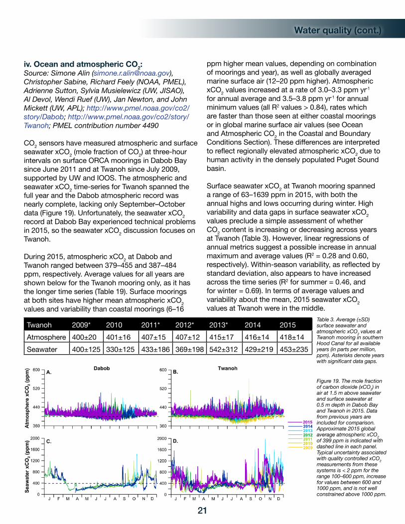
Water quality (cont.)

iv. Ocean and atmospheric CO2:Source: Simone Alin (simone.r.alin@noaa.gov), Christopher Sabine, Richard Feely (NOAA, PMEL), Adrienne Sutton, Sylvia Musielewicz (UW, JISAO), Al Devol, Wendi Ruef (UW), Jan Newton, and John Mickett (UW, APL); http://www.pmel.noaa.gov/co2/story/Dabob; http://www.pmel.noaa.gov/co2/story/Twanoh; PMEL contribution number 4490

CO2 sensors have measured atmospheric and surface seawater xCO2 (mole fraction of CO2) at three-hour intervals on surface ORCA moorings in Dabob Bay since June 2011 and at Twanoh since July 2009, supported by UW and IOOS. The atmospheric and seawater xCO2 time-series for Twanoh spanned the full year and the Dabob atmospheric record was nearly complete, lacking only September–October data (Figure 19). Unfortunately, the seawater xCO2 record at Dabob Bay experienced technical problems in 2015, so the seawater xCO2 discussion focuses on Twanoh.

During 2015, atmospheric xCO2 at Dabob and Twanoh ranged between 379–455 and 387–484 ppm, respectively. Average values for all years are shown below for the Twanoh mooring only, as it has the longer time series (Table 19). Surface moorings at both sites have higher mean atmospheric xCO2 values and variability than coastal moorings (6–16

ppm higher mean values, depending on combination of moorings and year), as well as globally averaged marine surface air (12–20 ppm higher). Atmospheric xCO2 values increased at a rate of 3.0–3.3 ppm yr-1 for annual average and 3.5–3.8 ppm yr-1 for annual minimum values (all R2 values > 0.84), rates which are faster than those seen at either coastal moorings or in global marine surface air values (see Ocean and Atmospheric CO2 in the Coastal and Boundary Conditions Section). These differences are interpreted to reflect regionally elevated atmospheric xCO2 due to human activity in the densely populated Puget Sound basin.

Surface seawater xCO2 at Twanoh mooring spanned a range of 63–1639 ppm in 2015, with both the annual highs and lows occurring during winter. High variability and data gaps in surface seawater xCO2 values preclude a simple assessment of whether CO2 content is increasing or decreasing across years at Twanoh (Table 3). However, linear regressions of annual metrics suggest a possible increase in annual maximum and average values (R2 = 0.28 and 0.60, respectively). Within-season variability, as reflected by standard deviation, also appears to have increased across the time series (R2 for summer = 0.46, and for winter = 0.69). In terms of average values and variability about the mean, 2015 seawater xCO2 values at Twanoh were in the middle.

21

Twanoh 2009* 2010 2011* 2012* 2013* 2014 2015Atmosphere 400±20 401±16 407±15 407±12 415±17 416±14 418±14Seawater 400±125 330±125 433±186 369±198 542±312 429±219 453±235

Table 3. Average (±SD) surface seawater and atmospheric xCO2 values at Twanoh mooring in southern Hood Canal for all available years (in parts per million, ppm). Asterisks denote years with significant data gaps.

Figure 19. The mole fraction of carbon dioxide (xCO2) in air at 1.5 m above seawater and surface seawater at 0.5 m depth in Dabob Bay and Twanoh in 2015. Data from previous years are included for comparison. Approximate 2015 global average atmospheric xCO2 of 399 ppm is indicated with dashed line in each panel. Typical uncertainty associated with quality controlled xCO2 measurements from these systems is < 2 ppm for the range 100–600 ppm, increase for values between 600 and 1000 ppm, and is not well constrained above 1000 ppm.

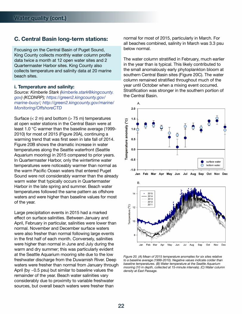
Water quality (cont.)

C. Central Basin long-term stations:

Focusing on the Central Basin of Puget Sound, King County collects monthly water column profile data twice a month at 12 open water sites and 2 Quartermaster Harbor sites. King County also collects temperature and salinity data at 20 marine beach sites.

i. Temperature and salinity: Source: Kimberle Stark (kimberle.stark@kingcounty.gov) (KCDNRP); https://green2.kingcounty.gov/marine-buoy/; http://green2.kingcounty.gov/marine/Monitoring/OffshoreCTD

Surface (< 2 m) and bottom (> 75 m) temperatures at open water stations in the Central Basin were at least 1.0 °C warmer than the baseline average (1999-2010) for most of 2015 (Figure 20A), continuing a warming trend that was first seen in late fall of 2014. Figure 20B shows the dramatic increase in water temperatures along the Seattle waterfront (Seattle Aquarium mooring) in 2015 compared to prior years. In Quartermaster Harbor, only the wintertime water temperatures were noticeably warmer than normal as the warm Pacific Ocean waters that entered Puget Sound were not considerably warmer than the already warm water that typically occurs in Quartermaster Harbor in the late spring and summer. Beach water temperatures followed the same pattern as offshore waters and were higher than baseline values for most of the year.

Large precipitation events in 2015 had a marked effect on surface salinities. Between January and April, February in particular, salinities were lower than normal. November and December surface waters were also fresher than normal following large events in the first half of each month. Conversely, salinities were higher than normal in June and July during the warm and dry summer; this was particularly evident at the Seattle Aquarium mooring site due to the low freshwater discharge from the Duwamish River. Deep waters were fresher than normal from January through April (by ~0.5 psu) but similar to baseline values the remainder of the year. Beach water salinities vary considerably due to proximity to variable freshwater sources, but overall beach waters were fresher than

normal for most of 2015, particularly in March. For all beaches combined, salinity in March was 3.3 psu below normal.

The water column stratified in February, much earlier in the year than is typical. This likely contributed to the small anomalously early phytoplankton bloom at southern Central Basin sites (Figure 20C). The water column remained stratified throughout much of the year until October when a mixing event occurred. Stratification was stronger in the southern portion of the Central Basin.

22

Figure 20. (A) Mean of 2015 temperature anomalies for six sites relative to a baseline average (1999-2010). Negative values indicate colder than baseline temperatures. (B) Water temperature at the Seattle Aquarium mooring (10 m depth, collected at 15-minute intervals). (C) Water column density at East Passage.

Water quality (cont.)

At most sites, an increase in DO levels was evident in surface waters between April and May due to the occurrence of spring phytoplankton blooms (Figure 22A). Overall, DO in surface waters was lower than the long-term baseline average (1999-2010) at most open water sites between January and early April, but rose to higher than normal levels in August and September during the late summer phytoplankton blooms. DO levels in bottom waters were also slightly below normal (~0.5-1.0 mg L-1) in January and April, followed by near normal or slightly above normal levels for the rest of the year (Figure 21B).

ii. Dissolved oxygen: Source: Kimberle Stark (Kimberle.stark@kingcounty.gov) and Stephanie Jaeger (KCDNRP); https://green2.kingcounty.gov/marine-buoy/; http://green2.kingcounty.gov/marine/Monitoring/OffshoreCTD

Twice monthly sampling at 12 sites in the Central Basin and 3 in situ moorings (15-minute intervals) indicate that DO levels in 2015 were above 5.0 mg L-1

throughout the year at all locations and depths, with the exception of East Passage and Quartermaster Harbor. DO in bottom waters at East Passage fell to 4.5 mg L-1 in early June, an unusual occurrence during this month and likely a response to the decay of a large, sustained phytoplankton bloom that occurred from late April through June. In inner Quartermaster Harbor, a site with historically low DO, levels were lowest (< 1.1 mg L-1) in late June and August and highest (> 20.6 mg L-1) in March. The high DO levels were likely due to an intense phytoplankton bloom (Figure 21A). DO levels in outer Quartermaster Harbor were lower than in open Central Basin waters, with levels < 3.0 mg L-1 recorded in late August; however, values were not as low as those observed in the inner harbor. Overall, 2015 Quartermaster Harbor DO levels were higher than in previous years and never fell below 1.0 mg L-1. Both Quartermaster Harbor moorings indicate substantial diurnal variation, particularly during bloom events.

23

Figure 21. (A) 2015 DO concentrations in inner Quartermaster Harbor (Yacht Club). Data were recorded at 1-m depth every 15-minutes. (B) 2015 DO anomalies in bottom waters at representative sites in the Central Basin. 2015 values are compared to the 1999-2010 baseline.

A.

B.

Water quality (cont.)

iii. Nutrients and chlorophyll: Source: Kimberle Stark (Kimberle.Stark@kingcounty.gov) and Gabriela Hannach (KCEL); http://green2.kingcounty.gov/marine/

Twice monthly (monthly in January and December) sampling at 14 sites and 3 in situ moorings (15-minute intervals) located in the Central Basin show that overall, 2015 chlorophyll-a levels were close to baseline levels (1999-2010, Figure 22A) and slighter lower than the high levels observed in 2014. Chlorophyll-a levels generally reflect seasonal phytoplankton bloom dynamics. Of note is a small, yet highly unusual phytoplankton bloom observed in late February 2015 in the southern portion of the Central Basin. Atypical stratification of the water column in February likely contributed to this unusual bloom (Figure 20C). Basin-wide, the spring phytoplankton bloom occurred during the third week in April, which is a couple of weeks later than the previous few years. The April bloom was dominated by the chain forming diatoms Chaetoceros spp. and Lauderia sp./Detonula sp., giving way to a May bloom dominated by the chain forming diatoms Chaetoceros spp. and Thalassiosira spp. A large bloom consisting primarily of Chaetoceros spp. occurred in late September throughout the southern portion of the Central Basin, including Quartermaster Harbor.

Nutrient levels varied seasonally and generally correlated well with chlorophyll-a and the timing of phytoplankton blooms. Seasonal decreases in surface (< 2 m) nitrate/nitrite levels were consistent with phytoplankton uptake; this decrease was particularly noticeable during the February and late fall blooms (Figure 22B). Quartermaster Harbor was the only location where nitrate/nitrite was depleted below detectable levels at various times, coinciding with large blooms. Ammonia levels in both surface and bottom waters steadily increased after the spring bloom until late June and then steadily decreased throughout the rest of the year, with the exception of October. Ammonia levels were elevated in October in the southern Central Basin following the large September phytoplankton bloom. Deep waters (> 75 m) had higher levels of ammonia and nitrate/nitrite from April through August and April through September, respectively (Figure 22C); however, surface levels were similar to baseline levels (1999-2010). Silica levels were influenced by freshwater

input, with high levels observed throughout the water column in January, early February, and December following heavy rainfall. Silica values in surface waters were low in May and early June and then again in late September as a result of uptake by diatoms during blooms.

24

Figure 22. 2015 surface water (A) chlorophyll-a and (B) nitrate levels, and (C) deep water ammonia levels at 12 sites in the Central Basin compared to the long-term baseline. The line within the box denotes the median, box boundaries are 25th and 75th percentiles, whiskers are 10th and 90th percentiles, and points are 5th and 95th percentiles.

Water quality (cont.)

Nutrient values at 20 beach sites in the Central Basin were highly variable, dependent upon location. At most sites, nitrate/nitrite was below normal for the entire/most of the year; however, at sites affected by freshwater inputs, levels were higher than normal in some months, particularly March. Total nitrogen levels were also elevated at these locations in March.

D. Ferry observations:

i. Victoria Clipper observations and Noctiluca blooms:Source: Suzan Pool (suzan.pool@ecy.wa.gov), Christopher Krembs, Julia Bos (Ecology), and Brandon Sackmann (Integral Consulting, Inc.); http://www.ecy.wa.gov/programs/eap/mar_wat/index.html

Noctiluca scintillans is a heterotrophic dinoflagellate that appears in high abundances in eutrophied coastal environments (Vasas et al. 2007). In Puget Sound, it may be an indicator for changes in water quality that impact lower trophic food webs. The seasonal patterns of ammonium and chlorophyll in relation to Noctiluca blooms suggest an important role of Noctiluca in material cycling within Central Sound in early summer.

Ferry-based monitoring from the Victoria Clipper IV began in 2010 as a time-efficient and cost-effective means of measuring a large and representative area of Puget Sound surface waters. Data from regular ferry routes were analyzed with data from monthly water column stations and aerial photographs to document Noctiluca blooms. During ferry transits between

Seattle and Victoria, B.C., an optical fluorometer measures temperature and chlorophyll fluorescence at 5-sec intervals. Data are georeferenced and focus on the area between Admiralty Sill (~48 °N) and Seattle (~47.6 °N). Optical chlorophyll measurements are compared with monthly samples collected for chlorophyll-a and ammonium from nearby monitoring stations at discrete depths (0, 10 and 30 m). Median chlorophyll-a and ammonium concentrations are compared to baseline levels from 1999 to 2013.

In 2015, Noctiluca blooms coincided with high levels of ammonium and low chlorophyll-a concentrations in the water column (Figure 23A). Noctiluca blooms occur in a temperature range between 10 and 13 °C, yet the mass accumulation at the surface was independent of temperature (Figure 23B). Chlorophyll fluorescence was high during periods when no accumulations of Noctiluca were visible from aerial overflights.

Seasonal ammonium peaks coincided with suppressed chlorophyll-a concentrations and two Noctiluca blooms (Figure 23A,B). Subjectively, Noctiluca blooms appeared weaker in 2015 than in 2011 (Figure 23B), the first summer with available data from ferry transect surface monitoring.

Warm water can favor some HAB forming species. In 2015, areas with warm water (temperatures > 15 °C) were more extensive and prolonged compared to 2011 and 2012 (Figure 23B), potentially widening the seasonal window for HABs.

25

A.

Figure 23A. Median and baseline data (1999 to 2013) from discrete samples at five monthly monitoring stations from all sampling depths (0, 10, and 30 m).

Water quality (cont.)

Suzan Pool and Brandon Sackmann aboard the Victoria Clipper IV. Photo: Christopher Krembs

26

Figure 23B. Spatial and temporal connectivity between Noctiluca and phytoplankton concentrations in Puget Sound in June of 2011, 2012 and 2015. Shown are aerial photographs of Noctiluca blooms (Panel a) and contour plots from daily ferry transits from April through September (Panel b), and maps of daily ferry transits on days with Noctiluca blooms (Panel c). Red boxes in Panel b show the response of phytoplankton in surface water to Noctiluca, as periods of reduced chlorophyll concentrations are coincident with large Noctiluca blooms rising to the surface and visible from higher altitudes. Panel c shows the geographical extent and location of the impact of Noctiluca on surface phytoplankton concentrations in Central Sound on selected days of June. Photo: Christopher Krembs

B.

Water quality (cont.)

E. North Sound surveys:

i. Padilla Bay temperature:Source: Jude Apple (japple@padillabay.gov), Nicole Burnett, and Heath Bohlman (Padilla Bay NERR); www.padillabay.gov

Padilla Bay is a tidally-influenced shallow (< 5m) embayment north of Puget Sound and part of the National Estuarine Research Reserve System (NERRS). The Reserve maintains four long-term (> 20yrs) monitoring stations throughout the bay which provide high frequency (15-min interval) measurements of water quality parameters. Monitoring data reveal that water temperature is highly variable in Padilla Bay, with an annual range from 3 to 24 °C and daily fluctuations approaching 10 °C in summer months. Despite this large interannual variability, mean water temperature in 2015 (11.7±0.01 °C) was significantly higher (p < 0.001) than all other years since continuous monitoring began in 1995. Prior to 2015, 1997 and 1998 had the highest mean temperatures on record in Padilla Bay (11.1 °C). Warmer water temperatures in 2015 are evident in a comparison of daily water temperatures to the long-term (1995-2014) daily mean (Figure 24A). Particularly noticeable in 2015 were sustained periods of higher temperatures (> 1 °C) in winter (January-February) and early fall (September-October), as well as anomalously high excursions in summer (June and August). The warm conditions observed in Padilla Bay in 2015 are unprecedented in our long-term dataset, as evidenced by annual temperature anomalies which highlight these exceptionally high temperatures in 2015 (Figure 24B). Anomalously warm “blob” waters that entered Puget Sound in the fall of 2014 and unusually warm air temperatures in late spring and summer 2015 most likely contributed to these elevated temperatures in Padilla Bay. Warmer and cooler periods revealed by annual anomalies are associated with large-scale climatic cycles, as evidenced by a strong correlation with indices for the Pacific Decadal Oscillation (PDO) and El Niño Southern Oscillation (data not shown).

27

Figure 24. Long-term patterns in temperature in Padilla Bay, including (A) comparison of daily mean temperatures in 2015 with long-term (1995-2014) daily means, and (B) long-term annual temperature anomalies.

A.

B.

Water quality (cont.)

F. Snapshot surveys:Snapshot surveys take place over a short period of time and can provide intensive observations in select regions of interest. When interpreted in the context of more frequent long-term observations, snapshot surveys can reveal processes and variations in water conditions that would not otherwise be detected.

i. San Juan Channel/Juan de Fuca fall surveys:Source: Jan Newton (newton@apl.uw.edu) (APL, UW), Breck Tyler (UCSC), Krista Nunnally, Julianne Dirks, and Lily Armstrong-Davies (UW); http://courses.washington.edu/pelecofn/index.html

The University of Washington Friday Harbor Laboratories Research Apprenticeship Program has maintained a time-series of pelagic ecosystem variables during fall quarter (September – November) since 2004. Research apprentices sample two sites approximately weekly. The San Juan Channel (North) site is well-mixed with seasonal influence from the Fraser River plume, and the Strait of Juan de Fuca (South) site has classic two-layer stratification between out-flowing estuarine water and in-flowing oceanic water.

The 12-year record shows 2015 to be well above average temperature, but not as warm as 2014, based on the observations of temperature versus salinity from the sea surface to ~80 m at the South station measured during the first week of November 2004-2015 (Figure 25A). While the November 2014 temperature was more than a full degree Celsius above the previous warmest waters, the 2015 data are intermediate between that and the two prior warmest years, 2004 and 2006, which were El Niño years. The two coldest years, 2007 and 2011, were La Niña years. The 2015 data are consistent with continued influence of the “blob” and also El Niño forcing. The salinity range was more typical in November 2015, unlike 2014 when the “blob” signature was uncharacteristically fresher, indicating its surface water origin.

The effect of the widespread warm waters on regional biological organisms is still under study, but for the top predators the 2015 pattern was very similar to the preceding year (Figure 25B). The predominant marine mammal species (Harbor Porpoise, Steller Sea Lion, and Harbor Seal) exhibited very low abundance during 2014-2015; in both years, however, there has been significantly higher than normal mammal diversity,

including transient Killer Whales, Humpback Whales, and Pacific White-sided Dolphins (2014 only). Seabird abundance has remained relatively low during the period 2013-2015 but community composition during this period has not differed from longer term trends.

28

A.

B.

C.

Figure 25. (A) Temperature versus salinity from 80 m to the surface at the South station in the eastern Strait of Juan de Fuca during the first week of November. Deep waters (coldest and saltiest) are found on the right. Color coding shows: yellow=El Niño years; blue=La Niña years; gray=neutral years. (B) Marine mammal density from 2007 to 2015. (C) Marine bird density from 2009 to 2015.

CALL-OUT BOX: Fish kill in Hood Canal

Overall, the sequence of events leading to the 29 August 2015 fish kill were similar to those observed in previous fish kill events (2006, 2010): an intensely hypoxic (< 1 mg L-1) layer developed at depth throughout the summer that, with the onset of the deep inflow of the annually-occurring warm and salty oceanic intrusion, gradually shoaled upwards in the water column where it was subsequently upwelled to the surface during a strong southerly wind event. However, during 2015, the DO conditions in southern Hood Canal, and the resultant fish kill, were also significantly influenced by the anomalous characteristics of the 2014 and 2015 oceanic flushing events in terms of both intensity and timing.

The weak oceanic intrusion into Hood Canal during 2014 resulted in incomplete flushing of southern Hood Canal which failed to adequately replenish DO in the deep and near-bottom waters. Consequently, DO concentrations remained very low through winter and spring, and by late summer had reached the lowest concentrations recorded in the 10-year time series (basically anoxic, Figure 26), setting up conditions for a significant fish kill during the fall intrusion. In spring 2015, the anomalously warm and fresh “blob”-influenced waters present in

northern Hood Canal, which are source waters for lower Hood Canal, were some of the lowest oxygen concentrations observed at the Hansville mooring (Figure 26), further contributing to the developing hypoxic conditions in Hood Canal. These waters also were characterized by some of the lowest densities observed at the moorings, which were easily displaced by the incoming oceanic waters (see Temperature section 5.B.i). Thus, the oceanic intrusion reached southern Hood Canal nearly 6 weeks earlier than any previous year, and changes in the water column occurred rapidly. DO concentrations in the deep waters went from 2 standard deviations below to 2 standard deviations above the climatology in less than a month. The hypoxic layer at Hoodsport was ~100 meters thick on 31 July, but was displaced by incoming higher oxygen waters and shoaled upwards to a layer only ~20 meters thick by the end of August. When strong persistent winds from the south occurred on 28 August and upwelled the hypoxic layer to the surface, a fish kill occurred on 29 August (Figure 27). With the severity of conditions present before the wind event, a potentially large fish kill was expected. On 29 August, Skokomish Tribe Department of Natural Resources staff reported hundreds of dead crab, eelpouts (a deep water species), numerous ratfish, sculpin, gunnels, English

29

Figure 26. (A), (B), (C): 2015 data (cyan line), 2014 data (black line), climatology (dark blue line), and all historical data (grey lines) for near bottom oxygen concentrations at Hansville, Hoodsport, and Twanoh; also shown are +/- 1 SD from the climatology (pink dotted line) and +/- 2 SD from the climatology (red dotted line).

sole, and squid. They also observed wolf eels and Octopus outside of their dens during the day, and many species of deep water fish at shallow depths, including super schools of rockfish and large spot prawns and shrimp. While significant, the observed distress and mortalities were less than anticipated. The early flushing started the shoaling process earlier than normal, stopping the growth and spread of the deep hypoxic layer, and lessening the risk of additional fish kills as the season progressed. Previous fish kills occurred during September.

Author: Wendi Ruef (wruef@uw.edu), Al Devol (UW), John Mickett and Jan Newton (UW, APL); http://orca.ocean.washington.edu, http://www.nanoos.org

CALL-OUT BOX: Fish kill in Hood Canal (cont.)

30

Figure 27. Time series of surface winds at Carr Inlet (top) and dissolved oxygen concentration at Hoodsport ORCA mooring (bottom), with a subset of profiles plotted at Hoodsport. DO levels above 2 mg L-1 in the near-surface layer are not shaded for clarity.

Photo credit: Seth Book, Skokomish DNR

Plankton

Marine phytoplankton are microscopic algae that form the base of the marine food web. They are also very sensitive indicators of ecosystem health and change. Because they respond rapidly to a range of chemical and physical conditions, phytoplankton community composition can be used as an indicator of deteriorating or changing ocean conditions that can affect entire ecosystems.

A. Marine phytoplankton:Source: Gabriela Hannach (gabriela.hannach@kingcounty.gov), and Lyndsey Swanson (KCEL); http://green2.kingcounty.gov/marine/Monitoring/Phytoplankton

King County has analyzed phytoplankton samples semi-monthly in the Puget Sound Central Basin since 2008 using non-quantitative microscopy. Since May of 2014, phytoplankton has also been analyzed via FlowCAM, an imaging particle analyzer, to assess 5-300 µm particle abundance and biovolume (a biomass proxy) at 8 long term monitoring stations.

The unprecedented high water temperatures recorded in Puget Sound since the fall of 2014 and throughout 2015, coupled with a dry summer and wet fall, likely influenced the seasonal timing and magnitude of blooms. Compared to the previous year, 2015 spring and summer blooms were less marked but persisted longer, and fall blooms were limited to central and south stations only (Figure 28A). A highly unusual February bloom of the large diatom Coscinodiscus was most conspicuous at the central and south stations, largest off Duwamish Head, East Passage and Dockton (Quartermaster Harbor), and was likely enabled by an atypical occurrence of winter water column stratification. Similarly, the early fall Chaetoceros-dominated bloom showed a clear North-South gradient, and was exceptionally large at Dockton.

As in previous years, chain-forming diatoms were typically the dominant taxa from early spring to early fall (Figure 28B). Of the nine most abundant diatom genera identified, the chain-forming Thalassiosira, Lauderia/Detonula and Chaetoceros (multiple species) initiated the relatively late April spring bloom, followed by more diverse mixed diatom assemblages that

31

B.

A.

C.

Figure 28. (A) Total biovolume (gray area) and biovolume of main groups in 2015. (B) Percent contribution of five most abundant taxonomic categories per sampling event identified using FlowCAM. Plotted values in (A) and (B) are means for six main-stem sites in the Central Basin (only Point Wells in early March). Numerals above bars indicate total number of taxonomic categories out of a total of 51 categories identified by FlowCAM in 2015. Note that “Particle abundance” may refer to whole chains, fragments, or individual cells, and is not indicative of biovolume. (C) Non-metric multidimensional scaling (nMDS) ordination of all May-December 2014 and 2015 samples shows seasonal shifts in taxonomic composition but not much separation between the two years.

Plankton (cont.)

generally remained dominated by Chaetoceros throughout the summer, especially at the northern stations. Noctiluca was present from May to July but no large blooms were noted in our samples (however, note that our method excludes cells > 300 µm). Small dinoflagellates (including the genera Heterocapsa and Prorocentrum), the silicoflagellate Dictyocha and the ciliate Mesodinium made up most of the biological particles during the late fall to late winter months when total abundance and biovolume were at their lowest.

B. Zooplankton:

i. Puget Sound:Source: Julie Keister (jkeister@u.washington.edu), BethElLee Herrmann, Amanda Winans, and Rachel Wilborn (UW); http://faculty.washington.edu/jkeister/

2015 was the second year of the Puget Sound Zooplankton Monitoring Program. A large group of collaborators conducted the sampling: King County (KC), the Nisqually Indian Tribe (NIT), the Tulalip Tribe, Kwiáht, the Lummi Nation, the Port Gamble S’Klallam Tribe (PGST), WDFW, and NOAA, with funding from Long Live the Kings and King County. Most locations were sampled bi-weekly from mid-March through September; King County continued through the winter. Data shown here were collected with 60-cm diameter, 200-µm mesh plankton nets towed vertically from 5 m off the bottom (or a max. of 200 m in deep water) to the surface. Samples were taxonomically analyzed to species and life stage for most organisms, grouped for presentation here.

32

Figure 29. (A) Seasonal cycle of total mesozooplankton (Ind m-3) at each station in 2014-2015. (B) Seasonal cycle of whole water column abundance of the dinoflagellate, Noctiluca (Ind m-2). (C) Total abundance (gray area) and abundance of the top five taxa averaged over the three King County sites in Central Basin; note that total and copepod abundances are on the right axis. (D) NMS ordination of the zooplankton community showing the axes that carried the greatest portion of variance in community structure, with samples symbol-coded by basin (each point is a single sample). (E) Map of the sampling locations.

Total (right axis)LarvaceansGastropodsBivalvesBarnaclesCopepods (right axis)

KWT - Cowlitz BayKWT - Cowlitz Bay DeepKWT - Watmough BayLUM - Eliza CoveNOAA - N. Hope Is.NOAA - N. Saratoga Pass.TUL - Camano HeadTUL - MukilteoPGST/WDFW - Admiralty InletPGST/WDFW - Thorndyke BayKC - Point JeffersonKC - Point WellsKC - East Pass.NIT - Dana Pass.NIT - S. Ketron Is.

Total zooplankton abundances - 2014-15 vertical tows

Noctiluca abundance - 2014-15 vertical tows

Top 5 taxa - King County 2014-15 vertical tows

Den

sity

(Ind

m

)

A

bund

ance

(K In

d m

)

D

ensi

ty (I

nd m

)

-3-2

-3

1,200

800

400

0

1,200

800

400

0

1,000

800

600

400

200

0

8,000

6,000

4,000

2,000

0

A.

B.

C.

Apr

-14

Jun-

14

Aug

-14

Oct

-14

Dec

-14

Feb-

15

Apr

-15

Jun-

15

Aug

-15

Oct

-15

Dec

-15

Axis 2 (R = 0.19)

Axi

s 3

(R =

0.4

0)

Regions

Bellingham BaySan JuanWhidbeyAdmiralty

Central PSHood Canal

South PS

2014 2015D.

2

2

PointJefferson

LummiKwiahtNOAATulalipPGST/WDFWKing CountyNisqually

−123 W°

48 N°

WhidbeyBasin

San JuanIslands

Strait ofJuan de Fuca

−122.2 W°

47.5

N°48

.5 N°

EastPass

DANASKET

SARA

HOPEWAT

COW

TDB

PointWells

ADI

CAM

MUK

ELI

HoodCanal

SouthSound

CentralBasin

AdmiraltyInlet

BellinghamBay

E.

Plankton (cont.)

Overall, higher total meso-zooplankton abundances and earlier seasonal increases were observed in 2015 (Figure 29A), particularly in northern Puget Sound. Abundances of the heterotrophic dinoflagellate, Noctiluca (Figure 29B) decreased in 2015 compared to 2014 (especially in more northern sites), whereas small copepods were the primary drivers of observed increases (Figure 29C). Non-metric multi-dimensional scaling (NMS)ordination of the full species composition (not including Noctiluca) showed that biggest differences in community structure were among basins, but differences between 2014 and 2015 were seen in most basins. Taxa that were most strongly correlated with Axis 3 were the copepods Pseudocalanus, Acartia longiremis, and Epilabidocera longipedata (all positively correlated with the axis); Paracalanus, Aetideus divergens, and the siphonophore Muggiaea atlantica (negatively correlated). The crab genera Pagurus, Fabia, Pinnixa, and copepod Acartia hudsonica were the most strongly (negatively) correlated with Axis 2.

ii. Padilla BaySource: Nicole Burnett (nburnett@padillabay.gov) and Jude Apple (Padilla Bay NERR); http://www.ecy.wa.gov/programs/sea/padillabay/index.html

Padilla Bay National Estuarine Research Reserve has been monitoring mesozooplankton communities since 2008 in conjunction with long-term water quality, nutrient, and meteorological monitoring. Water column plankton tows (60 ft) were performed at least monthly at an open water site using a net with 153-µm mesh and a one-foot diameter opening. Zooplankton were identified and enumerated to the broad categories shown in Figure 30A. While there is substantial annual and interannual variability in abundance, a bi-modal seasonal pattern still persists

(e.g. spring peaks of copepod nauplii and early fall peaks of larvaceans). However, patterns in abundance during 2015 were notably different. For example, total abundance in winter 2015 was similar to other years, but total abundance in spring was lower than most other years. Total zooplankton abundance in summer 2015 was the second highest of all years sampled, and had the highest abundance of barnacle larvae ever recorded in 8 years of sampling. The most dramatic change relative to previous years was in fall 2015, where the highest total abundance for fall sampling was observed, and the highest larvacean abundance was recorded among all seasons or years. Differences in 2015 may be related to environmental factors, where the highest average temperature for each season was recorded and the highest spring and fall chlorophyll concentrations were recorded (Figure 30A). We predict this contributed to the elevated total and larvacean abundances. In addition to notable increases in abundances during 2015, there was also a shift from previous years in community composition, particularly in the summer (Figure 30B). Multi-

33

Figure 30. (A) Annual seasonal means of zooplankton density by identification group and mean seasonal water temperature and chlorophyll concentrations (right axis).

A.

Plankton (cont.)

dimensional scaling ordination shows a substantial shift in composition of the zooplankton community in summer samples of 2015. This appears to be related to temperature and chlorophyll, as evidenced by the strong correlation of Dimension 1 with both temperature (r = 0.72) and chlorophyll (r = 0.47).

iii. Skagit Bay:Source: Correigh Greene (Correigh.greene@noaa.gov) and Casimir Rice (NOAA, NWFSC)

Around the world, scientists have observed increases in the abundance of gelatinous zooplankton or “jellies” over the last 50 years, and these patterns have been associated with eutrophication, intensive fishing, and changing climate. Positive trends have been observed in some basins of Puget Sound (Greene et al. 2015), although the data were inconsistently collected. The Northwest Fisheries Science Center has been surface trawling in Skagit Bay since 2001, providing data on species in pelagic surface waters. The primary focus of this effort has been on juvenile pelagic fish (particularly Pacific salmon) but the Kodiak trawl effectively catches jellies as well. Two Puget Sound-wide efforts occurring in 2003 and 2011 revealed strong differences in the abundance of jellies among Puget Sound’s basins (Rice et al. 2012), and total wet weight of jellies (phyla Cnidaria and Ctenophora) in each tow is now routinely measured.

The summary in Figure 31 provides the first consistently collected time series of jellies in Puget Sound. Skagit Bay is an area dominated by the freshwater input of the Skagit River, yet jellies were commonly caught each year. Clear seasonal patterns have emerged, with high catch per tow peaking in late spring or summer months. The time series

34

-4

-3

-2

-1

0

1

Dim

ensi

on 2

-6 -4 -2 0 2 4 6

Dimension 1

Year20082009201020112012201320142015

Seasonspringsummerfallwinter

Figure 30. (B) Multi-dimensional scaling ordination of zooplankton community with season coded by color and year coded by symbol.

Figure 31. Trends in wet biomass per tow (± standard error) of gelatinous zooplankton captured in Kodiak surface trawls in Skagit Bay. Time is graphed by year and month of sampling (alternate tick marks between years separate data from June and July sampling events). Kodiak trawls sweep surface waters, with a cross section of 18.9 m2 and a linear distance of approximately 0.5 km through the water. However, both amount of water sampled and net spread can vary due to various causes (e.g., currents, shoreline complexity, and local boating activity).

B.

Plankton (cont.)

Arial view of patterns of blooms via Eyes over Puget Sound. Photo: Christopher Krembs

(ASP; domoic acid), and diarrhetic shellfish poisoning (DSP toxins including okadaic acid). Harvest areas are closed when toxin levels exceed regulatory limits for human consumption.

Source: Jerry Borchert (jerry.borchert@doh.wa.gov), and Audrey Kuklok (WDOH); http://www.doh.wa.gov/CommunityandEnvironment/Shellfish/BiotoxinsIllnessPrevention

In 2015, the Washington State Public Health Laboratory (PHL) analyzed 3,409 samples for PSP toxins. PSP toxic events were concentrated with high levels in a few small regions rather than Puget Sound wide. Central Hood Canal closed for the first time ever due to PSP toxins with the highest value of 1,031 µg 100 g-1 detected in mussels at Hoodsport in Mason County on June 23rd. The FDA standard for PSP toxin is 80 µg 100 g-1 of shellfish tissue. In 2015, unsafe levels of PSP toxins caused 26 commercial (14 geoduck clam tracts and 12 general growing areas) and 35 recreational harvest areas to be closed.

A total of 2,533 samples were analyzed for DA in 2015, with the highest value of 169 ppm detected in razor clams from Twin Harbors on June 4th. DA caused a total of 7 commercial and recreational closures, the first closures due to DA in Washington since 2006.

In 2015, the PHL analyzed 2,507 shellfish samples for DSP toxins. The highest DSP toxin measured in 2015 was 157 µg 100 g-1 in mussels from Liberty Bay in Kitsap County on September 17th. The FDA standard for DSP toxin is 16 µg 100 g-1 of shellfish tissue. DSP toxins caused 9 recreational and 0 commercial growing areas closures. Puget Sound had several places closed to both PSP and DSP at the same time (dual closures). There were no marine biotoxin caused illnesses reported last year in Washington.

WDOH collaborates with the phytoplankton monitoring groups SoundToxins and ORHAB to detect potential marine biotoxin producing algae in Washington. This early-warning system helps DOH identify and prioritize areas for additional biotoxin testing.

illustrates another reason that 2015 could be dubbed the year of the “blob”: jellies reached their highest cumulative abundance over all years monitored. Other warm years such as 2005 also yielded high jellyfish abundance, suggesting that higher temperatures influence jelly bloom timing and intensity. Species-specific biomass data collected since 2007 reveals that fried egg jellyfish (Phacellophora camtschatica) have apparently been trending upward and were particularly abundant in 2015. Efforts are being made to determine whether these localized observations track temporal patterns of blooms across Puget Sound, using aerial observations of moon jellies via Eyes over Puget Sound.

C. Harmful algae:Harmful algal blooms (HABs) are natural phenomena caused by rapid growth of certain kinds of algae, resulting in damage to the environment and/or risk to the human and ecosystem health. Many HAB species produce toxins that can cause illness or death in humans if contaminated shellfish are consumed. Other HABs can cause fish kills.

i. Biotoxins:Biotoxins are produced by certain HABs and can accumulate in shellfish. Health authorities monitor biotoxins in commercial and recreational shellfish to protect humans from illness associated with eating contaminated shellfish. Shellfish are tested for biotoxins that cause paralytic shellfish poisoning (PSP toxins including saxitoxin), amnesic shellfish poisoning

35

Plankton (cont.)

ii. SoundToxins:Source: Jennifer Runyan (soundtox@uw.edu), Teri King (WSG), and Vera Trainer (NOAA, NWFSC); www.soundtoxins.org

The SoundToxins program monitors phytoplankton at key locations throughout Puget Sound, reporting cell concentrations of Alexandrium spp., Dinophysis spp., Heterosigma sp., and Pseudo-nitzschia spp. This provides an early warning system for the Washington State Department of Health. Monitoring sites in 2015 were: Budd Inlet, Burley Lagoon, Dabob Bay, Discovery Bay, East Sound, Fort Worden, Glen Ayr, Long Live the Kings on Orcas Island, Manchester, Mystery Bay, North Bay, Penn Cove, Port Gamble, Port Susan, Port Townsend, Quartermaster Harbor, Sequim Bay, Spencer Cove, and Totten Inlet.

Alexandrium spp. counts were low or absent from most of the sampling locations throughout 2015 with the exceptions of East Sound, Port Gamble, and Sequim bays. The greatest abundance of Alexandrium was in Sequim Bay, with cells reaching 8,000 cells L-1

on September 8th.

Dinophysis spp. was identified at the majority of the monitoring stations. The greatest amount of Dinophysis was reported in Discovery and Sequim bays. Dinophysis spp. appeared year-round and made its greatest appearance in September and October. On October 7th, Discovery Bay cell counts reached 12,000 cells L-1. Dinophysis acuminata was the dominant species reported.

Heterosigma akashiwo had a variable presence among the monitoring stations in 2015. Sites where Heterosigma was present include: East Sound, Long Live the Kings, Mystery, North, Dabob, Port Gamble, and Sequim bays. H. akashiwo appeared as early as March and increased in numbers until May where its peak abundance reached 1.28 million cells L-1 in North Bay on May 18th.

Pseudo-nitzschia spp. were present throughout Puget Sound in 2015, including both large and small species year round and made its greatest appearance May thru October. The highest cell concentration was observed in Sequim Bay with cell counts reaching 3,610,000 cells L-1 of the large celled variety on June 16th and a consistent bloom all throughout June with counts above 1 million cells L-1. Port Gamble Bay had high cell counts on September 24th (839,000 cells L-1 of the small celled variety).

SoundToxins participated in NOAA’s Azadinium study to gain a better understanding of where Azadinium and Azaspiracid (the toxin associated with Azadinium) is present within Puget Sound. An intensive Azadinium research program will begin in 2016.

36

Pseudo-nitzschia. Photo: Gabriela Hannach

Plankton (cont.)

iii. Alexandrium species cyst mapping:The dinoflagellate Alexandrium spp. form dormant cysts that overwinter on the seafloor and provide the inoculum for toxic blooms the following summer when conditions become favorable again for growth of the motile cell. “Seedbeds” with high cyst abundances correspond to areas where shellfish frequently attain high levels of toxin in Puget Sound. Cyst surveys are a way for managers to determine how much “seed” is available to initiate blooms, where this seed is located, and when/where this seed could germinate and grow.

Source: Cheryl Greengrove (cgreen@uw.edu), Julie Masura (UWT), Stephanie Moore (NOAA, NWFSC; UCAR); http://www.tiny.cc/psahab

An Alexandrium cyst mapping survey of Hood Canal was conducted January 15-18, 2016 as a follow-up to the emergency response cyst mapping done in January 2015. High concentrations of cysts were found in the surface sediments of Quilcene and Dabob Bays in 2015 following an unprecedented bloom in this area in September-October 2014. Previous annual winter surveys (2011-2013) had found zero or very low concentrations of cysts in this area. Starting in April 2015, Alexandrium spp. was detected in the water column of Hood Canal, initially in Quilcene and Dabob Bays, and then southward

throughout Hood Canal and Lynch Cove. This was the first time Alexandrium spp. was observed in southern Hood Canal and the first time shellfish beds were closed in this area. Maximum PSP toxin levels in shellfish occurred between late April and July 2015, with initial closures occurring in Quilcene and Dabob Bays (WDOH). The 2016 mapping of Alexandrium cysts found the highest concentration of cysts to again be in Quilcene and Dabob Bays, however cyst concentrations in surface sediments decreased 86% since 2015. Given the detection of Alexandrium spp. in the water column and the closure of shellfish beds throughout Hood Canal for the first time, we expected to see cysts deposited in the surface sediments throughout Hood Canal. This was not the case, however low concentrations of cysts were found for the first time in southern Hood Canal and Lynch Cove. Fewer cysts may indicate a lower risk of blooms this summer compared to 2015; however, since cyst deposition is patchy and our sampling stations limited, we may have missed detecting the occurrence of cysts in some locations. In addition, there remains much uncertainty around Alexandrium bloom dynamics in Hood Canal and the relationship between winter cyst concentrations and shellfish toxicity the following summer. Therefore, our results call for the vigilant monitoring of cells and toxins in all of Hood Canal to continue through the 2016 season.

37

Figure 32. (A) Maximum shellfish toxicity (µg saxitoxin equivalents100 g-1 shellfish tissue) in Hood Canal from January-October 2015 (WDOH), (B) Alexandrium cysts/cc wet surface sediment (0-1 cm) in Hood Canal from January 2016, and (C) Alexandrium cysts/cc wet sediment (1-3 cm) in Hood Canal from January 2016.

Bacteria and pathogens

A. Fecal indicator bacteria:Members of two bacteria groups, coliforms and fecal streptococci, are commonly used as indicators of sewage contamination as they are found in the intestinal tracts of warm-blooded animals (humans, domestic and farm animals, and wildlife). Although they are generally not harmful themselves, they indicate the possible presence of pathogenic (disease-causing) bacteria, viruses, and protozoans. Fecal coliforms are a subset of total coliform bacteria and Enterococci are a subgroup within the fecal streptococcus group.

i. Puget Sound recreational beaches:Source: Debby Sargeant (debby.sargeant@ecy.wa.gov) and Julianne Ruffner (Ecology; WDOH); http://www.ecy.wa.gov/programs/eap/beach/

The Beach Environmental Assessment, Communication and Health (BEACH) Program is jointly administered by the Departments of Ecology and Health. The goal of the program is to monitor

high-risk, high-use beaches for fecal bacteria (enterococcus) and to notify the public when results exceed EPA’s swimming standards. Beaches are selected from throughout the Puget Sound and Washington’s coast. BEACH coordinates weekly or bi-weekly monitoring from Memorial Day (May) to Labor Day (September) with local and county agencies, tribal nations, and volunteers. The program is 100% funded by the Environmental Protection Agency. In 2015, 64 Puget Sound beaches were sampled including 44 “core” beaches (beaches that are consistently sampled from year to year). Figure 33 represents the percentage of all monitored Puget Sound beaches and core beaches that had less than two swimming closures or advisories during the swimming season from 2004 through 2015. The Puget Sound Partnership uses BEACH data for their Vital Sign indicator and has set a target that all monitored beaches meet human health standards by 2020. Detail on 2015 beach sampling results can be found at: http://www.ecy.wa.gov/programs/eap/beach/AnnualReport.html

38

Figure 33. Percent of all monitored Puget Sound beaches and all core beaches (monitored frequently) that had less than two swimming closures or advisories during the 2004-2015 beach season.

Bacteria and pathogens (cont.)

ii. Central Basin stations:Source: Wendy Eash-Loucks (Wendy.Eash-Loucks@kingcounty.gov) (KCDNRP); http://green2.kingcounty.gov/marine/

King County conducts water quality monitoring at 14 offshore locations in the Central Puget Sound Basin. Samples were collected twice-monthly from February – November and monthly in January and December from 1-m depth at six ambient and eight outfall stations. Ambient station locations were chosen to reflect ambient environmental conditions, while outfall stations are located near King County wastewater outfalls (both treatment plants and CSOs). Data were compared to Washington State marine water quality standards – a geometric mean standard of 14 colony forming units (CFU) per 100 mL with no more than 10% of samples used to calculate the geometric mean exceeding 43 CFU/100 mL (peak standard). Fecal coliform data collected in 2015 show that all 14 offshore stations passed both the geometric mean and peak standards for the12 month period, continuing a trend seen over many monitoring years.

Figure 34. King County marine beach fecal coliform data: (A) Proportion of beach stations passing fecal coliform standards annually in 2006 – 2015; (B) Monthly fecal coliform concentrations at all beach sites in 2015 compared to 2004 to 2014 data.

King County also monitors fecal coliforms monthly at 20 beach stations along the western shoreline of the county and on Vashon and Maury Islands. In 2015, 17 of 20 beach monitoring stations met the geometric mean standard during the discrete 12-month period (Figure 34A). Of these 17 stations, nine also met the peak standard. The highest fecal coliform concentration at most stations occurred during the month of November when the mean concentration was higher than in previous years (Figure 34B). This period corresponds to the heaviest cumulative rainfall three days prior to sampling. All samples representing the month of November were collected on November 18th; 1.3 inches of rainfall occurred from November 16th through the 18th. Although December was the rainiest month of 2015 (11.2 inches at SeaTac Airport), routine samples were collected on December 16th when rainfall was light (0.2 inch 3-day cumulative); consequently, fecal coliform concentrations were generally low in those samples.

39

B.

A.

Bacteria and pathogens (cont.)

B. Vibrio parahaemolyticus:Vibrio parahaemolyticus (Vp) occurs naturally in the marine environment and is responsible for the majority of seafood-borne illnesses (mainly gastroenteritis) caused by the ingestion of raw or uncooked seafood such as oysters in the U.S. A large outbreak of Vp-related illnesses occurred in 2006, and in spite of the implementation of stringent post-harvest controls the number of confirmed cases has remained elevated relative to the time period of observation before the 2006 outbreak. Genetic markers for virulent strains of Vp work well in other areas of the U.S., but are not effective in Puget Sound, significantly challenging health authorities.

Source: Clara Hard (clara.hard@doh.wa.gov) and Laura Wigand Johnson (WDOH); http://www.doh.wa.gov/CommunityandEnvironment/Shellfish

Vibrio parahaemolyticus (Vp) is a naturally occurring marine bacterium found in oysters that can cause gastrointestinal illness in humans when shellfish are eaten raw or undercooked. Vp populations grow faster at higher temperatures and can cause illnesses especially in the summer months. The Washington State Department of Health uses four strategies to control Vp related illnesses: monitor Vp levels in oysters; require the commercial industry cool oysters

to 50 °F after harvest; set temperature thresholds to limit harvest on the hottest days; and close growing areas to oyster harvest when high Vp levels or illnesses occur. A revised Vp Control Plan for the commercial industry became effective in March 2015.

From June to September 2015, the Department collected 271 samples from 22 sites and analyzed them for the presence of Vp (total and potentially pathogenic). A site in south Puget Sound had the highest Vp level with greater than 110,000 MPN g-1 tissue. Eleven shellfish growing areas in Puget Sound were closed during 2015 due to high Vp levels in the environment. While collecting oyster samples for Vp testing, samplers also record current weather conditions, air, water and tissue temperatures, and salinity.

In 2015, there were 55 laboratory-confirmed and epidemiologically-linked illnesses from consumption of oysters contaminated with Vp. All confirmed cases came from commercially-harvested oysters. There were no confirmed illnesses from recreationally-harvested oysters. The majority of illnesses occurred among individuals who consumed raw oysters in August, which is consistent with historic illness occurrence.

40

Figure 35. Vp-related illnesses for both commercially and recreationally harvested oysters.

Marine birds and mammals

Rhinoceros auklet burrows on Protection Island and Rhinoceros

auklets on the water near the colony. Photos: Peter Hodum

One hundred and seventy-two bird species rely on the Puget Sound/Salish Sea marine ecosystem either year-round or seasonally. Of the 172 species, 73 are highly dependent upon marine habitat (Gaydos and Pearson 2011). Many marine birds (seabirds such as gulls and auklets, sea ducks such as scoters and mergansers, and shorebirds such as sandpipers and plovers) are at or near the top of the food web and are an important indicator of overall ecosystem health. Marine birds need sufficient and healthy habitat and food to survive.

A. Rhinoceros auklet:Source: Scott Pearson (scott.pearson@dfw.wa.gov) (WDFW), Peter Hodum (University of Puget Sound), and Thomas Good (NOAA, NWFSC); http://wdfw.wa.gov/conservation/research/projects/seabird/rhinoceros_auklet/index.html

Rhinoceros auklets (Cerorhinca monocerata) have been designated a marine bird indicator species for the Puget Sound Partnership Vital Signs program. As such, long-term data on population trends, reproductive success and diet are critical to informing the Vital Signs monitoring process. We have been monitoring these parameters at two colonies, Protection Island in the Salish Sea and Destruction Island on the Outer Coast, since 2006 and 2008, respectively. In this update, we focus on reproductive success measures from Protection Island and compare recent results to those from the mid-1970s. In 2015, burrow occupancy, or the percentage of burrows that are reproductively active in a given season, was similar to or even higher (75%) than the mean occupancy between 2006-2014 (70 ± 6%). Hatching success in 2015 was lower than the 2006-2014 mean (72% vs. 86 ± 3%, respectively). Overall, fledging success (70%) in 2015 was lower than the average 2006-2014 values (81 ± 5%). Compared to the mid-1970s (1975 and 1976), burrow occupancy was similar but hatching success and fledging success in the 2015 breeding season were both low. The mean values from 2006-2014 were also similar to those from the mid-1970s, although burrow occupancy rates since 2006 have been slightly higher with the exception of 2015. 2015 was clearly an unusual year compared to all years monitored to date.

41

Figure 36. Temporal comparison of reproductive success parameters for the Protection Island rhinoceros auklet breeding population between the mid-1970s and the 2006-2015 breeding seasons. Burrow occupancy is defined as the proportion of burrows reproductively active in a given season. Hatching success is the proportion of eggs laid that produce nestlings, and fledging success is the proportion of eggs laid that produce fledglings.

Marine birds and mammals (cont.)

B. Wintering marine birds:Source: Jerry Joyce (JerryJoyce@MoonJoyce.com) (Moon Joyce Resources) and Toby Ross (Seattle Audubon Society); http://www.seattleaudubon.org/sas/About/Science/CitizenScience/PugetSoundSeabirdSurvey.aspx

Seattle Audubon’s Puget Sound Seabird Survey is a citizen-science program that uses expert bird observers to systematically count and identify nearshore birds with surveys monthly from October to April. The program is designed to monitor the winter migration and the overwintering community of marine birds as species diversity is typically highest during this period. The program started in 2008 with most effort focused on the east shore of Central and South Puget Sound and expanded to include Admiralty Inlet and the Strait of Juan de Fuca in 2013.

2015 data from the 61 longest established sites in mostly south and central Puget Sound plus 22 sites in Admiralty Inlet and the Strait were examined for species diversity and total number of birds. These results were not significantly different from previous years. A second analysis segregated the data into two strata, the Strait/Admiralty Inlet stratum (SAIS) and the Central/South Puget Sound stratum (CSPSS) due to the different length of the time series and differences in the environment. The Surf Scoter, an abundant and ubiquitous duck and an indicator species for the Puget Sound Partnership’s Birds Vital Sign showed a distinct reduction in numbers in the SAIS, particularly in the western and central portions of the Strait and a corresponding increase in numbers in the South/Central Sound during surveys in January-April, 2015 (Figure 37). When compared to the 2014 data, the number of flocks slightly decreased in the SAIS and slightly increased in the CSPSS, while flock size substantially decreased in the SAIS and increased in the CSPSS. When the 2015 CSPSS data on sighting rate (birds per unit effort) was compared to the 2009-2014 records, February, March, and April 2015 were significantly higher. These data show that there can be substantial changes in density and distribution, both between years and within a year.

42

Figure 37. The number of surf scoters adjusted for survey effort, in the northern (Strait of Juan de Fuca and Admiralty Inlet) and southern (mostly central and south Puget Sound) strata, by month.

Marine birds and mammals (cont.)

C. Harbor porpoise: Source: Aileen Jeffries (aileen@pacificbio.org); http://www.pacificbio.org

When the Pacific Biodiversity Institute (PBI) began studying the harbor porpoise, Phocoena phocoena, in 2007, it became evident that this was a good indicator species for the Salish Sea. It is the only full-time cetacean and relies solely on the area for forage and habitat. It is sensitive to pollution, noise, habitat disturbance and loss of forage fish. And it reproduces rapidly so that ecosystem health may be indicated by its population trend. The population was abundant in the 1950s, dropped dramatically by 1992, then began rebuilding.

PBI uses passive acoustic monitors and land-based observations to record the fraction of time harbor porpoise are present at five primary sites in the Salish Sea. This report is for Burrow’s Pass, by Fidalgo Island in northern Puget Sound. These two metrics are completely independent and mutually validating. They have the difference that visual observations can only be made during the day and acoustic measurements are made day and night in any weather or fog. Harbor porpoise have shown a higher presence at Burrows Pass than at any other location we have studied.

We examined our data for the period 2011 to 2015 to determine the fraction of time the species was present. Both metrics show harbor porpoise presence to be constant or slightly declining over this interval of time. We were able to demonstrate a trend in presence in the short interval of four years from two independent metrics, demonstrating the value of this species as an indicator of ecosystem health. PBI will be focusing efforts in the coming year to understand the reason for this decline.

43

Figure 38. Both acoustic detections and visual observations show a constant to declining presence of harbor porpoises at Burrows Pass, Fidalgo Island, northern Puget Sound for 2011 to 2015.

Three porpoises at Burrows Pass. Photo: Steven Gnam

Forage fish

A. Pacific herring:Source: Dayv Lowry (dayv.lowry@dfw.wa.gov), Todd Sandell and Adam Lindquist (WDFW); http://wdfw.wa.gov/conservation/research/projects/marine_fish_monitoring/herring_population assessment/index.html

Pacific herring (Clupea pallasii) are a vital component of the marine food web and an indicator species of overall Puget Sound health. These small, prolific fish are prey for various birds, fish, and marine mammals throughout their entire life cycle. Herring stocks are defined by spatiotemporal isolation of spawning activity, and 21 stocks typically spawn annually in Puget Sound. Stock assessment is based on annual estimates of the tonnage of spawning adults (spawning biomass). Spawn deposition surveys (or vegetation rake surveys) have been used by the WDFW since the 1970s to provide quantitative estimates of herring spawning biomass. Detailed methods and results are presented in periodic reports (e.g., Stick et al. 2014). Genetic studies have concluded that the Cherry Point and Squaxin Pass herring stocks are demographically distinct, but that all other stocks in Puget Sound are genetically homogenous (Beacham et al. 2001; Small et al. 2005; Mitchell 2006). Here, status is presented for the Cherry Point and Squaxin Pass stocks independently, and for all other stocks combined. Despite significant interannual variation, the abundance of spawning herring in the Other Stocks complex has not changed markedly relative to historic baselines. In fact, after falling to a record low of 5870 tons in 2013 the biomass of the Other Stocks complex was nearly 30% above its 10-year average of ~9,500 tons in 2015. The biomass of the Squaxin Pass stock in 2015, however, was estimated at its lowest level since 1998, representing a 47% decrease from its 10-year average. The biomass for the spring-spawning Cherry Point stock in 2015 was also a record low, consistent with a long-term downward decline of over 95% since the 1970s. Concerns continue regarding declines in herring biomass on a Sound-wide basis and the resultant ecosystem-wide impacts of this reduction in prey abundance.

44

Figure 39. Annual estimated herring spawning biomass, in tons, by genetic lineage.

CALL-OUT BOX: Implications of artificial light pollution, water quality and transparency for survival of

juvenile salmon and forage fishes

environmental and anthropogenic mediation of predation impacts in response to water quality, transparency and artificial light pollution, and for alternative land and water management strategies.

Author: David Beauchamp (davebea@uw.edu), (U.S. Geological Survey; Western Fisheries Research Center)

Piscivorous and planktivorous fishes, mammals and birds rely primarily on vision to feed in pelagic habitats and are thus strongly influenced by spatial and temporal changes in the visual environment. Asymmetric threshold responses by planktivorous and piscivorous fish to changing light and turbidity interact with vertical light gradients, seasonal and inter-basin differences in productivity, stratification and other processes to create complex spatial-temporal patterns of distribution, foraging success, and predation risk. These differential effects on foraging success and risk can provide a mechanistic framework for predictions about distribution, feeding, growth and survival of juvenile salmon and forage fishes and the efficacy of their predators across a range of optical conditions or productivity gradients.

Increasing artificial lighting has demonstrably increased predation rates on juvenile salmon and pelagic forage fishes in Lake Washington between the 1980s and present. In the 1980s, predation by larger fish showed strong peaks at dusk and dawn with only digested prey in their stomachs during the night. During 2003-present, predation peaks now persist through the night, thus increasing the effective predation window from approximately 3 hours during dawn plus dusk to 8-10 hours through the night and removal of essential dark nocturnal refuges for rearing and migrating fish. Both the localized spillover of direct lighting onto the water and long-range diffused skyglow play important roles. Skyglow significantly influences the nocturnal light environment over 10s of kilometers away from the source and is the key factor increasing the chronic predation threats in open water habitats of the Puget Sound region.

Management implications include impacts of artificial light pollution on survival and growth of pelagic and migratory fishes,

45

Figure 40. The increase in nocturnal light pollution over 30 years in Lake Washington has created perpetual twilight conditions from dusk until dawn. For predatory fish feeding on juvenile salmon and pelagic forage fishes, the historical peak predation periods during dusk and dawn during 1985 (upper panel) has transformed into heavy predation periods extending throughout the night, reducing survival of salmon.

Beacham, T.D., J.F. Schweigert, C. MacConnachie, K.D. Le, K. Labaree, and K.M. Miller, 2001. Population structure of herring (Clupea pallasi) in British Columbia: an analysis using microsatellite loci. Canadian Science Advisory Secretariat. Nanaimo, BC. 26 pp.

Di Lorenzo, E., N. Schneider, K.M. Cobb, K. Chhak, P.J.S. Franks, A.J. Miller, J.C. McWilliams, S.J. Bograd, H. Arango, E. Curchister, T.M Powell, and P. Rivere, 2008. North Pacific Gyre Oscillation links ocean climate and ecosystem change. Geophys. Res. Lett., 35, L08607. doi:10.1029/2007GL032838.

Gaydos, J.K. and S.F. Pearson. 2011. Birds and mammals that depend on the Salish Sea: A compilation. Northwestern Naturalist 92: 79–94.

Greene, C. M., L. Kuehne, C. Rice, K. Fresh, and D. Penttila. 2015. Forty years of change in forage fish and jellyfish abundance across greater Puget Sound, Washington (USA): Anthropogenic and climate associations. Marine Ecology Progress Series 525: 153-170.

Mitchell, D.M., 2006. Biocomplexity and metapopulation dynamics of Pacific herring (Clupea pallasii) in Puget Sound, Washington. Aquatic and Fishery Sciences, University of Washington. 86 pp.

Moore, S.K., N.J. Mantua, , J.P. Kellogg, , and J.A. Newton, 2008. Local and large-scale climate forcing of Puget Sound oceanographic properties on seasonal to interdecadal timescales. Limnology and Oceanography 53(5), 1746-1758.

Rice, C. A., J.J. Duda, C.M. Greene, & J. R. Karr. 2012. Geographic patterns of fishes and jellyfish in Puget Sound surface waters. Marine and Coastal Fisheries, 4: 117-128.

Ruef, W., J. Newton, J. Mickett, A. Devol, Marine Waters Year in Review: the 2015 ORCA Time Series, Puget Sound Marine Waters Workshop: “2015 in Review”, April 1, 2016, Seattle, WA.

Siedlecki, S.A., N.S. Banas, K.A. Davis, S. Giddings, B.M. Hickey, P. MacCready, T. Connolly, and S. Geier, 2015. Seasonal and interannual oxygen variability on the Washington and Oregon continental shelves, J. Geophys. Res. Oceans, 120, 608–633, doi:10.1002/2014JC010254.

Small, M.P., J.L. Loxterman, A.E. Frye, J.F. Von Bargen, C. Bowman, and S.F. Young, 2005. Temporal and spatial genetic structure among some Pacific herring populations in Puget Sound and the southern Strait of Georgia. Transactions of the American Fisheries Society 134:1329 - 1341.

Stick, K.C., A. Lindquist, and D. Lowry, 2014. 2012 Washington State herring stock status report. Washington Department of Fish and Wildlife. Olympia, WA. 97 pp.

Vasas, V., C. Lancelot, V. Rousseau, and F. Jordán. 2007. Eutrophication and overfishing in temperate nearshore pelagic food webs: a network perspective. Mar. Ecol. Prog. Ser., 336: 1-14.

References

APL Applied Physics LaboratoryASP Amnesic Shellfish PoisoningATG Atmospheric Sciences and Geophysics buildingBEACH Beach Environmental Assessment, Communication and Healthcfs cubic feet per secondCFU Colony Forming UnitCTD Conductivity Temperature Depth DA Domoic AcidDO Dissolved OxygenDSP Diarrheic Shellfish PoisoningEcology Washington State Department of EcologyENSO El Niño Southern OscillationEPA Environmental Protection AgencyFDA US Food and Drug AdministrationHAB Harmful Algal BloomJISAO Joint Institute for the Study of the Atmosphere and OceanKC King CountyKCDNRP King County Department of Natural Resources and ParksKCEL King County Environmental Laboratory MPN Most Probable Numberm3 s-1 Cubic Meters per SecondNANOOS Northwest Association of Networked Ocean Observing SystemNERRS National Estuarine Research Reserve SystemNEMO Northwest Enhanced Moored ObservatoryNIT Nisqually Indian TribeNMDS Non-metric Multi-dimensional Scaling NOAA National Oceanic and Atmospheric Administration NPGO North Pacific Gyre OscillationNWFSC Northwest Fisheries Science CenterONI Oceanic Nino IndexORCA Oceanic Remote Chemical AnalyzerORHAB Olympic Region Harmful Algal BloomsOWSC Office of the Washington State ClimatologistPAR Photosynthetically Active RadiationPBI Pacific Biodiversity InstitutePDO Pacific Decadal OscillationPGST Port Gamble S’Klallam Tribe PFEL Pacific Fisheries Environmental LaboratoryPHL Washington State Public Health LaboratoryPMEL Pacific Marine Environmental LaboratoryPS Partnership Puget Sound PartnershipPSEMP Puget Sound Ecosystem Monitoring ProgramPSP Paralytic Shellfish Poisoning SJC San Juan ChannelSTX saxitoxinUCAR University Corporation for Atmospheric ResearchUW University of WashingtonUWT University of Washington-TacomaVp Vibrio parahaemolyticusWDFW Washington Department of Fish and Wildlife WDOH Washington State Department of Health WSG Washington Sea Grant

Acronyms