PUBLICATIONS - University Of Marylandzli/PDF_papers/Zhao_et_al_jgrd...Jiangsu province in China and was in operation during the East Asian Study of Tropospheric Aerosols and Impact

A new cloud and aerosol layer detection methodbased on micropulse lidar measurementsChuanfeng Zhao1, Yuzhao Wang1, Qianqian Wang1, Zhanqing Li1,2, Zhien Wang3, and Dong Liu4

1College of Global Change and Earth System Science, Beijing Normal University, Beijing, China, 2ESSIC and Department ofAtmospheric and Oceanic Sciences, Cooperative Institute for Climate Studies, University of Maryland, College Park,Maryland, USA, 3Department of Atmospheric Science, University of Wyoming, Laramie, Wyoming, USA, 4Key Laboratory ofAtmospheric Composition and Optical Radiation, Anhui Institute of Optics and Fine Mechanics, Chinese Academy ofSciences, Hefei, China

Abstract This paper introduces a new algorithm to detect aerosols and clouds based on micropulse lidarmeasurements. A semidiscretization processing technique is first used to inhibit the impact of increasingnoise with distance. The value distribution equalization method which reduces the magnitude of signalvariations with distance is then introduced. Combined with empirical threshold values, we determine if thesignal waves indicate clouds or aerosols. This method can separate clouds and aerosols with high accuracy,although differentiation between aerosols and clouds are subject to more uncertainties depending on thethresholds selected. Compared with the existing Atmospheric Radiation Measurement program lidar-basedcloud product, the new method appears more reliable and detects more clouds with high bases. Thealgorithm is applied to a year of observations at both the U.S. Southern Great Plains (SGP) and China Taihusites. At the SGP site, the cloud frequency shows a clear seasonal variation with maximum values in winterand spring and shows bimodal vertical distributions with maximum occurrences at around 3–6 km and8–12 km. The annual averaged cloud frequency is about 50%. The dominant clouds are stratiform in winterand convective in summer. By contrast, the cloud frequency at the Taihu site shows no clear seasonalvariation and themaximum occurrence is at around 1 km. The annual averaged cloud frequency is about 15%higher than that at the SGP site. A seasonal analysis of cloud base occurrence frequency suggests thatstratiform clouds dominate at the Taihu site.

1. Introduction

Clouds play an essential role in the Earth’s climate by modulating the energy budget and water cycle. Theycan change the Earth’s energy balance by reflecting solar radiation and by trapping longwave radiationwithin the atmosphere. They are also important in the atmospheric transport of water from oceans to land.The representation of clouds remains one of the largest uncertainties in current climate predictions[Intergovernmental Panel on Climate Change, 2007], particularly because of the complicated feedbacksbetween clouds and other atmospheric constituents. Accurate cloud observations are crucial for bothprocess level studies and climate prediction.

Clouds can be identified using a lidar [Platt et al., 1994; Spinhirne et al., 1995; Clothiaux et al., 1998;Wang andSassen, 2001; Campbell et al., 2002; Mendoza and Flynn, 2006; Coulter, 2012], a ceilometer [Morris, 2012], amillimeter cloud radar (MMCR) [Clothiaux et al., 1995], or from temperature and water vapor profiles [Zhanget al., 2013]. The micropulse lidar (MPL) is a ground-based optical remote sensing system designed primarilyto determine the altitude of clouds overhead, with the unique advantage that it uses a low-pulse energy laserfor eye-safe operation. In addition to the real-time detection of clouds, postprocessing of the lidar signalreturns can also characterize the extent and properties of aerosols or other particle-laden regions.

Compared to weather radars, MPL lidar systems are particularly sensitive to smaller atmospheric particles dueto their enhanced scattering at visible wavelengths [Sassen, 1995]. The MPL usually gives more accuratedetermination of cloud bases than radar. It is largely immune to widely spaced nonhydrometeorologicalscatterers and precipitation [Clothiaux et al., 2000] and can detect thin clouds that could be missed by anMMCR. When clouds are thin, MPL measurements can also be used to retrieve cloud optical properties.Furthermore, the MPL is an active remote sensor with high temporal and spatial resolutions, allowing forcontinuous observation of clouds with high accuracy. The main weakness of the MPL compared to the MMCR

ZHAO ET AL. ©2014. American Geophysical Union. All Rights Reserved. 1

PUBLICATIONSJournal of Geophysical Research: Atmospheres

RESEARCH ARTICLE10.1002/2014JD021760

Special Section:East Asian Study ofTropospheric Aerosols andImpact on Cloud andPrecipitation

Key Points:• A new reliable MPL-based aerosol andcloud detection algorithm is developed

• The new method detects moreclouds with high bases than ARM MPLVAP product

• Retrieved cloud properties arereasonable at both the SGP andthe Taihu sites

Correspondence to:C. Zhao,[email protected]

Citation:Zhao, C., Y. Wang, Q. Wang, Z. Li,Z. Wang, and D. Liu (2014), A new cloudand aerosol layer detection methodbased on micropulse lidar measure-ments, J. Geophys. Res. Atmos., 119,doi:10.1002/2014JD021760.

Received 17 MAR 2014Accepted 23 MAY 2014Accepted article online 28 MAY 2014

is the quick attenuation of MPL signals by clouds and aerosols which make it impossible to detect tops ofoptically thick clouds or clouds over a low thick cloud. Therefore, ground-based MPLs can detect most of thelow clouds with or without higher clouds above them [Warren et al., 1984], but may significantlyunderestimate upper multilayer clouds compared with an MMCR or spaceborne lidar or radar measurements[Chang and Li, 2005]. Cloud models with good microphysics and high space and time resolutions, includingboth one-dimensional models which can simulate the time evolution of cloud top and base heights[e.g., Ćurić and Janc, 1993] and three-dimensional mesoscale cloud models [e.g., Ćurić et al., 2008], can bereliably evaluated using cloud observations from the MPL and the MMCR.

With obtained lidar signal distribution, an algorithm is required to automatically detect clouds. Clouddetection algorithms using MPL are generally based on the difference between the observed lidar-reflectedsignal and the estimated background signal of ambient light [e.g., Clothiaux et al., 1998; Wang and Sassen,2001]. When the difference is above a threshold value within a certain layer, the hydrometeors in that layerare classified as clouds. The observed lidar-reflected signals are generally preprocessed with various qualitycontrols. Several methods have been proposed to estimate the background signal of ambient light. Forexample, Campbell et al. [2008] proposed dividing a day into 12 separate periods where a coarse three-pointvertical integration scheme seeks out clear profiles for possible background baselines. Wang and Sassen[2001] used molecular signals (reference signals) to measure the layer signal intensity related to molecularscattering. The reference signal is determined based on a log-scale linear interpolation within the nonnoiseregions. Here the nonnoise region is defined as the region where the signal is significantly different from thenoise. Note that the reference signal is scaled for each layer to account for cloud attenuation effects. Thismethod has been used to generate the Atmospheric Radiation Measurement (ARM) MPL cloud value addedproduct (VAP). The U.S. Department of Energy’s (DOE) ARM program provides long-term continuousobservations of aerosols, clouds, and radiation [Ackerman and Stokes, 2003].

Most MPL-based cloud detection algorithms use either overlapped corrected lidar signal returns [e.g., Wangand Sassen, 2001] or range-corrected lidar signal returns [e.g., Campbell et al., 2002]. For either method, thekey is how to minimize the impact of noise so that aerosol and cloud signatures can be distinguished.Methods like that developed by Wang and Sassen [2001] have used a log scale to decrease the variation invalid lidar signal-to-noise ratios with distance so that potential layers at far distances can be observed. Manyother methods carry out a range correction to lidar signal returns before doing the cloud/aerosol detection inorder to solve the weak signal-to-noise ratio problem at far distances. Those methods introduce anotherproblem, namely, the enlarging noises in the lidar signal returns. This is a challenging problem that manyscientists are trying to solve.

This study presents a new cloud and aerosol detection algorithm using two concepts from image processing,semidiscretization processing (SDP) method [Insperger and Stepan, 2010], and histogram equalizationmethod [Han et al., 2011]. The SDP method is an efficient numerical method that provides a finite-dimensional matrix approximation of the infinite-dimensional monodromy matrix [Insperger and Stepan,2010]. Histogram equalization is a method in image processing of contrast adjustment using the image’shistogram. Here we use this concept to process lidar signal returns instead of images and call this method thevalue distribution equalization (VDE) method. By using these two new concepts, the new cloud detectionmethod can ideally solve the problems mentioned earlier. It can prevent the expansion of noises at fardistances, make aerosol/cloud signals stand out clearly from noises, and make signal-to-noise ratios at fardistances comparable to those at close distances.

The MPL observations used in this study and the cloud detection algorithm are described in section 2.Section 3 evaluates the new cloud detection algorithm based on a synthetic test and a case study. Section 4shows the cloud properties detected with an MPL using our new algorithm for both a U.S. site and a Chinasite, which are both located in the midlatitudes.

2. Observations and Cloud Detection Algorithm2.1. Observations

Figure 1 shows the two sites considered in this study. One is the U.S. SGP site (36.6°N, 97.5°W) located inOklahoma and supported by the U.S. DOE’s ARM program. The other is Taihu site (116.3°E, 30.4°N) located in

Journal of Geophysical Research: Atmospheres 10.1002/2014JD021760


Jiangsu province in China and was in operation during the East Asian Study of Tropospheric Aerosols andImpact on Regional Climate experiment [Li et al., 2011]. Both sites lie in similar middle latitudes of theNorthern Hemisphere. However, the SGP site is located in the continental interior on dry land and Taihu isnear a big lake and close to the ocean.

ARM has long-term continuous MPL cloud base and top measurements since 1996 at the SGP site. Fastsampling data are available since 2010. By contrast, the MPL cloud measurements have been made at theTaihu site fromMarch 2008 to April 2009 only. This study uses data fromMay 2012 to May 2013 at the SGP siteand from March 2008 to March 2009 at the Taihu site. Fast sampling data from the SGP site were preferredwhich is why data from March 2008 to March 2009 at the SGP site were not selected. Considering that themajor purpose of this study is to show the application of newMPL cloud detection method and the statisticalcloud macrophysical properties at two selected sites, the time period differences here are not critical toour study.

The MPL instruments used at these two sites are both manufactured by the Sigma Space Corporation.Detailed information about the MPL instruments can be found in Spinhirne [1993]. MPL data collected at bothSGP and Taihu sites have a range resolution (height interval) of 15m. Themaximum range for cloud detectioncan reach ~18 km. MPL observations have been averaged with time resolutions of 10 s at the SGP site and3min at the Taihu site. Potential uncertainties in the MPL measurements have been described in Coulter[2012]. For example, there is an inherent calibration uncertainty of the timing electronics of about 2%, whichtranslates directly into an uncertainty of ±2% for all reported distances. Also, reported cloud heights arecentered within the range bin, so cloud heights will have an uncertainty of ±7.5m (half of the range binresolution). TheMPL observations are also subject to the limit of signal attenuation [Spinhirne et al., 1995]. Thedead zone for the MPL observations is about 150m, which means that the results below 150m cannot beused. A detailed description about the calibration of MPL observations can be found in the instrumentmanual [Mendoza and Flynn, 2006].

2.2. Cloud Detection Algorithm

In general, the size parameter (2πr/λ, where r is the particle radius and λ is the wavelength) of cloud dropletsat MPL wavelengths are much larger than 1, so Mie scattering theory can be used. The Mie scattering lidarsignal, p(z), can be expressed as

p zð Þ ¼ CEO zð Þ β zð Þz2

exp �2∫z

0α z′� �

dzh i

þ Nb þ A zð Þ; (1)

where z is the detection distance, C is a system constant, E is the pulse energy, O(z) is the geometry factor, β(z) isthe backscattering coefficient of atmospheric particles, α(z) is the extinction coefficient, Nb is background noise,and A(z) is the after-pulse response of the photomultiplier detector. Parameters A(z), C, and O(z) are from thesystem calibration. Nb can be obtained from the lidar signal returns at far distances, e.g., above 17 km.

Figure 1. Location of the two sites. A is the China Taihu Site and B is the U.S. SGP site.



The cloud detection algorithm is developed mainly based on the Mie scattering described in equation (1).Figure 2 shows the schematic structure of the cloud detection algorithm. It includes three parts. Part 1 is theSDP processing of MPL signal returns based on estimates of noises, which generate useful MPL signals. Part 2is the MPL signal VDE processing, which can detect most aerosol/hydrometeor layers with high accuracy byreducing the magnitude of signal variations with distance. Part 3 is the classification of clouds and aerosolsbased on empirical threshold parameters. The three steps are described in detail below.2.2.1. SDP MethodThe range correction of lidar signals could enlarge the noises at high altitudes, so no range correction is madein the first cloud detection step. The signal, P(z), can now be expressed as

P zð Þ ¼ p zð Þ � Nb � A zð ÞCEO zð Þ : (2)

After removal of the background signal of ambient light Nb, a large amount of random noise still exists in thelidar signals. This noise could significantly affect the postprocessing of the lidar signals. In most cases, themoving average method is used to process the lidar signals.

For ground-based lidar observations, the received lidar signal from a distance beyond a certain height range(17 km in this study) is treated as the background noise. Therefore, Nb in equations (1) and (2) can beestimated based on the signal average at that distance range. After subtracting Nb, the normal standarddeviation (sd) for the noise at that distance range is

sd ¼ 1n� 1

Xni¼1

xi � xð Þ2 !1=2

; x ¼ 1n

Xni¼1

xi (3)

where x is the background noise signal. The noise for the lidar signal P(z) can be described as

noise zð Þ ¼ K · sd; (4)

where K is an empirical parameter, which is set as 3 in this study.

In general, P(z) is smoothly averaged to reduce the random noise. However, too much smoothing will removeinformation about sharp signal changes due to clouds or aerosols. Here we make limited moving averages.When the vertical resolution is greater than 0.03 km, we use three-point moving average. When the vertical

Figure 2. Schematic diagram showing the steps taken in detecting clouds using MPL measurements.



resolution is less than 0.03 km, a moving average within a window of 0.06 km is done. The resulting lidarsignal after moving average is denoted as Ps(z).

Next, an SDP analysis of signal Ps(z) is carried out so that the impact of atmospheric turbulence can beminimized. Starting from the second point of the series Ps(zi) (i= 2, 3, …, N), if the absolute signal differencebetween Ps(zi) and Ps(zi� 1) is less than noise(z), Ps(zi) is set as Ps(zi� 1). Otherwise, Ps(zi) stays the same. Thereason that we make this change is that the change in the signal is useful only when the signal is larger thanthe noise level. A new lidar return signal, PD1(z), is obtained at the end of this procedure. Important signalinformation is contained in PD1(z), such as cloud or aerosol layers and high signal-to-noise ratios.Meaningless perturbations in the signals have been removed. The same procedure is applied again to theseries Ps(zi), but starting from the end (i=N� 1, N� 2, …, 1). If the absolute signal difference between Ps(zi)and Ps(zi+ 1) is less than noise(z), Ps(zi) is set as Ps(zi+ 1). Otherwise, Ps(zi) stays the same. A new lidar returnsignal PD2(z) is generated. The final signal, PD(z), is the average of PD1(z) and PD2(z).

By doing the SDP analysis with moving averages over a limited set of signal points, information about sharpsignal changes have been kept and observation data have been made discrete. Compared to other methodsusing a smoothing method with more data points, this algorithm has sharper signal changes at cloud basesand tops and often causes the derived cloud bases higher and cloud tops lower if same cloud detectionthreshold values are used.2.2.2. VDE MethodP(z) in equation (2) extends over a large range due to the fact that the atmospheric particle concentrationdecreases exponentially with height and that the R square signal decreases as well. Therefore, there is asignificant change in clear-sky signal returns with distance in addition to the sharp increase in the observedsignal due to clouds or aerosols. To solve this problem, two approaches have been proposed. One involvesthe use of a log scale for lidar signals to reduce the varying range of the clear-sky signals, and the otherdirectly finds the particle layers by searching for the break points in measured signals. Although the firstapproach can reduce the signal varying range, it requires a partial moving average in order to get goodbaseline signals. These moving averages could cause the missing of some thin clouds with weak signalreturns. On the other hand, it is possible that clouds exist within the region of lidar noises, and then the firstalgorithmmay result in the application of a log scale to negative values. The second algorithm requires high-quality lidar return signals to accurately search for break points. In other words, lidar signals have to be wellprocessed by removing the noise with a smoothing method. Current smoothing algorithms, like averagingover a certain time range, have their limitations. For example, averaging over a certain time range couldmakethe signal at the cloud/aerosol layer base change unexpectedly if the time range is too large or introduce alarge amount of noise if the time range is too small.

The VDE method for lidar signal processing is proposed based on the idea of the first approach mentionedabove and the histogram equalization method which is often used in image processing. The histogramequalization method is a technique that dynamically increases the brightness of gray areas representing lowvalues by modifying the distribution of image brightness. It is generally used for discretized image data. Thepurpose of this technique in image processing is to increase the visibility of the data image. In a similar vein, thepurpose in this study is to dynamically increase the visibility of signal-to-noise ratios measured at far distancesso that high-level clouds can be more reliably detected. The VDE processing of lidar signals includes four steps.

1. PD(z) is first reorganized in an ascending order. Assuming there are N signal returns, the reordered signal isRs(i), (i = 1,2,3 … N). Indices corresponding to the reorganized elements in PD(z) are denoted as Is(i),(i = 1,2,3, … N). The maximum and minimum of all signals are denoted as MA and MI, respectively.

2. The mapping proportion coefficient, PE(i), is then calculated. For each signal Rs(i), PE(i) is calculated as

PE ið Þ ¼ i=N; i ¼ 1; 2; 3;…Nð Þ: (5)

If Rs(i) = Rs(i� 1), then PE(i) = PE(i� 1).

With PE(i) and the signal ranges, new ascending data values can be calculated:

y ið Þ ¼ PE ið Þ· MA �MIð Þ þMI; i ¼ 1; 2; 3;…Nð Þ: (6)



Finally, a new data set based on the equalization information calculated in the above steps, is given by

PN zð Þ ¼ PN IS ið Þ½ � ¼ y ið Þ; i ¼ 1; 2; 3;…Nð Þ: (7)

With this equalization analysis, lidar signals are placed into a slant line. The signals caused by cloud or aerosolparticle layers will cause signals to move away from this line. Particle layers can then be identified and cloudscan be distinguished from aerosols based on empirical detection parameters.2.2.3. Layer ClassificationThe processed signal PN(z) follows the baseline B(z) with perturbations. The baseline has two end points,(Z1, MA) and (ZN, MI). By searching for the point where PN(z) becomes larger than B(z) and the closestpoint that PN(z) becomes smaller than B(z), the particle layer base and top can be established respectively.In this process, a threshold value for the layer depth can be set to remove some pseudo layers caused bythe random signals, such as a minimum depth of 45m.

Parameters used to classify clouds and aerosols are determined after identifying particle layers. Following thecloud detection method developed by Wang and Sassen [2001], we calculate the slopes, F(z), of the signalswithin the particle layer for both ascending and descending parts as

F zð Þ ¼ d ln P zð Þ • z2½ �dz

: (8)

The maximum and minimum F(z) are denoted as T and D, respectively. When z is below 3 km, layers areclassified as clouds when T> 3 or D<�7; when z is no less than 3 km, layers are classified as clouds whenT> 1.5 or D<�7. For other cases, particle layers are classified as aerosols. The method used to determinethese threshold values is similar to that used in other studies [Clothiaux et al., 1998; Campbell et al., 2002].

The classification method used to distinguish between clouds and aerosols is sensitive to the thresholdvalues used in the algorithm. Figure 3 shows how the cloud classification method responds to different

Figure 3. Sensitivity of the cloud classification method to the threshold values used. (a) MPL backscattering signal returns, (b) cloud classification with D<�7 orT> 3, (c) cloud classification with D<�7 or T> 4, (d) the cloud difference between Figures 3c and 3b, (e) cloud classification with D<�7 or T> 11, and (f) thecloud difference between Figures 3e and 3b. Data are for 26 January 2013 at the SGP site.



threshold values of T. Three threshold values(3, 4, and 11) are tested. As T increases, a smallernumber of signals are classified as clouds. It islikely that some aerosol (cloud) layers aremisclassified as clouds (aerosols) with thesubjectively selected threshold values. Forexample, the low cloud layers shown inFigure 3b are more likely aerosols instead ofclouds. As a side note, the ARM MPL VAP cloudproduct identifies this layer as aerosols insteadof clouds. However, for most cases in our study,as shown in the following sections, this VDEmethod with the selected threshold values canreasonably classify clouds and aerosols.

3. Evaluation

Threemethods are used to assess the validity ofthis cloud detection algorithm: a synthetic testwith simulations, an intercomparison withclouds determined manually from MPL signalreturns [Campbell et al., 2002], and anintercomparison with clouds detected by themethod currently used to generate the ARMMPL VAP [Wang and Sassen, 2001].

3.1. A Synthetic Test

Based on equation (1), lidar signals without noisecan be ideally generated with known scatteringinformation about atmospheric gases, aerosols,and cloud particles. In this simulation, thecontribution of atmospheric gases is

βm z; λð Þ ¼ 1:54�10�3 532λ

� �4

exp �z7

� �

αm z; λð Þ ¼ 8π3�βm z; λð Þ

8>><>>: ; (9)

where βm and αm are the backscattering coefficient and the extinction coefficient, respectively, ofatmospheric gases, λ is the wavelength, and z is the altitude. The contribution of continuous atmosphericaerosols is expressed as

βa z; λð Þ ¼ 2:47�10�3 exp �z2

� �þ 5:13�10�6 exp � z � 20

6

� �2" #( )

532λ

� �

αa z; λð Þ ¼ 50�βa z; λð Þ

8><>: ; (10)

where βa and αa are the backscattering coefficient and the extinction coefficient, respectively, of aerosols.

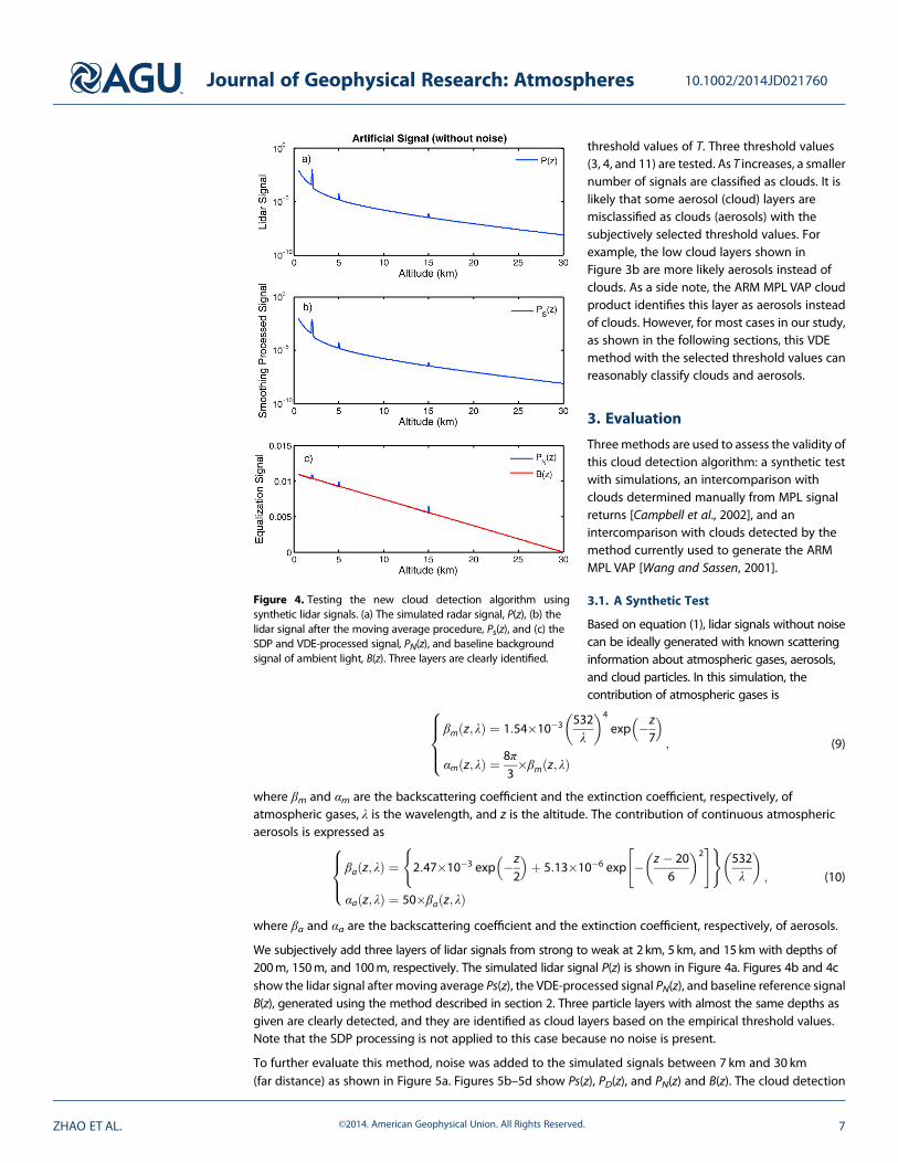
We subjectively add three layers of lidar signals from strong to weak at 2 km, 5 km, and 15 km with depths of200m, 150m, and 100m, respectively. The simulated lidar signal P(z) is shown in Figure 4a. Figures 4b and 4cshow the lidar signal after moving average Ps(z), the VDE-processed signal PN(z), and baseline reference signalB(z), generated using the method described in section 2. Three particle layers with almost the same depths asgiven are clearly detected, and they are identified as cloud layers based on the empirical threshold values.Note that the SDP processing is not applied to this case because no noise is present.

To further evaluate this method, noise was added to the simulated signals between 7 km and 30 km(far distance) as shown in Figure 5a. Figures 5b–5d show Ps(z), PD(z), and PN(z) and B(z). The cloud detection

Figure 4. Testing the new cloud detection algorithm usingsynthetic lidar signals. (a) The simulated radar signal, P(z), (b) thelidar signal after the moving average procedure, Ps(z), and (c) theSDP and VDE-processed signal, PN(z), and baseline backgroundsignal of ambient light, B(z). Three layers are clearly identified.



results show little sensitivity to the noise addedto the simulated signals. The VDE algorithm hasmade all important signal returns detectable.All important layer information has beencaptured in Figures 4 and 5. Noise has beenminimized in the VDE algorithm, and allsudden changes in signals have been includedso that the boundaries of detected particlelayers have a high accuracy. This is essentialbecause some moving average methods cancause changes in particle layer boundaries.

3.2. Evaluation With Lidar Signals FromReal Clouds

As shown in Figure 3, the new algorithm candetect most clouds successfully and identifycloud boundaries accurately, including some thinmultilayer clouds. Even for clouds identifiedduring the noisy period of 1400 to 2300 UniversalTime Coordinates (UT), the new algorithm canstill identify clouds accurately. However, asindicated in section 2.2.3, some layers could bemisclassified due to the threshold values used.For example, the ARM MPL VAP cloud producthas classified the low layers between 0000 and1300 UT as aerosols instead of clouds.

3.3. Comparison With the ARM MPL VAPCloud Product

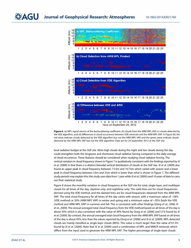
Figure 6 shows MPL backscatteringcoefficients, clouds from the ARM MPL VAP,

clouds generated by the VDE cloud detection algorithm, and differences between the ARMMPLVAP and VDEretrievals on 24 September 2012 at the SGP site. Both algorithms identify similar cloud boundaries, especiallyfor single-layer clouds. However, two major differences are seen. For high-level clouds over low thin clouds,the VDE algorithm can give more continuous and accurate cloud information than can the ARM MPL VAP.Cases on other days also show this. As shown later in Figure 7, statistical results show considerable (~1–3%)differences between two algorithms for high-level clouds. This is consistent with the characteristics of theVDE retrieval algorithmwhich can reduce themagnitude of signal-to-noise variations with distance andmakeit possible for us to identify these clouds located high in the atmosphere. The other major difference is thatcloud bases from the VDE algorithm are generally higher than those from the ARM MPL VAP, and cloud topsfrom the VDE algorithm are generally lower than those from the ARMMPLVAP. This is also consistent with thecharacteristics of VDE retrieval algorithm which keeps sharp signal changes at cloud bases and tops.

4. Results

The new MPL cloud detection algorithm is applied to 1 year of measurements collected at the SGP site andTaihu site. The following shows the cloud detection results and corresponding analyses.

4.1. The SGP Site

As indicated earlier, we consider the measurements made at the SGP site from May 2012 to May 2013.Figure 7 shows the diurnal variation in cloud frequency observed by the MPL using the VDE cloud detectionalgorithm and the ARM MPL cloud product [Wang and Sassen, 2001]. Both retrievals show almost the samediurnal and vertical variations: more clouds occur during the night than during the day; more clouds occurat heights of 3–6 km and 8–12 km during the night; and more clouds occur at heights of 0.5–1.5 km, 3–5 km,and 7–10 km during the day. These diurnal and vertical variations in cloud occurrence are very important for the

Figure 5. Same as Figure 4, but with noise added to the syntheticlidar signals.



local radiative budget at the SGP site. More high clouds during the night and low clouds during the daycould strengthen both the longwave and shortwave cloud radiative forcing compared to the daily averageof cloud occurrence. These features should be considered when studying cloud radiative forcing. Thevertical variation in cloud frequency shown in Figure 7 is qualitatively consistent with the findings reported by Xiet al. [2009] in that there is a distinct bimodal vertical distribution of clouds at the SGP site. Xi et al. [2009] alsofound an upper peak in cloud frequency between 7.5 km and 10.7 km which varied with season and a lowerpeak in cloud frequency between 2 km and 3 km which is lower than what is shown in Figure 7. The differentstudy periodsmay explain this: this study uses data from1 year while Xi et al. [2009] used 10 years of data to carryout their statistical study.

Figure 8 shows the monthly variation in cloud frequency at the SGP site for total, single-layer, and multilayerclouds for all times of the day, daytime only, and nighttime only. The solid lines are for cloud frequenciesderived using the VDE method, and the dashed lines are for cloud frequencies obtained from the ARM MPLVAP. The total cloud frequency for all times of the day varies with season, with a maximum value of ~58%(VDE method) or 50% (ARM MPL VAP) in winter and spring and a minimum value of ~35% (both the VDEmethod and ARM MPL VAP) in summer and fall. This is consistent with other findings [Dong et al., 2006; Xiet al., 2009]. The annual averaged total cloud frequency from the VDE method based on all times of the day isabout 50% which is also consistent with the value of 49% found by Dong et al. [2006] and 51% found by Xiet al. [2009]. By contrast, the annual averaged total cloud frequency from the ARMMPLVAP based on all timesof the day is about 45%, less than the values reported by Dong et al. [2006] and Xi et al. [2009]. MPL-detectedclouds are mainly classified as single-layer clouds (80%). This value is much larger than the value of 61.5%found by Xi et al. [2009]. Note that Xi et al. [2009] used a combination of MPL and MMCR retrievals whichdiffers from the input used to generate the ARM MPL VAP. The higher percentage of single-layer clouds

Figure 6. (a) MPL signal returns of the backscattering coefficient, (b) clouds from the ARM MPL VAP, (c) clouds detected bythe VDE algorithm, and (d) differences in cloud occurrence between VDE retrievals and the ARMMPLVAP. In Figure 6d, thered areas indicate clouds detected by the VDE algorithm but not the ARM MPL VAP, and the green areas indicate cloudsdetected by the ARM MPL VAP but not the VDE algorithm. Data are for 24 September 2012 at the SGP site.



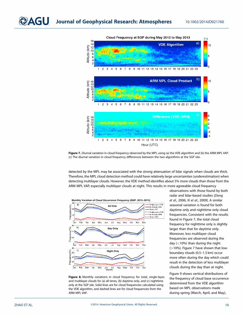
detected by the MPL may be associated with the strong attenuation of lidar signals when clouds are thick.Therefore, the MPL cloud detection method could have relatively large uncertainties (underestimation) whendetecting multilayer clouds. However, the VDE method identifies about 5% more clouds than those from theARM MPL VAP, especially multilayer clouds at night. This results in more agreeable cloud frequency

observations with those found by bothradar and lidar-based studies [Donget al., 2006; Xi et al., 2009]. A similarseasonal variation is found for bothdaytime only and nighttime only cloudfrequencies. Consistent with the resultsfound in Figure 7, the total cloudfrequency for nighttime only is slightlylarger than that for daytime only.Moreover, less multilayer cloudfrequencies are observed during theday (<10%) than during the night(>10%). Figure 7 have shown that low-boundary clouds (0.5–1.5 km) occurmore often during the day which couldresult in the detection of less multilayerclouds during the day than at night.

Figure 9 shows vertical distributions ofthe frequency of cloud base occurrencedetermined from the VDE algorithmbased on MPL observations madeduring spring (March, April, and May),

Figure 7. Diurnal variation in cloud frequency observed by the MPL using (a) the VDE algorithm and (b) the ARMMPL VAP.(c) The diurnal variation in cloud frequency differences between the two algorithms at the SGP site.

Figure 8. Monthly variations in cloud frequency for total, single-layer,and multilayer clouds for (a) all times, (b) daytime only, and (c) nighttimeonly at the SGP site. Solid lines are for cloud frequencies calculated usingthe VDE algorithm, and dashed lines are for cloud frequencies from theARM MPL VAP.



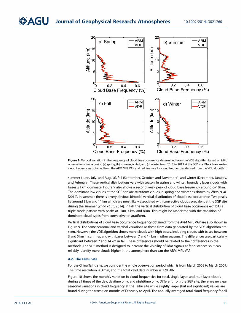
summer (June, July, and August), fall (September, October, and November), and winter (December, January,and February). These vertical distributions vary with season. In spring and winter, boundary layer clouds withbases ≤1 km dominate. Figure 9 also shows a second weak peak of cloud base frequency around 6–10 km.The dominant low clouds at the SGP site are stratiform clouds in spring and winter as shown by Zhao et al.[2014]. In summer, there is a very obvious bimodal vertical distribution of cloud base occurrence. Two peakslie around 3 km and 11 km which are most likely associated with convective clouds prevalent at the SGP siteduring the summer [Zhao et al., 2014]. In fall, the vertical distribution of cloud base occurrence exhibits atriple-mode pattern with peaks at 1 km, 4 km, and 8 km. This might be associated with the transition ofdominant cloud types from convective to stratiform.

Vertical distributions of cloud base occurrence frequency obtained from the ARM MPL VAP are also shown inFigure 9. The same seasonal and vertical variations as those from data generated by the VDE algorithm areseen. However, the VDE algorithm shows more clouds with high bases, including clouds with bases between3 and 5 km in summer, and with bases between 7 and 14 km in other seasons. The differences are particularlysignificant between 7 and 14 km in fall. These differences should be related to their differences in themethods. The VDE method is designed to increase the visibility of lidar signals at far distances so it canreliably identify more clouds higher in the atmosphere than can the ARM MPL VAP.

4.2. The Taihu Site

For the China Taihu site, we consider the whole observation period which is from March 2008 to March 2009.The time resolution is 3min, and the total valid data number is 128,586.

Figure 10 shows the monthly variation in cloud frequencies for total, single-layer, and multilayer cloudsduring all times of the day, daytime only, and nighttime only. Different from the SGP site, there are no clearseasonal variations in cloud frequency at the Taihu site while slightly larger (but not significant) values arefound during the transition months of February to April. The annually averaged total cloud frequency for all

Figure 9. Vertical variation in the frequency of cloud base occurrence determined from the VDE algorithm based on MPLobservations made during (a) spring, (b) summer, (c) fall, and (d) winter from 2012 to 2013 at the SGP site. Black lines are forcloud frequencies obtained from the ARMMPLVAP, and red lines are for cloud frequencies derived from the VDE algorithm.



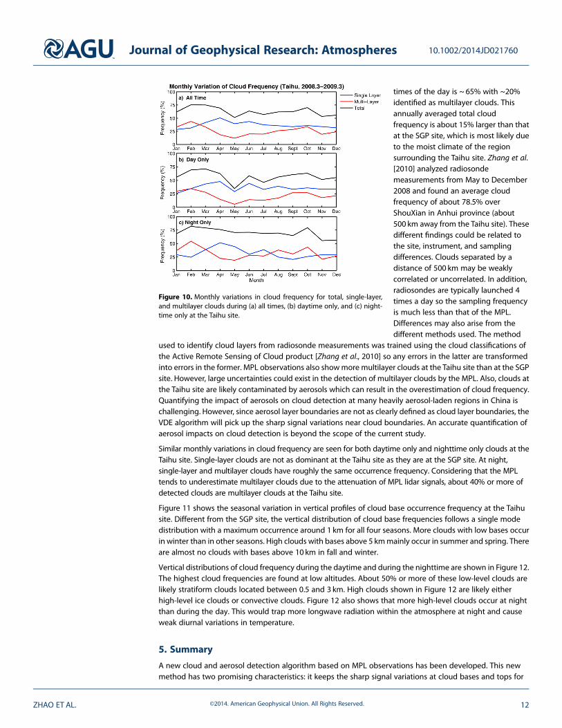
times of the day is ~ 65% with ~20%identified as multilayer clouds. Thisannually averaged total cloudfrequency is about 15% larger than thatat the SGP site, which is most likely dueto the moist climate of the regionsurrounding the Taihu site. Zhang et al.[2010] analyzed radiosondemeasurements from May to December2008 and found an average cloudfrequency of about 78.5% overShouXian in Anhui province (about500 km away from the Taihu site). Thesedifferent findings could be related tothe site, instrument, and samplingdifferences. Clouds separated by adistance of 500 km may be weaklycorrelated or uncorrelated. In addition,radiosondes are typically launched 4times a day so the sampling frequencyis much less than that of the MPL.Differences may also arise from thedifferent methods used. The method

used to identify cloud layers from radiosonde measurements was trained using the cloud classifications ofthe Active Remote Sensing of Cloud product [Zhang et al., 2010] so any errors in the latter are transformedinto errors in the former. MPL observations also showmore multilayer clouds at the Taihu site than at the SGPsite. However, large uncertainties could exist in the detection of multilayer clouds by the MPL. Also, clouds atthe Taihu site are likely contaminated by aerosols which can result in the overestimation of cloud frequency.Quantifying the impact of aerosols on cloud detection at many heavily aerosol-laden regions in China ischallenging. However, since aerosol layer boundaries are not as clearly defined as cloud layer boundaries, theVDE algorithm will pick up the sharp signal variations near cloud boundaries. An accurate quantification ofaerosol impacts on cloud detection is beyond the scope of the current study.

Similar monthly variations in cloud frequency are seen for both daytime only and nighttime only clouds at theTaihu site. Single-layer clouds are not as dominant at the Taihu site as they are at the SGP site. At night,single-layer and multilayer clouds have roughly the same occurrence frequency. Considering that the MPLtends to underestimate multilayer clouds due to the attenuation of MPL lidar signals, about 40% or more ofdetected clouds are multilayer clouds at the Taihu site.

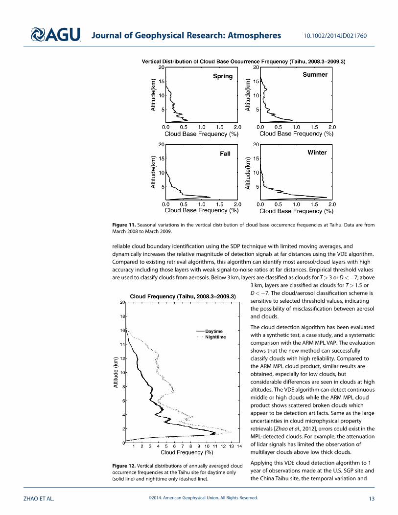
Figure 11 shows the seasonal variation in vertical profiles of cloud base occurrence frequency at the Taihusite. Different from the SGP site, the vertical distribution of cloud base frequencies follows a single modedistribution with a maximum occurrence around 1 km for all four seasons. More clouds with low bases occurin winter than in other seasons. High clouds with bases above 5 kmmainly occur in summer and spring. Thereare almost no clouds with bases above 10 km in fall and winter.

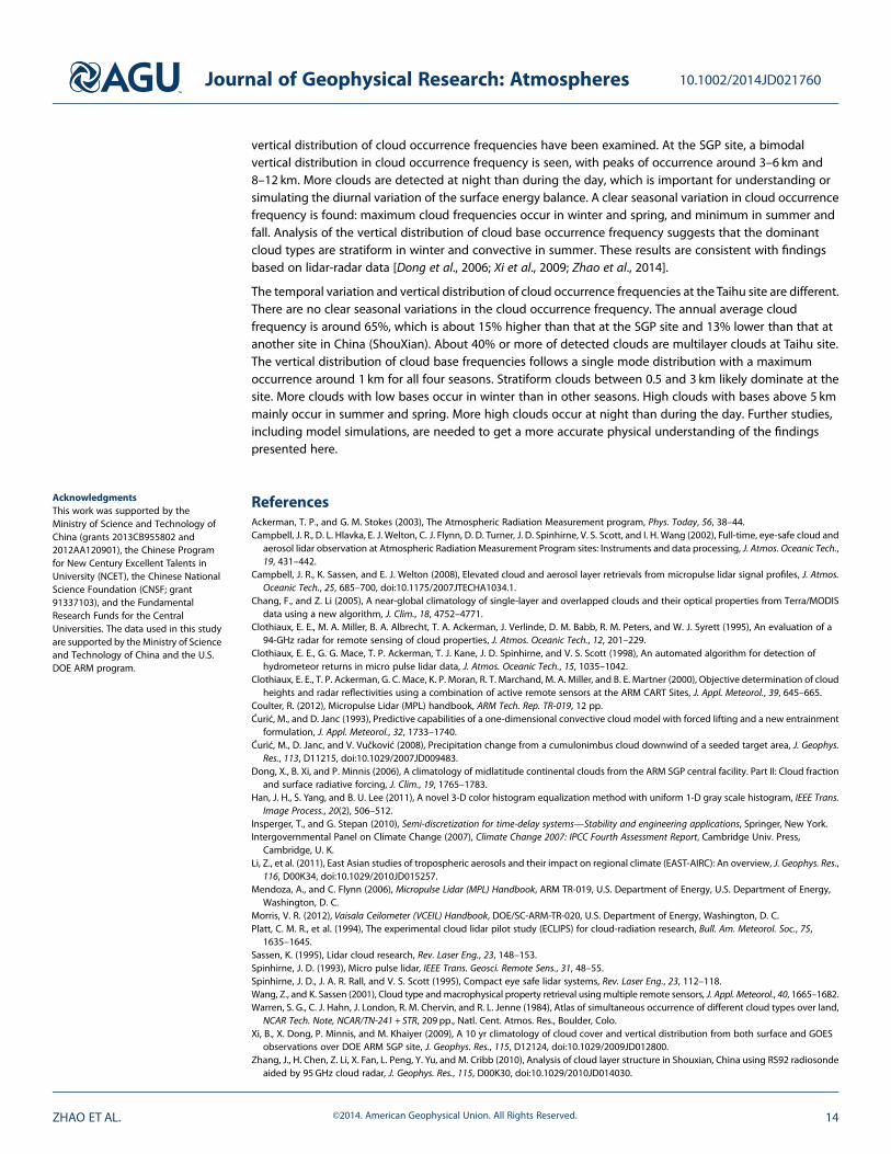
Vertical distributions of cloud frequency during the daytime and during the nighttime are shown in Figure 12.The highest cloud frequencies are found at low altitudes. About 50% or more of these low-level clouds arelikely stratiform clouds located between 0.5 and 3 km. High clouds shown in Figure 12 are likely eitherhigh-level ice clouds or convective clouds. Figure 12 also shows that more high-level clouds occur at nightthan during the day. This would trap more longwave radiation within the atmosphere at night and causeweak diurnal variations in temperature.

5. Summary

A new cloud and aerosol detection algorithm based on MPL observations has been developed. This newmethod has two promising characteristics: it keeps the sharp signal variations at cloud bases and tops for

Figure 10. Monthly variations in cloud frequency for total, single-layer,and multilayer clouds during (a) all times, (b) daytime only, and (c) night-time only at the Taihu site.



reliable cloud boundary identification using the SDP technique with limited moving averages, anddynamically increases the relative magnitude of detection signals at far distances using the VDE algorithm.Compared to existing retrieval algorithms, this algorithm can identify most aerosol/cloud layers with highaccuracy including those layers with weak signal-to-noise ratios at far distances. Empirical threshold valuesare used to classify clouds from aerosols. Below 3 km, layers are classified as clouds for T> 3 or D<�7; above

3 km, layers are classified as clouds for T> 1.5 orD<�7. The cloud/aerosol classification scheme issensitive to selected threshold values, indicatingthe possibility of misclassification between aerosoland clouds.

The cloud detection algorithm has been evaluatedwith a synthetic test, a case study, and a systematiccomparison with the ARM MPL VAP. The evaluationshows that the new method can successfullyclassify clouds with high reliability. Compared tothe ARM MPL cloud product, similar results areobtained, especially for low clouds, butconsiderable differences are seen in clouds at highaltitudes. The VDE algorithm can detect continuousmiddle or high clouds while the ARM MPL cloudproduct shows scattered broken clouds whichappear to be detection artifacts. Same as the largeuncertainties in cloud microphysical propertyretrievals [Zhao et al., 2012], errors could exist in theMPL-detected clouds. For example, the attenuationof lidar signals has limited the observation ofmultilayer clouds above low thick clouds.

Applying this VDE cloud detection algorithm to 1year of observations made at the U.S. SGP site andthe China Taihu site, the temporal variation and

Figure 11. Seasonal variations in the vertical distribution of cloud base occurrence frequencies at Taihu. Data are fromMarch 2008 to March 2009.

Figure 12. Vertical distributions of annually averaged cloudoccurrence frequencies at the Taihu site for daytime only(solid line) and nighttime only (dashed line).



vertical distribution of cloud occurrence frequencies have been examined. At the SGP site, a bimodalvertical distribution in cloud occurrence frequency is seen, with peaks of occurrence around 3–6 km and8–12 km. More clouds are detected at night than during the day, which is important for understanding orsimulating the diurnal variation of the surface energy balance. A clear seasonal variation in cloud occurrencefrequency is found: maximum cloud frequencies occur in winter and spring, and minimum in summer andfall. Analysis of the vertical distribution of cloud base occurrence frequency suggests that the dominantcloud types are stratiform in winter and convective in summer. These results are consistent with findingsbased on lidar-radar data [Dong et al., 2006; Xi et al., 2009; Zhao et al., 2014].

The temporal variation and vertical distribution of cloud occurrence frequencies at the Taihu site are different.There are no clear seasonal variations in the cloud occurrence frequency. The annual average cloudfrequency is around 65%, which is about 15% higher than that at the SGP site and 13% lower than that atanother site in China (ShouXian). About 40% or more of detected clouds are multilayer clouds at Taihu site.The vertical distribution of cloud base frequencies follows a single mode distribution with a maximumoccurrence around 1 km for all four seasons. Stratiform clouds between 0.5 and 3 km likely dominate at thesite. More clouds with low bases occur in winter than in other seasons. High clouds with bases above 5 kmmainly occur in summer and spring. More high clouds occur at night than during the day. Further studies,including model simulations, are needed to get a more accurate physical understanding of the findingspresented here.

ReferencesAckerman, T. P., and G. M. Stokes (2003), The Atmospheric Radiation Measurement program, Phys. Today, 56, 38–44.Campbell, J. R., D. L. Hlavka, E. J. Welton, C. J. Flynn, D. D. Turner, J. D. Spinhirne, V. S. Scott, and I. H. Wang (2002), Full-time, eye-safe cloud and

aerosol lidar observation at Atmospheric Radiation Measurement Program sites: Instruments and data processing, J. Atmos. Oceanic Tech.,19, 431–442.

Campbell, J. R., K. Sassen, and E. J. Welton (2008), Elevated cloud and aerosol layer retrievals from micropulse lidar signal profiles, J. Atmos.Oceanic Tech., 25, 685–700, doi:10.1175/2007JTECHA1034.1.

Chang, F., and Z. Li (2005), A near-global climatology of single-layer and overlapped clouds and their optical properties from Terra/MODISdata using a new algorithm, J. Clim., 18, 4752–4771.

Clothiaux, E. E., M. A. Miller, B. A. Albrecht, T. A. Ackerman, J. Verlinde, D. M. Babb, R. M. Peters, and W. J. Syrett (1995), An evaluation of a94-GHz radar for remote sensing of cloud properties, J. Atmos. Oceanic Tech., 12, 201–229.

Clothiaux, E. E., G. G. Mace, T. P. Ackerman, T. J. Kane, J. D. Spinhirne, and V. S. Scott (1998), An automated algorithm for detection ofhydrometeor returns in micro pulse lidar data, J. Atmos. Oceanic Tech., 15, 1035–1042.

Clothiaux, E. E., T. P. Ackerman, G. C. Mace, K. P. Moran, R. T. Marchand, M. A. Miller, and B. E. Martner (2000), Objective determination of cloudheights and radar reflectivities using a combination of active remote sensors at the ARM CART Sites, J. Appl. Meteorol., 39, 645–665.

Coulter, R. (2012), Micropulse Lidar (MPL) handbook, ARM Tech. Rep. TR-019, 12 pp.Ćurić, M., and D. Janc (1993), Predictive capabilities of a one-dimensional convective cloud model with forced lifting and a new entrainment

formulation, J. Appl. Meteorol., 32, 1733–1740.Ćurić, M., D. Janc, and V. Vučković (2008), Precipitation change from a cumulonimbus cloud downwind of a seeded target area, J. Geophys.

Res., 113, D11215, doi:10.1029/2007JD009483.Dong, X., B. Xi, and P. Minnis (2006), A climatology of midlatitude continental clouds from the ARM SGP central facility. Part II: Cloud fraction

and surface radiative forcing, J. Clim., 19, 1765–1783.Han, J. H., S. Yang, and B. U. Lee (2011), A novel 3-D color histogram equalization method with uniform 1-D gray scale histogram, IEEE Trans.

Image Process., 20(2), 506–512.Insperger, T., and G. Stepan (2010), Semi-discretization for time-delay systems—Stability and engineering applications, Springer, New York.Intergovernmental Panel on Climate Change (2007), Climate Change 2007: IPCC Fourth Assessment Report, Cambridge Univ. Press,

Cambridge, U. K.Li, Z., et al. (2011), East Asian studies of tropospheric aerosols and their impact on regional climate (EAST-AIRC): An overview, J. Geophys. Res.,

116, D00K34, doi:10.1029/2010JD015257.Mendoza, A., and C. Flynn (2006), Micropulse Lidar (MPL) Handbook, ARM TR-019, U.S. Department of Energy, U.S. Department of Energy,

Washington, D. C.Morris, V. R. (2012), Vaisala Ceilometer (VCEIL) Handbook, DOE/SC-ARM-TR-020, U.S. Department of Energy, Washington, D. C.Platt, C. M. R., et al. (1994), The experimental cloud lidar pilot study (ECLIPS) for cloud-radiation research, Bull. Am. Meteorol. Soc., 75,

1635–1645.Sassen, K. (1995), Lidar cloud research, Rev. Laser Eng., 23, 148–153.Spinhirne, J. D. (1993), Micro pulse lidar, IEEE Trans. Geosci. Remote Sens., 31, 48–55.Spinhirne, J. D., J. A. R. Rall, and V. S. Scott (1995), Compact eye safe lidar systems, Rev. Laser Eng., 23, 112–118.Wang, Z., and K. Sassen (2001), Cloud type andmacrophysical property retrieval usingmultiple remote sensors, J. Appl. Meteorol., 40, 1665–1682.Warren, S. G., C. J. Hahn, J. London, R. M. Chervin, and R. L. Jenne (1984), Atlas of simultaneous occurrence of different cloud types over land,

NCAR Tech. Note, NCAR/TN-241 + STR, 209 pp., Natl. Cent. Atmos. Res., Boulder, Colo.Xi, B., X. Dong, P. Minnis, and M. Khaiyer (2009), A 10 yr climatology of cloud cover and vertical distribution from both surface and GOES

observations over DOE ARM SGP site, J. Geophys. Res., 115, D12124, doi:10.1029/2009JD012800.Zhang, J., H. Chen, Z. Li, X. Fan, L. Peng, Y. Yu, and M. Cribb (2010), Analysis of cloud layer structure in Shouxian, China using RS92 radiosonde

aided by 95GHz cloud radar, J. Geophys. Res., 115, D00K30, doi:10.1029/2010JD014030.



AcknowledgmentsThis work was supported by theMinistry of Science and Technology ofChina (grants 2013CB955802 and2012AA120901), the Chinese Programfor New Century Excellent Talents inUniversity (NCET), the Chinese NationalScience Foundation (CNSF; grant91337103), and the FundamentalResearch Funds for the CentralUniversities. The data used in this studyare supported by the Ministry of Scienceand Technology of China and the U.S.DOE ARM program.

Zhang, Z., Z. Li, H. Chen, and M. Cribb (2013), Validation of a radiosonde-based cloud layer retrieval method using ground-based remotesensing methods at multiple ARM sites, J. Geophys. Res. Atmos, 118, 846–858, doi:10.1029/2012JD018515.

Zhao, C., et al. (2012), Toward understanding of differences in current cloud retrievals of ARM ground-based measurements, J. Geophys. Res.,117, D10206, doi:10.1029/2011JD016792.

Zhao, C., S. Xie, X. Chen, M. P. Jensen, and M. Dunn (2014), Quantifying uncertainties of cloud microphysical property retrievals with aperturbation method, J. Geophys. Res. Atmos., 119, 5375–5385, doi:10.1002/2013JD021112.



Documents

PUBLICATIONS - University Of Marylandzli/PDF_papers/Zhao_et_al_jgrd...Jiangsu province in China and was in operation during the East Asian Study of Tropospheric Aerosols and Impact