Embed Size (px)
Citation preview
PUBLIC VERSION
Master Thesis Forecasting promotional demand in the
FMCG industry
September 4, 2020
Tom Weustink s1726587
Study: Industrial Engineering and Management (MSc)
Specialization: Production & Logistics Management
Company: Grolsch Bierbrouwerij N.V.
Department: Demand Planning
Supervisor UT: dr. ir. M.R.K. Mes
Supervisor UT: dr. E. Topan
Supervisor Grolsch: Peter Bouwhuis

2
All confidential information in this public version is anonymized by:
- Dividing the value with a fixed number known by the author. - Deleting axes, figures, or tables - Removing sensitive paragraphs or appendices
3
Management Summary This research is conducted at the department demand planning & customer service at Royal Grolsch N.V.
in Enschede. Grolsch is a Dutch manufacturer that produces beer from raw materials to end products. The
company divides its sales into the sales categories on-trade, off-trade, and business development.
The demand planning department observes that the current demand planning process results in a high
workload, and continuous quick fixes to meet deadlines and to obtain a good forecast. They believe that
the process could be improved to achieve a higher efficiency, increased effectiveness, and an increased
forecast accuracy by standardization. In the current situation, they forecast mainly on the total demand
level, but they desire to distinguish a forecast for baseline demand and promotional demand. The baseline
demand is the demand during a period when there is no promotion. The current baseline demand is
determined by a computer, but the demand planning identified that these baselines are not reliable.
Therefore, they want an own method to determine the baseline demand, which is based on historical sales
data.
Besides, promotions have become more and more important for Grolsch during the last years. In total, 70
– 80 percent of the total volume is sold during promotion. The promotional volume is the difference
between realized sales of a promotion and the baseline demand, and it is influenced by numerous factors.
Currently, it is known which factors influence the promotional volume, but the impact of each variable is
unknown. The current promotional forecast is based on experience, sales, and human knowledge. They
are determined by the customer support employees, and each employee has their forecasting method.
Because many stakeholders are involved in the demand planning process, there are often the same
discussions about the promotional volume. The reason for this is that the impact of each variable is
unknown and because there is no standardized method for determining the promotional demand.
Therefore, the objective of this research is:
Developing a standardized method for determining baseline demand based on historical data, and to
create a model for forecasting the promotional volume. It should contain well-founded assumptions and
it provides insight into the relations between variables that impact the promotional volume.
We start this research by developing a method for establishing the baseline sales. We use the historic sales
data as input, and we clean this data for promotions, weather, and outliers to obtain the baseline sales.
The total sales are cleaned for these factors because they do not belong to base demand. The method is
implemented with Excel VBA. After cleaning the total sales, we obtain the baseline sales from previous
years, and we use them to determine the promotional volume for each promotion.
We found in literature that a widespread approach for promotional forecasting is the baseline-uplift
method. This method forecasts the promotional volume by multiplying the baseline with an uplift factor.
We conclude that this method is not suitable for Grolsch, and therefore we dive deeper into the field of
machine learning. From literature and evaluating the performance of several machine learning techniques,
we decide that a Random Forest model is most suitable for this research. The reason for this is that a
Random Forest can deal with categorical variables, and we have many categorical variables in our dataset.
This research focusses on off-trade sales because this promotion category has the highest promotion
pressure, and it accounts for the largest sales volume. We use the historical promotions from 2017 – 2019
as input for the analysis. The promotions that do not need a forecast are removed from the dataset, and
it is cleaned for outliers and missing values. To select the variables that have the highest predictive power,

4
we use a feature selection method in combination with tree-based regression methods. From this analysis,
we conclude that account, product code, month, price, and promotion mechanism are the variables with
the highest impact for predicting the promotional volume. We conduct 25 experiments to find the optimal
input parameters for the Random Forest. The most important predictors and the optimal input
configuration are used as input for the final model.
We assign all product codes to a promotion category to measure the forecast accuracy, and we use the
MAD, MAPE, RMSE, and wMAPE as performance indicators. 5-fold cross-validation is applied to validate
the results. We found in this research that using a subset of the input data can result in higher forecasting
performance for a specific promotion category. Therefore, three different subsets are created and tested
on each promotion category to create the final model. For the final model, we use the dataset that has the
highest performance for a promotion category. We conclude that the highest performance is achieved for
the promotion categories GPP Crate, GPP Can, Grolsch Summer, Lentebok, and Craft-beer if we use only
the data for that specific category as an input. For the other promotion categories, we achieve the highest
performance if the dataset without Grolsch Premium Pilsner promotions is used. The reason for this is that
there are large differences between the promotional volumes of different products and retailers. The
performance of the current forecasting method and the final prediction model are presented in Table M1
and Table M2 respectively.
Table M1 | Performance promotion models for a single promotion category (Current = Current Method, RF = Random Forest Model)
Performance measure
GPP Crate GPP Can Grolsch Summer Lentebok Craft-beer
Current RF Current RF Current RF Current RF Current RF
MAD 286 257 94 82 52 48 37 40 11 11
MAPE 36% 33% 24% 29% 82% 77% 50% 79% 70% 115%
RMSE 674 603 218 181 107 101 58 63 16 16
wMAPE 19% 17% 31% 27% 96% 41% 37% 39% 55% 54%
Table M2 | Performance promotion model for dataset without GPP (Current = Current Method, RF = Random Forest Model)
Performance measure
Grimbergen Kornuit Other Kornuit Crate Low-Promo Herfstbok
Current RF Current RF Current RF Current RF Current RF
MAD (HL) 46 34 46 41 214 158 45 30 91 69
MAPE (%) 64% 70% 61% 67% 68% 50% 41% 37% 87% 68%
RMSE (HL) 96 70 75 63 317 228 89 65 194 137
wMAPE (%) 47% 12% 38% 8% 50% 37% 40% 27% 50% 26%
The performance indicators that score better are marked green in Table M1 and Table M2, and the
performance indicator that performs worse are marked red. We conclude from these tables that the
Random Forest model shows for most promotion categories an improvement or it performs similar to the
current method. Some promotion categories perform worse than the current forecasting method, such as
craft-beer and Lentebok. A reason for this could be that the promotion category craft-beer has not much
observations, and the promotional volumes of Lentebok have large fluctuations due to seasonality
patterns, which makes it difficult to forecast. Another conclusion is that the model performs better for
large promotional volumes than low promotional volumes. The wMAPE puts a higher weight on
promotions with large sales volumes. The consequence is that if we make a better prediction for a large

5
promotional volume, it has more impact on the forecast error than a prediction for a low promotional
volume. Because the wMAPE is for most categories lower than the regular MAPE, we conclude that the
model has a better forecast accuracy for large sales volumes. This model can be used as an extra decision
tool for forecasting promotional volumes. The results are implemented in an Excel Tool that can be used
for promotional forecasting. The Random Forest model and the Excel tool standardize the promotional
forecasting process.
In the end of this reserach, we study the impact of the forecasting model on the costs for the safety stock
of Grolsch Premium Pilsner. This analysis is based on the forecasts and sales of 2019. The current
promotional volumes are replaced with the volumes according to the prediction model. From this, we
conclude that the forecasting model results in a decrease of XX HL for the standard deviation of weekly
demand. The demand for this product is normal distributed, which allows us to apply a safety stock model
for the fill rate. We test the old and new standard deviation for the same fill rate model. We conclude from
this that the safety stock could be reduced with 2.5 percent with a potential saving of XX euros per year
while maintaining the same fill rate of XX percent.

6
Preface This report presents the thesis ‘Forecasting Promotional Demand in the FMCG Industry’. The research is
conducted at Royal Grolsch to finish my master’s in Industrial Engineering & Management at the University
of Twente.
The first month I worked at Grolsch where I gained much knowledge about promotional forecasting.
However, after the first month I needed to continue my thesis from home due to the corona virus. I would
like to thank all employees from Grolsch who assisted me with the research and for the good experience
despite the strange circumstances. I would like to thank Ferran Ruiz for offering me this interesting
assignment, and Koen Oost and Peter Bouwhuis for their support during the research even though their
busy schedules.
Besides, I would like to thank Martijn Mes and Engin Topan from the University of Twente for supervising
me and their feedback. Their critical view helped me structuring the report and delivering a better product.
Tom Weustink
Denekamp, September 2020

7
List with figures
Figure Description
1.1 Problem Cluster
1.2 Stakeholder of the research
2.1 Promotional planning process
2.2 Sell in and Sell out demand
2.3 Division of demand types
2.4 Sell-in sales volume
2.5 Sell-out sales volume
3.1 5-fold Cross-Validation
4.1A Cleaning the total sales to obtain baseline sales per product-retailer
4.1B Pseudo code promotion impact after promotion week n
4.2 Logic of promotion cleaning
5.1 Histogram of the promotional volume of all promotions
5.2 Histogram of promotional volume for all promotions except GPP
5.3A Relation between price and uplift for GPP crates
5.3B Frequencies of each level for multibuy1, multibuy2, and multibuy3
5.4 Level of retailer competition for Grolsch Premium Pilsner
5.5 Levels of attribute brewery1 - Competitors of Grolsch Premium Pilsner (GPP) that have a promotion in the same week
5.6 Levels of attribute brewery2 - GPP competitors that have a promotion at the same retailer in the same week
5.7 Levels of attribute brewery3 - GPP promotions that have a promotion in the same week
6.1 Results of feature selection
6.2 Results experiments of ntree and mtry
6.3 Variable importance of RandomForest using %IncMSE
7.1 Screenshot of Excel tool for promotional forecasting (forecast intentionally left blank)
7.2 Histogram of weekly demand for product A in 2019
7.3 QQ plot of weekly demand for product A in 2019

8
List with tables
Table Description
M1 Performance promotion models for a single promotion category
M2 Performance promotion model for dataset without GPP
3.1 Results literature overview of Gupta & Van Heerde (2005)
4.1 Difference between ex-brewery and IRI-data
4.2 The impact of one ADS-day on the average increase in baseline sales (%)
4.3 (raw) ex-brewery sales data and cleaned baseline for Grolsch Premium Pilsner Product A
5.1 Data sources that are used for analysis
5.2 Cleaning of promotional database
5.3A Volume (percentage/hectoliter) and as a percentage of the total number of promotions.
5.3B Minimum, average, and maximum volume per product-retailer
5.4 List with promotional factors
5.5 Variables used for promotion mechanism
5.6 Level of competition for Grolsch Premium Pilsner (1 = high, 5 = low)
5.7 matrix that combines retailer and brewery competition (brewery competition type 3)
5.8 categories with temperature ranges
5.9 Total baseline sales (hector liter) per promotion category in 2019
6.1 Linear model for predicting the uplift and promotional volume
6.2 Results several machine learning algorithms RapidMiner
6.3 Experimental factors
6.4 Results of feature selection on the complete dataset.
6.5 Variables that are chosen in each experiment – all promotions
6.6 Results feature selection on the complete dataset.
6.7 Variables that are chosen in each experiment – all promotions except GPP
6.8 Results feature selection on complete GPP dataset
6.9 Variables that are chosen in each experiment – all GPP promotions
6.10 Performance promotion models for a single category (Current = Current Method, RF = Random Forest Model)
6.11 Performance promotion model for dataset without GPP (Current = Current Method, RF = Random Forest Model)
7.1 MAD and standard deviation of demand for the current forecasting method and Random Forest model
7.2 Input for calculation
7.3 Results safety stock analysis
C1 Performance promotion models for a single promotion category
C2 Performance promotion model for dataset without GPP

9
Contents Management Summary ................................................................................................................................. 2
Preface ........................................................................................................................................................... 6
List with figures ............................................................................................................................................. 7
List with tables ............................................................................................................................................... 8
Chapter 1 | Introduction ............................................................................................................................. 11
1.1 Company Introduction ...................................................................................................................... 11
1.2 Problem introduction ........................................................................................................................ 11
1.3 Stakeholders ...................................................................................................................................... 15
1.4 Research Framework ......................................................................................................................... 16
1.5 Scope ................................................................................................................................................. 17
Chapter 2 | Current situation ...................................................................................................................... 19
2.1 Promotional planning ........................................................................................................................ 19
2.2 Demand Planning .............................................................................................................................. 20
2.3 Conclusion ......................................................................................................................................... 23
Chapter 3 | Literature review...................................................................................................................... 25
3.1 The impact of promotions on demand.............................................................................................. 25
3.2 Factors that influence promotion effectivity .................................................................................... 26
3.3 Forecasting promotional volumes in the FMCG industry.................................................................. 28
3.4 Developing a prediction model ......................................................................................................... 29
3.5 Performance of a prediction model .................................................................................................. 32
3.6 Validating a prediction model ........................................................................................................... 35
3.7 Conclusion ......................................................................................................................................... 37
Chapter 4 | Baseline calculation ................................................................................................................. 39
4.1 Introduction ....................................................................................................................................... 39
4.2 Input for determining the baseline sales .......................................................................................... 40
4.3 Cleaning process ................................................................................................................................ 40
4.4 Results ............................................................................................................................................... 43
4.5 Forecasting baseline demand ............................................................................................................ 44
4.6 Conclusion ......................................................................................................................................... 45
Chapter 5 | Data Preparation & preliminary analysis ................................................................................. 47
5.1 Data acquisition ................................................................................................................................. 47
5.2 Data cleaning ..................................................................................................................................... 48

10
5.3 Distribution of promotional volumes ................................................................................................ 49
5.4 Variables ............................................................................................................................................ 50
5.5 Promotion categories ........................................................................................................................ 57
5.6 Performance indicators ..................................................................................................................... 58
5.7 Conclusion ......................................................................................................................................... 59
Chapter 6 | Results ...................................................................................................................................... 61
6.1 Multiple Linear Regression ................................................................................................................ 61
6.2 Machine learning methods................................................................................................................ 62
6.3 Feature selection ............................................................................................................................... 63
6.4 Random Forest – Optimization of input parameters ........................................................................ 67
6.5 Forecasting model ............................................................................................................................. 68
6.6 Conclusion ......................................................................................................................................... 70
Chapter 7 | Implementation of the framework .......................................................................................... 71
7.1 Impact of research for demand planning .......................................................................................... 71
7.2 Forecasting tool ................................................................................................................................. 72
7.3 Impact of forecast accuracy on operations ....................................................................................... 73
7.4 Conclusion ......................................................................................................................................... 78
Chapter 8 | Conclusion, Discussion & Recommendations .......................................................................... 79
8.1 Conclusion ......................................................................................................................................... 79
8.2 Discussion .......................................................................................................................................... 81
8.3 Recommendations............................................................................................................................. 83
References ................................................................................................................................................... 85
Appendices .................................................................................................................................................. 87

11
Chapter 1 | Introduction In this chapter, we provide an introduction to Koninklijke Grolsch in Section 1.1. The research motivation
and the problem are introduced in Section 1.2. This is followed by the stakeholders of the research (Section
1.3). We close this chapter with the research framework (Section 1.4) and the scope of the research
(Section 1.5).
1.1 Company Introduction This research is conducted at the department demand planning & customer service at Royal Grolsch N.V.
Since 2016, the company is part of Asahi Group Holdings, which is a Japanese beer manufacturer. Grolsch
brews their beer from raw-material to end-product. The company does not only produce their own brands,
but it also produces beer for other companies such as Peroni, Grimbergen, and Lech. XX percent of the
products are sold nationally, and XX percent of the products are sold internationally.
Grolsch divides its sales into three categories: on-trade, off-trade, and business development. These
divisions are accountable for XX percent, XX percent, and XX percent of the total sales volume respectively.
On-trade is responsible for hospitality and wholesale, off-trade is responsible for retail, and business
development procures beer from other manufacturers and sells them to other businesses. The demand
planning department is responsible for the forecast for the short and long-term in collaboration with the
other departments.
1.2 Problem introduction The demand planning department has some structural challenges at several stages of the forecasting
process, which we introduce in this section. We describe the motivation for the research (Section 1.2.1).
We conduct interviews with different employees to identify all possible problems. These problems are
elaborated in a problem cluster using the Managerial Problem-Solving Method (Heerkens & Van Winden,
2017). This resulted in the problem identification (Section 1.2.2).
1.2.1 Research motivation Promotions have become more and more important for Grolsch during the last years. In total, Grolsch sells
70-80 percent of the total national sales volume during promotions. Since Grolsch is a manufacturer within
the fast-moving consumer goods (FMCG) market, there is a high demand for product availability (Basson,
Kilbourn, & Walters, 2019). Therefore, it is important to have a high forecast accuracy such that processes
are organized efficiently to obtain this high product availability.
Grolsch uses forecasting on several management levels. Forecasting is needed at a strategic level to
evaluate growth opportunities, and to establish plans for the upcoming years together with sales and
marketing. Forecasting is needed at a tactical and operational level to create efficient and effective
operations. An example is that inventories are used to guarantee high service levels. When inventories are
too high, then products might become obsolete resulting in high costs. When inventories are too low, then
products can go out-of-stock, which results in lost-sales, penalties, and unsatisfied customers. Therefore,
a good forecast is needed to prevent these situations.

12
Demand management is a process that consists of several steps in creating accurate forecasts (Lucia et al.,
2017). It is about balancing the supply chain capabilities with the requirements of the customers, which
involves forecasting demand and integrating it with production, procurement, and distribution
capabilities. It is one of the most important factors in improving the efficiency of operations (Croxton et
al., 2002).
Adebanjo & Mann (2000) describe the main advantages of having a good forecast. They state that a good
forecast increases product availability to the customers, reduces inventory levels in supply chains, results
in more effective use of capital assets, provides clearer identification of capital needs in the future and it
improves customer/supplier relationships. Croxton et al. (2002) state that lowering the demand variability
results in more consistent planning, fewer costs, smoother operations, and higher flexibility.
The current demand planning process results in a high workload and continuously quick fixes to meet
deadlines and obtain a good forecast. They believe that the process could be improved to achieve a higher
efficiency, more effectivity, and an increased forecast accuracy. In Section 1.2.2, we discuss the issues that
occur at the demand planning department in more detail. The relations between problems are shown in a
problem cluster (Figure 1.1).
1.2.2 Problem description Grolsch distinguishes the total demand in four layers: standard (base) demand, promotional demand, new
product development (NPD), and market insights (MI). Baseline demand represents the sales in a period
when there are no promotions and promotional demand is the demand that results from promotions. The
promotional demand is a quantity on top of the baseline demand and therefore it is difficult to say what
part of the total sales is baseline or promotional demand. Besides, both types of demand are influenced
several factors such as weather and events (holidays). Although baseline and promotional demand are
easy to understand by definition, it is hard to determine it. The demand-planning department faces that
the current baseline sales are often not reliable because there is no standardized method. Therefore, we
need a method to determine which part of the sales belongs to baseline sales and promotional sales.
Dividing the sales into baseline and promotional sales is often-used approach in literature (Cooper, Baron,
Levy, Swisher, & Gogos, 1999; Van Der Poel, 2010; Van Donselaar, Peters, De Jong, & Broekmeulen, 2016).
The layer new product development is the demand from the introduction of new products, and market
insights is about extra demand that arises from marketing activities. We describe the layers in more detail
in Section 2.2.
The demand planning process at Grolsch is divided into several sub-processes. One of these processes is
the demand-review meeting (DRM), in which they discuss monthly the sales volumes, financial budgets,
and whether they are on schedule to meet the sales targets. They evaluate the targets by using the realized
sales and the forecast for the upcoming period. Therefore, Grolsch needs to have a reliable forecast to
evaluate whether they are going to achieve the targets. When the expected sales do not meet the targets,
then Grolsch undertakes actions to increase sales. In the current situation, Grolsch forecasts mainly on
‘total demand level’ instead of the four separate layers, and there is no clear distinction between layers.
Grolsch desires to have more insight into the different demand layers such that they can specify concrete
actions when targets are not achieved. In this research, we focus on the base demand and promotional
demand layer.

13
Promotions, often referred to as trade promotions, become more important in the consumer market
(Ramanathan & Muyldermans, 2010). Often a multiple of the baseline demand is sold during promotions,
which is defined as the lift-factor (realized sales divided by baseline sales). It is difficult to estimate the lift-
factor because of the number of variables and the lack of information. As first, the lift-factor is influenced
by numerous factors, such as price, type of promotion, timing of promotion, execution of promotion,
weather, and promotions of competitors. However, it is not known to what extent each variable impacts
the promotion effectivity, and whether there are more significant factors. Because there is no insight into
the impact of variables, it is difficult to estimate the lift-factor for a promotion. Secondly, there is a lack of
information. Grolsch is prohibited by law to determine the price for a promotion or to know from other
beer companies when they have a promotion. Grolsch can only advise the retailers about the price, after
which the retailer determines the final price. Therefore, the only information that is known at Grolsch is
the week of promotion, type of promotion, and at which retailers there is a Grolsch promotion. Due to the
lack of information and the many variables, Grolsch desires to have more insight into the variables that
influence promotions, because then it is easier to decide which actions/promotions can be taken to meet
sales, and to make a forecast.
Currently, the customer support employees determine the forecast for promotional volumes (Section 1.3),
and they base them on historical data, human knowledge, and experience. These forecasts are evaluated
by the demand planning department, after which they are used as input for the total forecast. Each
employee has their own forecasting method and estimates the promotional volume ad hoc. Since multiple
stakeholders are involved in the demand forecasting process, it often results in the same discussions and
disagreements between stakeholders about the forecasts. These disagreements need to be solved by
reviewing and improving the forecasts. This process takes a lot of time due to many product-retailer
combinations, no standard assumptions, and a lack of insight in the promotion effectivity. All these steps
make the current forecasting process not effective, not efficient and it does not result in the desired
forecast accuracy for some products or retailers.
The main reason for all these problems is that there is no standardized method that can be used for
determining the baseline demand and for forecasting promotional demand. We defined for this research
the following problem statement:
Grolsch does not have a standardized method for determining the baseline sales and forecasting
promotional demand.
The goal of this research is to determine a method for determining baseline sales and to create a model
for predicting the promotional volume and specifying concrete actions with all stakeholders. It contains
well-founded assumptions, and it provides insight into the relations between variables that impact the
promotional volume. This should result in better forecast accuracy and a more structured DRM process.
Besides, demand planning desires that the framework should increase the confidence of stakeholders by
arguments that are based on data.

14
Figure 1.1 | Problem Cluster

15
Figure 1.2 | Stakeholders of the research
1.3 Stakeholders Four stakeholders are involved in this research, which are the following departments: demand planning,
off-trade sales, revenue management, and supply chain planning (Figure 1.2). The first stakeholder is the
demand planning department who initiated this research. They are the problem-owner and are
responsible for combining all information into a long-term and short-term forecast. Their objective is to
standardize the process and to achieve a high forecast accuracy. They desire to receive input from the
different stakeholders such that they can combine it in the total forecast. Besides, demand planning is one
of the end-users of the models.
The second stakeholder in this project is the off-trade sales department. This department consists of
account managers and customer support employees. Each year, Grolsch establishes for each account sales
targets based on the forecast. The account managers are responsible for the sales within the retail
department and achieving these targets. They need to have a reliable forecast to evaluate the
performance of the accounts, and whether the targets are reached. If these goals are not met, then the
account managers can agree with the retailers for extra promotions to increase sales. The employees of
customer support assist account management, and they process the promotions into the system. Besides,
they make a prediction of the promotion volume based on historical data, experience, human knowledge,
and information from the account managers. The framework that we develop should make it easier to
create a forecast, it structures the process and it can be used as a reference for the promotional volume.
The third stakeholder is the revenue management department. This department analyzes projects and
possible actions that yield the most revenue. It uses the forecasts to evaluate the total expected sales,
which can be used for strategic purposes. Besides, this department has conducted some research into
promotion-effectivity. They analyzed the effect of having more promotions, the most favorable
competitors during a promotion, and the best weeks in the year to have a promotion. They have data and
knowledge that is relevant for this research and therefore they are a stakeholder to the research.
The last stakeholder in this research is the supply chain planning department, which is an indirect
stakeholder. They use the total forecast as input for production planning. In the current situation, the
forecast is weekly updated and can have large fluctuations. This makes it difficult for the supply chain
department to create an optimal production plan to achieve efficient operations. Therefore, they desire
to have a short and long-term forecast that has a high accuracy and that does not have a large variability
between weeks.

16
1.4 Research Framework We define several research questions to find a solution to the objective. In this section, we provide the
description and motivation for the research questions. We divide the research questions into five
categories:
1. The current processes of promotional and demand planning
2. Promotional forecasting
3. Modelling decisions
4. Developing and validating the framework
5. Implementing the framework in the demand-planning process
1.4.1 Current processes We need to know how the current process is organized before we can make improvements. The process
for forecasting promotional volumes consists of two processes: demand planning and promotional
planning. Therefore, we propose the following research questions:
1. How is the promotional planning for off-trade organized at Grolsch?
2. How is the total demand at Grolsch defined?
1.4.2 Promotional forecasting The impact of a promotion on the promotional volume is caused by many variables. Grolsch knows which
variables have an impact on the demand, but they do not know whether the list with factors is complete.
Therefore, we need to know more about the effect of promotions, and what is already known in the
literature about variables that influence the promotional volume. Besides, several techniques can be used
to estimate the promotional volume. In this part, we conduct a literature review to investigate what is
already know about promotional forecasting. Therefore, we propose the following research questions:
3. How do promotions impact demand in the FMCG industry?
4. What methods are proposed in the literature for forecasting promotional volumes in the FMCG?
5. What factors influence promotion effectivity in the FMCG according to literature?
1.4.3 Modelling decisions One of the main objectives of this research is to gain more insight into the effects of promotion on the lift-
factor and promotional volume. We calculate the promotional volume by subtracting the baseline demand
from the promotional volume. Therefore, we need to determine as first the baseline demand by cleaning
the sales data. Then, we have a huge amount of data available that can be used for model building. We
need to know how we can develop and validate a model that predicts the promotional volume. What
methods are described in the literature for developing a prediction model, what are the advantages and
disadvantages of each technique, and which methods are suitable for this research? We need to create a
valid framework that results in at least the same forecast accuracy as the current process. Therefore, we
need to answer the following research questions:
6. What methods are described in the literature for developing a prediction model for promotional
volumes?
7. What methods are described in the literature to evaluate the performance of a prediction model
for promotional volumes?

17
8. What methods are available in the literature for validating a prediction model for promotional
volumes?
9. How should Grolsch determine the baseline based on the total sales?
10. How should a model for forecasting promotional volumes be designed?
1.4.4 Developing and validating the model We apply the modelling decisions and the literature of Section 1.4.2-1.4.3 to our research. The
promotional volume is used as input for the model. We use several techniques to develop a framework
for forecasting promotional volumes. In this section, we develop and validate a prediction model for
forecasting promotional demand. We define an experimental design to test the model and to analyze
whether we obtain valid measurements. We answer the following questions:
11. What experimental design should be formulated for testing the promotional forecasting model?
12. What is the performance of the promotional forecasting model?
1.4.5 Results and implementing the framework in the demand-planning process In Section 1.4.4, we develop and validate a model for forecasting promotional volumes. We implement
this model into the demand planning process to find a solution to the research objectives. Therefore, we
answer the following questions:
13. What are the advantages and disadvantages of the framework for Grolsch?
14. What are the most important variables that describe promotional demand?
15. How can Grolsch implement the framework in the demand-planning process?
16. What is the impact of the model on the operational costs?
1.5 Scope We limit the scope of this research to the sales within the off-trade department, national sales, nationwide
promotions, and forecasting promotional demand. The total sales volume for off-trade, on-trade, and
business development are XX, XX, and XX percent respectively. Besides, most promotions of Grolsch are
given within off-trade. We limit the scope of the research to off-trade sales because a large part of the
volume is caused by this department and most promotions are organized within this division. We achieve
the highest impact by focusing on off-trade sales.
We focus on promotions for national retailers because Grolsch does not have promotions for international
retailers. Besides, Grolsch divides their promotions into nationwide and local promotions. Nationwide
promotions are promotions that apply for all individual locations of a retailer, and these promotions are
known at Grolsch. Each location is allowed to decide for themselves if they want to have extra promotions,
which are local promotions. Local promotions are not necessarily known at Grolsch, and therefore we do
not include them in the research.
Lastly, we focus on forecasting promotional sales. We described in the problem introduction (Section 1.2)
that the total demand is divided into four layers. It is possible to forecast on total demand level but Grolsch
desires to distinguish multiple layers. Therefore, we use in this research also the concept of demand layers
(Section 2.2). Because we have the total sales as input, we first need to determine the historical baseline
sales before we are able to calculate the promotional demand. This promotional volume is used as input
for the promotional forecasting model. Because this research focusses on forecasting promotional
demand, we only determine the historical baseline sales and we do not forecast baseline demand.

18

19
Chapter 2 | Current situation Forecasting promotional demand at Grolsch consists of two business processes, which are promotional
planning and demand planning. The promotional planning and the different types of demand are described
in Section 2.1 and Section 2.2 respectively. The information in this chapter is based on internal documents
and interviews with stakeholders.
2.1 Promotional planning 70 – 80 percent of the total sales volume of Grolsch is sold during promotion. The main reason that Grolsch
sells beer during a promotion is to increase revenue, which results in a higher profit. The retailer does not
make much profit for having promotions on beer, but their advantage is that beer is a ‘traffic builder’. This
means that consumers will go to the supermarket because beer is in promotion, also in cases when it is
not needed to visit the supermarket. Consumers will often buy extra products when they are in the
supermarket, which results in more revenue for the retailer. Grolsch pays the retailer an amount of money
per year for organizing promotions. The national retailers in the Netherlands can be divided into three
accounts: Account A, Account B, and Account C. Account A and Account B are two big retailers in the
Netherlands, while Account C is a purchasing association for all small retailers in the Netherlands.
Figure 2.1 | Promotional planning process
The promotional planning process consists of several steps (Figure 2.1). Each year, the account managers
create for each account a proposal for the promotional plan in which the type of promotions and the
proposed timing of promotions are described. The account managers negotiate with each account to
create an agreement for the upcoming year. These plans are often based on achieving some targets, which
are beneficial for Grolsch and the retailer. An example could be increasing revenue. Then, actions can be
organized, such as planning more promotions, selling more expensive products, or planning more ‘cheap’

20
promotions that result in higher sales. In this year-agreement, it is specified what type of promotions are
planned and in which weeks they are planned. The account managers can only advise the accounts about
which promotion type and week of promotion are favorable to the retailer. Grolsch cannot recommend
concrete actions because that results in unfair competition and that is prohibited by law. An example is
that Grolsch cannot say to retailer A that retailer B also has a promotion, but only that it is a favorable or
unfavorable week. Once the promotional year agreement is established between Grolsch and a retailer,
then the Customer Support employees process the promotion planning into VisualFabric and they predict
the promotional volume. VisualFabric is software for Trade Promotion Management (TPM), and it
administrates all promotion characteristics. The forecast for the promotional volume is based on historic
promotional volumes, experience, human knowledge, and information from the account managers.
A few years, Grolsch organized one promotion per week, so it did not occur that the same promotion was
organized at multiple retailers. Since the last years, the promotion pressure has increased, and nowadays
it is normal that in the same week multiple Grolsch promotions are organized at different retailers. This
results in cannibalization effects (Section 3.1), and therefore promotional planning has become more and
more important. An example is that it is not desired to have a promotion at two competing retailers, such
as Retailer A and Retailer B. It would be more favorable to have a promotion at Retailer A and a smaller
retailer.
2.2 Demand Planning Demand planning is a complex process that uses the input of several departments to create a forecast for
a certain period. In this section, we describe how Grolsch categorizes their demand (Section 2.2.1), the
demand planning process for off-trade (Section 2.2.2), and what the impact of a promotion is on the
demand (Section 2.2.3).
2.2.1 Total demand Grolsch distinguishes two types of demand within the retail market: sell-in and sell-out demand (Figure
2.2). The concepts of sell-in and sell-out demand are viewed from a retailer perspective. Sell-in demand is
the demand from Grolsch to a retailer. This is often a large order that is delivered from the brewery to a
distribution center of the retailer. Sell-out demand consists of individual purchases from consumers at the
local supermarket.
Figure 2.2 | Sell in and Sell out demand
The demand planning department divides the total demand into four parts, which are baseline demand
(1), promotional demand (2), new product development (3), and market insights (4) (Figure 2.3). Each SKU
has a baseline demand, which is the demand during a regular period when there is no promotion and no
new product development. It is based on historical orders and human judgment, cleaned for promotions,
weather, special events, and outliers. Besides, some products may show seasonality patterns. Seasonality
patterns occur when the demand for a product has in a certain period always higher demand than in

21
another period. A seasonal product for Grolsch is Radler, which has higher sales in summer than in winter.
The baseline sales are used to calculate the promotional volume and to forecast baseline sales. Based on
the forecast of the baseline sales, Grolsch knows if there is a positive or negative trend for an SKU. In this
research, we use the baseline demand as input for our analysis. The current sales data shows total demand
and no baseline sales. We clean the total sales to obtain baseline sales, which is described in more detail
in Section 5.1.
Grolsch uses promotion mechanisms to stimulate sales of a product. A promotion mechanism is a tool that
can be used to create extra demand such as price reductions and “buy one get one free”. We describe in
Section 3.1 the effect of promotions on consumer behavior. The promotional demand is defined as the
extra demand that results from promotions and it is often a multiple of the baseline demand. The ratio
between the promotional demand and the baseline demand is called the lift-factor or up-lift (uplift =
promotional sales/baseline sales). Promotions become more and more important in the market. According
to Owens, Hardman, & Keillor (2001): “manufacturers need it, retailers demand it and consumers expect
it”. A few years ago, when Grolsch had a promotion at retailer Y, then no other beer company had a
promotion in that week. However, nowadays it is a normal situation that other beer companies have a
promotion in the same week as Grolsch. It can also occur that a retailer promotes an entire category, such
as promoting all 0.5-liter cans of all breweries. This results in lower lift-factors, and it becomes more
difficult to forecast demand.
The last two aspects are new product development and market insights. Grolsch introduces new products
to respond to new trends in the market. The demand for these products belongs to new product
development. New product forecasting is very difficult because there is no baseline sales and no historic
data. New product forecasting is out of the scope of this research. The extra demand caused by Market
Insights is due to marketing. Examples could be online marketing on social media or television
commercials.
Grolsch desires to divide the total demand into several layers for better management and evaluation of
the demand-planning process. Forecasting on layers makes it easier to evaluate the performance. If the
total forecast has a lower performance, then it is more difficult to analyze why the forecast is not
performing as desired. Has the promotion a lower volume than expected or are there other reasons why
the total forecast is lower? However, when there is forecasted on separate layers, then it is easier to
evaluate which layer causes the forecast error. Is the lower performance due to the baseline demand layer,
promotion layer or another factor/layer. This information can be used in the future when new promotions
need to be forecasted.
Figure 2.3 | Division of demand types (retrieved from Demand Planning Introduction Grolsch)

22
2.2.2 Demand planning process off-trade The retail department estimates the total expected promotional volume when they are processing the
promotion into VisualFabric. This estimate is based on the realized sales of comparable promotions,
human knowledge, and experience. VisualFabric sends this proposal to the department demand planning
for evaluation. When they have evaluated and approved the forecast, then the system registers the
promotional volume.
There are several meetings in which the account managers, retail department, and demand planning
evaluate the demand forecasts. New information can be available that can be used for improving the
forecast or setting new actions to increase sales.
2.2.3 Demand during promotions The goal of a promotion is to make it more attractive for the consumer to buy a product, which results in
higher sales. Therefore, the total sales volume is always higher during a promotion than baseline demand.
Promotions do not only impact the sales during a promotion, but also the sales before and after
promotion.
The impact of a promotion is different for sell-in and sell-out volume (Figure 2.2). We see in Figure 2.4 the
effect of a promotion (week 6) on the sell-in volume. This promotion does not only impact the sales volume
in the promotion week but also in the weeks before and after the promotion. A retailer orders the
promotional volume partly in the week(s) before promotion, which is called loading or volume phasing.
An example is that a retailer orders XX percent and XX percent of the promotional volume in the week
before and during the promotion respectively. These volume phasing ratios can differ per retailer and
promotion. Besides, the ratios have been specified as fixed input for each retailer years ago and they have
not been updated. In the week(s) after promotion, Grolsch has less demand due to the remaining
inventory of the promotion or forward buy of the retailer. Forward buying is purchasing products at a
lower price (promotion price) to sell it in the future for the regular sales price. Therefore, a promotion
influences the sell-in volume in multiple weeks.
Figure 2.4 | Sell-in sales volume (retrieved from Demand Planning Introduction Grolsch)
Promotions have less impact on the sell-out promotional volume (Figure 2.5). When the retailer has a
promotion (week 6), then consumers can only buy the promotional product in this week. Promotions affect
consumers’ purchasing behavior (Section 3.1). An example is that consumers purchase higher quantities
because of the lower price. As a consequence, the customers have more inventory of the product at home
and they do not have to refill the product. Therefore, the sales volume after a promotion is often lower

23
than the baseline demand. However, this dip does not take a long time and it quickly reverses to baseline
demand.
Figure 2.5 | Sell-out sales volume (Retrieved from Demand Planning Introduction Grolsch)
2.3 Conclusion In this chapter, we researched the following research questions:
- How is the promotional planning for off-trade organized at Grolsch?
- How is the total demand at Grolsch defined?
The goal of the promotional planning process is to organize promotions at retailers to stimulate sales, and
it consists of three stakeholders: account management, customer support, and demand planning. The
account managers are responsible for specifying the promotional plan and negotiating the contracts with
the retailers. The customer support employees process the promotions into the system and predict the
promotional volume. This forecast is evaluated by the demand planners, who combine all information into
one forecast for the total demand.
The total demand for Grolsch can be categorized into four categories: baseline demand, promotional
demand, new product development, and market insights. In a period with no promotions, there is baseline
demand. The extra demand that arises from organizing promotions at retailers is defined as promotional
demand.
The total demand within the supply chain can be divided into two categories: sell-out and sell-in demand.
Sell-out demand is the demand from Grolsch to a retailer, and sell-in demand is the demand from a
retailers’ distribution center to a local supermarket. The impact of a promotion is different for sell-in and
sell-out demand. With sell-in demand, retailers order fewer products before promotion and buy more
products at a reduced price during a promotion (forward buy). After promotion, there is a remaining
inventory with as consequence that a retailer orders fewer products at Grolsch after promotion. A
promotion has less impact on sell-out demand because customers can only buy products during a
promotion. There is a small dip after promotion as a result of customers buying more products during the
promotion. Therefore, a promotion impacts the sell-in demand before and after promotion, while it only
impacts sell-out demand after promotion.

24

25
Chapter 3 | Literature review We conduct a literature review to investigate what is already known in the literature about promotion
effectivity, promotional forecasting, variables influence the promotional volumes, and how we can
develop and validate a forecasting model for promotional demand. We present the results of the literature
review in this chapter.
3.1 The impact of promotions on demand Trade promotions have become essential in the fast-moving consumer goods industry: “manufacturers
need it, retailers demand it and consumers expect it” (Owens et al., 2001). Promotions are mechanisms to
influence consumer demand by giving advantages or delivering extra value from manufacturers to retailers
to increase volume and growth (Tsao, 2016). It is an important part of the marketing mix that has several
objectives: providing information to consumers, inducing demand, differentiating a product (category),
and underlining the value of a product (Zeybek, Kaya, Ülengin, & Öztürk, 2020). Heerde & Gupta (2005)
performed a literature research on the effects of promotions on consumer actions. They found seven
concepts to describe the effects of promotions of consumers:
1. Store switching: buying products at another company or retailer.
2. Brand switching: purchasing a product from another brand.
3. Cannibalization: a brand often offers multiple products to the customer. When a product of a
brand is in promotion, then the demand for this product will increase. However, the increasing
demand for a product can result in lower demand for other products of the same brand.
4. Stockpiling by timing acceleration: purchasing products earlier than planned.
5. Stockpiling by quantity acceleration: buying higher quantities of a product.
6. Increased consumption: a product in promotion can also impact the sales of other products within
the same product category.
7. Anticipation: waiting with buying products until there is a promotion.
We use these seven concepts to structure the process of finding variables that influence promotional
demand. An example of ‘store switching’ is the competitor retailers that have a Grolsch promotion during
the same or another week. We present the results of the literature review of Heerde & Gupta (2005) in
table 3.1.
Table 3.1 | Results literature overview of Gupta & Van Heerde (2005)
Within the fast-moving consumer goods industry, advertising and promotions are techniques to stimulate
sales (Luijten, 2012). While advertising is focusing more on the long-term perception of a product,
promotions have an impact on the short term. Therefore, trade promotions are often a tool for achieving

26
short-term goals (Luijten, 2012; Zeybek et al., 2020). However, some researchers argue that promotions
also have an impact on long-term sales (Owens et al., 2001). Sales promotions can be used to increase
brand loyalty by promoting a brand image or product (Gilbert & Jackaria, 2002; Zeybek et al., 2020).
Customers often return to their preferred brands, which can cause future sales of a product. Besides, loyal
buyers have a more positive brand image, which results in higher sales during promotions (Owens et al.,
2001). Promotions may also lead to the carryover effect: a decline in sales due to stockpiling or brand
switching (Freo, 2005). Lam, Vandenbosch, Hulland, & Pearce (2001) state that price and product
promotions impact the sales of the product, but it also results in stockpiling. This intensifies the variation
in sales such that forecasting regular demand becomes more difficult.
3.2 Factors that influence promotion effectivity Many studies have shown that price and sales promotions have a significant impact on customers’ brand
choice, purchase time, and purchase quantity decisions (Freo, 2005). One of the challenges that occur with
developing exploratory models for promotional demand is the high dimensionality of data (Ma, Fildes, &
Huang, 2016). An example is that there could be a lot of SKUs, competitors, and retailer variables that
influence the impact of a promotion. This results in a large number of variables and a bad performance
due to overfitting and high correlation between variables (Ma et al., 2016). Therefore, we must not include
too many variables in the analysis. In this section, we performed a literature review to research which
factors influence the lift-factor. We cluster all factors into six categories:
1. Substitutable and complementary products
2. Price
3. Promotion characteristics
4. Time
5. Consumer behavior
6. Other factors
3.2.1 Substitutable and complementary products Research showed that complementary and substitutable goods both have a significant impact on the lift-
factor for promotions (Gupta, 1988; Huang, Fildes, & Soopramanien, 2014; Ma et al., 2016; van Heerde,
Leeflang, & Wittink, 2002). Complementary goods are products that have a positive effect on each other.
When the sales of product A increases (decreases), then the sales of product B also increases (decreases).
If one product is in promotion, then there is a high probability that the sales of the complementary good
will also increase sales. However, Ma et al. (2016) showed that the characteristics of the SKU in promotion
have a higher promotion impact than the characteristics of the complementary good. Substitutable goods
are products that can replace another product such as Grolsch beer and Hertog-Jan beer. Substitutable
goods are not always products between brands, but they can also be products within the same brand or
different pack sizes within the same product (Cooper et al., 1999). Grolsch sells its premium pilsner in
bottles and cans of different volumes and different pack sizes as single items, multi-packs, and crates.
However, Gupta (1988) showed that 75 percent of the substitutability is caused by brand switching
behavior of consumers. Van Der Poel (2010) found that the number of promotions in the same category
has a negative relationship on the lift-factor.

27
3.2.2 Price We can conclude from many articles that price is an important factor for promotion effectivity (Cooper et
al., 1999; Divakar, Ratchford, & Shankar, 2005; Huang et al., 2014; Ma et al., 2016; Harald van Heerde et
al., 2002). Price promotions and discount depth have a significant impact on consumer spending (Freo,
2005). We find in the literature that there are several methods to include a price for determining the lift-
factor, such as the default price, the relative difference or absolute difference (Peters, 2012; Van Der Poel,
2010). Chen, Monroe, & Lou (1998) found that it is more effective to use an absolute discount for products
with a high price, while it is more effective to use relative discounts for products with a low price. Other
researchers use saturation and threshold levels to investigate the effect of price on the lift factor (Cooper
et al., 1999). The threshold level is the minimum value of a temporary price discount needed to change
the consumers’ purchases (Gupta & Cooper, 1992). The saturation level of a promotional price discount is
the level from which consumers no longer increases their purchases when discount increases (van
Donselaar et al., 2016).
3.2.3 Promotion characteristics Promotion characteristics, such as the number of stores, duration, and execution of a promotion, have a
large impact on the promotional volume (Divakar, Ratchford, & Shankar, 2005; Huang et al., 2014; Ma et
al., 2016; Van Heerde et al., 2002). We conclude from these articles that there are several promotion
mechanisms: price reductions, displays, multibuy, coupons, or providing features. With a price reduction,
the retailer or manufacturer offers a temporary price discount. A display is a promotional fixture at a
special location (near cash registers or at the end of aisles) to encourage impulse buying from customers.
Multi-buy is about offering X products for the price of Y products. Coupons are tickets that can be handed
in for discount and a feature is an extra product that is given when the promotional product is bought.
Besides, Ramanathan & Muyldermans (2010) describe that the execution of a promotion has a significant
impact on the lift-factor for a promotion. This involves all mediums to reach the customer. Some examples
are store advertisements, folders (front, mid or last page), and the placement of displays of competitors
and own brands.
3.2.4 Time Several researchers tested whether the period of promotion has an impact on the lift-factor. We found in
literature several categories that can be linked to the period of the promotion. Some authors tested the
effects of weather on the lift factor by using different inputs for the weather (Lam et al., 2001; Ma et al.,
2016; Peters, 2012; Van Der Poel, 2010). Van Der Poel (2010) distinguishes summer and winter products
to include weather effects, while (Peters, 2012) included millimeters rain, number of rainy days, and
temperature in the model. Within the period of a promotion, they also include special days and events as
input for the promotional model. Researchers show that holidays as Christmas and Easter have an impact
on the lift-factor. (Cooper et al., 1999; Divakar et al., 2005; Peters, 2012; Van Der Poel, 2010).
3.2.5 Consumer behavior Consumer characteristics are also important factors for estimating the lift-factor (Freo, 2005; Owens et al.,
2001). Customers have for some products a preference for a certain brand. This brand loyalty influences
the purchase time for a product. We can relate this to the aspects that are described in Section 2.1 about
stock-piling by time-acceleration, stock-piling by quantity acceleration, and increased consumption.
Owens et al., (2001) concluded that loyal buyers have a more positive perception of the deal, which
translates into higher purchase volumes. We presume that this is an important factor for Grolsch because

28
in the east of the Netherlands are more loyal to Grolsch than customers in other parts of the Netherlands.
However, it is quite difficult to measure brand loyalty.
3.2.6 Other Besides, we found some factors that we could not assign to a specific category. Ramanathan &
Muyldermans (2010) stated that life cycle characteristics have an impact on the lift-factor. This means that
a promotion for a new product on the market has another impact than a promotion for a product that is
years on the market. It is not known to what extend life cycle aspects apply to Grolsch products, because
it is not known if these products have a life cycle. Other researchers mention the importance of non-
controllable variables as economic factors (growth) and consumer demographics (Lam et al., 2001;
Ramanathan & Muyldermans, 2010).
3.3 Forecasting promotional volumes in the FMCG industry Forecasting is a broad topic that is needed in many fields. Many techniques are discussed in the literature
that can be used for forecasting. Silver, Pyke, & Thomas (2016) make the distinction between qualitative
and quantitative forecasting techniques. Qualitative methods use judgments about future events, such as
information about upcoming orders, promotion information, and competitor actions to determine a
forecast. On the other hand, quantitative methods use time-series models, historical data, and statistical
analysis to create a forecast. Examples of methods that are used within time-series analysis are moving
averages, simple exponential smoothing, and Holt-Winters. Ali et al. (2009) extend the forecasting
techniques of Silver, Pyke, & Thomas (2016) by causal methods, which aim to find relations within a
dataset. In this section, we explore more forecasting methods that are used in literature to predict
promotion demand.
According to Cooper et al. (1999), an often-used approach in the industry for promotional analysis is
comparing baselines to the lift-factor. The lift-factor is the promotional volume dived by base-level sales
during this promotion period (van Donselaar et al., 2016). The lift factor is often determined at a high
aggregation level (per product category) due to the limited amount of promotions for a specific item (van
Donselaar et al., 2016). The advantage of using relative sales rather than absolute sales as a basis for the
dependent variable is that it results in standardized values for all promotions, making a comparison
between promotions for different products more meaningful and easier (van Donselaar et al., 2016).
Another method that is often used by companies is the “last-like” method (Cooper et al., 1999). With the
last-like method, the promotional volume is determined by ordering the same volume as the last
comparable promotion. This method is doubtable because it is difficult to include features, price levels,
and the realized sales of a promotion (Cooper et al., 1999).
Van Donselaar et al. (2016) proposed a multiple linear regression model for predicting promotional
demand at retailers, using the natural logarithm of the lift factor as the dependent variable. They extended
the model by including threshold and saturation level effects. The threshold level is the minimum value of
a temporary price discount needed to change the consumers’ purchases (Gupta & Cooper, 1992). The
saturation level of a promotional price discount is the level from which consumers no longer increases
their purchases when discount increases (van Donselaar et al., 2016). They showed that modeling
threshold and saturation does not necessarily result in a better performance compared to modeling the
relative price discount. Large forecast improvement is reached with product categories with routine and
non-routine products.

29
Cooper et al. (1999) developed PromoCast, which is a forecasting method for promotional planning. The
model focusses on short-term tactical planning from the retailer perspective. It is based on a multiple
linear regression model with 67 variables that uses a log-transformation of the lift-factor as a dependent
variable. They created several models based on slow and fast-movers and the duration of the promotion
(1-4 weeks) to obtain better results. The limitation of this method is that it does not include new product
forecasting and it cannot estimate the lift-factor when new promotion mechanisms are introduced.
Van Heerde, Peter, Leeflang, Dick, & Wittink (n.d.) introduce an econometric model SCAN*PRO to quantify
the effects of promotional activities. The focus is on retailers and it includes temporary price cuts, displays,
and seasonality. Their goal was to develop a model that is not complex and gives insight into the basic
effects. However, it does not determine how much extra promotional volume is generated.
Besides the general time-series and multiple linear regression models, there are also more advanced
machine learning algorithms that can be used for predicting promotional demand. An advantage of
machine learning techniques, such as regression trees, Support Vector Machines (SVM), or Neural
Networks (NN) is that they do not assume a relationship between the variables and it explores the data
through parameter estimations and functions (Ali et al., 2009).
Caglayan, Satoglu, & Kapukaya (2020) propose an Artificial Neural Network to predict promotion volumes.
They state that traditional time series analysis can become very complex, since there are a lot of factors
that influence a forecast, such as promotions, special days, and weather. Therefore, it is better to use other
learning methods that can estimate better promotional volume.
Ali, Sayin, van Woensel, & Fransoo (2009) evaluated several machine learning algorithms for forecasting
promotional volumes of perishable and non-perishable products at retailers. They explored the trade-off
between the complexity of models and data preparation costs versus forecast accuracy. The most
important findings are that advanced machine learning algorithms do not outperform simple techniques
as exponential smoothing when regular demand is forecasted. However, they showed that there is a
significant result when advanced algorithms as regression trees are used for predicting promotional
demand. A regression tree algorithm with characteristics from sales and promotion data results in the best
performance.
We conclude from the literature that a widespread approach for predicting promotional demand or lift-
factors is using multiple linear regression. Some authors use machine learning algorithms for forecasting
since there does not need to be a linear relationship between the independent variables. Besides, we show
that already some research is done within this field. Many of these researches focus on determining a
forecast for the promotional volume from a retailer perspective. This relates to the demand between
retailer and customer. Therefore, there is not much research conducted in the context of demand from
the manufacturers' point of view.
3.4 Developing a prediction model In Section 3.3, we investigated the current literature on forecasting promotional demand. Researchers
describe several statistical and machine learning techniques to find an estimate for the uplift factor or
promotional volume. In this section, we provide a general overview of the described methods. We are
interested in techniques that predict continuous quantities (promotional volumes or lift factors), and
therefore we focus in this section on regression algorithms.

30
3.4.1 Linear Regression Linear regression can be divided into simple linear regression and multiple linear regression. Simple linear
regression (Formula 1) is an approach for predicting the response variable Y using a single predictor X. The
predictors are called the independent variables and the response variable is called the dependent variable
because it depends on the input. In contrary to simple linear regression, Multiple Linear Regression
(Formula 2) uses multiple predictors to estimate the response variable Y.
𝑌 = 𝛽0 + 𝛽1𝑋 + 𝜖 (1)
𝑌 = 𝛽0 + 𝛽1𝑋1 + 𝛽1𝑋2 + ⋯ + 𝛽𝑝𝑋𝑝 + 𝜖 (2)
The coefficients of each variable are unknown. Therefore, we need data to estimate these coefficients.
The objective of linear regression is to find a good estimate for each independent variable, such that the
best prediction for the dependent variable is obtained. The objective within linear regression is to minimize
the residual sum of squares (Section 3.5.1) to find the estimates for the coefficients. Besides, this method
assumes that there is a linear relationship between the response and predictors (Hastie, Tibshirani, James,
& Witten, 2006). There is always an error ϵ included in linear regression because in most cases it is not
possible to find the true value of the response variable.
The advantage of linear regression is that the model is not complex and easy to understand. There are also
some disadvantages and potential problems in linear regression. Linear regression does not have a good
performance if the variables have a non-linear relationship, are correlated, do not have a constant variance
in the error or if an observation in the dataset is an outlier.
3.4.2 Model selection and regularization methods Linear regression uses the least-squares fitting procedure to find the coefficients. Other fitting procedures
may result in better prediction accuracy and model interpretability. Linear regression finds a coefficient
for all predictors that are given as input. However, it often occurs that many of the input predictors do not
have a relation with the response variable. This leads to unnecessary complex models and sometimes a
lower performance. Therefore, reducing the number of variables can be beneficial for model performance.
Model selection and regularization methods can reduce the number of variables of a linear model.
Suppose we have a dataset that contains n predictors, then subset selection methods are used to find a
subset of p predictors out of n predictors that have the best relation to the response variable. These
methods include best subset selection, forward and backward stepwise selection. Best subset selection
aims to find for each subset of p predictors the best model, after which the model with the best
performance is chosen. An advantage of best subset selection is simplicity, but it has computational and
statistical problems when p becomes very large (Hastie et al., 2006). Therefore, forward and backward
stepwise selection are good alternatives. These heuristics need less computation time and are therefore
also applicable to a dataset with high dimensions. Forward stepwise selection models start with an empty
model, and it adds in each step a predictor that yields the highest additional improvement in the fit of the
model. Backward stepwise selection models start with a model containing all predictors, and it removes
the least useful predictor each iteration.

31
Where subset selection methods use least squares as objective, regularization methods use an objective
that can shrink some coefficients towards zero such that the number of variables is reduced. The best-
known regularization methods are ridge and lasso regression (Hastie et al., 2006). These methods aim to
minimize the least-squares plus a shrinkage penalty using the tuning parameter λ. As the number of
predictors in the model increase, then the penalty becomes higher. Therefore, it focusses on the most
important variables. The difference between ridge and lasso regression is the shrinkage penalty (Formula
3 and Formula 4), and ridge regression includes all variables while lasso regression shrinks some
coefficients towards zero. The advantage of ridge and lasso regression over subset selection is the
computational simplicity and easily interpretable models. A disadvantage of ridge and lasso regression is
that we need a find a good value for tuning parameter λ using cross-validation.
𝑂𝑏𝑗𝑒𝑐𝑡𝑖𝑣𝑒 𝑜𝑓 𝑟𝑖𝑑𝑔𝑒 𝑟𝑒𝑔𝑟𝑒𝑠𝑠𝑖𝑜𝑛 = 𝑅𝑆𝑆 + 𝜆 ∑ 𝛽𝑗2
𝑝
𝑗=1
(3)
𝑂𝑏𝑗𝑒𝑐𝑡𝑖𝑣𝑒 𝑜𝑓𝑙𝑎𝑠𝑠𝑜 𝑟𝑒𝑔𝑟𝑒𝑠𝑠𝑖𝑜𝑛 = 𝑅𝑆𝑆 + 𝜆 ∑|𝛽𝑗|
𝑝
𝑗=1
(4)
3.4.3 Neural Networks A neural network is a numerical modeling method inspired by the structure of biological nervous systems
(Caglayan et al., 2020). The network contains an input layer, one or more intermediate (hidden) layer(s),
and an output layer. Each layer consists of multiple nodes, and the nodes of each layer relate to a weight.
In the hidden layer, the inputs are multiplied with the weights of each connection and transformed using
a non-linear activation function. An output of the network could be a forecast error or a classification. The
network tries to improve itself by changing the weight between nodes. This happens each time new
information is added to the neural network.
The main characteristics of neural networks are that they can deal with non-linear relations, it can adapt
to different structures of data (flexibility) and generalization features. The input data must be normalized
before used in the network to prevent an imbalance between data groups (Caglayan et al., 2020). The
neural networks need to be configured in some way to get a result. These configurations consist of the
number of hidden layers, the number of nodes, type of activation function used, how fast it learns, and
stop criterion. All these factors influence the computational time of the neural network.
Neural networks have several advantages. They can learn by themselves and they can find more relations
than what is provided as input. The network can learn from different examples, and they use this
information when a similar event occurs. Besides, they can still provide a good output when one of the
neurons is not working correctly. Finally, they can perform multiple jobs at the same time. However, there
are also some disadvantages to neural networks. Because the network is training itself, the user does not
how the result is obtained (black box). Besides, the running time can be very long, it needs much input
data, and it is unknown when the algorithm is finished. The last disadvantage is that there is no specified
method for configuring the neural network, but this is a matter of trial-and-error.
3.4.4 Regression trees Tree-based methods are simple to create and useful for interpretation (Hastie et al., 2006). Decision trees
can be applied to regression and classification problems. A decision tree consists of a series of splitting
rules. Once an observation followed a sequence of splits, a prediction is made for that observation. All
observations from the data that followed the same sequence have the same prediction. A decision tree

32
consists of internal nodes and terminal nodes. An internal node represents a splitting criterion, and the
terminal node consists of a prediction. In the context of this research, an internal node could be the retailer
or price, and a terminal node is the forecast of the promotional volume.
The splitting criterion is determined in such a way that the Residual Sum of Squares (RSS) is minimized. It
is often computational infeasible to consider all possible splits in the tree. Therefore, a greedy approach is
used to construct a tree. The split is created at the predictors that have the highest impact. The next splits
are based on the remaining set of predictors. This is a greedy approach because it only evaluates the
possibilities at that moment, and it does not include future steps. The variables with the highest impact
on the prediction are at the beginning of the tree. This process produces good estimates for the training
data (low bias), but it often results in lower test performance due to overfitting (high variance). The
decision tree is fitted well for the input data, but these relations do not have to hold for new datasets.
Therefore, a decision tree results often in high variance due to overfitting. Other regression tree methods
with a lower variance are random forests, bagging, and boosting. These are described in Section 3.4.5.
3.4.5 Random Forest & Bagging We described in Section 3.4.4 that decision trees are prone to overfitting. Therefore, Breiman (2001)
introduced the Random Forest, which is a method based on the decision tree. A Random Forest is simply
building many decision trees, and it has two important characteristics. The number of trees that are built
is called ntree.
The first characteristic is that a Random Forest does not use all data as input, but it samples a new subset
from the original dataset with replacement. This means that one observation from the original dataset
might occur multiple times in the subset (called bootstrapping). The model is built on the subset, and it is
tested on the data that is not in this subset, also called the Out-Of-Bag sample (OOB). Studies have shown
that the average OOB performance is as accurate as using a cross-validated dataset (Hastie et al., 2006).
Therefore, an advantage of the Random Forest is that all data can be used for model building.
The second characteristic of a Random Forest is that a subset of variables is chosen at each split. Because
a subset of predictors is chosen, the individual trees are less correlated resulting in a better overall
performance. The number of variables that are chosen at each split is called mtry. If a Random Forest is
used for regression, then an often-used value for mtry is equal to the number of predictors divided by
three. A Random Forest that uses all variables as input for each split is called bagging (Hastie et al., 2006).
Other advantages of a Random Forest are the easy interpretability, it can be solved for classification and
regression problems, it can handle large datasets with high dimensionality, it can identify the most
significant variable, and it outputs the importance of each variable. A disadvantage of a Random Forest is
that it is a black-box model. This means that we know the input and the output of the Random Forest, but
we do not know how the model derives the output from the input.
3.5 Performance of a prediction model We can distinguish the performance indicators for evaluating a prediction model for forecasting demand
into two categories: forecasting performance and model performance. We elaborate on these topics in
this section.

33
3.5.1 Quality of the model In Section 3.4, we review several methods that can be used for developing a prediction model. Multiple
independent variables serve as input for the model to predict the dependent variable. Because each
method results in a model with different predictors and/or coefficients, we want to know which model
has the best overall performance. In this section, we research different performance indicators that can
be used for assessing the quality of a prediction model.
We aim to find a relation between the independent variables and the dependent variable when we fit a
regression (Section 3.4). There could be several relations between variables, but we assume a linear
relationship in this section for explaining the performance indicators. The objective of regression is to find
the coefficients that minimize the Residual Sum of Squares (RSS, Formula 5). This is the sum of the
individual errors per observation (observed value – predicted value) (Hastie et al., 2006). The Total Sum of
Squares (TSS, Formula 6) is the amount of variability in the dependent variable before the regression is
conducted. We can use the RSS and the TSS to calculate the 𝑅2 (Formula 7), the total amount of explained
variance of Y by the interdependent variables X. The 𝑅2 makes it easy to compare models because it has
always a value between 0 and 1. A value close to zero means that the regression does not explain much of
the variability in the response, while a value close to one indicates that the regression does explain much
of the variability in the response (Hastie et al., 2006).
𝑅𝑆𝑆 = ∑(𝑦𝑖 − 𝑦�̂�)2
𝑛
𝑖=1
(5)
𝑇𝑆𝑆 = ∑(𝑦𝑖 − �̅�)2 (6)
𝑅2 = 𝑇𝑆𝑆 − 𝑅𝑆𝑆
𝑇𝑆𝑆= 1 −
𝑅𝑆𝑆
𝑇𝑆𝑆
(7)
However, when we have to select several predictors from a large predictor set to create a model, then we
cannot use the 𝑅2 and the RSS for comparing models (Hastie et al., 2006). The regression model fits the
coefficients in such a way that the training RSS is as small as possible. As the number of variables increases,
then the RSS generally decreases. The models fit the coefficients optimal for the training set, but these
coefficients are not fitted optimally for another dataset. According to Hastie, Tibshirani, James, & Witten
(2006), there are two ways to overcome this problem. The first method is to estimate indirectly the test
error by adjusting the training error to account for the bias caused by overfitting. The second method is to
estimate the test error directly, by using a validation set or cross-validation approach. We discuss the first
technique in this section, and we describe the second method in Section 3.6.
Performance indicators that we can use for selecting the most important variables from a large predictor
set are the Cp, BIC, AIC and the adjusted 𝑅2 (Hastie et al., 2006). The Cp value for a least-squares regression
model is calculated using Formula 8. The principle behind this criterion is that it adds a penalty when more
predictors are included in the model. This penalty compensates for underestimating the training MSE
(=RSS/n) compared to the test MSE. The BIC criterion is derived from a Bayesian Statistics point of view
and it holds the same principles as the Cp value but gives a heavier penalty to models with many variables
(Formula 9). The AIC criterion (Formula 10) is a measure to evaluate model fit by a maximum likelihood

34
estimator. As can be seen in Formula 8 and Formula 10, the Cp value and AIC value are proportional to
each other. For the Cp, BIC, and AIC criteria, we select the model with the lowest criterion value. The last
measure that we can use is the adjusted 𝑅2, which evaluates the quality of the model. It provides a small
correction to the 𝑅2 to prevent the overfitting of the MSE. The model fits the variables that are needed to
describe the dependent variable. Once all variables are fitted, then adding extra variables will lead to a
decrease in adjusted 𝑅2. Therefore, the model with the right number of predictors has the highest
adjusted 𝑅2. In the formulas below, the n represents the total number of variables and d represents the
number of variables that are included in the model.
𝐶𝑝 = 1
𝑛(𝑅𝑆𝑆 + 2𝑑�̂�2)
(8)
𝐵𝐼𝐶 = 1
𝑛(𝑅𝑆𝑆 + log (𝑛)𝑑�̂�2)
(9)
𝐴𝐼𝐶 =
1
𝑛�̂�2(𝑅𝑆𝑆 + 2𝑑�̂�2)
(10)
𝐴𝑑𝑗𝑢𝑠𝑡𝑒𝑑 𝑅2 = 1 − 𝑅𝑆𝑆/(𝑛 − 𝑑 − 1)
𝑇𝑆𝑆/(𝑛 − 1) (11)
3.5.2 Evaluating forecasting performance In Section 3.5.1, we discuss several performance indicators to measure the quality of the forecasting model
for the promotional volume. Once we know the realized sales for the promotion, we can evaluate the
forecast accuracy. In this section, we elaborate on several performance indicators to measure the quality
of the forecast. According to Silver et al. (2016), there are two main reasons why it is important to evaluate
the performance of the forecast. The first reason is that evaluating the forecast performance can be used
to describe future demand. The second reason is that it can assist in improving the process over time. The
forecast accuracy represents how far the estimate is away from the actual value (Silver et al., 2016). There
are several indicators to measure forecast accuracy, such as the average or sum of errors, standard
deviation (σ), Mean Squared Error (MSE), Mean Absolute Deviation (MAD), and the Mean Absolute
Percentage Error (MAPE).
Silver et al. (2016) define the forecast error 𝐸𝑡 as the difference between the realized sales minus the one-
period ahead forecast (Formula 12). We can take the average or the sum over all forecast errors Et to
measure the performance of the model. An advantage is that it shows whether the forecast is biased, but
a disadvantage is that positive and negative errors cancel each other out over time (Silver et al., 2016).
The bias defines how far the forecast is from the target on average, but it does not show how scattered
the forecast errors are (Silver et al., 2016). The standard deviation of the forecast errors shows the
variability of the errors, but it does not say anything about the bias. It is only useful to get insight into the
dispersion of the forecast errors.
The Mean Squared Error (MSE, Formula 13) measures the variability in fitting squared errors of a straight
line to historical data. This is the best indicator for analyzing large forecast errors. The Mean Absolute
Deviation (MAD, Formula 14) measures the average of the absolute deviation between realized sales and
forecasted sales. It is created because of simplicity, which is nowadays less relevant due to the use of
computers. It is most suitable to evaluate the performance of low-volume demand (Basson et al., 2019).

35
The Mean Absolute Percentage Error (MAPE, Formula 15) shows the average error of the relation between
the forecast error and realized demand. This indicator is not influenced by the demand values, because it
is expressed as a percentage. Therefore, it applies to high-volume demand but is not useful for evaluating
low-volume demand (Basson et al., 2019; Silver et al., 2016). Because each performance indicator has its
advantages and disadvantages, it is useful to use multiple performance indicators to evaluate forecast
accuracy. Then, we obtain the most realistic results.
𝐸𝑡 = 𝑥𝑡 − 𝑥𝑡−1
(12)
𝑀𝑆𝐸 =
1
𝑛∑(𝑥𝑡 − 𝑥𝑡−1)2
𝑛
𝑡=1
(13)
𝑀𝐴𝐷 =
1
𝑛∑|𝑥𝑡 − 𝑥𝑡−1|
𝑛
𝑡=1
(14)
𝑀𝐴𝑃𝐸 =
1
𝑛∑
|𝑥𝑡 − 𝑥𝑡−1|
𝑥𝑡
𝑛
𝑡=1
(15)
𝑥𝑡 = 𝑟𝑒𝑎𝑙𝑖𝑧𝑒𝑑 𝑠𝑎𝑙𝑒𝑠 𝑖𝑛 𝑤𝑒𝑒𝑘 𝑡 (16) 𝑥𝑡−1 = 𝑜𝑛𝑒 − 𝑤𝑒𝑒𝑘 𝑎ℎ𝑒𝑎𝑑 𝑓𝑜𝑟𝑒𝑐𝑎𝑠𝑡 𝑖𝑛 𝑤𝑒𝑒𝑘 𝑡 − 1 (17)
3.6 Validating a prediction model The methods described in section 3.4 use data as input to build a prediction model. Therefore, the
performance of a model depends on the input data. For some datasets, the model will have a good
performance but for other datasets, it has a lower performance. We aim to find a model that has an overall
good performance. In this section, we review three cross-validation methods (Section 3.6.1) that can be
used for validating a prediction model.
3.6.1 Cross-validation We divided the dataset into two or more subsets with cross-validation. The model is trained on one or
more subsets (= training sets) and it is tested on a test set (set with observations that are not in the training
set). We discuss in this part three cross-validation techniques: validation set approach, leave-one-out
cross-validation, and k-fold cross-validation.
The first technique is the validation set approach. This method divides the total dataset into two random
subsets, which are a training and a test set (Hastie et al., 2006). The model is fitted on the training set and
evaluated on the test set. This approach has two drawbacks (Hastie et al., 2006). The first drawback is that
there can be large differences between the test errors. The test error depends on which observations there
are in the test set. Because each time the validation set approach is conducted a new random test set is
created, the test error is constantly different. The second drawback is the lower performance compared
to other cross-validation methods due to lack of information. Prediction models have higher quality if more
information is used for training. Since the validation-set approach divides the dataset in a 50 percent
training and testing set, there is less data for training which results in a worse performance. Other cross-
validation techniques use more data for training.

36
The second technique is the leave-one-out cross-validation (LOOCV). This method divides a dataset of k
observations into a training set of length k-1, and a test set of the one observation that is not in the training
set (Hastie et al., 2006). LOOCV executes the cross-validation k times, such that all observations are used
once for testing. The test error for LOOCV is the average test error of all k replications. The advantages of
LOOCV are that there are a lower bias and lower overestimation of the MSE compared to the validation
set approach because the model is trained on nearly the complete dataset (n-1) observations. Besides, we
always obtain the same results because all possible training and test sets are evaluated. A disadvantage of
the validation set approach is computational time, which can be very large if the dataset contains many
observations.
The last technique is the k-fold cross-validation (Figure 3.1). This method divides the dataset randomly into
k subsets (Hastie et al., 2006). Each iteration, k-1 subsets are used for training and the other subset is used
for testing. In the next iteration, another training set is chosen, and the remaining subset serves as the test
set. This process is replicated k times such that each subset is used for training. From this, we see that
LOOCV is a special form of k-fold cross-validation. The advantage of k-fold cross-validation compared to
LOOCV is that it requires less computational time and that it results in more accurate test error estimates
because of the bias-variance trade-off (Hastie et al., 2006).
The objective of a regression model is to find the coefficients for each predictor that minimizes the
Residual Sum of Squares (RSS), and thus the Mean Squared Error (MSE). The MSE is the sum of the variance
and the bias squared (Formula 16). A high number of folds result in a lower bias, but a higher variance
(Hastie et al., 2006). A low number of folds result in a higher bias, but a lower variance. Therefore, LOOCV
results in a smaller bias than k-fold cross-validation, because k-1 variables are used for training each
iteration. K-fold cross-validation has a lower variance than LOOCV because there are less training and test
sets. Therefore, the number of folds has an impact on the MSE, and we have to choose the number of
folds that minimizes the MSE. According to Hastie et al., (2006), often a 5-fold or 10-fold cross-validation
provides a good estimation for the number of folds.
𝑀𝑒𝑎𝑛 𝑆𝑞𝑢𝑎𝑟𝑒 𝐸𝑟𝑟𝑜𝑟 = 𝑉𝑎𝑟𝑖𝑎𝑛𝑐𝑒 + 𝐵𝑖𝑎𝑠2
(18)
Figure 3.1 | 5-fold Cross-validation (retrieved from towardsdatascience.com)

37
3.7 Conclusion We started the literature review of Chapter 3 with an introduction to trade promotions. We described the
definition of trade promotions, and what the effects are of trade promotions on the sales. The success of
a promotion is caused by different factors. Therefore, we researched which factors are currently known in
the literature that impacts the promotional volume. We categorized these variables into five categories,
which are price, promotion characteristics, time, consumer behavior, and substitutable and
complementary products. Besides, we reviewed what methods are already known in the literature for
forecasting promotional demand. The literature distinguishes two types of forecasting models, which are
qualitative, and quantitative methods. An approach that is often used in promotional forecasting is the
baseline-uplift model. This means that the standard demand (baseline) is multiplied with an uplift factor.
In most researches, the uplift is determined using multiple linear regression. Other researches use machine
learning methods as regression trees and neural networks to forecast the promotional volume because
they can deal with unknown relationships. We ended this chapter with the methods on how to build a
prediction model based on our datasets. We discussed several prediction models, and linear regression
and regression trees seem most suitable for this research. Besides, we introduced the 𝑅2 and 𝑎𝑑𝑗𝑢𝑠𝑡𝑒𝑑 𝑅2
as performance indicators to assess the quality of a prediction model. The performance indicators that are
used for measuring forecasting performance are the Mean Squared Error (MSE), Mean Absolute Deviation
(MAD), and the Mean Absolute Percentage (MAPE). The last part in the model building describes different
validating techniques. We use in this research k-fold cross-validation.

38

39
Chapter 4 | Baseline calculation This research aims to develop a model for promotional forecasting per product-retailer. To calculate the
promotional volume, we need baseline sales and total sales. In this chapter, we describe how we obtain
the historical baseline sales for each product-retailer by cleaning the total sales. First, we motivate
determining the baseline (Section 4.1). Then, we describe the input for the baseline cleaning process
(Section 4.2) and the four steps in the baseline cleaning process (Section 4.3). At last, we analyze the
baselines that result from the cleaning process (Section 4.4).
4.1 Introduction Grolsch divides the total demand into several layers (Section 2.2.1). We need baseline sales and the total
ex-factory sales to determine the promotional volume. The current baselines are established by a
computer but the demand planning department observes that these baselines contain many peaks and
are not reliable. Therefore, we cannot use these baselines as input for our analysis.
Because we need reliable input for our analysis, we decide to determine the baseline sales for each
product-retailer. These baseline sales are based on the realized sales per week because Grolsch forecasts
the short-term forecast on week level. The baseline sales represent the sales during a ‘normal’ period.
Therefore, we clean all events, factors and sales that do not represent regular demand, such as
promotions. The total sales are cleaned for promotions, weather, and outliers to obtain baseline sales.
Together with the demand-planning department of Grolsch, we automated and implemented the
baseline-cleaning process using VBA in Excel. The output of this process are the baseline sales for each
product-retailer, and they are used to determine the promotional volume. The promotional volume for
each promotion is the difference between the total sales and the baseline sales (Formula 19). The lift-
factor for a promotion is the total sales divided by the baseline sales (Formula 20).
𝑃𝑟𝑜𝑚𝑜𝑡𝑖𝑜𝑛𝑎𝑙 𝑣𝑜𝑙𝑢𝑚𝑒 = 𝑡𝑜𝑡𝑎𝑙 𝑠𝑎𝑙𝑒𝑠 − 𝑏𝑎𝑠𝑒𝑙𝑖𝑛𝑒 𝑠𝑎𝑙𝑒𝑠 (19)
𝐿𝑖𝑓𝑡 𝑓𝑎𝑐𝑡𝑜𝑟 =𝑡𝑜𝑡𝑎𝑙 𝑠𝑎𝑙𝑒𝑠
𝑏𝑎𝑠𝑒𝑙𝑖𝑛𝑒 𝑠𝑎𝑙𝑒𝑠 (20)
After the total sales are cleaned, the (historical) baseline sales for each product-retailer are established.
these baseline sales can be used to create a forecast for the baseline demand and to calculate the
promotional volume. To forecast baseline demand, the sales trend and seasonality of a product should be
analyzed. Further in the research, we conclude that it is better to predict the promotional volume instead
of a lift-factor. An advantage of using the promotional volume for predicting promotional demand is that
we do not need a forecast for baseline demand. Therefore, forecasting baseline demand is out of scope
within this research. In Figure 4.1A, we show the cleaning process to obtain baseline sales for each
product-retailer and the promotional volume. In this chapter, we use the terms baseline sales and baseline
demand. The baseline sales are about all historical baseline sales, and the baseline demand is about the
expected baseline sales (demand) in the future.

40
Figure 4.1A | Cleaning the total sales to obtain baseline sales per product-retailer
4.2 Input for determining the baseline sales We use two data sources as input for the cleaning process, which are the historical ex-brewery sales or
the IRI-baselines of 2017, 2018, and 2019. The ex-brewery sales contain raw sales data of Grolsch (sell-in
demand) retrieved from the ERP system, and it is not cleaned for promotions, weather, and outliers. This
data represents the sales from Grolsch to the distribution centers of retailers, and these sales are often
large orders. The second data source comes from an analytics company called IRI. This company analyzes
all Grolsch sales from individual consumers at local supermarkets. Based on the individual sell-out sales,
IRI establishes for each product-retailer a baseline for the total sell-out demand. This IRI-baseline is cleaned
for promotions, but it is not cleaned for weather, events, and outliers. We describe the differences
between ex-factory demand and IRI-baselines in Table 4.1.
Grolsch desires to use ex-brewery data for determining the baselines sales because they are interested in
sell-in demand. Besides, the IRI-baseline does not exist for some product-retailers, and for these items, we
need a cleaning method to determine the baseline sales. However, some SKUs have seasonality patterns
or a high promotion pressure with as a consequence that it is not possible to determine a realistic baseline
with ex-brewery sales. Then, it might be useful to use the IRI-baselines as input for the process. We explain
the cases when the IRI-baseline is used in more detail in Section 4.3.
Table 4.1 | Difference between ex-brewery and IRI-data
Sales data Ex-brewery IRI
Demand type Sell-in Sell-out
Retrieved from Grolsch (ERP system) External company
Cleaned for: Not cleaned / raw sales data Promotions
4.3 Cleaning process In this section, we describe the four steps in the cleaning process. We clean the total sales on promotions
(Section 4.3.1), weather (Section 4.3.2), and outliers (Section 4.3.3) to obtain baseline sales for each
product-retailer.
4.3.1 Cleaning for promotions Ex-brewery sales are influenced by promotions (Section 2.2.1). Because promotions stimulate sales, we
need to exclude them from the total sales to obtain baseline sales. The promotion data is registered in
VisualFabric, a system for trade promotion management (TPM). This system contains information about
promotion characteristics, forecasts, sales, and the volume phasing distribution. We use the information

41
in VisualFabric to find the weeks that are influenced by promotion. If a week is influenced by promotion,
then there is promotion impact (1), otherwise, there is no promotion impact (0).
We use as input for the promotion cleaning the ex-factory sales or the IRI-baseline (Section 4.2). The
differences between these data sources are described in Table 4.1. If more than 50 percent of the weeks
are influenced by promotion, then we are not able to determine a realistic baseline on ex-brewery sales.
In this case, too many weeks are influenced by promotion and we choose to use the IRI-baseline as input
for the process. If less than 50 percent of the data for a product-retailer combination has a promotion
impact, then we use ex-factory data as input. We cannot use a combination of data sources because the
ex-brewery sales are not cleaned for promotions while the IRI-baselines are cleaned for promotions.
As described in Section 2.2.3, a promotion influences the total sales per week before (pre-loading), during,
and after promotion (dip). We use the number of weeks pre-loading and duration as specified in
VisualFabric to determine the promotion impact before and during promotion respectively. It is more
difficult to determine the promotion impact after promotion (dip) because this duration is unknown. We
need baseline sales to calculate the ‘dip’, but the baseline is the element that we want to determine.
Therefore, we cannot calculate the ‘dip’ and we have to make assumptions to determine the promotion
impact after promotion. According to the demand-planning department, it is a realistic assumption that
the five biggest retailers have at least XX-week promotion impact, and the other retailers have at least XX
weeks of promotion impact. Sometimes, the sales after the fixed dip are still zero. Therefore, we assume
that these weeks belong to the dip of a promotion. This is implemented using a dynamic dip length. While
there are no sales after the fixed dip (1 or 2 weeks), then the week has a promotion impact with a
maximum of five weeks. Figure 4.1B provides the pseudo-code of the ‘dip calculation’, and an example in
the next paragraphs.
We use the promotion impact for each product-retailer to clean the total sales. Because the correct
volume phasing distribution and baselines are unknown, we cannot subtract the promotional demand
from the total sales volume. Therefore, we choose to replace the sales in the weeks that have promotion
impact with the average demand two weeks before and after promotion.
Figure 4.1B | Pseudo code promotion impact after promotion week n

42
We illustrate the promotion cleaning process in Figure 4.2 using a fictional example. In this situation, we
have a promotion in week 3 for a large retailer. This retailer has a XX-week impact before promotion and
a fixed dip of one week after promotion. Therefore, we have a promotion impact in week 2 and week 4.
While there are no sales, we assume that the demand is still influenced by the promotion (weeks 5 and 6).
Because there are sales in week 7, we assume that there is no promotion impact. In this case, the dip after
the promotion is three weeks (weeks 4, 5, and 6). This dip duration can have a maximum of 5 weeks for
other promotions. When we clean the promotion, then we replace the values in week 2 until week 6 with
an average of week 1 and week 7 (100).
Figure 4.2 | Logic of promotion cleaning
4.3.2 Cleaning for weather Grolsch has conducted internal research to analyze the impact of ADS-days on baseline sales. An ADS-day
is a day with Above normal, Dry, and Sunny weather (KNMI). The Netherlands had until 1970 on average
36 ADS-days per year, but this has increased to on average 55 ADS-days per year in 2019. We know from
this internal research that an ADS-day has a significant impact on the baseline sales (Table 4.1). We see in
Table 4.2 that one ADS has only a significant impact on the baseline sales in the second and third quarter
of a year and that the impact of an ADS-day is different for each product category.
Table 4.2 |The impact of one ADS-day on the average increase in baseline sales (%)
A B C D E F D
Q1
Q2
Q3
Q4
Grolsch specified the average number of ADS-days for each week of the year for a normal pattern
according to data of KNMI (55 days). We keep this ADS-pattern in the data, and we only clean the weeks
in the second and third quarter that deviate from this standard pattern. So, when there are three ADS-
days observed in a week in the second quarter, while there are on average two ADS-days in that week,
then we replace the sales in this week with an average of the sales in the week before and the week after.

43
We choose to replace the sales with an average because it is not desired to remove these observations.
Suppose that four consecutive weeks have a divergent ADS-pattern and we remove these weeks, then we
have no observations for a complete month. Because there are sales in this period, Grolsch prefers to have
the average sales.
4.3.3 Cleaning for outliers We obtain a good estimation for the baseline after cleaning the total sales for promotions and weather.
However, there might be some peaks in demand that Grolsch cannot explain and that are not recurring
each year. We call these peaks outliers. An example is that a retailer places a larger order size because the
retailer needs to refill safety stock. These higher sales are because of an unusual situation, and this does
not represent regular sales. Because some SKUs have seasonality patterns, we divide the year in low
season (Quarter 1 and Quarter 4) and high season (Quarter 2 and Quarter 3). We construct an outlier
interval for each product-retailer combination for low and high season. This interval is determined by
calculating the first quartile (Q1), third quartile (Q3), and the interquartile range (IQR). We assume that all
sales outside the outlier interval are outliers (Equation 22). If the outlier is above the upper bound, then
we replace the total sales with the upper bound. If the outlier is below the lower bound, then we replace
the total sales with the lower bound.
𝑜𝑢𝑡𝑙𝑖𝑒𝑟 𝑖𝑛𝑡𝑒𝑟𝑣𝑎𝑙 = [𝑄1 − 1.5 ∗ 𝐼𝑄𝑅 , 𝑄3 + 1.5 ∗ 𝐼𝑄𝑅] (21)
4.4 Results After cleaning the historical total sales per product-retailer for promotions, weather influences, and
outliers, we obtain the baseline sales of 2017-2019 for each product-retailer. We use these baseline sales
to determine the promotional volume of each promotion that is organized between 2017-2019. It is also
possible to use these baseline sales to forecast baseline demand, which we describe in more detail in
Section 4.5. In this section, we provide the results of the baseline cleaning process. Figure 4.3 shows the
total sales per week of Product A at Retailer A for week 1 2017 until week 52 2019. The green line shows
the ex-brewery sales and the black line shows the baseline sales for this SKU. This SKU has a high
promotional impact and no seasonality. As mentioned before, 70-80 percent of the total sales volume is
obtained during promotion. This is also shown in Figure 4.3, in which the baseline is 20 percent of the total
sales volume and the other 80 percent of the sales result from promotions.
Figure 4.3 | (raw) ex-brewery sales data and cleaned baseline for Product A at Retailer A
Sale
s p
er W
eek
(hec
tolit
er)
Week-Year
Ex-brewery sales and cleaned baseline
Ex-brewery Sales
Cleaned baseline

44
We analyze whether there is a significant difference between the baseline sales if we use the ex-brewery
sales or the IRI-baseline as input. We perform a significance test using the paired t-approach to test this.
We construct for each product-retailer a 95 percent confidence interval of the difference between the
baseline per week based on ex-brewery sales and the IRI-baseline. If zero is in the confidence interval for
a product-retailer, then there is a significant difference between the baseline based on the ex-brewery
sales and the IRI baseline.
First, we determine for each product-retailer j a baseline based on the ex-brewery sales and a baseline
based on the IRI-baseline. This is done for the product-retailers that have an IRI-baseline available, and a
promotion pressure below 50 percent. In total, 205 product-retailers meet these criteria, and we
determine a confidence interval for these combinations. Secondly, we denote 𝑋𝑖,𝑗 as the ex-brewery
baseline in week i of product-retailer j, 𝑌𝑖,𝑗 as the IRI-baseline in week i of product-retailer j, and 𝑊𝑖,𝑗 as
the difference between 𝑋𝑖,𝑗 and 𝑌𝑖,𝑗. The confidence interval for the average difference between the
baselines of product-retailer j (𝑊𝑗) is determined with an alpha of 5 percent, and 155 degrees of freedom
(n-1) because we have for each product-retailer 156 weeks data available. This results in 205 confidence
intervals, and the used formulas are shown below. From these intervals, we conclude that the average
difference between the baseline on the ex-brewery sales and the IRI-baseline is not significant for 92
percent of the product-retailers.
𝑖 = 𝑤𝑒𝑒𝑘 (𝑖 = 1 … 156)
𝑗 = 𝑝𝑟𝑜𝑑𝑢𝑐𝑡 − 𝑟𝑒𝑡𝑎𝑖𝑙𝑒𝑟 (𝑗 = 1 . . 205)
𝑋𝑖,𝑗 = 𝑒𝑥 − 𝑏𝑟𝑒𝑤𝑒𝑟𝑦 𝑏𝑎𝑠𝑒𝑙𝑖𝑛𝑒 𝑤𝑒𝑒𝑘 𝑖 𝑜𝑓 𝑝𝑟𝑜𝑑𝑢𝑐𝑡 − 𝑟𝑒𝑡𝑎𝑖𝑙𝑒𝑟 𝑗
𝑌𝑖,𝑗 = 𝐼𝑅𝐼 𝑏𝑎𝑠𝑒𝑙𝑖𝑛𝑒 𝑤𝑒𝑒𝑘 𝑖 𝑜𝑓 𝑝𝑟𝑜𝑑𝑢𝑐𝑡 − 𝑟𝑒𝑡𝑎𝑖𝑙𝑒𝑟 𝑗
95% − 𝐶𝐼 𝑓𝑜𝑟 𝑝𝑟𝑜𝑑𝑢𝑐𝑡 − 𝑟𝑒𝑡𝑎𝑖𝑙𝑒𝑟 𝑗 = �̅�𝑗 ± 𝑡𝑛−1,1−𝑎/2√𝑣𝑎𝑟[�̅�𝑗̅̅ ̅]
𝑊𝑖,𝑗 = 𝑋𝑖,𝑗 − 𝑌𝑖,𝑗
�̅�𝑗 = 1
𝑛∑ 𝑊𝑖,𝑗
𝑛
𝑖=1
𝑉𝑎𝑟[�̅�𝑗]̅̅ ̅̅ = 𝑉𝑎𝑟[�̅�𝑗]
𝑛
4.5 Forecasting baseline demand The baseline sales that we retrieve from the cleaning process (Section 4.3) can also be used for forecasting
baseline demand. Although forecasting baseline demand is not in the scope of this research, we address
this topic briefly in this section.
The baseline sales from Section 4.3 need to be cleaned for events before forecasting baseline demand. In
the Netherlands, there are some events that influence the total sales per week, such as Carnival, Easter,
and Christmas. These events cause higher sales and they should be included in the baseline demand
forecast. Because the week of an event can be different for each year, it is important that the effects of
these events are added in the right weeks. An example is that Carnival is one year in week 5, while it occurs

45
in another year in week 7. If we do not clean the baseline sales for events, then the impact of an event is
included in the calculation for the seasonality factors, which is not correct. Therefore, the impact of an
event should be removed from the baseline sales, and the effects must be added in the right week of the
baseline demand forecast. Because the increase in sales of an event is unknown, we cannot subtract the
impact of an event from the baseline sales. Therefore, we choose to replace the weeks that are impacted
by an event with the average baseline sales before the event and after the event.
After the baseline sales are cleaned for events, it is possible to make a forecast of the baseline demand.
First, there should be analyzed whether there are seasonality patterns in the sales data. An example is that
Grolsch Radler products have higher demand in the summer than in the winter. Then, the baseline sales
should be deseasonalized, which means that the seasonality pattern should be removed from the baseline
sales. This makes it possible to analyze if products show a trend. After this, it is possible to determine a
forecast for the baseline demand.
4.6 Conclusion We discussed in Chapter 4 the method for determining the baseline sales. The current baselines are not
reliable and therefore we decided to determine the baseline by ourselves. We need baseline sales as input
for our research because then we can determine the promotional volume. The total sales are cleaned
because we do not want not-recurring events in the baseline. We divided the baseline cleaning process
into three steps, which are cleaning for promotion, weather, and outlier cleaning. We constructed for all
product-retailers that have a promotion pressure < 50 percent and that have an IRI baseline available, a
95 percent confidence interval to test whether there is a significant difference between using the IRI-
baseline or ex-brewery sales as input. From this, we can conclude that in 92 percent of the cases, there is
no difference in baseline if the IRI-baseline or ex-brewery sales are used as input.

46

47
Chapter 5 | Data Preparation & preliminary analysis In this chapter, we collect all available data for promotional forecasting for the analysis (Section 5.1).
Because the data must be of high quality, we clean the data for missing values, outliers, and processing
errors (Section 5.2). Then, we provide in Section 5.3 a preliminary analysis of the promotional volume, and
we describe the variables that are used as input for the model (Section 5.4). We assign all products to
product clusters (Section 5.5) with as main reason to measure the forecast accuracy of the current process.
5.1 Data acquisition We use four data sources as input for the research, which are the promotional planning, market data,
weather data, and baseline sales. We provide in Table 5.1 an overview of each data source and how we
obtain the data.
We retrieve the list with all promotions between 2017 and 2019 from VisualFabric. This list contains 8603
promotions, and it specifies for each promotion the retailer, product code, period, realized sales, and
forecast. Grolsch does not register other promotion characteristics, such as price and promotion
mechanisms. Therefore, we obtain this information from a database with market data. This database
describes all promotion characteristics of all the promotions that are organized by all beer companies at
all retailers between 2017-2019. We use this database to find the price, promotion mechanisms, and
competition during a Grolsch promotion.
We use the weather data from the KNMI to analyze weather effects. This database contains a lot of
measurements of the weather, but we only use the mean temperature, maximum temperature, and the
number of ADS days. This database is used to investigate the effects of weather on the promotional
volume. The consequence of using weather as an input variable for the forecasting model is that we also
need a forecast for the weather. In Section 5.4.4, we elaborate in more detail on how the weather is
included in the model.
The last data source is the baseline for each product-retailer. These baselines are obtained from the
cleaning process as described in Section 4.3. To calculate the promotional volume for each promotion, we
subtract the baseline sales from the realized sales for each promotion in the promotional planning.
Table 5.1 | Data sources that are used for analysis
Data Description Retrieved from
Promotion planning
List with all promotions organized between 2017 – 2019 including forecast and realized sales.
VisualFabric
Market data Database with promotion characteristics for each promotion and competitor information
Revenue Management department
Weather data Data about historical temperature and number of ADS-days
KNMI
Baseline sales Cleaned baseline retrieved from raw sales data as described in Section 4.3
Cleaning method

48
5.2 Data cleaning The complete dataset from Section 5.1 consists of 8603 promotions in total. However, this list also contains
products that are promo items, delisted items, and in/out items, which we do not want to forecast. Promo
items are displays in the supermarket, delisted items are not sold anymore, and in/out promotions are
products that are not sold usually at a retailer. We notice that some promotions contain negative total
sales or large differences between forecast and realized sales (example: forecast = 40 and realized sales =
1000). Because all promotions are processed manually in the system by different employees, we assume
that these promotions are wrongly processed in the system or that an order is returned to the brewery.
Therefore, we exclude them from the research to obtain representative data. Besides, we have to use the
information in the market database to analyze the effect of price and promotion mechanisms. The
disadvantage of this database is that it does not register promotions of the following retailers: Retailer C,
Retailer D, Retailer E, and Retailer F. This causes missing values for some promotions with as a
consequence that we cannot use these promotions in the research. At last, Retailer G has for some
products promotions that are organized for longer periods, such as one year. These promotions are
administrated as one promotion in the system with as a consequence that there are a few observations of
registered promotions. An example is that Product A was each week of 2017-2019 in promotion. These
promotions are administrated as one promotion for 2017, one promotion for 2018, and one promotion
for 2019. Because there are three observations, we cannot make a good prediction for the promotion
volume, and therefore we exclude these promotions from the research. The steps that we take to clean
the promotional database are described in Table 5.2. The cleaned database is used for measuring the
current performance (Section 5.4) and developing the prediction model (Chapter 6).
Table 5.2 | Cleaning of promotional database
Action Removed Number of promotions
Total number of promotions available 0 8603
Remove promo and delisted items We do not want to have a forecast for products that are sold once (promo) or that are not sold anymore (delisted).
1225 7378
Remove SKUs of which the forecast is the same as the realized promo volume. When the forecast is the same as the realized sales, then we assume that this is a processing error in the system.
121 7267
Remove in/out products We do not want to have a forecast for products that are sold once at a retailer.
148 7119
Remove promotions with a negative forecast Grolsch forecasted the promotional volume for each promotion. Some promotions have a negative forecast and we assume that these promtoions are processed wrongly in the system.
715 6404
Remove promotions with a MAPE < 2 % The assumption that the promotion is processed wrongly in the system.
278 6126
Remove promotions that have no sales Some promotions do not have sales registered in the system. Therefore, there is no promotional volume and we cannot use them in the research.
348 5778

49
Remove Year Promotions These promotions are registered as one promotion, and therefore, we cannot find relations between single promotions.
5 5773
Remove promotions with a MAPE > 1000% Some promotions have a MAPE > 1000 %. We assume that these promotions are processed wrongly in the system.
50 5723
Remove promotions that have no market data available We use market data to analyze promotion mechanisms and prices. If this data is not available, we cannot use them for analysis.
2174 3549
Total number of promotions used for analysis 3549
5.3 Distribution of promotional volumes The cleaned database consists of 3549 promotions that are used for analysis. The distribution of the
promotional volume is given in Figure 5.1 and this histogram has 58 bins (√𝑛 𝑏𝑖𝑛𝑠). We conclude that a
large part of all promotions has a relatively small volume. XX percent of promotions have a volume smaller
than 300 hectoliters. A large number of bins is caused by the promotions that belong to Product A
promotions, and which are organized at large retailers (Retailer B, Retailer H and Retailer A). Table 5.3A
shows that Product A is responsible for XX percent of all promotions but it results in XX percent of the total
promotional sales volume. Therefore, we must have a good forecasting model for this category.
Because we are also interested in the distribution of the smaller volumes, we filter out all Grolsch Premium
Pilsner promotions. This histogram for the smaller volumes is shown in Figure 5.2. From this figure, we
conclude that XX percent of all promotions have a volume lower than 100 hectoliters. Further, we have in
our dataset 369 product-retailers that organize promotions. We analyze for each product-retailer the
minimum, average, and maximum number of promotions (Table 5.3B). We conclude from this table that
XX percent of the product-retailers have an average volume below 100 hectoliters and that XX percent of
the product-retailers have the maximum volume below 100 hectoliters. This means that a large part of the
promotions hardly affects the total sales.
Table 5.3A | Volume (percentage/hectoliter) and as a percentage of the total number of promotions.
Volume (hectoliter) Volume (%) Number of promotions (%)
GPP – crates
GPP - cans
Other
Table 5.3B | Minimum, average, and maximum volume per product-retailer (369 in total)
Frequency Percentage
Number of product-retailers with minimum volume < 100 325 88
Number of product-retailers with average volume < 100 265 72
Number of product-retailers with maximum volume < 100 204 55

50
Figure 5.1 | Histogram of the promotional volume of all promotions
Figure 5.2 | Histogram of promotional volume for all promotions except Grolsch Premium Pilsner
5.4 Variables We define a list of variables that influence promotional demand according to literature (Section 3.2),
interviews with stakeholders, and available data. The variables that we test in this research are shown in
Table 5.4, and the complete list is shown in Appendix B. In this section, we provide an extended description
of how we include the features in the dataset. This dataset is used for developing the forecasting model(s)
in Chapter 6.
0,00
0,20
0,40
0,60
0,80
1,00
0
500
1000
1500
2000
2500
3000
Cu
mu
lati
ve (
%)
Fre
qu
en
cy
Promotional volume
Histogram - all promotions
Frequency Cumulative
0,00
0,20
0,40
0,60
0,80
1,00
0
200
400
600
800
1000
Cu
mu
lati
ve (
%)
Fre
qu
en
cy
Promotional Volume
Histogram - all promotions except Grolsch Premium Pilsner
Frequency Cumulative

51
Table 5.4 | List with promotional factors
Factor Description Type
Price
Original price The original sell price of the product at a retailer Continuous
Promotion price Promotion price of the product at a retailer Continuous
Discount in euro Discount in euro Continuous
Discount in percentage Discount as a percentage of the regular sales price Continuous
Pricebucket_up Promotion price rounded up to integer (8.49 → 9) Categorical
Promotion
Multibuy2 The mechanism used for promotion (price reduction – multibuy)
Categorical
Multibuy3 The mechanism used for promotion (price reduction – half price – multibuy – X for Y)
Categorical
Place in folder Place of promotion in folder (Front – Mid – Last) Categorical
Duration The number of days that a promotion is organized Integer
Retailer
Retailer Level of competition if another retailer has the same product in promotion (high, medium or low)
Categorical
Account Retailer at which promotion is organized Categorical
Beer companies
Brewery2 Level of competition if another brewer has a product at the same retailer in the same week in promotion. These are five levels (A,B,C,D,E) in which A = high and E = none.
Categorical
Brewery3 Level of competition as a combination of retailer and brewery competition (high, medium, low)
Categorical
Period
Mean temperature The category that represents the average temperature of the week in which the promotion is organized.
Categorical
Maximum temperature The category that represents the maximum temperature of the week in which the promotion is organized
Categorical
Number of ADS The average number of ADS days that the week of promotion is organized.
Integer
Event Whether there is a special event (1) during the promotion week or not (0).
Binary
Month The month in which the promotion is organized. Categorical
Duration Duration of promotion Integer
Product
Product cluster The product cluster to which the SKU belongs Categorical
Product Product code of a product Categorical
Packsize The pack size of the product Categorical
Unit volume The volume (ml) of one SKU Categorical

52
5.4.1 Price We use five features to test the effect of price on the promotional sales, which are the original price, the
promotion price, the discount in euro, the discount as a percentage of the regular price, and a price bucket.
The original price and the promotion price are retrieved from the database with market data. Based on
these values we calculate the variables discount in euro, discount in percentage, and pricebucket_up. The
price bucket is a categorical variable that contains all rounded up prices. For example, €8,49 is rounded to
€9,00.
According to the demand planning department, there should be a strong relationship between price and
promotional volume for all GPP promotions. We analyze this hypothesis by plotting the price and uplift of
promotion in Figure 5.3A. We conclude that there seems to be a relationship between price and uplift for
the large retailers Retailer A, Retailer B, and Retailer H. However, the other relaters do not show a strong
or no relationship between price and uplift. A reason might be that these retailers are more often located
in smaller towns with less competition of other retailers and that these consumers always buy beer in
promotion regardless of the price. There are more supermarkets in the larger cities with as a consequence
that there is more competition. In this case, the consumer will go to the supermarket that is the most
beneficial for him. However, some small retailers have not many observations, which makes it difficult to
draw conclusions, such as Spar.
Figure 5.3A | Relation between price and uplift for GPP
5.4.2 Promotion Mechanism We use three variables to test the effect of a promotion mechanism on the promotional volume, which
are multibuy1, multibuy2, and multibuy3. The different levels for the three features are presented in Table
5.5. We retrieve the values for multibuy1 from the database with market data. Figure 5.3B shows that the
frequencies of each level of multibuy1 are not evenly distributed in the dataset with all promotions.
Therefore, we define two new features: multibuy2 and multibuy3. The reason for this is to find better
relations between variables by increasing the number of observations. We conclude from Figure 5.3B that
the levels of multibuy2 and multibuy3 are more evenly distributed than the levels of multibuy1. However,
the promotion mechanism ‘price reduction’ remains the most used promotion mechanism.

53
Table 5.5 | Variables used for promotion mechanism
Multibuy1 Multibuy2 Multibuy3
Price reduction Price reduction Price reduction
X for Y Multibuy X for Y
2 for 1 Multibuy Multibuy
4 for 2 Multibuy Multibuy
2nd half price Multibuy Half price
Other multibuy Multibuy X for Y
3 for 2 Multibuy Multibuy
3 + 1 free Multibuy Multibuy
Figure 5.3B | Frequencies of each level for multibuy1, multibuy2, and multibuy3

54
5.4.3 Competitor – retailers We conclude in the literature review of Section 3.1 and 3.2 that competition is an important factor that
influences the promotional volume. A Grolsch promotion has two different types of competition:
competition between retailers and competition from other beer breweries. We discuss the retailer
competition in this section, and the brewery competition is discussed in Section 5.4.4. A few years ago, it
did not occur that a Grolsch promotion was held at multiple retailers in the same week. However, the
increasing promotion pressure in the beer market has as a consequence that Grolsch Premium Pilsner
promotions are nowadays organized at multiple retailers in the same week. This competition leads to
lower promotional sales at a retailer, and therefore it might be useful to include this impact in the forecast.
The revenue management department of Grolsch analyzed the impact on the promotional sales if two
retailers have a promotion in the same week. They elaborated on the results in a matrix that shows the
level of competition for each retailer combination (Figure 5.4). The combinations with the low, medium,
and high competition are green, orange, and red respectively. We include a categorical variable for retailer
competition that has four levels, which are high (red), medium (yellow), low (green), and none. If two
retailers with high competition (such as Retailer A and Retailer B) have a Grolsch promotion in the same
week, then the total sales of a promotion will be lower than when these retailers have a Grolsch promotion
in separate weeks. Therefore, it is unfavorable to have a promotion at retailers with high competition in
the same week.
The difficult aspect of including competition in the forecast is that this factor is unknown when the forecast
is created. The customer support employees make a forecast weeks before promotion when they register
the promotion in VisualFabric. At that moment, they do not know yet which other retailers and breweries
have a promotion in the same week. This information is known in the short-term because retailers publish
in the week before a promotion all promotions that are organized in that week. This allows us to include
competitor information (beer companies and retailers) in the forecasting model but only for the short-
term. The competitor information is present in the historical database, which we use to estimate the
effects of having promotions together with competing brands. When it is known one-week upfront which
competitors have a promotion, the customer support employees can adjust the forecast using the
calculated effect of a competitor (online forecasting).
Figure 5.4 | Level of retailer competition for Grolsch Premium Pilsner (green = favorable, yellow = neutral, red = unfavorable)
5.4.4 Competitor – beer breweries The second type of competition is the beer brewery competition, which we address in this section.
Brewery competition is the competition that results from other beer brands having a promotion in the
same week or at the retailer as a Grolsch promotion. If Grolsch Premium Pilsner has a promotion in the
same week with Heineken of Hertog Jan, then the promotional volume is lower than when it has a

55
promotion in the same week as Warsteiner. The level of competition is known one-week before
promotion. The revenue management department distinguishes five levels of competition for Grolsch
Premium Pilsner and these levels are shown in Table 5.6. It is possible to derive different features based
on the brewery competition levels of Table 5.6. We describe in the remaining part of this section three
variables for brewery competition that we include in our research. These variables are:
1. Brewery1: GPP competitors that have a promotion in the same week
2. Brewery2: GPP competitors that have a promotion in the same week at the same retailer
3. Brewery3: a variable that combines the level of brewery competition and retailer competition.
Table 5.6 | Level of competition for Grolsch Premium Pilsner (1 = high, 5 = low)
Level Competitors of Grolsch Premium Pilsner Competition
1 High
2 Medium
3 Medium
4 Low
5 Low
The first variable, brewery1, provides the level of competition based on GPP competitors that have a
promotion in the same week. We determine for each GPP promotion in our database the level of
competition by analyzing what other beer companies have a promotion in the same week. The value of
this variable is equal to the highest level of competition. For example, if there is a GPP promotion together
with Competitor B (Level 2) and Competitor C (Level 3), then we say that the value for brewery1 is equal
to the maximum of (2,3) which is 2. The frequency of each level for brewery1 is shown in Figure 5.5. We
conclude from Figure 5.5 that the value for brewery1 is always equal to 1. This means that there is always
a competitor A promotion at some retailer in the same week as a Grolsch Premium Pilsner promotion.
Therefore, it is not useful to include this feature because there is no clear distinction between promotion
levels. The second variable, brewery2, describes whether a GPP competitor has a promotion in the same
week at the same retailer. We calculate this variable using the same method as for brewery1, and the
results are shown in Figure 5.6. We conclude from this figure that there is more variation between
competition levels, which is interesting for further investigation.
Figure 5.5 | Levels of attribute brewery1 - Competitors of Grolsch Premium Pilsner (GPP) that have a promotion in the same week
0
100
200
300
400
1 2 3 4 5
Freq
uen
cy
Competition level
Grolsch Premium Pilsner - Levels Brewery1
2017 2018 2019

56
Figure 5.6 | Levels of attribute brewery2 - GPP competitors that have a promotion at the same retailer in the same week
However, brewery1 and brewery2 do not include the retailer competition level. An example is that Grolsch
is in promotion at Retailer A, and Competitor A is in promotion at Retailer B. Therefore, we define a third
feature, brewery3, which provides the retailer and brewery competition level. When Grolsch has a
promotion at Retailer A and Competitor A a promotion at Retailer B, then we denote for brewery3 the
level high-high. We use the same method as brewery1 and brewery2 to analyze the variation between
levels. The results are shown in Figure 5.7 and we conclude that in 80 percent of the promotions a GPP
promotion has high competition.
Table 5.7 | Matrix that combines retailer and brewery competition (brewery competition type 3)
Brewery | Retailer High Medium Low
High High High Medium
Medium High Medium Low
Low Medium Low Low
Figure 5.7 | Levels of attribute brewery3 - GPP promotions that have a promotion in the same week
0
20
40
60
80
100
120
140
1 2 3 4 5
Freq
uen
cy
Competition level
Grolsch Premium Pilsner - Levels Brewery 2
2017 2018 2019

57
5.4.4 Weather We decide to use categories that represent temperature instead of continuous values. We chose to use
categories because it is easier to make a temperature prediction for a category than a continuous value in
the long-term before promotion. This weather forecast is based on historic weather data. Besides, we
assume that a promotion does not have a significant difference in uplift if the temperature is one degree
higher or lower. The temperature categories are the same for the mean and the maximum temperature
and are shown in Table 5.8. In the short term before promotion, the customer support employees can
adjust the forecast for the promotional volume if there is a different weather prediction (online-
forecasting).
Table 5.8 | Categories with temperature ranges
Weather Category Temperature range
0 < 0 degrees Celsius
1 0 - < 5 degrees Celsius
2 5 - < 10 degrees Celsius
3 10 - < 15 degrees Celsius
4 15 - <20 degrees Celsius
5 20 - <25 degrees Celsius
6 25 - < 30 degrees Celsius
7 >30 degrees Celsius
5.5 Promotion categories The promotional database consists of 3549 promotions, which belong to 92 products and 16 retailers. We
aim to develop a forecasting model for all products using a machine learning algorithm. Since XX percent
of the promotional volume is caused by Grolsch Premium Pilsner (Section 5.3), it might be interesting to
create a forecasting model for this category to increase accuracy. Besides, there is a large difference in
sales volumes between products and retailers.
We categorized all products into thirteen promotion categories in collaboration with the demand planning
department. These categories are based on the total baseline sales volumes, seasonality patterns,
promotion pressure, consumer types, and promotion mechanisms. The total baseline sales for each
promotion category are shown in Table 5.9. The first three categories are GPP Crate, GPP Can, and GPP
Other. These categories belong to Grolsch Premium Pilsner (GPP), which is regular beer and it has a high
sales volume. GPP Crate and GPP Can both have a high promotion pressure, but the promotion volume of
GPP Crate is mainly caused by price, while the promotion volume of GPP Can is mainly caused by
promotion mechanisms. The remaining products have a lower promotion pressure and are categorized in
GPP Other.

58
The promotion categories Grolsch Summer, Herfstbok, Lentebok, Grolsch Seasonal Product, and Craft-
beer are the Grolsch products that focus on another segment. These products have seasonality patterns
and focus on other consumer types compared to Grolsch Premium Pilsner (GPP).
The product clusters Grimbergen, Peroni, Kornuit Crate, Kornuit Other, and Low Promo (Gulpener, De Klok,
Tyskie, Lech, and Grolsch Kanon) are the products from other brands. The main reason that each brand
has their cluster is that they target different consumer types with another brand loyalty. Grimbergen and
Peroni have consumers who are very brand loyal. The consumer type of Kornuit beer is very different
compared to a consumer who buys Grolsch Premium Pilsner. We distinguish Kornuit Crate and Kornuit
Other because products within Kornuit Crate have a high promotion pressure, which does not hold for
products within Kornuit Other. The last promotion category is Low Promo, which are the budget beers
(Gulpener, De Klok, Tyskie, Lech, and Grolsch Kanon) with a low promotion pressure and a stable demand
pattern.
Table 5.9| Total baseline sales (hector liter) per promotion category in 2019
Promotion category Baseline sales 2019 (HL)
Grolsch Premium Pilsner
GPP Crate
GPP Can
GPP Other
Product segments
Grolsch Summer
Grolsch Herfstbok
Grolsch Lentebok
Grolsch Seasonal Product
Grolsch Craft-beer Overig
Other brands
Grimbergen
Peroni
Kornuit Crate
Kornuit Other
Low-Promo
5.6 Performance indicators This research aims to develop a forecasting model that standardizes the process and improves forecast
accuracy. The current promotional forecasts are based on historic sales promotions and human knowledge
(Section 2.1). We want to improve the current forecasting method, and therefore we need the current
performance for comparison. In this section, we describe how we measure the forecast accuracy in the
development of the final forecasting model.
We conducted a literature review to find performance indicators used for measuring forecast accuracy
(Section 3.5.2). These indicators are the Mean Absolute Deviation (MAD), Mean Absolute Percentage Error
(MAPE), and Mean Squared Error (MSE). The MAPE provides only a good indication for high-volume

59
demand (Basson et al., 2019; Silver et al., 2016). Because Grolsch has promotions with a low and high
promotional volume, the MAPE does not result in a good performance due to equal weights. Therefore,
we also include a variation of the MAPE, called the wMAPE, which gives a heavier weight to promotions
with a higher promotional volume. A promotion with a high volume is more difficult to forecast and has
more impact on the total sales. So, these promotions are more important, and they have a higher weight
in the forecast accuracy. The wMAPE(c,r) for product cluster c at retailer r is calculated using formula 21.
We use the MAD, MSE, and wMAPE to measure the forecast accuracy of the current forecasting method.
These indicators are also used for evaluating the forecasting performance of the developed prediction
models.
𝑤𝑀𝐴𝑃𝐸(𝑐, 𝑟) = ∑𝑉𝑝,𝑐,𝑟
𝑉𝑐,𝑟∗
|𝑋𝑝,𝑐,𝑟 − �̂�𝑝,𝑐,𝑟|
𝑋𝑝,𝑐,𝑟
𝑝(𝑐,𝑟)
𝑝=1
(22)
𝑉𝑝,𝑐,𝑟 = 𝑃𝑟𝑜𝑚𝑜𝑡𝑖𝑜𝑛𝑎𝑙 𝑣𝑜𝑙𝑢𝑚𝑒 𝑜𝑓 𝑝𝑟𝑜𝑚𝑜𝑡𝑖𝑜𝑛 𝑝 𝑖𝑛 𝑐𝑙𝑢𝑠𝑡𝑒𝑟 𝑐 𝑎𝑡 𝑟𝑒𝑡𝑎𝑖𝑙𝑒𝑟 𝑟
𝑉𝑐,𝑟 = 𝑇𝑜𝑡𝑎𝑙 𝑝𝑟𝑜𝑚𝑜𝑡𝑖𝑜𝑛𝑎𝑙 𝑣𝑜𝑙𝑢𝑚𝑒 𝑜𝑓 𝑐𝑙𝑢𝑠𝑡𝑒𝑟 𝑐 𝑎𝑡 𝑟𝑒𝑡𝑎𝑖𝑙𝑒𝑟 𝑟
𝑋𝑝,𝑐,𝑟 = 𝑅𝑒𝑎𝑙𝑖𝑧𝑒𝑑 𝑝𝑟𝑜𝑚𝑜𝑡𝑖𝑜𝑛𝑎𝑙 𝑣𝑜𝑙𝑢𝑚𝑒 𝑜𝑓 𝑝𝑟𝑜𝑚𝑜𝑡𝑖𝑜𝑛 𝑝 𝑖𝑛 𝑐𝑙𝑢𝑠𝑡𝑒𝑟 𝑐 𝑎𝑡 𝑟𝑒𝑡𝑎𝑖𝑙𝑒𝑟 𝑟
�̂�𝑝,𝑐,𝑟 = 𝐹𝑜𝑟𝑒𝑐𝑎𝑠𝑡 𝑜𝑓 𝑝𝑟𝑜𝑚𝑜𝑡𝑖𝑜𝑛𝑎𝑙 𝑣𝑜𝑙𝑢𝑚𝑒 𝑜𝑓 𝑝𝑟𝑜𝑚𝑜𝑡𝑖𝑜𝑛 𝑝 𝑖𝑛 𝑐𝑙𝑢𝑠𝑡𝑒𝑟 𝑐 𝑎𝑡 𝑟𝑒𝑡𝑎𝑖𝑙𝑒𝑟 𝑟
𝑝(𝑐, 𝑟) = 𝑁𝑢𝑚𝑏𝑒𝑟 𝑜𝑓 𝑝𝑟𝑜𝑚𝑜𝑡𝑖𝑜𝑛𝑠 𝑖𝑛 𝑐𝑙𝑢𝑠𝑡𝑒𝑟 𝑐 𝑎𝑡 𝑟𝑒𝑡𝑎𝑖𝑙𝑒𝑟 𝑟
5.7 Conclusion We started Chapter 5 with the collection of all data that is needed for the research. We combined the data
of four databases to obtain the input for the research. We cleaned the promotional database by removing
the promotions that do not need a forecast, promotions that contain processing errors, and promotions
that contain missing values to increase the quality of our data. We decided to clean the promotions with
missing values because these attributes (price and promotion mechanism) are important for the reliability
of the research. Based on this cleaned dataset, we provided some preliminary analysis to obtain the first
important insights. We concluded that XX percent of the promotions result in XX percent of the
promotional volume. Besides, XX percent of the total number of promotions has a volume lower than 100
hectoliters. Further in the chapter, we described the variables that we include in developing the
forecasting model. We also derived some new features for the attributes price, promotion mechanism,
retailer competition, brewery competition, and weather. We aimed to create more variation between
levels with these new features, such that it becomes easier to find relations further in the research. This
chapter ended with assigning products into promotion categories, such that we were able to provide a
better measure of the current forecast accuracy. Clustering products with the same volumes gives a more
realistic view of the performance. Besides, these clusters are used further in the research to develop
separate forecasting models.

60

61
Chapter 6 | Results We created and analyzed in Chapter 5 the dataset with all promotions of the past three years. This dataset
is used to develop forecasting models for promotional demand. In this chapter, we describe how we
determine the final forecasting model. We found in the literature review that the baseline-uplift method
with linear regression is a widespread approach for promotional forecasting. Therefore, we investigate
linear regression in Section 6.1. We find that linear regression is not suitable for this research, and
therefore we explore other machine learning algorithms in Section 6.2. In Section 6.3, we analyze the most
important variables using feature selection methods. We find that Random Forest are most suitable for
this research, and we optimize the input parameters in Section 6.4. The final forecasting model is created
and evaluated in Section 6.5.
6.1 Multiple Linear Regression We concluded in Section 3.3 that a baseline-uplift method is a widespread approach for promotional
forecasting. This method predicts the promotional volume by multiplying the baseline with an uplift factor
that is determined using multiple linear regression (Cooper et al., 1999; Van Der Poel, 2010; Van Donselaar
et al., 2016). Because this approach is often used in literature for promotional forecasting, we test whether
this method can be applied to this research as well.
We determined in Chapter 4 the baselines for each product-retailer combination. This baseline is used to
determine the uplift factor (total sales/baseline sales) for each promotion in our dataset. We use the uplift
factor as the dependent variable and the other factors from Table 5.4 as independent variables for the
linear regression. We test a linear model that uses all promotion data as input, and a linear model that
uses only the data for Grolsch Premium Pilsner (GPP) promotions as input. According to the demand
planning department, there should be a strong relationship between price and uplift for GPP promotions.
Therefore, we want to know whether a model for only GPP performs better than a model for all
promotions. We conclude from Table 6.1 that the R-squared (R2), which is the proportion of variance for
the dependent variable explained by the independent variable, is very low for a linear model that uses the
uplift as output. The R2 for a linear model that predicts the uplift for all promotions and GPP Promotions
is 0.0359 and 0.1195 respectively. An explanation could be that linear regression assumes the same
relation for price and uplift for all promotions while this might not be the case. It could be possible that a
change in the price of Grolsch Premium Pilsner results in a much higher uplift than a change in the price
of Grolsch Radler. The consequence is that a model for a single promotion category has better results.
Although the performance of a model for only GPP promotions works better, the R2 value is still very low.
Therefore, we investigate what the effect is of using the promotional volume (total sales – baseline)
instead of the uplift factor.
Table 6.1 | Linear model for predicting the uplift and promotional volume
Dataset Dependent Variable R2 Adjusted R2
All promotions Uplift 0.0359 0.0157
GPP Crate Uplift 0.1195 0.0217
All promotions Promotional volume 0.3888 0.3752
GPP Crate Promotional volume 0.6711 0.6346

62
We use the same input variables as the model for predicting the uplift factor, but now we use the
promotional volume as the dependent variable. The linear regression is performed on the dataset with all
promotions and the dataset with only GPP Promotions. The results of using the promotional volume
instead of the uplift factor are shown in Table 6.1. We see that a model to predict the promotional volume
has a higher R2 than a model to predict the uplift factor, which means that it can better explain the
variability in the dataset. Besides, we see that a model for only GPP promotions has quite a high R2. The
reason for this is that a linear model assumes the same relationship for a variable while these relations
might be different per product and retailer. An example is that the effect of price for Retailer A is different
than the effect of price for Retailer I. The results of this linear model (Appendix C) also show that the most
significant variables are related to the product- and retailer characteristics instead of the promotion
characteristics. Because we also want to gain more insight into the effects of promotion characteristics on
the uplift / promotional volume, we decide to explore first other machine learning methods in Section 6.2.
6.2 Machine learning methods We conclude from Section 6.1 that linear regression is not the best method for this research. We found in
Section 3.3 that some researchers apply machine learning for promotional forecasting (Ali et al., 2009;
Caglayan et al., 2020). Therefore, we reviewed in Section 3.4 some machine learning methods that could
be useful for this research. In this section, we explore in more detail the field of machine learning by testing
several methods that seem promising.
We use the software RapidMiner to evaluate several machine learning techniques. This software provides
a general overview of suitable methods based on the input dataset and variable to predict. Because we
are interested in forecasting the promotional volume, it evaluates machine learning techniques for
regression. We use the dataset with all promotions as input to predict the promotional volume.
RapidMiner proposes the following six machine learning methods: Linear Regression, Deep Learning
(Neural Networks), Decision Trees, Random Forest, Gradient Boosted Trees, and Support Vector Machines.
For each method, it indicates the relative error, absolute error, root mean squared error, and the running
time. We choose the root mean squared error (RMSE), and running time for selecting the best technique.
We do not choose the absolute and relative error because these indicators are only suitable if there are
no large differences between promotional volumes, which does not apply to our data. We conclude from
Table 6.2 that the running time for all methods except Gradient Boosting is comparable. Besides, it shows
that tree-based methods seem the most suitable for this research because these methods result in the
lowest value for the RMSE. However, Decision Trees are more prone to overfitting because it is based on
the complete dataset (Hastie et al., 2006). This has as a consequence that it predicts perfectly the known
dataset but that it performs worse on unseen data. Random Forests and Gradient Boosting use
bootstrapped datasets with as an advantage that it performs better on unseen data. However, since the
running time for Gradient Boosting is much longer than the running time of a Random Forest, we find
Random Forest the most promising for this research. Besides, we conclude from Table 6.2 that a Linear
Model results in a higher RMSE than a Random Forest. Therefore, we investigate Random Forests in more
detail for predicting promotional volumes in the next sections.

63
Table 6.2 | Results several machine learning algorithms RapidMiner
Machine Learning Method RMSE (HL) Runtime (sec)
Linear Model 1786 10
Deep Learning 1724 10
Decision Tree 784 3
Random Forest 1381 8
Gradient Boosted Tree 713 102
Support Vector Machine 2171 6
6.3 Feature selection In this section, we select the variables that serve as input for the forecasting model using feature selection.
Feature selection is important because having too many variables as input leads to unnecessary complex
models, and a higher probability of overfitting (Hastie et al., 2006). Overfitting is caused by the variables
that do not have a relationship with the dependent variable. If a variable does not have a relationship with
the dependent variable, then we want to remove it from the model. Therefore, reducing the number of
variables can be beneficial for model performance. We use WEKA as a tool for feature selection, which is
an open-source data mining computer program developed by the University of Waikato (New Zealand).
We discussed in Section 3.4 and Section 6.2 that tree-based methods seem to be suitable for this research.
Therefore, we use forward and backward selection in combination with tree-based methods (Random
Forest and Random Tree) to find the variables that have the most discriminating power for the
promotional volume. As we described in the literature review of Section 3.4, a forward selection method
starts with no variables in the initial model, and it includes each time a variable that has the most
explanatory power. The same principle applies for backward selection, but then the model includes all
variables in the beginning, and it removes the variables that have the least explanatory power. Both
methods stop when no further improvement is achieved by adding variables. Besides, the feature selection
method repeats this procedure many times. This results in lots of subsets of variables, and it provides the
subset of variables that has the best performance. We use all variables from Table 5.4 as input for the
feature selection, and the result is a list of variables that are the most important.
We conduct in this section several experiments to find subsets with variables that have the highest
predictive power. If a variable is included in multiple experiments, then we know that these variables have
high explanatory power. We use the input dataset, the tree-based methods, and the feature selection
method as experimental factors, and they are given in Table 6.3. We choose to differentiate between input
datasets because GPP is an exceptional promotion category with high sales and high promotion pressure.
The performance measures for each experiment are the number of variables included, and an indication
of the forecast accuracy. The goal of this section is to find several sets of variables that are important for
predicting the promotional volume. This set of variables is used for finding the optimal input configurations
(ntree and mtry) for the Random Forest (Section 6.4), and creating the final model with the optimal input
configurations (Section 6.5).

64
Table 6.3 | Experimental factors
Experimental factors Setting
Input data All promotion data GPP Promotion data All promotion data except GPP
Tree-based method Random Forest Random Tree
Feature selection method Forward Selection Backward Selection
6.3.1 Dataset with all promotions The first experiments test the dataset with all promotions, and the results are shown in Table 6.4. We
conclude from this table that all four methods result in a forecast accuracy of approximately 80 percent
and that they include 4 – 6 variables as input. The variables that result from the four experiments are
shown in Table 6.5. We conclude from this table that most variables say something about the product-
retailer characteristics (account, product code, promo category, pack size, package, and unit size), and a
small number of variables describe the promotion characteristics (promotion price, price bucket, and
month).
Table 6.4 | Results of feature selection on the complete dataset.
METHOD VARIABLE SELECTION NUMBER OF VARIABLES ACCURACY
RANDOM TREE (RT) Forward 5 0.80 RANDOM TREE (RT) Backward 6 0.79 RANDOM FOREST (RF) Forward 5 0.79 RANDOM FOREST (RF) Backward 4 0.81
Table 6.5 | Variables that are chosen in each experiment – all promotions
VARIABLE RT + FORWARD RT + BACKWARD RF + FORWARD RF + BACKWARD
MONTH X X X ACCOUNT X X X X PRODUCT CODE X X X X PROMO CATEGORY X X X PROMOTION PRICE X PRICEBUCKET UP X X PACK SIZE X X PACKAGE X UNIT VOLUME X
6.3.2 All promotions excluding GPP The second type of experiments exclude all GPP promotions from the initial dataset. We use the new
dataset with the same experiment settings, and the results of each experiment are given in Table 6.6. We
conclude from Table 6.6 that the forecast accuracy of a model without GPP promotions is lower than a
model with GPP promotions. The reason for this is that it is more difficult to achieve an 80 percent forecast
accuracy for a low promotional volume than for a high promotional volume or that it is more difficult to

65
predict the promotional volume for these promotions. The variables that are selected by each method are
shown in Table 6.7. Whereas the model for all promotions includes mostly variables about product-retailer
characteristics, a model without GPP promotions distinguishes other promotion characteristics like
temperature, event, and promotion mechanism.
Table 6.6 | Results feature selection on the complete dataset.
METHOD VARIABLE SELECTION
NUMBER OF VARIABLES
ACCURACY MEAN ABSOLUTE DEVIATION (HL)
RANDOM TREE (RT) Forward 6 0.52 64 RANDOM TREE (RT) Backward 5 0.51 61 RANDOM FOREST (RF) Forward 7 0.58 52 RANDOM FOREST (RF) Backward 9 0.56 55
Table 6.7 | Variables that are chosen in each experiment – all promotions except GPP
VARIABLE RT + FORWARD RT + BACKWARD RF + FORWARD RF + BACKWARD
ACCOUNT X X X X PRODUCT CODE X X X X MEAN TEMP X MAXIMUM TEMP X X X MULTIBUY3 X X X X PACK SIZE X X DURATION X X X X MONTH X X PRICEBUCKET UP X X EVENT X
6.3.3 Dataset with only GPP Promotions Because we use feature selection on the dataset without GPP promotions, we also apply feature selection
on the GPP promotion dataset. We want to know whether a separate model for the GPP promotions also
results in a better performance. The results are given in Table 6.5. We conclude from this table that the
results for each experiment are comparable. The forecast accuracy for each method is approximately 83
percent with a mean absolute deviation of 275 HL. The variables that are selected from the complete GPP
dataset are presented in Table 6.6.
Table 6.8 | Results feature selection on complete GPP dataset
METHOD VARIABLE SELECTION
NUMBER OF VARIABLES
ACCURACY MEAN ABSOLUTE DEVIATION (HL)
RANDOM TREE (RT) Forward 4 0.82 280 RANDOM TREE (RT) Backward 5 0.83 272 RANDOM FOREST (RF) Forward 5 0.84 260 RANDOM FOREST (RF) Backward 8 0.82 290

66
Table 6.9 | Variables that are chosen in each experiment – all GPP promotions
VARIABLE RT + FORWARD RT + BACKWARD RF + FORWARD RF + BACKWARD
ACCOUNT X X X X PRODUCT CODE X X X EVENT X PACKSIZE X X X X PRICEBUCKET_UP X X X X MONTH X MAXIMUM TEMP X UNIT VOLUME X X X DURATION X
6.3.4 Results of feature selection In Section 6.3.1 – Section 6.3.3, we conducted in total 12 experiments for feature selection. We count how
often each variable is included in a subset of an experiment (Figure 6.1). This figure shows that the variable
account is selected in 12 out of 12 experiments, and therefore this feature has high importance. We
include in the final random forest the variables that occur in more than 50 percent of the experiments.
These variables are account, product code, pack size, price bucket, and month. However, product code
and pack size are heavily correlated, but we cannot quantify this because both variables are categorical.
These variables are correlated because each product code has its pack size. We choose to include only
product code because this variable scores better than pack size in the feature selection, and we do not
want heavily correlated variables as input. Besides, multibuy3 did not occur often in the feature selection,
we choose to include this feature for the promotions that do not belong to GPP. From table 6.4, we
conclude that multibuy3 is included in each experiment for the not GPP promotions. Because we know
from the demand planning department that promotion mechanisms are important for these promotion
categories, we decide to include this feature. This does not have much effect on the GPP Promotions
because the promotion mechanism for this category is always a price reduction. Besides, we see that using
price buckets for the price is more effective than using the original promotion price because the variable
price bucket is included more often. Summarizing, we use the variables account, product code, month,
price bucket, and multibuy3 (promotion mechanism) in the final Random Forest model.

67
Figure 6.1 | Results of feature selection
6.4 Random Forest – Optimization of input parameters As we described in Section 3.4, a Random Forest is about building many decision trees. Each time a split in
the tree is considered, a random sample of m predictors is chosen from the total number of p input
variables. Based on this subset of predictors, the predictor with the highest impact is chosen at a split
(Hastie et al., 2006). The number of predictors m that is chosen from the total set of p variables is called
mtry. A random forest does not build one decision tree, but it creates many decision trees based on a
bootstrapped dataset. The number of trees that are built is called ntree.
We conduct experiments to find the optimal value for ntree and mtry. Because we have 5 input predictors,
the value for mtry ranges from 1 to 5 (mtry). We use the tree size 200, 400, 600, 800, and 1000 to test
what the optimal number of trees is (ntree). Therefore, we conduct in total 5 * 5 = 25 experiments to
research what the optimal input configuration is for the Random Forest. We use 5-fold cross-validation to
validate the results of each experiment. The overall results are shown in Figure 6.2, and the individual
results are shown in Appendix D. We conclude that the optimal results are set to mtry = 5 and ntree = 400.
Remarkably, the optimal settings for mtry equal the total number of predictors in the dataset. A reason
for this might be that the variables account and product code are very important for determining the
promotional volume of a product-retailer. Therefore, the best results are obtained when these predictors
are always included. Because all predictors are considered at each split, there is a high probability that
each time the same predictors are chosen at the same split. This has as a consequence that the value for
ntree does not have a large impact since the trees are highly correlated. This is not a big problem, because
each decision tree is based on a new bootstrapped dataset. A Random Forest with all predictors as input
is called a bagged tree (Hastie et al., 2006).
0 2 4 6 8 10 12
Promotion price
Package
Mean Temperature
Promo category
Event
Unit Volume
Maximum temperature (cat)
Multibuy3
Duration
Month
Pricebucket up
Packsize
Product code
Account
Frequency
Var
iab
leResults Feature Selection

68
Figure 6.2 | Results experiments of ntree and mtry
6.5 Forecasting model In this section, we develop the final forecasting model for predicting the promotional demand of each
promotion category. We use the variables account, product code, month, price bucket (price), and
multibuy 3 (promotion mechanism) as input for the Random Forest (Section 6.3). Besides, the optimal
input configuration for the Random Forest is with mtry = 5 and ntree = 400. In the desired situation, we
have one forecasting model for all product-retailers because this is easier to use and maintain. However,
it can be possible that using another dataset as input results in a better overall performance (Section 6.1).
Therefore, we test in this section for each promotion category three different datasets to develop a model
with the highest performance, which are:
1. Experiment 1: Dataset with all promotions
2. Experiment 2: Dataset without GPP Promotions
3. Experiment 3: Dataset for a single promo category (Section 5.5)
We test a dataset without GPP promotions because this is an exceptional promotion category with high
sales volumes and a high promotion pressure. Relations that apply for this category do not have to hold
for other promotion categories with smaller volumes. For completeness, we evaluate the performance of
a model for the promotion category using only the data of that specific promotion category as an input.
As described in Section 5.6, we use the MAD, MAPE, RMSE, and wMAPE to measure the performance of
each model, and we validate the model using 5-fold cross-validation.

69
6.5.1 Performance of forecasting models The results of all experiments are given in Appendix F. We conclude from these results that one model for
all promotions never has the highest performance. The promotion categories GPP Crate, GPP Can, Grolsch
Summer, Lentebok, and craft-beer have the highest performance when we use only the dataset for that
specific category. For the remaining promotion categories, we achieve the highest performance if we use
the dataset for all promotions except Grolsch Premium Pilsner. We show in Table 6.10 and Table 6.11 for
each promotion category the current performance and the results of the experiments with the highest
performance.
Table 6.10 | Performance promotion models for a single category (Current = Current Method, RF = Random Forest Model)
Performance measure
GPP Crate GPP Can Grolsch Summer Lentebok Craft-beer
Current RF Current RF Current RF Current RF Current RF
MAD 286 257 94 82 52 48 37 40 11 11
MAPE 36% 33% 24% 29% 82% 77% 50% 79% 70% 115%
RMSE 674 603 218 181 107 101 58 63 16 16
wMAPE 19% 17% 31% 27% 96% 41% 37% 39% 55% 54%
Table 6.11 | Performance promotion model for dataset without GPP (Current = Current Method, RF = Random Forest Model)
Performance measure
Grimbergen Kornuit Other Kornuit Crate Low-Promo Herfstbok
Current RF Current RF Current RF Current RF Current RF
MAD (HL) 46 34 46 41 214 158 45 30 91 69
MAPE (%) 64% 70% 61% 67% 68% 50% 41% 37% 87% 68%
RMSE (HL) 96 70 75 63 317 228 89 65 194 137
wMAPE (%) 47% 12% 38% 8% 50% 37% 40% 27% 50% 26%
The performance indicators in Table 6.10 and Table 6.11 that show a better performance are marked
green, and the performance indicators that perform worse are marked red. We conclude that we obtain a
higher forecast accuracy for the promotion categories GPP Crate, GPP Can, Grolsch Summer, Kornuit Crate,
Low-Promo, and Herfstbok. For the promotion categories GPP Can, Grimbergen, and Kornuit Other, we
see for some performance indicators an improvement. However, we are not able to achieve a higher
performance for the promotion categories Lentebok and Craft-beer.
Although the model results for most promotion categories in a higher performance, we have to mention
that for some promotion categories there is a higher performance but no large improvement, such as
Grolsch Summer and GPP Crate. Therefore, the forecasting model can be used as an extra decision tool fo
forecasting promotional demand. We describe in Chapter 7 in more detail the implementation and
standardization of the framework and the effect of a lower standard deviation on the inventory costs.
6.5.2 Variable importance We studied in Section 6.3 how many times each variable is included in the Random Forest. The Random
Forest package in R has also a built-in function to analyze the importance of each variable, namely the
importance() function. In this paragraph, we use this function to measure the importance of each variable.
This importance() function measures the %IncMSE, which describes the increase in MSE of the predictions
if one variable is changed randomly. If a variable has a high %IncMSE, then this variable has a high
predictive power. First, we determine a Random Forest model for the input variables that are fitted in such
a way that the lowest MSE is reached. Then, the importance function randomly changes the values for one

70
variable while the values of the other variables remain the same. Randomly changing the values of one
variable results in randomness in the dataset, which leads to a higher MSE. The variable that causes the
highest increase in MSE is therefore the most important. We plot the values for %IncMSE in Figure 6.3. We
conclude from this figure that account and product code are the most important for predicting the
promotional volume. This is a very logical conclusion because there are large differences between volumes
of product-retailers. When looking at the promotion characteristics, then we see that price is the most
important variable, followed by the month that it is organized, and the promotion mechanism.
Figure 6.3 | Variable importance of RandomForest using %IncMSE
6.6 Conclusion We developed in this chapter the forecasting models for each promotion category to predict promotional
demand. First, we tested the baseline-uplift method because this method is often used in literature. It
followed that this method cannot be applied because our dataset contains many categorical variables and
variation between uplift factors. Therefore, we explored further the field of machine learning using the
software RapidMiner. We found that tree-based methods are the most suitable for this research. We chose
to use a Random Forest Model because it has a relatively low running time, and it can deal with overfitting.
After finding the right method, we selected the variables that are included in the model. Therefore, we
conducted several experiments with different datasets, feature selection methods, and Tree-based
methods. We concluded from the feature selection that the variables account, product code, price bucket,
month, and promotion mechanism are included in the model. Besides, we optimized the input
configuration for the Random Forest, and we found that the optimal value for mtry and ntree equals 5 and
400 respectively. We used the selected variables and the optimal configuration as input for the forecasting
model. We conducted several experiments to research how we can obtain the highest performance for
each promotion category. We concluded that the promotion categories GPP Crate, GPP Can, Grolsch
Zomer, Lentebok, and craft-beer obtain the highest performance if we use only the dataset for that specific
promotion category as an input. For the other categories, Grimbergen, Kornuit Crate, Kornuit Other, Low
Promo, and Herfstbok, we achieved the highest impact by using the dataset without GPP Promotions as
input. We showed the results of the Random Forest and the current forecasting method for each category
in Table 6.7 and Table 6.8. We validated the results on a historical dataset using 5-fold cross-validation.
The chapter ends with analyzing the variables that have the largest impact on the MSE. In descending
order, we concluded that account is the most important, followed by product code, price bucket, month,
and promotion mechanism.
0 20 40 60 80 100 120
Promotion Mechanism
Month
Pricebucket
Product code
Account
Increase (%)
%IncMSE

71
Chapter 7 | Implementation of the framework We developed in Chapter 6 the forecasting model for promotional volumes. This chapter elaborates on
the implementation of the framework for the current business processes. We start with the impact of the
model for the current demand planning process in Section 7.1. This is followed by describing how the
model can be implemented in the process (Section 7.2). The main interest of this research is for the
demand planning department, but we are also interested in the effect for operations. Therefore, we
perform in Section 7.3 a qualitative and quantitative analysis for the impact of the model on operations.
7.1 Impact of research for demand planning The current demand planning process results in a high workload and continuously quick fixes of the
forecasts. In the current situation, Grolsch forecasts on the total demand level, but it desires to forecasts
on the four demand layers as described in Section 2.2.1. We described in Chapter 4 that the demand
planning department observed that the current baselines are not reliable, and it contains many peaks. A
computer program computes in the current baseline but is unknown how. Therefore, the demand planning
department wants its own method that determines the baseline sales for each product-retailer.
In this research, we developed a method that finds for each product-retailer the baseline sales based on
historical sales data. The historical sales are cleaned for promotions, weather, and outliers to derive the
baseline sales. This method is implemented in the current demand planning process using Microsoft Excel
VBA. The advantage for the demand planning department is that they have a standardized method for
determining the baseline and that they know exactly how the baseline is derived. Besides, the method is
implemented in a tool that makes it easy for demand planning to update the baseline several times per
year.
In the second part of the research, we developed a model for forecasting promotional demand. The
customer support employees create a forecast for the promotional volume. Each employee has their own
forecast method, and they base the promotional volume on historical data, human knowledge, and
experience. The forecasts are evaluated by the demand planning department. Because there are multiple
stakeholders involved in the demand planning process, each stakeholder has their opinion about the
promotional volume. This results often in the (same) discussion about the promotional volume. Therefore,
the demand planning department desired a model that standardizes the process of forecasting
promotional volumes.
The first advantage of the Random Forest model is standardization. During this research, we evaluated all
available promotion data and promotional volumes. Based on this data, we found the variables that have
the largest impact on the promotional volumes, and we used them to predict the promotional volume.
We conclude in Chapter 6 that the performance of the model is for most promotion categories comparable
to or higher than the performance of the current forecasting method. Because there are in the current
situation many discussions about the promotional volume, this model can be used as a decision-making
tool. The results of the Random Forest Model are based on historic promotions, and therefore it provides
more argumentation for the level of a promotional volume. The second advantage of this model is to study
the effect of different variables. For example, what will be the change in promotional volume if the price
increases with one euro.
However, there are also some disadvantages to the Random Forest model. The first disadvantage is that
the Random Forest is a black-box model. This means that we have some data as input, and we obtain some

72
output after running the model, but we do not know which steps the model takes. The Random Forest
runs lots of decision trees, and it makes for each decision tree a prediction. Therefore, we cannot retrieve
which steps are taken, and we only know the prediction for a promotion, and that the outcome is
comparable to the current situation. The second disadvantage of the model is that the customer support
employees do not know the software RStudio and R. Therefore, we develop an excel tool that can be used
for predicting the volumes. The tool and the development of the tool are described in Section 7.2. We
reflect on the other drawbacks of the model in the discussion of the research.
7.2 Forecasting tool We developed in Chapter 6 the forecasting model that is used for predicting promotional volumes.
Because the customer support employees cannot work with R, we create a tool in Excel to determine a
prediction of the promotional volume. The Excel tool consists of two worksheets: a dashboard, and a
worksheet ‘Database’. We provide in Figure 7.1 a screenshot of the dashboard. To make a prediction, the
end-user provides the input data in the tool, and push the button ‘forecast’. Then, the tool provides a
prediction for the volume by looking up the promotion characteristics and the volume in the worksheet
‘Database’.
The worksheet ‘Database’ contains a list of all possible promotions based on the different input variables.
We make a forecast for each predefined promotion using R. Because we use the same random
number/seed value in R, the model will always have the same predictions as outcome if there is no new
input data. Therefore, it does not matter if we use R for forecasting or the Excel tool with the output from
R. The disadvantage of using an Excel tool is that the tool needs to be updated manually if new data is
available. Therefore, we describe in Appendix G how the demand planning department can update the
Excel tool.
Figure 7.1 | Screenshot of Excel tool for promotional forecasting (forecast intentionally left blank)

73
7.3 Impact of forecast accuracy on operations We described in Section 1.2 and Section 7.1 the importance of having a good forecast accuracy for the
demand planning and sales department. In this section, we clarify the effect of the forecast accuracy for
operations. Therefore, we provide a qualitative analysis of the impact of the forecast accuracy on
operations in Section 7.3.1, and we quantify these effects for the safety inventory in Section 7.3.2.
7.3.1 Impact forecast accuracy on operational costs Croxton et al. (2002) describe that demand management is one of the most important factors for
improving the efficiency of operations. In this section, we discuss the effect of the forecast accuracy on
the operational costs for Grolsch. Grolsch is a manufacturer in the FMCG industry, and therefore there is
a high demand for product availability (Basson et al., 2019). This causes that Grolsch needs inventory to
obtain a high product availability. If the inventories for a product are too low, then products can go out of
stock. This results in lost sales and penalties from customers.
However, if the inventory is too high, then there are high inventory costs, handling costs, and obsoletes.
Grolsch has a warehouse at the brewery and a warehouse at the harbor in Enschede. If the warehouse at
the brewery reaches its maximum capacity, then products are stored at the harbor. Storing products at
the harbor is not desired, because this results in extra handling and transport. Because there are extra
movements of the pallets, there is an increased risk of damage. The product cannot be sold anymore if it
is damaged. Besides, the pallets are transported from the brewery to the harbor by an external company,
which is costly.
Another consequence of high inventories is obsolescence because beer is a perishable product. The
expiration date of consumer products is between 6 and 15 months. However, Grolsch has a policy that a
maximum of 1/3 of the expiration date is for Grolsch, and that 2/3 of the expiration date is for the retailer
or customer. If we have a product with an expire date of nine months, then Grolsch can store this product
for three months in inventory. After these three months, a product becomes obsolete. Sometimes, an
obsolete product is sold at a reduced price, otherwise, it will be destroyed. Because the brewing process
of beer takes on average two to three weeks, high inventories are needed. For the products with high
inventories and a short expiration date, products can become obsolete very fast.
Besides, Grolsch has minimum production quantities for the brewing and filtering process of their
products. These minimum production volumes cause high stock levels for products with low demand.
Because of the low demand, there is a high risk for obsolescence and there are high inventory costs.
Therefore, it is in some cases beneficial to throw a part of the volume away by not packing the liquid into
bottles or cans. This is done when the forecasted demand during shelf-life is lower than the minimum
production quantity. This results in lost production costs and recycling costs for the volume that is thrown
away / recycled. However, when it appears that the demand is higher than expected, then it can be
possible that too much volume is wasted.
At last, the lead time of the raw materials can be very long for some products. Some products have a lead
time of more than eight weeks. Therefore, high forecast accuracy is needed to know how much to order
of each material. All factors that are described in this section illustrate the importance of having a high
forecast accuracy. A higher forecast accuracy means that processes are organized more efficiently. This
results in fewer inventory costs and less obsolescence.

74
7.3.2 Analysis of safety stock’ This section contains confidential information. The values in this section are divided by a fixed number.
We describe in Section 7.3.1 the effect of the forecast accuracy on the operational costs for Grolsch. The
costs for obsolete products, handling, and transport do not depend solely on the forecast accuracy, but
also on the (minimum) production batches and initial stock at a given moment in time. This makes it
difficult to isolate and quantify the effect of the forecast accuracy on these factors. Therefore, we chose
to analyze the impact of the forecast accuracy on the safety stock. Safety stock is the amount of inventory
kept on hand to allow for the uncertainty of demand and the uncertainty of supply in the short-run (Silver
et al., 2016). The safety inventory is based on the desired level of customer service and the standard
deviation of the lead time demand. Because the safety stock depends only on these two factors, we can
quantify the effect of the forecast accuracy on the inventory costs.
We study in this section the difference in holding costs for safety inventory in the current situation with
the holding cost if we use our forecasting model. We perform this analysis on the forecasts and sales of
Product A in 2019 because this product has high sales and high promotion pressure. To test the
performance of the forecasting model, we replace the promotional volumes in the current situation with
the promotional volumes according to the Random Forest model.
First, we analyze the input data of Product A, and how the sales of this product are distributed. For some
weeks, there was no forecast or sales registered in the system. Because we cannot use these weeks for
analysis, we use as input the weekly sales and weekly forecasts (week – 2) of 39 weeks in 2019. A histogram
with the weekly sales of Product A in 2019 is shown in Figure 7.2. We do not see a proper curve for the
normal distribution, but we want to test whether this assumption makes sense.
Figure 7.2 | Histogram of weekly demand for product A in 2019
Therefore, we create a QQ-plot of the data, and we perform a Chi-Square test to analyze whether we can
assume that the data is normal distributed. The QQ-plot is shown in Figure 7.3. We conclude from the QQ-
plot that the weekly demand (blue line) shows a normal distributed pattern because the observations are
close to the theoretical fit (orange line).
0,00
0,05
0,10
0,15
0,20
0,25
0,30
0,35
Freq
uen
cy
Weekly sales (Hectoliter)
Distribution weekly demand
Observed frequency Predicted frequency
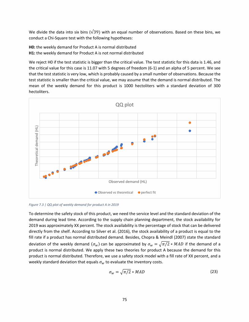
75
We divide the data into six bins (√39) with an equal number of observations. Based on these bins, we
conduct a Chi-Square test with the following hypotheses:
H0: the weekly demand for Product A is normal distributed
H1: the weekly demand for Product A is not normal distributed
We reject H0 if the test statistic is bigger than the critical value. The test statistic for this data is 1.46, and
the critical value for this case is 11.07 with 5 degrees of freedom (6-1) and an alpha of 5 percent. We see
that the test statistic is very low, which is probably caused by a small number of observations. Because the
test statistic is smaller than the critical value, we may assume that the demand is normal distributed. The
mean of the weekly demand for this product is 1000 hectoliters with a standard deviation of 300
hectoliters.
Figure 7.3 | QQ plot of weekly demand for product A in 2019
To determine the safety stock of this product, we need the service level and the standard deviation of the
demand during lead time. According to the supply chain planning department, the stock availability for
2019 was approximately XX percent. The stock availability is the percentage of stock that can be delivered
directly from the shelf. According to Silver et al. (2016), the stock availability of a product is equal to the
fill rate if a product has normal distributed demand. Besides, Chopra & Meindl (2007) state the standard
deviation of the weekly demand (𝜎𝑤) can be approximated by 𝜎𝑤 = √𝜋/2 ∗ 𝑀𝐴𝐷 if the demand of a
product is normal distributed. We apply these two theories for product A because the demand for this
product is normal distributed. Therefore, we use a safety stock model with a fill rate of XX percent, and a
weekly standard deviation that equals 𝜎𝑤 to evaluate the inventory costs.
𝜎𝑤 = √𝜋/2 ∗ 𝑀𝐴𝐷 (23)
Theo
reti
cal d
eman
d (
HL)
Observed demand (HL)
QQ plot
Observed vs theoretical perfect fit

76
The safety stock is calculated by multiplying a safety factor k with the standard deviation of the lead time
demand (𝑠𝑎𝑓𝑒𝑡𝑦 𝑠𝑡𝑜𝑐𝑘 = 𝑘𝜎𝐿). If the safety factor k becomes higher, then we have more safety stock and
fewer shortages, and thus a higher fill rate. The optimal safety factor k for the desired fill rate is determined
with the following formula below (Silver et al., 2016).
𝑓𝑖𝑙𝑙 𝑟𝑎𝑡𝑒 = 1 − 𝐸𝑥𝑝𝑒𝑐𝑡𝑒𝑑 𝑠ℎ𝑜𝑟𝑡𝑎𝑔𝑒 𝑝𝑒𝑟 𝑟𝑒𝑝𝑙𝑒𝑛𝑖𝑠ℎ𝑚𝑒𝑛𝑡 𝑐𝑦𝑐𝑙𝑒
𝐸𝑥𝑝𝑒𝑐𝑡𝑒𝑑 𝑑𝑒𝑚𝑎𝑛𝑑 𝑝𝑒𝑟 𝑟𝑒𝑝𝑙𝑒𝑛𝑖𝑠ℎ𝑚𝑒𝑛𝑡 𝑐𝑦𝑐𝑙𝑒= 1 −
𝐸𝑆𝑃𝑅𝐶
𝑄 (24)
In which the expected shortage per replenishment cycle is equal to 𝜎𝐿𝐺(𝑘), and 𝐺(𝑘) is equal to the
normal-loss function. We use the following assumptions in our model:
1. Fill rate
The stock availability for 2019 was XX percent for all products. Because the demand is normal
distributed, we may assume that the stock availability equals the fill rate (Silver et al., 2016).
Therefore, we assume that the fill rate equals XX percent.
2. Lead time
Grolsch produces five days per week. Product A is produced each day, and therefore we assume
that the lead time equals 1/5 week.
3. Demand per replenishment cycle Q
The mean demand for this product is 1000 hectoliters. Grolsch assumes that this demand is equally
distributed over the week. Because the lead time of this product is 1 day / 0.2 week, we assume
that the demand during the replenishment cycle is 1000 / 5 = 200 hectoliters per day.
4. Hectoliter per pallet
One pallet contains approximately 500 HL
5. Average price per HL
The average price per hectoliter in 2019 was 0.5 euros. Therefore, the value of one pallet is equal
to 0.5 * 500 = 250 euros.
6. Holding costs per pallet
Grolsch assumes that there are no holding costs in the current situation. However, because there
are costs of capital, handling costs, transportation costs, and obsoletes, we assume a holding cost
percentage of 10 percent of the value. Therefore, we assume that the holding costs per pallet are
25 euros.
As can be seen in the formula 23, we need the standard deviation of the lead time demand (𝜎𝐿) instead of
the standard deviation of the weekly demand. Therefore, we multiply the standard deviation of the weekly
demand with the square root of the lead time (𝜎𝐿 = 𝜎𝑤 ∗ √𝐿). We apply Formula 23 and Formula 25 on
the dataset of the current situation, and the dataset with the new forecast from the model. The MAD,
standard deviation of weekly demand, and standard deviation of demand during the lead time are given
for both methods in Table 7.1.
𝜎𝐿 = 𝜎𝑤 ∗ √𝐿 (25)

77
Table 7.1 | MAD and standard deviation of demand for the current forecasting method and Random Forest model
Method MAD
Standard Deviation
Weekly demand (HL) Demand during the lead time (HL)
Current Method 1512
Random Forest 1478 -2,2% -2,2%
The input values for the safety stock calculation are given in Table 7.2
Table 7.2 | Input for calculation
Fill rate XX
Lead time 0.2 Weeks
HL Per pallet 5 hectoliters
Percentage holding costs 10%
Average price per HL (2019) € 50
The average value of pallet € 250
Holding costs per pallet € 25
We can rewrite formula 24 to the formula 26 to calculate G(k). The corresponding safety factor k is found
with the approximation of the normal-loss function and the solver in Excel. The results are given in Table
7.3. We use Formula 26 to determine the value for G(k) in the current situation, which is 0.09497. We find
manually the corresponding safety level k, which is 1.958. Therefore, the safety stock is equal to the safety
factor multiplied with the standard deviation of the lead time demand. The safety stock is 1659 HL or 329
pallets in the current situation. Because we assume that the holding costs per pallet are €90.54, the value
of the safety stock is equal to €29,811 per week and €1,55 million per year. We apply the same calculation
for the dataset with the forecast from the Random Forest. The standard deviation of the demand during
lead time is lower (Table 7.1), which results in lower safety stock. We conclude from Table 7.3 that the
value for the safety stock for the Random Forest model amounts to €29,021 euro safety stock per week,
and 1.51 million euros per year. This means that our model results in a safety stock value decrease of
€41,000 per year. Compared this saving to the total costs of inventory per year, then we conclude that
there is a small improvement. The reason for this is that the forecast accuracy in the current situation is
approximately 85 percent, which is quite high. Therefore, it is difficult to obtain a large improvement.
𝐺(𝑘) =
𝑄(1 − 𝑓𝑖𝑙𝑙 𝑟𝑎𝑡𝑒)
𝜎𝐿
(26)
Table 7.3 | Results safety stock analysis
Situation G(k) k
Safety stock Safety stock costs (euro)
Hectoliter Pallets Per week Per year
Current situation 0.09497 1.958 166 33 823 42,800
Random Forest 0.09714 1.950 162 32 800 41,670
Total 4 1 23 1,134

78
7.4 Conclusion We discussed in Chapter 7 the impact of the model for the demand planning process and the daily
operations. We concluded that the main advantage of this research is the standardization of processes.
The baseline cleaning method is implemented using Excel VBA, and it provides a method of how the
demand planning department obtains a more stable baseline. The model for forecasting promotional
volumes can be used as a decision tool in the demand planning process. The disadvantage of the
promotional forecasting model is that it is a black-box model, so we only know the results and not how it
is derived. The second disadvantage is that the customer support employees do not know the software R.
Therefore, we developed a tool in Excel and a user guide for updating the data in the tool in Appendix G.
We ended this chapter with a review how the forecast accuracy impacts the daily operations for Grolsch.
We analyzed why the forecast accuracy is so important, and how the developed prediction model impacts
the safety stock. The model is tested for one product with high sales and high promotion pressure. From
this analysis, we conclude that the model could lead to a potential saving of 1134 euros per year for this
product.

79
Chapter 8 | Conclusion, Discussion & Recommendations This chapter provides the conclusion (Section 8.1), discussion (Section 8.2) and recommendations (Section
8.3) to the research that was conducted at the demand planning department of Grolsch. This department
observes that the current demand planning process results in a high workload and continuously quick fixes
to meet deadlines and to obtain a good forecast. In the current situation, there is forecasted on the total
demand level, but they desire to distinguish a forecast for baseline demand and promotional demand.
Besides, there is not much standardization in the current process. Therefore, the objective of this research
was:
Developing a standardized method for determining baseline demand based on historical data and to
create a model for forecasting the promotional volume. It should contain well-founded assumptions and
it provides insight into the relations between variables that impact the promotional volume.
8.1 Conclusion We provide first the conclusions for the standardized method that we developed to determine the baseline
sales, after which we conclude the findings for the promotional forecasting model that we developed in
this research.
8.1.1 Method for determining baseline sales We developed a method to determine the baseline demand, and we implemented this method in the
current process using VBA in Microsoft Excel. The method uses historical ex-brewery sales or IRI baseline
sales as input. Based on the promotion pressure and the available IRI data, it selects which data source is
suitable. We clean the sales for promotions, weather, and outliers to obtain a baseline that is
representative of an average year. The sales are cleaned for promotions because promotions are organized
to increase sales. Therefore, they do not belong to the baseline sales. The step for cleaning promotions
takes into account the pre-loading of the promotional volume and the dip in sales after promotion. The
second step in the process is cleaning for the weather. Weather influences the sales of Grolsch, and we
clean therefore the weeks that do not follow a regular weather pattern. The weeks that are influenced by
promotion or weather are replaced with an average of the sales before and after the influenced weeks.
The last step of the method is cleaning for outliers. The sales are cleaned for outliers because it is not
desired that not-recurring events are in the baseline sales. We created for each product-retailer an interval
for low and high season. If the sales of a week are outside this interval, then we replace the sales of that
week with the lower or upper bound of the interval. Nowadays, approximately 20-30 percent of the sales
are sold during a non-promotional period. We analyzed the results of the cleaning method, and we
concluded that the obtained baseline is also around 20-30 percent of the total sales volume. Besides, we
created for each product-retailer a confidence interval to test whether there is a significant difference
between the baseline based on ex-brewery sales or the IRI-baseline. We conclude that there is no
difference in 92 percent of the cases.
8.1.2 Model for forecasting promotional volumes In the second part of the research, we developed a model for predicting promotional volumes. We
concluded from the literature that a baseline-uplift method in combination with linear regression is a
widespread approach for promotional forecasting. However, we found in this research that linear
regression is not applicable for Grolsch promotions, because the input data contains many categorical
variables. Therefore, we investigated the field of machine learning and we concluded that a Random Forest

80
model is most suitable for predicting promotional volumes. The promotional volume for a promotion is
the realized sales minus the baseline sales for that product-retailer. Therefore, we use the baseline that
followed from the baseline cleaning.
We used many variables as input for the prediction model and tested which variables are most important
for predicting the promotional volume. Therefore, we set up different experiments in combination with
feature selection methods. From these experiments, we concluded that the predictors account, product
code, month, price, and promotion mechanism are the most important variables. The disadvantage of a
Random Forest is that it is a black-box model. We have some inputs that result in output, but we cannot
derive how the model comes to this conclusion. We performed 25 experiments to find the input
configuration that results in the lowest cross-validated RMSE. We concluded that the optimal input
parameters for the random forest are mtry = 5 and ntree = 400. Remarkably, the optimal number of
predictors (mtree) equals the total number of predictors. The reason for this is that the predictors account
and product code are very important. If one of these predictors is not included, then the Random Forest
cannot make a good prediction. This shows that there are large differences between promotional volumes
of different product-retailers. At last, we created the final model using the five most important variables,
and the optimal input configuration. We conducted for each promotion category three experiments with
different datasets, to find the dataset that results in the best performance. From these experiments, it can
be concluded that the promotion categories GPP Crate, GPP Can, Summer, Lentebok, and craft-beer have
the best performance if we use only the dataset for that specific promotion category as an input. The other
promotion categories have the best performance if we use a dataset with all categories except for GPP
Promotions as input.
We used 5-fold cross-validation to measure the performance of the forecasting models. The performance
of the current forecasting method and the Random Forest model are presented in Table C1 and Table C2.
We conclude from these tables that the performance of the prediction model is for most promotion
categories better or equal to the current forecasting method. For the promotion categories GPP Can,
Grimbergen, and Kornuit Other, it performs worse for one performance indicator. For the promotion
categories Lentebok and craft-beer, it is not possible to achieve higher performance. The forecasting
model is implemented in an excel tool. We tested the model for a product of GPP Crate, in which we
replaced the current forecast with the forecast from the prediction model. It shows that it leads to a
standard deviation reduction of XX HL per week, with a potential cost saving in safety stock of XX euros
per year.
Table C1 | Performance promotion models for a single promotion category (Current = Current Method, RF = Random Forest Model)
Performance measure
GPP Crate GPP Can Grolsch Summer
Lentebok Craft-beer
Current RF Current RF Current RF Current RF Current RF
MAD 286 257 94 82 52 48 37 40 11 11
MAPE 36% 33% 24% 29% 82% 77% 50% 79% 70% 115%
RMSE 674 603 218 181 107 101 58 63 16 16
wMAPE 19% 17% 31% 27% 96% 41% 37% 39% 55% 54%

81
Table C2 | Performance promotion model for dataset without GPP (Current = Current Method, RF = Random Forest Model)
Performance measure
Grimbergen Kornuit Other Kornuit Crate Low-Promo Herfstbok
Current RF Current RF Current RF Current RF Current RF
MAD (HL) 46 34 46 41 214 158 45 30 91 69
MAPE (%) 64% 70% 61% 67% 68% 50% 41% 37% 87% 68%
RMSE (HL) 96 70 75 63 317 228 89 65 194 137
wMAPE (%) 47% 12% 38% 8% 50% 37% 40% 27% 50% 26%
8.1.3 Practical and scientific contribution This research contributes to the field of promotional forecasting in several ways. The practical contribution
for Grolsch is that they have a method that they can use for determining the baseline sales. This allows
Grolsch to determine the historical promotional volumes. This baseline can be applied for future research
to determine a forecast for the baseline demand. The second practical contribution for Grolsch is that they
have a (decision) tool for forecasting promotional demand.
The scientific contribution is that this research shows a method for determining the baseline sales for a
company in the FMCG industry with a high promotional pressure. The second scientific contribution is that
we show that a widespread approach, the baseline-uplift model with linear regression, is not always
suitable for promotional forecasting with much categorical variables. In this case, it is better to apply
regression tree-based algorithms.
8.2 Discussion In this research, we developed a method for determining the baseline sales from historic data. This
baseline is used as input for the development of the prediction model for promotional volumes. In this
section, we reflect on the research and the created models. First, we discuss the aspects related to the
baseline cleaning, after which we discuss the aspects related to the promotional forecasting model.
8.2.1 Baseline The baseline cleaning methods standardizes and automates the process for determining the baseline sales.
This method cleans historic sales data for promotions, weather, and outliers to determine baseline sales.
A feature that is not included in the cleaning process is the number of stores because were not able to
retrieve this data. However, this data is very relevant because if the number of stores increases, then the
baseline sales will probably increase also. An example is that Retailer G and Retailer H acquired other
retailers in 201X, and therefore the baseline sales will be higher in 201X/201Y. When the baseline is not
corrected for the number of stores, then it is not possible to determine a trend over the baseline because
the sales in one year are higher or lower than other years. Therefore, it would be a nice addition to include
this feature if the data becomes available.
Besides, if we have some weeks impacted by weather or promotions, then we replace the sales of these
weeks with the average sales before and after promotion. This works well for the products that have
regular demand, but it does not result in a good performance for products with intermittent demand or
the products that have sales once every X weeks. An example is when a retailer orders every 5 weeks the
same quantity. Because there are some peaks in the sales data, the method will see these observations as
outliers. These outliers are replaced with zero because the other weeks have no sales. However, the

82
demand planning department should discuss whether these unregular sales have baseline demand
because the sales do not occur regularly.
At last, some retailers only order products during promotion, and they order barely during non-promotion
weeks. They order much during promotion weeks because the products’ price is lower during promotion.
The consequence is forward buying, and that results in lower sales in non-promotion periods. It should be
considered to what extent these products have a baseline because there are only orders during a
promotion. Therefore, the demand planning department hast to decide whether these retailers/products
have baseline sales.
8.2.2 Promotional volume In the second part of the research, we developed a model for forecasting the promotional volume. We
conclude from the results in Table C1 and Table C2 that the models have a better performance or an equal
performance for most promotion categories. However, for the promotion categories Lentebok and craft-
beer, we are not able to obtain a better prediction. A reason could be that the Lentebok promotion is a
seasonal product that is only sold during Q2 and Q3. At the beginning of this period, the product is loaded
in at the retailer. For the craft-beer category, we have a limited number of observations and therefore it
is difficult to make a good prediction. Because the model shows comparable performance to the current
method, it can be used as a decision tool that makes the process more standardized and easier. Besides,
the model was not able to include retailers or brewery information because the promotion pressure is
always high with as a consequence that it is difficult to distinguish the effects of competition. However, it
seems very logical that competition is important. Therefore, the predictions of the model should be
corrected by the customer support employees for forecasting.
Because the price and promotion mechanism are not registered in VisualFabric, we had to retrieve this
data from a database with market data from the revenue management department. The disadvantage of
this database is that it does not contain data for Retailer C, Retailer E, Retailer D & Retailer F. Therefore,
we were not able to include these retailers in the prediction model because we had no data. Besides,
Retailer G has for many products season promotions or year promotions. These promotions are registered
as one promotion, and therefore we had limited data available. Therefore, we were not able to make good
predictions for this category. Therefore, the model does not provide a forecast for Retailer C, Retailer E,
Retailer D, Retailer F, and Retailer G.
We conclude from the interviews with stakeholders and the literature review that the three variables
brand promotion, category promotion, and the number of stores could impact the promotional volume.
However, it is not possible to include these variables in the research because there is no available data for
these variables. A brand promotion is a trend of the last years, and it means that a retailer organizes a
promotion for all products of one brand, such as all Grolsch products. The consequence is that there are
cannibalization effects and that for some products the promotional volume will be lower (Section 3.1).
Another trend is that a retailer offers a promotion on all products within the same category, such as all
crates. When all products within the same category are offered for the same price or promotion
mechanism, then customer loyalty becomes more important as stated in Section 3.1 and Section 3.2. The
last variable that is not included in the research is the number of stores because this variable is not
registered in the system. However, this is a very important variable because retailers open and close
supermarkets, which cause a higher or lower promotional volume.

83
Besides, the model does not work for new products. The Random Forest needs historic data as input to
make a forecast for a promotion. If a new product is introduced, then there is no data or not much data
available with as a consequence that we were not able to make a (good) prediction for these products.
This also applies to promotions that did not occur before in the dataset, because the model has not enough
data in the dataset to make a good prediction. For example, if a promotion mechanism is used that is not
used normally, the model can predict this category, but the quality of the prediction cannot be guaranteed.
In this research, we used machine learning to determine a forecast for the promotional volume. For
machine learning, it is very important that the input data is not influenced by human decisions. However,
the promotional data is not random because it is based on the sales strategies of Grolsch. The strategy of
Grolsch for a product determines the promotional volume and the baseline sales. If there are more (less)
promotions organized, then the baseline sales will be lower (higher). Therefore, the baseline sales and the
promotional sales of a product are not completely random. For machine learning, the input data of all
years must be comparable. This should be considered when the model is updated.
8.3 Recommendations The objective of this research was to develop a method for determining the baseline sales, and a model
for forecasting promotional volumes. Both goals are implemented in an Excel tool, which can be used by
the customer support employees and the demand planning department. In this section, we propose some
recommendations for further research.
8.3.1 Baseline Forecasting We created in this research a method to determine the baseline sales. This method is based on historical
total sales data, and it is cleaned for promotions, weather, and outliers. We used this baseline to calculate
the promotional volume of historical promotions. Another feature of this baseline is that it could be used
for forecasting baseline demand. We described which steps should be taken for forecasting baseline
demand in Section 4.5. First, we need to clean the baseline for events, after which time series analysis
(trend and seasonality patterns) and forecasting techniques can be applied, such as exponential smoothing
or linear trend. This will result in a forecast for the baseline demand.
8.3.2 Number of stores We were not able to include the number of stores in the baseline cleaning method and the promotional
forecasting model because the information was not available. It occurs that retailers open new locations,
or they increase the number of stores by acquiring other retailers. When there are more stores, then there
are more locations to buy a product and the sales will increase. The consequence is that in the following
year, the baseline sales and the promotional volumes will be higher. Therefore, the sales between years
are not comparable, and so it is more difficult to analyze whether there is a trend in the sales. We think
that this variable is important for determining the baseline sale and making a prediction of the promotional
volume. Therefore, it might be useful to investigate the impact of the number of stores on the baseline
and the promotional volume when this data becomes available.
8.3.3 Data collection We spend quite some time to acquire (good) data. We noticed during the process that a lot of promotional
characteristics are not registered in VisualFabric, such as price and promotion mechanism. This
information was lacking in most cases, but sometimes the customer support employees added this
information manually. However, this was not done a standardized way which makes it difficult to retrieve
84
it. Because the database consists of many promotions, we were not able to obtain this data manually. This
would be too time-consuming, and it does not suit in the timeframe of this research.
The predictors product, retailer, and month are registered in VisualFabric but the variables price and
promotion mechanism are not registered in VisualFabric. However, for some retailers, the price and
promotion mechanism are stored in a database with market data retrieved from the revenue management
department. This database has two disadvantages, namely that there is lots of unclean data and that some
retailers are not in the database. Because there is a lot of unclean data, we had to spend a lot of time to
clean it. Besides, the retailers Retailer C, Retailer E and Retailer F are not present in the dataset. This means
that we do not have the prices and promotion mechanisms for these promotions with as consequence
that we cannot forecast the promotional volumes.
If Grolsch wants to base their forecasts on data, then there needs to be data with high quality. Besides, it
was difficult and time-consuming to retrieve the data which does not makes it easy to update the model.
Therefore, we recommend standardizing the way of storing data such that it becomes easier to analyze
the promotional volumes and to update the model. An example could be that the customer support
employees store the price and promotion mechanism of a promotion manually in VisualFabric. Then, all
information is available in the same format and for all retailers/products.
8.3.4 New product forecasting We developed in this research a forecasting model for promotional volumes. This model needs historical
data as input to make a prediction. With New Product Forecasting, in most cases there is no sales data or
not much sales data available. This causes that it could be difficult to obtain a good forecast from this
model. This means that the forecasting model is not able to make a prediction for New Products. We know
from the supply chain planning department that they observe a high obsolete percentage for this type of
products. Therefore, these promotions also need a good forecast. We recommend doing more research in
the field of new product forecasting such that these products also have a good forecast.

85
References Adebanjo, D., & Mann, R. (2000). Forecasting consumer demand 223 Identifying problems in forecasting
consumer demand in the fast moving consumer goods sector. An International Journal (Vol. 7). # MCB University Press. Retrieved from http://www.emerald-library.com
Ali, Ö. G., Sayin, S., van Woensel, T., & Fransoo, J. (2009). SKU demand forecasting in the presence of promotions. Expert Systems with Applications, 36(10), 12340–12348. https://doi.org/10.1016/j.eswa.2009.04.052
Basson, L. M., Kilbourn, P. J., & Walters, J. (2019). Forecast accuracy in demand planning: A fast-moving consumer goods case study. Journal of Transport and Supply Chain Management, 13. https://doi.org/10.4102/jtscm.v13i0.427
Breiman, L. (2001). Randomforest2001. Machine Learning. https://doi.org/10.1017/CBO9781107415324.004
Caglayan, N., Satoglu, S. I., & Kapukaya, E. N. (2020). Sales forecasting by artificial neural networks for the apparel retail chain stores. In Advances in Intelligent Systems and Computing (Vol. 1029, pp. 451–456). Springer Verlag. https://doi.org/10.1007/978-3-030-23756-1_56
Chen, S. F. S., Monroe, K. B., & Lou, Y. C. (1998). The effects of framing price promotion messages on consumers’ perceptions and purchase intentions. Journal of Retailing. https://doi.org/10.1016/S0022-4359(99)80100-6
Chopra, S., & Meindl, P. (2007). Supply Chain Management. Strategy, Planning & Operation. In Das Summa Summarum des Management. https://doi.org/10.1007/978-3-8349-9320-5_22
Cooper, L. G., Baron, P., Levy, W., Swisher, M., & Gogos, P. (1999). PromoCastTM: A new forecasting method for promotion planning. Marketing Science, 18(3), 301–316. https://doi.org/10.1287/mksc.18.3.301
Croxton, K., Lambert, D., Garcia-Dastugue, S., & Rogers, D. (2002). The Demand Management Process. International Journal of Logistics Management, The, 13, 51–66. https://doi.org/10.1108/09574090210806423
Divakar, S., Ratchford, B. T., & Shankar, V. (2005). CHAN4CAST: A multichannel, multiregion sales forecasting model and decision support system for consumer packaged goods. Marketing Science, 24(3), 334–350. https://doi.org/10.1287/mksc.1050.0135
Freo, M. (2005). The impact of sales promotions on store performance: A structural vector autoregressive approach. Statistical Methods and Applications, 14(2), 271–281. https://doi.org/10.1007/s10260-005-0114-x
Gilbert, D. C., & Jackaria, N. (2002). The efficacy of sales promotions in UK supermarkets: A consumer view. International Journal of Retail & Distribution Management, 30(6), 315–322. https://doi.org/10.1108/09590550210429522
Gupta, S. (1988). Impact of Sales Promotions on When, What, and How Much to Buy. Journal of Marketing Research, 25(4), 342. https://doi.org/10.2307/3172945
Hastie, T., Tibshirani, R., James, G., & Witten, D. (2006). An Introduction to Statistical Learning, Springer Texts. Springer Texts. https://doi.org/10.1016/j.peva.2007.06.006
Heerde, Hj Van, & Gupta, S. (2005). The Origin of Demand: A System to Classify the Sources of Own-

86
Demand Effects of Marketing Instruments. Retrieved from http://wms-soros.mngt.waikato.ac.nz/nr/personal/harald van heerde/doc/The Origin of Demand.pdf
Heerkens, H., & Van Winden, A. (2017). Solving Managerial Problems Systematically. Noordhoff Uitgevers.
Huang, T., Fildes, R., & Soopramanien, D. (2014). The value of competitive information in forecasting FMCG retail product sales and the variable selection problem. European Journal of Operational Research, 237(2), 738–748. https://doi.org/10.1016/j.ejor.2014.02.022
Lam, S. Y. S. Y., Vandenbosch, M., Hulland, J., & Pearce, M. (2001). Evaluating promotions in shopping environments: Decomposing sales response into attraction, conversion, and spending effects. Marketing Science, 20(2), 194–215. https://doi.org/10.1287/mksc.20.2.194.10192
Luijten, A. L. J. . (2012). De effectiviteit van sales promoties: Een studie naar de effecten van sales promotie op het huishoudelijk aankoopgedrag in markten van Fast Moving Consumer Goods.
Ma, S., Fildes, R., & Huang, T. (2016). Demand forecasting with high dimensional data: The case of SKU retail sales forecasting with intra- and inter-category promotional information. European Journal of Operational Research, 249(1), 245–257. https://doi.org/10.1016/j.ejor.2015.08.029
Owens, D. L., Hardman, M., & Keillor, B. (2001). The differential impact of price-related consumer promotions on loyal versus non-loyal users of the brand: A field study investigation. Journal of Promotion Management, 6(1–2), 113–131. https://doi.org/10.1300/J057v06n01_10
Peters, J. (2012). Improving the promotional forecasting accuracy for perishable items at Sligro Food Group B.V. BSc Industrial Engineering and Management Science – TU.
Ramanathan, U., & Muyldermans, L. (2010). Identifying demand factors for promotional planning and forecasting: A case of a soft drink company in the UK. International Journal of Production Economics, 128(2), 538–545. https://doi.org/10.1016/J.IJPE.2010.07.007
Silver, E. A., Pyke, D. F., & Thomas, D. J. (2016). Inventory and Production Management in Supply Chains. Inventory and Production Management in Supply Chains. https://doi.org/10.1201/9781315374406
Tsao, Y.-C. (2016). Pricing and ordering under trade promotion, brand competition, and demand uncertainty. Scientia Iranica, 23(5), 2407–2415.
Van Der Poel, M. J. (2010). Improving the promotion forecasting accuracy at Unilever Netherlands.
Van Donselaar, K. H., Peters, J., De Jong, A., & Broekmeulen, R. A. C. M. (2016). Analysis and forecasting of demand during promotions for perishable items. International Journal of Production Economics, 172, 65–75. https://doi.org/10.1016/j.ijpe.2015.10.022
van Heerde, H. J., Leeflang, P. S. H., & Wittink, D. R. (2005). How Promotions Work: SCAN*PRO-Based Evolutionary Model Building. SSRN Electronic Journal, 54, 198–220. https://doi.org/10.2139/ssrn.321003
van Heerde, Harald, Leeflang, P., & Wittink, D. (2002). How promotions work: SCAN⁎PRO-based evolutionary model building. Schmalenbach Business Review, 54, 198–220. https://doi.org/10.2139/ssrn.321003
Zeybek, Ö., Kaya, T., Ülengin, B., & Öztürk, I. (2020). Decomposing the impact of sales promotions on a large scale retailer’s business performance. Advances in Intelligent Systems and Computing (Vol. 1029). https://doi.org/10.1007/978-3-030-23756-1_58

87
Appendices
Appendix A | Confidence interval for the baseline cleaning method We construct a 95 percent confidence interval for the difference in baseline per week based on the ex-
brewery sales and the baseline per week based on the IRI-baseline. We have in total 156 observations (i =
1,2,…,156). We define Xi as the baseline per week based on ex-brewery data, Yi as the baseline per week
based on the IRI-baseline, and Wi as the difference in baseline per week (Xi – Yi). We calculate for all 156
observations Wi. Based on these differences, we construct a 95 percent confidence interval using the
following formulas:
�̅� ± 𝑡𝑛−1,1−𝑎/2√𝑣𝑎𝑟[�̅�]
�̅� = 1
𝑛∑ 𝑊𝑗
𝑛
𝑗=1
𝑉𝑎𝑟[𝑊]̅̅ ̅̅ = 𝑉𝑎𝑟[�̅�]
𝑛
This results in the following values for the product Product B:
�̅�
√[�̅�]
𝑡155,0.975
LB
UB
The difference in the baseline is not significant, because zero is in the interval.

88
Appendix B | All input variables promotional forecasting model Factor Description Type
Price
Original price The original sell price of the product at a retailer Continuous
Promotion price Promotion price of the product at a retailer Continuous
Discount (€) Discount in euro Continuous
Discount in percentage Discount as a percentage of the regular sales price Continuous
Discount compared to previous promotion (€)
The price difference (€) compared to the previous promotion
Continuous
Discount compared to previous promotion (%)
The price difference (%) compared to the previous promotion
Continuous
Promotion
Promotion mechanism Mechanism used for promotion (X voor Y – Single Buy – 2 halen 1 betalen – 4 halen 2 betalen – 2e halve prijs – overige multibuy – 3 halen 2 betalen – 3 + 1 gratis)
Categorical
Place in folder Place of promotion in folder (Front – Mid – Last) Categorical
Duration The number of days that a promotion is organized Integer
Brand promotion If a promotion is a brand promotion (1), if not then (0) Boolean
Category promotion If a promotion is a category promotion (1), if not then (0) Boolean
Number of stores The number of stores in which the promotion is organized Integer
Retailer
Retailer Level of competition if another retailer has the same product in promotion (high, medium or low)
Categorical
Account Retailer at which promotion is organized Categorical
Beer companies
Brewery Level of competition if another brewer has a product in the same category in promotion. These are five levels (A,B,C,D,E) in which A = high and E = none.
Categorical
Period
Mean temperature A category that represents the average temperature of the week in which the promotion is organized.
Categorical
Maximum temperature A category that represents the maximum temperature of the week in which the promotion is organized
Categorical
Number of ADS The average number of ADS days that the week of promotion is organized.
Integer
Event Whether there is a special event during the promotion week.
Categorical
Month The month in which the promotion is organized. Categorical
Product
Product cluster The product cluster to which the SKU belongs Categorical
Product Product code of a product Categorical
Packsize The pack size of the product Categorical
Baseline sales The baseline sales of the product in the promotion week Continuous

89
Appendix C | Results baseline-uplift method / Linear Regression This appendix is removed due to confidential information

90
Appendix D | Results from experimental design for optimal input configuration Random
Forest
mtry ntree RMSE Rsquared MAE
1 200 2264.081 0.370873 1211.607
1 400 2254.763 0.37701 1203.609
1 600 2263.293 0.373013 1211.635
1 800 2255.296 0.378671 1204.596
1 1000 2263.465 0.374049 1211.709
2 200 2020.593 0.435823 1053.487
2 400 2015.863 0.438747 1043.641
2 600 2021.489 0.440594 1050.535
2 800 2022.57 0.434104 1051.402
2 1000 2018.848 0.438635 1046.775
3 200 1895.992 0.476595 959.6793
3 400 1892.666 0.479089 958.8461
3 600 1893.612 0.480522 957.0888
3 800 1885.445 0.485664 952.5144
3 1000 1889.203 0.481158 955.9534
4 200 1799.291 0.523771 897.4359
4 400 1802.794 0.520918 895.5254
4 600 1798.583 0.526082 896.3813
4 800 1793.748 0.527545 893.6363
4 1000 1790.809 0.530801 891.6609
5 200 1682.672 0.592376 831.4668
5 400 1693.829 0.584209 834.3455
5 600 1678.101 0.594482 831.3753
5 800 1695.887 0.582449 838.1097
5 1000 1686.291 0.589051 834.1119

91
Appendix E | Chi-Square test Normal Demand This appendix is removed due to confidential information

92
Appendix F | Results of creating the final forecasting model This appendix shows the results of the experiments conducted in Section 6.5.
GPP Crate
Data input Current GPP Crate GPP All data
MAD 286 257 289 361
MAPE 36% 33% 33% 32%
MSE 454180 363465 450728 658547
RMSE 674 603 671 812
wMAPE 19% 17% 15% 16%
GPP Can
Data input Current GPP Can GPP All data
MAD 94 82 118 93
MAPE 24% 29% 50% 46%
MSE 47670 32725 40807 25953
RMSE 218 181 202 161
wMAPE 31% 27% 3% 18%
Grolsch Summer
Data input Current Grolsch Summer No GPP All data
MAD 52 48 49 49
MAPE 82% 77% 83% 84%
MSE 11531 10218 10670 9430
RMSE 107 101 103 97
wMAPE 96% 41% 81% 37%
Lentebok
Data input Current Lentebok No GPP All data
MAD 37 40 42 43
MAPE 50% 79% 85% 93%
MSE 3407 3973 4019 4305
RMSE 58 63 63 66
wMAPE 37% 39% 0.07 37%

93
Grimbergen
Data input Current Grimbergen No GPP All data
MAD 46 37 34 37
MAPE 64% 60% 70% 76%
MSE 9300 5203 4860 4985
RMSE 96 72 70 71
wMAPE 47% 38% 12% 33%
Kornuit Other
Data input Current Kornuit Other No GPP All data
MAD 46 43 41 42
MAPE 61% 75% 67% 75%
MSE 5671 4805 4004 3977
RMSE 75 69 63 63
wMAPE 38% 35% 0.08 30%
Grolsch Seasonal Product
Data input Current Seasonal Product No GPP All Data
MAD 26 34 27 46
MAPE 59% 189% 166% 199%
MSE 1973 2200 1428 5041
RMSE 44 47 38 71
wMAPE 48% 63% 2% 68%
Herfstbok
Data input Current Herfstbok No GPP All data
MAD 91 71 69 72
MAPE 87% 79% 68% 68%
MSE 37628 19433 18781 24850
RMSE 194 139 137 158
wMAPE 50% 39% 0.26 32%
Low-Promo
Data Input Current Low-Promo No GPP All data
MAD 45 36 30 32
MAPE 41% 38% 37% 35%
MSE 7998 8081 4172 8244
RMSE 89 90 65 91
wMAPE 40% 32% 27% 28%

94
Kornuit Crate
Data Input Current Kornuit Crate No GPP All data
MAD 206 165 158 152
MAPE 67% 70% 50% 51%
MSE 95097 56361 51850 52995
RMSE 308 237 228 230
wMAPE 48% 38% 37% 35%

95
Appendix G | Updating the framework This appendix is removed due to confidential information