Public Health Benefits per kWh of Energy Efficiency and

May 2021 – Second Edition

Public Health Benefits per kWh of Energy Efficiency and Renewable Energy in the United States: A Technical Report

Contents Acknowledgments........................................................................................................................... 1

What’s New for the Benefits-per-Kilowatt-hour Values? .............................................................. 2

Executive Summary ........................................................................................................................ 2

When to use the Benefits-per-kWh values .................................................................................. 2

When not to use the Benefits-per-kWh values ........................................................................... 3

Benefits-per-kWh values ............................................................................................................ 3

Understand the Values ................................................................................................................ 3

Introduction ..................................................................................................................................... 6

Background ..................................................................................................................................... 7

Methods........................................................................................................................................... 9

Overview of Approach .............................................................................................................. 10

Modeling Scenarios Development ............................................................................................ 11

Project, Program, and Policy Size Assumptions ....................................................................... 14

Electricity and Emissions Modeling ......................................................................................... 16

Air Quality and Health Impact Modeling ................................................................................. 16

Developing the Benefits-per-kWh Estimates ............................................................................ 18

Uncertainty ................................................................................................................................ 19

Limitations ................................................................................................................................ 22

Results ........................................................................................................................................... 24

Discussion ..................................................................................................................................... 30

Conclusions ................................................................................................................................... 31

References ..................................................................................................................................... 31

Appendix A: AVoided Emissions and geneRation Tool (AVERT) ............................................. 36

Appendix B: Co-Benefits Risk Assessment (COBRA) Health Impacts Screening and Mapping

Tool ............................................................................................................................................... 38

Appendix C: Sensitivity Analyses on Project, Program, or Policy Size and Peak Energy-

Efficiency Definition .................................................................................................................... 41

Appendix D: Top 200 Hours of Demand Benefit-per-kWh Results............................................. 50

Appendix E: Health Impact Functions .......................................................................................... 51

Appendix F: Health Benefits Valuation ........................................................................................ 53

Appendix G: Detailed Benefits-per-kWh Results ......................................................................... 54

Appendix H: Comparison Between 2017 and 2019 BPK Values ................................................. 61

Appendix I: Conversions .............................................................................................................. 63

1

Acknowledgments This report was developed by the U.S. Environmental Protection Agency (EPA) State and Local

Climate and Energy Program within the Climate Protection Partnerships Division of EPA’s

Office of Atmospheric Programs. Emma Zinsmeister led a technical team of EPA experts to

develop this report, including Colby Tucker, David Tancabel, Neal Fann, and Elizabeth Chan,

with significant analytic support from David Cooley and Kait Siegel of Abt Associates. Carolyn

Snyder, Director of EPA’s Climate Protection Partnerships Division, and Maggie Molina, Chief

of EPA’s State and Local Branch, provided leadership and management support for the project.

The EPA team would like to thank the following technical experts for comments they provided

on earlier drafts of this report (with affiliations from the time of their review): Susan Annenberg

(George Washington University), James Critchfield (EPA), Tom Eckman (Lawrence Berkeley

National Laboratory), Mimi Goldberg (DNV GL), Etan Gumerman (Nicholas Institute, Duke

University), Sara Hayes (American Council for an Energy-Efficient Economy), Ed Holt (Ed Holt

and Associates), David Hoppock (Maryland Public Service Commission), Jeff Loiter (Optimal

Energy), Dev Millstein (Lawrence Berkeley National Laboratory), Nancy Seidman (Regulatory

Assistance Project), Jason West (University of North Carolina), and Ryan Wiser (Lawrence

Berkeley National Laboratory).

EPA would also like to thank Pat Knight and Caitlin Odom from Synapse Energy Economics

Inc. for their assistance with AVoided Emissions and geneRation Tool (AVERT) for this

analysis.

2

Executive Summary EPA has developed a set of values that help state and local government policymakers and other

stakeholders estimate the monetized public health benefits of investments in energy efficiency

and renewable energy (EE/RE) using methods consistent with those EPA used for health benefits

analyses at the federal level. These values estimate the potential public health benefits of avoided

emissions of fine particulate matter (PM2.5) and other precursor pollutants.

EPA continually reviews methods and assumptions for quantifying public health benefits. The

values presented here and the associated documentation have been updated to reflect data from

the electricity sector for 2019. These values will continue to be updated as appropriate to reflect

future data, as well as any changes in methods or assumptions.

When to use the Benefits-per-kWh values Health Benefits-per-Kilowatt-hour (BPK) values are reasonable approximations of the health

benefits associated with EE/RE investments due to estimated reductions of PM2.5 and other

precursor pollutants. These values can be used for preliminary analysis when comparing across

state and local policy scenarios to indicate direction and relative magnitude. Examples of

analyses where it would be appropriate to use them include:

• Estimating the public health benefits of regional, state, or local-level investments in

EE/RE projects, programs, and policies

• Understanding the cost-effectiveness of regional, state, or local-level EE/RE projects,

programs, and policies

• Incorporating health benefits in short-term regional, state, or local policy analyses and

decision-making

What’s New for the Benefits-per-Kilowatt-hour Values? EPA has updated the 2017 Benefits-per-Kilowatt-hour (BPK) values with 2019 data. In addition to

updating the data used to calculate the BPK values, EPA has added new features and updated the

methodology, including:

• Revised regions. The BPK values are now calculated for the 14 revised regions in AVERT

v3.0, rather than the 10 regions from AVERT v2.3. See more about the AVERT regions in

the Electricity and Emissions Modeling section on page 16.

• Additional technology types. EPA developed BPK values for two new technology types,

including offshore wind and distributed (rooftop) solar. See more about the technology

types for the BPK values in the Modeling Scenarios Development section on page 11.

• Avoided transmission and distribution losses in values related to energy efficiency. EPA

made it easier for users evaluating energy efficiency scenarios by incorporating avoided

power sector T&D losses for energy efficiency technologies. See more about this change in

the Developing the Benefits-per-kWh Estimates section on page 18.

3

When not to use the Benefits-per-kWh values BPK values are not a substitute for sophisticated analysis and should not be used to justify or

inform federal regulatory decisions. They are based on data inputs, assumptions, and methods

that approximate the dynamics of energy, environment, and health interactions and include

uncertainties and limitations, as documented in this technical report.

Benefits-per-kWh values EPA used a peer reviewed methodology and tools to develop a set of screening-level regional

estimates of the annual dollar benefits per kilowatt-hour from six different types of EE/RE

initiatives.

• Uniform Energy Efficiency – Energy efficiency projects, programs, and policies that

achieve a constant level of savings over one year,

• Energy Efficiency at Peak – Energy efficiency projects, programs, and policies that

achieve savings during 12pm-6pm when energy demand is high (i.e., peak hours),

• Distributed Solar Energy – Projects, programs, and policies that increase the supply of

distributed solar energy available (e.g., rooftop solar generation),

• Utility Solar Energy – Projects, programs, and policies that increase the supply of

energy available from utility-scale solar,

• Onshore Wind Energy – Projects, programs, and policies that increase the supply of

onshore wind available (e.g., wind turbines), and

• Offshore Wind Energy – Projects, programs, and policies that increase the supply of

offshore wind available (e.g., wind turbines).

Understand the Values EPA created BPK values using existing

tools, including EPA’s AVoided

Emissions and geneRation Tool

(AVERT) and CO-Benefits Risk

Assessment (COBRA) Health Impacts

Screening and Mapping Tool. BPK

values are:

• Available for each of the six

project types for each of the 14

AVERT regions

• Based on 2019 electricity

generation data and emissions, population, baseline mortality incidence rate, and income

growth projections

• Presented in 2019 dollars and reflecting the use of either a 3% or a 7% discount rate as

recommended by EPA’s Guidelines for Preparing Economic Analyses (2010)

• Calculated using the same health impact functions EPA uses for regulatory impact

analyses, including the calculation of low and high estimates of mortality. The low and

high estimates of mortality are derived using two different health impact functions that

have differing assumptions regarding human sensitivity to changes in PM2.5 levels.

Figure ES-1. AVERT Regions.

4

With BPK, states and communities can easily estimate the annual dollar value of the outdoor air

quality-related health impacts of EE/RE scenarios occurring within a five-year time horizon.

Users can evaluate many EE/RE scenarios by multiplying the BPK values (Table ES-1) by the

number of kWh saved from EE or generated from RE. Users are encouraged to review the

caveats described within this technical report to ensure these values are appropriate for their use.

This report also describes the uncertainties associated with modeled estimates, which users

should keep in mind when interpreting or reporting results.

5

Table ES-1. 2019 Benefits-per-kWh Values (cents per kWh, 2019 USD, 3% discount rate*)

Region Project Type

3% Discount Rate

2019 ¢/kWh

(low)

2019 ¢/kWh

(high)

California

Uniform EE 0.67 1.51

EE at Peak 0.74 1.67

Utility Solar 0.65 1.47

Distributed Solar 0.64 1.44

Onshore Wind 0.63 1.41

Offshore Wind 0.67 1.50

Carolinas







Central






Florida






Mid-

Atlantic







Midwest






New

England







Region Project Type

3% Discount Rate

2019 ¢/kWh

(low)

2019 ¢/kWh

(high)

New York







Northwest







Rocky

Mountains






Southeast






Southwest






Tennessee






Texas






*BPK values for a 7% discount rate can be found in Table 3,

Results section (p. 28).

6

Introduction State and local government policymakers have increasingly been asking for the

U.S. Environmental Protection Agency’s (EPA’s) help in understanding the opportunities for

using energy efficiency and renewable energy (EE/RE) to reduce air pollution and improve

public health. Many recognize that EE/RE projects, programs, and policies can reduce air

pollution emissions from the electric power sector either by decreasing demand for electricity

generation or by displacing fossil fuel-based generation with zero-emitting sources of generation.

They also recognize that these avoided emissions of fine particulate matter (PM2.5) and other

precursor pollutants may lead to tangible public health benefits, such as reducing the number of

premature deaths, incidences of respiratory and cardiovascular illnesses, and missed work and

school days.1 However, in many cases, state and local decision-makers are not quantifying or

fully accounting for the health benefits of existing or planned EE/RE projects, programs, and

policies in their decision-making processes. EPA has found that state and local decision-makers

may not be fully aware of or confident in the available quantification tools and methods; or they

lack the time, resources, or expertise needed to quantify the health benefits.

EPA seeks to address this gap by providing state and local governments and their stakeholders

with tools and information to estimate the public health benefits of EE/RE. In particular, EPA

has developed screening-level regional estimates of the benefits per kilowatt-hour (kWh) of

EE/RE projects, programs, and policies.2 The goal of these estimates is to create credible and

comparable values (i.e., factors) that stakeholders, such as state and local governments, EE/RE

project developers, and nongovernmental organizations (NGOs), can use to estimate health

benefits of EE/RE projects, programs, and policies. EPA has also sought to ensure that these

values are easy to use, and do not require state and local governments or other users to download

specific modeling software packages.

EPA previously released health benefits-per-kilowatt-hour (BPK) values with 2017 data that

represent screening-level estimates of the benefits from fossil fuel-based generation reduced or

avoided as a result of EE, solar, and wind projects, programs, and policies. This report describes

EPA’s approach for updating those values with 2019 data. The estimates use a 2019 profile of

the electricity system to represent the benefits in the near term of EE/RE projects, programs, and

policies that have already been or are about to be implemented. The resulting health BPK values

can be used by a wide range of state and local governments, EE/RE project developers, and other

stakeholders to develop a more complete picture of the public health benefits of existing or

proposed EE/RE projects, programs, and policies. Note that because BPK values provide a

screening-level estimate of health benefits of EE/RE, they may not be appropriate for certain

analyses, such as federal air quality rulemaking.

1 The Health Effects Institute (2018) estimates that in 2016, 105,669 premature deaths in the United States were

attributable to air pollution [93,376 due to PM2.5 and 12,293 due to ozone (O3)].

2 These estimates include the contiguous United States, but do not include Alaska and Hawaii. These states are not

included in the AVoided Emissions and geneRation Tool (AVERT) used to estimate impacts of EE/RE on air

pollution emissions because they do not report emissions data for most of their electric generating units (EGUs) to

EPA. Alaska and Hawaii are also not included in the CO-Benefits Risk Assessment (COBRA) Health Impacts

Screening and Mapping Tool used to estimate the health impacts of EE/RE because they were not included in the air

quality modeling originally used to develop the tool.

7

Background Electricity generation in the United States is essential to our economy but it also results in

significant emissions of air pollution, depending upon how it is generated. In 2017, the electricity

generation sector emitted more than 1 million tons each of nitrogen oxides (NOx) and sulfur

dioxide (SO2); and more than 100,000 tons of PM2.5, which is roughly equivalent to the PM2.5

emissions of highway vehicles in that year (EPA 2020a). Emissions of these pollutants can result

in serious health impacts, including premature mortality, non-fatal heart attacks, asthma

exacerbations, and other respiratory diseases. EPA’s retrospective analysis of the Clean Air Act

(CAA) found that approximately 85% of the public health benefits of air quality regulations are

due to PM reductions, with the remainder coming from other air pollutants, such as ozone (O3)

(EPA 2011).

While the U.S. electric power sector has historically been a significant source of air pollution, the

sector has undergone rapid change in recent years. Between 2007 and 2018, coal and oil

generation sources combined have decreased from just over 50% of the U.S. generation resource

mix to 27.5%; and renewables, including wind, solar, and geothermal, have increased from just

over 1% to nearly 9% of the resource mix (Figure 1). Similarly, electricity savings from energy-

efficiency programs were over 180 terawatt-hours (TWh) in 2016, an increase of more than

115% from 2008 (IEI 2017). These changes amount to a cleaner U.S. electric power sector with

reduced emissions and health impacts.

Figure 1. U.S. Generation Resource Mix, 2007–2018.

Source: EPA eGRID.

In order to help state and local governments quantify the health benefits of EE/RE, EPA first

needed to understand the current state of the scientific literature to determine if there are best

practices or factors that states could apply. EPA commissioned a literature review that examined

0% 10% 20% 30% 40% 50% 60% 70% 80% 90% 100%

2018

2016

2014

2012

2009

2007

Coal Oil Gas Nuclear Hydro Biomass Wind Solar Other

8

more than 60 studies for BPK values in order to better understand current methods and health

benefits of EE/RE projects, programs, and policies (EPA 2017). Through the literature review,

EPA found that the results varied depending on the approach used, the benefits included, and the

geographic focus of the analysis. Therefore, the resulting sets of BPK values identified in the

literature review were not easily comparable to one another.

Lawrence Berkley National Laboratory (LBL), for example, published several studies examining

both the prospective and retrospective health benefits from wind, solar, and renewable portfolio

standard (RPS) programs across the United States (Table 1). The benefits reported by each study

are an average value of health benefits calculated using multiple different air quality and health

impact models, including the Air Pollution Emission Experiments and Policy Analysis Model

(AP2), EPA’s benefit-per-ton methodology, EPA’s CO-Benefits Risk Assessment (COBRA)

Health Impacts Screening and Mapping Tool, and the Estimating Air Pollution Social Impact

Using Regression (EASIUR) model. Overall, these studies provide a range nationally between

2.6¢/kWh and 10.1¢/kWh for recent years, and between 0.4¢/kWh and 8.2¢/kWh when looking

prospectively. Other studies included in the literature review generated a different range of

results that were not directly comparable to the LBL estimates, typically because they used a

variety of models or included additional benefits. For example, some of the models used in

studies identified in the literature review include non-health, welfare benefits, such as avoiding

damages from decreased timber and agricultural yields, reduced visibility, accelerated

depreciation of materials, and reductions in recreation services; results from these studies may be

higher than the values calculated using models that focus solely on health benefits.

Table 1. Public Health Benefits from wind, solar, and RPS program across the United States

Program Evaluated Benefit-per-kWh (¢/kWh) Source

2013 RPS programs 2.6¢/kWh– 10.1¢/kWh Barbose et al. 2016

2015 Wind energy 7.3¢/kWh Millstein et al. 2017

2015 Solar energy 4¢/kWh Millstein et al. 2017

2015–2050 RPS Programs 2.7¢/kWh – 8.2¢/kWh Mai et al. 2016

2050 Wind energy 0.4¢/kWh – 2.2¢/kWh Wiser et al. 2016a

2050 Solar energy 0.7¢/kWh – 2.6¢/kWh Wiser et al. 2016b

The literature review also identified two key gaps across all available estimates. While several

studies estimated the benefits per kWh in specific regions, particularly the Northeast and

California, there is no comprehensive set of monetized health benefits per kWh from EE/RE for

all U.S. regions. It is not appropriate to apply the national numbers provided by LBL for specific

regions, because this would not accurately represent the differences in the specific composition

of electricity generation throughout the United States and therefore would not account for

regional differences in emissions. Additionally, the values from the literature are not

methodologically consistent, and can therefore not be compared with confidence. These gaps

limit practitioners’ abilities to include health benefits in the assessments of EE/RE projects or

programs, or policy costs and benefits.

This study fills these gaps identified in the literature review by quantifying and presenting easy-

to-use health benefits values for a range of EE/RE types that are comparable and cover all

regions in the United States. These BPK values are calculated in a similar fashion to EPA’s

existing estimates of monetized public health benefits-per-ton (BPT) of emissions reductions in

9

that both the BPT and BPK estimates take health benefits and divide them by an amount of

emissions or generation reduction (Fann et al. 2009).3

In general, the literature review examined common approaches to estimating BPK values and

identified a series of best practices for estimating these values in the United States. The best

practices include:

1. Establish a set of public health BPK values for interventions in specific regions, rather

than a single national value, to account for regional differences in generation and air

pollution control technologies.

2. Establish separate BPK values for different types of EE/RE projects, programs, and

policies, such as wind, solar, uniform EE, and EE at peak, to account for how different

technologies impact the load (i.e., demand) curve.4

3. Establish BPK values for interventions of varying capacity to capture the benefits

stemming from EE/RE interventions that can displace power from baseload, intermediate

load, and peaking units.

4. Account for changes in primary and secondary PM2.5 emissions and, whenever feasible,

changes in O3 concentrations in health BPK values, to capture the majority of health

impacts from outdoor air pollution.5

5. Use emissions, population, and income datasets from the same year to maintain internal

consistency.

The BPK values included in this report are estimated using a method informed by these best

practices. EPA also sought input on the methods for this analysis from outside experts in energy

modeling, health benefits estimation, electricity system operations, and EE/RE policy and

deployment. The remainder of this report describes the methods used to estimate screening-level

BPK values and results of the analysis. This report also contains technical appendices with more

information on the tools and models used in the analysis, as well as the results of sensitivity

analyses performed to address uncertainty in the estimates.

Methods In this section, EPA provides a general overview of the approach used to estimate the near-term

benefits per kWh of EE/RE,6 and then discusses in more detail the electricity, emissions, and

health impact modeling steps used to develop the BPK values.

3 EPA has used the benefits-per-ton (BPT) estimates in multiple regulatory impact assessments for air quality

regulations, such as the Mercury and Air Toxics Standards; the New Source Performance Standards for Petroleum

Refineries; and the National Emission Standards for Hazardous Air Pollutants for Industrial, Commercial, and

Institutional Boilers and Process Heaters. For more information, see https://www.epa.gov/economic-and-cost-

analysis-air-pollution-regulations/regulatory-impact-analyses-air-pollution.

4 See the Energy-Efficiency Scenarios section on page 7 of this report for definitions of uniform EE and EE at peak.

5 EPA’s retrospective analysis of the CAA found that approximately 85 percent of the public health benefits of air

quality regulations are due to PM reductions, rather than O3 (EPA 2011b).

6 The “near term” is defined as approximately the next five years, which is discussed in more detail in the

Limitations section on page 17.

https://www.epa.gov/economic-and-cost-analysis-air-pollution-regulations/regulatory-impact-analyses-air-pollution


10

Overview of Approach

EPA’s approach for estimating the screening-level health benefits per kWh of EE/RE projects,

programs, and policies involves a six-step process:

1. Estimate annual changes in fossil fuel-based electricity generation due to representative

EE/RE projects, programs, and policies.

2. Estimate annual changes in air pollution emissions (NOx, SO2, and PM2.5) due to changes

in fossil fuel-based generation.

3. Estimate annual changes in ambient concentrations of air pollution due to changes in

emissions of primary PM2.5 and precursors of secondary PM2.5.7

4. Estimate annual changes in public health impacts due to changes in ambient

concentrations of PM2.5.

5. Estimate the monetary value of changes in public health impacts.

6. Divide the monetized public health benefits by the change in generation to determine the

health benefits per kWh in 2019 (¢/kWh).

This approach follows well-established methodologies for estimating the magnitude and

economic value of public health benefits of air pollution emissions reductions, which have been

documented in the literature (e.g., Dockins et al. 2004, Fann et al. 2012) and used in recent EPA

Regulatory Impact Analyses (RIAs). Based on these established methodologies, EPA did not

include reductions of carbon dioxide (CO2) in this analysis because those reductions are

generally only included in studies that assess climate and welfare impacts in addition to public

health impacts.

In order to quantify public health benefits in the near term, EPA developed a set of values for the

year 2019. To carry out the approach for these estimates, EPA used two peer-reviewed Agency

tools, the AVoided Emissions and geneRation Tool (AVERT, version 3.0)8 and the COBRA tool

(version 4.0).9 Figure 2 depicts the approach outlined above as it relates to the tools used in this

analysis. These tools are described further in Appendix A: AVoided Emissions and geneRation Tool

(AVERT) and Appendix B: Co-Benefits Risk Assessment (COBRA) Health Impacts Screening and

Mapping Tool.

7 Primary PM2.5 refers to the direct emissions of PM from EGUs. Secondary PM2.5 is created as emissions of SO2 and

NOx [and other pollutants such as ammonia and volatile organic compounds (VOCs)] undergo chemical reactions in

the atmosphere.

8 EPA AVERT; see https://www.epa.gov/statelocalenergy/avoided-emissions-and-generation-tool-avert.

9 EPA COBRA Health Impacts Screening and Mapping Tool; see https://www.epa.gov/statelocalenergy/co-benefits-

risk-assessment-cobra-screening-model.

https://www.epa.gov/statelocalenergy/avoided-emissions-and-generation-tool-avert

https://www.epa.gov/statelocalenergy/co-benefits-risk-assessment-cobra-screening-model

https://www.epa.gov/statelocalenergy/co-benefits-risk-assessment-cobra-screening-model

11

Figure 2. BPK Approach.

Modeling Scenarios Development EPA considered multiple scenarios to estimate changes in electricity generation and emissions

due to EE/RE projects, programs, and policies. During the scenario development process, EPA

sought input from technical experts in EE/RE modeling and analysis, and refined the scenarios

based on their comments. For a description of how these scenarios were used to estimate changes

in electricity generation and emissions, see the

Electricity and Emissions Modeling section on page 16, as well as Appendix A: AVoided

Emissions and geneRation Tool (AVERT).

Renewable Energy Scenarios For RE, EPA modeled separate scenarios for four technology types: onshore wind, offshore

wind, utility solar, and distributed solar. These projects have different impacts on the timing of

generation (i.e., solar only generates during the daytime while wind can generate during more

hours of the day) and may therefore have different impacts on emissions reductions in each

region. EPA modeled each technology in AVERT as 100-megawatt (MW) projects. The

assumptions EPA made in choosing this project size are discussed in more detail in the Project,

Program, and Policy Size Assumptions section (page 14).

Stakeholders can use the individual BPK values to evaluate the benefits of a mix of wind and

solar generation in a particular region. The impacts of EE/RE projects, programs, and policies

are additive, but EPA recommends that the BPK values not be used to estimate benefits of

projects, programs, or policies that exceed 15% of fossil fuel generation in any given hour in a

region. This suggested limit on capacity is set by EPA, due to the fact that AVERT is a historical

dispatch model that is limited in its ability to estimate emissions reductions for projects,

programs, or policies that may significantly alter the generation mix in a region. Capacity added

beyond this 15% cap may have a different impact on emissions that is not captured by the model.

For more information on project size limits when using AVERT, see the Project, Program, and

Policy Size Assumptions (page 14).

•100 MW of wind

•100 MW of solar

•500 GWh of uniform EE

•200 GWh of EE at peak hours (12 p.m. to 6 p.m.)

Scenarios

•Estimate changes in electricity generation using AVERT 3.0

•Estimate changes in emissions of NOX, SO2, and primary PM2.5

AVERT •Estimate air quality changes (primary and secondary PM2.5)

•Estimate monetized public health benefits of changes using COBRA 4.0 and custom 2019 input datasets

COBRA

•Aggregate health benefits for each EE/RE scenario

•Divide health benefits by total electricity displaced

•Inflate results to 2019$

BPK Factors

12

EPA made one change to the approach for calculating the 2019 BPK values compared to the

method for the 2017 values. The 2017 BPK values divide the monetized benefits by the

displaced electricity consumption at the site of the end user, accounting for transmission and

distribution (T&D) losses. The 2019 BPK values use the actual generation from EE/RE sources,

and do not account for T&D losses. The actual generation is an input into AVERT, rather than

the displaced consumption at the site of the end user, which is an output of AVERT. BPK values

are intended to be multiplied by a project’s actual generation. Therefore, the denominator of the

BPK value calculation should be based on actual generation rather than displaced generation at

the site of the end user. This change only affects benefits of the EE and distributed solar

technology types, and it will allow stakeholders to estimate the health benefits of their EE/RE

projects and policies more accurately.

Energy-Efficiency Scenarios EPA developed two scenarios for EE projects, programs, and policies: uniform EE and EE at

peak. EPA modeled uniform EE in AVERT as a 500-gigawatt-hour (GWh) reduction in

electricity demand, distributed evenly throughout all hours of the year. EPA modeled EE at peak

as a 200-GWh reduction distributed evenly (but exclusively) during the limited hours of 12 p.m.

to 6 p.m. on weekdays throughout the year. The assumptions EPA made in choosing this project,

program, and policy size are discussed in more detail in the Project, Program, and Policy Size

Assumptions section on page 14.

Uniform EE is based on a constant reduction in electricity demand applied evenly to all hours of

the year. This assumes that an EE intervention would reduce demand for electricity to the same

degree during all hours of the day and for all seasons. For example, installing energy-efficient

exit signs (which operate 24 hours a day, seven days a week) will result in constant or uniform

reductions, because the signs lower demand during all hours of the year.

The EE at peak scenario assumes that EE reductions occur only during certain times of the day

when demand is highest (often called “peak hours”). In states with warmer climates this is often

the afternoon hours in the summer, while colder states have peak hours during winter mornings;

some states have both morning and afternoon peak hours, and some have both summer and

winter peaks. Air conditioners are an example of a technology that largely impacts the load curve

during summer peak hours. Air-conditioning (A/C) units often consume more electricity during

peak times when people return home from work or school. Installing an energy-efficient air

conditioner is, therefore, an example of a measure that largely affects generation during peak

hours.

The types of electric generating units (EGUs) that typically operate on the margin during peak

hours often differ from those that operate on the margin at other times of the day.10 Peaking units

are generally natural gas units that can ramp up and down quickly compared to baseload coal,

nuclear, or combined cycle gas units that typically operate 24 hours a day. Because emissions

from these types of power plants can vary significantly, the reduction in emissions will likely

10 EPA defines EGUs on the margin as “the last units expected to be dispatched, which are most likely to be

displaced by energy efficiency or renewable energy.” For more information, see chapter 3 of the EPA report,

Quantifying the Multiple Benefits of Energy Efficiency and Renewable Energy: A Guide for State and Local

Governments: https://www.epa.gov/statelocalenergy/quantifying-multiple-benefits-energy-efficiency-and-

renewable-energy-guide-state

https://www.epa.gov/statelocalenergy/quantifying-multiple-benefits-energy-efficiency-and-renewable-energy-guide-state


13

also vary for different types of EE interventions.11 Note that interventions that result in load

reductions during the peak hours may also result in load reductions during off-peak hours. For

example, an energy-efficient A/C unit will result in decreased demand in all hours in which it is

in use, even though the largest reductions will occur during peak hours. Nevertheless, because

these types of EE interventions result in significant load reductions during peak hours, it is useful

to examine the difference in benefits provided by load reductions during peak hours compared to

those from a more uniform load reduction.

In order to model the EE at peak scenario, it is necessary to select a window of time along the

load curve as representative of system peak. However, there is currently no universally agreed-

upon definition of peak hours. When electric utilities are managing the operations of existing

EGUs, they often define the peak period based on the hour of day. Utilities know that demand

tends to increase in the afternoons in the summer and early mornings/late evenings in the winter

and adjust their operations accordingly. EPA compared various definitions of the peak period to

determine which definition to use for estimating the EE at peak BPK values.

EPA reviewed definitions of peak hours from several utilities in different parts of the country.

The definitions of peak hours differed slightly among the utilities (e.g., some are from 2 p.m. to

6 p.m., some include morning hours, some differ by season). EPA conducted a sensitivity

analysis by modeling the same generation reduction for each utility’s definition of peak,

including seasonal variations. For example, Duke Energy defines the peak period in the winter

from 6 a.m. to 9 a.m. and in the summer from 1 p.m. to 6 p.m.; while Pacific Gas and Electric

(PG&E) defines the peak period only during 1 p.m. to 7 p.m. in the summer, but does not include

a peak period in the winter. The sensitivity analysis involved running scenarios for all AVERT

regions using the definitions of the peak period, discussed in more detail in Appendix C:

Sensitivity Analyses on Project, Program, or Policy Size and Peak Energy-Efficiency Definition.

This analysis found that the differences in the definition of peak hours do not result in large

differences in emissions reductions within each region when modeled in AVERT. Therefore,

EPA chose to use the general definition of 12 p.m. to 6 p.m. on weekdays for peak hours, as this

scenario also generated similar emissions reductions compared to the other definitions in all

regions. The results of the sensitivity analysis on the definition of peak hours are discussed in

more detail in Appendix C: Sensitivity Analyses on Project, Program, or Policy Size and Peak

Energy-Efficiency Definition.

In addition to defining the peak period based on

the hour of day, it can also be defined as the top

hours of demand during the year. Utilities

generally use this approach to determine

whether and when to build new capacity,

because they must ensure they have enough

capacity to meet even the highest days of

demand (e.g., the peak period could be based

on the top 200 hours of demand). In most

11 For example, natural gas single cycle turbines are well-suited to serve peak load because of their quick start-up

capability, but these units generally have higher NOx emissions than natural gas combined cycle plants, which are

more efficient and typically serve intermediate or even baseload demand.

RE/EE Scenarios

• 100 MW of added RE capacity (i.e.,

onshore wind, offshore wind, utility

solar, or distributed solar)

• 500 GWh of uniform EE

• 200 GWh of EE during peak hours

(12 p.m. to 6 p.m., weekdays)

14

regions, these high periods of demand are concentrated in the hottest summer afternoons. By

contrast, defining the peak period as 12 p.m. to 6 p.m. on weekdays includes more than 1,500

hours during the year. EPA conducted a sensitivity analysis to compare these definitions of the

peak period by estimating emissions reductions in all AVERT regions using both a “top 200

hours approach” and an “hour of day approach” to define the peak period. The results of this

sensitivity analysis show large differences in the emissions rate in some regions. The full results

of this sensitivity analysis are discussed in Appendix C: Sensitivity Analyses on Project,

Program, or Policy Size and Peak Energy-Efficiency Definition.

After consultation with energy-sector experts, EPA determined that the hour-of-day approach is

more relevant for this analysis. Only very-specific technological interventions or EE programs or

policies would coincide with just the top 200 hours of demand, and the use of this definition

would, therefore, not accurately capture all the benefits from broader programs or policies.

The two definitions of the peak period described above are used for different purposes by electric

utilities—the hour-of-day approach is used to manage existing capacity and the top-hours-of-

demand approach is used to plan for additional capacity or to target demand reduction. EPA

asserts that most independent developers, nonprofits, and state/local users of these BPK values

will be more interested in capturing the impacts of an EE project, program, or policy on the

existing or projected fleet of EGUs, rather than planning for additional capacity, and therefore

the Agency reports values using the hour-of-day approach as the primary BPK values for EE at

peak in this analysis. However, if a utility is planning to use BPK values to estimate the health

benefits of an EE project, program, or policy to avoid investing in new generation, transmission,

and distribution, then the top-hours-of-demand approach may be more appropriate. BPK values

calculated using a top 200 hours approach are shown in Appendix D: Top 200 Hours of Demand

Benefit-per-kWh Results.

Nevertheless, this definition of the peak period should inform how BPK values are used. If an EE

project, program, or policy results in generation reductions only during the top 200 hours of

demand, then it may have a different emissions profile and, therefore, different health benefits,

than the type of EE at peak modeled here. Analysts have the option of developing their own

custom BPK estimates using AVERT and COBRA if the estimates EPA provides do not fit their

unique circumstances.

Project, Program, and Policy Size Assumptions EPA evaluated whether the size of the EE/RE intervention had a meaningful impact on which

EGUs were displaced and tested the linearity of the relationship between avoided kWh and

health benefits. To determine whether the project size would have a large effect on BPK

estimates, EPA conducted a sensitivity analysis by running AVERT with five different project

sizes, ranging from 100 MW to 2,000 MW for RE and 100 GWh to 2,000 GWh for EE. The

results from each AVERT run were entered into COBRA to estimate the health benefits. The

results from both AVERT and COBRA demonstrated strong linear relationships (R2 = 0.9996–

1.0). This means that the BPK values were nearly constant across all the project sizes tested in

the sensitivity analysis. As a result, the results presented here used a single assumption about

project size for each technology type. EPA modeled the RE projects assuming a program,

project, or policy size of 100 MW and modeled the EE projects assuming generation reductions

of 500 GWh for uniform EE scenarios and 200 GWh for EE during peak hours. The full results

15

for this sensitivity analysis are shown in Appendix C: Sensitivity Analyses on Project, Program,

or Policy Size and Peak Energy-Efficiency Definition.

EPA chose the 100 MW and 200 and 500 GWh sizes for RE and EE projects, programs, and

policies respectively because they are large enough to generate significant emissions reductions

but small enough that they do not displace more than 15% of fossil fuel generation in any given

hour and in any region. AVERT is a historical dispatch model that is limited in its ability to

estimate emissions reductions for projects, programs, or policies that may significantly alter the

generation mix in a region. EPA recommends that users avoid modeling scenarios in which the

EE/RE project, program, or policy would reduce more than 15% of fossil-fuel generation in any

given hour.12 The size an individual project, program, or policy can range widely before hitting

that limit, depending on the amount of fossil fuel generation in each region. For example, in the

California region, a 300-MW utility solar project would exceed that limit. In the Midwest,

however, a utility solar project could be as large as 8,000 MW before hitting the 15% threshold.

Table 2 lists the 15% thresholds in all regions for the scenarios included in this report.

Furthermore, EPA also recommends users avoid estimating emissions reductions for projects less

than roughly 1 MW because the resulting emissions reductions estimated by the model are too

small to be distinguished from the underlying variation in the baseline data.

Table 2. AVERT 15% Threshold of Fossil Fuel Generation in 2019

Region

Onshore

Wind

(MW)

Offshore

Wind

(MW)

Utility Solar

(MW)

Distributed

Solar

(MW)

Uniform EE

(GWh)

EE at Peak

(GWh)

California 531 504 289 266 1,882 482

Carolinas 2,063 1,750 827 823 5,726 1,432

Central 1,426 NA 1,532 1,465 7,497 2,569

Florida 3,539 NA 2,538 2,286 10,808 4,319

Mid-Atlantic 5,973 6,583 6,486 6,100 30,207 9,491

Midwest 6,686 NA 7,857 7,497 36,781 11,583

New England 500 311 399 371 1,181 705

New York 629 651 604 562 2,416 896

Northwest 1,341 2,225 636 600 4,299 1,073

Rocky Mountains 769 NA 673 618 4,182 1,150

Southeast 4,049 NA 2,220 2,181 12,096 3,445

Southwest 1,007 NA 759 688 5,805 1,452

Tennessee 1,105 NA 633 620 2,951 843

Texas 2,013 NA 2,664 2,593 13,378 4,590

12 In general, EE/RE impacts greater than 15 percent of regional fossil fuel-load could influence the historical

dispatch patterns that AVERT’s statistical module is based upon. AVERT should not be used to change dispatch

based on future economic or regulatory conditions, such as expected fuel prices, emissions prices, or specific

emissions limits.

16

Electricity and Emissions Modeling To estimate the changes in electricity generation and associated changes in emissions due to

EE/RE projects, programs, and policies (steps 1 and 2 in the overall approach), EPA used

AVERT v3.0. AVERT uses hourly emissions and generation data reported to EPA by EGUs to

determine the air pollution emissions per kWh from each generating unit, as well as the

probability that a given unit will be operating during a given hour.13 AVERT uses this

information to estimate which fossil fuel-fired units will likely be affected by EE/RE projects,

programs, and policies; and the amount of emissions displaced or avoided. The results from

AVERT are the estimated emissions reductions of NOx, SO2, and PM2.5 from the modeled EE or

RE project, program, or policy. The results from AVERT are presented at the county, state, and

regional levels.

The 2019 estimates in this

analysis were developed using

actual emissions and

generation of fossil fuel-fired

EGUs in 2019, which are built

into the latest version of

AVERT. The assumptions

about how AVERT uses

historical data to estimate

emissions reductions are

discussed in more detail in

Appendix A: AVoided

Emissions and geneRation

Tool (AVERT).

EPA developed separate

estimates for each of the 14

AVERT regions (Figure 3) in order to account for regional differences in generation power plant

fuel mixes and air pollution control technologies.14 These regions are based on aggregations of

one or more balancing authorities. EPA modeled each scenario, outlined above, in each region in

2019; 76 estimates of emissions reductions were developed.

Air Quality and Health Impact Modeling Once EPA developed estimates of emissions reductions by applying AVERT for all scenarios,

EPA used the COBRA Health Impacts Screening and Mapping Tool (v4.0) to complete steps 3,

4, and 5 of the approach—estimating changes in ambient air quality, impacts on public health,

and monetized health benefits from emissions reductions, respectively.

COBRA uses a reduced-form air quality model called the Phase II Source-Receptor (S-R) Matrix

to develop screening-level estimates of how changes in emissions at source counties will affect

13 Facilities are required under 40 CFR Part 75 to report information on emissions, heat rate, and generation to

EPA’s Clean Air Market Division (CAMD) for EGUs 25 MW or larger. 14 Note that AVERT implicitly accounts for control technologies because it uses unit-level emissions data to

estimate emissions from electricity generation.

Figure 3. AVERT Regions.

17

ambient PM2.5 concentrations in receptor counties. The S-R Matrix was developed using multiple

runs from the Climatological Regional Dispersion Model (CRDM), a more sophisticated air

quality model, and it is intended as a screening-level tool, which can be run more quickly than

the full model. COBRA accounts for both primary (i.e., directly emitted) PM2.5 emissions and the

formation of secondary PM2.5 in the atmosphere from the reaction of SO2 and NOx with

ammonia (NH3).

COBRA also uses concentration-response (C-R) functions from the epidemiological literature to

determine how changes in ambient PM2.5 concentrations will impact health outcomes, such as

premature mortality, non-fatal heart attacks, asthma exacerbations, and other respiratory

symptoms. Finally, COBRA uses established valuation functions from the economic literature to

estimate the monetary value of each health outcome. C-R and valuation functions used in

COBRA are consistent with those used in EPA’s Environmental Benefits Mapping and Analysis

Program (BenMAP) and in RIAs conducted by the Agency. COBRA assumes that National

Ambient Air Quality Standards (NAAQS) are met in all states and counties, and, therefore,

estimates incremental health benefits from reduced exposure below the standards.15 The result

from COBRA is the estimated avoided public health outcomes from emissions reductions and

the monetary value of those avoided public health outcomes. The results from COBRA are

presented at the county level. For more information on the COBRA tool, see Appendix B: Co-

Benefits Risk Assessment (COBRA) Health Impacts Screening and Mapping Tool; for detailed

information on the C-R functions used in COBRA, see Appendix E: Health Impact Functions;

and for detailed information on the valuation functions used in COBRA, see Appendix F: Health

Benefits Valuation.

AVERT provides results for changes in generation in 2019, while COBRA v4.0 includes default

datasets for the years 2016, 2023, and 2028. EPA sought to maintain consistency in the datasets

used for the analysis to ensure that emissions reductions from AVERT for 2019 were correctly

analyzed with 2019 data for COBRA. In the absence of 2019 datasets for COBRA, EPA

developed 2019 versions of the baseline emissions inventory, population, health incidence, and

valuation by interpolating between the 2016 and 2023 datasets included in COBRA v4.0. This

method has been used by others who seek to understand emissions in years between EPA

emissions modeling platform years.16

Note that interpolating between years can introduce some uncertainty into the analysis. For

example, baseline emissions do not always change linearly between years for all sectors, such as

when a new rule is introduced that causes a shift in emissions. Similarly, shutdowns of electricity

generation units can also result in a shift in emissions between years. Nevertheless, EPA

estimates that the amount of uncertainty introduced by this interpolation is likely to be small

15 The 2012 NAAQS are not set at a zero-risk level, but a level that protects public health; both EPA and the

Integrated Science Assessment for Particulate Matter have acknowledged that health risks remain below the level of

the standard. Therefore, emissions reductions below the standard will still result in health benefits.

16 For example, in a 2018 update report for State Implementation Plan modeling, the Ozone Transport Commission

and Mid-Atlantic Northeastern Visibility Union created 2020 emission baselines by interpolating between EPA’s

2017 and 2023 emissions baselines. Ozone Transport Commission. 2018. Ozone Transport Commission/Mid-

Atlantic Northeastern Visibility Union 2011 Based Modeling Platform Support Document – October 2018 Update.

https://otcair.org/upload/Documents/Reports/OTC%20MANE-

VU%202011%20Based%20Modeling%20Platform%20Support%20Document%20October%202018%20-

%20Final.pdf

https://otcair.org/upload/Documents/Reports/OTC%20MANE-VU%202011%20Based%20Modeling%20Platform%20Support%20Document%20October%202018%20-%20Final.pdf



18

given that there is a relatively small range of years in the interpolation. EPA has determined that

this approach is warranted in order to ensure the consistency of analysis years across datasets.

County-level emissions reductions from each AVERT run were entered into the COBRA tool.

This tool allows users to select from multiple emissions tiers, or categories of emissions sources,

in order to more accurately determine the health impacts due to reductions in emissions from that

category. COBRA takes into account the height of the smokestacks of the emissions sources in

each emissions tier, which impacts the modeled transport of pollution.17 EPA entered emissions

reductions using the COBRA tier for Fuel Combustion from Electric Utilities.

COBRA also takes into account the population density of each county, and counties with a

higher population density tend to have larger health benefits per change in air quality than

counties with lower population density. In areas with higher population density, there are more

people breathing cleaner air, resulting in higher total benefits compared to less dense areas.

COBRA also gives users the ability to choose between a 3% or 7% discount rate that will be

used in the economic analyses completed by the model.18 COBRA uses a discount rate to express

future economic values in present terms because not all health effects and associated economic

values occur in the year of analysis. COBRA assumes changes in adult mortality and non-fatal

heart attacks occur over a 20-year period. COBRA discounts the benefits of avoiding these

health effects back to the analysis year, so that the results from COBRA represent annual

benefits. For more information on discounting in COBRA, see the COBRA User Manual.

Following the Agency’s Guidelines for Preparing Economic Analyses (EPA 2010), EPA ran

scenarios using both the 3% and 7% discount rates. This allowed EPA to evaluate the effect of

the discount rate on monetized health benefits of EE/RE projects, programs, and policies.

For each discount rate, COBRA reports a low and high estimate of the monetary value of the

health benefits impacts, based on the use of different C-R functions (e.g., different mortality

functions). Specifically, the low and high estimates are derived using two sets of assumptions

from the literature about the sensitivity of adult mortality and non-fatal heart attacks to changes

in ambient PM2.5 levels. EPA used these low and high estimates for both the 3% and 7% discount

rates to report the total health benefits of all scenarios as a range.

Developing the Benefits-per-kWh Estimates AVERT presents results at the county and regional levels, whereas COBRA only presents results

at the county level. EPA aggregated the total county-level results from each COBRA scenario,

and developed the monetized health BPK estimates (¢/kWh) for each region and each scenario

by dividing the total monetized health benefits ($) from COBRA by the total regional-level

reduction in generation (kWh) from AVERT.

While the inputs to COBRA are based on emissions reductions occurring in each AVERT

region, the COBRA results also include health benefits that occur outside the region(s) where

17 For example, the highway vehicles tier assumes all emissions are at the ground level; while the electric utilities

tier assumes emissions are from taller smoke stacks, which result in the transport of pollution across farther

distances.

18 COBRA accounts for most health impacts during only the year of the analysis (i.e., 2019). However, the C-R

functions for premature mortality and nonfatal heart attacks are based on a 20-year increase in incidence. Therefore,

the benefits from avoiding these specific health impacts are discounted to determine their present value.

https://www.epa.gov/statelocalenergy/users-manual-co-benefits-risk-assessment-cobra-screening-model

19

modeled emissions reductions occur. This is because COBRA accounts for the transport of

pollution to airsheds located downwind of an emissions source. For example, emissions

reductions from EGUs in the Mid-Atlantic region will likely result in health benefits within that

region and also in neighboring regions downwind of the power plant smokestacks, such as the

New York region, due to the interstate transport of air pollution. In the BPK calculations, EPA

aggregated the total health benefits calculated by COBRA for each scenario to account for all of

the health benefits that occur both within the AVERT region where the emissions reductions

occur, and in other regions that also experience health benefits from those emissions reductions.

This approach is consistent with other EPA estimates of monetized public health benefits per ton

of emissions reductions (Fann et al. 2009).

Screening-level health benefits per kWh of each scenario are estimated using the following

equation:

𝐵𝑃𝐾𝑡,𝑟 =𝐻𝑒𝑎𝑙𝑡ℎ𝐵𝑒𝑛𝑒𝑓𝑖𝑡𝑠𝑡,𝑈𝑆𝐺𝑒𝑛𝑒𝑟𝑎𝑡𝑖𝑜𝑛𝐶ℎ𝑎𝑛𝑔𝑒𝑡,𝑟

Where:

BPKt,r = Annual monetized public health benefits per kilowatt-hour

(¢/kWh) for each EE/RE technology type (t) and AVERT region

(r)

HealthBenefitst,US = Aggregated monetized public health benefits from emissions

reductions for each type of EE/RE technology type (t) for the

contiguous United States (US) in 2019 dollars

GenerationChanget,r = Change in electricity generation for each EE/RE technology type

(t) and AVERT region (r).

EPA made one change to the approach for calculating the 2019 BPK values compared to the

method for the 2017 values. The 2017 BPK values divide the monetized benefits by the

displaced electricity consumption at the site of the end user, accounting for transmission and

distribution (T&D) losses. The 2019 BPK values use the actual generation from EE/RE sources,

and do not account for T&D losses. The actual generation is an input into AVERT, rather than

the displaced consumption at the site of the end user, which is an output of AVERT. BPK values

are intended to be multiplied by a project’s actual generation. Therefore, the denominator of the

BPK value calculation should be based on actual generation rather than displaced generation at

the site of the end user. This change only affects benefits of the EE and distributed solar

technology types, and it will allow stakeholders to estimate the health benefits of their EE/RE

projects and policies more accurately.

Uncertainty As described above, EPA calculated the BPK values using a suite of models that are each

affected by various sources of uncertainty. While data limitations prevent EPA from quantifying

these uncertainties, the Agency can qualitatively characterize the sources and magnitude of the

uncertainties from electricity and emissions modeling, and air quality and health impact

20

modeling. EPA discusses here these sources of uncertainty, as well as steps taken within the

models and by EPA to mitigate this uncertainty. This discussion also includes an assessment of

whether each source of uncertainty leads to an overestimate or underestimate of the BPK values,

where possible. In addition, this section also includes a discussion of the uncertainty over the

length of time into the future that these values can be used for analysis. EPA does not attempt to

quantify the uncertainty in the BPK values (e.g., by calculating a confidence interval around each

estimate). Readers interested in reviewing a comprehensive quantitative analysis of the

uncertainty of the impacts of PM on public health should consult the RIA for the PM NAAQS

(EPA 2013).

The following subsections discuss the three main sources of uncertainty in this analysis:

Uncertainty in emissions modeling, in health impact modeling, and modeling in future policies,

programs, and projects.

Uncertainty in Electricity and Emissions Modeling EPA identified three main sources of uncertainty stemming from estimating EE/RE-related

emissions reductions using AVERT. Estimates in AVERT are calculated using a single

assumption about project size. These estimates could, therefore, be sensitive to project size, and

under- or overestimate reductions if applied to larger or smaller projects. As discussed in the

Project, Program, and Policy Size Assumptions section above on page 14, to address this

uncertainty, EPA conducted sensitivity analyses varying the project size from 100 MW to 2,000

MW of added capacity for wind and utility solar, and varying EE definitions. This analysis is

discussed in detail in Appendix C: Sensitivity Analyses on Project, Program, or Policy Size and

Peak Energy-Efficiency Definition; and shows that changes in project size do not have a large

impact on the resulting BPK values.

Uncertainties also exist in the cohort of marginal units AVERT simulates when there are changes

in demand or RE generation within an AVERT region. The core emissions, heat rate, and

generation information AVERT uses is based on historical datasets that utilities report to EPA’s

Clean Air Market Division (CAMD) for EGUs 25 MW or larger. AVERT’s statistical module

uses probability distributions of how EGUs operated historically in every hour of a base year to

determine which cohort of EGUs are on the margin. Refer to Appendix A for more details on

AVERT’s operations.19 Additionally, AVERT does not report results for cases that are not above

the level of reportable significance. This prevents AVERT from falsely reporting emissions

outcomes of very small EE/RE project, program, or policy impacts. For example, AVERT does

not report any emissions impacts less than 10 lbs. of a criteria air pollutant and does not report

any results less than 10 tons of CO2. Furthermore, there is some uncertainty in how the regions

are defined. Although AVERT regions are based on aggregations of balancing authorities, the

electricity grid is interconnected and there are transfers of electricity across regions. AVERT

does not currently account for these transfers since this could lead to isolating impacts within a

region that may affect power plants outside of the region. This could result in either an

overestimate or an underestimate of the emissions impacts, depending on which regions are

transferring electricity.

19 For more information on AVERT’s statistical module, refer to Appendix D in the AVERT User Manual:

https://www.epa.gov/statelocalenergy/avert-user-manual.

https://www.epa.gov/statelocalenergy/avert-user-manual

21

Additionally, AVERT only considers fossil fuel-generating units when modeling energy changes

to the grid from EE/RE interventions. However, some states, such as California, experience a

curtailment of generation from renewable sources when there is an oversupply of electricity

generation during certain hours of the year. Curtailment is defined as “a reduction in the output

of a generator from what it could otherwise produce given available resources, typically on an

involuntary basis” (Bird et al. 2014, p. 1). By assuming that only fossil fuel sources are displaced

and not accounting for the fact that some renewable sources could be displaced, the BPK results

could overestimate the health benefits of EE/RE. For more information on this issue, see the

Limitations section on page 22.

Uncertainty in Air Quality and Health Impact Modeling EPA identified sources of uncertainty from using COBRA to model changes in air quality, health

impacts, and the value of those impacts. The largest source of uncertainty in the COBRA tool is

the S-R Matrix, which consists of fixed transfer coefficients that reflect the relationship between

emissions at source counties and ambient air pollution concentrations at receptor locations. Even

though the S-R Matrix was developed as a screening-level tool using a more advanced model

(CDRM), it still represents a simplification of the transport of air pollution, and it is less

sophisticated than a photochemical grid model, such as the Community Multiscale Air Quality

Modeling System (CMAQ), which would quantify the non-linear chemistry governing the

formation of PM2.5 in the atmosphere. Due to the uncertainty surrounding the S-R Matrix,

COBRA is considered a screening-level tool; for more detailed estimates of air quality changes,

more sophisticated models should be used.20 However, COBRA has been used extensively in the

peer-reviewed literature and has been compared favorably to the estimates from CALPUFF, a

more sophisticated air quality model (Levy et al. 2003). It is not clear whether the uncertainty

with the S-R Matrix leads to an overestimate or underestimate of the BPK values.

The C-R and valuation functions used in COBRA to estimate and monetize public health impacts

are another source of uncertainty. The functions used in COBRA do not represent the complete

body of epidemiological literature but are consistent with those used in recent EPA regulatory

analyses. Additionally, COBRA addresses uncertainty in some C-R functions by using

two separate approaches to estimate the incidence of mortality and nonfatal heart attacks and

reports high and low values. The valuation function that accounts for a majority of the benefits is

the value of a statistical life, which is a well-established value that has been used in many EPA

regulatory analyses.21

Uncertainty in Modeling into the Future The baselines used in AVERT are constructed from emissions and generation data reported to

EPA for the year 2019. Estimating health benefits for future years using 2019 BPK values results

in some uncertainty. EPA suggests that AVERT should not be used to estimate emissions

reductions more than five years into the future; this limitation is discussed in the Limitations

section below. In most cases, forecasting the electricity sector is based on assumptions about

20 For more information on other more sophisticated options for modeling health benefits for energy efficiency and

renewable energy, see chapter 4 of the EPA report, Quantifying the Multiple Benefits of Energy Efficiency and

Renewable Energy: A Guide for State and Local Governments, https://www.epa.gov/statelocalenergy/quantifying-

multiple-benefits-energy-efficiency-and-renewable-energy-guide-state. 21 For more information on the value of a statistical life, please see EPA’s Mortality Risk Valuation web page at

https://www.epa.gov/environmental-economics/mortality-risk-valuation.



https://www.epa.gov/environmental-economics/mortality-risk-valuation

22

future fuel prices, emissions constraints, electricity markets, and technological advancements, as

well as other aspects of the U.S. economic and regulatory systems. These factors can be used in

sophisticated analyses to forecast retirements and additions of EGUs and determine dispatch.

AVERT, however, does not take these factors into account, which limits its ability to forecast

changes in emissions in the future. The average emissions rates from electricity generation have

been declining over the past several years for most regions. If these trends continue, the 2019

BPK values may be higher than the average health benefits of EE/RE in future years on a per-

kWh basis, pending population dynamics.

Limitations The BPK values are subject to the same limitations as the results of the AVERT and COBRA

tools. Limitations discussed in this section include the timeframe for which the BPK values may

be used; types of projects, programs, or policies that can be evaluated; modeling limitations

regarding the curtailment of renewables; modeling limitations regarding energy storage;

pollutants that are included in the analysis; and benefits beyond the scope of the tools.

Timeframe of the BPK Values Estimates of emissions reductions from AVERT are based on actual 2019 emissions data

reported to EPA by EGUs 25 MW or larger, while the emissions baseline in COBRA is based on

a projection for 2019. Therefore, there are limitations in using the estimates produced by these

tools to evaluate projects, programs, and policies into the future. For example, if the electricity

grid continues to get cleaner resulting in fewer emissions per kWh of generation, then, all else

being equal, the BPK values would decrease. EPA recommends not using AVERT to evaluate

scenarios more than five years into the future; the BPK values have a similar limitation. The

emission rates at EGUs will likely continue to change in the coming years, in response to

regulations, fuel prices, and changes in electricity demand, such as from electric vehicles. These

BPK values should therefore not be used to estimate the benefits of EE/RE past 2024.

EPA has also explored the development of BPK values for future years. As EE/RE projects,

programs, and policies are often planned years in advance, it would be useful to have BPK

values that are based on electricity and emissions modeling projections for years after 2024 (the

limit of the 2019 values). However, EPA decided to focus on the development of the 2019 BPK

values before developing a set of future values. Future BPK values, if developed, will be based

on the most up-to-date electricity and emissions modeling that is available to EPA.

Project, Program, or Policy to Be Evaluated EPA advises against using AVERT to estimate emissions reductions for projects that are too

small (~ 1 MW) or too big (no greater than 15% of regional fossil fuel generation). The

suggested maximum project size differs by region and can be as low as 1,000 MW (see Table 2,

above). For this reason, the BPK values will have the same limitations in terms of the size of the

project, program, or policy for which they can be used.

In addition, as mentioned above, EPA modeled the EE at peak scenario by reducing generation

only during 12 p.m. to 6 p.m. on weekdays. If a particular EE measure reduces demand during a

very different time, such as only during the hottest days of the summer, then the BPK may be

different, as discussed in Appendix C.

23

Modeling Limitations Related to Curtailing Renewable Energy Generation AVERT models emissions reductions resulting from the displacement of fossil fuel-generating

units by sources of EE/RE. However, the real-world dispatch of EGUs is not this simple, and as

renewables continue to be added to the electricity supply, some states are beginning to see the

curtailment of RE sources in periods of oversupply of generation. Generators are curtailed to

ensure the reliability of the grid, usually when there is more electricity generation than demand

or there is transmission congestion. Because fossil fuel units have higher marginal costs than

renewables (due to the cost of the fuel), they are typically curtailed more often than renewables.

However, in some states with a large proportion of generation from renewables, such as

California, there have been curtailments of renewables.22 Because AVERT does not model

existing RE sources, it cannot capture the potential curtailment of renewables. For this reason,

the emissions reductions and BPK values from EE/RE projects, programs, and policies may be

overestimated in regions that regularly curtail renewables.

In addition, AVERT does not account for significant changes in dispatch that may be driven by

policies, such as a binding emissions cap, or by retirements of EGUs. For this reason, BPK

values should not be used to examine large-scale policies that will significantly alter the

generation mix or the methods by which EGUs are dispatched in any particular region. As

discussed above, EPA recommends that BPK not be used for changes in generation greater than

15% of fossil fuel generation in any hour. See the AVERT User’s Manual for more information

on limitations with how AVERT models dispatch at existing EGUs.

Modeling Limitations Regarding Energy Storage AVERT currently does not include assumptions concerning energy storage. Advancements in

energy storage may make the storage of generation from renewables more viable, leading to

increased displacement of different fossil fuel-generating units at different times of the day. For

example, a solar panel generating during daylight hours could be paired with battery storage to

store its electricity for consumption during the evening hours. It is unclear whether this limitation

leads to an overestimate or underestimate of the BPK values.

Pollutants Beyond the Scope of the Tools AVERT does not model reductions in emissions of NH3 or volatile organic compounds (VOCs)

associated with changes in electricity generation; therefore, EPA did not include changes in

emissions of these pollutants in their analysis. However, the electricity generation sector was

responsible for less than 1% of the NH3 and VOC emissions in the United States in 2017,

according to the National Emissions Inventory (EPA 2020a). Similarly, COBRA does not estimate

the formation of O3; therefore, EPA did not examine the health impacts due to changes in O3

concentrations. For these reasons, the BPK values may underestimate the total health benefits of

emissions reductions from EE/RE projects, programs, and policies. It should be noted that EPA’s

retrospective analysis of the CAA found that approximately 85% of the public health benefits of air

quality regulations are due to PM reductions, rather than O3 reductions (EPA 2011).

AVERT does model emissions of CO2; however, EPA chose not to include reductions of CO2 in

this analysis. Reductions in CO2 are generally only included in studies that assess climate and

welfare impacts in addition to public health impacts. Climate and welfare impacts associated with

22 See, for example, a factsheet on curtailments from the California Independent System Operator (ISO):

https://www.caiso.com/Documents/CurtailmentFastFacts.pdf.

https://www.caiso.com/Documents/CurtailmentFastFacts.pdf

24

CO2 were beyond the scope of this study. Although emissions of CO2 and climate change may be

linked with some public health impacts, such as increased heat stress or incidence of vector-borne

diseases, COBRA does not estimate those health impacts. Including those additional potential health

impacts due to EE/RE projects, programs, and policies would increase corresponding BPK values.

Benefits Beyond the Scope of the Analysis Finally, COBRA estimates and values health benefits due to emissions reductions, but it does not

include other types of benefits, such as avoiding damages from decreased timber and agricultural

yields, reduced visibility, accelerated depreciation of materials, and reductions in recreation

services. For this reason, the BPK values presented here may be an underestimate compared to

similar values calculated using other tools that include both health and welfare benefits, such as

the AP2 Model (Muller and Mendelsohn 2018).

Results In this section, EPA presents the results of the electricity and emissions modeling, as well as the

BPK values for 2019.

Emissions Reductions EPA’s AVERT was used to estimate changes in fossil fuel-generated electricity and emissions

reductions from EE/RE projects, programs, and policies. AVERT outputs used in this analysis

include displaced generation (MWh) and emissions reductions of SO2, NOX, and PM2.5 (tons).

Complete regional-level outputs from AVERT can be found in Appendix G: Detailed Benefits-

per-kWh Results.

On average, the SO2 emissions reductions from EE/RE in 2019 are approximately 0.56 lbs. per

megawatt-hour (lbs./MWh), with large regional variation. In general, the regional variation in

emissions reductions is greater than the variation across EE/RE technology types. The California

region has the smallest reduction in SO2 emissions per MWh for all types of EE/RE projects,

programs, and policies (Figure 4). In 2019, the largest reduction in SO2 emissions per MWh for

all types of EE/RE occurred in the Midwest region.

Figure 4. Avoided SO2 Emissions Rates for EE/RE Projects, Programs, and Policies in 14 AVERT Regions in 2019.

00.20.40.60.8

11.21.41.61.8

lb/M

Wh

2019 SO2 Avoided Emissions Rate

Uniform EE EE at Peak Utility Solar Distributed Solar

Onshore Wind Offshore Wind Average

25

There is also substantial regional variation in the NOx avoided emissions rates, with an average

of 0.71 lbs./MWh in 2019. The New England region has the smallest reduction in NOx emissions

per MWh; and the Central region sees the largest reduction in emissions for all types of EE/RE

projects, programs, and policies (Figure 5). EE at peak projects result in the largest NOx

emissions reduction per MWh in 11 out of 14 regions.

Figure 5. Avoided NOx Emissions Rates for EE/RE Projects, Programs, and Policies in 14 AVERT Regions in

2019.

The New England region has the lowest rate of PM2.5 reductions per MWh, at approximately

0.03 lbs./MWh; and the Midwest region has the largest rate for all regions and EE/RE types, at

approximately 0.15 lbs./MWh (Figure 6).

Figure 6. Avoided PM2.5 Emissions Rates for EE/RE Projects, Programs, and Policies in 14 AVERT Regions

in 2019.

0

0.2

0.4

0.6

0.8

1

1.2

1.4

lb/M

Wh

2019 NOX Avoided Emissions Rate



00.020.040.060.08

0.10.120.140.160.18

lb/M

Wh

2019 PM2.5 Avoided Emissions Rate



26

Benefits-per-kWh Values The county-level emissions reductions from AVERT were entered into the appropriate counties

of the COBRA tool to estimate the health benefits of each EE/RE scenario. These benefits reflect

the sum of the PM2.5 benefits from the changes in electric sector emissions of NOx, SO2, and

PM2.5 and reflect the range based on adult mortality functions (e.g., Krewski et al. 2009, Lepeule

et al. 2012). The total health benefits from COBRA for each scenario were divided by the

corresponding displaced generation values in each region as estimated by AVERT in order to

calculate BPK. Values were calculated for low and high estimates using both 3% and 7%

discount rates; however, only the 3% results are discussed in the main body of this report, as the

7% results have the same trends. The low and high estimates are derived in COBRA using

two different C-R functions from the literature to estimate the sensitivity of adult mortality and

non-fatal heart attacks to changes in ambient PM2.5 levels.23 A detailed results table, including

values calculated using a 7% discount rate, can be found in Appendix G: Detailed Benefits-per-

kWh Results. COBRA reports results in 2017 U.S. dollars (USD), and EPA inflated the results to

2019 USD using the Bureau of Labor Statistics Consumer Price Index Inflation Calculator.

Figure 7 shows the results for 2019 BPK values using a 3% discount rate. The bars in the figure

represent the range of low and high values. The benefits range from 0.32¢/kWh to 7.2¢/kWh

(using the 3% discount rate). EE/RE projects, programs, and policies in New England deliver the

lowest public health benefits per kWh in all scenarios. The largest BPK can be seen in the Mid-

Atlantic region, followed by the Midwest. Regions such as the Northwest, Rocky Mountains, and

Southwest, which have low SO2 but high NOx avoided emissions rates, have lower-than-average

BPK. This is due in part to the fact that SO2 converts to secondary PM in the atmosphere more

readily than NOx, and therefore results in more health impacts per ton than NOx. A full list of

EPA’s 2019 BPK values can be found in Table 3.

23 More information about the C-R functions used in COBRA can be found in Appendix E: Health Impact

Functions.

27

Figure 7. 2019 Benefits-per-kWh Values for EE/RE Projects, Programs, and Policies, at the 3% Discount Rate.

Note: the bars indicate the range of low and high values.

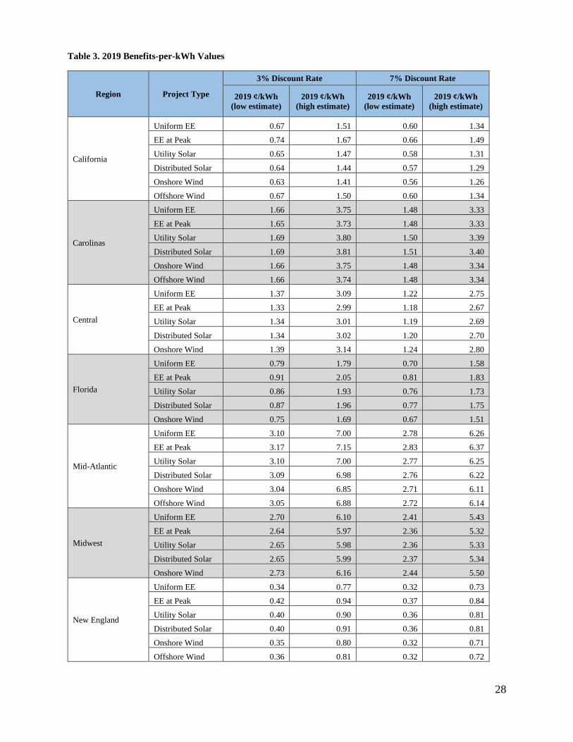
28

Table 3. 2019 Benefits-per-kWh Values

Region Project Type

3% Discount Rate 7% Discount Rate

2019 ¢/kWh

(low estimate)

2019 ¢/kWh

(high estimate)

2019 ¢/kWh

(low estimate)

2019 ¢/kWh

(high estimate)

California

Uniform EE 0.67 1.51 0.60 1.34

EE at Peak 0.74 1.67 0.66 1.49

Utility Solar 0.65 1.47 0.58 1.31

Distributed Solar 0.64 1.44 0.57 1.29

Onshore Wind 0.63 1.41 0.56 1.26

Offshore Wind 0.67 1.50 0.60 1.34

Carolinas

Uniform EE 1.66 3.75 1.48 3.33

EE at Peak 1.65 3.73 1.48 3.33

Utility Solar 1.69 3.80 1.50 3.39


Onshore Wind 1.66 3.75 1.48 3.34

Offshore Wind 1.66 3.74 1.48 3.34

Central

Uniform EE 1.37 3.09 1.22 2.75

EE at Peak 1.33 2.99 1.18 2.67

Utility Solar 1.34 3.01 1.19 2.69


Onshore Wind 1.39 3.14 1.24 2.80

Florida

Uniform EE 0.79 1.79 0.70 1.58

EE at Peak 0.91 2.05 0.81 1.83

Utility Solar 0.86 1.93 0.76 1.73


Onshore Wind 0.75 1.69 0.67 1.51

Mid-Atlantic

Uniform EE 3.10 7.00 2.78 6.26

EE at Peak 3.17 7.15 2.83 6.37

Utility Solar 3.10 7.00 2.77 6.25


Onshore Wind 3.04 6.85 2.71 6.11

Offshore Wind 3.05 6.88 2.72 6.14

Midwest

Uniform EE 2.70 6.10 2.41 5.43

EE at Peak 2.64 5.97 2.36 5.32

Utility Solar 2.65 5.98 2.36 5.33


Onshore Wind 2.73 6.16 2.44 5.50

New England

Uniform EE 0.34 0.77 0.32 0.73

EE at Peak 0.42 0.94 0.37 0.84

Utility Solar 0.40 0.90 0.36 0.81


Onshore Wind 0.35 0.80 0.32 0.71

Offshore Wind 0.36 0.81 0.32 0.72

29

Region Project Type


2019 ¢/kWh

(low estimate)

2019 ¢/kWh

(high estimate)

2019 ¢/kWh

(low estimate)

2019 ¢/kWh

(high estimate)

New York

Uniform EE 0.99 2.24 0.88 1.98

EE at Peak 1.19 2.68 1.06 2.39

Utility Solar 1.10 2.49 0.99 2.22


Onshore Wind 0.95 2.13 0.85 1.90

Offshore Wind 0.94 2.12 0.84 1.89

Northwest

Uniform EE 1.06 2.39 0.95 2.14

EE at Peak 1.11 2.49 0.99 2.22

Utility Solar 1.12 2.53 1.00 2.26


Onshore Wind 1.04 2.35 0.93 2.10

Offshore Wind 1.05 2.38 0.94 2.12

Rocky Mountains

Uniform EE 0.93 2.10 0.82 1.84

EE at Peak 0.91 2.05 0.81 1.83

Utility Solar 0.91 2.05 0.81 1.83


Onshore Wind 0.92 2.08 0.82 1.85

Southeast

Uniform EE 0.69 1.55 0.67 1.51

EE at Peak 0.84 1.90 0.75 1.70

Utility Solar 0.81 1.83 0.72 1.63


Onshore Wind 0.73 1.65 0.65 1.47

Southwest

Uniform EE 0.58 1.31 0.52 1.16

EE at Peak 0.63 1.43 0.56 1.27

Utility Solar 0.61 1.38 0.55 1.23


Onshore Wind 0.57 1.28 0.51 1.14

Tennessee

Uniform EE 0.84 1.89 0.75 1.70

EE at Peak 0.88 1.98 0.78 1.76

Utility Solar 0.84 1.89 0.75 1.68


Onshore Wind 0.82 1.85 0.73 1.65

Texas

Uniform EE 0.91 2.04 0.81 1.83

EE at Peak 0.97 2.18 0.86 1.94

Utility Solar 0.95 2.13 0.85 1.90


Onshore Wind 0.88 1.99 0.79 1.78

30

Discussion The BPK values represent estimates of the monetized annual public health benefits resulting

from emissions reductions associated with EE/RE projects, programs, and policies. There are

different values for each combination of region and EE/RE intervention type (i.e., onshore and

offshore wind, utility and distributed solar, uniform EE, and EE at peak). The total benefits from

EE/RE projects, programs, and policies in any region will include health benefits both within and

outside of that region.

The results show that there are larger differences in BPK across regions than across EE/RE

technologies. This is likely due to differences in the fossil fuel mix used for generation across

regions. For example, New England has low BPK values because its fossil fuel generation comes

almost entirely from natural gas, which has low emissions rates compared to coal. These

emissions rates are similar regardless of the EE/RE technology displacing the fossil fuel

generation. However, in other regions such as the New York, there is more variation in BPK

values across technology types. In the case of the New York, the fossil fuel generation operating

during the peak period has higher emissions rates than the generation operating during other

times of the day. Therefore, EE at peak and solar power, which displace generation during the

daytime peak hours, have higher BPK than wind or uniform EE, which displace generation in

more hours of the day.

However, emissions are only one factor in the estimation of BPK values. The estimated health

benefits are also affected by the population of the areas impacted by the emissions reductions.

Areas with more people affected by changes in air quality will have a greater cumulative health

benefit. For example, the Southwest has higher NOx and PM2.5 emissions rates than New York,

although both regions have similar SO2 rates. However, New York has larger BPK for all

technology types; this is due in part to New York’s higher population density relative to the

Southwest.

In most cases, the regional variation in BPK values is driven by differences in both population

and emissions rates. For example, the Midwest has higher avoided SO2 and NOx emissions rates

compared to the Mid-Atlantic region in 2019. However, the Mid-Atlantic region has nearly 40%

higher BPK values than the Midwest. The likely explanation for this is that Mid-Atlantic region

is more densely populated than the Midwest region.

By generating these health benefits per kWh values for EE/RE, EPA hopes to address the gap in

the literature and provide health BPK values that cover all regions in the United States and cover

key EE/RE project, program, and policy types. Such health benefits estimates may have several

uses. For example, state public utility commissions (PUCs) and state energy offices (SEOs) may

use estimates of the monetized public health benefits of EE as an input to portfolio-level, cost-

benefit analyses; or program-specific, cost-effectiveness tests. Policymakers or financial

institutions could also use these estimates to develop a fuller accounting of the benefits of

investments in EE/RE. Finally, EE/RE developers, state and local public health administrators,

NGOs, and the general public can use these estimates to quantify the public health benefits of

existing or proposed EE/RE projects, programs, and policies. Please note that this is not an

exhaustive list of uses for BPK values. Furthermore, because the BPK values provide a

31

screening-level estimate, they may not be appropriate for certain analyses, such as federal air

quality rulemaking.

In addition, as discussed in the Limitations section on page 22, one area of additional research

includes developing BPK values for future years. Such values would be based on modeling the

electricity sector to estimate emissions rates in future years and would allow for the projection of

benefits from EE/RE projects, programs, and policies in years beyond 2024 (the current limit of

the 2019 values).

Conclusions State and local governments are increasingly interested in quantifying the public health value of

emissions reductions from EE/RE so that they can fully reflect these benefits in policy decision-

making processes. Some studies have quantified the benefits but have used different approaches

and assumptions, making it difficult for others to adopt or credibly compare the health benefits

estimates on a per-kWh basis.

EPA has developed regional-level BPK values to fill the gap for this type of analysis in the

literature. By using the AVERT and COBRA tools, EPA developed regional BPK values for

uniform EE, EE at peak, wind, and solar projects, programs, and policies, which incorporate the

benefits of SO2, NOx, and PM2.5 emissions reductions. Although results vary by region, on

average, EPA found that EE/RE programs delivered benefits of 0.3¢/kWh to 7.2¢/kWh in the

United States in 2019 (using a 3% discount rate).

EPA believes that these values may be useful to a wide range of stakeholders seeking to estimate

public health benefits due to avoided emissions of fine particulate matter (PM2.5) and other

precursor pollutants from EE/RE projects, programs, and policies. Stakeholders may include

state PUCs, SEOs, policymakers, financial institutions, EE/RE developers, state and local public

health administrators, NGOs, and the public.

References Babin, S. M., H. S. Burkom, R. S. Holtry, N. R. Tabernero, L. D. Stokes, J. O. Davies-Cole, K.

DeHaan, and D. H. Lee. 2007. Pediatric patient asthma-related emergency department

visits and admissions in Washington, DC, from 2001-2004, and associations with air

quality, socio-economic status and age group. Environmental Health, 6, 9.

Barbose, G., R. Wiser, J. Heeter, T. Mai, L. Bird, M. Bolinger, A. Carpenter, G. Heath,

D. Keyser, J. Macknick, A. Mills, and D. Millstein. 2016. A retrospective analysis of

benefits and impacts of US renewable portfolio standards. Energy Policy 96:645–660.

Bell, M. L., K. Ebisu, R. D. Peng, J. Walker, J. Samet, S. L. Zeger, and F. Dominici. 2008.

Seasonal and Regional Short-term Effects of Fine Particles on Hospital Admissions in

202 US Counties, 1999–2005. American Journal of Epidemiology, 168(11), 1301–1310.

Bird, L., J. Cochran, and X. Wand. 2014. Wind and Solar Energy Curtailament: Experience and

Practice in the United States. National Renewable Energy Laboratory, Golden, CO.

32

Dockery, D. W., J. Cunningham, A. I. Damokosh, L. M. Neas, J. D. Spengler, P. Koutrakis, and

F. E. Speizer. 1996. Health Effects of Acid Aerosols On North American Children -

Respiratory Symptoms. Environmental Health Perspectives, 104(5), 500–505.

Dockins, C.K., K. Maguire, N. Simon, and M. Sullivan. 2004. Value of Statistical Life Analysis

and Environmental Policy: A White Paper. U.S. Environmental Protection Agency,

National Center for Environmental Economics, Golden, CO.

EPA. 2010. Guidelines for Preparing Economic Analyses. U.S. Environmental Protection

Agency, Washington, DC. Available: https://www.epa.gov/environmental-

economics/guidelines-preparing-economic-analyses.

EPA. 2011. The Benefits and Costs of the Clean Air Act from 1990 to 2020. Final Report –

Rev. A. April. U.S. Environmental Protection Agency Office of Air and Radiation.

Available: https://www.epa.gov/sites/production/files/2015-

07/documents/fullreport_rev_a.pdf.

EPA. 2013. Regulatory Impact Analysis for the Final Revisions to the National Ambient Air

Quality Standards for Particulate Matter. U.S. Environmental Protection Agency.

Available: https://www3.epa.gov/ttnecas1/regdata/RIAs/finalria.pdf.

EPA. 2017. Estimating Public Health Benefits of Energy Efficiency and Clean or Renewable

Energy Interventions: Technical Support for Benefits- and Emissions-Related Software

Models. Prepared by Abt Associates for U.S. Environmental Protection Agency, Office

of Atmospheric Programs.

EPA. 2020a. National Emissions Inventory, 2017. U.S. Environmental Protection Agency.

Available: https://www.epa.gov/air-emissions-inventories/2017-national-emissions-

inventory-nei-data.

EPA. 2020b. Technical Support Document: Preparation of Emissions Inventories for 2016v1

North American Emissions Modeling Platform. U.S. Environmental Protection Agency.

Available: https://www.epa.gov/sites/production/files/2020-

11/documents/2016v1_emismod_tsd_508.pdf

Fann, N., K.R. Baker, and C.M. Fulcher. 2012. Characterizing the PM2.5-related health benefits

of emission reductions for 17 industrial, area and mobile emission sectors across the U.S.

Environment International 49:141–151.

Fann, N., C.M. Fulcher, and B.J. Hubbell. 2009. The influence of location, source, and emission

type in estimates of the human health benefits of reducing a ton of air pollution. Air

Quality, Atmosphere & Health 2:69–176.

Glad, J.A., L.L. Brink, E.O. Talbott, P.C. Lee, X. Xu, M. Saul, and J. Rager. 2012. The

Relationship of Ambient Ozone and PM2.5 Levels and Asthma Emergency Department

Visits: Possible Influence of Gender and Ethnicity. Archives of Environmental &

Occupational Health. 62(2): 103–108.

https://www.epa.gov/environmental-economics/guidelines-preparing-economic-analyses

https://www.epa.gov/environmental-economics/guidelines-preparing-economic-analyses

https://www.epa.gov/sites/production/files/2015-07/documents/fullreport_rev_a.pdf

https://www.epa.gov/sites/production/files/2015-07/documents/fullreport_rev_a.pdf

https://www3.epa.gov/ttnecas1/regdata/RIAs/finalria.pdf

https://www.epa.gov/air-emissions-inventories/2017-national-emissions-inventory-nei-data

https://www.epa.gov/air-emissions-inventories/2017-national-emissions-inventory-nei-data

https://www.epa.gov/sites/production/files/2020-11/documents/2016v1_emismod_tsd_508.pdf

https://www.epa.gov/sites/production/files/2020-11/documents/2016v1_emismod_tsd_508.pdf

33

Health Effects Institute. 2018. State of Global Air 2018. Special Report. Health Effects Institute,

Boston, MA. Available: http://www.stateofglobalair.org/sites/default/files/soga-2018-

report.pdf.

IEI. 2017. Energy Efficiency Trends in the Electric Power Industry. Institute for Electric

Innovation. Available:

http://www.edisonfoundation.net/iei/publications/Documents/IEI_Energy%20Efficiency

%20Report_Dec2017.pdf.

Kloog, I., B.A. Coull, A. Zanobetti, P. Koutrakis, and J.D. Schwartz. 2012. Acute and Chronic

Effects of Particles on Hospital Admissions in New-England. PLoS ONE. 7(4): 1–8.

Krewski, D., M. Jerrett, R. T. Burnett, R. Ma, E. Hughes, Y. Shi, and B. Tempalski. 2009.

Extended follow-up and spatial analysis of the American Cancer Society study linking

particulate air pollution and mortality. Research Reports Health Effects Institute (140), 5–

114; discussion 115–136.

Lepeule J., F. Laden, D. Dockery, and J. Schwartz. 2012. Chronic exposure to fine particles and

mortality: an extended follow-up of the Harvard Six Cities study from 1974 to 2009.

Environmental Health Perspectives, 120(7), 965–970.

Levy, J.I., A.M. Wilson, J.S. Evans, and J.D. Spengler. 2003. Estimation of primary and

secondary particulate matter intake fractions for power plants in Georgia. Environ Sci

Technol 37:5528–5536.

Mai, T., R. Wiser, G. Barbose, L. Bird, J. Heeter, D. Keysey, V. Krishnan, J. Macknick, and

D. Millstein. 2016. A Prospective Analysis of the Costs, Benefits, and Impacts of

US Renewable Portfolio Standards. National Renewable Energy Laboratory and

Lawrence Berkeley National Laboratory, Golden, CO and Berkeley, CA.

Mar, T. F., T. V. Larson, R. A. Stier, C. Claiborn, and J. Q. Koenig. 2004. An analysis of the

association between respiratory symptoms in subjects with asthma and daily air pollution

in Spokane, Washington. Inhalation Toxicology, 16(13), 809–815.

Mar, T. F., J. Q. Koenig, and J. Primomo. 2010. Associations between asthma emergency visits

and particulate matter sources, including diesel emissions from stationary generators in

Tacoma, Washington. Inhalation Toxicology, 22(6), 445–448.

Millstein, D., R. Wiser, M. Bolinger, and G. Barbose. 2017. The climate and air-quality benefits

of wind and solar power in the United States. Nature Energy 2:17134.

Moolgavkar, S. H. 2000a. Air Pollution and Hospital Admissions for Chronic Obstructive

Pulmonary Disease in Three Metropolitan Areas in the United States. Inhalation

Toxicology, 12(Supplement 4), 75–90.

Moolgavkar, S. H. 2000b. Air pollution and hospital admissions for diseases of the circulatory

system in three U.S. metropolitan areas. Journal of the Air & Waste Management

Association, 50(7), 1199–1206.

Muller, N.Z. and R. Mendelsohn. 2018. The Air Pollution Emission Experiments and Policy

Analysis Model (APEEP) Technical Appendix. Yale University School of Forestry and

http://www.stateofglobalair.org/sites/default/files/soga-2018-report.pdf

http://www.stateofglobalair.org/sites/default/files/soga-2018-report.pdf

http://www.edisonfoundation.net/iei/publications/Documents/IEI_Energy%20Efficiency%20Report_Dec2017.pdf

http://www.edisonfoundation.net/iei/publications/Documents/IEI_Energy%20Efficiency%20Report_Dec2017.pdf

34

Environmental Studies, New Haven, CT. Available:

https://www.researchgate.net/profile/Nicholas_Muller/publication/253359043_The_Air_

Pollution_Emission_Experiments_and_Policy_Analysis_Model_APEEP_Technical_App

endix/links/02e7e527248d726274000000/The-Air-Pollution-Emission-Experiments-and-

Policy-Analysis-Model-APEEP-Technical-Appendix.pdf.

Ostro, B. D. 1987. Air Pollution and Morbidity Revisited: A Specification Test. Journal of

Environmental Economics and Management, 14, 87–98.

Ostro, B. D., and S. Rothschild. 1989. Air Pollution and Acute Respiratory Morbidity - an

Observational Study of Multiple Pollutants. Environ Res, 50(2), 238–247.

Ostro, B., M. Lipsett, J. Mann, H. Braxton-Owens, and M. White. 2001. Air pollution and

exacerbation of asthma in African-American children in Los Angeles. Epidemiology,

12(2), 200–208.

Peng, R. D., H. H. Chang, M. L. Bell, A. McDermott, S. L. Zeger, J. M. Samet, and F. Dominici.

2008. Coarse particulate matter air pollution and hospital admissions for cardiovascular

and respiratory diseases among Medicare patients. Jama, 299(18), 2172–2179.

Peng, R. D., M. L. Bell, A. S. Geyh, A. McDermott, S. L. Zeger, J. M. Samet, and F. Dominici.

2009. Emergency admissions for cardiovascular and respiratory diseases and the

chemical composition of fine particle air pollution. Environ Health Perspectives, 117(6),

957–963.

Peters, A., D. W. Dockery, J. E. Muller, and M.A. Mittleman. 2001. Increased particulate air

pollution and the triggering of myocardial infarction. Circulation, 103(23), 2810–2815.

Pope, C. A., D. W. Dockery, J. D. Spengler, and M. E. Raizenne. 1991. Respiratory Health and

Pm10 Pollution - a Daily Time Series Analysis. American Review of Respiratory Disease,

144(3), 668–674.

Pope, C. A., J. B. Muhlestein 3rd, H. T. May, D. G. Renlund, J. L. Anderson, and B. D. Horne.

2006. Ischemic heart disease events triggered by short-term exposure to fine particulate

air pollution. Circulation, 114(23), 2443–2448.

Russell, M. W., D. M. Huse, S. Drowns, E. C. Hamel, and S. C. Hartz. 1998. Direct medical

costs of coronary artery disease in the United States. American Journal of Cardiology,

81(9), 1110–1115.

Schwartz, J., and L. M. Neas. 2000. Fine particles are more strongly associated than coarse

particles with acute respiratory health effects in schoolchildren. Epidemiology, 11(1), 6–

10.

Sheppard, L. 2003. Ambient Air Pollution and Nonelderly Asthma Hospital Admissions in

Seattle, Washington, 1987-1994. In: Revised Analyses of Time-Series Studies of Air

Pollution and Health (pp. 227–230). Boston, MA: Health Effects Institute.

Slaughter, J. C., E. Kim, L. Sheppard, J. H. Sullivan, T. V. Larson, and C. Claiborn. 2005.

Association between particulate matter and emergency room visits, hospital admissions

https://www.researchgate.net/profile/Nicholas_Muller/publication/253359043_The_Air_Pollution_Emission_Experiments_and_Policy_Analysis_Model_APEEP_Technical_Appendix/links/02e7e527248d726274000000/The-Air-Pollution-Emission-Experiments-and-Policy-Analysis-Model-APEEP-Technical-Appendix.pdf




35

and mortality in Spokane, Washington. J Expo Anal Environ Epidemiology, 15(2), 153–

159.

Sullivan, J., L. Sheppard, A. Schreuder, N. Ishikawa, D. Siscovick, and J. Kaufman. 2005.

Relation between short-term fine-particulate matter exposure and onset of myocardial

infarction. Epidemiology, 16(1), 41–48.

U.S. Census Bureau. 2020. County Population by Characteristics: 2010-2019. Available: https://www.census.gov/data/datasets/time-series/demo/popest/2010s-counties-detail.html

Wiser, R., M. Bolinger, G. Heath, D. Keyser, E. Lantz, J. Macknick, T. Mai, and D. Millstein.

2016a. Long-term implications of sustained wind power growth in the United States:

Potential benefits and secondary impacts. Applied Energy 179:146–158.

Wiser, R., T. Mai, D. Millstein, J. Macknick, A. Carpenter, S. Cohen, W. Cole, B. Frew, and

G. Heath. 2016b. On the Path to SunShot: the Environmental and Public Health Benefits

of Achieving High Penetrations of Solar Energy in the United States. National Renewable

Energy Laboratory, Golden, CO.

Wittels, E. H., J. W. Hay, and A.M. Gotto Jr. 1990. Medical costs of coronary artery disease in

the United States. American Journal of Cardiology, 65(7), 432–440.

Woodruff, T. J., J. Grillo, and K.C. Schoendorf. 1997. The relationship between selected causes

of post neonatal infant mortality and particulate air pollution in the United States.

Environmental Health Perspectives, 105(6), 608–612.

Zanobetti, A., and J. Schwartz. 2006. Air pollution and emergency admissions in Boston, MA.

Journal of Epidemiology & Community Health, 60(10), 890-895. doi: 60/10/890 [pii]

10.1136/jech.2005.039834 [doi]

Zanobetti, A., M. Franklin, and J. Schwartz. 2009. Fine particulate air pollution and its

components in association with cause-specific emergency admissions. Environmental

Health 8, 58-60.

https://www.census.gov/data/datasets/time-series/demo/popest/2010s-counties-detail.html

36

Appendix A: AVoided Emissions and geneRation Tool (AVERT) AVERT analyzes changes in fossil fuel-fired electricity generation from solar, wind, and EE

programs in 14 unique regions of the continental United States (Figure A-1).24 The AVERT

regions take into account the fact

that customers’ electricity

demand is met jointly by

generation resources throughout

a region, rather than from a

single power plant.25 AVERT

provides estimates of changes in

NOx, SO2, PM2.5, and CO2

emissions at the regional, state,

and county levels.

In AVERT, the impacts on

emissions from wind and solar

electricity generation are

modeled using the annual

electricity generation capacity in

MWs of the renewable project.

AVERT uses these capacity inputs to estimate the amount of electricity generation (in megawatt-

hours) the project(s) would produce. Capacities can be entered separately for onshore wind,

offshore wind, utility-scale solar, and distributed (rooftop) solar.

AVERT uses hourly data reported to EPA’s CAMD by EGU. Data are available from 2007 to

2019. These data include gross generation; steam output; heat input; and emissions of SO2, NOx,

and CO2. Hourly emissions of PM2.5 are calculated using data from the National Emissions

Inventory.

AVERT uses hourly data on NOx, SO2, and CO2 emissions to estimate the impact of EE/RE

projects, programs, and policies on emissions. AVERT uses the hourly generation data to

determine the probability of whether a particular unit will be operating in a given hour of the

year. The tool also uses hourly emissions data to estimate the emissions from electricity

generation from that unit. AVERT provides built-in assumptions about the capacity factors of RE

technologies to estimate the annual amount of generation an RE project will produce, and the

likely hours in which it will be operating.26 For example, AVERT uses data from the National

Renewable Energy Laboratory to estimate the likely hours of the year a solar project would

generate electricity in each region. Users are able to develop their own site- or region-specific

24 Although in some regions solar or hydroelectricity may be on the margin, AVERT assumes they are must-take

resources and fossil fuel-fired electricity generators are the only generators affected by increased EE/RE.

25 Note that while there are imports and exports of electricity across regions, AVERT does not explicitly model these

transfers.

26 AVERT reflects regional capacity factors for renewable generation, based on actual wind projects from AWS

Truepower and solar projects modeled in the National Renewable Energy Laboratory’s PV Watts tool, reflecting the

availability of sun and wind resources in each region. See Appendix C of AVERT’s user manual for details.

Figure A-1. AVERT Regions.

37

renewable energy load profiles for use in AVERT; however, this study used the built-in capacity

factor assumptions. For EE projects, programs, and policies, the hours of the year they reduce

electricity demand can be input directly by the user or it can be based on the top hours of demand

in each region.

AVERT then determines which fossil fuel units would likely be operating during the hours that

the EE/RE project, program, or policy is operating or reducing demand, to determine the units

that would be displaced by the EE/RE project, program, or policy. AVERT estimates the

emissions reductions that would occur as a result of that displacement based on the emissions

rate at each unit. The resulting estimated reductions in generation and emissions are reported at

the county, state, and regional levels.

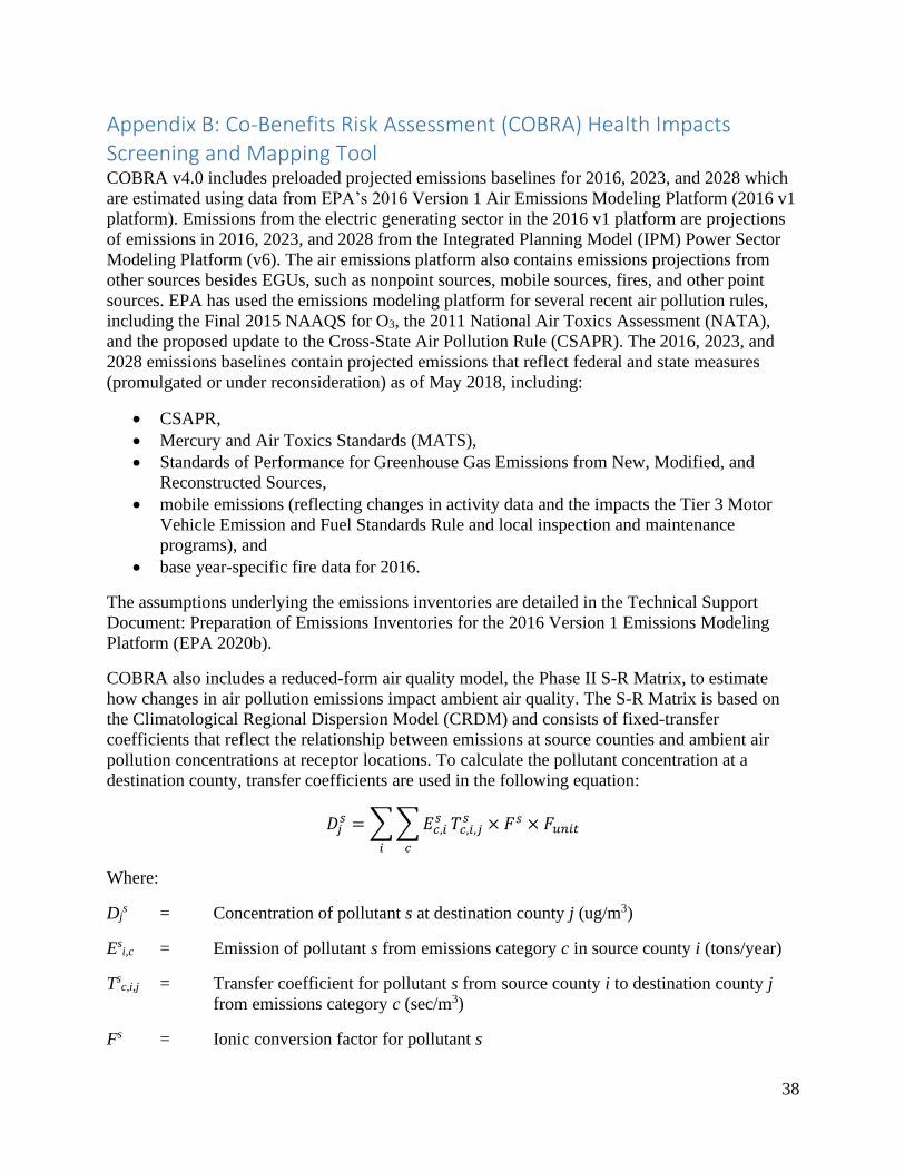
38

Appendix B: Co-Benefits Risk Assessment (COBRA) Health Impacts Screening and Mapping Tool COBRA v4.0 includes preloaded projected emissions baselines for 2016, 2023, and 2028 which

are estimated using data from EPA’s 2016 Version 1 Air Emissions Modeling Platform (2016 v1

platform). Emissions from the electric generating sector in the 2016 v1 platform are projections

of emissions in 2016, 2023, and 2028 from the Integrated Planning Model (IPM) Power Sector

Modeling Platform (v6). The air emissions platform also contains emissions projections from

other sources besides EGUs, such as nonpoint sources, mobile sources, fires, and other point

sources. EPA has used the emissions modeling platform for several recent air pollution rules,

including the Final 2015 NAAQS for O3, the 2011 National Air Toxics Assessment (NATA),

and the proposed update to the Cross-State Air Pollution Rule (CSAPR). The 2016, 2023, and

2028 emissions baselines contain projected emissions that reflect federal and state measures

(promulgated or under reconsideration) as of May 2018, including:

• CSAPR,

• Mercury and Air Toxics Standards (MATS),

• Standards of Performance for Greenhouse Gas Emissions from New, Modified, and

Reconstructed Sources,

• mobile emissions (reflecting changes in activity data and the impacts the Tier 3 Motor

Vehicle Emission and Fuel Standards Rule and local inspection and maintenance

programs), and

• base year-specific fire data for 2016.

The assumptions underlying the emissions inventories are detailed in the Technical Support

Document: Preparation of Emissions Inventories for the 2016 Version 1 Emissions Modeling

Platform (EPA 2020b).

COBRA also includes a reduced-form air quality model, the Phase II S-R Matrix, to estimate

how changes in air pollution emissions impact ambient air quality. The S-R Matrix is based on

the Climatological Regional Dispersion Model (CRDM) and consists of fixed-transfer

coefficients that reflect the relationship between emissions at source counties and ambient air

pollution concentrations at receptor locations. To calculate the pollutant concentration at a

destination county, transfer coefficients are used in the following equation:

𝐷𝑗𝑠 =∑∑𝐸𝑐,𝑖

𝑠

𝑐𝑖

𝑇𝑐,𝑖,𝑗𝑠 × 𝐹𝑠 × 𝐹𝑢𝑛𝑖𝑡

Where:

Djs = Concentration of pollutant s at destination county j (ug/m3)

Esi,c = Emission of pollutant s from emissions category c in source county i (tons/year)

Tsc,i,j = Transfer coefficient for pollutant s from source county i to destination county j

from emissions category c (sec/m3)

Fs = Ionic conversion factor for pollutant s

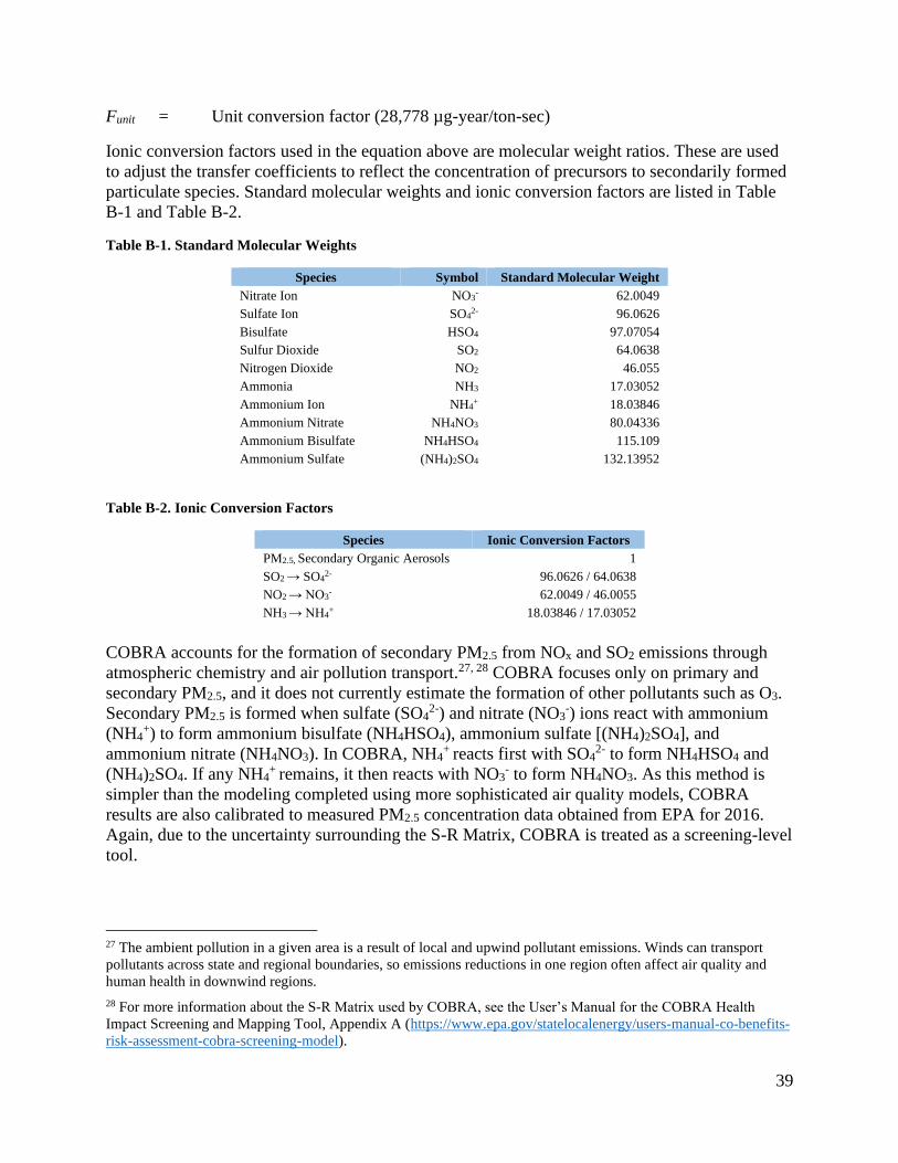
39

Funit = Unit conversion factor (28,778 µg-year/ton-sec)

Ionic conversion factors used in the equation above are molecular weight ratios. These are used

to adjust the transfer coefficients to reflect the concentration of precursors to secondarily formed

particulate species. Standard molecular weights and ionic conversion factors are listed in Table

B-1 and Table B-2.

Table B-1. Standard Molecular Weights

Species Symbol Standard Molecular Weight

Nitrate Ion NO3- 62.0049

Sulfate Ion SO42- 96.0626

Bisulfate HSO4 97.07054

Sulfur Dioxide SO2 64.0638

Nitrogen Dioxide NO2 46.055

Ammonia NH3 17.03052

Ammonium Ion NH4+ 18.03846

Ammonium Nitrate NH4NO3 80.04336

Ammonium Bisulfate NH4HSO4 115.109

Ammonium Sulfate (NH4)2SO4 132.13952

Table B-2. Ionic Conversion Factors

Species Ionic Conversion Factors

PM2.5, Secondary Organic Aerosols 1

SO2 → SO42- 96.0626 / 64.0638

NO2 → NO3- 62.0049 / 46.0055

NH3 → NH4+

18.03846 / 17.03052

COBRA accounts for the formation of secondary PM2.5 from NOx and SO2 emissions through

atmospheric chemistry and air pollution transport.27, 28 COBRA focuses only on primary and

secondary PM2.5, and it does not currently estimate the formation of other pollutants such as O3.

Secondary PM2.5 is formed when sulfate (SO42-) and nitrate (NO3

-) ions react with ammonium

(NH4+) to form ammonium bisulfate (NH4HSO4), ammonium sulfate [(NH4)2SO4], and

ammonium nitrate (NH4NO3). In COBRA, NH4+ reacts first with SO4

2- to form NH4HSO4 and

(NH4)2SO4. If any NH4+ remains, it then reacts with NO3

- to form NH4NO3. As this method is

simpler than the modeling completed using more sophisticated air quality models, COBRA

results are also calibrated to measured PM2.5 concentration data obtained from EPA for 2016.

Again, due to the uncertainty surrounding the S-R Matrix, COBRA is treated as a screening-level

tool.

27 The ambient pollution in a given area is a result of local and upwind pollutant emissions. Winds can transport

pollutants across state and regional boundaries, so emissions reductions in one region often affect air quality and

human health in downwind regions.

28 For more information about the S-R Matrix used by COBRA, see the User’s Manual for the COBRA Health

Impact Screening and Mapping Tool, Appendix A (https://www.epa.gov/statelocalenergy/users-manual-co-benefits-

risk-assessment-cobra-screening-model).



40

Once COBRA estimates the changes in PM2.5 concentrations at the county level, it then uses C-R

functions to determine the change in public health impacts from a change in ambient air quality.

The C-R functions embedded in COBRA are taken from epidemiological studies; and are

consistent with the methods used by EPA to estimate the health impacts of air pollution rules,

including MATS.29 The output of these functions is the number of avoided premature deaths,

heart attacks, hospital admissions for respiratory and cardiovascular-related illnesses, incidences

of acute bronchitis, upper and lower respiratory symptoms, asthma exacerbations or emergency

room visits, minor restricted activity days, and illness-related work loss days. See Appendix E for

a list of the epidemiological studies and more information about the C-R function used in

COBRA.

Finally, COBRA applies estimates of the value of avoiding public health impacts to determine

the monetary benefits associated with reductions in air pollution. Values used in COBRA were

used in recent EPA RIAs, including analyses for the rule mentioned above. They were derived

using a variety of methods that estimate how much people are willing to pay to reduce the risk of

a health incident or the cost of illness (COI), which includes direct medical costs and opportunity

costs.30 The value of avoiding premature adult mortality, also known as the value of a statistical

life (VSL), is generally responsible for more than 95% of the monetized benefits of emissions

reductions. The VSL used in COBRA to estimate the value of avoided adult mortality ranges

from approximately $8.7 million to $9.7 million (in 2017 USD), assuming a discount rate of 7%

and 3%, respectively. This VSL value, based on 26 published studies, is identical to the values

used by EPA in regulatory analyses of air pollution rules. The value of other health impacts, such

as non-fatal heart attacks, hospitalizations, and asthma exacerbations, are smaller and based on

the COI. For example, the value of non-fatal heart attacks ranges between $37,038 and $309,825,

and the value of hospital admissions ranges between $17,655 and $47,581 per incident. See

Appendix G for a complete list of the values used in COBRA.

29 For a complete list of recent RIAs of EPA air pollution rules, see https://www.epa.gov/economic-and-cost-

analysis-air-pollution-regulations/regulatory-impact-analyses-air-pollution. Many of these analyses use a BPT

approach, developed by EPA (Fann et al. 2012). COBRA uses most of the same C-R functions as those used in the

BPT approach. For a list and description of the epidemiological studies used by COBRA to estimate adverse health

effects, see the User’s Manual for the COBRA Health Impact Screening and Mapping Tool, Appendix C

(https://www.epa.gov/statelocalenergy/users-manual-co-benefits-risk-assessment-cobra-screening-model).

30 For more information about the economic values used by COBRA to estimate the economic value of avoiding

adverse health effects and how they were derived, see the User’s Manual for the COBRA Health Impact Screening

and Mapping Tool, Appendix F (https://www.epa.gov/statelocalenergy/users-manual-co-benefits-risk-assessment-

cobra-screening-model).






41

Appendix C: Sensitivity Analyses on Project, Program, or Policy Size and Peak Energy-Efficiency Definition EPA conducted sensitivity analyses using AVERT and the COBRA tool to determine the extent

to which modeling scenario assumptions might impact the BPK results. EPA analyzed

two different types of potential sensitivity: the size of the EE/RE project, program, or policy

studied; and the definition of EE at peak.

EPA conducted this sensitivity analysis for the original 2017 BPK values. The sensitivity

analysis was not updated for the 2019 values.

Sensitivity Analysis on Project, Program, or Policy Size Assumptions EPA examined the potential sensitivity of the BPK values to assumptions about project size by

modeling BPK values for five different project sizes: from 100 MW to 2,000 MW added

capacity for the wind and utility solar modeling options in AVERT, and from 100 GWh to

2,000 GWh of displaced generation for the EE modeling options.

The results of these model runs illustrate that there is a strong linear relationship between project

size and emissions reductions (R2 = 0.9996–1.0, Figure C-1). The results from AVERT were

then input into COBRA to assess the sensitivity of emissions reductions on health impacts. These

results also show that there is a strong linear relationship between the amount of emissions

reductions and health impacts (Figure C - 2).

The results of this sensitivity analysis indicate that the project size does not have a large impact

on the marginal BPK results (i.e., a larger project does not generate disproportionately larger

marginal benefits or have a higher BPK result than a smaller project). The resulting BPK values

from these model runs with different project sizes are consistent with this; for each region and

project, program, or policy type modeled, the results are within 0.1¢ per kWh (Table C-1). As a

result, this analysis presents BPK values modeled using only a single assumption about project

size.

Note, however, an extremely large EE/RE project, program, or policy could displace more than

the marginal EGUs and extend into the baseload units, which may have a different emissions

profile. See the Limitations section on page 22 of this report for more information about the

limitations on project size for which the BPK values should be used.

42

Figure C-1. AVERT Sensitivity for Project, Program, or Policy Size.

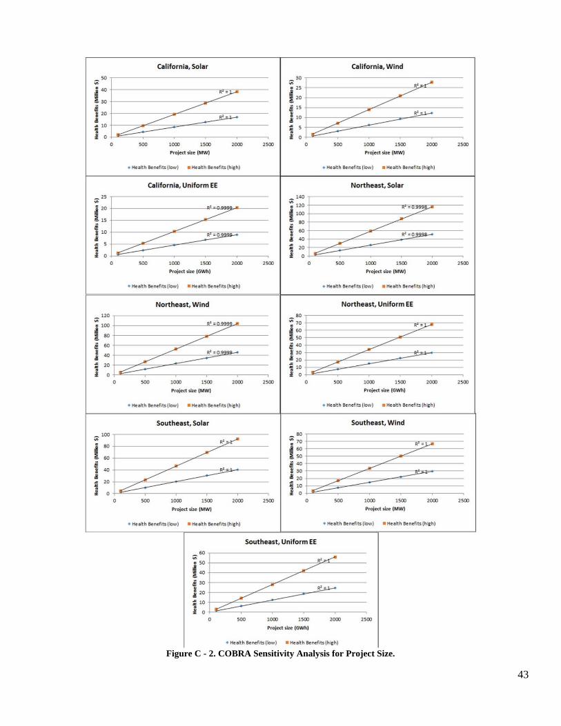
43

Figure C - 2. COBRA Sensitivity Analysis for Project Size.

44

Table C-1. Results from Sensitivity Analysis on Project, Program, or Policy Size

Emissions Reductions (tons) from

AVERT

Health Benefits (million USD)

from COBRA Benefits per kWh (¢/kWh)

Region Project Type Capacity

(MW/GWh)

Displaced

Generation

(MWh)

SO2 NOx PM2.5 Health Benefits

(low)

Health Benefits

(high) Low Estimate High Estimate

Southeast

Wind

100 120,370 84 56 6 1.67 3.77 1.4 3.1

500 602,150 418 281 30 8.33 18.86 1.4 3.1

1,000 1,204,500 837 562 60 16.60 37.58 1.4 3.1

1,500 1,806,580 1,256 842 91 24.85 56.25 1.4 3.1

2,000 2,408,940 1,676 1,124 121 33.06 74.83 1.4 3.1

Solar

100 169,440 121 90 9 2.33 5.28 1.4 3.1

500 847,250 601 449 46 11.52 26.08 1.4 3.1

1,000 1,694,380 1,205 897 92 22.96 51.98 1.4 3.1

1,500 2,541,750 1,807 1,342 137 34.27 77.57 1.3 3.1

2,000 3,388,780 2,408 1,788 183 45.52 103.04 1.3 3.0

Uniform EE

100 104,950 72 51 5 1.40 3.17 1.3 3.0

500 524,940 359 257 27 6.99 15.81 1.3 3.0

1,000 1,049,980 716 514 54 13.90 31.47 1.3 3.0

1,500 1,575,040 1,073 771 82 20.79 47.06 1.3 3.0

2,000 2,099,990 1,432 1,027 109 27.64 62.57 1.3 3.0

California

Wind

100 152,050 5 26 3 0.75 1.69 0.5 1.1

500 761,630 25 129 15 3.55 8.02 0.5 1.1

1,000 1,522,830 50 257 30 6.93 15.67 0.5 1.0

1,500 2,284,090 75 386 45 10.35 23.39 0.5 1.0

2,000 3,044,890 99 514 60 13.75 31.09 0.5 1.0

Solar

100 194,640 6 36 4 1.04 2.34 0.5 1.2

500 971,730 31 174 19 4.84 10.94 0.5 1.1

1,000 1,945,550 62 346 39 9.51 21.50 0.5 1.1

1,500 2,923,700 93 523 59 14.26 32.22 0.5 1.1

2,000 3,899,550 126 704 79 18.98 42.93 0.5 1.1

Uniform EE

100 104,510 3 19 2 0.56 1.27 0.5 1.2

500 522,680 17 94 10 2.65 5.99 0.5 1.1

1,000 1,045,830 34 187 21 5.13 11.59 0.5 1.1

1,500 1,568,940 51 279 31 7.59 17.16 0.5 1.1

2,000 2,091,230 68 369 41 10.02 22.66 0.5 1.1

45

Emissions Reductions (tons) from

AVERT

Health Benefits (million USD)

from COBRA Benefits per kWh (¢/kWh)

Region Project Type Capacity

(MW/GWh)

Displaced

Generation

(MWh)

SO2 NOx PM2.5 Health Benefits

(low)

Health Benefits

(high) Low Estimate High Estimate

Northeast

Wind

100 174,470 29 37 3 2.72 6.14 1.6 3.5

500 873,200 141 187 17 13.37 30.20 1.5 3.5

1,000 1,748,100 275 369 35 26.24 59.26 1.5 3.4

1,500 2,620,800 407 549 52 38.81 87.64 1.5 3.3

2,000 3,495,010 537 727 69 51.37 116.02 1.5 3.3

Solar

100 157,170 32 46 4 3.01 6.72 1.9 4.3

500 787,140 157 227 19 14.83 33.50 1.9 4.3

1,000 1,573,340 306 448 39 29.42 66.45 1.9 4.2

1,500 2,361,630 449 660 58 43.65 98.56 1.8 4.2

2,000 3,146,030 590 869 77 57.51 129.88 1.8 4.1

Uniform EE

100 104,880 18 25 2 1.72 3.91 1.6 3.7

500 524,150 88 126 11 8.57 19.36 1.6 3.7

1,000 1,048,680 175 252 23 16.99 38.36 1.6 3.7

1,500 1,573,550 262 377 34 25.31 57.15 1.6 3.6

2,000 2,098,790 347 501 45 33.58 75.85 1.6 3.6

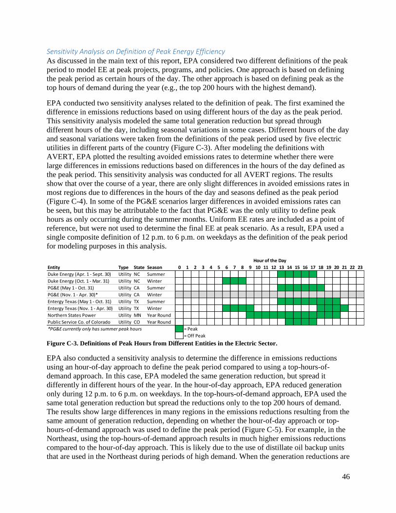
46

Sensitivity Analysis on Definition of Peak Energy Efficiency As discussed in the main text of this report, EPA considered two different definitions of the peak

period to model EE at peak projects, programs, and policies. One approach is based on defining

the peak period as certain hours of the day. The other approach is based on defining peak as the

top hours of demand during the year (e.g., the top 200 hours with the highest demand).

EPA conducted two sensitivity analyses related to the definition of peak. The first examined the

difference in emissions reductions based on using different hours of the day as the peak period.

This sensitivity analysis modeled the same total generation reduction but spread through

different hours of the day, including seasonal variations in some cases. Different hours of the day

and seasonal variations were taken from the definitions of the peak period used by five electric

utilities in different parts of the country (Figure C-3). After modeling the definitions with

AVERT, EPA plotted the resulting avoided emissions rates to determine whether there were

large differences in emissions reductions based on differences in the hours of the day defined as

the peak period. This sensitivity analysis was conducted for all AVERT regions. The results

show that over the course of a year, there are only slight differences in avoided emissions rates in

most regions due to differences in the hours of the day and seasons defined as the peak period

(Figure C-4). In some of the PG&E scenarios larger differences in avoided emissions rates can

be seen, but this may be attributable to the fact that PG&E was the only utility to define peak

hours as only occurring during the summer months. Uniform EE rates are included as a point of

reference, but were not used to determine the final EE at peak scenario. As a result, EPA used a

single composite definition of 12 p.m. to 6 p.m. on weekdays as the definition of the peak period

for modeling purposes in this analysis.

Figure C-3. Definitions of Peak Hours from Different Entities in the Electric Sector.

EPA also conducted a sensitivity analysis to determine the difference in emissions reductions

using an hour-of-day approach to define the peak period compared to using a top-hours-of-

demand approach. In this case, EPA modeled the same generation reduction, but spread it

differently in different hours of the year. In the hour-of-day approach, EPA reduced generation

only during 12 p.m. to 6 p.m. on weekdays. In the top-hours-of-demand approach, EPA used the

same total generation reduction but spread the reductions only to the top 200 hours of demand.

The results show large differences in many regions in the emissions reductions resulting from the

same amount of generation reduction, depending on whether the hour-of-day approach or top-

hours-of-demand approach was used to define the peak period (Figure C-5). For example, in the

Northeast, using the top-hours-of-demand approach results in much higher emissions reductions

compared to the hour-of-day approach. This is likely due to the use of distillate oil backup units

that are used in the Northeast during periods of high demand. When the generation reductions are

Entity Type State Season 0 1 2 3 4 5 6 7 8 9 10 11 12 13 14 15 16 17 18 19 20 21 22 23

Duke Energy (Apr. 1 - Sept. 30) Utility NC Summer

Duke Energy (Oct. 1 - Mar. 31) Utility NC Winter

PG&E (May 1 - Oct. 31) Utility CA Summer

PG&E (Nov. 1 - Apr. 30)* Utility CA Winter

Entergy Texas (May 1 - Oct. 31) Utility TX Summer

Entergy Texas (Nov. 1 - Apr. 30) Utility TX Winter

Northern States Power Utility MN Year Round

Public Service Co. of Colorado Utility CO Year Round

*PG&E currently only has summer peak hours = Peak

= Off Peak

Hour of the Day

47

confined only to this period, it affects only these high-emitting units. Nevertheless, as discussed

in the report, EPA chose to use the hour-of-day approach to define the peak period, as EPA

determined it to be the more relevant definition for most EE/RE projects, programs, and policies

based on expected uses for the BPK values.

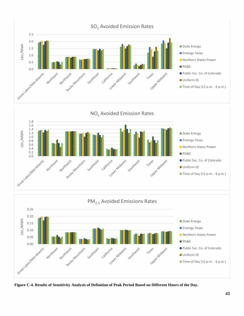
48

Figure C-4. Results of Sensitivity Analysis of Definition of Peak Period Based on Different Hours of the Day.

0.0

0.5

1.0

1.5

2.0

2.5

Lbs.

/Mw

h

SO2 Avoided Emission Rates

Duke Energy

Entergy Texas

Northern States Power

PG&E

Public Svc. Co. of Colorado

Uniform EE

Time of Day (12 p.m. - 6 p.m.)

0.00.20.40.60.81.01.21.41.61.8

Lbs.

/MW

h

NOx Avoided Emission Rates

Duke Energy

Entergy Texas


PG&E


Uniform EE


0.00

0.05

0.10

0.15

0.20

0.25

Lbs.

/MW

h

PM2.5 Avoided Emissions Rates

Duke Energy

Entergy Texas


PG&E


Uniform EE


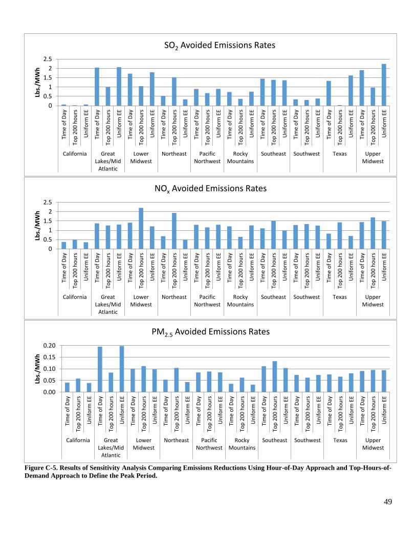
49

Figure C-5. Results of Sensitivity Analysis Comparing Emissions Reductions Using Hour-of-Day Approach and Top-Hours-of-

Demand Approach to Define the Peak Period.

0

0.5

1

1.5

2

2.5Ti

me

of

Day

Top

20

0 h

ou

rs

Un

ifo

rm E

E

Tim

e o

f D

ay

Top

20

0 h

ou

rs

Un

ifo

rm E

E

Tim

e o

f D

ay

Top

20

0 h

ou

rs

Un

ifo

rm E

E

Tim

e o

f D

ay

Top

20

0 h

ou

rs

Un

ifo

rm E

E

Tim

e o

f D

ay

Top

20

0 h

ou

rs

Un

ifo

rm E

E

Tim

e o

f D

ay

Top

20

0 h

ou

rs

Un

ifo

rm E

E

Tim

e o

f D

ay

Top

20

0 h

ou

rs

Un

ifo

rm E

E

Tim

e o

f D

ay

Top

20

0 h

ou

rs

Un

ifo

rm E

E

Tim

e o

f D

ay

Top

20

0 h

ou

rs

Un

ifo

rm E

E

Tim

e o

f D

ay

Top

20

0 h

ou

rs

Un

ifo

rm E

E

California GreatLakes/Mid

Atlantic

LowerMidwest

Northeast PacificNorthwest

RockyMountains

Southeast Southwest Texas UpperMidwest

Lbs.

/MW

h

SO2 Avoided Emissions Rates

0

0.5

1

1.5

2

2.5

Tim

e o

f D

ay

Top

20

0 h

ou

rs

Un

ifo

rm E

E

Tim

e o

f D

ay

Top

20

0 h

ou

rs

Un

ifo

rm E

E

Tim

e o

f D

ay

Top

20

0 h

ou

rs

Un

ifo

rm E

E

Tim

e o

f D

ay

Top

20

0 h

ou

rs

Un

ifo

rm E

E

Tim

e o

f D

ay

Top

20

0 h

ou

rs

Un

ifo

rm E

E

Tim

e o

f D

ay

Top

20

0 h

ou

rs

Un

ifo

rm E

E

Tim

e o

f D

ay

Top

20

0 h

ou

rs

Un

ifo

rm E

E

Tim

e o

f D

ay

Top

20

0 h

ou

rs

Un

ifo

rm E

E

Tim

e o

f D

ay

Top

20

0 h

ou

rs

Un

ifo

rm E

E

Tim

e o

f D

ay

Top

20

0 h

ou

rs

Un

ifo

rm E

E


Atlantic

LowerMidwest


RockyMountains


Lbs.

/MW

h

NOx Avoided Emissions Rates

0.00

0.05

0.10

0.15

0.20

Tim

e o

f D

ay

Top

20

0 h

ou

rs

Un

ifo

rm E

E

Tim

e o

f D

ay

Top

20

0 h

ou

rs

Un

ifo

rm E

E

Tim

e o

f D

ay

Top

20

0 h

ou

rs

Un

ifo

rm E

E

Tim

e o

f D

ay

Top

20

0 h

ou

rs

Un

ifo

rm E

E

Tim

e o

f D

ay

Top

20

0 h

ou

rs

Un

ifo

rm E

E

Tim

e o

f D

ay

Top

20

0 h

ou

rs

Un

ifo

rm E

E

Tim

e o

f D

ay

Top

20

0 h

ou

rs

Un

ifo

rm E

E

Tim

e o

f D

ay

Top

20

0 h

ou

rs

Un

ifo

rm E

E

Tim

e o

f D

ay

Top

20

0 h

ou

rs

Un

ifo

rm E

E

Tim

e o

f D

ay

Top

20

0 h

ou

rs

Un

ifo

rm E

E


Atlantic

LowerMidwest


RockyMountains


Lbs.

/MW

h

PM2.5 Avoided Emissions Rates

50

Appendix D: Top 200 Hours of Demand Benefit-per-kWh Results Table D-1 includes the complete modeling results from AVERT and COBRA used to calculate the BPK values for the top 200 hours of demand

analysis in each region.

EPA conducted this sensitivity analysis for the original 2017 BPK values. The sensitivity analysis was not updated for the 2019 values.

Table D-1. Complete AVERT and COBRA Results for Top 200 Hours of Demand Analysis (3% and 7% discount rate; 2017 USD)

Region Discount

Rate

Results from AVERT SO2

Emissions

Rate

(lbs./MWh)

NOX

Emissions

Rate

(lbs./MWh)

PM2.5

Emissions

Rate

(lb./MWh)

Results from COBRA

¢/kWh

(low)

¢/kWh

(high) Displaced

Generation

(MWh)

SO2

Reduced

(lbs.)

NOX

Reduced

(lbs.)

PM2.5

Reduced

(lbs.)

$ Total Health

Benefits (low)

$ Total Health

Benefits

(high)

California 3 200,230 3,680 33,130 9,530 0.01838 0.16546 0.04760 1,868,183.33 4,221,243.69 0.93 2.11

Great Lakes/Mid-Atlantic 3 205,510 217,960 233,420 35,760 1.06058 1.13581 0.17401 7,353,520.30 16,631,254.33 3.58 8.09

Lower Midwest 3 203,670 3,080 373,040 16,210 0.01512 1.83159 0.07959 1,679,175.59 3,798,562.75 0.82 1.87

Northeast 3 197,440 171,450 210,820 15,640 0.86837 1.06777 0.07921 9,242,207.78 20,874,650.58 4.68 10.57

Pacific Northwest 3 202,330 173,090 228,080 18,200 0.85548 1.12727 0.08995 2,198,711.54 4,972,898.14 1.09 2.46

Rocky Mountains 3 195,720 63,550 226,500 11,870 0.32470 1.15727 0.06065 1,602,727.29 3,625,354.74 0.82 1.85

Southeast 3 201,440 152,400 248,990 24,350 0.75655 1.23605 0.12088 4,045,381.73 9,155,691.94 2.01 4.55

Southwest 3 193,640 7,450 265,600 13,160 0.03847 1.37162 0.06796 1,398,221.15 3,163,872.51 0.72 1.63

Texas 3 197,530 59,330 261,410 13,400 0.30036 1.32339 0.06784 2,243,773.58 5,075,140.16 1.14 2.57

Upper Midwest 3 205,770 133,580 256,210 20,200 0.64917 1.24513 0.09817 3,150,193.28 7,124,723.56 1.53 3.46

California 7 200,230 3,680 33,130 9,530 0.01838 0.16546 0.04760 1,667,429.97 3,765,217.37 0.83 1.88

Great Lakes/Mid-Atlantic 7 205,510 217,960 233,420 35,760 1.06058 1.13581 0.17401 6,561,493.57 14,833,891.17 3.19 7.22

Lower Midwest 7 203,670 3,080 373,040 16,210 0.01512 1.83159 0.07959 1,498,471.30 3,388,096.40 0.74 1.66

Northeast 7 197,440 171,450 210,820 15,640 0.86837 1.06777 0.07921 8,248,584.90 18,620,340.06 4.18 9.43

Pacific Northwest 7 202,330 173,090 228,080 18,200 0.85548 1.12727 0.08995 1,962,089.91 4,435,443.96 0.97 2.19

Rocky Mountains 7 195,720 63,550 226,500 11,870 0.32470 1.15727 0.06065 1,430,318.98 3,233,616.56 0.73 1.65

Southeast 7 201,440 152,400 248,990 24,350 0.75655 1.23605 0.12088 3,609,761.12 8,166,235.14 1.79 4.05

Southwest 7 193,640 7,450 265,600 13,160 0.03847 1.37162 0.06796 1,247,815.35 2,821,961.89 0.64 1.46

Texas 7 197,530 59,330 261,410 13,400 0.30036 1.32339 0.06784 2,002,718.23 4,527,067.37 1.01 2.29

Upper Midwest 7 205,770 133,580 256,210 20,200 0.64917 1.24513 0.09817 2,811,049.78 6,354,838.97 1.37 3.09

51

Appendix E: Health Impact Functions The health impact functions in the COBRA model were prepared by Abt Associates in close

consultation with EPA, and rely on an up-to-date assessment of the published scientific literature

to ascertain the relationship between ambient PM2.5 concentrations and adverse human health

effects. Table E–1 summarizes the key values from the epidemiological studies in COBRA used

to estimate adverse health impacts of PM2.5. The output of each health impact function is the

estimated number of incidences of each health outcome given a change in air pollution

concentrations.

Total results in COBRA and in this report are reported for a low and high estimate of health

impacts, which is a result of multiple C-R functions being used to calculate mortality and

nonfatal heart attacks. The high estimate uses the Lepeule et al. (2012) mortality estimate and the

Peters et al. (2001) non-fatal heart attack estimates. The low estimate uses the Krewski et al.

(2009) mortality estimates and the remaining four acute myocardial infarction estimates. See

Appendix C of the COBRA User’s Manual for more information.

Table E-1. Key Health Impact Values in COBRA

Endpoint Author Age Location Metric Beta Standard

Error

Functional

Form

Mortality, All Cause Krewski et al. (2009) 30–99 116 U.S. cities Annual 0.005827 0.000963 Log-linear

Mortality, All Cause Lepeule et al. (2012) 25–99 6 eastern cities Annual 0.013103 0.003347 Log-linear

Mortality, All Cause Woodruff et al.

(1997) Infant 86 cities Annual 0.003922 0.001221 Logistic

Acute Myocardial

Infarction, Nonfatal Peters et al. (2001) 18–99 Boston, MA

24-hour

average 0.024121 0.009285 Logistic

Acute Myocardial

Infarction, Nonfatal Pope et al. (2006) 18–99

Greater Salt

Lake City, Utah

24-hour


Acute Myocardial

Infarction, Nonfatal Sullivan et al. (2005) 18–99

King County,

Washington

24-hour


Acute Myocardial

Infarction, Nonfatal

Zanobetti and

Schwartz (2006) 18–99

Greater Boston

area

24-hour


Acute Myocardial

Infarction, Nonfatal

Zanobetti et al.

(2009) 18–99

26 U.S.

communities

24-hour

average 0.00225 0.000592 Log-linear

Hospital Admissions, All

Cardiovascular (less

myocardial infarctions)

Bell et al. (2008) 65–99 202 U.S.

counties

24-hour





Moolgavkar (2000b) 18–64 Los Angeles,

CA

24-hour





Peng et al. (2008) 65–99 108 U.S.

counties

24-hour





Peng et al. (2009) 65–99 119 U.S. urban

counties

24-hour





Zanobetti et al.

(2009) 65–99

26 U.S.

communities

24-hour



Respiratory

Zanobetti et al.

(2009) 65–99

26 U.S.

communities

24-hour


52

Endpoint Author Age Location Metric Beta Standard

Error

Functional

Form


Respiratory Kloog et al. (2012) 65–99

New England

area (6 states)

24-hour


Hospital Admissions,

Asthma Babin et al. (2007) 0–17

Washington,

DC

24-hour



Asthma Sheppard (2003) 0–17 Seattle, WA

24-hour



Chronic Lung Disease Moolgavkar (2000a) 18–64

Los Angeles,

CA

24-hour


Emergency Room Visits,

Asthma Mar et al. (2010) 0–99

Greater

Tacoma,

Washington

24-hour



Asthma

Slaughter et al.

(2005) 0–99

Spokane,

Washington

24-hour



Asthma Glad et al. (2012) 0–99 Pittsburgh, PA

24-hour


Acute Bronchitis Dockery et al. (1996) 8–12 24 communities Annual 0.027212 0.017096 Logistic

Asthma Exacerbation,

Cough Mar et al. (2004) 6–18

Vancouver,

CAN

24-hour



Cough Ostro et al. (2001) 6–18

Los Angeles,

CA

24-hour



Shortness of Breath Mar et al. (2004) 6–18

Vancouver,

CAN

24-hour



Shortness of Breath Ostro et al. (2001) 6–18

Los Angeles,

CA

24-hour



Wheeze Ostro et al. (2001) 6–18

Los Angeles,

CA

24-hour


Minor Restricted Activity

Days

Ostro and Rothschild

(1989) 18–64 Nationwide

24-hour


Lower Respiratory

Symptoms

Schwartz and Neas

(2000) 7–14 6 U.S. cities

24-hour


Upper Respiratory

Symptoms Pope et al. (1991) 9–11 Utah Valley

24-hour


Work Loss Days Ostro (1987) 18–64 Nationwide 24-hour


53

Appendix F: Health Benefits Valuation Table F–1 presents the mean estimate of the unit values used in COBRA to estimate the

monetary value of the health effects. The unit values are based on published estimates of the

costs of treating the illness (which can include both direct medical costs and costs of lost

productivity), or the willingness-to-pay (WTP) to avoid the illness or to reduce the risk of

premature death (i.e., VSL). The unit values based on WTP estimates reflect the expected growth

in real income over time. This is consistent with economic theory, which argues that WTP for

most goods (such as health risk reductions) will increase if real incomes increase. See Appendix

F of the COBRA User’s Manual for more information. The values shown in Table F–1 are

interpolated between the unit values for 2016 and 2023 from COBRA.

Table F-1. COBRA Value of Health Effects

a Mortality value after adjustment for 20-year lag. b Infant mortality value is not adjusted for 20-year lag. c Based on Russell et al. (1998). d Based on Wittels et al. (1990).

Health Endpoint Age

Range

Unit Value (2017 USD at the 2019 income level)


Mortalitya 25–99 $ 9,595,710 $8,546,746

Infant Mortalityb 0–0 $10,695,507 $10,695,507

Acute Myocardial Infarction, Nonfatalc 0–24 $39,174 $37,038





Acute Myocardial Infarction, Nonfatald 0–24 $192,048 $192,048





Hospital Admissions, All Cardiovascular (less-acute

myocardinal infraction) 18–64

$47,581 $47,581

Hospital Admissions, All Cardiovascular (less-acute

myocardinal infraction) 65–99

$44,642 $44,642

Hospital Admissions, All Respiratory 65–99 $37,463 $37,463

Hospital Admissions, Asthma 0–17 $17,655 $17,655

Hospital Admissions, Chronic Lung Disease 18–64 $23,294 $23,294

Asthma Emergency Room Visits (Smith et al. 1997) 0–99 $547 $547

Asthma Emergency Room Visits (Stanford et al. 1999) 0–99 $457 $457

Acute Bronchitis 8–12 $546 $546

Lower Respiratory Symptoms 7–14 $24 $24

Upper Respiratory Symptoms 9–11 $38 $38

Minor Restricted Activity Days 18–64 $78 $78

Work Loss Days 18–64 $178 $178

Asthma Exacerbation (cough, shortness of breath, or

wheeze) 6–18

$66 $66

54

Appendix G: Detailed Benefits-per-kWh Results Table G–1 includes the complete modeling results from AVERT and COBRA used to calculate the BPK values for each region and technology type.

Table G-1. Complete AVERT and COBRA Results for 2019 (3% and 7% discount rate)

Region Project Type Discount

Rate


Emissions

Rate

(lb./MWh)

NOx

Emissions

Rate

(lb./MWh)

PM25

Emissions

Rate

(lb./MWh)

Results from COBRA

¢/kWh

(low) ¢/kWh

(high) Displaced

Generation

(MWh)

SO2

Reduced

(lbs.)

NOx

Reduced

(lbs.)

PM25

Reduced

(lbs.)

$ Total

Health

Benefits

$ Total

Health

Benefits

(low) (high)

California Uniform EE 3 547,340 30,060 137,320 20,880 0.055 0.251 0.038 3,664,818 8,241,303 0.67 1.51

California EE at Peak 3 218,816 12,010 56,420 8,540 0.055 0.258 0.039 1,627,609 3,659,655 0.74 1.67

California Utility Solar 3 232,688 11,800 56,400 8,790 0.051 0.242 0.038 1,517,888 3,413,326 0.65 1.47

California

Distributed

Solar 3 200,500 10,154 48,136 7,542 0.051 0.240 0.038 1,288,019 2,896,454 0.64 1.44

California

Onshore

Wind 3 151,734 7,930 36,580 5,690 0.052 0.241 0.037 954,668 2,146,941 0.63 1.41

California

Offshore

Wind 3 263,330 13,554 63,440 9,928 0.051 0.241 0.038 1,762,325 3,962,872 0.67 1.50

Carolinas Uniform EE 3 537,690 321,240 498,030 60,400 0.597 0.926 0.112 8,950,290 20,189,459 1.66 3.75

Carolinas EE at Peak 3 215,513 124,420 205,620 24,410 0.577 0.954 0.113 3,564,985 8,041,621 1.65 3.73

Carolinas Utility Solar 3 194,688 117,240 181,900 22,050 0.602 0.934 0.113 3,281,253 7,401,623 1.69 3.80

Carolinas

Distributed

Solar 3 166,870 100,354 156,788 18,934 0.601 0.940 0.113 2,817,368 6,355,224 1.69 3.81

Carolinas

Onshore

Wind 3 120,474 70,430 112,330 13,310 0.585 0.932 0.110 2,002,200 4,516,442 1.66 3.75

Carolinas

Offshore

Wind 3 244,230 143,772 229,740 27,260 0.589 0.941 0.112 4,048,304 9,131,907 1.66 3.74

Central Uniform EE 3 539,450 678,890 642,870 42,000 1.258 1.192 0.078 7,401,437 16,687,926 1.37 3.09

Central EE at Peak 3 215,513 245,840 279,290 17,380 1.141 1.296 0.081 2,858,322 6,444,562 1.33 2.99

Central Utility Solar 3 225,810 266,470 284,790 17,860 1.180 1.261 0.079 3,016,605 6,801,469 1.34 3.01

Central

Distributed

Solar 3 190,820 225,580 242,526 15,160 1.182 1.271 0.079 2,559,365 5,770,535 1.34 3.02

Central

Onshore

Wind 3 351,609 458,062 412,528 27,292 1.303 1.173 0.078 4,898,599 11,044,838 1.39 3.14

Florida Uniform EE 3 538,270 115,180 176,720 40,370 0.214 0.328 0.075 4,259,785 9,618,491 0.79 1.79

Florida EE at Peak 3 215,513 60,190 84,860 16,980 0.279 0.394 0.079 1,958,921 4,422,598 0.91 2.05

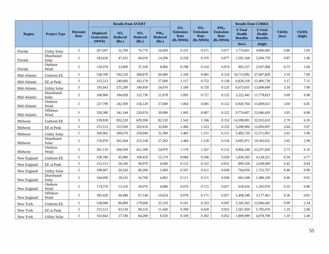
55


Rate


Emissions

Rate

(lb./MWh)

NOx

Emissions

Rate

(lb./MWh)

PM25

Emissions

Rate

(lb./MWh)

Results from COBRA

¢/kWh

(low) ¢/kWh

(high) Displaced

Generation

(MWh)

SO2

Reduced

(lbs.)

NOx

Reduced

(lbs.)

PM25

Reduced

(lbs.)

$ Total

Health

Benefits

$ Total

Health

Benefits

(low) (high)

Florida Utility Solar 3 207,097 52,790 76,770 16,050 0.255 0.371 0.077 1,774,601 4,006,685 0.86 1.93

Florida

Distributed

Solar 3 183,630 47,432 68,010 14,206 0.258 0.370 0.077 1,592,168 3,594,778 0.87 1.96

Florida

Onshore

Wind 3 120,474 23,900 37,320 8,860 0.198 0.310 0.074 902,527 2,037,968 0.75 1.69

Mid-Atlantic Uniform EE 3 538,700 592,310 368,870 66,980 1.100 0.685 0.124 16,713,992 37,697,828 3.10 7.00

Mid-Atlantic EE at Peak 3 215,513 240,660 162,170 27,600 1.117 0.752 0.128 6,828,318 15,400,738 3.17 7.15

Mid-Atlantic Utility Solar 3 195,643 215,290 140,850 24,470 1.100 0.720 0.125 6,073,655 13,698,689 3.10 7.00

Mid-Atlantic

Distributed

Solar 3 168,860 184,828 122,730 21,078 1.095 0.727 0.125 5,222,442 11,778,823 3.09 6.98

Mid-Atlantic

Onshore

Wind 3 227,799 242,300 156,120 27,840 1.064 0.685 0.122 6,920,764 15,609,621 3.04 6.85

Mid-Atlantic

Offshore

Wind 3 320,380 341,144 220,074 39,096 1.065 0.687 0.122 9,774,607 22,046,410 3.05 6.88

Midwest Uniform EE 3 539,830 832,220 629,590 82,120 1.542 1.166 0.152 14,598,081 32,932,610 2.70 6.10

Midwest EE at Peak 3 215,513 315,930 263,610 32,840 1.466 1.223 0.152 5,698,984 12,856,697 2.64 5.97

Midwest Utility Solar 3 206,962 306,670 250,640 31,300 1.482 1.211 0.151 5,483,726 12,371,091 2.65 5.98

Midwest

Distributed

Solar 3 176,970 262,564 215,538 27,292 1.484 1.218 0.154 4,695,971 10,593,932 2.65 5.99

Midwest

Onshore

Wind 3 361,110 566,930 421,590 54,970 1.570 1.167 0.152 9,866,248 22,257,830 2.73 6.16

New England Uniform EE 3 538,780 45,490 100,420 15,170 0.084 0.186 0.028 1,830,393 4,128,321 0.34 0.77

New England EE at Peak 3 215,513 26,540 49,970 6,640 0.123 0.232 0.031 899,328 2,028,969 0.42 0.94

New England Utility Solar 3 190,467 20,320 40,260 5,660 0.107 0.211 0.030 764,056 1,723,707 0.40 0.90

New England

Distributed

Solar 3 164,690 18,232 34,760 4,862 0.111 0.211 0.030 663,168 1,496,109 0.40 0.91

New England

Onshore

Wind 3 174,570 13,310 30,070 4,680 0.076 0.172 0.027 618,426 1,395,070 0.35 0.80

New England

Offshore

Wind 3 393,420 30,498 67,140 10,624 0.078 0.171 0.027 1,408,548 3,177,461 0.36 0.81

New York Uniform EE 3 538,680 86,890 179,600 25,510 0.161 0.333 0.047 5,345,565 12,046,445 0.99 2.24

New York EE at Peak 3 215,513 43,130 90,510 11,430 0.200 0.420 0.053 2,567,459 5,785,676 1.19 2.68

New York Utility Solar 3 163,842 27,740 64,280 8,550 0.169 0.392 0.052 1,809,989 4,078,700 1.10 2.49

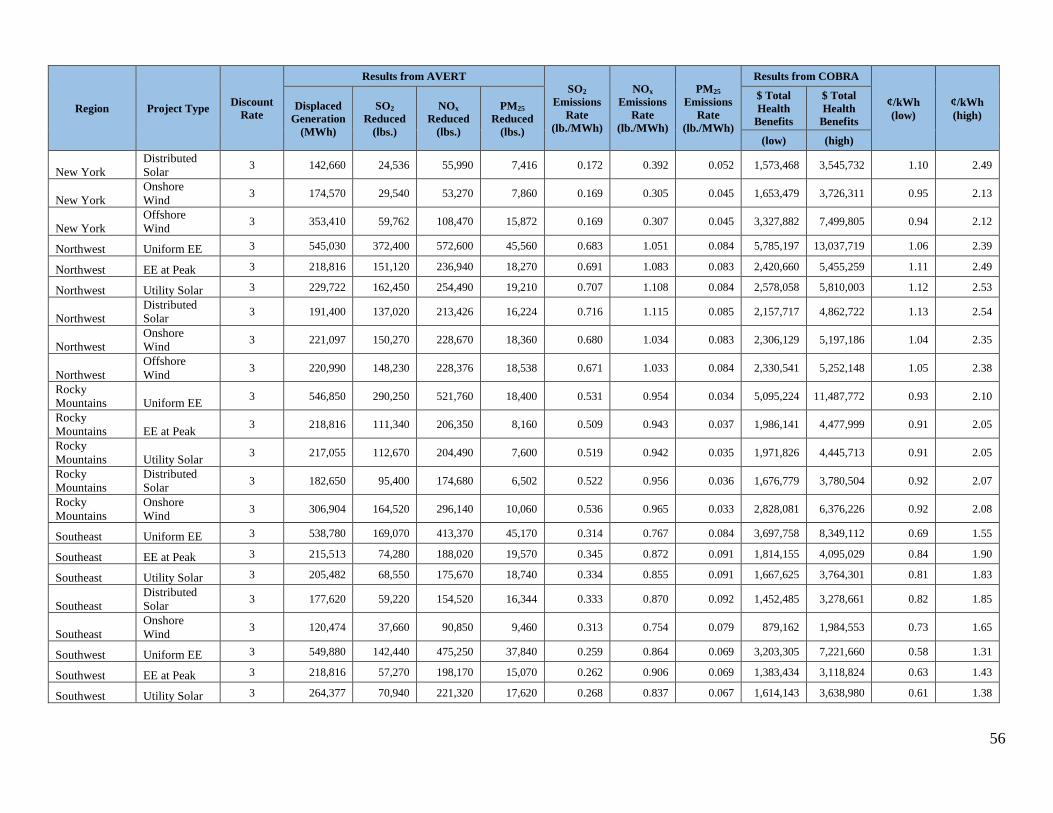
56


Rate


Emissions

Rate

(lb./MWh)

NOx

Emissions

Rate

(lb./MWh)

PM25

Emissions

Rate

(lb./MWh)

Results from COBRA

¢/kWh

(low) ¢/kWh

(high) Displaced

Generation

(MWh)

SO2

Reduced

(lbs.)

NOx

Reduced

(lbs.)

PM25

Reduced

(lbs.)

$ Total

Health

Benefits

$ Total

Health

Benefits

(low) (high)

New York

Distributed

Solar 3 142,660 24,536 55,990 7,416 0.172 0.392 0.052 1,573,468 3,545,732 1.10 2.49

New York

Onshore

Wind 3 174,570 29,540 53,270 7,860 0.169 0.305 0.045 1,653,479 3,726,311 0.95 2.13

New York

Offshore

Wind 3 353,410 59,762 108,470 15,872 0.169 0.307 0.045 3,327,882 7,499,805 0.94 2.12

Northwest Uniform EE 3 545,030 372,400 572,600 45,560 0.683 1.051 0.084 5,785,197 13,037,719 1.06 2.39

Northwest EE at Peak 3 218,816 151,120 236,940 18,270 0.691 1.083 0.083 2,420,660 5,455,259 1.11 2.49

Northwest Utility Solar 3 229,722 162,450 254,490 19,210 0.707 1.108 0.084 2,578,058 5,810,003 1.12 2.53

Northwest

Distributed

Solar 3 191,400 137,020 213,426 16,224 0.716 1.115 0.085 2,157,717 4,862,722 1.13 2.54

Northwest

Onshore

Wind 3 221,097 150,270 228,670 18,360 0.680 1.034 0.083 2,306,129 5,197,186 1.04 2.35

Northwest

Offshore

Wind 3 220,990 148,230 228,376 18,538 0.671 1.033 0.084 2,330,541 5,252,148 1.05 2.38

Rocky

Mountains Uniform EE 3 546,850 290,250 521,760 18,400 0.531 0.954 0.034 5,095,224 11,487,772 0.93 2.10

Rocky

Mountains EE at Peak 3 218,816 111,340 206,350 8,160 0.509 0.943 0.037 1,986,141 4,477,999 0.91 2.05

Rocky

Mountains Utility Solar 3 217,055 112,670 204,490 7,600 0.519 0.942 0.035 1,971,826 4,445,713 0.91 2.05

Rocky

Mountains

Distributed

Solar 3 182,650 95,400 174,680 6,502 0.522 0.956 0.036 1,676,779 3,780,504 0.92 2.07

Rocky

Mountains

Onshore

Wind 3 306,904 164,520 296,140 10,060 0.536 0.965 0.033 2,828,081 6,376,226 0.92 2.08

Southeast Uniform EE 3 538,780 169,070 413,370 45,170 0.314 0.767 0.084 3,697,758 8,349,112 0.69 1.55

Southeast EE at Peak 3 215,513 74,280 188,020 19,570 0.345 0.872 0.091 1,814,155 4,095,029 0.84 1.90

Southeast Utility Solar 3 205,482 68,550 175,670 18,740 0.334 0.855 0.091 1,667,625 3,764,301 0.81 1.83

Southeast

Distributed

Solar 3 177,620 59,220 154,520 16,344 0.333 0.870 0.092 1,452,485 3,278,661 0.82 1.85

Southeast

Onshore

Wind 3 120,474 37,660 90,850 9,460 0.313 0.754 0.079 879,162 1,984,553 0.73 1.65

Southwest Uniform EE 3 549,880 142,440 475,250 37,840 0.259 0.864 0.069 3,203,305 7,221,660 0.58 1.31

Southwest EE at Peak 3 218,816 57,270 198,170 15,070 0.262 0.906 0.069 1,383,434 3,118,824 0.63 1.43

Southwest Utility Solar 3 264,377 70,940 221,320 17,620 0.268 0.837 0.067 1,614,143 3,638,980 0.61 1.38

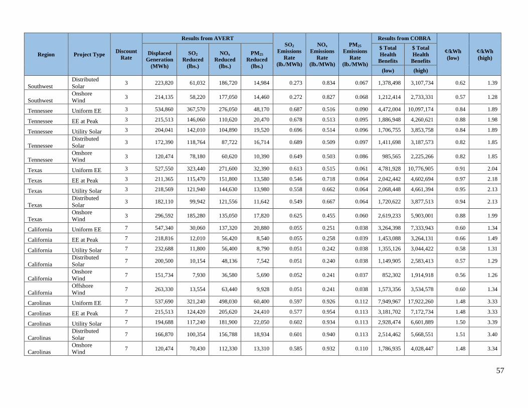
57


Rate


Emissions

Rate

(lb./MWh)

NOx

Emissions

Rate

(lb./MWh)

PM25

Emissions

Rate

(lb./MWh)

Results from COBRA

¢/kWh

(low) ¢/kWh

(high) Displaced

Generation

(MWh)

SO2

Reduced

(lbs.)

NOx

Reduced

(lbs.)

PM25

Reduced

(lbs.)

$ Total

Health

Benefits

$ Total

Health

Benefits

(low) (high)

Southwest

Distributed

Solar 3 223,820 61,032 186,720 14,984 0.273 0.834 0.067 1,378,498 3,107,734 0.62 1.39

Southwest

Onshore

Wind 3 214,135 58,220 177,050 14,460 0.272 0.827 0.068 1,212,414 2,733,331 0.57 1.28

Tennessee Uniform EE 3 534,860 367,570 276,050 48,170 0.687 0.516 0.090 4,472,004 10,097,174 0.84 1.89

Tennessee EE at Peak 3 215,513 146,060 110,620 20,470 0.678 0.513 0.095 1,886,948 4,260,621 0.88 1.98

Tennessee Utility Solar 3 204,041 142,010 104,890 19,520 0.696 0.514 0.096 1,706,755 3,853,758 0.84 1.89

Tennessee

Distributed

Solar 3 172,390 118,764 87,722 16,714 0.689 0.509 0.097 1,411,698 3,187,573 0.82 1.85

Tennessee

Onshore

Wind 3 120,474 78,180 60,620 10,390 0.649 0.503 0.086 985,565 2,225,266 0.82 1.85

Texas Uniform EE 3 527,550 323,440 271,600 32,390 0.613 0.515 0.061 4,781,928 10,776,905 0.91 2.04

Texas EE at Peak 3 211,365 115,470 151,800 13,580 0.546 0.718 0.064 2,042,442 4,602,694 0.97 2.18

Texas Utility Solar 3 218,569 121,940 144,630 13,980 0.558 0.662 0.064 2,068,448 4,661,394 0.95 2.13

Texas

Distributed

Solar 3 182,110 99,942 121,556 11,642 0.549 0.667 0.064 1,720,622 3,877,513 0.94 2.13

Texas

Onshore

Wind 3 296,592 185,280 135,050 17,820 0.625 0.455 0.060 2,619,233 5,903,001 0.88 1.99

California Uniform EE 7 547,340 30,060 137,320 20,880 0.055 0.251 0.038 3,264,398 7,333,943 0.60 1.34

California EE at Peak 7 218,816 12,010 56,420 8,540 0.055 0.258 0.039 1,453,088 3,264,131 0.66 1.49

California Utility Solar 7 232,688 11,800 56,400 8,790 0.051 0.242 0.038 1,355,126 3,044,422 0.58 1.31

California

Distributed

Solar 7 200,500 10,154 48,136 7,542 0.051 0.240 0.038 1,149,905 2,583,413 0.57 1.29

California

Onshore

Wind 7 151,734 7,930 36,580 5,690 0.052 0.241 0.037 852,302 1,914,918 0.56 1.26

California

Offshore

Wind 7 263,330 13,554 63,440 9,928 0.051 0.241 0.038 1,573,356 3,534,578 0.60 1.34

Carolinas Uniform EE 7 537,690 321,240 498,030 60,400 0.597 0.926 0.112 7,949,967 17,922,260 1.48 3.33

Carolinas EE at Peak 7 215,513 124,420 205,620 24,410 0.577 0.954 0.113 3,181,702 7,172,734 1.48 3.33

Carolinas Utility Solar 7 194,688 117,240 181,900 22,050 0.602 0.934 0.113 2,928,474 6,601,889 1.50 3.39

Carolinas

Distributed

Solar 7 166,870 100,354 156,788 18,934 0.601 0.940 0.113 2,514,462 5,668,551 1.51 3.40

Carolinas

Onshore

Wind 7 120,474 70,430 112,330 13,310 0.585 0.932 0.110 1,786,935 4,028,447 1.48 3.34

58


Rate


Emissions

Rate

(lb./MWh)

NOx

Emissions

Rate

(lb./MWh)

PM25

Emissions

Rate

(lb./MWh)

Results from COBRA

¢/kWh

(low) ¢/kWh

(high) Displaced

Generation

(MWh)

SO2

Reduced

(lbs.)

NOx

Reduced

(lbs.)

PM25

Reduced

(lbs.)

$ Total

Health

Benefits

$ Total

Health

Benefits

(low) (high)

Carolinas

Offshore

Wind 7 244,230 143,772 229,740 27,260 0.589 0.941 0.112 3,613,053 8,145,216 1.48 3.34

Central Uniform EE 7 539,450 678,890 642,870 42,000 1.258 1.192 0.078 6,580,497 14,827,027 1.22 2.75

Central EE at Peak 7 215,513 245,840 279,290 17,380 1.141 1.296 0.081 2,551,306 5,748,478 1.18 2.67

Central Utility Solar 7 225,810 266,470 284,790 17,860 1.180 1.261 0.079 2,692,585 6,066,833 1.19 2.69

Central

Distributed

Solar 7 190,820 225,580 242,526 15,160 1.182 1.271 0.079 2,284,457 5,147,252 1.20 2.70

Central

Onshore

Wind 7 351,609 458,062 412,528 27,292 1.303 1.173 0.078 4,372,416 9,851,863 1.24 2.80

Florida Uniform EE 7 538,270 115,180 176,720 40,370 0.214 0.328 0.075 3,765,548 8,498,776 0.70 1.58

Florida EE at Peak 7 215,513 60,190 84,860 16,980 0.279 0.394 0.079 1,748,146 3,944,964 0.81 1.83

Florida Utility Solar 7 207,097 52,790 76,770 16,050 0.255 0.371 0.077 1,583,663 3,573,994 0.76 1.73

Florida

Distributed

Solar 7 183,630 47,432 68,010 14,206 0.258 0.370 0.077 1,420,860 3,206,570 0.77 1.75

Florida

Onshore

Wind 7 120,474 23,900 37,320 8,860 0.198 0.310 0.074 805,422 1,817,909 0.67 1.51

Mid-Atlantic Uniform EE 7 538,700 592,310 368,870 66,980 1.100 0.685 0.124 14,955,407 33,711,920 2.78 6.26

Mid-Atlantic EE at Peak 7 215,513 240,660 162,170 27,600 1.117 0.752 0.128 6,093,791 13,736,140 2.83 6.37

Mid-Atlantic Utility Solar 7 195,643 215,290 140,850 24,470 1.100 0.720 0.125 5,420,312 12,218,060 2.77 6.25

Mid-Atlantic

Distributed

Solar 7 168,860 184,828 122,730 21,078 1.095 0.727 0.125 4,660,669 10,505,712 2.76 6.22

Mid-Atlantic

Onshore

Wind 7 227,799 242,300 156,120 27,840 1.064 0.685 0.122 6,176,257 13,922,389 2.71 6.11

Mid-Atlantic

Offshore

Wind 7 320,380 341,144 220,074 39,096 1.065 0.687 0.122 8,723,106 19,663,447 2.72 6.14

Midwest Uniform EE 7 539,830 832,220 629,590 82,120 1.542 1.166 0.152 13,004,100 29,319,058 2.41 5.43

Midwest EE at Peak 7 215,513 315,930 263,610 32,840 1.466 1.223 0.152 5,086,458 11,467,941 2.36 5.32

Midwest Utility Solar 7 206,962 306,670 250,640 31,300 1.482 1.211 0.151 4,894,341 11,034,794 2.36 5.33

Midwest

Distributed

Solar 7 176,970 262,564 215,538 27,292 1.484 1.218 0.154 4,191,255 9,449,600 2.37 5.34

Midwest

Onshore

Wind 7 361,110 566,930 421,590 54,970 1.570 1.167 0.152 8,805,831 19,853,606 2.44 5.50

New England Uniform EE 7 538,780 45,490 100,420 15,170 0.084 0.186 0.028 1,750,119 3,946,006 0.32 0.73

New England EE at Peak 7 215,513 26,540 49,970 6,640 0.123 0.232 0.031 802,531 1,809,651 0.37 0.84

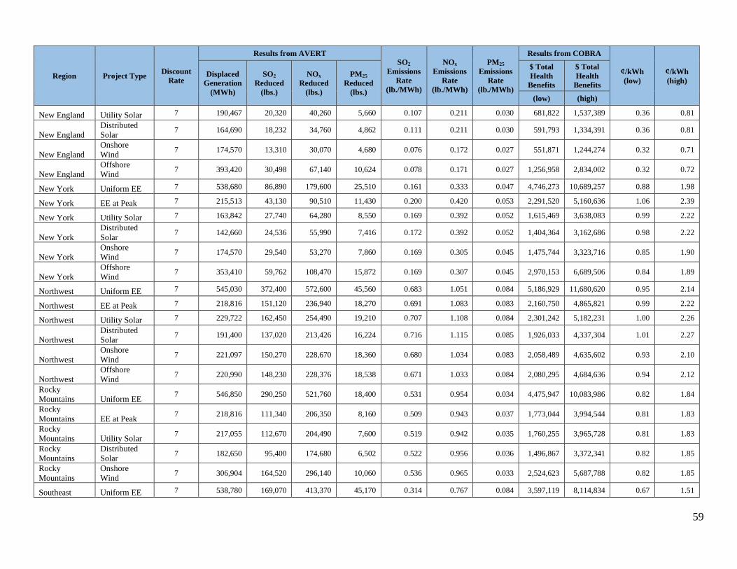
59


Rate


Emissions

Rate

(lb./MWh)

NOx

Emissions

Rate

(lb./MWh)

PM25

Emissions

Rate

(lb./MWh)

Results from COBRA

¢/kWh

(low) ¢/kWh

(high) Displaced

Generation

(MWh)

SO2

Reduced

(lbs.)

NOx

Reduced

(lbs.)

PM25

Reduced

(lbs.)

$ Total

Health

Benefits

$ Total

Health

Benefits

(low) (high)

New England Utility Solar 7 190,467 20,320 40,260 5,660 0.107 0.211 0.030 681,822 1,537,389 0.36 0.81

New England

Distributed

Solar 7 164,690 18,232 34,760 4,862 0.111 0.211 0.030 591,793 1,334,391 0.36 0.81

New England

Onshore

Wind 7 174,570 13,310 30,070 4,680 0.076 0.172 0.027 551,871 1,244,274 0.32 0.71

New England

Offshore

Wind 7 393,420 30,498 67,140 10,624 0.078 0.171 0.027 1,256,958 2,834,002 0.32 0.72

New York Uniform EE 7 538,680 86,890 179,600 25,510 0.161 0.333 0.047 4,746,273 10,689,257 0.88 1.98

New York EE at Peak 7 215,513 43,130 90,510 11,430 0.200 0.420 0.053 2,291,520 5,160,636 1.06 2.39

New York Utility Solar 7 163,842 27,740 64,280 8,550 0.169 0.392 0.052 1,615,469 3,638,083 0.99 2.22

New York

Distributed

Solar 7 142,660 24,536 55,990 7,416 0.172 0.392 0.052 1,404,364 3,162,686 0.98 2.22

New York

Onshore

Wind 7 174,570 29,540 53,270 7,860 0.169 0.305 0.045 1,475,744 3,323,716 0.85 1.90

New York

Offshore

Wind 7 353,410 59,762 108,470 15,872 0.169 0.307 0.045 2,970,153 6,689,506 0.84 1.89

Northwest Uniform EE 7 545,030 372,400 572,600 45,560 0.683 1.051 0.084 5,186,929 11,680,620 0.95 2.14

Northwest EE at Peak 7 218,816 151,120 236,940 18,270 0.691 1.083 0.083 2,160,750 4,865,821 0.99 2.22

Northwest Utility Solar 7 229,722 162,450 254,490 19,210 0.707 1.108 0.084 2,301,242 5,182,231 1.00 2.26

Northwest

Distributed

Solar 7 191,400 137,020 213,426 16,224 0.716 1.115 0.085 1,926,033 4,337,304 1.01 2.27

Northwest

Onshore

Wind 7 221,097 150,270 228,670 18,360 0.680 1.034 0.083 2,058,489 4,635,602 0.93 2.10

Northwest

Offshore

Wind 7 220,990 148,230 228,376 18,538 0.671 1.033 0.084 2,080,295 4,684,636 0.94 2.12

Rocky

Mountains Uniform EE 7 546,850 290,250 521,760 18,400 0.531 0.954 0.034 4,475,947 10,083,986 0.82 1.84

Rocky

Mountains EE at Peak 7 218,816 111,340 206,350 8,160 0.509 0.943 0.037 1,773,044 3,994,544 0.81 1.83

Rocky

Mountains Utility Solar 7 217,055 112,670 204,490 7,600 0.519 0.942 0.035 1,760,255 3,965,728 0.81 1.83

Rocky

Mountains

Distributed

Solar 7 182,650 95,400 174,680 6,502 0.522 0.956 0.036 1,496,867 3,372,341 0.82 1.85

Rocky

Mountains

Onshore

Wind 7 306,904 164,520 296,140 10,060 0.536 0.965 0.033 2,524,623 5,687,788 0.82 1.85

Southeast Uniform EE 7 538,780 169,070 413,370 45,170 0.314 0.767 0.084 3,597,119 8,114,834 0.67 1.51

60


Rate


Emissions

Rate

(lb./MWh)

NOx

Emissions

Rate

(lb./MWh)

PM25

Emissions

Rate

(lb./MWh)

Results from COBRA

¢/kWh

(low) ¢/kWh

(high) Displaced

Generation

(MWh)

SO2

Reduced

(lbs.)

NOx

Reduced

(lbs.)

PM25

Reduced

(lbs.)

$ Total

Health

Benefits

$ Total

Health

Benefits

(low) (high)

Southeast EE at Peak 7 215,513 74,280 188,020 19,570 0.345 0.872 0.091 1,619,303 3,652,964 0.75 1.70

Southeast Utility Solar 7 205,482 68,550 175,670 18,740 0.334 0.855 0.091 1,488,513 3,357,942 0.72 1.63

Southeast

Distributed

Solar 7 177,620 59,220 154,520 16,344 0.333 0.870 0.092 1,296,480 2,924,727 0.73 1.65

Southeast

Onshore

Wind 7 120,474 37,660 90,850 9,460 0.313 0.754 0.079 784,736 1,770,321 0.65 1.47

Southwest Uniform EE 7 549,880 142,440 475,250 37,840 0.259 0.864 0.069 2,838,081 6,393,353 0.52 1.16

Southwest EE at Peak 7 218,816 57,270 198,170 15,070 0.262 0.906 0.069 1,234,958 2,781,939 0.56 1.27

Southwest Utility Solar 7 264,377 70,940 221,320 17,620 0.268 0.837 0.067 1,440,895 3,245,902 0.55 1.23

Southwest

Distributed

Solar 7 223,820 61,032 186,720 14,984 0.273 0.834 0.067 1,230,542 2,772,041 0.55 1.24

Southwest

Onshore

Wind 7 214,135 58,220 177,050 14,460 0.272 0.827 0.068 1,082,276 2,438,076 0.51 1.14

Tennessee Uniform EE 7 534,860 367,570 276,050 48,170 0.687 0.516 0.090 4,018,966 9,069,390 0.75 1.70

Tennessee EE at Peak 7 215,513 146,060 110,620 20,470 0.678 0.513 0.095 1,684,171 3,800,728 0.78 1.76

Tennessee Utility Solar 7 204,041 142,010 104,890 19,520 0.696 0.514 0.096 1,523,345 3,437,785 0.75 1.68

Tennessee

Distributed

Solar 7 172,390 118,764 87,722 16,714 0.689 0.509 0.097 1,259,996 2,843,512 0.73 1.65

Tennessee

Onshore

Wind 7 120,474 78,180 60,620 10,390 0.649 0.503 0.086 879,656 1,985,066 0.73 1.65

Texas Uniform EE 7 527,550 323,440 271,600 32,390 0.613 0.515 0.061 4,277,976 9,632,974 0.81 1.83

Texas EE at Peak 7 211,365 115,470 151,800 13,580 0.546 0.718 0.064 1,823,735 4,106,268 0.86 1.94

Texas Utility Solar 7 218,569 121,940 144,630 13,980 0.558 0.662 0.064 1,846,940 4,158,622 0.85 1.90

Texas

Distributed

Solar 7 182,110 99,942 121,556 11,642 0.549 0.667 0.064 1,536,370 3,459,297 0.84 1.90

Texas

Onshore

Wind 7 296,592 185,280 135,050 17,820 0.625 0.455 0.060 2,338,672 5,266,235 0.79 1.78

61

Appendix H: Comparison Between 2017 and 2019 BPK Values There are five regions (California, Northwest, Rocky Mountains, Southwest, and Texas) that

have largely stayed the same between the two years, and which can enable a comparison.31

Table H-1 shows the 2017 and 2019 BPK values (low end, 3% discount rate) for these regions.

All regions except for California show a decrease in the BPK values between 2017 and 2019.

There are multiple factors that drive changes in BPK between years. First, in AVERT, the

electricity grid is generally getting cleaner, resulting in few emissions per megawatt-hour of

generation (Table H-2). This results in a reduction in BPK values, because EE/RE displacing

cleaner electricity produces less benefits.

A second factor impacting the BPK values is the population, which has increased in most areas,

according to data from the U.S. Census Bureau (2020). Higher populations result in higher

benefits (and therefore higher BPK values), because there are more people breathing cleaner air.

In most regions, the reduction in benefits due to reduced emission rates outweighs the increase in

benefits due to increased population. The net result of this is a decrease in BPK values between

2017 and 2019 for most regions.

California shows a net increase in BPK values because its emission rates did not change very

much between 2017 and 2019, and therefore the increase in population in California outweighed

the decrease in benefits from lower emission rates.

Table H-1. Comparison of 2017 and 2019 BPK Values for Select Regions

Region Technology

BPK Value (¢/kWh)

Low Value, 3%

Discount Rate

High Value, 3%

Discount Rate

Low Value, 7%

Discount Rate

High Value, 7%

Discount Rate

2017 2019 2017 2019 2017 2019 2017 2019

California EE at Peak 0.52 0.72 1.17 1.61 0.46 0.64 1.04 1.43

California Onshore Wind 0.48 0.60 1.09 1.36 0.43 0.54 0.97 1.21

California Uniform EE 0.48 0.64 1.08 1.45 0.42 0.57 0.96 1.29

California Utility Solar 0.51 0.63 1.15 1.41 0.45 0.56 1.03 1.26

Northwest EE at Peak 1.12 1.06 2.54 2.40 1.00 0.95 2.27 2.14

Northwest Onshore Wind 1.13 1.00 2.55 2.26 1.01 0.90 2.27 2.02

Northwest Uniform EE 1.13 1.02 2.55 2.30 1.01 0.92 2.28 2.06

Northwest Utility Solar 1.17 1.08 2.64 2.43 1.04 0.96 3.91 2.17

Rocky Mountains EE at Peak 0.98 0.87 2.21 1.97 0.87 0.78 1.98 1.76

Rocky Mountains Onshore Wind 1.07 0.89 2.41 2.00 0.95 0.79 2.15 1.78

Rocky Mountains Uniform EE 1.03 0.90 2.32 2.02 0.92 0.79 2.07 1.77

Rocky Mountains Utility Solar 0.99 0.87 2.25 1.97 0.89 0.78 2.01 1.76

31 Even though the borders of these regions are largely unchanged, there have been some changes in which

electricity generating units are assigned to which regions. Nevertheless, these regions remain the best regions for a

comparison between the 2017 and 2019 BPK values.

62

Region Technology

BPK Value (¢/kWh)

Low Value, 3%

Discount Rate

High Value, 3%

Discount Rate

Low Value, 7%

Discount Rate

High Value, 7%

Discount Rate

2017 2019 2017 2019 2017 2019 2017 2019

Southwest EE at Peak 0.70 0.61 1.59 1.37 0.63 0.54 1.42 1.22

Southwest Onshore Wind 0.77 0.54 1.73 1.23 0.68 0.49 1.54 1.09

Southwest Uniform EE 0.71 0.56 1.62 1.26 0.64 0.50 1.44 1.12

Southwest Utility Solar 0.73 0.59 1.73 1.32 0.65 0.52 1.46 1.18

Texas EE at Peak 1.39 0.93 3.13 2.09 1.24 0.83 2.80 1.87

Texas Onshore Wind 1.63 0.85 3.69 1.91 1.45 0.76 3.29 1.71

Texas Uniform EE 1.58 0.87 3.58 1.96 1.41 0.78 3.19 1.76

Texas Utility Solar 1.42 0.91 3.22 2.05 1.27 0.81 2.87 1.83

Table H-2. Comparison of 2017 and 2019 BPK Values for Select Regions

Region Pollutant

Emission Rates

(lbs./MWh) %

Difference 2017 2019

California NOx 0.34 0.30 -12%

Northwest NOx 1.29 1.09 -16%

Rocky Mountains NOx 1.42 1.08 -24%

Southwest NOx 0.99 0.88 -11%

Texas NOx 0.65 0.51 -22%

California SO2 0.08 0.06 -27%

Northwest SO2 0.92 0.72 -22%

Rocky Mountains SO2 0.60 0.71 17%

Southwest SO2 0.24 0.34 38%

Texas SO2 1.32 0.86 -35%

California PM2.5 0.05 0.04 -11%

Northwest PM2.5 0.09 0.08 -5%

Rocky Mountains PM2.5 0.04 0.03 -15%

Southwest PM2.5 0.08 0.08 10%

Texas PM2.5 0.08 0.07 -12%

63

Appendix I: Conversions Table I–1 lists common conversions used throughout this report.

Table I-1. Common Conversions

Original Units Multiply by To Obtain

¢/kWh 1,000 ¢/MWh

¢/kWh 1,000,000 ¢/GWh

64

U.S. Environmental Protection Agency State and Local Climate and Energy Program 1200 Pennsylvania Ave, NW (6202A) Washington, DC 20460 452R21001 epa.gov/statelocalenergy May 2021