Embed Size (px)
Citation preview

LSM -28Li5liS APRIL 1987
Living StancdarcdsMleasurement SfuJx1vVorking Paper- \ '
Analysis of Household Expenditures
Ang'* A,-0
Pub
lic D
iscl
osur
e A
utho
rized
Pub
lic D
iscl
osur
e A
utho
rized
Pub
lic D
iscl
osur
e A
utho
rized
Pub
lic D
iscl
osur
e A
utho
rized

LSMS WORKING PAPER SERIES
No. 1. Living Standards Surveys in Developing Countries.
No. 2. Poverty and Living Standards in Asia: An Overview of the Main Resultsand Lessons of Selected Household Surveys.
No. 3. Measuring Levels of Living in Latin America: An Overview of MainProblems.
No. 4. Towards More Effective Measurement of Levels of Living", and "Reviewof Work of the United Nations Statistical Office (UNSO) Related toStatistics of Levels of Living.
No. 5. Conducting Surveys in Developing Countries: Practical Problems andExperience in Brazil, Malaysia, and the Philippines.
No. 6. Household Survey Experience in Africa.
No. 7. Measurement of Welfare: Theory and Practical Guidelines.
No. 8. Employment Data for the Measurement of Living Standards.
No. 9. Income and Expenditure Surveys in Developing Countries: Sample Designand Execution.
No. 10. Reflections on the LSMS Group Meeting.
No. 11. Three Essays on a Sri Lanka Household Survey.
No. 12. The ECIEL Study of Household Income and Consumption in Urban LatinAmerica: An Analytical History.
No. 13. Nutrition and Health Status Indicators: Suggestions for Surveys of theStandard of Living in Developing Countries.
No. 14. Child Schooling and the Measurement of Living Standards.
No. 15. Measuring Health as a Component of Living Standards.
No. 16. Procedures for Collecting and Analyzing Mortality Data in LSMS.
No. 17. The Labor Market and Social Accounting: A Framework of DataPresentation.
(List continues on the inside of the back cover)
LSMS Working PaperNumber 28
ANALYSIS OF HOUSEHOLD EXPENDITURES
Angus Deaton- andAnne Case
Development Research DepartmentThe World Bank
Washington, D.C. 20433, U.S.A.

This is a working document published informally by the Development
Research Department of The World Bank. The World Bank does not accept
responsiblity for the views expressed herein, which are those of the authors
and should not be attributed to the World Bank or to its affiliated
organizations. The findings, interpretations, and conclusions are the results
of research supported by the Bank; they do not necessarily represent official
policy of the Bank. The designations employed, the presentation of materials,
and any maps used in this document are solely for the convenience of the
reader and do not imply the expression of any opinion whatsoever on the part
of the World Bank or its affiliates concerning the legal status of any
country, territory, city, area, or of its authorities, or concerning the
delimitation of its boundaries, or national affiliation.
The LSMS working paper series may be obtained from the Living
Standards Measurement Study, Development Research Department, The World Bank,
1818 H Street, N.W., Washington, D.C. 20433, U.S.A.
Angus Deaton is a consultant to the Living Standards Unit, The World
Bank and is William Church Osborn Professor of Public Affairs and Professor of
Economics and International Affairs, Woodrow Wilson School and Department of
Economics, Princeton University. Anne Case is Research Assistant to Angus
Deaton at Woodrow Wilson School, Princeton University.
April 1987
- iii-
PREFACE
The Living Standards Measurement Study (LSMS) was established by the
World Bank in 1980 to explore ways of improving the type and quality of
household data collected by Third World statistical offices. Its goal is to
foster increased use of household data as a basis for policy decision
making. Specifically, the LSMS is working to develop new methods to monitor
progress in raising levels of living, to identify the consequences for
households of past and proposed government policies, and to improve
communications between survey statisticians, analysts, and policy makers.
The LSMS Working Paper series was started to disseminate
intermediate products from the LSMS. Publications in the series include
critical surveys covering different aspects of the LSMS data collection
program; reports on improved methodologies for using Living Standards Survey
(LSS) data; and recommendations on specific survey, questionnaire and data
processing designs. Future publications will demonstrate the breadth of
policy analysis that can be carried out using LSS data.

- iv -
ACKNOWLEDGMENTS
The authors are grateful to Dennis de Tray and Jacques van der Gaag
of the Living Standards Unit, and to John Muellbauer, Nuffield College, Oxford
for their comments on an earlier version. Margaret Irish (University of
Bristol) and Duncan Thomas (Princeton University) provided help with the
computations.

v
ABSTRACT
In any society, one of the ultimate objectives of the economic system
is to deliver goods and services to its members. The success of an economy
can be measured by its ability to provide for its people, to feed them, to
clothe and shelter them, and to offer them access to good health, to education
and to a wide range of consumer goods. The household expenditure survey is
the tool through which material welfare is measured. Its results inform about
levels of living, about how these levels change over time, and about how
levels of living vary among individuals and groups in the economy. Beyond
this point, the wealth of data from such surveys provides an information base
that, in the short run, is an essential prerequisite for the evaluation of
actual or proposed policies and, in the long run, by enhancing our
understanding of how the economy functions, allows the evolution of better
policies for progress and development.
Using household expenditure surveys, we can explore a wide range of
issues that are both of substantive interest in their own right, and that help
improve our understanding of the functioning of the economy. In this paper,
we devote space to three such analytical issues; the estimation of Engel
curves, that is, the relationship between demand patterns, household budgets,
and their demographic composition; the calculation of measures of the costs of
maintaining children; and the calculation of price indices.

- vi -
TABLE OF CONTENTS
ACKNOWLEDGMENTS
ABSTRACT
Chapter I WHY MEASURE AND STUDY HOUSEHOLD EXPENDITURES? ..... 1Household Surveys and Living Standards .......... ISurveys as a Data Base for Policy Analysis ...... 4Surveys as a Data Base for Research ............. 9Notes for Further Reading ...................... 20
Chapter II A FRAMEWORK FOR DESCRIPTION ....................... 22Concepts ............................. 22Illustrative Numbers from Three Surveys .25Notes for Further Reading .43
Chapter III THE ESTIMATION OF ENGEL CURVES .44Food Shares and Total Expenditure .45Engel Curves for the Three Surveys .48Engel Curves and Household Composition .57Empirical Results for Three Surveys .64Notes for Further Reading .77
Chapter IV MEASURING THE COSTS OF CHILDREN .................. 80General Considerations ......................... 80Engel's Procedure ............................... 84Rothbarth's Method ............................. 86An Empirical Illustration ...................... 88Notes for Further Reading ...................... 97
Chapter V PRICES AND WELFARE ..... 99Aggregate Price Indices ........................ 99Disaggregated Price Indices ................... 102Prices, Profits and Consumer Surplus .......... 105Designing Taxes and Tax Reform ................ 110Notes for Further Reading ..................... 115
REFERENCES .. ..... 116
Table 2.1 The Disposition of Income and Expenditure:Sri Lanka 1969-70 . .................... 27
Table 2.2 The Disposition of Income and Expenditure:Sri Lanka 1980-81 .28
Table 2.3 The Disposition of Income and Expenditure:Indonesia 1978... . ....... . 29
Table 2.4 Proportions of the Food Budget Allocated toDifferent Food Groups: Indonesia 1978 .......... 36
Table 2.5 Expenditure to Income Ratios: Four Surveys ....... 38

-vii -
Table 2.6 A Comparison of Expenditure by PCE Decile:Sri Lanka 1969-70 and 1980-81 .................... 40
Table 3.1 $-Coefficients, Standard Errors, andExpenditure Elasticities: Sri Lanka 1969-70....49
Table 3.2 8-Coefficients, Standard Errors, andExpenditure Elasticities: Sri Lanka 1980-81....50
Table 3.3 8-Coefficients, Standard Errors, andExpenditure Elasticities: Indonesia 1978 ....... 51
Table 3.4 Adult and Child Composition of Sri LankanHouseholds by Sector .................... . 58
Table 3.5 Quadratic Regressions with Minimal DemographicEffects: Sri Lanka 1969-70 . .................... 68
Table 3.6 Quadratic Regressions with Minimal DemographicEffects: Sri Lanka 1980-81 . .................... 74
Table 3.7 Quadratic Regressions with Minimal DemographicEffects: Indonesia 1978 . ...................... 76
Table 4.1 Commodity Shares as a Percentage of TotalExpenditure and Fractions of HouseholdsPurchasing ........ 89
Table 4.2 Demographic Effects in Relation toIncome Effects on Demand ....................... 92
Table 4.3 Income Equivalents of an Additional ChildRelative to Per Capita Expenditure ............. 95
Table 5.1 Price Indices by Decile for HypotheticalPrice Change: Sri Lanka 1969-70 ............... 103
Table 5.2 Farm-Size and Proportion of Net ProducersPaddy-Farmers: Thailand 1975-76 .108
Figure 2.1 Share of Expenditure on Travel and lnPCE:Indonesia 1978 .34
Figure 2.2 Expenditure Shares by PCE Decile:Indonesia 1978 .42
Figure 3.1 Food Share and PCE: Sri Lanka 1969-70. 47Figure 3.2 Food Share and PCE: Indonesia 1978 .47Figure 3.3 Food Share: Indonesia 1978. 57Figure 3.4 Food Share and ln(PCE) for Selected Urban
Javanese types ..... 60Figure 3.5 Necessities and Luxuries: A Comparison of
Budget Shares, Urban Outer Islands,Indonesia 1978 . ...... .. .............. 69

CHAPTER I
WHY MEASURE AND STUDY HOUSEHOLD EXPENDITURES?
In any society, one of the ultimate objectives of the economic system
is to deliver goods and services to its members. The success of an economy
can be measured by its ability to provide for its people, to feed them, to
clothe and shelter them, and to offer them access to good health, to education
and to a wide range of consumer goods. On such things depends the material
welfare of individuals, so that to measure material welfare, we must measure
what and how much individuals consume. The household expenditure survey is
the tool through which such measurement is done. Its results inform about
levels of living, about how these levels change over time, and about how
levels of living vary among individuals and groups in the economy. Beyond
this, the wealth of data from such surveys provides an information base that,
in the short run, is an essential prerequisite for the evaluation of actual or
proposed policies and, in the longer run, by enhancing our understanding of
how the economy functions, allows the evolution of better policies for
progress and development.
In this introductory chapter, we expand on these themes in
preparation for the more detailed illustrations in the later chapters.
Household Surveys and Living Standards
The LSMS household budget survey is a component of the overall LSS
household survey that is described in detail elsewhere. The household

-2-
expenditures section of the survey is designed to provide a representative
picture over a country as a whole of living standards and of the consumption
levels of various goods. The randomness of the survey design is of crucial
importance in guaranteeing that the households included are representative.
It also ensures that quite small samples relative to the total population
(usually about I in 5000) are sufficient to give an accurate guide as to what
is happening in the country as a whole. In gathering the information, the
survey is not designed to estimate a single quantity, but rather to provide
data on a whole range of important indicators of living standards. Prime
amongst these is a measure of total household consumption or command over
resources. Within the LSMS framework, this is the central indicator of
material welfare, though as will be emphasized later, it must be interpreted
in conjunction with other data. Total consumption consists not only of goods
and services purchased by households, but also those that they produce and
consume themselves, as well as those important items (such as education and
health facilities) that are frequently provided at least in part on a communal
basis. The elements of household consumption are also of interest in their
own right. Patterns of consumption within the budget are important
determinants of the structure of economic activity, while the amounts consumed
of various goods, particularly foodstuffs, are among the determinants of
nutritional status, of health and of life-expectancy.
Two other elements of the survey should also be noted. Because it
covers the country as a whole, it provides data on the variation of
consumption patterns and expenditures across regions and over groups of
individuals. Efficient survey design in most developing countries requires
that the sample is broken up into separate regional or urban versus rural
-3-
surveys, each with its own sampling proportions, so that a natural output of
the survey is a corresponding regional breakdown of results. Even when not
built into the design, samples are usually large enough and representative
enough to allow breakdowns by other groups, for example, by occupational or
employment status. The value of such results is further enhanced if the
second element is incorporated, that is if the survey is repeated, if not
annually, at least at fairly regular intervals. Comparison of results between
surveys then permits an assessment of the evolution of living standards over
time, both in aggregate, and for specific groups of interest. Two household
surveys on a consistent basis but at different dates have an informational
value much greater than twice that of a single survey.
Once the data from the survey have been collected and processed, the
first results typically take the form of a published report containing tables
of the main variables of interest. These provide a compact description in a
fairly standard form of household living standards and consumption patterns at
the time of survey. We give examples of such descriptions in Chapter II. The
principal tables consist of estimates of total household expenditure and of
its components, often in some detail. Means for the population as a whole are
estimated, as are meanis for various subgroups distinguished (among other
things) by region, by occupation, by income and by family composition. Such
figures paint the broad outlines of who gets what and fulfill what has
traditionally been the most important role of household budget data, to
highlight the living conditions of the poor and to contrast them with those of
the rich, or at least with those of the moderately well-off administrators and
politicians at whom the survey results are aimed. Indeed, the earliest
household surveys in 18th and 19th century Europe were conceived with exactly
- 4 -
this purpose in mind, to document the poverty in which most households lived,
to overcome ignorance of this poverty by those in power, and to agitate for
social reform. For many countries even today, household surveys retain an
important role in providing information on distribution and poverty that
otherwise would be either unavailable or too easily and conveniently
ignored. Of course, even at a descriptive level, the data have many other
uses. The consumption totals are an important supplementary source and cross-
check for the national accounts. The pattern of demand, as represented by the
shares of each expenditure in the total, can be compared both across countries
and across time and, since we know a great deal about how these patterns
change historically and with economic development, any given set of shares
provides useful indicators of development. Expenditure shares also have the
advantage of being dimensionless and thus are free of at least some of the
measurement problems inherent in comparisons of, for example, per capita GDP
in U.S. dollars.
Surveys as a Data Base for Policy Analysis
However valuable the survey report with its tables and cross-
tabulations, it by no means exhausts the usefulness of the expenditure survey
as a data base. Indeed, if the survey report is the only use ever made of the
survey material, then the survey has only yielded a very small fraction of the
total possible return to the resources used to set it up. Unfortunately, this
sort of waste of resources is very common in practice, and one of the major
aims of the LSMS is to encourage the full and efficient use of survey results
primarily in policy making and secondarily in research. In a typical
household survey, some ten thousand households are interviewed, and each may

-5-
provide quantitative or qualitative responses to several hundred questions.
The original data set therefore contains between one and ten million separate
numbers. Of course much of this information, even if accurate, is essentially
irrelevant; the largely random variations in behaviour from one individual to
the next are of little or no interest either for description or the conduct of
policy. But these millions of numbers can be thought of as delineating the
empirical joint distribution of hundreds of variables, only a tiny fraction of
which is represented in the one-way, two-way or three-way cross-tabulations
that can appear in any report, however well-designed. In consequence, the
informational requirements of day-to-day policy evaluation and discussion,
even if met by the survey, may well not be met by the published report except
in the unlikely event of the report just happening to contain the precise
tabulation required.
We shall discuss examples of policy needs in several of the later
chapters and summarize some of the most important below, but it is clear that
the full exploitation of survey results requires that the full data set must
be maintained in a readily accessible form even after the first reports have
been published. New cross-tabulations should be obtainable very fast and at
low cost. These are not heavy demands in terms of modern computing and yet
the conditions for fulfilling them do not exist in a large number of
countries. Hopefully, the rapidly falling real cost of computing throughout
the world will soon remove such bottlenecks. But it is only when they are
removed that household surveys will yield the returns of which they are
capable.
What, then, are the policies for which household expenditure data are
so useful? The most obvious is the direction of aid, both inter- and intra-

-6-
nationally, where cash transfers are influenced by measures of poverty, most
usually by fairly crude figures such as the fraction of the population below
the poverty line. Household budget surveys are the source both for the
poverty line itself and for the counts of individuals below it. But even
without any formal link between aid and poverty, virtually all policy-making
in poor countries is carried out with the consequences for the poor born
heavily in mind, so that knowledge of who are the poor, where they are
located, and what they do to earn such support as they have, are indispensable
ingredients in any intelligent policy discussion. It is also generally
understood that the definition of poverty is a matter of great difficulty:
should it be based on food? On total expenditure? On nutritional or health
status? And if either of the former, how should we account for the differing
needs of children and (perhaps) of women? We shall address some of these
issues in Chapter IV below, but the very presence of this uncertainty
underlines the necessity of being able to take alternative approaches. Policy
makers must be able to make alternative definitions of poverty and to explore
the consequences of them for the incidence of "poverty" and the consequent
targeting of policy. Once again, this can only be done if the basic data are
readily available for the alternative calculations to be carried out quickly.
Household expenditure information is also indispensable in a second
major policy area, that of pricing, taxation and subsidy policy. In many
developing countries, it is difficult to collect income taxes except from a
rather small fraction of the population (those who work for the government or
elsewhere in the formal sector), so that indirect taxation (including pricing
policy and taxes on imports and exports) becomes the main instrument for
raising revenue and for meeting distributional objectives. Subsidies of
-7-
various forms are also typically important especially for food where
governments see the various schemes that exist as a means of guaranteeing
access to basic foods for the poor. Without household expenditure surveys, it
is impossible to assess even the immediate effects of such policies. However,
even minimal expenditure data can take us a long way. If we know how much is
consumed in aggregate together with some idea of response elasticity, we have
a first round estimate of the revenue that will be raised or lost by a tax
change. Just as important, if we know who consumes what, we can tell whose
welfare is affected by the tax change and, within an approximation, by how
much. For example, if the demand for a good tends to rise with income, or to
be confined to certain regions, then increasing the tax on it will be
progressive or will discriminate against those regions as the case may be.
Similarly, for food subsidy and distribution schemes, household expenditure
data tell us where the needs are located and thus how such schemes can be
designed so as to best serve those they are intended to help. To date,
household survey data have been less used in this respect than in the
measurement of poverty. However, it is also clear that many developing (and
many developed) countries have tax and subsidy systems that are the more or
less random result of the accretion of many different schemes each introduced
on a piecemeal basis. Systematic reconsideration of existing structures in
the light of their distributional and revenue consequences is an exercise that
is likely to have very large beneficial consequences at potentially very low
cost and it is an exercise that is impossible without good household budget
data. These issues are discussed at somewhat greater length in Chapter V
below.

-8-
There are many other good examples of the link between survey data
and policy but we mention here only one more. This is the part played by
household expenditure data in plannihg. Few developing countries leave the
structure of industry, employment and output entirely to determination by
market forces, although the degree of central direction varies enormously from
country to country. But whether the government is merely monitoring
development or actively planning it, a central question is how the structure
of the economy will or should develop over time. Planners must know which
industries and areas of employment will expand relatively and which will
contract. They must plan agricultural output and investment and set pricing
policies and procurement schemes so that, at least on average, the demand for
food can be met. Imports and exports of specific goods must be allowed for
and, in many countries this means setting quotas and planning foreign exchange
availability. In all of this, a central element is the structure of final
demand, its location, how it develops with changes in income and with the
distribution of that income between individuals and socioeconomic groups.
Again, household budget data can provide much relevant information. The
development of demand patterns across households as income varies can give
guidance (although not, unfortunately, solid predictions) as to what will
happen as income varies in the future. Similarly, information on the demand
patterns of particular groups enables an assessment of future changes in
demand as the relative importance and earning power of such groups changes
over time.

-9-
Surveys as a Data Base for Research
All the uses of the data discussed so far require little more than
cross-tabulation and inspection. If we go beyond this to a more analytical
treatment, it is possible to explore a wide range of issues that are both of
substantive interest in their own right, and that help improve our
understanding of the functioning of the economy. In this working paper, we
devote space to three such analytical issues; the estimation of Engel curves,
that is, the relationships between demand patterns, household budgets, and
their demographic composition; the calculation of measures of the costs of
maintaining children; and the calculation of price indices. The remainder of
this introduction contains a brief discussion of each of these topics and
explains why we believe that they are important enough to single out for
illustration in this study. Note however that, by focussing on these areas,
we do not seek to underplay the importance of other topics for analysis. In
practice, different questions will have different urgencies in different
countries. However, we expect that the three topics dealt with here will be
of general interest.
Engel curves are a systematic way of summarizing and describing the
development of consumption patterns as material resources increase. Hence,
the derivation and estimation of Engel curves is the obvious next step in the
analysis after the cross-tabulations have been drawn up. An explicit
mathematical relationship between demands and household resources allows us to
be more precise about the policy analyses discussed in the foregoing
paragraphs. Consider again the welfare effects of a price increase. It can
be shown that, to a first approximation, the elasticity of a given household's
cost-of-living with respect to the price change is given by the share in the

- 10 -
household's budget taken up by that commodity. Hence, if we view each Engel
curve as defining the relationship between the budget share and total
household expenditure (and this is the view that we shall formalize below),
then the Engel curve for a good delineates the distributional effects of a
change in its price.
Planning is another case where estimated Engel curves are useful.
Explicit mathematical forms are required for insertion into formal planning
models and provide the vital link between generated income and the pattern of
demand and thence to the structure of industrial and agricultural output and
finally back to employment and incomes. Such applications effectively assume
that Engel curves estimated from household surveys can be validly used to
project demands over time. Given the lack of alternative sources for demand
equations, such an assumption is probably inevitable. Nevertheless, it must
be treated with caution. By its nature, a cross-section as revealed by a
household survey compares different households at different income levels and
one cannot be certain of the differences in behavior of the same households at
different income levels. For example, behavior may be conditioned by relative
as well as by absolute incomes, so that proportional changes in all incomes,
as might occur with general economic growth, might well leave average demand
patterns approximately constant, even though in any given cross-section,
demand patterns are quite different at different income levels. Similar
phenomena also operate across countries as the tastes and technology that
accompany economic growth in the more developed countries are only partially
transmitted to their less developed neighbors. At the level of the raw data,
there are clear and major inconsistencies between cross-sectional, time-
series, and cross-country Engel curves. At a technical level, the problem is
- 11 -
one of inadequate conditioning; income in a time series has apparently
different effects from income in a cross-section because different things are
being (implicitly) held constant in the two experiments. If we could document
these other effects, and take them into account, the two measures of the
income effects would come together and it would be safe to predict using Engel
curves. In practice, prediction is easier and safer the more household
surveys that are available since, with suitable corrections, it is possible to
use each survey to check out the predictions made with the aid of its
predecessor.
Much of the literature on Engel curve analysis in developing
countries, and there is a great deal of it, has been concerned with a search
for the "best" function representing the curves. The scope and method of this
work is typically limited by the unavailability of the individual household
data, so that researchers must work with means of arbitrarily defined cells
thus losing important information that was available in the original survey.
With the individual data, the straightjacket is removed and it is possible to
work with models that are simultaneously both simpler and more powerful. In
Chapter III below we illustrate how this can be done.
Engel curve analysis is the starting point for our other illustrative
topics. The presence of children in the household clearly affects its demand
pattern and so must be taken into account if demands are to be understood and
predicted. At the same time, the alterations that children bring to household
consumption have traditionally been the basis for attempts to estimate the
costs of their upkeep. Taking the positive question first, demographic
variables or "household composition", as represented by the numbers of people
in the household, their age and sex, are the principal explanatory variables,
- 12 -
along with income, in explaining demand patterns in cross-section analysis.
Although income (or total outlay) is usually the dominant variable in the
explanation, it is clearly necessary that some attention must be given to at
least the number of people who share that income. Common observation suggests
that consumption needs and patterns shift with age and sex so that even
households with the same income and of the same size will not generally have
the same consumption patterns if their demographic compositions are
different. And even if we are primarily interested in the effects of income,
for example to establish demand equations for use in forecasting, then it is
still necessary to allow for the demographic effects if the influence of
income is to be accurately measured. To take a (perhaps) over-simplified
example, the budget shares might be put into a regression against (say) the
logarithm of total household expenditure instead of per capita household
expenditure. Since, over any given cross-section, family size is positively
correlated with total family expenditure, the expenditure elasticities will be
biased towards unity, that is, downwards for luxury goods and upwards for
necessities. In practice, no one is likely to ignore family size quite so
completely, but the point remains that, even in order to estimate income
elasticities, the demographic effects must be taken into account.
But, of course, the demographic effects are of major interest in
their own right and their estimation has just as much claim on our attention
as does that of income elasticities. The methodology we suggest in Chapter
III is designed to produce, from a first pass through the data, some
indication of the main "stylized facts" of household composition on demand
patterns. A wide range of important research topics depends, at least in
part, on the knowledge of these facts. We describe some of these topics

- 13 -
below, but the current point is not to lay out research programs to resolve
these issues but to generate data that cast light upon them. The first stage
of demand analysis is essentially exploratory, to discover what, if anything,
each data set can say about the effects of children, sex and age on
expenditure patterns.
We have already emphasized the importance of budget shares for
analyzing the effects of economic policy on individual welfare and hence how
the knowledge of variations in budget shares with income is essential for the
analysis of the distributional effects of economic policy. The same argument
holds for the relationship between household composition and the budget
shares. If food shares are higher for households with a large proportion of
children, then food price increases will bear disproportionately on such
households and hence on children themselves. At a more disaggregated level,
the association of particular commodity purchases with particular demographic
groups alerts us to the welfare impact of specific price changes. The same
also holds for sales. Groups whose livelihood depends on selling one
commodity to buy others can be forced into poverty and even starvation by
relative price changes if the price of what they sell falls and the price of
what they buy rises.
The effects of children on expenditure is also at the center of
attempts to measure the "costs" of children. Estimating such costs is
important for answering at least two important questions: how should we make
welfare comparisons between households with different numbers of members and
with different compositions? And what effects, if any, does the cost of

- 14 -
children have on fertility? We look briefly at each of these, if only to
highlight the relationship between these major issues and the empirical
analysis described later in the volume.
It is a well-known fact that in most household surveys, total
household expenditure is positively associated with household size. However,
as household size increases, total outlay rises less than in proportion so
that if we look not at total household expenditure, but at per capita
household expenditure, the latter is negatively correlated with household
size. Now, apart from fairly minor modifications, most studies choose either
total household expenditure or per capita household expenditure as a measure
of economic status and as the basis for inequality measurement. If the total
is chosen, then inevitably it is "discovered" that one of the major associates
of poverty (and from there it is not far to "cause") is small family size.
Other investigators, who choose per capita expenditure find that poverty is
typically associated with large family size. And, of course, there is little
difficulty in constructing "theories" of why either finding should be true.
The question naturally arises as to whether it is not possible to do better
than this by deriving some measure of the economic costs of children and
additional adults that is derived from measurement rather than from
assumption.
The task often appears straightforward. We observe small families
and we observe large families and surely the difference in their outlays must
be some measure of the costs of the extra indiviauals? The problem is that
such a procedure takes no account of the overall economic position of the two
families; the small family might be that of a rich businessman and the large
that of a poor farmer, so that the difference in their outlays is only very
- 15-
partially explained by their different compositions. One might be tempted to
restrict the comparisons to households with the same income, but this would
not really do either. If incomes are the same, then so must the total of
outlays be, at least if saving is included. And if saving is ignored, we are
effectively assuming that household composition has no effect on the timing of
consumption. The truth is that, given income, different household
compositions induce different patterns of demand within the same total outlay;
the birth of an extra child does nothing to complement household income but
rather causes a rearrangement of purchases, and possibly also of labor supply.
What is required is some rule or criterion which tells us when two
households with different compositions have the same welfare, so that
comparisons of outlays between such households, so called "equivalence
scales", are legitimate measures of the costs associated with the differing
compositions. Establishing such a criterion is no easy matter, and the
literature on child costs, although containing a number of suggestions,
contains no fully satisfactory non-controversial solution. For example, the
widely-used Engel methodology is based on the assumption that households with
the same share of food in total outlay are at the same welfare level. Some
people find this at least superficially plausible, but it is hard to tell a
convincing theoretical story which produces such a result, and the child costs
calculated using the method are typically far too large. In Chapter IV of
this study, we propose a different method for calculating child costs. Like
the Engel method, it is based on consumption of food and it is trivially easy
to calculate. However, unlike the Engel method, its assumptions are easier to
justify, and its estimates of child costs, at around one third of adult costs,
are much more plausible.

- 16 -
The relationship between child costs and fertility is another major
reason for being interested in demographic effects on demand patterns, though
the issues involved are different from those arising in estimating equivalence
scales. Equivalence scales have a wider scope since they attempt to summarize
the costs of household composition in general, not just of children. We want
to know how much less children consume, but also whether or not there are
significant economies of scale to several adults living in the same
households. When we move to questions of fertility, we are more narrowly
concerned with the costs of children, but at the same time the concepts of
costs (and benefits) are greatly extended.
Equivalence scales, if they measure anything at all, measure the
fairly short-run economic costs associated with the maintenance of and
provision for children. Such costs are an important element in fertility
decisions, but other long-term and less tangible costs and benefits are often
assigned a larger role. For example, much attention is given to the
importance of children as old-age insurance for their parents, or as "assets"
which spread risk against misfortune, or as means of gaining access to the
opportunities available in rapidly developing urban areas. Children are also
seen as unpaid family workers, whose product, although important for family
welfare, is both hard to define and rarely measured in the standard household
survey. Even taking into account possible costs associated with foregone
earnings by the mother, and these may be small or non-existent in most poor
countries, the net economic balance of children may be positive and this is
not inconsistent with net costs on the narrower consumption measure. Whether
one counts children as assets or liabilities depends very much on how broad a
view of welfare one wants to take.

- 17 -
The analysis of standard household surveys is not particularly well-
suited to a study of the relationship between cost-of-children and
fertility. Nevertheless, the data will often be extremely suggestive, and the
derivation of stylized facts is likely to be a productive input to the
debate. To take one. example, Caldwell (1982) has argued that the demographic
transition is associated with a reversal of the direction of wealth flows,
from children to parents in high fertility, low income, traditional rural
settings, and from parents to children in low fertility, high income,
"westernized" urban societies. Such a broad generalization is not really
amenable to testing without a great deal more formalization, but one would
expect some of the effects to show up in the relationship between expenditure
patterns and family composition. In western developed economies, the high
costs of children will appear in those expenditures which are highly children
specific. By contrast, in poorer rural economies, the lower specific needs of
children and their greater general substitutability as income earning assets
would suggest the existence of much smaller impacts on the rearrangement of
household budgets.
We note finally that household budgets also contain a good deal of
information concerning the relationship between sex and consumption. There is
a good deal of (perhaps superficial) evidence to suggest that in some
countries at least, there is a systematic discrimination against females in
food consumption. The patterns of male-female labor also vary considerably
between societies, as well as with the level of development. Again, the
effects of this are likely to be detectable in the relationship between
consumption patterns and the sex composition of households.

- 18 -
Our third illustrative topic is the relationship between prices and
welfare, particularly the construction of price indices, and this is taken up
in Chapter V. Virtually all countries calculate and publish price indices and
in most the resulting figures play an important role in determining wage rates
and other forms of compensation. Price indices are typically weighted
averages of individual commodity prices, prices which are themselves regularly
observed in shops and markets. One role of household surveys is to provide
the weights for these indices. A standard formula would be some variant of
the Laspeyres' formula that uses budget shares to weight the price relatives
for individual goods. For a price index generally applicable to the whole
population, the weights would be average budget shares, but special price
indices are sometimes also calculated with weights that are specific to a
particular category of consumers, for example, industrial workers, rural
laborers, or old people. This sort of calculation can be done systematically
using estimated Engel curves. These relate the budget shares to household
outlay, to household composition, and to other socioeconomic characteristics
so that, if households face more or less the same prices for individual goods,
their overall price indices will vary with the weights, and the Engel curves
describe this sytematically. It is thus possible to routinely calculate price
indices for different types of households and it is particularly interesting
to do so when there are large relative price changes in goods whose share
sharply differs over different household types. Price changes between
necessities and luxuries and price changes involving goods that are heavily
consumed by children are the obvious examples.
Even so, conventional price indices only capture a part of the
welfare effects of price changes in developing countries. For many

- 19 -
individuals, especially these who are self-employed either totally or in part,
price changes affect their incomes as well as their expenditures. For small
farmers producing cash crops, the returns to an hour of labor depend crucially
on the price of paddy, maize, or whatever. Similarly, the value of individual
endowments, whether physical or human, depend on relative prices; a skilled
fisherman, with his own boat and nets, may be unable to support himself or his
dependents if the price of fish falls relative to the price of rice.
Household expenditure surveys only give part of the information required to
analyze these cases and a full welfare analysis depends on the availability of
fuller information on endowments, on occupation and on the ownership-of
capital goods.
Other analytical issues can be taken up when the survey collects
information on prices. Usually, prices are sampled separately from household
expenditures, but given an appropriate design, there is no reason why the two
sets of information cannot be matched up. In household surveys where
quantities as well as expenditures are measured, and this is not a well-
defined procedure for all goods (for example, transport), unit-values can be
calculated. These cannot be used directly as prices without allowing for
quality variation; for example, unit-values are typically positively
correlated with total outlay over different households. However, if the
samples of market prices for the price index are matched with the location of
the households in the expenditure survey, say, by using a community
questionnaire, then price variation can be separated from quality variation.
At a descriptive level, this allows a description of regional differences in
prices and of the possible welfare improvements that could be brought about by
diminishing them, for example, by improving transport. It also allows us to
- 20 -
study the influence of price variation on demand behavior. The knowledge of
how such influences operate is again important in any policy concerning
pricing, subsidization or the setting of quotas, and, as was the case with
demographic variables, allowing for price variation permits an uncontaminated
analysis of the effects of income in the Engel curve.
Notes for Further Reading
The major topics introduced here that are dealt with in the later
chapters will be more fully referenced in those chapters. The arguments for
using total consumers' expenditure (rather than, say, income) as a measure of
welfare are presented in Deaton (1980) and are discussed further in the
welfare topic study in this series. The early use of household surveys to
document the living standards of the poor is surveyed in Stigler (1954), see
also Prais and Houthakker (1955), and Brown and Deaton (1972). Engel's (1857,
1895) studies still exert a significant influence to this day, partly through
his statement of Engel's Law, that the share of food declines with levels of
living, and partly because of the procedure suggested by Engel for comparing
the welfare of families with different demographic compositions, (see Chapter
IV). The technical issues of collecting survey data in developing countries
are discussed in Murthy (1967) with special reference to India, and more
generally by Casley and Lury (1981), see also LSMS publications for
description of the latest technology.
There is a large literature on the construction of poverty lines and
on the measurement of poverty; Sen's (1981) monograph covers the formal
material as well as being basic reading for anyone interested in poverty in
developing countries. For a more recent, and somewhat more formal treatment,

- 21 -
see Atkinson (1986). The usefulness of household survey data in the
evaluation of food policy is something that is only now being properly
developed, but see Timmer, Falcon, and Pearson (1983) for a good if informal
discussion of many of the relevant issues. The importance of estimated Engel
curves in models for projection and planning is elegantly discussed in the
context of the Cambridge Growth Project by Stone (1964), and an application of
similar methodology to Sri Lanka can be found in Pyatt, Roe et al (1977).
Inconsistencies in the patterns of consumption between cross-sectional, time-
series, and cross-country data were first documented by Kuznets (1962), see
also Deaton (1975), though they have been given much less attention in the
literature than has Kuznets' more famous discovery of the constancy of the
consumption to income ratio in long-run American data in spite of its tendency
to rise with income in virtually all household budget data. An econometric
procedure for combining several household surveys to combat the inconsistency
problem is presented in Deaton (1985b) and is applied in Browning, Deaton, and
Irish (1985).
Economic and non-economic theories of fertility are again a vast area
of research. Among the studies that emphasize the role of child costs in
determining fertility are Lindert (1978, 1980), Espenshade (1972, 1984), and
more broadly, the marvelous book by Caldwell (1982). See Willis (1982) for a
brave attempt to turn some of Caldwell's ideas into a formal model. Sex bias
has been studied by Sen (1984) and by Kynch and Sen (1983); see also
Rosenzweig and Schultz (1982) for a hard-nosed neoclassical attempt to explain
the bias in the Indian context.

- 22 -
CHAPTER II
A FRAMEWORK FOR DESCRIPTION
Concepts
The starting point for any demand analysis is the expenditure
patterns themselves. We take the view that the most convenient variables for
analysis are the budget shares, that is the expenditures on a good or a group
of goods as a fraction of total expenditure. For some purposes, for example,
for the analysis of nutrition or for painting a detailed picture of poverty,
the quantities consumed are the variables of interest, but for general demand
analysis, the shares are often more convenient. They are dimensionless, so
that, although they will vary with prices, incomes and living conditions, they
can be compared across households, across time, and across countries without
the need for price or exchange rate conversions. The shares also add up to
unity by construction so that attention is continually drawn to the allocation
of the total budget they represent. In this study, we use the symbol wi to
denote a budget share where the subscript i denotes the good to which it
refers. Hence if qi is the quantity consumed of good i, pi is its price and x
is total expenditure, the budget share is defined by the identity:
= P,q./x (2.1)
The first use of the survey results is to give an overall picture of
consumption patterns using the budget shares. There are two distinct ways to
do this. In the first, which corresponds to the national income methodology,

- 23 -
the survey is used to estimate expenditures on each good in the country as a
whole; these are then added up to give total consumers' expenditure in the
economy. Average budget shares can then be derived by taking the various
ratios of the aggregate expenditures to aggregate total expenditure.
Formally, if an h superscript denotes a household, these aggregate budget
shares can be written:
i h piqi ZZpkqk (2.2)h hk
where the sums over h are taken over all households in the economy. (Note
that these are not sums over all the households in the survey; stratification
must be allowed for in estimating the population totals.) It is worth noting
that (2.2) is not altered if top and bottom are divided by H, the number of
households in the economy, so that the shares can be derived as ratios of per
capita (or per household) expenditures.
The second methodology, and the one which we believe is preferable,
is to compute the budget shares for each household and then to average over
all households. Since these are "direct" averages, we denote them by wi so
that
Wi = (.h1 1
- 24 -
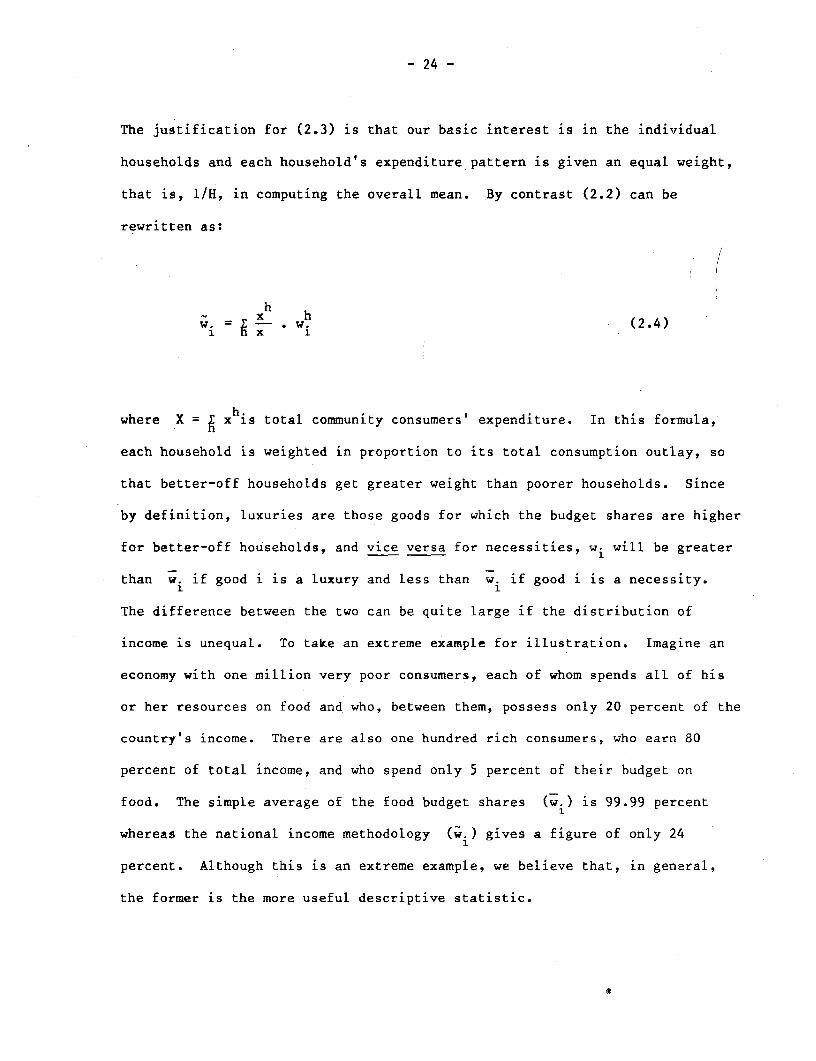
The justification for (2.3) is that our basic interest is in the individual
households and each household's expenditure pattern is given an equal weight,
that is, 1/H, in computing the overall mean. By contrast (2.2) can be
rewritten as:
h
= h x * w (2.4)
where X = h xhis total community consumers' expenditure. In this formula,
each household is weighted in proportion to its total consumption outlay, so
that better-off households get greater weight than poorer households. Since
by definition, luxuries are those goods for which the budget shares are higher
for better-off households, and vice versa for necessities, wi will be greater
than wi if good i is a luxury and less than wi if good i is a necessity.
The difference between the two can be quite large if the distribution of
income is unequal. To take an extreme example for illustration. Imagine an
economy with one million very poor consumers, each of whom spends all of his
or her resources on food and who, between them, possess only 20 percent of the
country's income. There are also one hundred rich consumers, who earn 80
percent of total income, and who spend only 5 percent of their budget on
food. The simple average of the food budget shares (w.) is 99.99 percent
whereas the national income methodology (wci) gives a figure of only 24
percent. Although this is an extreme example, we believe that, in general,
the former is the more useful descriptive statistic.
- 25 -
Illustrative Numbers from Three Surveys
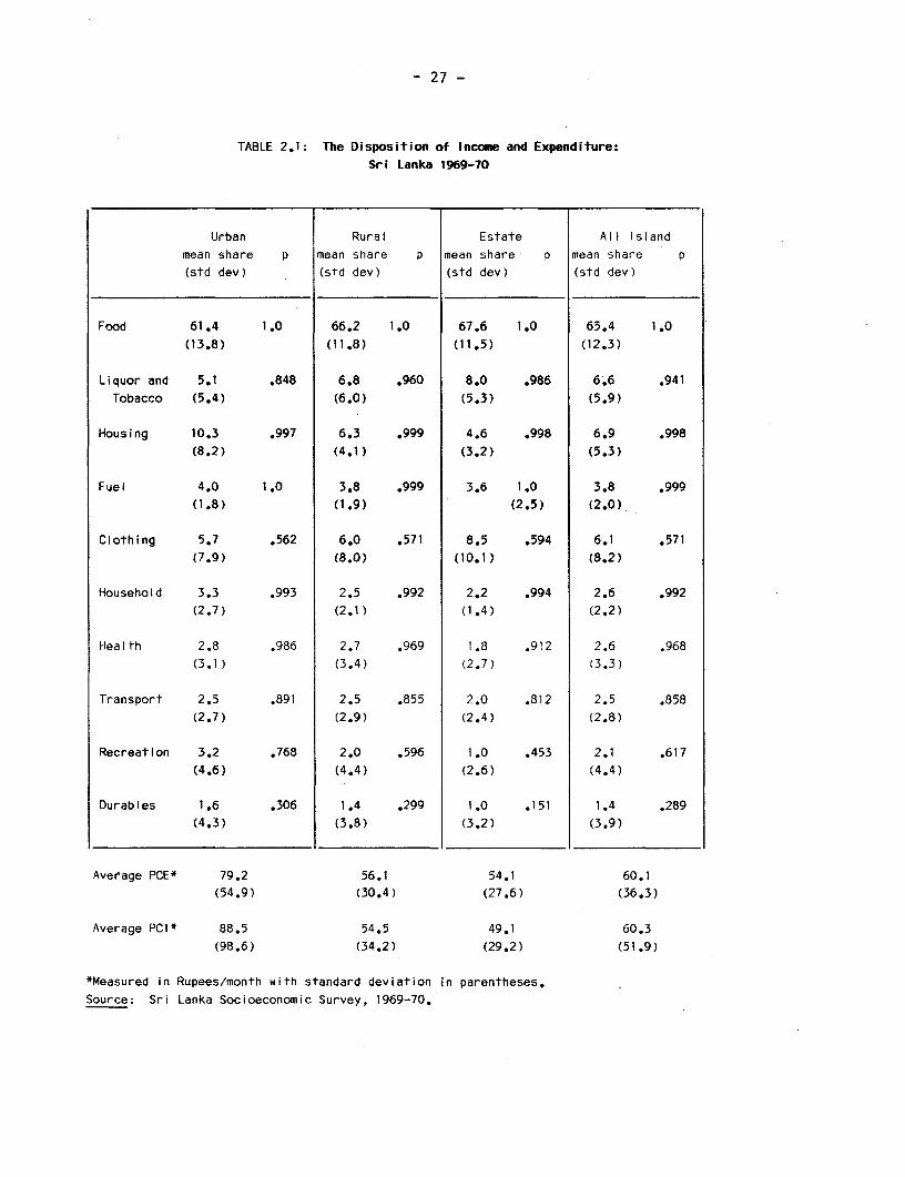
Tables 2.1, 2.2, and 2.3 are illustrative of the descriptive
tabulation of the disposition of income and expenditures that can be done
immediately after the survey results have been cleaned and collated. These
are based on three illustrative surveys, the 1969-70 and the 1980-81
Socioeconomic Surveys of Sri Lanka and the 1978 SUSENAS survey of Indonesia.
All three surveys, as is usual, are stratified. In the Sri Lankan cases,
there are three strata. The urban/rural dichotomy is standard enough, but the
third, estate, sector calls for brief comment.
These estates, largely tea estates, are economically, racially and
physically distinct from the rest of the island. The workers are of Indian
Tamil stock, they are typically very poor with relatively little inequality,
they have rather small families, atypically poor housing conditions, few
opportunities for own-account cultivation, and are employed, both men and
women, exclusively on the estates. In Sri Lanka, they form a natural third
sector for analysis which we expect to look rather different from the other
two.
The 1969-70 Sri Lanka survey covered 9,663 responding households,
4,022 from urban areas (population 375,000 households), 3,652 from rural areas
(population 1,696,000) and 1,990 from the estates (population 302,000); note
the unequal sampling weights, again a common feature given the cost
differences in collecting the data. The 1980-81 survey has 5,035 responding
households, 1,014 urban (population 570,000), 3,639 rural (population
2,264,000) and 382 estate (population 224,000). The Indonesian survey is
stratified more conventionally, both by urban and rural, and by geographic
region, into Java on the one hand and the Outer Islands on the other. There

- 26 -
are 6,351 households in total, 1,057 in urban Java (which contains 11 percent
of the country's households), 1,336 in rural Java (55 percent), 1,771 in urban
non-Java (6 percent), and 2,187 in rural non-Java (28 percent).
Use of these three surveys, here and in the following chapters,
allows us not only to examine the economic evolution of one country and the
change in the welfare of specific groups within its borders, but also to
compare the relative living standards and economic behavioral patterns of
households in two different countries.
The first tables give budget shares for various commodity groupings,
both by sectors, and for the whole economy. Proportions of households who
made non-zero purchases are also shown, as are the standard deviations of the
budget shares (including the zeros). Note that zero consumption of a good may
be an indication that the household never buys the good (for example, alcohol
in Indonesia), or that it simply happened not to do so over the period of the
survey (for example, clothing). Some goods, for example transport, may be
infrequently purchased by some households and never purchased by others.
The tables also give the averages of per capita expenditure, and per
capita income. The income and implied savings figures should be treated with
great caution because of likely understatement of income and possible
overstatement of consumption.
- 27 -
TABLE 2.1: The Disposition of Income and Expenditure:Sri Lanka 1969-70
Urban Rural Estate All Island
mean share p mean share p mean share p mean share p
(std dev) (std dev) (std dev) (std dev)
Food 61.4 1.0 66.2 1.0 67.6 1.0 65.4 1.0
(13.8) (11.8) (11.5) (12.3)
Liquor and 5.1 .848 6.8 .960 8.0 .986 6.6 .941
Tobacco (5.4) (6.0) (5.3) (5.9)
Housing 10.3 .997 6.3 .999 4.6 .998 6.9 .998
(8.2) (4.1) (3.2) (5.3)
Fuel 4.0 1.0 3.8 .999 3.6 1.0 3.8 .999(1.8) (1.9) (2.5) (2.0)
Clothing 5.7 .562 6.0 .571 8.5 .594 6.1 .571(7.9) (8.0) (10.1) (8.2)
Household 3.3 .993 2.5 .992 2.2 .994 2.6 .992(2.7) (2.1) (1.4) (2.2)
Health 2.8 .986 2.7 .969 1.8 .912 2.6 .968(3.1) (3.4) (2.7) (3.3)
Transport 2.5 .891 2.5 .855 2.0 .812 2.5 .858(2.7) (2.9) (2.4) (2.8)
Recreation 3.2 .768 2.0 .596 1.0 .453 2.1 .617(4.6) (4.4) (2.6) (4.4)
Durables 1.6 .306 1.4 .299 1.0 .151 1.4 .289
(4.3) (3.8) (3.2) (3.9)
Average PCE* 79.2 56.1 54.1 60.1(54.9) (30.4) (27.6) (36.3)
Average PCI* 88.5 54.5 49.1 60.3
(98.6) (34.2) (29.2) (51.9)
*Measured in Rupees/month with standard deviation in parentheses.
Source: Sri Lanka Socioeconomic Survey, 1969-70.
- 28 -
TABLE 2.2: The Disposition of Income and Expenditure:
Sri Lanka 1980-81
Urban Rural Estate All Island
mean share p mean share p mean share p mean share p
(std dev) (std dev) (std dev) (std dev)
Food 66.67 1.0 70.79 1.0 73.34 1.0 70.17 1.0
(13.23) (10.61) (8.07) (11.16)
Liquor and 3.92 .686 4.66 .865 5.86 .896 4.59 .833
Tobacco (5.12) (4.74) (4.25) (4.81)
Housing 7.35 1.0 4.07 1.0 3.08 1.0 4.63 1.0
(7.47) (3.83) (2.06) (4.85)
Fuel 5.72 .998 6.42 1.0 6.55 1.0 6.30 .999
(3.04) (2.96) (2.51) (2.96)
Clothing 3.74 .802 3.97 .854 4.50 .870 3.96 .845
(4.08) (3.55) (3.54) (3.66)
Health 2.65 .950 2.72 .932 1.95 .921 2.66 .935
(2.63) (3.48) (2.18) (3.27)
Transport 4.37 .739 3.04 .759 1.65 .663 3.21 .750
(7.26) (4.90) (2.51) (5.36)
Recreation 2.18 .642 1.39 .557 0.86 .429 1.51 .565
(3.85) (2.82) (2.15) (3.03)
Communication 0.22 .354 0.08 .263 0.06 .197 0.11 .276
(0.62) (0.23) (0.15) (0.34)
Household 3.19 .985 2.85 .987 2.16 .983 2.88 .986
Goods (4.41) (3.93) (1.44) (3.93)
Average PCE* 322.51 241.72 218.61 255.50
(247.8) (169.5) (113.3) (186.9)
Average PCI* 278.84 186.91 189.43 204.34
(336.1) (175.3) (110.6) (215.3)
*Measured in Rupees/month with standard deviation in parentheses.
Source: Sri Lanka Socioeconomic Survey, 1980-81.

- 29 -
TABLE 2.3: The Disposition of Income and Expenditure:
Indonesia 1978
Urban Rural Urban Rural All
Java Java Outer Islands Outer Islands Indonesia
mean share p mean share p mean share p mean share p mean share p |
(std dev) (std dev) (std dev) (std dev) (std dev)
Food 57.89 1.0 71.24 1.0 67.81 1.0 75.37 1.0 70.75 1.0(24.78) (36.12) (8.80) (13.63) (10.94)
Liquor 0.02 .01 0.05 .01 0.10 .03 0.23 .05 0.10 .02(0.56) (2.80) (0.62) (1.60) (0.83)
Tobacco 5.32 .68 5.06 .82 6.10 .73 5.62 .82 5.31 .80(10.19) (15.82) (4.33) (5.96) (4.44)
Housing 14.34 1.0 3.59 1.0 10.26 1.0 5.62 1.0 5.71 1.0(20.68) (15.87) (5.75) (6.53) (6.22)
Fuel 5.61 1.0 9.34 1.0 4.40 1.0 3.59 1.0 7.04 1.0(5.90) (16.69) (2.08) (3.60) (4.47)
Household 7.72 .97 3.55 .87 5.16 .95 2.73 .86 3.87 .88Goods (11.77) (18.24) (4.16) (4.82) (4.91)
Transport 3.16 .46 0,63 . 0.91 .22 0.25 .08 0.81 .15(9.50) | 8.50) (2.15) i1.56) (2.61)
Clothing 4.34 .98 5.26 .95 4.34 .94 5.28 .93 5.11 .95
(8.96) (20.15) (3.49) (8.12) (5.39)
User Taxes 1.60 .83 1.27 .61 0.94 .51 1.31 .44 1.30 .58
(3.98) (9.80) (1.44) (3.95) (2.59)
Average PCE* 10011 3881 8069 6095 5406(10892.1) (2505.9) (5793.7) (3973.9) (5173.3)
Source: SUSENAS 1978.

- 30 -
Even these rather basic data tell us a great deal about the
characteristics of the society and about the patterns of luxuries, necessities
and the incidence of poverty. Looking first at Sri Lanka in 1969-70, note the
dominant part in the budget of the food share, from 61 percent in the cities
to 68 percent in the estates. Note too that this ordering is the inverse of
the ranking according to per capita expenditure (PCE); both criteria rank the
estates as the poorest sector with the urban sector as the best-off. There is
substantially more inequality in the cities, whether judged by the standard
deviation of the food share in relation to its mean or by the same statistic
for PCE. The 30-40 percent of expenditure not devoted to food is spread
relatively equally over the other nine categories. In the urban sector,
housing is the second most important item of expenditures; housing, clothing
and liquor are about equally important in the rural sector; in the estates,
liquor and clothing come second, reflecting the relative cheapness (and low
quality) of estate-provided housing. Such patterns and rankings are
characteristic of very low income economies.
Turning to the proportions of households that make positive
purchases, virtually all households purchase food, housing, fuel, household
goods, health and, except in the cities, liquor. The vast majority of
households spend something on transport, even on the estates; clearly such
expenditure is not avoidable, even by the very poorest households. The
proportion of households making recreational expenditures varies dramatically
across the sectors, as does its share in the total; the same is true of
durables although, even in the cities, only 31 percent bought such goods at
all in the previous year. This first look at the data suggests that both
goods are luxuries, although the availability of various types of recreational

- 31 -
goods is also likely to have been important. Clothing is purchased by about
60 percent of households; such a figure reflects the length of the survey
recall period, not the fact that 40 percent of households do not buy
clothes. Finally, it is worth noting the variation in shares over households
within sectors. Food and fuel have the lowest coefficients of variation, as
would be expected of necessities. The high variation goods are also the
luxuries (that is, durables and recreational expenditures) and clothing (where
timing of purchases is important), with health and liquor expenditures in an
intermediate position. Notice that goods with high variation are also those
purchased by relatively few households; the censoring of the distribution at
zero tends to cause bimodality and high variation.
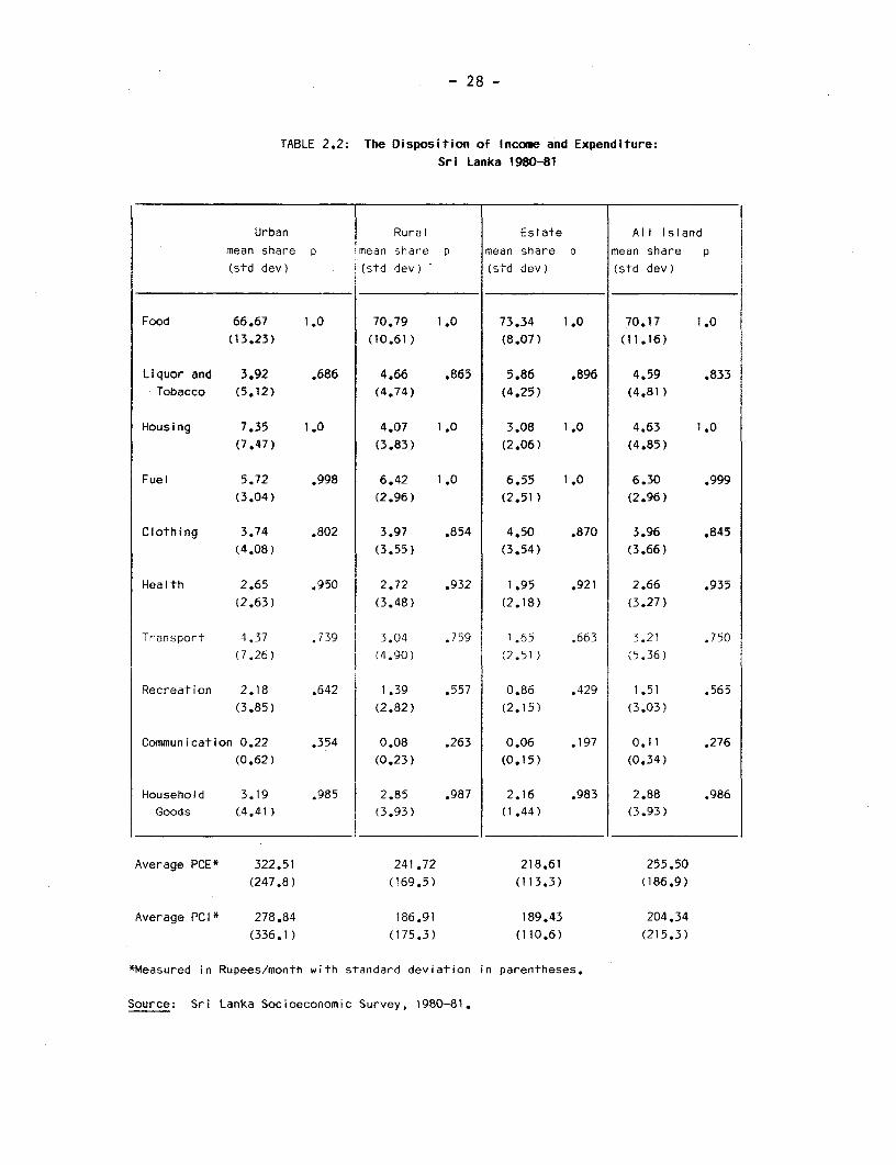
Table 2.2 presents the budget shares of various commodities for the
Sri Lanka 1980-81 survey. Although only the disposition of non-durable
expenditures is presented in Table 2.2, the patterns revealed are similar to
those of the earlier survey: food accounts for approximately 70 percent of
average household expenditure, with three categories, liquor and tobacco,
housing, and clothing, accounting for the majority of the remainder. The
estates continue to be distinguished as the poorest sector, whether measured
by the share of total expenditure devoted to food (73 percent in the estates,
compared to 71 percent for the rural and 67 percent for the urban sectors) or
by the average PCE, where the estates lag the rural and urban sectors by 11
percent and 48 percent respectively. As was true in the earlier survey, the
lowest coefficients of variation are displayed by food and fuel, necessities
purchased by all households during the sample period, and the highest by
communication, recreation and transport.
- 32 -
A comparison of Tables 2.1 and 2.2 suggests that within the decade
bounded by the surveys, households in all three sectors may have experienced
declines in their living standards. Food shares increased on average from 65
percent in 1969-70 to 70 percent in 1980-81, with approximately a 5 percentage
point increase in each sector. The change in food share yields a rule of
thumb estimate of the change in real PCE. Empirically, the change in the food
share has been found to equal approximately -15 percent of the change in
lnPCE, (see Chapter III for further discussion). Hence, disregarding changes
in relative prices, or the possible effects of changes in rationing schemes, a
5 percent increase in food share suggests an approximate decline in real PCE
of 30 percent. The shares of fuel and transport also increased, with fuel
rising from 3.7 percent to 6.3 percent of total non-durable expenditure, and
transport from 2.4 percent to 3.2 percent. These increases correspond to a
decline in the expenditure shares of all other goods; the shares of housing,
clothing, recreation, liquor and tobacco each fell roughly by 30 percent of
their 1969-70 figures.
There are many possible reasons for these shifts. If nominal incomes
did not keep pace with price increases, the resulting real income losses would
make themselves felt in living standards measures. Thus increases in fuel and
transport shares may be a reflection of the oil price increases in the
1970s. Further, changes in the Sri Lankan food rationing system during the
decade may, in part, be responsible for the marked increase in food shares.
In addition, the seasons in which the second survey was administered may have
biased the fuel and food shares: while the 1969-70 survey averaged one whole
year, the 1980-81 data comes only from October-December 1980 and January-April

- 33 -
1981; there m therefore be seasonal effects. A check of the 1969-70 survey,
however, showed little variation in expenditure shares by time of year.
In spite of somewhat different definitions, Table 2.3 can be employed
to note many of the similarities and differences between Sri Lanka and
Indonesia. In Indonesia, once again food accounts for the dominant share of
expenditure, and the country average of 70.8 percent is almost identical to
that of the later Sri Lankan survey. The share is again lower in urban areas,
and higher in the poor regions. However, in Indonesia, there appears to be
greater disparity between sectors. The urban Javanese food share is a full 20
percent below the national average. In contrast, note than in Sri Lanka 1980-
81, the greatest differences between any one sector's food share and the
national average was the 5 percent difference for the urban sector. One of
the major differences between the two countries is in the travel category.
Overall in Indonesia, only 14.5 percent of households registered travel
related expenditures; the corresponding Sri Lankan figure for 1969-70 was 85.8
percent. In urban Java, the average travel share was 3.2 percent. However,
given that half of the urban Javanese recorded zero purchases, we know that
many households spent a significantly greater proportion of their budgets on
travel than the urban average suggests. This is confirmed both by Figure 2.1,
which shows the relationship between the share of expenditure devoted to
travel and PCE, and where it can be seen that a noteworthy number of
households allocated between 5 percent and 15 percent of their expenditures on
travel.
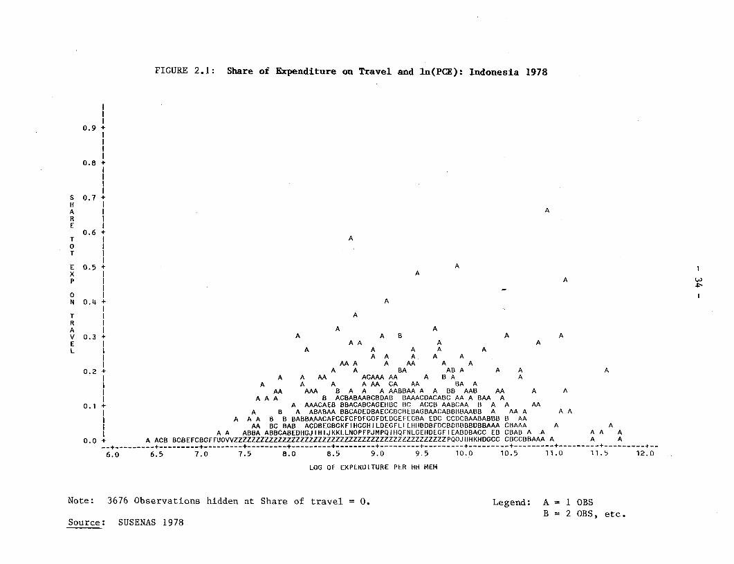
FIGURE 2.1: Share of Expenditure on Travel and ln(PCE): Indonesia 1978
0.°9+
0.8 +
S 0.7 +H |A AR |E I
0.6 +T IA0T |
E 0.5 + Ax AP IA J
0 IN 0.4 + A
T I AR IA | A AV 0.3+ A A B A AE A A A A AL | A A A A A
A A A A A A| M~~~~~~~~~~~~~A A A AA A A
0.2 + A A BA AB A A A AA A AA ACAAA AA A B A A
i A A A AA CA AA BA AAA MA B A A AAABBAA A A BB AAB AA A A
A A A B ACBABAABCBDAB BAAACDACABC AA A BAA A0.1 + A AMCAEB BBACABCAGEHBC BC ACCB AABCAA B A A AA
A B A ABABAA BBCADEDBAECCBCBEBAGBAACABBBBAABB A AA A A AA A A B B BABBAAACAFCCFCFDFCGFDEDGEFECBA EDC CCDCBAABABBB B AA
AA BC BAB ACDBEGBGKFIHGGHILDEGFLFEHIIBDBFDCBDBBBBDBBAAA CBAAA A AA A ABBA ABBCABEDHGJIHIJKKLLNOPFPJMPQIHQFNLGEHDEGFIEABDBACC EB CBAB A A A A A
0.0 + A ACB BCBEFCBGFFUOVVZZZZZZZZZZZZZZZZZZZZZZZZZZZZZZZZZZZZZZZZZZZZZZZZPQOJHHKHDGCC CBCCBBAAA A A A-_+--______+_____-___+____---+-__ -__ _+______-__+___ - +_ ------ _--+------+--_---++---____+_________+__
6.0 6.5 7.0 7.5 8.0 8.5 9.0 9.5 10.0 10.5 11.0 11.5 12.0
LOG OF EXPENDITURE PER HH MEM
Note: 3676 Observations hidden at Share of travel = 0. Legend: A = 1 OBS
B = 2 OBS, etc.Source: SUSENAS 1978
- 35 -
Returning to Table 2.3, note that almost no Indonesian households
purchase alcohol (or at least confess to doing so); Java is almost entirely
Muslim, the rest of the country largely so. Housing takes up a higher share
of the budget in urban areas, as is the case in Sri Lanka while other
expenditure items, namely tobacco, fuel, household goods (which here include
health expenditures) and clothing, also conform to the patterns discussed
above.
The food shares shown here for Sri Lanka and Indonesia are typical
for poor countries so that much of the interest in household budgets attaches
to the allocation of food expenditure itself. Table 2.4, for the Indonesian
survey, is reproduced from Chernichovsky and Meesook (1982) and shows the
breakdown of the food share into its components with disaggregation by
regions, by urban and rural, by seasons, and by expenditure class.
Chernichovsky and Meesook describe these figures as follows:
The urban population spends proportionately less on rice,corn, and cassava (the main staples) than does the ruralpopulation, and more on meat and poultry, eggs, milk,legumes, fruits and "other" foods. Similarly, the lower40 percent allocates more of its budget to the stap'lefoods than do the other expenditure groups, while theupper 30 percent spends relatively more on fish, meat andpoultry, eggs, milk, and "other" fQods. Within staples,the rural population spends a smaller proportion on riceand larger proportions on corn and cassava. The share ofstaples in the food budget declines while the share ofrice within the staple group increases with risingincomes.
They then go on to discuss the variations in shares by region (major) and by
season (minor).
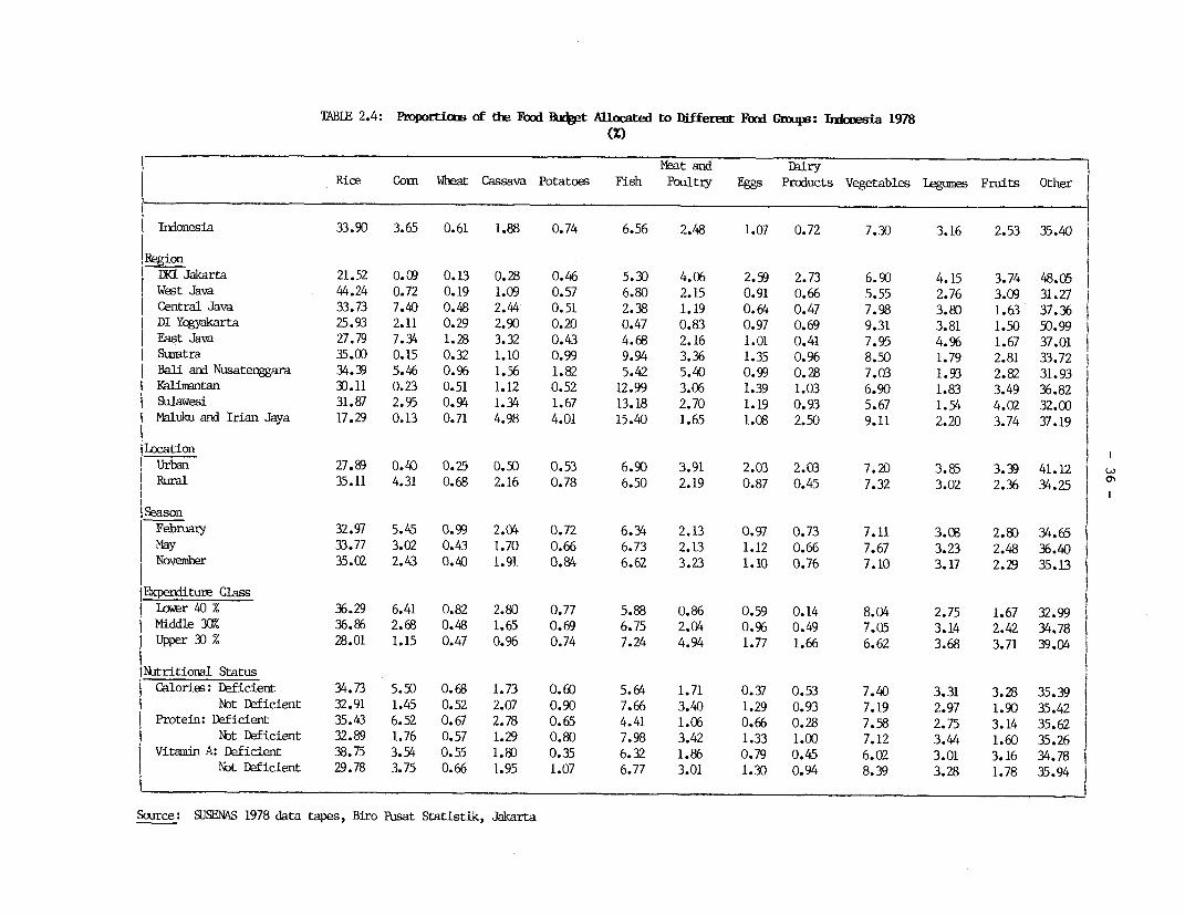
TABLE 2.4: Pwoportioos of the Food BHbdet Allocated to Different Food Groups: Indkxsia 1978
(Z)
Meat and DbiryRice Corm Wheat Cassava Potatoes Fish Poultry Eggs Products Vegetables Legmes Fruits Other
Indonesia 33.90 3.65 0.61 1.88 0.74 6.56 2.48 1.07 0.72 7.30 3.16 2.53 35.40
RegionDKE Jakarta 21.52 0.09 0.13 0.28 0.46 5.30 4.06 2.59 2.73 6.90 4.15 3.74 48.05West Java 44.24 0.72 0.19 1.09 0.57 6.80 2.15 0.91 0.66 5.55 2.76 3.09 31.27Central Java 33.73 7.40 0.48 2.44 0.51 2.38 1.19 0.64 0.47 7.98 3.80 1.63 37.36DI Yogyakarta 25.93 2.11 0.29 2.90 0.20 0.47 0.83 0.97 0.69 9.31 3.81 1.50 50.99East Java 27.79 7.34 1.28 3.32 0.43 4.68 2.16 1.01 0.41 7.95 4.96 1.67 37.01Sumatra 35.00 0.15 0.32 1.10 0.99 9.94 3.36 1.35 0.96 8.50 1.79 2.81 33.72Bali and Nusatenggara 34.39 5.46 0.% 1.56 1.82 5.42 5.40 0.99 0.28 7.03 1.93 2.82 31.93Kalimantan 30.11 0.23 0.51 1.12 0.52 12.99 3.06 1.39 1.03 6.90 1.83 3.49 36.82Sulawesi 31.87 2.95 0.94 1.34 1.67 13.18 2.70 1.19 0.93 5.67 1.54 4.02 32.00Maluku and Irian Jaya 17.29 0.13 0.71 4.98 4.01 15.40 1.65 1.08 2.50 9.11 2.20 3.74 37.19
LocationUrban 27.89 0.40 0.25 0.50 0.53 6.90 3.91 2.03 2.03 7.20 3.85 3.39 41.12 L
Rural 35.11 4.31 0.68 2.16 0.78 6.50 2.19 0.87 0.45 7.32 3.02 2.36 34.25
SeasonFebruary 32.97 5.45 0.99 2.04 0.72 6.34 2.13 0.97 0.73 7.11 3.08 2.80 34.65May 33.77 3.02 0.43 1.70 0.66 6.73 2.13 1.12 0.66 7.67 3.23 2.48 36.40November 35.02 2.43 0.40 1.91 0.84 6.62 3.23 1.10 0.76 7.10 3.17 2.29 35.13
Exenditure ClassLow,er 40 % 36.29 6.41 0.82 2.80 0.77 5.88 0.86 0.59 0.14 8.04 2.75 1.67 32.99Middle 3(if/ 36.86 2.68 0.48 1.65 0.69 6.75 2.04 0.96 0.49 7.05 3.14 2.42 34.78Upper 30 % 28.01 1.15 0.47 0.96 0.74 7.24 4.94 1.77 1.66 6.62 3.68 3.71 39.04
Nutritional StatusCalories: Deficient 34.73 5.50 0.68 1.73 0.60 5.64 1.71 0.37 0.53 7.40 3.31 3.28 35.39
Nbt Deficient 32.91 1.45 0.52 2.07 0.90 7.66 3.40 1.29 0.93 7.19 2.97 1.90 35.42Protein: Deficient 35.43 6.52 0.67 2.78 0.65 4.41 1.06 0.66 0.28 7.58 2.75 3.14 35.62
Nbt Deficient 32.89 1.76 0.57 1.29 0.80 7.98 3.42 1.33 1.00 7.12 3.44 1.60 35.26Vitamin A: Deficient 38.75 3.54 0.55 1.80 0.35 6.32 1.86 0.79 0.45 6.02 3.01 3.16 34.78
Nbt Deficient 29.78 3.75 0.66 1.95 1.07 6.77 3.01 1.30 0.94 8.39 3.28 1.78 35.94
Source: SJSENAS 1978 data tapes, Biro Pusat Statistik, Jakarta
- 37
Since one of the major covariates of the demand patterns is the size
of the household budget, the logical next step in description is to cross-
tabulate savings patterns, expenditure shares, and the allocation of the food
budget against total household expenditure. There are a number of possible
income or expenditure variables that could be used to measure each household's
command over resources, but here our preferred measure is household PCE.
There are good grounds for taking PCE as a short-run measure of economic
welfare (at least as an approximation); it fluctuates over time much less than
does income, and it tends to be more easily and more accurately measured than
is income. There is also a number of different ways of illustrating the
empirical joint distributions between the various magnitudes and PCE. Scatter
diagrams of individual observations can be useful, but are clumsy tools with
so many observations where patterns are more easily discerned if averages are
taken over different income groups. One of the most convenient ways of doing
this is to divide households by PCE deciles. By definition, households are
equally spread among the ten deciles, and the cross-tabulations tend to convey
most of the covariation with income, without either being tied to a specific
functional form or swamping the reader in an enormous amount of information.
Table 2.5 shows the ratios of expenditure to income in three surveys
discussed by Visaria, for Peninsular Malaysia 1973, for Sri Lanka 1969-70 (the
same survey used above) and for Taiwan 1974, and the Sri Lanka 1980-81 survey
used above. The A columns show average expenditure to income ratios for the
ten deciles of household per capita expenditure while the B columns give the
same information where the deciles are defined in terms of per capita
income. Although the saving or expenditure ratios differ among countries -
the savings ratios in Malaysia and Taiwan are about 15 percent, but the figure

- 38 -
TABLE 2.5: Expenditure to Income Ratios: Four Surveys
PeninsularMalaysia Sri Lanka Sri Lanka Taiwan
1973 1969-70 1980-81 1974Decile A B A B A B A B
1 0.704 3.683 0.990 1.340 1.347 2.918 0.883 0.996
2 0.869 1.241 1.000 1.247 1.505 1.951 0.879 0.944
3 0.885 1.115 0.995 1.188 1.515 1.720 0.886 0.923
4 0.893 1.070 1.008 1.145 1.596 1.588 0.874 0.921
5 0.925 0.987 1.051 1.100 1.656 1.499 0.864 0.903
6 0.858 0.987 0.996 1.070 1.587 1.421 0.864 0.881
7 0.918 0.882 1.055 1.012 1.626 1.314 0.861 0.858
8 0.871 0.844 1.047 0.976 1.667 1.236 0.852 0.840
9 0.715 0.808 1.038 0.936 1.644 1.136 0.804 0.808
10 0.859 0.581 0.926 0.772 1.620 0.928 0.806 0.706
All 0.845 0.845 1.003 1.003 1.576 1.576 0.849 0.849
Source: Visaria, LSMS Working Paper No. 2;Sri Lanka Socioeonomic Surveys, 1969-70 and 1980-81.

- 39 -
for Sri Lanka 1969-70 is -0.3 percent and for Sri Lanka 1980-81 is -57.6
percent (almost certainly because of understatement of income and possible
seasonal effects, though the more severe (reported) dissavings in the later
survey are consistent with the apparent lower real income in the later period
though they cannot be fully explained by it) - the picture over deciles is
remarkably uniform between the countries. Using income deciles, the saving
ratio declines steadily with income, most markedly in Malaysia and least so in
Taiwan. However, with expenditure deciles, saving ratios show little
variation over the groups. This finding is of course consistent with the view
that PCE measures welfare on a longer time scale than does per capita income
(PCI). Many households who find themselves in the low PCI deciles are there
temporarily, because of illness, unemployment, or a poor harvest. However,
because their position is temporary they have assets to fall back on,
collateral for loans, or relatively fortunate relatives or friends. They can
thus afford to spend more than their earnings to tide them over until good
times come again, or until the bad times are permanently established along
with a new, lower consumption level. By contrast, households that are poor by
the PCE criterion are more likely to be permanently poor and to have therefore
adjusted their consumption to their income. For them, as for everyone, some
saving is no less or more essential than purchases of other goods. Hence,
when ranked by PCE, households save much the same proportion of their income
regardless of their ranking.
Finally, we look briefly at patterns of demand by deciles. Table 2.6
gives the "All Island" pattern of expenditure by deciles in the Sri Lankan
1969-70 and 1980-81 surveys. A more systematic formal analysis of these
patterns will be presented in the next chapter which deals with the derivation
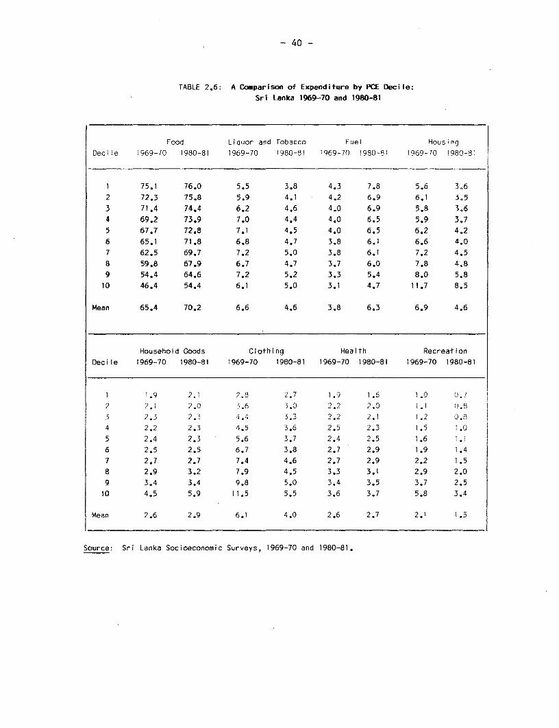
- 40 -
TABLE 2.6: A Comparison of Expenditure by PCE Decile:
Sri Lanka 1969-70 and 1980-81
Food Liquor and Tobacco Fuel Housing
Deci!e '969-70 1980-81 1969-70 1980-81 1969-70 1980-81 1969-70 980-81
1 75.1 76.0 5.5 3.8 4.3 7.8 5.6 3.6
2 72.3 75.8 5.9 4.1 4.2 6.9 6.1 3,5
3 71.4 74.4 6.2 4.6 4.0 6.9 5.8 3.6
4 69.2 73.9 7.0 4.4 4.0 6.5 5.9 3,7
5 67.7 72.8 7.1 4.5 4.0 6.5 6.2 4,2
6 65.1 71.8 6.8 4.7 3.8 6.1 6.6 4.0
7 62.5 69.7 7.2 5.0 3.8 6.1 7.2 4.5
8 59.8 67.9 6.7 4.7 3.7 6.0 7.8 4.8
9 54.4 64.6 7.2 5.2 3.3 5.4 8.0 5,810 46.4 54.4 6.1 5.0 3.1 4.7 11.7 8.5
Mean 65.4 70.2 6.6 4.6 3.8 6.3 6.9 4.6
Household Goods Clothing Health Recreation
Decile 1969-70 1980-81 1969-70 1980-81 1969-70 1980-81 1969-70 1980-81
1 !,9 2.1 2.8 2.7 1.9 1.6 1.0 0.7
2 2.1 2.0 3.6 3.0 2. 2 2.0 *1 0.8
3 2.3 2.3 4.4 3.3 2.2 2.1 1.2 0.8
4 2.2 2.3 4.5 3.6 2.5 2.3 1.5 1.05 2.4 2.3 5.6 3.7 2.4 2.5 1.6 1.16 2.5 2.5 6.7 3.8 2.7 2.9 1.9 1.4
7 2.7 2.7 7.4 4.6 2.7 2.9 2.2 1.58 2.9 3.2 7.9 4.5 3.3 3.1 2.9 2.0
9 3.4 3.4 9.8 5.0 3.4 3.5 3.7 2.5
10 4.5 5.9 11.5 5.5 3.6 3.7 5.8 3.4
Mean 2.6 2.9 6.1 4.0 2.6 2.7 2.1 1.5
Source: Sri Lanka Socioeconomic Surveys, 1969-70 and 1980-81.

- 41 -
of Engel curves. However, the main patterns are clear from the table. In the
1969-70 survey, the shares of food and fuel decline fairly steadily, with food
share falling from 75 percent in the lowest decile to 45 percent in the
highest. Liquor and tobacco maintain a relatively constant share across
deciles, while the shares of all other non-food items (led by housing) rise
with increases in PCE. These patterns are repeated in the 1980-81 survey, as
is evident from the lower portion of the table, and are very similar, in turn,
to the patterns revealed by the 1978 SUSENAS survey of Indonesia, presented in
Figure 2.2. The information here is much the same as in Table 2.6 but the
graphical form allows it to be more rapidly and more easily assimilated.
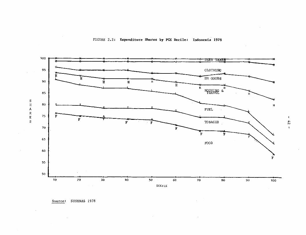
FIGURE 2.2: Expenditure Shares by PCE Decile: Indonesia 1978
100 . A K
95 CLOTHING
90
S~~~~~~~~~~~~~~~~~~~~~~HUS85
RAW &E£
A 80 L . I - - T,,,,,, . T T T v - - HARE 75
T F T *\
70
65
60
F55
50 t
10 20 30 40 50 60 70 80 90 100
DEC I LE
Source: SUSENAS 1978
- 43 -
Notes for Further Reading
More detailed analyses of these and other similar data can be found
in the papers by Visaria (1980), for a wide range of data sets, and by
Chernichovsky and Meesook (1982) for Indonesia. Recent papers by Bhalla
(1985), Glewwe and Bhalla (1985), and Anand (1985) attempt to sort out what
has actually happened to living standards in Sri Lanka since 1969; the task is
a very complex one and is beyond the scope of an illustrative chapter such as
this one. The suspicion that consumption may be overstated in household
surveys in LDC's comes from Bhattacharyya's (1963) study in which experiments
were carried out with questionnaires of varying amounts of detail. The more
commodities identified on the schedule, the more expenditure is reported. Of
course, this does not tell us whether the short schedules understate, or the
long ones overstate, or whether there is some combination.

- 44 -
CHAPTER III
THE ESTIMATION OF ENGEL CURVES
In this chapter, we present a methodology for the estimation of Engel
curves with particular emphasis on the relationship between food demand and
per capita household expenditure. The detailed results discussed here come
once again from the Sri Lankan 1969-70 and 1980-81 surveys and the 1978
SUSENAS survey of Indonesia.
As in the previous chapter, we take the explanation of the budget
shares as our primary task. The simplest possible model of demand that makes
any kind of sense is that which treats the budget shares as centered around
constants, that is
w = w. + u( t3.1)1 1~ 1
where i is a commodity subscript, h is a household subscript, and uhrepresents
the household deviation from the population mean w.. Almost all
"intelligent laymen" would use (3.1) as a starting point for projection. If
we want to know commodity demands in 1990, a sensible first guess is obtained
by applying the current expenditure pattern to the projected level of total
outlays in 1990. Even in a cross-section, (3.1) is not obviously false for a
number of commodities, excluding of course food.
However, even the most cursory inspection of the data, for example
those in Table 2.6, shows that expenditure patterns are not the same for rich

- 45 -
and poor households. Hence (3.1) must be extended to take account of the
influence of income, total expenditure and so on. Once again, we prefer a
measure of total expenditure rather than an income measure. We also deflate
by household size, in order to make at least a crude allowance for the greater
needs of larger households. At the next stage of analysis, we shall take a
more sophisticated approach to demographic composition. The immediate issue,
however, is to select a simple functional form that is consistent with the
data. There is no reason to suppose that the same functional form will work
well for all possible household surveys, but the procedure we adopt here
should be flexible enough to allow for this if carefully applied.
Food Shares and Total Expenditure
It is clear from Table 2.6 and Figure 2.2 that the major changes in
expenditure patterns with per capita expenditure are in the split between food
and non-food. A natural starting point, therefore, is to find a functional
form that can account for this split consistently with the data. Figure 3.1
shows the empirical joint distribution of the food share and per capita
household expenditure in the Sri Lankan 1969-70 survey. The solid lines are
contours of the distribution, hence, the highest point (the joint mode) is
around (65 percent, 50 rupees) and the mass tails off to the bottom right. We
would expect this sort of picture to be fairly typical; PCE normally has a
marginal distribution that is positively skewed while the food share is
somewhat negatively skewed although the skewness is much less than for PCE.
Given these features, the regression of the food share on PCE will be
nonlinear as shown. However, if PCE is approximately log-normally
distributed, much of the skewness can be removed by working with the logarithm

- 46 -
of PCE rather than with PCE itself. Figure 3.2 shows the same scatter as
Figure 3.1, but now with PCE measured on a logarithmic scale on the horizontal
axis. The contours now suggest that a linear regression is appropriate for
use with the Sri Lankan data. Scatter plots presented in Figure 3.2 reveal
that this also holds true for the Indonesian data although of course, in both
cases, much is left unexplained.
We therefore amend (3.1) to read:
h h hwi = a+ aln PCE + u i (3.2)
Although this form of Engel curve is often not included in comparative
studies, largely because Prais and Houthakker (1955) did not use it,
nevertheless it has been recommended, notably by Working (1943) and by Leser
(1963). It also has sound theoretical foundations, unlike many of the more
popular forms; these are discussed for example in Deaton and Muellbauer
(1980). -For our current purposes, an important feature of the formulation is
that, unlike most other empirical Engel curves, it meets the most obvious
requirement of an allocation model that, if applied to all goods in the
budget, its predicted budget shares add up to unity. From (3.2), this will
happen if:
= 1 f8. = 0 (3.3)11
Note too that for those commodities with ai> 0, the budget share increases
with PCE, for those with ai< 0, the share decreases, while if 8i = 0, the
share is independent of PCE. Hence, luxuries and necessities are naturally
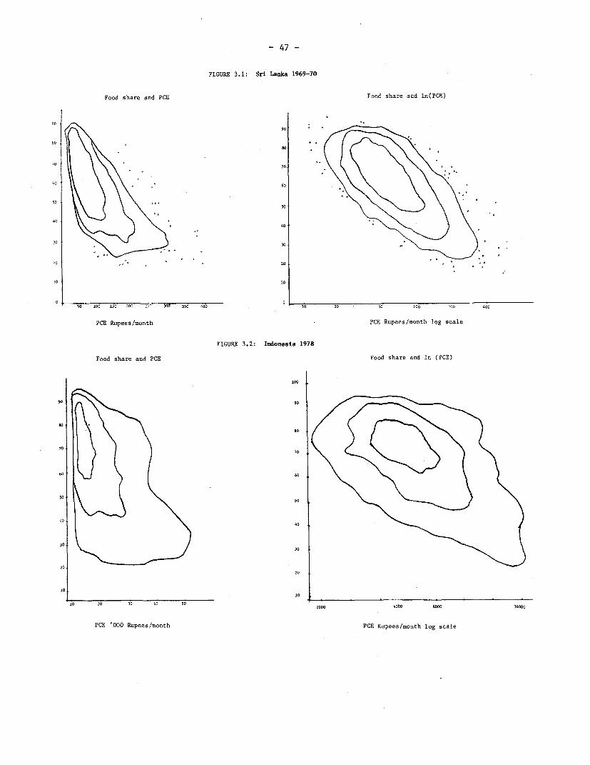
- 47 -
FIGURE 3.1: Sri Lanka 1969-70
Food share and PCE Food share and ln(PCE)
90
10010 80~~~~~~~~~~~~~~~~~~~~~~~~~~~~a
7070
6060
50
so
00
40
30 3
20 20
10 10
1 O 100 150 200 2 49 300 350 I000 20 50 000 200 400
PCE Rupees/month PCE Rupees/month log scale
FIGURE 3.2: Indonesia 1978
Food share and FCE Food share and In (FCE)
100
90 90
SDso
7070
00 60
s050
0040
30
30
20
00
10~~~~~~~~~~~~~~~~~~~~~~~~~~~~1
10 20 30 40 502000 4090 8000 36000
POE '000 Rupees/month PCE Rupees/month log scale
- 48 -
identified by the model, but perhaps more importantly we see clearly the role
of PCE as causing a reallocation of the budget as economic status improves.
Note finally that the adding-up conditions (3.3) should ideally hold for the
estimated parameters. It turns out to be unnecessary to make any special
allowance for this since ordinary least squares estimation (and a wide variety
of other procedures) will automatically generate estimates that satisfy (3.3).
Although the a parameters are dimensionless, and so can be compared
across time or across countries, it is often convenient (and is conventionally
done) to convert the si parameters to total expenditure elasticities. This
can be accomplished using the formula:
e. = 1 + B./w. (3.4)1 1 1
where ei is the total expenditure elasticity. Note that these elasticities
are not constant as wi and PCE vary, so that they are usually presented at the
sample mean of wi, where predicted and actual budget shares automatically
coincide. The formula (3.4) also implies that, if ei is not unity, then it
falls as PCE increases. This is simply an automatic feature of Engel curves
like (3.2) and it may or may not be true in reality. It can be tested by
extending the model in a way that we shall describe below.
Engel Curves for the Three Surveys
Tables 3.1, 3.2 and 3.3 present the estimated 8-coefficients, (with
standard errors) together with expenditure elasticities evaluated at the
sample mean for the Sri Lankan and Indonesian surveys respectively.
Estimation can be carried out either using all the observations or discarding

- 49 -
TABLE 3.1: B-Coefficients, Standard Errors, and Expenditure Elasticities:Sri Lanka 1969-70
Urban Rural Estate All IslandB e B e B e B e
(s. e.) (s.e.) (s.e.) (s. e.)
Food -18.58 0.70 -16.00 0.76 -14.08 0.79 -16.08 0.75(0.26) (0.34) (0.55) (0.32)
Liquor and 0.33 1.06 1.41 1.21 1.90 1.24 0.62 1.09Tobacco (0.15) (0.22) (0.29) (0.20)
Housing 6.60 1.64 1.19 1.19 -0.58 0.87 3.02 1.44(0.20) (0.15) (0.18) (0.17)
Fuel -0.70 0.82 -0.68 0.82 -1.51 0.58 -0.67 0.82(0.05) (0.07) (0.13) (0.07)
Clothing 4.38 1.77 5.92 1.99 8.90 2.05 5.08 1.83(0.21) (0.27) (0.51) (0.27)
Household 1.61 1.49 1.12 1.45 0.37 1.16 1.31 1.50(0.07) (0.07) (0.08) (0.07)
Health 0.78 1.28 1.06 1.39 1.08 1.60 1.02 1.39I (0.09) (0.12) (0.15) (0.11)
Transport 0.83 1.32 1.44 1.58 0.94 1.47 1.22 1.50(0.08) (0.10) (0.13) (0.09)
Recreation 2.56 1.80 2.38 2.19 1.35 2.35 2.46 2.16(0.12) (0.16) (0.14) (0.14)
Durables 2.21 2.38 2.15 2.54 1.73 2.73 2.03 2.46(0.12) (0.14) (0.17) (0.13)
Source: Sri Lanka Socioeconomic Survey, 1969-70.

- 50 -
TABLE 3.2: $-Coefficients, Standard Errors, and Expenditure Elasticities:Sri Lanka 1980-81
Urban Rural Estate All Island8 e 3 e 8 e 8 e
(s.e.) (s.e.) (s.e.) (s.e.)
Food -15.37 0.77 -10.74 0.79 -5.14 0.93 -11.72 0.84(0.49) (0.31) (0.97) (0.25)
Liquor and -0.05 0.99 0.89 1.19 -1.75 1.30 0.68 1.15Tobacco (0.27) (0.16) (0.52) (0.13)
Housing 5.29 1.72 1.35 1.33 -0.96 0.69 2.25 1.49(0.36) (0.13) (0.25) (0.12)
Fuel -2.04 0.64 -1.37 0.79 -1.14 0.83 -1.54 0.76(0.15) (0.10) (0.31) (0.08)
Clothing 1.75 1.47 1.63 1.41 2.05 1.45 1.68 1.42(0.21) (0.12) (0.43) (0.10)
Household 2.19 1.69 2.03 1.71 0.48 1.22 2.03 1.71(0.22) (0.13) (0.18) (0.10)
Health 1.05 1.39 1.35 1.49 0.48 1.25 1.24 1.47(0.13) (0.11) (0.26) (0.09)
Transport 4.73 2.08 3.53 2.16 1.64 2.00 3.78 2.18(0.35) (0.15) (0.30) (0.14)
Recreation 2.10 1.96 1.24 1.89 0.73 1.85 1.44 1.95(0.19) (0.09) (0.27) (0.08)
Communication 0.36 2.64 0.09 2.18 0.10 2.60 0.16 2.48(0.03) (0.01) (0.02) (0.01)
Source: Sri Lanka Socioeconomic Survey, 1980-81

- 51 -
TABLE 3.3: s-Coefficients, Standard Errors, and Expenditure Elasticities:
Indonesia 1978
Urban Rural Urban Rural All
Java Java Outer Islands Outer Islands Households
e e 6 e a e 6 e
(s.e.) (s.e.) (s.e.) (s.e.) (s.e.)
Food -12.35 0.79 -8.41 0.88 -9.99 0.85 -4.97 0.93 -8.39 0.88(0.47) (0.60) (0.46) (0.38) (0.24)
Liquor 0.03 2.25 0.18 4.58 0.07 1.74 0.22 1.94 0.15 2.54(0.01) (0.05) (0.04) (0.05) (0.02)
Tobacco -0.15 0.97 1.46 1.29 0.93 1.15 1.02 1.13 0.96 1.18(0.25) (0.28) (0.26) (0.17) (0.12)
Housing 6.86 1.48 2.25 1.63 3.35 1.33 0.37 1.07 2.92 1.51(0.45) (0.28) (0.33) (0.19) (0.14)
Fuel -2.06 0.63 -2.99 0.68 -0.40 0.91 -0.63 0.83 -2.16 0.69(0.13) (0.29) (0.12) (0.10) (0.10)
Household 2.69 1.35 2.51 1.71 2.78 1.54 1.08 1.40 2.19 1.57
(0.27) (0.32) (0.24) (0.14) (0.12)
Transport 2.75 1.87 1.08 2.71 1.31 2.44 0.15 1.60 1.22 2.51
(0.21) (0.15) (0.12) (0.05) (0.06)
Clothing 1.41 1.32 3.54 1.67 1.55 1.36 2.14 1.41 2.56 1.50
(0.21) (0.34) (0.20) (0.23) (0.14)
User Taxes 0.83 1.52 0.38 1.30 0.40 1.43 0.62 1.47 0.56 1.43(0.09) (0.17) (0.09) (0.11) (0.07)
Source: SUSENAS 1978.

- 52 -
those recording zero purchases. Both procedures can cause bias if there are
substantial numbers of zeros, and the results here are based on all the
observations. A rough (and somewhat unreliable) correction for bias can be
made by dividing the 8's by the corresponding proportions of recorded
purchases, given in Tables 2.1 to 2.3. Taking the Sri Lankan (1969-70) urban
sector as an example, estimated elasticities would become: for transport, 1.36
(rather than the figure shown of 1.32); for recreation, 2.04 (1.80); for
clothing, 2.37 (1.77); and for durables, 5.51 (2.38).
Table 3.1 suggests very strongly that, for Sri Lanka in 1969-70,
virtually none of the budget shares are constant as PCE changes.
All a's, except for liquor and tobacco in the urban sector, are different from
zero at a very high level of significance so that all the total expenditure
elasticities are different from one. Food and fuel are the two necessities,
whose shares in the budget drop with PCE. Additionally, housing is a
necessity in the estates, perhaps reflecting the essentially uniform provision
of low quality housing to estate workers. All other goods are luxuries and,
by and large, the poorer the sector the more luxurious are the luxury goods.
The large number of expenditure categories which are accounted as luxuries is
again typical of developing countries and is essentially a consequence of the
dominant role of food in the budget. For the very poor, everything but food
(and fuel) is a luxury.
Although classifications differ slightly between surveys, Table 3.2
reveals patterns for Sri Lanka 1980-81 that are quite similar to those of the
earlier survey. Again, the budget shares of all goods change with PCE - with
the possible exception of liquor in the urban sector - and, in both surveys,
the same goods are identified as necessities, namely food and fuel in all
- 53 -
sectors and housing on the estates. However, while the directions of the
anticipated budget reallocations do not appear to have changed between 1970
and 1980, clearly the magnitudes of such reallocations did. This is evident
in cross survey comparisons of both the 8-coefficients and the expenditure
elasticities. As equation (3.4) states indirectly and (3.5) directly,
the a-coefficients predict the extent to which the budget allocation of an
additional rupee will differ from the present allocation of total household
expenditure (THE):
ai = 8(piqi)/a(THE) - wi (3.5)
Thus the change in the 6-coefficient on food (which rose from -16.1
to -11.7 nationally) indicates that households in 1980-81 would be less able
to allocate away from food if allowed a marginal increase in expenditure. For
the island as a whole in 1970, a 100 rupee increase in total household
expenditure would have resulted in an increase in food expenditure of 49
rupees. In 1980, this figure rose to 59 rupees. A second substantial change
in the allocation of budgets at the margin occurred in transport; marginal
expenditure for this category doubled during the decade, rising from 3.7 to
7.0 rupees. That these "necessities", food and (loosely) transport, claim a
significantly larger portion of a marginal increase in household expenditure
is again consistent with an overall decline in household living standards
between the two surveys. Note that the increases in the marginal propensities
to spend on food and transport are offset by declines in luxury items, notably
housing, clothing, and recreation.
- 54 -
The results in Table 3.3 paint a picture of Indonesia in 1978 which
is broadly similar to that of Sri Lanka in 1980-81. As in Sri Lanka, food and
fuel are the two obvious necessities and, when discussing the country as a
whole, the expenditure elasticities of luxuries observed in Indonesia are
roughly the same as those in the later Sri Lankan survey: for housing (1.51 in
Indonesia, compared to 1.49 in Sri Lanka 1980-81); for clothing (1.50 to
1.42); for household goods (1.57 to 1.71); for transport (2.51 to 2.18); and
that of tobacco in Indonesia (1.18) might be comparable to that of alcohol and
tobacco in Sri Lanka (1.15). Alcohol in Indonesia comes out as highly
expenditure elastic - presumably religious conventions are only ignored by
relatively wealthy individuals.
The Indonesian regression results reveal striking differences in
household behavior between sectors. For example, the s-coefficient on food in
urban Java (-12.35) is more than twice that of the rural outer islands
(-4.97). The scatter plots of food share and ln(PCE) presented in Figure 3.3
indicate why this occurs. In Figure 3.3, note the enormous amount of
individual variation which is reflected in the low R2-statistics that are
typical in the anaLysis of large microeconomic samples such as these. While
such randomness is unavoidable, given the idiosyncrasies of household economic
behavior, it does not obscure basic patterns of that behavior. For example,
in Figure 3.3, it is clear that the food share in urban Java falls more
rapidly with increases in PCE and is more closely related to PCE than is the
case for food shares in the other sectors. The rural outer islands are at the
opposite extreme with a much wider scatter and a less close relationship.
These types of diagrams can prove to be extremely useful, both for suggesting

- 55 -
suitable functional form and for aiding the interpretation of both descriptive
statistics and regression results.

- 56-
FIGURE 3.3: Food Share: Indouesia 1978
Urban Java Rural Java
Food FoodShare Share
1.0
0.9 ~~~~~~~~~~~~~~~~~~~~~~~1.00.9~~~~~~~~~~~~~~~~~~~~~.
0.8 ~ ~ A AA AA A A0. A A A
0.81 * SAAA CAACA A A AAACA ABCAA SAC ASS AAA.80.7~ ~ ~ *A * 9 * AA9 AA0ASAAACA8MAAA
CA A*ASAA BAASAAA AAAAA AAAAAAA AASMA BAOAA AA CAB 0AS70.6 ~ ~ ~ ~ ~ ~ ~ ~ ~ ~ ~ ~ ~ ~ ~ ~ ~~~~~~~~~~~*. ACAAAMA0ACMAAAA A8 B BA
0.7 I A BAA.AAA AAASAABAABAAA a 9*5*8(0850CM CAMSAAAC MA *80 - A6
0.63A ACACA SACMACAAAAAAAA A SA S AB.A 8 AA CA AC A AAM8SCAAMAA 580 AA3
0.2 ~ ~ ~ AAA AAAAS8ACOS08*8AACA ACACBCSCAAAA
BAA AAA.ACACACS A 089 CAA8CAAMA A A0 AAAASCAAA0AAAAAS2MSC 0.1 ~ ~ ~ ~ AAAAABASAAABA AB AAAAA ACSA A M AC
BAAAAACABCAAAAC8BAB ACACA A A A AAAA S 888*0 850 A*AA------- ----- A----- ----BAA -----------A ---- CA ---------------------- AS A---A--A--A -A-A-A----------C MA---- ------------------- CA... S------------
1000 2000 40A CA AA1MABA 32A000 600AACA 10 A20 A A 000 C OCA 1AA0A
0.9 1.~~~~~~~~~~~~~~~~~~~~~~0.
0.6 ~~~~~~~~~~~~~~~ A 0.9
0170.1
10000 40 00160 20 600 700 20 0080 60
1.0~~~~~~~~~~~~~~~~~~~~~~.
0.2 . AA .
0 1..... ..... ..... ......A..B....A... . .A....BAA...A..-B- ----A.2.A... ..... C. A..... .. . ..... . --.. ...... ... .- ---- - --- --A-- -- -
1000 2000 4000 $000~~~ 16000A 32A000A M ASALA CA B A A00 00 CA0 A 60 20
A PerAA OAACACCAAAAAAA caitMepe BAur Ao Bcl e aiaepedtr o cl
So urce: ASU AANAS S1A978 AAB ABMOA A A M MAASASCAA AAMA A B

- 57 -
Engel Curves and Household Composition
These results, although helpful in systematizing the role of total
expenditure in modifying the household budget, are still very crude. The
estimates are likely to be biased, not just by the problems with zero
purchases, but also by the omission of a whole host of other factors. Some of
these are allowed for in the estimates since additive dummies for seasons and
for geographical areas have been included in the regressions. However, no
demographic effects have yet been accounted 'for, nor has there been any
allowance for the possibility that the s-coefficients may themselves be
functions of per capita expenditure.
It is not immediately obvious how best to allow for demographic
structure in improving these estimates. One starting point is to look at the
actual demographic structure of households in the sample. An overview of Sri
Lanka 1969-70 is given in Table 3.4. Note that one person households were
excluded from the sample; although this reduces representativeness, it does so
less seriously than would be the case in most developed economies. Note too
the general complexity of households. Households with more than two adults
are common, representing between 50 and 60 percent of the total. There is
also no "typical" household composition; the two-adult, no child household is
the most numerous in both urban and estate sectors, yet accounts for only 5.4
percent and 11 percent of households (or only 1.7 percent and 4.3 percent of
persons). Consequently, it is not practical to analyze each family type
separately, as we should need to do a large number of such studies to cover
even a majority of households. And, of course, we could create many more
household types by disaggregating further on age and sex both of adults and
children.

- 58 -
TABLE 3.4: Adult# and ChildA Co position of Sri Lankan Households
by Sector (Z)
No. of Children
0 1 2 3 43 25 Z 0 1 2 3 4 Ž5 Z
1. Urban 1 T 0.3 0.2 0.202 1.0 1 0.1 0. 0 0.1 0.3 0.7% of 2.11___ __ __7
househoLds 2 5.4 4.6 4.9 5.2 3.7 4.8 28.6 prof 2 17 househoLds ~~~~~~~~~~~~~persons 2 1.7 2.2 3. 2 42 3.~6 5.9 20.8(4022) _ _ _ _ _ _ _ _ _ _ _ __ _ (25358)
(40) 3 4.7 3.5 3.3 2.7 2.6 3.0 19.8 3 2.3 2.2 2.6 2.6 2.9 4.3 16.9
No. 4 3.8 3.2 2.9 2.6 1.9 2.7 17.1 No. 4 2.5 2.5 2.8 2.9 2.-5 4.2 17.3of ___ __ _ _ _ _ _ _ _ _ _ _ _ _of
Adults 5 3.0 2.5 2.1 2.4 1.6 1.9 13.5 Adults 5 2.4 2.4 2.3 3.1 2.3 3.3 15.8
26 4.3 4.1 3.3 3.1 2.2 2.8 19.8 26 4.8 5.2 4.0 5.0 4.0 5.6 28.6
£ 21.2 18.2 6.7 16.2 121 15.4 100 13.7 14.6 15.0 17.9 15.3 23.6 100
No. of Children NO. of Children
2 1 -rv 3 1 --- I 1 - 0 C 1 2 3T 4 >5 E2. Rural 1 0.4 1l0.4 10. 1 0.3 0.2 1!.4 ' t 1 *|0.1 0.2 0.1 0.2 0.2 0.8
households 2 6.4 5.7 6.7 5.8 4.7 4.7 34.0 persons 2 2.2 2.9 4.6 5.0 4.8 6.1 25.5(3652) 3 5.9 3.7 3 3 7 2 6 2 8 13 6 4 21. 9-- 7 3 3.0 2.5 2.8 2.7 3.3 5.2 19.6
NO. 4 3.5 3.5 |3.1 !2.2 |2.5 |2.9 |17.7 H O.| 4 2.4 2.9 3.2 2.6 3.4 4.9 19.4
Adults 5 2.7 2.4 |2.3 |1.7 |1.2 |2.1 |12.4 |Adults |5 2.3 |2.5 2.8 2.4 1.8 3.6 15.4
26 2.7 2.6- 2.7 2.2 1.1 1.3 112.6 Ž 16 3.1 3.4 3.8 3.5 2.3 3.2 19.4
Z 21.2 18.3 118.5 114.6 112.6 114.8 100 1 13.0 114.4 17.4 16.2 15.7 23.2 100
No. of Children No. of Children
0 1 2 3 4 |5 I 0 1 2 3 4 |5 I3. Estates 1 0.8 0.6 0.3 0.3 0.0 2.0 1 0.3 0.3 02 | 0.3 0.0 |12
% of _ _ _ _ _ _ _ _ _% o f _ _
households 2 11.0 8.1 8.3 6.4 4.0 3.7 41.5 persons 2 4.3 2 4.7 6.5 6.0 4.6 5.3 31.4
(1989) __ __ __ __ __ _____ (210347) _ __ __ __ _____
j 3 | 6.6 L 3.8 3.5 2.8 1.9 1.2 19.8 3 | 3.8 2.9 23.4 -3.2 2 '.5 2.1 118.06
No. 4 4.8 |30 3-2 20 14 1.5 15.9 No. 4 3.7 2.9 3.7 .6 2.1 29 180
of ___ __ __ ___of__________________
Adults 5 2.67 2.8 2.1 1.7 1.2 1.0 11.4 Adults |5 |2-.5 -32 |2-8 -2-6 | 2.0 -T2.1 |15.4|
6 1.5 11.8 1.7 72.0 1.0 1.4 9.4 6 1 .8 2.6 3. 4.0 2.2 2.5 16.2 | |26.5 20.3 19.4 15.2 9.8 8.8 100 | 16.1 16.7 19.7 18.6 13.8 15.0 100
* Single person households were excluded from the sample.
*NAdults are persons aged 15 or over, children those aged 0-14.
- 59 -
These problems are rather easily resolved both for Sri Lanka and for
Indonesia where similar concerns arise. We first studied a number of
household types in each country separately, estimating different regressions
of the form (3.2) for each. See, for example, the set of regression results
for urban Javanese household types from the 1978 SUSENAS survey presented
graphically in Figure 3.4. Inspection both of the results presented here and of the
results from all other sectors showed that the estimated a and a coefficients for
the food/non-food split were remarkably similar across types. In other words,
log PCE seems to offer an excellent first approximation to the in principle
distinct effects of, on the one hand, total household expenditure, and, on the
other, household size and composition. This makes a better approximation
straightforward. Once PCE has been controlled for, introducing the
demographic variables in virtually any manner will produce rather small
coefficients and the precise way in which they are introduced will make little
difference to our inferences or conclusion. In particular, a linear
specification is obviously convenient and we write:
w. =a. + S. ln(PCE) + E y. n + u. (3.6)l 1 l ir r 1
where nr is the number of persons in each of R demographic categories, for
example, young female children, young male children, and so on.

- 60 -
FIGURE 3.4: Food Share and ln(PCE) for Selected Urban Javanese Types
Foodshare
.80
.75
.70
.65
.60
.55
2 adults and 2 children(68 households)
.50
3 adults and 0 children(68 households) 2 adults and
1 child
.45 (87 households)
.40 ,
1800 3600 6400 12800
Expenditure per household member log scale
Source: SUSENAS 1978
- 61 -
It is perhaps worth pausing to compare this formulation with others
that are more familiar from the literature, if only to explain why we do not
adopt the latter. Note first that our starting point, equation (3.2) is
consistent with the most elementary model of demographic effects in which per
capita expenditures are related to the per capita budget. To see this,
multiply through (3 2) by PCE to get:
(p,q,/n) = aiPCE + 8iPCE(log PCE) + error terms (3.7)
so that per capita expenditures are simply a function of PCE.
Such models are at best first approximations, dealing only with the
crude head-count and paying no attention to sex or age variations, or to
possible economies of scale in household size. The latter can be dealt with
following Iyengar, Jain and Srinivasan (1968) by decomposing log PCE into
regression. Adapting the idea to the framework used here, we may estimate the
model:
w ai + ai log PCE + yi log n (3.8)
If yi < 0, the share of good i decreases with household size even when PCE is
held constant, that is, per capita expenditure on the good decreases with
household size at constant PCE. This can be thought of as indicating returns
to scale in household size for that good. Conversely for yi > 0. But note
that the (true and estimated) yi's must sum to zero over all the commodities
together, reflecting the fact that PCE is PCE whatever the household size. It
is not at all clear that this corresponds to the intuitive notion of what is
- 62 -
meant by economies of scale in the consumption context. Almost certainly this
reflects an ambiguity in the concept itself and it seems better simply to take
(3.7) as an approximation that oan be improved by the additional terms in
(3.6). Equation (3.6) is selected in this spirit given the Sri Lankan and
Indonesian data; we emphasize that we have no reason to expect it to work in
general. For each country, one should look at results for specific household
types and attempt to find a suitable general model.
Note that in (3.6), the yi 's like the 8i's, sum over i to zero and
represent the rearrangements of the budget corresponding to different
household compositions. One interpretation can be seen by writing:
a(piqi/n)fanr = yi..(x/n) (3.9)
so that, at constant PCE Yi multiplied by (x/n) represents the effect on per
capita household consumption of good i of one more individual of type r.
Since we take the Yir s to be constants, the model implies that the effects
rise proportionately with PCE, reflecting the way in which needs operate
through the budget. In a sense, the y's measure crudely compensated effects
of family size; holding PCE constant implies that an increase in numbers is
equally matched by an increase in total expenditure, so that the coefficients
measure the effects over and above this. Consider, for example, what will
happen to family per capita consumption levels if a family receives an extra
child together with additional resources equal to the family's previous per
capita expenditure level. Note that this a purely hypothetical experiment
designed to aid interpretation. Per capita food expenditure will rise if the
additional food expenditure is greater than the previous per capita food
- 63 -
expenditure. This is possible but unlikely. There is extra food consumption
by the child, and even if children consume mostly food, their total food
consumption is typically less than that of adults. There is also likely to be
more food consumption by the adults since the additional resources
accompanying the child more than compensate for its costs. Even so, the total
increment is likely to be less than the previous mean so that, for i (food)
and r (children), we should expect Yi to be negative. For an additional
adult, there are also offsetting effects. If the family originally consists
only of adults, an additional adult with full compensation should leave per
capita consumption levels unchanged, so that the y's would be zero. However,
a family with children typically has a living standard that is understated by
its PCE, so that an additional adult with "only" family PCE will reduce living
standards overall. If, however, there are economies of scale to larger groups
living together, this effect could be reversed. Even so it would be
reasonable to expect per capita food consumption to fall somewhat, with the
appropriate y being negative. However, for goods that are more closely
associated with adults, this income effect will be offset by the shift in the
composition of the household towards adults with corresponding positive y's.
This is helpful for interpretation, but we also want to know what
happens to the budget when household composition changes and total resources
are fixed. To see such effects, write:
a(piqi)/anr = (x/n).(ny ir- i (3.10)

- 64 -
Once again, the larger PCE is, the larger are the effects. Note that the
righthand side of (3.10) adds up over goods to zero; additional individuals
reallocate the budget, they do not change it.
Equation (3.6) is the basic vehicle for our analysis although there
are various modifications in practice. In particular, terms in (log PCE)2 may
be added to deal with any remaining curvature in the relationship; there is no
law that says that shares should be an exactly linear function of PCE.
Interaction terms between the nris and log PCE can also be considered; these
permit the responses in (3.6) to vary with log PCE so as to reflect possibly
more complex interactions between household composition and income. Seasonal
and district effects are typically dealt with by the addition of appropriately
defined dummy variables, although for major sectors and regions it will often
be desirable to subdivide the sample. Ideally, covariance analysis can be
used to determine which responses differ across groups and to what extent it
is necessary to go beyond intercept adjustments. However, any given sample is
likely to contain a large number of potential groupings, so that the automatic
use of covariance analysis is likely to be cumbersome. Instead, it is wise to
analyze major subgroups separately from the start, for example urban versus
rural, or by race, so that the possible invalidity of pooling does not bias
the results from the outset.
Empirical Results for Three Surveys
To report the detailed investigation of equation (3.6) on either Sri
Lankan or Indonesian data with a large number of demographic categories, we
must discuss commodities one at a time. Of course, the form of the analysis
is such as to ensure that the predicted budget shares always add to one so
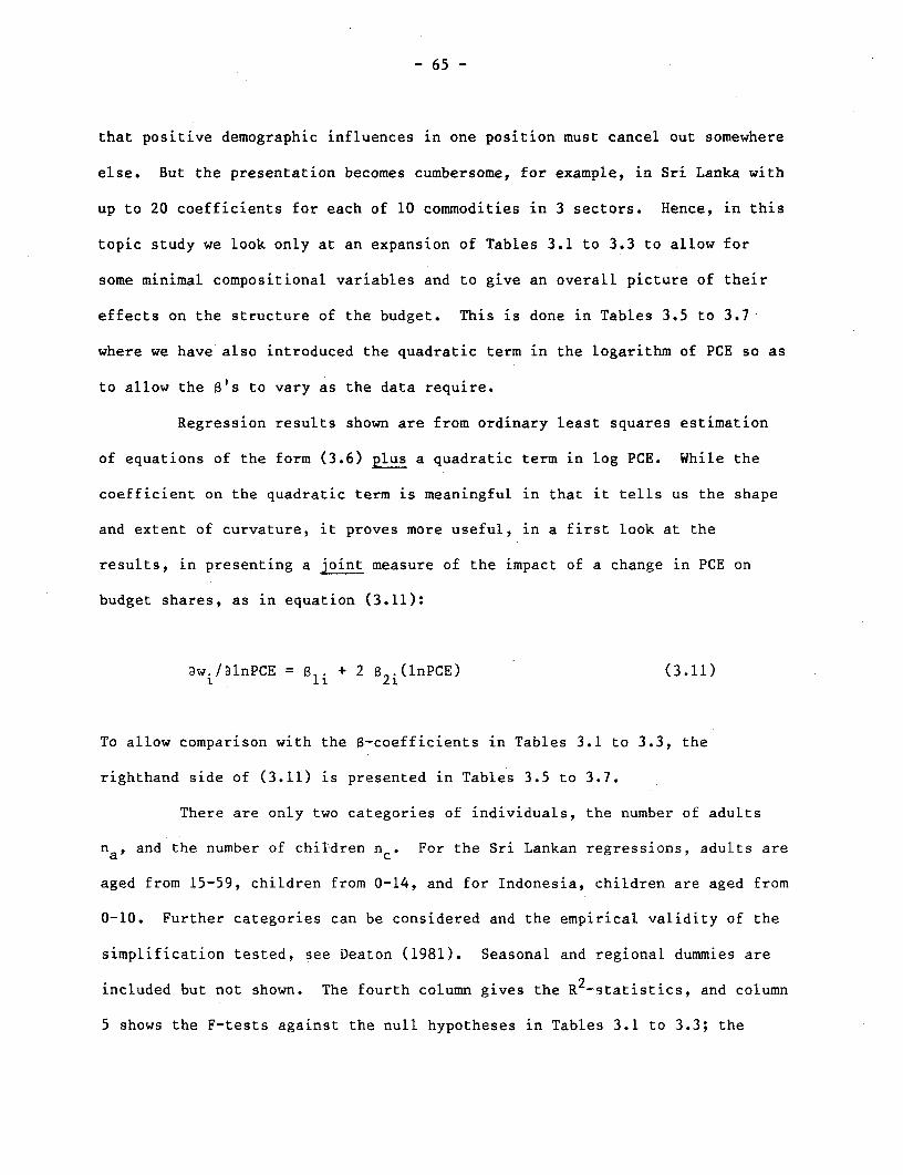
- 65 -
that positive demographic influences in one position must cancel out somewhere
else. But the presentation becomes cumbersome, for example, in Sri Lanka with
up to 20 coefficients for each of 10 commodities in 3 sectors. Hence, in this
topic study we look only at an expansion of Tables 3.1 to 3.3 to allow for
some minimal compositional variables and to give an overall picture of their
effects on the structure of the budget. This is done in Tables 3.5 to 3.7
where we have also introduced the quadratic term in the logarithm of PCE so as
to allow the a's to vary as the data require.
Regression results shown are from ordinary least squares estimation
of equations of the form (3.6) plus a quadratic term in log PCE. While the
coefficient on the quadratic term is meaningful in that it tells us the shape
and extent of curvature, it proves more useful, in a first look at the
results, in presenting a Joint measure of the impact of a change in PCE on
budget shares, as in equation (3.11):
awi/aInPCE =li + 2 2i (lnPCE) (3.11)
To allow comparison with the s-coefficients in Tables 3.1 to 3.3, the
righthand side of (3.11) is presented in Tables 3.5 to 3.7.
There are only two categories of individuals, the number of adults
na, and the number of children nc. For the Sri Lankan regressions, adults are
aged from 15-59, children from 0-14, and for Indonesia, children are aged from
0-10. Further categories can be considered and the empirical validity of the
simplification tested, see Deaton (1981). Seasonal and regional dummies are
included but not shown. The fourth column gives the R2-statistics, and column
5 shows the F-tests against the null hypotheses in Tables 3.1 to 3.3; the

- 66 -
latter is thus a test of the joint significance of the curvature and the
minimal demographic effects. In general, the F-statistics are highly
significant in all sectors of all surveys. The final column is an estimate of
the total expenditure elasticity evaluated at mean budget shares and mean log
PCE.
For all sectors of all three surveys, the elasticity figures differ
from those calculated using (3.2) in that they are lower for necessities
(food, fuel and housing) and higher for luxuries. As Figure 3.5 makes clear,
this is what was to be expected. There, the budget shares predicted with and
without the quadratic term are plotted against log PCE for a necessity (fuel)
and a luxury (household goods) using results from the urban outer islands,
Indonesia 1978. These results are representative of the empirical "fact" that
the expenditure shares of necessities are decreasing at an increasing rate at
average PCE and the shares of luxuries are increasing at an increasing rate.
It is clear from Figure 3.5 that when measured at average PCE and average
share the 6-coefficients estimated using (3.6) are lower for necessities and
higher for luxuries than those estimated with a linear term alone, and the
elasticities will differ correspondingly.
In interpreting these results, some features should be kept in
mind. The R2-statistics may appear to be low, particularly for certain
commodities and on the Sri Lankan estates. As noted above, this simply
reflects the enormous amount of individual variation that is to be expected in
large microeconomic samples. If, for example, the data were to be grouped,
say by income classes, as is often the case, much of the variation would be
removed and the R2-statistics would be very much higher. The overall
significance of the regression can be assessed by F-tests against the null

- 67 -
that the shares are not influenced by any of the variables listed; in all
cases the null is very decisively rejected. As to the significance of
individual coefficients, a common practice is to set to zero those estimates
which are insignificantly different from zero. There is little in the way of
formal justification for such a procedure (see for example, Chapter 3 of Judge
et al., (1980)), but in the present case it has the additional undesirable
feature of destroying the adding-up properties of the estimates which are an
essential feature of explaining the pattern of demand. Columns 1, 2 and 3
each add to zero, but this would not remain true if some equations were re-
estimated with individual coefficients set to zero. Finally, we add the usual
disclaimer about the presence of zero purchases in the calculation of these
estimates. We have rerun regressions excluding zeros, and, in a few cases,
there are substantial differences, not only in parameter levels, but also in
ratios. In particular, conclusions relating to clothing and durables in the
Sri Lankan surveys, and those relating to alcohol, transport and user taxes in
the Indonesian survey, should be treated as highly provisional.
Turning now to the substantive results, Table 3.5 reveals quite
striking patterns associated with the demographic variables for the Sri Lanka
1969-70 survey. We look first at the influence of additional adults, the na
variable. A useful way to interpret-the results is to imagine an already
existing household, of several adults and children, which is joined, on a
permanent basis, by another adult, who brings with him or her a contribution
to household expenditure equal to pre-existing household per capita
expenditure. Such an experiment holds per capita expenditure constant so that
the coefficients of n a effect of the extra individual on the budget shares
once all adjustments have been made. One possibility is that all effects are

TABLE 3.5: QLadratic lPgessicoos with Minjbiml Dep=ic Effects (zero observations in-xuded): Sri lanka 1969-70
Urban RuralPCE* Na Nc R F-test e PCE* Na Nc R2 F-test e
Food -20.04 -0.60 -0.89 .592 74.7 0.68 Food -17.51 -0.58 -0.73 .644 64.0 0.75liquor -0.10 -0.01 -0.03 .117 5.64 1.03 Liquor 0.96 -0.18 -0.02 .031 4.42 1.17Housing 6.53 -0.21 -0.11 .269 51.2 1.53 Housing 0.31 -0.22 -0.47 .114 67.8 1.04Fiel -0.98 -0.16 -0.20 .165 116.0 0.73 Fuel -1.32 -0.21 -0.19 .130 89.8 0.67Clothing 5.01 0.35 0.43 .166 31.0 1.95 Clothing 7.20 0.42 0.72 .178 59.8 2.13Household 1.65 0.08 0.11 .132 29.4 1.44 Household 1.12 0.07 0.09 .083 17.6 1.41Health 1.15 -0.01 0.02 .023 1.84 1.44 Health 1.09 -0.00 0.06 .034 1.36 1.41Transport 0.90 0.05 -0.01 .057 8.50 1.40 Transport 1.51 0.14 0.05 .083 9.70 1.59Recreation 3.20 0.38 0.48 .168 93.0 2.04 Recreation 2.79 0.38 0.33 .121 74.4 2.20Durables 2.47 0.12 0.20 .104 20.4 2.44 Durables 3.03 0.19 0.17 .084 19.6 2.51
Estate 2PCE* Na Nc R F-test e o
Food -15.02 0.08 -0.35 .282 14.2 0.79Liquor 1.52 -0.23 -0.09 .049 6.77 1.22Housing -2.54 -0.48 -0.63 .178 132.0 0.36Fuel -2.32 -0.22 -0.39 .178 66.3 0.31Clothing 11.14 0.51 1.09 .204 28.0 2.36Household 0.19 0.02 -0.02 .035 5.78 1.05Health 1.29 -0.01 0.13 .046 7.60 1.66Transport 0.79 0.02 -0.00 .051 7.38 1.32Recreation 1.88 0.16 0.17 .111 30.5 2.66Durables 2.38 0.14 0.11 .077 13.6 3.11
* The figures shown represent the joint effect of the linear and quadratic ln(PCE) tenns: Bli + 2B2i(lnPCE).Note: Seasonal and regional dummies were included in the regressions.Source: Sri Lanka Socioeconanic Survey, 1969-70.

- 69 -
FIGURE 3.5: Necessities and Luxuries: A Comparison of Budget SharesUrban Outer Islands, Indonesia 1978
4-7~ ~ ~ ~~~~~w = ic6. + Sl 1nPCE
4 6 1 ~~~~+ 62i (lnPCE) 2 +r li r
4.49
4.1
4.0
2000 4000 8000 16000
Predicted fuel share and log POE Per capita expenditure log scale
10.0
7.0
6 .0
5.0
4.0
43inPCE 0 + .ii nPCE
3.0
2.0 + 0,2. (lnPCE)2+ Z yi r
1.0
o
2000 4000 8000 16000
Predicted share of households goods Per capita expenditure log scale
and log POE
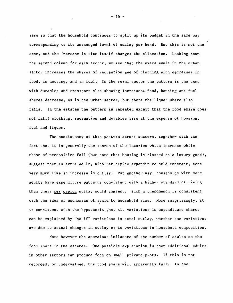
- 70 -
zero so that the household continues to split up its budget in the same way
corresponding to its unchanged level of outlay per head. But this is not the
case, and the increase in size itself changes the allocation. Looking down
the second column for each sector, we see that the extra adult in the urban
sector increases the shares of recreation and of clothing with decreases in
food, in housing, and in fuel. In the rural sector the pattern is the same
with durables and transport also showing increases; food, housing and fuel
shares decrease, as in the urban sector, but there the liquor share also
falls. In the estates the pattern is repeated except that the food share does
not fall; clothing, recreation and durables rise at the expense of housing,
fuel and liquor.
The consistency of this pattern across sectors, together with the
fact that it is generally the shares-of the luxuries which increase while
those of necessities fall (but note that housing is classed as a luxury good),
suggest that an extra adult, with per capita expenditure held constant, acts
very much like an increase in outlay. Put another way, households with more
adults have expenditure patterns consistent with a higher standard of living
than their per capita outlay would suggest. Such a phenomenon is consistent
with the idea of economies of scale to household size. More surprisingly, it
is consistent with the hypothesis that all variations in expenditure shares
can be explained by "as if"-variations in total outlay, whether the variations
are due to actual changes in outlay or to variations in household composition.
Note however the anomalous influence of the number of adults on the
food share in the estates. One possible explanation is that additional adults
in other sectors can produce food on small private plots. If this is not
recorded, or undervalued, the food share will apparently fall. In the

- 71 -
estates, however, there is little or no opportunity for such own-account work
and a much larger proportion of transactions goes through the market.
There is another, alternative explanation of the observed effects of
size. The goods whose shares increase - clothing, durables, and recreational
goods - are typically purchased and consumed on an individual basis. Food,
housing and fuel, by contrast, are provided on a household basis and, indeed,
households are typically defined on the basis of shared accommodation and
food. One might then expect shared goods, some of which have a substantial
overhead or public element, to be more easily spread over an increase in
numbers than private, individual, goods. A cinema ticket gets one person in
to see the movie and one person only, but no house is too small to admit one
more, and no family so poor that it cannot somehow, feed another mouth. Such
an explanation also has the advantage, in light of the empirical results, of
not forcing us to regard housing as a necessity.
If we turn now to the effects of children, as shown in Table 3.5,
they turn out to be qualitatively very similar to those for additional
adults. Once again, families with more children but the same per capita
expenditure spend less of their budget on food, housing and fuel (in all
three sectors) and spend more on clothing, recreation and durables.
Expenditure on household goods also increases in urban, and to some extent, in
rural areas. There is also an interesting positive association between health
expenditures and the presence of children which is apparently confined to the
estates. Broadly speaking, the presence of an additional child (with PCE held
constant) has a larger effect on rearranging the budget than does the presence
of an additional adult. If we follow the first explanation for the size
effects, that of scale economies, this is what we should expect. The PCE

- 72 -
compensation for the child is likely to be overgenerous as compared with that
for the adult, so that the income-like effects of the extra child should be
correspondingly larger. This is sensible enough but what is somewhat
surprising is the relative absence of any strongly specific links between the
presence of children and individual expenditures. It is reasonable to suppose
that additional children bring with them specific needs as well as a general
requirement for more outlay. The latter effect is present, the former is not
obviously detectable except possibly for health expenditure in the estates.
It is conceivable that the specific needs of children will show up at a
greater commodity disaggregation than is adopted here.
In summary, there is a consistent picture across sectors of changes
in household composition acting analogously to changes in total outlay, at
least as a first approximation. Additional adults require additional outlay
to restore expenditure patterns, but less than the average adult; similarly,
and more strongly, for additional children. The presence of extra family
members, whether adults or children, with income compensation to keep per
capita expenditure constant, results in a rise in the shares of luxury goods
such as clothing, durables and recreational expenditures, and a fall in the
shares of necessities such as food, housing and fuel.
The patterns associated with the demographic variables presented in
Table 3.6 for the Sri Lanka 1980-81 survey are generally consistent with those
of the earlier Sri Lankan survey. Again, an extra adult, with per capita
expenditure held constant, decreases the shares of necessities - food (in all
but the estate sector), fuel, and housing (in all but the urban sector) -
while increasing the shares of clothing and recreation. Looking at the
effects of an additional child, we see a similar pattern: an extra child, at
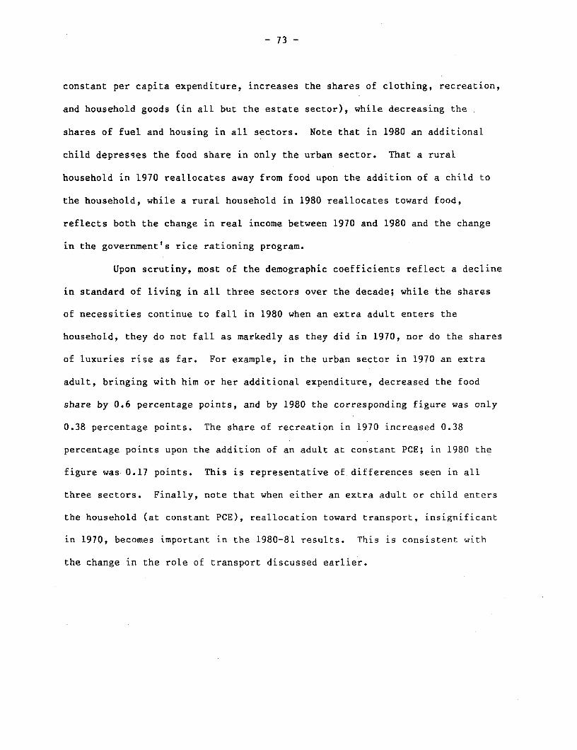
- 73 -
constant per capita expenditure, increases the shares of clothing, recreation,
and household goods (in all but the estate sector), while decreasing the
shares of fuel and housing in all sectors. Note that in 1980 an additional
child depresses the food share in only the urban sector. That a rural
household in 1970 reallocates away from food upon the addition of a child to
the household, while a rural household in 1980 reallocates toward food,
reflects both the change in real income between 1970 and 1980 and the change
in the government's rice rationing program.
Upon scrutiny, most of the demographic coefficients reflect a decline
in standard of living in all three sectors over the decade; while the shares
of necessities continue to fall in 1980 when an extra adult enters the
household, they do not fall as markedly as they did in 1970, nor do the shares
of luxuries rise as far. For example, in the urban sector in 1970 an extra
adult, bringing with him or her additional expenditure, decreased the food
share by 0.6 percentage points, and by 1980 the corresponding figure was only
0.38 percentage points. The share of recreation in 1970 increased 0.38
percentage points upon the addition of an adult at constant PCE; in 1980 the
figure was 0.17 points. This is representative of differences seen in all
three sectors. Finally, note that when either an extra adult or child enters
the household (at constant PCE), reallocation toward transport, insignificant
in 1970, becomes important in the 1980-81 results. This is consistent with
the change in the role of transport discussed earlier.

TABIB 3.6: Qldratic Regressions with Minimal lnpgra4bic Effects (zero observations iwaluded): Sri J.aka 1980-81
Urban RuralPCE* Na Nc R F-test e PCE* Na NC R2 F-test e
Food -14.99 -0.38 -0.65 .558 36.6 0.78 Food -9.69 -0.29 0.06 .296 71.8 0.86Liquor 0.27 -0.18 0.14 .020 4.92 1.07 Liquor 0.77 -0.10 -0.08 .013 2.25 1.17Housing 4.09 0.16 -0.60 .241 24.8 1.56 Housing 0.65 -0.11 -0.38 .071 33.1 1.16Fuel -2.64 -0.27 -0.42 .231 30.3 0.54 Fuel -2.09 -0.43 -0.45 .155 138.0 0.67Clothing 2.09 0.11 0.24 .082 5.15 1.56 Clothing 1.91 0.23 0.09 .075 15.9 1.48Household 2.21 0.06 0.29 .123 11.9 1.69 Household 2.04 0.12 0.20 .102 41.5 1.72Health 1.19 0.05 0.05 .089 6.01 1.45 Health 1.36 -0.01 -0.01 .038 0.17 1.50Transport 4.84 0.24 0.56 .212 20.0 2.11 Transport 3.30 0.29 0.27 .228 157.0 2.09Recreation 2.54 0.17 0.39 .140 11.1 2.17 Recreation 1.63 0.29 0.26 .092 58.9 2.17Coaminication 0.29 0.03 -0.01 .182 23.2 2.31 Communication 0.10 0.02 0.00 .073 29.1 2.28
EstatePCE* Na Nc R2 F-test e
Food -2.75 0.39 0.66 .124 5.83 0.96Liquor 1.49 0.25 -0.22 .078 1.86 1.26Housing -2.86 -0.59 -0.68 .425 76.9 0.07Fuel -2.47 -0.62 -0.47 .197 24.8 0.62Clothing 2.61 0.05 0.30 .072 2.08 1.58Household 0.26 -0.01 -0.01 .074 3.67 1.12Health 0.77 0.15 0.09 .091 1.41 1.40Transport 1.64 0.15 0.12 .136 6.50 2.00Recreation 1.13 0.23 0.20 .070 6.02 2.32Communication 0.06 0.01 0.01 .116 24.1 2.06
* The figures shown represent the joint effect of the linear and quadratic ln(PCE)terms: Bli + 2B2i(1nPCE).
Source: Sri Lanka Socioeconcmic Survey, 1980-81.

- 75 -
Table 3.7 reveals that the broad picture for Sri Lanka also applies
to the Indonesian figures. Both adults and children have negative impacts on
the shares of fuel, housing (except in urban Java, where an extra adult has a
positive impact), and food (except in rural Java, where an extra child has the
opposite effect). As in Sri Lanka, both adults and children bringing their
own PCE raise the shares of household goods, which include education and
health expenditures, transport, and clothing (with the exception of urban
Java, where an additional adult lowers this share). The demographic
coefficients reflect the income disparities between sectors in Indonesia. For
example, an additional adult in the wealthiest sector, urban Java, would
decrease the food share 0.95 percentage points, while that adult in the
poorest sector, the rural Outer Islands, would decrease the share only 0.65
percentage points.

TABLE 3.7: Qndratic Regression vith Minimni Dtmogrp;*ic Effects (zero observatixjs irwludEd) Indonesia 1978
Urban RuralJava Java
PCE* Na Nc R2 F-test e PCE* Na Nc R2 F-test e
Food -12.21 -0.95 -0.06 .417 9.72 0.79 Food -8.99 -0.69 -0.11 .149 10.7 0.87Liquor 0.12 -0.01 -0.00 .005 0.61 2.19 Liquor 0.21 -0.01 0.03 .018 3.66 5.12Housing 6.53 -0.21 -0.11 .269 51.2 1.53 Housing 0.31 -0.22 -0.47 .114 67.8 1.04Tobacco -0.52 -0.25 -0.00 .030 10.8 0.90 Tobacco 1.40 0.15 -0.10 .025 2.19 1.28Housing 6.97 0.33 -0.02 .182 1.73 1.49 Housing 2.22 -0.10 -0.02 .049 0.73 1.62Fuel -2.03 -0.18 -0.50 .262 29.5 0.64 Fuel -3.80 -0.50 -0.99 .143 34.9 0.59Household 2.49 0.94 0.16 .157 30.2 1.32 Household 3.16 0.62 0.33 .088 21.0 1.89Transport 2.80 0.22 0.35 .149 5.62 1.89 Transport 1.22 0.14 0.06 .049 5.07 2.94Clothing 1.56 -0.15 0.11 .044 1.68 1.36 Clothing 4.09 0.23 0.65 .091 8.84 1.78User Taxes 0.91 -0.05 -0.03 .081 4.00 1.57 User Taxes 0.50 0.16 -0.06 .021 7.70 1.39
Urban RuralOuter Is-an Outer Islands
PCE* Na Nc F-test e PCE* Na Nc R F-test e
Fool -10.92 -0.44 -0.58 .221 9.88 0.84 Food -5.64 -0.65 -0.12 .078 5.83 0.93Liquor 0.14 0.01 0.06 .014 6.68 2.43 Liquor 0.34 0.01 0.02 .026 11.9 2.48Tobacco 0.67 -0.26 0.02 .032 15.0 1.11 Tobacco 1.17 0.02 -0.02 .019 23.9 1.21Housing 2.84 -0.18 -0.46 .064 6.17 1.28 Housing 0.09 -0.03 -0.04 .016 10.5 1.02Fuel -0.62 -0.03 -0.19 .017 6.38 0.86 Fuel -0.94 -0.35 -0.68 .051 26.9 0.74Household 3.80 0.62 0.60 .149 53.4 1.74 Household 1.48 0.66 0.30 .085 45.9 1.54Transport 1.61 0.16 0.10 .116 37.0 2.77 Transport 0.21 0.14 0.12 .007 1.77 1.83Clothing 1.85 0.03 0.25 .039 4.42 1.43 User 2.53 0.10 0.40 .041 3.20 1.48User Taxes 0.63 0.09 0.18 .037 15.0 1.68 User Taxes 0.76 0.10 0.01 .016 1.90 1.58
* Te figures sbown represent the joint effect of the linear and quadratic ln(PCE) term: Bli + 2B2i(1nPCE).Source: SUSENAS 1978

- 77 -
Notes for Further Reading
The material of this chapter is the traditional subject matter of the
"analysis of family budgets"; the standard reference remains the book by Prais
and Houthakker (1955). One contribution of that study was to provide a list
of functional forms for Engel curves. These have been widely applied to a
large number of data sets from around the world, see Brown and Deaton (1972)
for a general survey, and Bhattacharyya (1978) for numerous studies for
India. The functional form used in this chapter originates with Holbrook
Working (1943) and so predates Prais and Houthakker, but was not included in
their lists, and so was accorded relatively little attention, at least until
recently, although see Leser (1963, 1976). Yet the Working form satisfies the
adding-up restriction, unlike most of Prais and Houthakker's forms, and is
consistent with the observed nonlinearity in the regression of food
expenditure on total expenditure. It also belongs to a class of utility
consistent models with extremely convenient aggregation properties, see Deaton
and Muellbauer (1980) for a more detailed discussion. The survey paper by
Deaton (1985a) also discusses these matters as well as some of the
developments in Engel curve theory in the last few years.
There are a number of important econometric issues not discussed
above. Most household surveys are stratified, so that while each household
can be regarded as representative of some large number of households in the
population as a whole, the ratios of population to sample households, or
"weights" or sometimes "inflation factors", vary across households. It is
agreed by everyone that when using such data to calculate means, weights
should be applied to each household, so that the sample mean is a consistent
estimate of the population mean, even if the strata are non-homogeneous.

- 78 -
There is much less agreement about the appropriate procedures to be used when
computing a regression. Standard econometric texts either ignore the issue,
or recommend that no weighting be applied, see for example, Klein (1953),
Cramer (1969), or Madalla (1983). The argument is that if the strata are
homogeneous, there is no need to weight and, indeed, weighting will only
decrease the efficiency of the estimation. If the strata are not homogeneous,
the pooled regression does not correspond to any well-defined model, so that
once again, weighting is not the issue. However, it is often difficult to be
sure that all the strata are homogeneous, so that weighting will at least
guarantee that the estimates have limits that are independent of the details
of the stratification scheme, at the price of some efficiency cost when there
is homogeneity. A useful discussion is given by DuMouchel and Duncan (1983)
who point out that the weighted regression estimates are consistent for the
parameters that would be obtained from the population regression. (Note that
it is not clear why this latter should be of interest.)
A second, largely unresolved, issue is how to estimate Engel curves
in the presence of zero expenditures. Zero expenditures are not the same as
other recorded values, if only because they occur much more frequently than
any other single value. Expenditures are also inherently non-negative, so
that zero is not just one more point between minus and plus infinity. The
standard econometric procedure for zeros was suggested by Tobin in 1958, and
is known as Tobin's probit, or (after the Apocryphal prophet) Tobit. This is
a statistical model of censoring, whereby potentially negative values are set
to zero. However, there are problems with the Tobin procedure. Firstly, with
many goods, it is difficult to give a firm theoretical basis to the model; see
for example the discussions in Deaton (1981, 1985), and in Lee and Pitt

- 79 -
(1986). Secondly, it is necessary to model explicitly the fact that zero
purchases appear for more than one reason; the household may never purchase
the good at all, or the household may not purchase the good during the recall
period of the survey. In principle, it is possible to construct models that
take account of all of this, but they are much too complicated to be estimated
even with very high speed computers. Deaton and Irish (1984) provide some
initial and not very successful attempts using a British household survey.
There are also a set of econometric results for somewhat similar models which
suggest that ordinary least squares regression may provide consistent
estimates up to a scale factor, see in particular, Greene (1981), Ruud (1983,
1984), Chung and Goldberger (1984), and Stoker (1984). This is an area where
there are likely to be major developments in the near future. The results for
the Sri Lankan 1969-70 survey are based on the fuller treatment in Deaton
(1981, Essay 1). Similar and more extensive results are given for the 1980-81
survey in Thomas (1985).

- 80 -
CHAPTER IV
MEASURING THE COSTS OF CHILDREN
General Considerations
It is generally accepted that children impose economic costs on their
parents, but there is little general agreement as to how these costs should be
defined or measured. Nevertheless, the issue can hardly be avoided since some
measure of child costs is central to any attempt to make welfare comparisons
between households of different demographic compositions. As a first
approximation, it might be acceptable to count all adults equally, ignoring
any potential economies from sharing in larger households, but it is clearly
unreasonable to count children as having the same needs as adults. The
precise weighting scheme that is used is of more than academic interest, and
is likely to make a significant difference to a number of central policy
questions. Much economic policy in developing countries is concerned with
improving the lot of the poorest members of society, so that the
identification of the poor is of great importance.
Because individuals belong to households, and we typically have no or
few data on allocation within the household, the best that can be done is
usually the identification of poor households. Even if we can agree that
total expenditure is a reasonable approximation to individual welfare, then we
still must account for the variation in demographic composition between
households in moving from household expenditure to some measure of the welfare
of the individuals in it. Now, for most countries, total household
expenditure is positively, but less than proportionately related to household

- 81 -
size. In consequence, use of total household expenditure as a measure of
welfare automatically ensures that small households will be over-represented
among the poor, while using per capita household expenditure will guarantee
that large households are typically poor households. To actually discover
something about the relationship between family size and poverty, as opposed
to assuming a relationship, it is necessary to have some procedure for
defining and measuring the costs of different family sizes, and particularly
the costs of children.
One standard and widely used procedure is to define children, and
sometimes women, as fractions of a male adult according to their nutritional
needs. Various measures of nutritional requirements are available, but the
World Health Organisation (WHO) minimum calorie requirements are probably the
most frequently used. Hence, if a five-year old child "requires" 60 percent
of the calories required by his/her father, and his/her mother "requires" 90
percent of the same amount, then a household consisting of those three persons
would be counted as having 2.5 equivalent male adults. Welfare could then be
measured on a comparable basis across households by calculating total
expenditure per equivalent male adult for each. There is no doubt that this
procedure is a good deal better than doing nothing, and probably at least as
good as comparing households in terms of per capita household expenditure, but
it is unclear that it is correct, or even approximately so. Firstly,
individuals do not consume only food, even in the poorest of countries, and
the calorie based scales do not take into account requirements for other types
of consumption. Of course, if we are only concerned with the poorest of
households, this objection has less force, since food consumption accounts for
70-80 percent of the budget among these groups. Secondly, however, it is very

- 82 -
unclear that the calorie requirements are even relevant to the welfare of the
individuals we are considering. There has been a great deal of dispute as to
whether the WHO or other figures aceurately do measure, or even can in
principle measure, true calorie needs. But even this is not the central
objection, which is that it is quite incorrect to equate welfare with
nutritional status. While adequate nutrition is undoubtedly an important
component of welfare, particularly when incomes are inadequate to ensure
proper nutrition, it makes no sense to claim that it is all of welfare.
Furthermore, the empirical evidence on consumption patterns shows convincingly
that consumers have little respect for nutritional norms, frequently
purchasing so-called luxuries when so-called "basic" needs have not been
met. It seems to us that there is an overwhelming case for accepting
consumers' own evaluations of their needs and preferences, and that the case
is no less strong for very poor undernourished consumers in Sri Lanka or
Indonesia, than it is for materially well-provided individuals in North
America or Western Europe. If so, then the appropriate place to look for a
measure of child costs is in the behavior of households of different
demographic composition, as revealed, for example, in the sort of empirical
evidence discussed above in Chapter III.
A large number of procedures exist for using empirical evidence on
behavior to generate estimates of the costs of children. Some of these are
fairly complex, and can require sophisticated and difficult estimation and
computation, see Deaton and Muellbauer (1980, 1986) for discussion of some of
the details. However, we do not believe that very much is lost by keeping to
the simpler procedures. To early investigators, the problem seemed very
straightforward, and it is worth reviewing their ideas briefly, since the

- 83 -
issues are still very much alive. We all have an intuitive notion of what
sort of costs are associated with the presence of children, so the first
thought is that examination of household budgets ought to lead to their
identification, with total child costs simply being estimated by addition of
the appropriate amounts. For instance, in their classic study of the "money
value of a man", Dublin and Lotka (1930), net out the "input" costs, that is,
the costs of bringing the individual to economic maturity. They begin,
appropriately enough, with "the cost of being born", add on educational costs,
and make allowances for goods that are not child-specific by pro-rating
typical household budgets.
Unfortunately, things are not this simple, and such an attempt is not
likely to be successful in this form. The problem is that the increase in
educational expenditure or whatever is associated with the extra child must be
offset somewhere else in the budget, unless the child is fortunate enough to
bring with it an increase in household resources. Hence, if we could identify
all of the changes in the budget that follow from the arrival of an additional
child (this is what the regression analysis in Chapter III tries to do), and
if we then added up all such changes, we should find that the "'net" figure is
exactly zero. What is needed is some procedure for picking out those changes
in expenditures that are indeed extra costs associated with the child, and
excluding those changes that reflect the sacrifices made by the adults to
accommodate the new expenditures. All of the modern methodologies for
measuring child costs do exactly this either explicitly or implicitly.
Unfortunately the assumptions are more often implicit than explicit, and
different procedures make different assumptions, so that they can yield quite
different answers, even using the same empirical evidence.
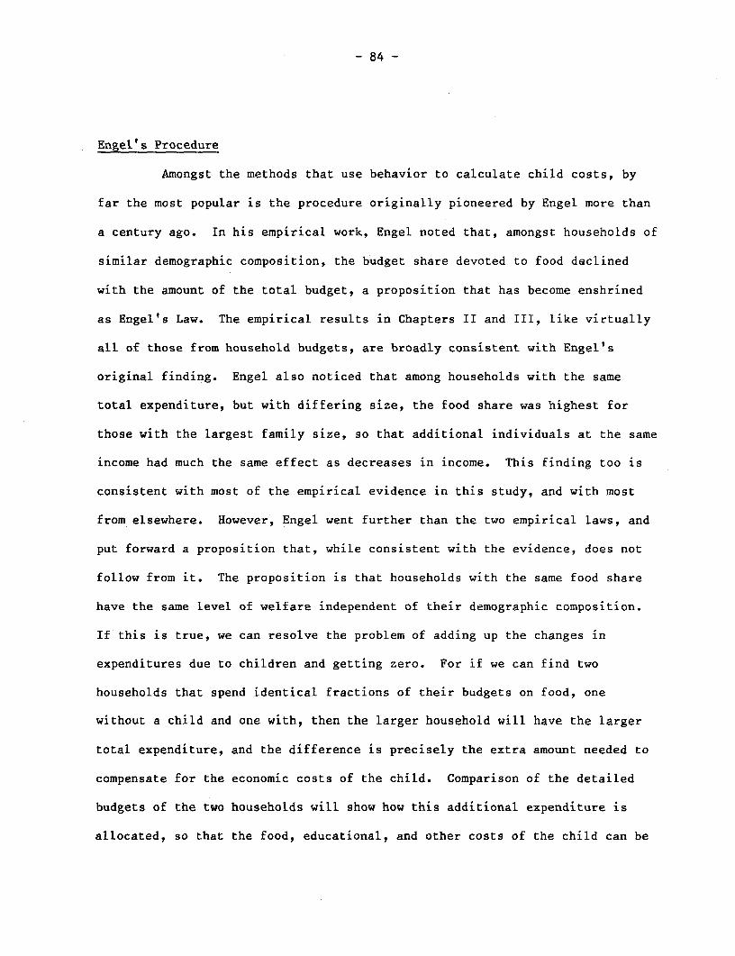
- 84 -
Engel's Procedure
Amongst the methods that use behavior to calculate child costs, by
far the most popular is the procedure originally pioneered by Engel more than
a century ago. In his empirical work, Engel noted that, amongst households of
similar demographic composition, the budget share devoted to food declined
with the amount of the total budget, a proposition that has become enshrined
as Engel's Law. The empirical results in Chapters II and III, like virtually
all of those from household budgets, are broadly consistent with Engel's
original finding. Engel also noticed that among households with the same
total expenditure, but with differing size, the food share was highest for
those with the largest family size, so that additional individuals at the same
income had much the same effect as decreases in income. This finding too is
consistent with most of the empirical evidence in this study, and with most
from elsewhere. However, Engel went further than the two empirical laws, and
put forward a proposition that, while consistent with the evidence, does not
follow from it. The proposition is that households with the same food share
have the same level of welfare independent of their demographic composition.
If this is true, we can resolve the problem of adding up the changes in
expenditures due to children and getting zero. For if we can find two
households that spend identical fractions of their budgets on food, one
without a child and one with, then the larger household will have the larger
total expenditure, and the difference is precisely the extra amount needed to
compensate for the economic costs of the child. Comparison of the detailed
budgets of the two households will show how this additional expenditure is
allocated, so that the food, educational, and other costs of the child can be

- 85 -
identified. In practice, "typical" households from regression analysis are
used rather than individual actual households, but the principle remains the
same. The method also has the great advantage of simplicity. Given an Engel
curve with total expenditure and family size as arguments, the compensations
for additional children require only trivial calculation, or can be read off
from a simple graph.
It is very easy to see the broad outlines of what will happen if
Engel's method is applied to the results in Chapters II and III for the Sri
Lankan and Indonesian surveys. For all three surveys, an excellent
approximation to the effects of demographics on the food-share is given by
including per capita total expenditure as an explanatory variable. In
consequence, to the same degree of approximation, two households will have the
same food share if they have the same level of per capita total expenditure,
no matter how different their compositions. Since food share means welfare
according to Engel, this means that households are compensated for additional
children by keeping their per capita outlay constant, so that, to a first
approximation, children cost the same as adults. In fact, if the additional
demographic terms in the regressions are accounted for, the child costs come
out a little lower, but we still estimate that children cost 80-90 percent as
much as adults, figures that seem implausibly high.
But there are also theoretical reasons for doubting the validity of
Engel's procedure. Note first that Engel's proposition is simply an
assertion; while it is consistent with the empirical evidence, it does not
follow from it. Furthermore, it is a generally implausible assertion.
Consider the following argument, taken from Nicholson (1976): a
household consists of a couple alone, who subsequently have a child. Assume

- 86 -
that the true compensation for the economic costs of the child is known, and
that it is paid to the couple immediately on the birth of the child. By
assumption, the parents are as well off as they were before the birth of their
child, and we can expect them to have a similar consumption pattern. The
child's consumption pattern, however, will generally differ from that of its
parents, and in particular, we may suppose that the child's consumption
pattern will have a greater bias towards food than does that of its parents.
On average, therefore, this perfectly compensated household is spending a
larger proportion of its outlays on food than it did before the birth of the
child. If the household is compensated according to the Engel formula, then
it will have to be given more money so that the food share will be driven down
to its original level. Such a household would therefore be overcompensated.
The amount of money required to keep the food share constant is greater than
that required to compensate the household so that the Engel method generally
overstates the cost of children. Such a theoretical conclusion is certainly
consistent with the evidence given above. On these grounds, we do not
recommend the Engel method for computing child costs; while it is simple, it
is unlikely to give reliable figures, and, as we shall see, there are other
simple methods that make better sense and give more sensible numbers.
Rothbarth's Method
The method we recommend here is a development of the technique first
suggested by Erwin Rothbarth in 1943. The basic idea goes back to that of
Dublin and Lotka, and relies on being able to define certain "adult" goods
that are not directly consumed by children. For these, the presence of
additional children will act like a decrease in income, but otherwise have no
- 87 -
effect. Consider a couple who, before they have children, have a little money
left over after meeting their basic needs which they spend on a weekly visit
to the cinema. The newly arrived child does not go to the cinema, but
nevertheless requires food and clothes which are paid for out of the unchanged
family budget by reductions in the parents expenditure. The parents now visit
the cinema less frequently, they eat rather less well themselves, and they cut
down on their own expenditure on clothing, by making garments last longer, and
by cutting down on items that are not strictly necessary. These cuts are in
response to the need for money to feed and clothe the child; there is no
specific relationship between the consumption given up by the parents and the
child's own consumption. As a consequence, the changes in parents'
consumption are exactly those that would have taken place had there been no
child, only a reduction in their income. In this example, we cannot observe
this for food or for the clothing aggregate, since the reduction in adult
consumption is offset by the new consumption by the child; food and clothing
are "mixed" goods. However, cinema attendance is an adult good, and so is
adult clothing, if such expenditures are distinguished separately in the
data. Therefore, we can identify the reduction in adult expenditures on those
two goods, and if we know from Engel curve analysis what are the income
elasticities of these goods, then we can calculate what income reduction would
have caused the same change in adult expenditure as was caused by the child.
This is the Rothbarth estimate of the cost of the child. Even better, it is
possible to test behavior for the presence of adult goods, at least
partially.
In the above example, since the effect of the demographic change acts
only through the equivalent income change, the ratio of the reduction in adult

- 88 -
clothing expenditure to the marginal propensity to consume adult clothing out
of income should be the same as the ratio of the reduction in cinema
expenditure to the marginal propensity to spend on cinema attendance. For any
group of two or more potential adult goods, such a prediction can be tested.
Alternatively, it is possible to compute ratios for a whole group of goods,
and then to search among them for an empirically satisfactory group of adult
goods. Note however that the empirical results cannot tell us everything. It
is not possible to test a single good for being an adult good, and in any
group of goods, at least one must be selected to be an adult good a priori.
An Empirical Illustration
The details of this procedure will vary from country to country and
from survey to survey, depending on local consumption customs and on the data
that are available. Here we illustrate for the case where detailed data are
available using evidence from a Spanish household survey, and then return to
our examples from Sri Lanka and Indonesia. The Spanish results are taken from
Deaton, Ruiz-Castillo, and Thomas (1985), where the procedures and the survey
are described in much more detail. The Spanish survey (Encuestos de
Presupuestos Familiares 1980-81) is particularly appropriate for this work
because there are 625 separate items of expenditure so that it is possible to
pick out a large number of possible candidates for adult goods. We also
select a number of goods that are potential "child" goods, so that, by analogy
with the adult goods, it is possible to see whether, for those categories, the
presence of additional adults acts like changes in income. Table 4.1 lists
the goods that were chosen for inspection, together with their definitions.
Note that at this stage, we are not committed to any of these as being either

- 89 -
TABLE 4.1: Commodity Shares as a Percentage of Total Expenditureand Fractions of Households Purchasing
FractionMean Share Purchasing Symbol
DETAILED COMMODITIESA. Mainly Adult Goods
Adult Clothing and Footwear 6.11 0.898 ACFMeals and Food Outside theHouse 3.58 0.752 MOUT
Entertainment and Culture 2.72 0.731 ENTCTransport 8.39 0.856 TSPPersonal Care 0.55 0.293 PERC
(a) Unclassified Expenditures 1.61 0.601 NESTobacco and Smoking Devices 1.34 0.639 TOBAlcohol Consumed at Home 1.76 0.712 ALAlcohol Consumed outside Home 1.46 0.611 AOUTHealth 2.27 0.687 HLT
(b) Other Mainly Adult Goods 2.08 0.814 OTHA
B. Mainly Child Goods(c) Baby Goods 0.47 0.178 BABY(d) Regular Children's Goods 2.96 0.616 RCHG(e) Children's Foods (1) 0.55 0.414 CH1(f) Children's Foods (2) 1.21 0.712 CH2
Other Foods 34.68 1.000 FFD(g) Miscellaneous Household Goods 3.66 0.896 CHG(h) Semi-durable Household Goods 1.16 0.423 SDHC
Notes:(a) insurance, gambling, funeral expenses, membership dues and subscriptions, licenses, taxes, and
transfers to public institutions.
(b) stationery excluding school materials, payments for financial services (commission on exchange
transactions), payments for personal services (officials at weddings, funerals).
(c) baby foods, baby clothing, baby furniture, expenditure on day care, and baby carriages and
personal care items.
(d) children's clothing, children's footwear, toys, educational expenses, and children's pocket money.
(e) various foods, including prepared foods with a cereal base, powder items containing cocoa, otherchocolate products, chewing gum and candy bars.
(f) cookies, croissants, donuts, cakes and pies, jams, honey, syrup, ice cream, cocoa and chocolate,frozen and preserved fruits.
(g) current expenditure items: domestic services, bulbs and electrical items, cleaning products,
laundry, toilet paper and other paper products, nails, small accessories.(h) minor capital account items: dishes, pots and pans, coffee machines, hammers and tools, sheets,
blankets, towels and tablecloths.
Source: Deaton, Ruiz-Castillo and Thomas (1985), from Encuestos de Presupuestos Familiares, 1980-81.
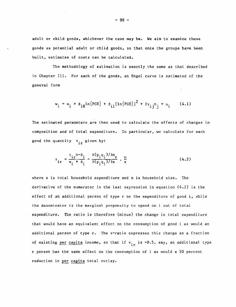
- 90 -
adult or child goods, whichever the case may be. We aim to examine these
goods as potential adult or child goods, so that once the groups have been
built, estimates of costs can be calculated.
The methodology of estimation is exactly the same as that described
in Chapter III. For each of the goods, an Engel curve is estimated of the
general form
i= ai + %Iln{PCEI + a.I[ln{PCE}I2 + ZYi.n, + u. (4.1)
The estimated parameters are then used to calculate the effects of changes in
composition and of total expenditure. In particular, we calculate for each
good the quantity it given by:
y. n-s. a(p.q4l)an'f =i n-f 1= j j1 1n r n (4.2)
ir w. + S i a(pjqj)/ax x
where x is total household expenditure and n is household size. The
derivative of the numerator in the last expression in equation (4.2) is the
effect of an additional person of type r on the expenditure of good i, while
the denominator is the marginal propensity to spend on i out of total
expenditure. The ratio is therefore (minus) the change in total expenditure
that would have an equivalent effect on the consumption of good i as would an
additional person of type r. The i-ratio expresses this change as a fraction
of existing per capita income, so that if it is -0.5, say, an additional type
r person has the same effect on the consumption of i as would a 50 percent
reduction in per capita total outlay.
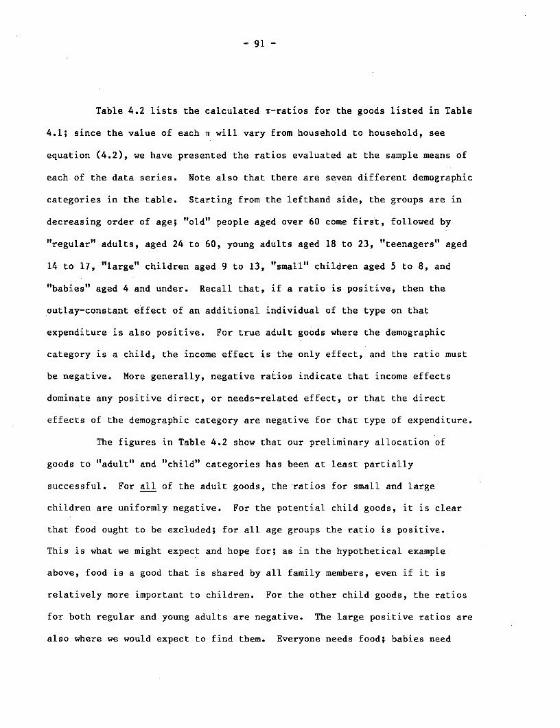
- 91 -
Table 4.2 lists the calculated a-ratios for the goods listed in Table
4.1; since the value of each X will vary from household to household, see
equation (4.2), we have presented the ratios evaluated at the sample means of
each of the data series. Note also that there are seven different demographic
categories in the table. Starting from the lefthand side, the groups are in
decreasing order of age; "old" people aged over 60 come first, followed by
"regular" adults, aged 24 to 60, young adults aged 18 to 23, "teenagers" aged
14 to 17, "large" children aged 9 to 13, "small" children aged 5 to 8, and
"babies" aged 4 and under. Recall that, if a ratio is positive, then the
outlay-constant effect of an additional individual of the type on that
expenditure is also positive. For true adult goods where the demographic
category is a child, the income effect is the only effect, and the ratio must
be negative. More generally, negative ratios indicate that income effects
dominate any positive direct, or needs-related effect, or that the direct
effects of the demographic category are negative for that type of expenditure.
The figures in Table 4.2 show that our preliminary allocation of
goods to "adult" and "child" categories has been at least partially
successful. For all of the adult goods, the ratios for small and large
children are uniformly negative. For the potential child goods, it is clear
that food ought to be excluded; for all age groups the ratio is positive.
This is what we might expect and hope for; as in the hypothetical example
above, food is a good that is shared by all family members, even if it is
relatively more important to children. For the other child goods, the ratios
for both regular and young adults are negative. The large positive ratios are
also where we would expect to find them. Everyone needs food; babies need
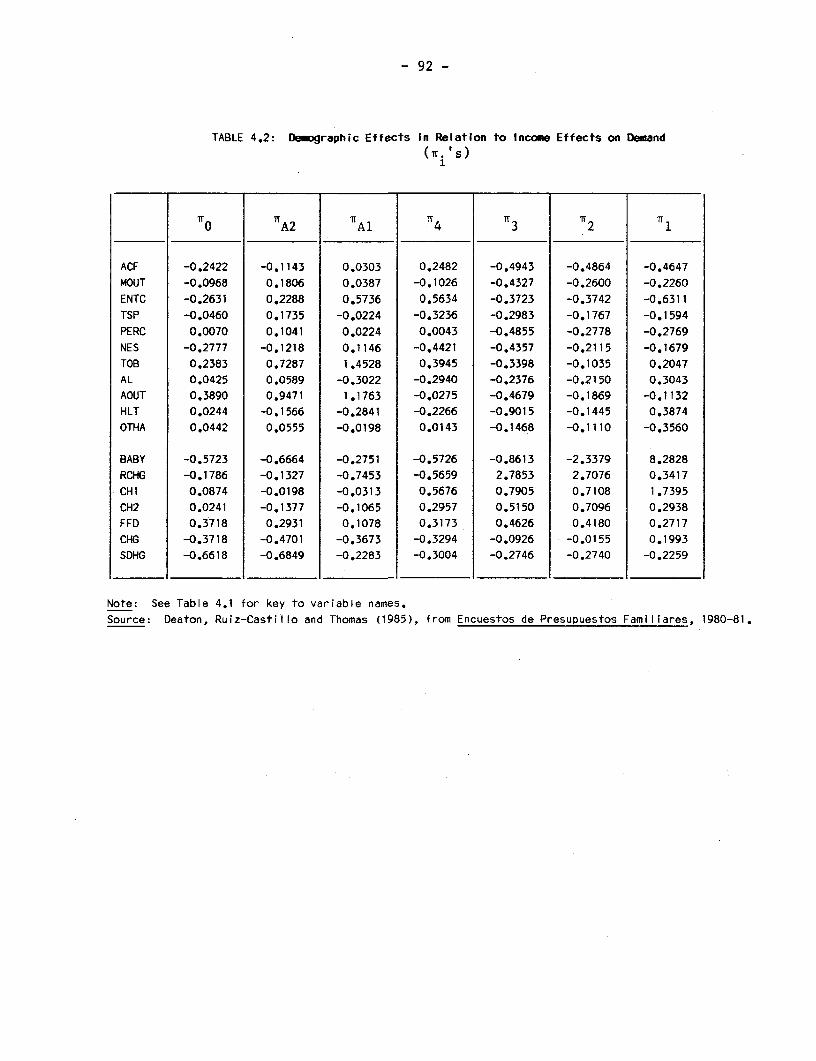
- 92 -
TABLE 4.2: Demographic Effects in Relation to Income Effects on Demand
(Wr. s)
nAl ~ i4 ) t
=~~~~t ° A2 TVAl IT4 73 12 71
ACF -0.2422 -0.1143 0.0303 0.2482 -0.4943 -0.4864 -0.4647
MOUT -0.0968 0.1806 0.0387 -0.1026 -0.4327 -0.2600 -0.2260
ENTC -0.2631 0.2288 0.5736 0.5634 -0.3723 -0.3742 -0.6311
TSP -0.0460 0.1735 -0.0224 -0.3236 -0.2983 -0.1767 -0.1594
PERC 0.0070 0.1041 0.0224 0.0043 -0.4855 -0.2778 -0.2769
NES -0.2777 -0.1218 0.1146 -0.4421 -0.4357 -0.2115 -0.1679
TOB 0.2383 0.7287 1.4528 0.3945 -0.3398 -0.1035 0.2047
AL 0.0425 0.0589 -0.3022 -0.2940 -0.2376 -0.2150 0.3043
AOUT 0.3890 0.9471 1.1763 -0.0275 -0.4679 -0.1869 -0.1132
HLT 0.0244 -0.1566 -0.2841 -0.2266 -0.9015 -0.1445 0.3874
OTHA 0.0442 0.0555 -0.0198 0.0143 -0.1468 -0.1110 -0.3560
BABY -0.5723 -0.6664 -0.2751 -0.5726 -0.8613 -2.3379 8.2828
RCHG -0.1786 -0.1327 -0.7453 -0.5659 2.7853 2.7076 0.3417
CH1 0.0874 -0.0198 -0.0313 0.5676 0.7905 0.7108 1.7395
CH2 0.0241 -0.1377 -0.1065 0.2957 0.5150 0.7096 0.2938
FFD 0.3718 0.2931 0.1078 0.3173 0.4626 0.4180 0.2717
CHG -0.3718 -0.4701 -0.3673 -0.3294 -0.0926 -0.0155 0.1993
SDHG -0.6618 -0.6849 -0.2283 -0.3004 -0.2746 -0.2740 -0.2259
Note: See Table 4.1 for key to variable names.
Source: Deaton, Ruiz-Castillo and Thomas (1985), from Encuestos de Presupuestos Familiares, 1980-81.

- 93 -
baby goods, and children child goods. Young adults have strong effects on
tobacco, on alcohol consumed outside the home, and on entertainment and
culture. Perhaps the most interesting ratios are those for babies on adult
goods. As we should expect, most of the figures are negative, but there are
three exceptions. That for health is not surprising, but there is also
evidence here that the presence of babies is associated with increased
expenditure, presumably by the parents, on alcohol (consumed in the home, not
outside) and on tobacco. This is an effect that is predicted by Barten's
(1964) model of demographic effects; since adult goods do not have to be
shared with children, the presence of children makes adult goods cheaper
relative to mixed goods. Alcohol outside the home would not of course be
rendered cheaper by the presence of children if it is either inconvenient or
expensive to leave them at home. (Barten's is of course not the only
explanation why the presence of infants causes their parents to smoke and
drink more!) As far as we are aware, it is also an effect that typically does
not show up in the data, see for example Atkinson and Stern (1981) for the
United Kingdom and the results above in Chapter III.
Returning to the negative ratios in the Table 4.2, the possibilities
of constructing groups of adult and child goods do not look unpromising.
Looking at the s3 column for adult goods, the average is between -0.3 and
-0.4 with health as a negative outlier (large children depress health
expenditures more than would be expected by what appears to be their income
effect), and with the other category as a positive outlier (conversely). The
same can be said, pari passu, for the next two columns as well as for
the TrA2 and Al columns in the adult good section of the table. Deaton, Ruiz-
Castillo, and Thomas go on to discuss statistical procedures that use these

- 94 -
figures to construct a group of adult goods to be the basis for a measure of
child costs. Various combinations of goods are considered, but once a group
has been defined, costs are calculated by running a regression of the form
(4.1) for the group as a whole, and then calculating the reduction in total
expenditure that would decrease total adult good expenditure by as much as an
uncompensated increase in family size. This can be done for each of the child
groups in Table 4.2, and it was found that, depending on the precise
definition of the group of adult goods, large children were estimated to cost
about one third of an adult, with small children and babies costing about one
quarter. We feel that these figures are much more reasonable than the very
large estimates yielded by the Engel model.
Table 4.3 presents the comparable calculations for the three surveys
discussed in the earlier chapters. Since we do not currently have the same
amount of detail for these surveys as for the Spanish one, the W-ratios are
calculated for the broad groups only. Such groups are of course less likely
to be "pure" adult or child goods. We have also for these surveys re-
estimated the regressions separately for each quartile of per capita
expenditure. This is somewhat more successful for the Sri Lankan surveys than
for the Indonesian one where the Engel curves tend to be unstable across
quartiles. The procedure is designed to pick up possible differences in child
costs between households of different standards of living.

- 95 -
TABLE 4.3: Income Equivalents of an Additional Child Relative toPer Capita Expenditure
Sri Lanka Sri Lanka Indonesia1969-70 1980-81 1978
Food 0.2281 0.1702 0.1117
Alcohol -0.1731 -0.1830 0.1189Tobacco -0.2265
Housing -0.4944 -0.5773 -0.3482
Fuel -0.0572 -0.3310 -0.0379
Clothing -0.1849 -0.2144 -0.1389
Transport -0.3085 -0.2732 -0.3374Communication -0.5394
Household Goods 0.2008 -0.2795 -0.1723
Recreational -0.1349 -0.0994 --
Medical -0.2140 -0.2852 --
User Taxes -- -- -0.1974
Total Non-Food -0.2353 -0.2513 -0.2000
Source: Sri Lanka Socioeconomic Surveys, 1969-70, 1980-81; SUSENAS 1978.
- 96 -
For the Sri Lankan surveys, the ir-ratios are negative except for
food, and for two of the quartiles, for fuel. Hence, additional children act
as would income reductions except for those two goods. The Indonesian story
is similar, though like the Indonesian results in general, the figures are
more erratic and there are a few other positive figures scattered through the
table. Without the commodity detail, we cannot experiment with alternative
definitions of adult goods as we could for Spain. However, transport, alcohol
and tobacco, and clothing are possible categories where the child component is
likely to be relatively small. The ir-ratios for these categories would
suggest an overall average of a quarter to a third, figures that would
translate into a cost per child relative to an adult of 15-20 percent, that
is, somewhat less than the Spanish estimates.
While we find it plausible that the cost of a child relative to an
adult should increase with the level of development, we would not wish to
place too much weight on these figures. We believe that the procedures used
in this chapter are sensible, and we believe that they can usefully and
insightfully be applied elsewhere. However, in the current state of
knowledge, not to say controversy, on these matters, it is better to think of
these methods as yielding orders of magnitudes rather than precise numbers.
The results from the various surveys analyzed here show that adults cut their
own expenditures in response to additional children in the household by an
amount that is consistent with a belief that that children bring additional
needs that are between a third and a sixth of those associated with a typical
adult. Note that this finding, if widely accepted, would imply that
identifying poor people on the basis of household per capita expenditure would
tend to exaggerate the poverty of households that have many children.

- 97 -
Notes for Further Reading
The various procedures for using behavioral evidence as the basis for
estimating child costs are reviewed in Chapter 8 of Deaton and Muellbauer
(1980), see also Pollak and Wales (1982). Apart from the Engel and Rothbarth
procedures that are discussed in this chapter, the most important of the
models are those due to Prais and Houthakker (1955), originally suggested by
Sydenstricker and King (1921), Barten (1964), and Gorman (1976). The Prais-
Houthakker formulation involves a concept of commodity specific adult
equivalents, so that the demand per commodity-specific adult of each good is
linked to the overall resources of the household. Barten's model draws an
elegant analogy between the effects of household composition and the effects
of prices, and so emphasizes the price-like consequences of changes in
household composition. Gorman's model is an extension of Barten's in which
additional individuals bring with them certain fixed costs, as well as
altering "effective" prices in the way suggested by Barten. The Gorman model
is perhaps the one that makes the most theoretical sense, but without making
very special assumptions, both it and the Barten model are complex and
expensive to estimate. Deaton and Muellbauer (1986) show what sort of biases
are involved in using the Rothbarth and Engel procedures when, in fact, the
Gorman model is true. In general, the Engel method is likely to give
estimates that are too small, though the error here is likely to be less
severe.
The Spanish results quoted above are a small part of an extensive
study of demographics on consumption patterns with special reference to the
restrictions implied by the Rothbarth model, see Deaton, Ruiz-Castillo, and
Thomas (1985).

- 98 -
We should note finally that there is a school of thought,
particularly Pollak and Wales (1979) which argues that it is impossible to
infer the costs of children from household budget data. In a sense, this is
true, but no more so than the general proposition that untestable identifying
assumptions are always required before any parameters can be estimated in any
statistical procedure. However, it is certainly the case that much of the
work on measuring child costs has left the identifying assumption
uncomfortably implicit. Different authors have reached different results, not
because their data sets or results were different, but because their
identifying assumptions were different. For example, the Engel measure of
child costs is not an estimate of the same thing as is the Rothbarth estimate,
and it is necessary to decide in advance whether the food share or expenditure
on adult goods is a sensible indicator of adult welfare. We prefer the
latter, and see no grounds for the former. These issues are discussed at
greater length in Deaton and Muellbauer (1986).
The use of nutritional norms, and of the WHO norms in particular, is
discussed by a large number of authors; useful references which contain
further bibliographies are Sukhatme (1977, 1978), Srinivasen (1981), and Sen
(1984). Lipton (1983a and 1983b) discusses the use of calorie based schemes
for the identification of the poor.
- 99 -
CHAPTER V
PRICES AND WELFARE
The prices that consumers pay are the link between their incomes and
their welfare. For producers, market prices also play a role in determining
their incomes. Although household surveys collect only limited information on
prices themselves, survey data on consumption and production provide much of
the information for assessing the link between prices and welfare. Price
indices of the cost-of-living typically use weights from household expenditure
surveys, and the disaggregated data from the surveys allow the construction of
different price indices for different types of households whether
distinguished by occupation, by income, by region, or by demographic
composition. Some of the possibilities are illustrated in this chapter.
Household surveys also provide the basis for an analysis of the effects of
prospective price changes, particularly those arising out of changes in tax or
subsidy policies. Consumption and production data tell us who will benefit
and who will lose under various possible policy changes. They also provide
part of the information necessary for the design of fiscal reform. An
introduction to this kind of analysis is provided below.
Aggregate Price Indices
Economic theory tells us that to obtain a cost-of-living index
comparing one set of prices with another, we must compare the relative costs
of reaching the same welfare level at the two sets of prices. Because price

- 100 -
differences are typically associated with changes in welfare, one of the costs
involved in the comparison is necessarily-a hypothetical one, the calculation
of which requires assumptions about behavior that cannot be checked on cross-
section survey data. However, there are a number of approximations that, in
specific circumstances, are likely to be adequate. The usual formulae, for
comparisons across time, is the Laspeyres price index defined by:
0 1 0 0p = qiPi/ zpqipi (5.1)1 1
where p0. and pi are the prices of good i in periods 0 and 1 and q 0 are the
quantities purchased in the base period. For current purposes, it is more
convenient to rewrite (5.1) in the form:
1
PL Z w° ( i) (5.2)Pi
so that the index is the weighted sum of price relatives, the weights
consisting of the budget shares in the base period.
Depending on the structure of the survey, the Laspeyres formula (5.2)
can be used in a number of ways. Price relatives are typically not collected
as part of the household survey effort. They are collected periodically in
shops and markets rather than in households, and then weighted together using
weights from the most recent available household surveys. In countries where
- 101 -
surveys are frequent, it is possible to smooth the weights by using moving
averages of shares over several years. Usually this is not an option and
indeed, a typical reason for holding a new household survey is that the
weights for the price index are out of date and no longer truly reflect
current spending patterns. It is also important to be aware of the strengths
and the weaknesses of the Laspeyres formula. On the positive side are its
ease of calculation, its relatively close approximation to the "true" cost-of-
living index number over time, and the possibilities for disaggregation (see
below). On the negative side is the fact that the Laspeyres index takes no
account of substitution in response to changes in relative prices, so that the
welfare losses associated with increases in prices tend to be exaggerated.
Over relatively short time periods, this is probably not very serious, but for
longer periods or for comparisons between different countries or regions,
where long-established price differences are related to long-established
differences in consumption patterns, the omission is important and greatly
diminishes the usefulness of the index. Note also that over short time
periods, there are no serious practical problems in measuring the price
relatives (p1/p0); even if the identical commodity cannot be identified, a
close substitute can usually be found. Over longer periods difficulties
become more severe while, over space, insuperable difficulties can often
arise; even within a country, many commodities are available only in specific
locations. For example, "fish" at the coast may be a cheap staple while
"fish" further inland may be a rarely encountered delicacy; it is far from
clear that comparing prices per kilo of a fish (however identified) makes any
sense at all.

- 102 -
As written, the Laspeyres index (5.2) applies to a single household,
although in practice it is invariably used for some group, often for all
households in the economy. A simple average of the Laspeyres indices for each
household is an appropriate method of aggregating. From (5.2), this is what
will automatically be calculated if the average budget shares are applied to
the price relatives (which are, of course, the same for all households). But
frequently Laspeyres indices are not calculated in this way. Instead, the
weights are calculated by dividing society's total expenditure on each good by
the total over all groups. As discussed at the beginning of Chapter II, such
weights are biased towards the expenditure patterns of better-off consumers,
so that their use in a price index also biases the price index to give greater
representation to such households. Prais (1958-9) has called such indices
"plutocratic" price indices and those based on simple averaging (which are
recommended here) "democratic" price indices. Unlike national income data,
containing only aggregate expenditures, household survey data permit
construction of the democratic index.
Disaggregated Price Indices
The Laspeyres formula (5.2) can be applied to any group of
individuals, disaggregated by any criterion. One of the most obvious is to
separate rich from poor consumers since their consumption patterns tend to be
different. In particular, if the relative price of food to manufactured goods
changes, price indices are likely to be quite different for rich versus poor
consumers. For illustration, refer to Table 2.6 showing the distribution of
consumption by deciles in Sri Lanka in 1969-70. Suppose that, over a ten-year
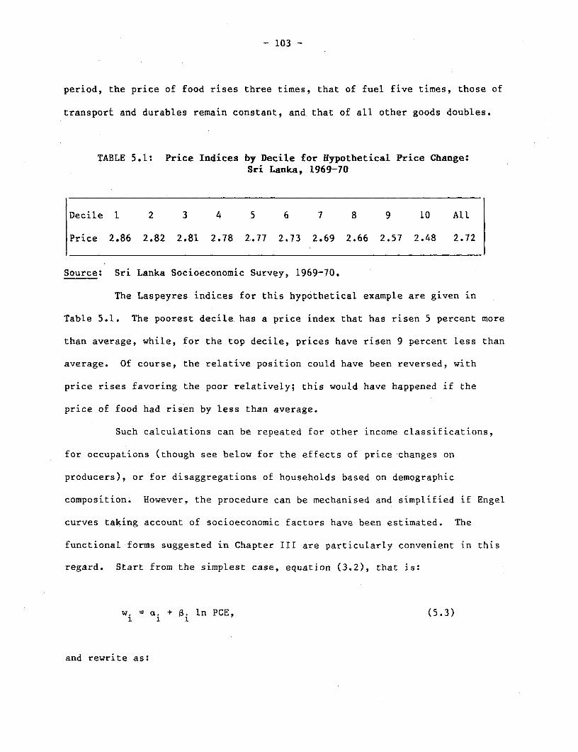
- 103 -
period, the price of food rises three times, that of fuel five times, those of
transport and durables remain constant, and that of all other goods doubles.
TABLE 5.1: Price Indices by Decile for Hypothetical Price Change:Sri Lanka, 1969-70
Decile 1 2 3 4 5 6 7 8 9 10 All
Price 2.86 2.82 2.81 2.78 2.77 2.73 2.69 2.66 2.57 2.48 2.72
Source: Sri Lanka Socioeconomic Survey, 1969-70.
The Laspeyres indices for this hypothetical example are given in
Table 5.1. The poorest decile has a price index that has risen 5 percent more
than average, while, for the top decile, prices have risen 9 percent less than
average. Of course, the relative position could have been reversed, with
price rises favoring the poor relatively; this would have happened if the
price of food had risen by less than average.
Such calculations can be repeated for other income classifications,
for occupations (though see below for the effects of price changes on
producers), or for disaggregations of households based on demographic
composition. However, the procedure can be mechanised and simplified if Engel
curves taking account of socioeconomic factors have been estimated. The
functional forms suggested in Chapter III are particularly convenient in this
regard. Start from the simplest case, equation (3.2), that is:
w= ai + . ln PCE, (5.3)
and rewrite as:
- 104 -
W. a +.' {In PC - lPCE-InPCE} (5.4)1 1 1
where PCE is mean per capita household expenditure and
ai* is ai + .i In PCE. In (5.4), ac* is the budget share of good i
predicted for a household with average PCE. This formula can then be
substituted for the weight in the Laspeyres formula (5.2), so that
1 1*P. P.
= Ea 0) -+ E {ln PCE-InPCE} (5.5)
P i Pi
= pa + PM {ln PCE - ln PCE}. (5.6)
~a admThe quantities P L and PL are referred to as average and marginal price indices
respectively, see Muellbauer (1978) who first suggested this approach; they
are defined by the comparison of (5.5) and (5.6). The average index PL is.a
Laspeyres price index in its own right; it uses the weights for a household at
average PCE and will correspond closely to the single Laspeyres index for the
society as a whole. The marginal index PLm tells us how changes in PCE affect
the cost-of-living. Note that 8i coefficients in (5.4) sum to zero since they
represent the rearrangement of the budget as total outlay changes. P isL
therefore an index whose weights sum to zero, with luxuries having a positive
weight, and necessities a negative weight. Hence, if the price relatives are
such that necessities have become more expensive relative to luxuries (as in
the above example), the marginal index will be negative, and visa versa.

- 105 -
Hence, by employing two sets of weights (the a's and a's), the Engel curve
approach allows any set of price relatives to be used to calculate both the
average Laspeyres index and the distributional impact of the price changes as
summarized in the marginal index. Price changes that give a negative value
to PL can be thought of as "anti-poor", and those with P L positive as "anti-
rich".
In Chapter III, the basic Engel curve specification (5.3) was
compositions, see equation (3.6). Since the numbers of individuals in each
demographic class enter the equation linearly, the approach used above can
also be used to obtain the impact on the Laspeyres index of additional
household members of any particular type. For example, if Yi is the
coefficient linking an individual of type r in the household to the budget
share of good i, then if PCE is held constant, the effect on the Laspeyres
index of replacing an individual of type r by one of type s, is given by
1
APL Yis -Yr ( p) (5.7)L Pi
Prices, Profits, and Consumer Surplus
For some purposes, particularly for the design of government policy,
price indices are clumsy tools since they look at the general consequences of
all price changes. For policies that involve consequential price changes
(taxation and benefit policies, food policy, transport pricing policy, public
projects, and so on), direct assessment of the welfare consequences is
required. The appropriate tools here are those of consumer and producer
surplus. Like index numbers, to which they are closely related, and special
- 106 -
cases apart, consumer and producer surplus measures cannot be evaluated
accurately from household survey data alone. However, there is much that is
relevant in the survey data, certainly enough to make household surveys an
invaluable aid to policy making. In this section, we review some of the
concepts and look at some examples.
Rather than measure the welfare consequences of price changes by
index numbers, it is possible to do so by discovering the amount of money
necessary to compensate the individual. When quantities do not change by
much, or for small price changes, Api say, this is straightforward;
compensation is given by:
C = E q. Ap. (5.8)i 1
It is important to realize that this formula works for producers or
producer/consumers as well as for pure consumers. Since qi is consumption of
good i, production, as negative consumption, must be measured negatively.
This makes sense; if a small farmer is a net producer of rice, an increase in
the price of rice makes him better-off, so that his required compensation is
negative. In general, the qi's in (5.8) are net consumptions, positive if the
unit is a net consumer, and negative if it is a net producer.
The formula (5.8), together with consumption and production data from
a household survey, is in itself a valuable guide to policy. To take a
concrete example, Thailand has a complicated set of policies governing the
sale and distribution of rice, an important element of which is an export tax
which keeps the domestic price of rice well below the world price (about 25
- 107 -
percent below in 1977). An increase in the price of rice might therefore be
thought to be desirable on efficiency grounds; production is likely to be
stimulated and consumers deterred from "inefficient" consumption. It could
also be argued that the price increase will improve distribution by
redistributing real income from urban areas to rural areas where incomes tend
to be lower. These questions can be settled by reference to a household
survey, in this case the 1975/76 Socioeconomic Survey. In the urban areas,
consumers are net consumers of rice and spend between 7 and 9 percent of their
total expenditure, or about 20 percent of total food expenditure, on rice.
Clearly urban consumers will be worse-off as a result of the price change;
those who have the highest budget shares will be the worst affected in
proportion to their resources. Since rice is a necessity, budget shares of
the poor are higher than those of better-off consumers so that any price rise
will worsen the distribution of real income within the urban areas. Turning
to the rural areas, the impact of any price depends on the position of the
household. Those that are not paddy farmers are in the same position as urban
consumers, they are hurt by the change and since they typically spend more of
their budget on rice (18-20 percent), their position would be worsened even
relative to urban consumers. But even among paddy farmers, it turns out that
only relatively large land-owners will benefit by much. Table 5.2, taken from
Trairatvorakul (1984) shows the percentage of paddy-farming households that
are net producers of paddy in relation to farm size.

- 108 -
TABLE 5.2: Farm-Size and Proportion of Net ProducersPaddy-Farmers: Thailand 1975-76
% of Net % of % of Net % OfSize (rai) Producers Sample Size Producers Sample
2 18.2 0.5 30-39 89.4 10.62-4 44.2 7.8 40-49 95.9 5.05-9 66.2 18.6 50-69 94.3 6.310-14 75.6 17.6 70 94.8 3.915-19 80.7 10.920-29 85.0 15.8 Total 7.77 (100)
Source: Trairatvorakul, 1984.
Such partial evidence tends to suggest that an increase in the price
of rice is not likely to be justifiable on distributional grounds alone. Of
course, a full evaluation requires other evidence, particularly on supply and
demand responses to a sizeable price change, as well as on likely changes in
the rural wage in response to the increase in the price of paddy.
In cases where the price change is large, or when the quantities are
very sensitive to price changes, equation (5.8) is unlikely to be a good
approximation to the amount of money required to compensate an individual for
a price change. The problem is that individuals will change their behavior in
response to the change in prices, so that giving them enough money to restore
their original consumption pattern will generally be over-sufficient. A
better approximation to the true compensation is provided by:
0 1 0 1 0 1 0CV Eqi(p. - pi) ½zz (p. - p.)s .(P. - P.) (5.9)
i 1 1 1~~~ i ijJ J
- 109 -
where sij is the substitution effect of an increase in the jth price on the
demand for good i. Clearly, household survey analysis cannot help us measure
these quantities - unless the survey contains genuine regional price variation
- but if only a single price change is being considered, only one price
response is required, and it is often possible to make a reasonable estimate
using off-survey evidence. However, there are alternative approximations that
do not require estimates of price elasticities and that may nevertheless work
well in practice. One useful approach is to specify compensation as a
fraction of original resources rather than as a sum of money; this is more
akin to the index number approach. Define CT, the Tornqvist approximation to
the compensation, by the formula:
log{l + CT/x0} = Zwi(log Pi - log Pi (5.10)
where the w with overbar indicates that the share is the average of the shares
in period 0 and period 1. To interpret this, note that the righthand side is
a weighted average of percentage price changes, where each price change is
weighted according to the importance of the corresponding good in the
budget. The expression is therefore interpretable as the percentage change in
the cost of living. Theleft hand side is approximately CT/x, so that CT is
the fraction of original resources required to make the compensation. The
formal properties of CT are fully discussed by Diewert (1981). The measure
gives an exactly correct measure of compensation under quite general

- 110 -
circumstances, and it requires only limited information. Note, however, that
the calculation does require some estimate of the effects of the policy, since
the demand pattern after the policy change enters into the formula. However,
reasonable conjectures are probably not too hard to come by; for example, Thai
policy makers could almost certainly give a good estimate of the effects of a
10 percent increase in the price of rice on the share of rice expenditure in
urban budgets. Hence the measure CT seems a reasonable compromise between
theoretical accuracy anrd what can be done with the available data.
Designing Taxes and Tax Reform
Many of the considerations of the previous two sections can be
brought together into an analysis of "tax reform." Tax reform analysis is
essentially a cost-benefit analysis of marginal tax changes with the aim of
selecting those directions that will improve the general welfare. Unlike
optimal tax analysis, it does not attempt the more ambitious task of achieving
a welfare optimum. In consequence, a tax reform that appears to be favorable
may weLl be dominated by many other more favorable but unconsidered
alternatives. Put another way, tax reform analysis will by itself not tell us
which of many possible reforms we ought to choose but only whether any given
reform is desirable. However, tax reform analysis has an enormous advantage
over optimum tax analysis in its data requirements; it requires data only on
two current positions of the economy while optimum calculations require data
on the behavior of the economy at the welfare optimum, a point that is in all
likelihood far removed from anything so far experienced. And as we shall see,
even the limited requirements of tax reform analysis are greater than can be
met from a single household survey.

- 111 -
The range for policies that can be considered is extremely wide. The
most obvious are the day to day policy questions of indirect taxes on consumer
goods. In most developing countries, there is a limited range of commodities
that can be directly taxed, but the need for government revenue is often
severe, and it is important for policy makers to have some sensible method for
trading-off the revenue benefits of raising taxes on the one hand with their
consequences for worsening poverty on the other. In many countries, a high
proportion of revenues comes from import and export taxes, and there are taxes
on various forms of intermediate goods, and taxes on production, for example
in the form of procurement policies requiring farmers to sell to the
government some portion of their crop at below market prices. All of these
are ultimately borne by consumers, and the effects of changing rates can be
handled by the general methods outlined below.
The benefits of any tax increase accrue in the form of revenue
increases to the government. While different revenues may be used for
different purposes - for building roads and hospitals, for repaying debt, or
for subsidizing basic needs - a rational government will make some attempt to
satisfy the most urgent of these first, and ultimately to equate the marginal
value to society of different uses of government funds. It is therefore not
unreasonable to consider that the marginal unit of revenue has some sort of
notional worth to society independent of its disposition. Indeed, it is often
convenient to use this value as a numeraire for comparing other uses of funds,
so that, for example, we can consider the question of whether an additional
unit of government revenue is more or less desirable than the same amount of
money in the hands of various other members of society. This, of course, is
- 112 -
the comparison that has to be made in computing the desirability of a tax
change. The change will transfer money from consumers of the good to the
government, and a judgment must be made as to whether the transfer is
worthwhile. Let us examine this in more detail to see where it is that the
information from household surveys is useful.
The revenue that comes from a small tax change depends on the amount
of the good consumed and on the response of that amount to the change in price
induced by the tax. Total consumption will usually be known, particularly if
the good is already being taxed, although surveys could conceivably be useful
if a tax is being considered on a hitherto untaxed commodity. The elasticity
of demand is something that cannot generally be estimated from household
budget data, although there are some surveys where it may be possible to use
regional price variation, see for example the papers by Timmer (1981),
Alderman and Timmer (1979), and Pitt (1983). But it is on estimating the
other side of the account, the effects of taxes on those who pay them, that
the household survey data become central. Clearly, the taxes are borne by
those who consume the good, and are more or less heavily borne depending on
how heavily the good is consumed. Hence, if policy makers wish to calculate
just how the tax will fall, it is essential for them to know just who it is
that consumes the good. For example, it is often argued that it is necessary
to subsidize public transport because of the difficulties faced by the poor in
going to work in some of the larger conurbations in the Third World. This may
be so, but it is important to establish the fact by producing household survey
data showing that the poor do in fact benefit from the subsidies. If the data
show that the poor usually walk to work, then the subsidies cannot usually be
justified on distributional grounds. At this point, middle class interests

- 113 -
are frequently defended by the claim that, "but in our country, everyone is
poor", a claim that is of course irrelevant, for assessing who should bear the
costs of government expenditures.
A policy exercise might therefore be as follows. At the first stage
a list of commodities is drawn up that are either being taxed or could
potentially be so, either directly or indirectly, for example, through an
export tax as in the case of rice in Thailand. For each commodity, policy
advisors calculate an estimate of the tax ch'ange necessary to increase
government revenue by some fixed amount, the same for all commodities, taking
into account both the total consumption of the commodity and its price
elasticity of demand. Household surveys are then used to calculate the
consequences of each of these tax changes for consumers in the economy. One
simple procedure would be to represent the population by a series of
"representative" households each standing in for a particular socioeconomic
group thought to be of relevance to the decision. An obvious possibility
would be to take a representative upper-income urban household, together with
their three rural counterparts. However, there will often be other special
interest groups that need to be represented, if only on political grounds,
while for some specific price changes, rather narrow groups may be affected.
For example, the production of some commodities (fish, woven goods) is often
very geographically concentrated, so that taxes on these goods are likely to
have very specific regional consequences. But given the various
representative households, the effects of raising an equal amount of revenue
through each of the instruments can be calculated in the form of the amount of
money that could be directly taken from the household that would reduce
welfare by as much as the hypothetical tax change. Since tax changes affect

- 114 -
households by increasing prices, the measures that we need are those discussed
in the previous subsection, that is the various compensations, for price
changes.
These are all the data that are required for evaluating any given tax
reform. If achieving the specified increase in revenue by any one tax hurts
all the representative consumers by more than by some other tax, then it is
clearly a good idea to cut that tax, and to gather the revenue by increasing
the other. Of course, the more usual case will be one in which some taxes
hurt some people more than others, with different patterns for the different
ways of raising government revenues. In these cases, policy makers may simply
be able to decide on a policy reform simply by looking at the patterns over
the different types of households, particularly if some favored groups are
singled out by particular instruments. If not, it will generally be necessary
to resort to some sort of distributional weighting scheme, in which
compensations to the various household types are given different social
values. Once these weights are given - and there are many schemes for
calculating them - the weighted compensations can simply be added up and the
tax structure adjusted accordingly.
As most readers will have noticed, these procedures share much with
standard methods in cost-benefit analysis, particularly with the procedures
suggested by Little and Mirrlees (1974), see also Squire and van der Tak
(1975). The models underlying tax reform and cost-benefit analysis are
formally identical, the only difference being that, in cost-benefit analysis,
consideration is given to changes in quantities (a new road, hospital,
factory, or whatever), while in tax reform analysis, we are dealing with

- 115 -
changes in prices. The recent work on tax reform, therefore, is no more than
extension of standard methods of cost-benefit analysis to the examination of
systems of pricing and taxation.
Notes for Further Reading
The index number and consumer surplus theory discussed in this
chapter is standard; a full discussion of the material is given in Chapter 7
of Deaton and Muellbauer (1980) which also contains references to the other
literature. There is much current work on the evaluation of taxes for
developing countries and much of this is collected together in the book edited
by Newbery and Stern (1986).
- 116 -
REFERENCES
Anand, S., and C. Harris. (1985). "Living Standards in Sri Lanka, 1973-81/2: A Partial Analysis of Consumer Finance Survey Data". Washington,D.C., The World Bank (processed).
Atkinson, A.B. (1986). "On the Measurement of Poverty". Econometrica.(forthcoming).
Atkinson, A.B. and N.H. Stern. (1981). "On Labor Supply and CommodityDemands," in A.S. Deaton (ed.), Essays in the Theory and Measurement ofConsumer Behaviour in Honour of Sir Richard Stone. Cambridge: CambridgeUniversity Press, 265-96.
Barten, A.P. (1964). "Family Composition, Prices, and Expenditure Patterns,"in P.E. Hart, G. Mills and J.K. Whitaker (eds), Econometric Analysis forNational Economic Planning. London: Butterworth, 277-92.
Bhalla, S. (1985). "Living Standards in Sri Lanka in the Seventies Mirageand Reality". Washington, D.C., The World Bank, (processed).
Bhattacharya, N. (1963). "On the Effect of Itemization in the Family BudgetSchedule". Calcutta, The Indian Statistical Institute, (processed).
Bhattacharya, N. (1978). "Studies on Consumer Behaviour in India," in, ASurvey of Research in Economics. Vol. 7, Econometrics, New Delhi. Alliedpublishers for the Indian Council of Social Science Research, 176-232.
Brown, J.A.C., and A.S. Deaton. (1972). "Models of Consumer Behaviour: ASurvey". Economic Journal, 82, 1145-1236.
Browning, M.J., A.S. Deaton and M.J. Irish. (1985). "A Profitable Approachto Labor Supply and Commodity Demands over the Life Cycle". Econometrica,53, 503-543.
Caldwell, J.C. (1982). Theory of Fertility Decline. London: Academic Press.
Casley, D.J., and D.A. Lury. (1981). Data Collection in DevelopingCountries. Oxford: Clarendon Press.
Chernichovsky, D., and O.A. Meesook. (1982). "Patterns of Food Consumptionand Nutrition in Indonesia". Washington, D.C., The World Bank,(processed).
Chung, C.-F., and A.S. Goldberger. (1984). "Proportional Projections inLimited Dependent Variable Models". Econometrica, 52, 531-4.
Cramer, J.S. (1969). Empirical Econometrics. Amsterdam, North-Holland.
- 117 -
Deaton, A.S. (1975). "The Structure of Demand in Europe 1920-1970," in C.M.Cippola (ed.), The Fontana Economic History of Europe. London: Collins-Fontana, Vol. 5, 88-131.
Deaton, A.S. (1980). "The Measurement of Welfare: Theory and PracticalGuidelines". The World Bank, Living Standards Measurement Study, WorkingPaper No. 7, Washington, D.C.
Deaton, A.S. (1981). "Three Essays on a Sri Lankan Household Survey". TheWorld Bank, Living Standards Measurement Study, Working Paper No. 11,Washington, D.C.
Deaton, A.S. (1981). "Theoretical and Empirical Approaches to ConsumerDemand Under Rationing," in A.S. Deaton (ed.) Essays in the Theory andMeasurement of Consumer Behaviour in Honour of Sir Richard Stone.Cambridge: Cambridge University Press, 55-72.
Deaton, A.S. (1985a). "Demand Analysis," in Griliches, Z. and M.Intriligator (eds.), The Handbook of Econometrics. Amsterdam: North-Holland, Vol. 3, 1768-1839.
Deaton, A.S. (1985b). "Panel Data from Time-Series of Cross Section,"Journal of Econometrics, 30, 109-126.
Deaton, A.S., and M.J. Irish. (1984). "A Statistical Model for ZeroExpenditures in Household Budgets". Journal of Public Economics, 23, 59-80.
Deaton, A.S., and J. Muellbauer. (1980). Economics and Consumer Behavior.New York: Cambridge University Press.
Deaton, A.S., and J. Muellbauer. (1986). "Measuring Child Costs in PoorCountries". Journal of Political Economy, 94, 720-744.
Deaton, A.S., J. Ruiz-Castillo, and D. Thomas. (1985). "The Influence ofHousehold Composition on Household Expenditure Patterns: Theory andSpanish Evidence". Woodrow Wilson School, Princeton University,processed.
Diewert, W.E. (1981). "The Economic Theory of Index Numbers," in Deaton,A.S. (ed), Essays in the Theory and Measurement of Consumer Behaviour inHonour of Sir Richard Stone. Cambridge: Cambridge University Press, 163-208.
DuMouchel, W.H., and G.J. Duncan. (1983). "Using Sample Survey Weights inMultiple Regression Analyses of Stratified Samples". Journal of theAmerican Statistical Association, 78, 535-43.
Dublin, L.I. and A.J. Lotka. (1930). The Money Value of a Man. New York:Ronald Press. (2nd edition 1947).
- 118 -
Engel, E. (1857). "Die Productions- und Consumtionsverhaltnisse desKonigreichs Sachsen," in E. Engel, (1895), Die Lebenkosten belgischerArbeiter-Familien. Dresden.
Engel, E. (1895). "Die Lebenkosten Belgischer Arbeiter-Familien fruherundjetzt", International Statistical Institute Bulletin, 9, 1-74.
Espenshade, T.J. (1972). "The Price of Children and Socioeconomic Theoriesof Fertility". Population Studies, 26, 207-21.
Espenshade, T.J. (1984). Investing in Children: New Estimates of ParentalExpenditure. Washington, D.C., The Urban Institute Press.
Glewwe, P., and S. Bhalla. (1985). "Unemployment and Wages in Sri Lanka1963-82". Washington, D.C., The World Bank, (processed).
Gorman, W.M. (1976). "Tricks with Utility Functions" in Artis, M. and R.Nobay (eds.), Essays in Economic Analysis. Cambridge: CambridgeUniversity Press.
Greene, W.H. (1981). "On the Asymptotic Bias of the Ordinary Least SquaresEstimator of the Tobit Model". Econometrica, 49, 505-14.
Iyengar, N.S., L.R. Jain, and T.N. Srinivasan. (1968). "Economies of Scalein Household Consumption: A Case Study". Indian Economic Journal,Econometric Annual. 15, 465-77.
Judge, G.C., et al. (1980). The Theory and Practice of Econometrics. NewYork: John Wiley Press.
Klein, L.R. (1953). A Textbook of Econometrics. Evanston, Illinois: Row,Peterson.
Kuznets, S. (1962). "Quantitative Aspects of the Economic Growth ofNations: VII: The Share and Structure of Consumption". EconomicDevelopment and the Cultural Change, 10, 1-92.
Kynch, J., and A.K. Sen. (1983). "Indian Women: Well-Being and Survival".Cambridge Journal of Economics, 7.
Lee, L.F. and M.M. Pitt. (1986). "Specification and Estimation of DemandSystems with Limited Dependent Variables". Econometrica, (forthcoming).
Leser, C.E.V. (1963). "Forms of Engel Functions". Econometrica, 31, 694-703.
Leser, C.E.V. (1976). "Income, Household Size and Price Changes 1953-1973". Oxford Bulletin of Economics and Statistics, 38, 1-10.

- 119 -
Lindert, P.H. (1978). Fertility and Scarcity in America. Princeton:Princeton University Press.
Lindert, P.H. (1980). "Child Costs and Economic Development," in R.A.Easterlin, (ed.), Population and Economic Change in DevelopingCountries. Chicago: University of Chicago Press.for NBER.
Lipton, M. (1983a). "Poverty, Undernutrition, and Hunger". Washington,D.C., World Bank Staff Working Papers No. 597.
Lipton, M. (1983b). "Labor and Poverty". Washington, D.C., World Bank StaffWorking Paper No. 616.
Little, I.M.D., and J.A. Mirrlees. (1974). Project Appraisal and Plann_ngfor Developing Countries. London: Heinemann.
Maddala, G.S. (1983). Limited-dependent and Qualitative Variables inEconometrics. Cambridge and New York: Cambridge University Press.
Muellbauer, J. (1978). "Distributional Aspects of Price Comparisons", inStone, R., and W. Peterson (eds), Econometric Contributions to PublicPolicy. London: MacMillan for the International Economic Association.
Murthy, M N. (1967). Sampling Theory and Methods. Calcutta, StatisticalPublishing Society.
Newbery, D.M.G, and N.H. Stern. (1986). Tax Theory for DevelopingCountries. Washington, D.C., The World Bank.
Nicholson, J.L. (1976). "Appraisal of Different Methods of EstimatingEquivalence Scales and their Results". Review of Income and Wealth, 22,1-11.
Pitt, M.M. (1983). "Food Preferences and Nutrition in rural Bangladesh".Review of Economics and Statistics, 65, 105-14.
Pollak, R.A., and T.J. Wales. (1979). "Welfare Comparisons and EquivalentScales". American Economic Review, 69, 216-21.
Pollak, R.A., and T.J. Wales. (1981). "Demographic Variables in DemandAnalysis". Econometrica, 49, 1533-51.
Prais, S.J. (1958-9). "Whose Cost of Living?" Review of Economic Studies,26, 126-34.
Prais, S.J., and H.S. Houthakker. (1955). The Analysis of Family Budgets.Cambridge: Cambridge University Press.

- 120 -
Pyatt, G., A.R. Roe, et.al. (1977). Social Accounting for DevelopmentPlanning: with Special Reference to Sri Lanka. Cambridge: CambridgeUniversity Press.
Rosenzweig, M.R., and T.P. Schultz. (1982). "Market Opportunities, GeneticEndowments, and Intrafamily Resource Distribution: Child Survival inRural India". American Economic Review, 72.
Rothbarth, E. (1943). "Note on a Method of Determining Equivalent Income forFamilies of Different Composition," Appendix 4 in C. Madge, (ed.), WarTime Pattern of Saving and Spending, Occasional Paper 4, NationalInstitute of Economic and Social Research, London.
Ruud, P.A. (1983). "Sufficient Conditions for the Consistency of MaximumLikelihood Estimation Despite Misspecification of Distribution inMultinomial Discrete Choice Models". Econometrica, 51, 225-28.
Ruud, P.A. (1984). "Consistent Estimation of Limited Dependent VariableModels Despite Misspecification of Distribution". Department ofEconomics, University of California at Berkeley, (processed).
Sen, A.K. (1981). Poverty and Famines: An Essay on Entitlement andDeprivation. Oxford: Clarendon Press.
Sen, A.K. (1984). "Family and Food: Sex Bias in Poverty," in A.K. Sen,Resources, Values, and Development. Cambridge, Mass: Harvard UniversityPress, 346-68.
Squire, L., and H. van der Tak. (1975). Economic Analysis of Projects.Baltimore, Maryland: Johns Hopkins University Press for The World Bank.
Srinivasan, T.N. (1981). "Malnutrition: Some Measurement and PolicyIssues". Journal of Development Economics, 8.
Stigler, G.J. (1954). "The Early History of Empirical Studies of ConsumerBehavior," Journal of Political Economy, 62, 95-113.
Stoker, T. (1984). "Consistent Estimation of Scaled Coefficients". SloanSchool of Management, M.I.T., (processed).
Stone, J.R.N. (1964). The Model in its Environment, Number 5 in A Programmefor Growth. London: Chapman and Hall.
Sukhatme, P.V. (1977). Nutrition and Poverty. New Delhi. IndianAgricultural Research Institute.
Sukhatme, P.V. (1978). "Assessment of Adequacy of Diets at Different IncomeLevels". Economic and Political Weekly, 13 (special issue).

- 121 -
Sydenstricker, E., and W.I. King. (1921). "The Measurement of the RelativeEconomic Status of Families." Quarterly Publication of the AmericanStatistical Association, 17, 842-57.
Thomas, D. (1985). "Essays on the Analysis of Engel Curves in DevelopingCountries". Princeton University, Ph.D. Thesis.
Timmer, C.P. (1981). "Is There Curvature in the Slutsky Matrix?" Review ofEconomic Statistics, 63, 395-402.
Timmer, C.P., and H. Alderman. (1979). "Estimating Consumption Parametersfor Food Policy Analysis". American Journal of Agricultural Economics,61, 982-987.
Timmer, C.P., Falcon, W., and S. Pearson. (1983). Food Policy Analysis.Baltimore: Johns Hopkins University Press.
Tobin, J. (1958). "Estimation of Relationships for Limited DependentVariables". Econometrica, 26, 24-36.
Trairatvorakul, P. (1984). The Effects on Income Distribution and Nutritionof Alternative Rice Price Policies in Thailand. Washington, D.C.,International Food Policy Research Institute.
Visaria, P. (1980). "Poverty and Living Standards in Asia: An Overview ofthe Main Results and Lessons of Selected Household Surveys". Washington,D.C. The World Bank, Living Standards Measurement Study Working Paper No.2.
Willis, R.J. (1982). "The Direction of Intergenerational Transfers andDemographic Transition: The Caldwell Hypothesis Reexamined". Populationand Development Review (Supplement), 8, 207-34.
Working, H. (1943). "Statistical Laws of Family Expenditure". Journal ofthe American Statistical Association, 38, 43-56.

LSMS WORKING PAPER SERIES (continued)
No. 18. Time Use Data and the Living Standards Measurement Study.
No. 19. The Conceptual Basis of Measures of Household Welfare and TheirImplied Survey Data Requirements.
No. 20. Statistical Experimentation for Household Surveys: Two Case Studiesof Hong Kong.
No. 21. The Collection of Price Data for the Measurement of Living Standards.
No. 22. Household Expenditure Surveys: Some Methodological Surveys.
No. 23. Collecting Panel Data in Developing Countries: Does it Make Sense?
No. 24. Measuring and Analyzing Levels of Living in Developing Countries: AnAnnotated Questionnaire.
No. 25. The Demand for Urban Housing in the Ivory Coast.
No. 26. The C8te d'Ivoire Living Standards Survey: Design and Implementation.
No. 27. The Role of Employment and Earnings in Analyzing Levels of Living: AGeneral Methodology with Applications to Malaysia and Thailand.
No. 28. Analysis of Household Expenditures.