Embed Size (px)
Citation preview

Public Debt and Low Interest Rates
By Olivier Blanchard ∗
The lecture focuses on the costs of public debt when safe interestrates are low. I develop four main arguments.First, I show that the current U.S. situation in which safe interestrates are expected to remain below growth rates for a long time,is more the historical norm than the exception. If the future islike the past, this implies that debt rollovers, that is the issuanceof debt without a later increase in taxes may well be feasible. Putbluntly, public debt may have no fiscal cost.Second, even in the absence of fiscal costs, public debt reduces cap-ital accumulation, and may therefore have welfare costs. I showthat welfare costs may be smaller than typically assumed. Thereason is that the safe rate is the risk-adjusted rate of return oncapital. If it is lower than the growth rate, it indicates that therisk-adjusted rate of return to capital is in fact low. The averagerisky rate however also plays a role. I show how both the averagerisky rate and the average safe rate determine welfare outcomes.Third, I look at the evidence on the average risky rate, i.e. theaverage marginal product of capital. While the measured rate ofearnings has been and is still quite high, the evidence from assetmarkets suggests that the marginal product of capital may be lower,with the difference reflecting either mismeasurement of capital orrents. This matters for debt: The lower the marginal product, thelower the welfare cost of debt.Fourth, I discuss a number of arguments against high public debt,and in particular the existence of multiple equilibria where in-vestors believe debt to be risky and, by requiring a risk premium,increase the fiscal burden and make debt effectively more risky.This is a very relevant argument, but it does not have straightfor-ward implications for the appropriate level of debt.My purpose in the lecture is not to argue for more public debt,especially in the current political environment. It is to have aricher discussion of the costs of debt and of fiscal policy than iscurrently the case.
∗ Peterson Institute for International Economics and MIT ([email protected]) AEA Presiden-tial Lecture, to be given in January 2019. Special thanks to Larry Summers for many discussions andmany insights. Thanks for comments, suggestions, and data to Laurence Ball, Simcha Barkai, CharlesBean, Philipp Barrett, Ricardo Caballero, John Campbell, John Cochrane, Carlo Cottarelli, Peter Dia-mond, Stanley Fischer, Francesco Giavazzi, Robert Hall, Patrick Honohan, Anton Korinek, Larry Kot-likoff, Lorenz Kueng, Neil Mehrotra, Jonathan Parker, Thomas Philippon, Jim Poterba, Ricardo Reis,Dmitriy Sergeyev, Jay Shambaugh, Robert Solow, Jaume Ventura, Philippe Weil, Ivan Werning, JerominZettelmeyer, and many of my PIIE colleagues. Thanks for outstanding research assistance to Thomas
1

2 THE AMERICAN ECONOMIC REVIEW MONTH YEAR
I. Introduction
Since 1980, interest rates on U.S. government bonds have steadily decreased.They are now lower than the nominal growth rate, and according to currentforecasts, this is expected to remain the case for the foreseeable future. 10-yearU.S. nominal rates hover around 3%, while forecasts of nominal growth are around4% (2% real growth, 2% inflation). The inequality holds even more strongly inthe other major advanced economies: The 10-year UK nominal rate is 1.3%,compared to forecasts of 10-year nominal growth around 3.6% (1.6% real, 2%inflation). The 10-year Euro nominal rate is 1.2%, compared to forecasts of10-year nominal growth around 3.2% (1.5% real, 2% inflation).1 The 10-yearJapanese nominal rate is 0.1%, compared to forecasts of 10-year nominal growtharound 1.4% (1.0% real, 0.4% inflation).
The question this paper asks is what the implications of such low rates shouldbe for government debt policy. It is an important question for at least two reasons.From a policy viewpoint, whether or not countries should reduce their debt, andby how much, is a central policy issue. From a theory viewpoint, one of pillarsof macroeconomics is the assumption that people, firms, and governments aresubject to intertemporal budget constraints. If the interest rate paid by thegovernment is less the growth rate, then the intertemporal budget constraintfacing the government no longer binds. What the government can and should doin this case is definitely worth exploring.
The paper reaches strong, and, I expect, surprising, conclusions. Put (too)simply, the signal sent by low rates is that not only debt may not have a substantialfiscal cost, but also that it may have limited welfare costs.
Given that these conclusions are at odds with the widespread notion that gov-ernment debt levels are much too high and must urgently be decreased, the paperconsiders several counterarguments, ranging from distortions, to the possibilitythat the future may be very different from the recent past, to multiple equilibria.All these arguments have merit, but they imply a different discussion from thatdominating current discussions of fiscal policy.
The lecture is organized as follows.Section 1 looks at the past behavior of U.S. interest rates and growth rates. It
concludes that the current situation is actually not unusual. While interest rateson public debt vary a lot, they have on average, and in most decades, been lowerthan growth rates. If the future is like the past, the probability that the U.S.government can do a debt rollover, that is issue debt and achieve a decreasingdebt to GDP ratio without ever having to raise taxes later is high.
That debt rollovers may be feasible does not imply however that they are de-sirable. Even if higher debt does not give rise later to a higher tax burden, it
Pellet, Colombe Ladreit, and Gonzalo Huertas. Appendices and data sources: https://bit.ly/2xSSw9O1Different Euro countries have different government bond rates. The 10-year Euro nominal rate
is a composite rate (with changing composition) constructed by the ECB.http://sdw.ecb.europa.eu/quickview.do?SERIES_KEY=143.FM.M.U2.EUR.4F.BB.U2_10Y.YLD

VOL. VOLUME NO. ISSUE DEBT AND RATES 3
still has effects on capital accumulation, and thus on welfare. Whether and whenhigher debt increases or decreases welfare is taken up in Sections 2 and 3.
Section 2 looks at the effects of an intergenerational transfer (a conceptuallysimpler policy than a debt rollover, but a policy that shows most clearly the rel-evant effects at work) in an overlapping generation model with uncertainty. Inthe certainty context analyzed by Diamond (1965), whether such an intergenera-tional transfer from young to old is welfare improving depends on “the” interestrate, which in that model is simply the net marginal product of capital. If theinterest rate is less than the growth rate, then the transfer is welfare improving.Put simply, in that case, a larger intergenerational transfer, or equivalently anincrease in public debt, and thus less capital, is good.
When uncertainty is introduced however, the question becomes what interestrate we should look at to assess welfare effects of such a transfer. Should it bethe average safe rate, i.e. the rate on sovereign bonds (assuming no default risk),or should it be the average marginal product of capital? The answer turns out tobe: Both.
As in the Diamond model, a transfer has two effects on welfare, an effect throughreduced capital accumulation, and an indirect effect, through the induced changein the returns to labor and capital.
The welfare effect through lower capital accumulation depends on the safe rate.It is positive if, on average, the safe rate is less than the growth rate. The intuitivereason is that, in effect, the safe rate is the relevant risk-adjusted rate of returnon capital, thus it is the rate that must be compared to the growth rate.
The welfare effect through the induced change in returns to labor and capitaldepends instead on the (risky) marginal product of capital. It is negative if, onaverage, the marginal product of capital exceeds the growth rate.
Thus, in the current situation where it indeed appears that the safe rate is lessthan the growth rate, but the average marginal product of capital exceeds thegrowth rate, the two effects have opposite signs, and the effect of the transfer onwelfare is ambiguous. The section ends with an approximation which shows mostclearly the relative role of the two rates. The net effect may be positive, if thesafe rate is sufficiently low, and the average marginal product is not too high.
With these results in mind, Section 3 turns to numerical simulations. Peoplelive for two periods, working in the first, and retiring in the second. They haveseparate preferences vis-a-vis intertemporal substitution and risk. This allows tolook at different combinations of risky and safe rates, depending on the degreeof uncertainty and the degree of risk aversion. Production is CES in labor andcapital, and subject to technological shocks: Being able to vary the elasticity ofsubstitution between capital and labor turns out to be important as this elasticitydetermines the strength of the second effect on welfare. There is no technologicalprogress, nor population growth, so the average growth rate is equal to zero.
I show how the welfare effects of a transfer can be positive or negative, andhow they depend in particular on the elasticity of substitution between capital

4 THE AMERICAN ECONOMIC REVIEW MONTH YEAR
and labor. In the case of a linear technology (equivalently, an infinite elasticityof substitution between labor and capital), the rates of return, while random, areindependent of capital accumulation, so that only the first effect is at work, andthe safe rate is the only relevant rate in determining the effect of the transferon welfare. I then show how a lower elasticity of substitution implies a negativesecond effect, leading to an ambiguous welfare outcome.
I then turn to debt and show that a debt rollover differs in two ways froma transfer scheme. First, with respect to feasibility. So long as the safe rateremains less than the growth rate, the ratio of debt to GDP decreases over time;a sequence of adverse shocks may however increase the safe rate sufficiently soas to lead to explosive dynamics, with higher debt increasing the safe rate, andthe higher safe rate in turn increasing debt over time. Second, with respect todesirability: A successful debt rollover can yield positive welfare effects, but lessso than the transfer scheme. The reason is that a debt rollover pays people alower rate of return than the implicit rate in the transfer scheme.
The conclusions, and the welfare effects of debt in Section 3 depend not onlyhow on low the average safe rate is, but also how high the average marginalproduct is. With this in mind, Section 4 returns to the empirical evidence on themarginal product of capital. It focuses on two facts. The first fact is that theratio of the earnings rate of U.S. corporations to their capital at replacement costhas remained high and relatively stable over time. This suggests a high marginalproduct, and thus, other things equal, a higher welfare cost of higher debt. Thesecond fact, however, is that the ratio of the earnings of U.S. corporations to theirmarket value has substantially decreased since the early 1980s. Put another way,Tobin‘s q, which is the ratio of the market value of capital to the value of capitalat replacement cost, has substantially increased. Two potential interpretationsare that capital at replacement cost is poorly measured and does not fully captureintangible capital. The other is that an increasing proportion of earnings comesfrom rents. Both explanations (which are the subject of much current research)imply a lower marginal product for a given measured earnings rate, and thus asmaller welfare cost of debt.
Section 5 goes beyond the formal model and places the results in a broader butinformal discussion of the costs and benefits of public debt.
On one side, the model above has looked at debt issuance used to financetransfers in a full employment economy; this does not do justice to current policydiscussions, which have focused on the role of debt finance to increase demandand output if the economy is in recession, and on the use of debt to finance publicinvestment. This research has concluded that, if the neutral rate of interest is lowand the effective lower bound on interest rates is binding, then there is a strongargument for using fiscal policy to sustain demand. The analysis above suggeststhat, in that very situation, the fiscal and welfare costs of higher debt may belower than has been assumed, reinforcing the case for a fiscal expansion.
On the other side, (at least) three arguments can be raised against the model

VOL. VOLUME NO. ISSUE DEBT AND RATES 5
above and its implications. The first is that the risk premium, and by implicationthe low safe rate relative to the marginal product of capital, may not reflectrisk preferences but distortions, such as financial repression. Traditional financialrepression, i.e. forcing banks to hold government bonds, is gone in the UnitedStates, but one may argue that agency issues within financial institutions orsome forms of financial regulation such as liquidity ratios have similar effects.The second argument is that the future may be very different from the present,and the safe rate may turn out much higher than the past. The third argument isthe possibility of multiple equilibria, that if investors expect the government to beunable to fully repay the debt, they may require a risk premium which makes debtharder to pay back and makes their expectations self-fulfilling. I focus mostly onthis third argument. It is relevant and correct as far as it goes, but it is not clearwhat it implies for the level of public debt: Multiple equilibria typically hold fora large range of debt, and a realistic reduction in debt while debt remains in therange, does not rule out the bad equilibrium.
Section 6 concludes. To be clear: The purpose of the lecture is not to advocatefor higher public debt, but to assess its costs. The hope is that this lecture leadsto a richer discussion of fiscal policy than is currently the case.
II. Interest rates, growth rates, and debt rollovers
Interest rates on U.S. bonds have been and are still unusually low, reflecting inpart the after-effects of the Great Financial Crisis and Quantitative Easing. Thecurrent (December 2018) 1-year T-bill nominal rate is 2.6%, substantially belowthe most recent nominal growth rate, 4.8% (from the second to the third quarter,at annual rates)
The gap between the two is expected to narrow, but most forecasts and mar-ket signals have interest rates remaining below growth rates for a long time tocome. Despite a strong fiscal expansion putting pressure on rates in an economyclose to potential, the current 10-year nominal rate remains around 3%, whileforecasts of nominal growth over the same period are around 4%. Looking at realrates instead, the current 10-year inflation-indexed rate is around 1%, while mostforecasts of real growth over the same period range from 1.5% to 2.5%.2
These forecasts come with substantial uncertainty. Some argue that these lowrates reflect “secular stagnation” forces that are likely to remain relevant forthe foreseeable future3. Others point instead to factors such as aging in advancedeconomies, better social insurance or lower reserve accumulation in emerging mar-kets, which may lead to higher rates in the future (See for example Lukasz and
2Since 1800, 10-year rolling sample averages of U.S. real growth have always been positive, except forone 10-year period, centered in 1930.
3Some point to structurally high saving and low investment, leading to a low equilibrium marginalproduct of capital (for example, Summers (2015), Rachel and Summers (2018). Others point insteadto an increased demand for safe assets, leading to a lower safe rate for a given marginal product (forexample, Caballero, Farhi, and Gourinchas (2017). An interesting attempt to identify the respectiveroles of marginal products, rents, and risk premia is given by Caballero, Farhi and Gourinchas (2017b)

6 THE AMERICAN ECONOMIC REVIEW MONTH YEAR
Smith 2015, Lunsford and West (2018)).Interestingly and importantly however, historically for the United States gov-
ernment, interest rates lower than growth rates have been more the rule than theexception, making the issue of what debt policy should be under this configurationof more than temporary interest.4 .
Evidence on past interest rates and growth rates has been put together by,among others, Shiller (1992) and Jorda et al (2017).5 While the basic conclusionsreached below hold over longer periods, I shall limit myself here to the post-1950period.6 Figure (1) shows the evolution of the nominal GDP growth rate and the1-year Treasury bill rate. Figure (2) shows the evolution of nominal GDP growthrate and the 10-year Treasury bond rate. Together, they have two basic features:
Figure 1. : Nominal growth rate and 1-year T-bill rate
‐4
‐2
0
2
4
6
8
10
12
14
16
Nominal growth rate and 1‐year T‐bill rate
1‐year T‐bill rate nominal growth rate
• On average, over the period, nominal interest rates have been lower thannominal growth rates.7 The 1-year rate has averaged 4.7%, the 10-year ratehas averaged 5.6%, while nominal GDP growth has averaged 6.3%.8
4Two other papers have examined the historical relation between interest rates and growth rates, bothin the United States and abroad, and draw some of the implications for debt dynamics: Mehrotra(2017),and Barrett (2018).
5For evidence going back to the 14th century, see Schmelzing (2018).6There is a striking difference not so much in the level but in the stochastic behavior of rates pre-
and post-1950, with a sharp decrease in volatility post-1950.7Equivalently, if one uses the same deflator, real interest rates have been lower than real growth rates.
Real interest rates are however often computed using CPI inflation rather than the GDP deflator.8Using Shiller’s numbers for interest rates and historical BEA series for GDP, over the longer period

VOL. VOLUME NO. ISSUE DEBT AND RATES 7
Figure 2. : Nominal growth rate and 10-year bond rate
‐4
‐2
0
2
4
6
8
10
12
14
16Nominal growth rate and 10‐year bond rate
nominal 10‐year rate nominal growth rate
• Both the 1-year rate and the 10-year rate were consistently below the growthrate until the disinflation of the early 1980s, Since then, both nominal in-terest rates and nominal growth rates have declined, with rates decliningfaster than growth, even before the Great Financial Crisis. Overall, whilenominal rates vary substantially from year to year, the 1-year rate has beenlower than the growth rate for all decades except for the 1980s. The 10-yearrate has been lower than the growth rate for 4 out of 7 decades.
Given that my focus is on the implications of the joint evolution of interestrates and growth rates for debt dynamics, the next step is to construct a seriesfor the relevant interest rate paid on public debt held by domestic private andforeign investors. I proceed in three steps, first taking into account the maturitycomposition of the debt, second taking into account the tax payments on theinterest received by the holders of public debt, and third, taking into accountJensen’s inequality. (Details of construction are given in appendix A.)9
To take into account maturity, I use information on the average maturity of thedebt held by private investors (that is excluding public institutions and the Fed.)This average maturity went down from 8 years and 4 months in 1950 to 3 yearsand 4 months in 1974, with a mild increase since then to 5 years today.10 Given
1871 to 2018, the 1-year rate has averaged 4.6%, the 10-year rate 4.6% and nominal GDP growth 5.3%.9A more detailed construction of the maturity of the debt held by both private domestic and foreign
investors is given in Hilscher et al (2018).10Fed holdings used to be small, and limited to short maturity T-bills. As a result of quantitative

8 THE AMERICAN ECONOMIC REVIEW MONTH YEAR
this series, I construct a maturity-weighted interest rate as a weighted averageof the 1-year and the 10-year rates using it = αt ∗ i1,t + (1 − αt) ∗ i10,t withαt = (10− average maturity in years)/9.
Many, but not all, holders of government bonds pay taxes on the interest paid,so the interest cost of debt is actually lower than the interest rate itself. There isno direct measure of those taxes, and thus I proceed as follows:1112
I measure the tax rate of the marginal holder by looking at the differencebetween the yield on AAA municipal bonds (which are exempt from Federal taxes)and the yield on a corresponding maturity Treasury bond, for both 1-year and 10-year bonds. Assuming that the marginal investor is indifferent between holdingthe two, the implicit tax rate on 1-year treasuries is given by τ1t = 1 − imt1/i1t,and the implicit tax rate on 10-year Treasuries is given by τ10t = 1− imt10/i10t.
13
The tax rate on 1-year bonds peaks at about 50% in the late 1970s (as inflationand nominal rates are high, leading to high effective tax rates), then goes downclose to zero until the Great Financial Crisis, and has increased slightly since2017. The tax rate on 10-year bonds follows a similar pattern, down from about40% in the early 1980s to close to zero until the Great Financial Crisis, with asmall increase since 2016. 14 Taking into account the maturity structure of thedebt, I then construct an average tax rate in the same way as I constructed theinterest rate above, by constructing τt = αt ∗ τ1,t + (1− αt) ∗ τ10,t
Not all holders of Treasuries pay taxes however. Foreign holders, private andpublic (such as central banks), Federal retirement programs and Fed holdings arenot subject to tax. The proportion of such holders has steadily increased overtime, reflecting the increase in emerging markets’ reserves (in particular China’s),the growth of the Social Security Trust Fund, and more recently, the increasedholdings of the Fed, among other factors. From 15% in 1950, it now accounts for64% today.
Using the maturity adjusted interest rate from above, it, the implicit tax rate,τt, and the proportion of holders likely subject to tax, βt, I construct an “adjustedinterest rate” series according to:
iadj,t = it(1− τt ∗ βt)Its characteristics are shown in Figures (3) and (4). Figure (3) plots the adjusted
easing, they have become larger and skewed towards long maturity bonds, implying a lower maturity ofdebt held by private investors than of total debt.
11For a parallel study, see Feenberg et al (2018).12This is clearly only a partial equilibrium computation. To the extent that debt leads to lower
capital accumulation and thus lower output, other tax revenues may decrease. To the extent howeverthat consumption decreases less, or even increases, the effects depend on how much of taxation is outputbased or consumption based.
13This is an approximation. On the one hand, the average tax rate is likely to exceed this marginalrate. On the other hand, to the extent that municipal bonds are also partially exempt from state taxes,the marginal tax rate may reflect in part the state tax rate in addition to the Federal tax rate.
14The computed tax rates are actually negative during some of the years of the Great Financial Crisis,presumably reflecting the effects of Quantitative Easing. I put them equal to zero for those years

VOL. VOLUME NO. ISSUE DEBT AND RATES 9
rate against the 1-year and the 10-year rates. Figure (4) plots the adjusted taxrate against the nominal growth rate. They yield two conclusions:
Figure 3. : 1-year rate, 10-year rate, and adjusted rate
0
2
4
6
8
10
12
14
16
1‐year rate, 10‐year rate, adjusted rate
10‐year rate 1‐year rate adjusted rate
Figure 4. : Nominal growth rate and adjusted rate
‐4
‐2
0
2
4
6
8
10
12
14
16
Nominal GDP growth and adjusted interest rate
Adjusted rate Nominal GDP growth
• First, over the period, the average adjusted rate has been lower than eitherthe 1-year or the 10-year rates, averaging 3.8% since 1950. This howeverlargely reflects the non neutrality of taxation to inflation in the 1970s and

10 THE AMERICAN ECONOMIC REVIEW MONTH YEAR
1980s, and which is much less of a factor today. Today, the rate is around2.4%.
• Second, over the period, the average adjusted rate has been substantiallylower than the average nominal growth rate, 3.8% versus 6.3%.
The third potential issue is Jensen’s inequality. The dynamics of the ratio ofdebt to GDP are given by:
dt =1 + radj,t
1 + gtdt−1 + xt
where dt is the ratio of debt to GDP (with both variables either in nominal orin real terms if both are deflated by the same deflator), and xt is the ratio of theprimary deficit to GDP (again, with both variables either in nominal or in realterms). The evolution of the ratio depends on the relevant product of interestrates and growth rates (nominal or real) over time.
Given the focus on debt rollovers, that is the issuance of debt without a laterincrease in taxes or reduction in spending, suppose we want to trace debt dynamicsunder the assumption that xt remains equal to zero.15 Suppose that ln[(1 +radj,t)/(1 + gt)] is distributed normally with mean µ and variance σ2. Then, theevolution of the ratio will depend not on expµ but on exp(µ + (1/2)σ2). Wehave seen that, historically, µ was between -1% and -2%. The standard deviationof the log ratio over the same sample was equal to 2.8%, implying a variance of0.08%, thus too small to affect the conclusions substantially. Jensen’s inequalityis thus not an issue here.16
In short, if we assume that the future will be like the past (a big if admittedly),debt rollovers—that is increases in debt without a change in the primary surplus—appear feasible. While the debt ratio may increase for some time due to adverseshocks to growth or positive shocks to the interest rate, it will eventually decreaseover time. In other words, higher debt may not imply a higher fiscal cost.
In this light, it is interesting to do the following counterfactual exercise. Assumethat the debt ratio in year t was what it actually was, but that the primary balancewas equal to zero from then on, so that debt in year t+ n was given by:
dt+n = (i=n∏i=1
1 + radj,t+i1 + gt+i
) dt
15Given that we subtract taxes on interest from interest payments, the primary balance must also becomputed subtracting those tax payments.
16The conclusion is the same if we do not assume log normality, but rather bootstrap from the actualdistribution, which has slightly fatter tails.

VOL. VOLUME NO. ISSUE DEBT AND RATES 11
Figure 5. : Debt dynamics, with zero primary balance, starting in year t.
4060
80100
120
140
index
1950 1960 1970 1980 1990 2000 2010 2020year
Figure 6. : Debt dynamics, with zero primary balance, starting in year t, usingadjusted rate
2040
6080
100
index
1950 1960 1970 1980 1990 2000 2010 2020year
Figures (5) and (6) show what the evolution of the debt ratio would have been,starting at different dates in the past. For convenience, the ratio is normalized to100 at each starting date, so 100 in 1950, 100 in 1960, and so on. Figure (5) usesthe non-tax adjusted rate, Figure (6) uses the tax-adjusted interest rate.
Figure (5) shows how, for each starting date, the debt ratio would eventuallyhave decreased, even in the absence of a primary surplus. The decrease, if startingin the 1950s, 1960s, or 1970s, is quite dramatic. But it also shows that a series ofbad shocks, such as happened in the 1980s, can increase the debt ratio to higher

12 THE AMERICAN ECONOMIC REVIEW MONTH YEAR
levels for a while.Figure (6), which I believe is the more appropriate one, gives an even more
optimistic picture, where the debt ratio rarely would have increased, even in the1980s—the reason being the higher tax revenues associated with inflation duringthat period.
What these figures show is that, historically, debt rollovers would have beenfeasible. Put another way, it shows that the fiscal cost of higher debt would havebeen small, if not zero. This is at striking variance with the current discussionsof fiscal space, which all start from the premise that the interest rate is higherthan the growth rate, implying a tax burden of the debt.
The fact that debt rollovers may be feasible (i.e. that they have not fiscal cost)does not imply however that they are desirable (that they have no welfare cost).This is the topic taken up in the next two sections.
III. Intergenerational transfers and welfare
Debt rollovers are, by essence, non-steady-state phenomena, and have poten-tially complex dynamics and welfare effects. It is useful to start by looking at asimpler policy, namely a transfer from the young to the old (equivalent to pay-as-you-go social security), and then to return to debt and debt rollovers in the nextsection.
The natural set-up to explore the issues is an overlapping generation modelunder uncertainty. The overlapping generation structure implies a real effectof intergenerational transfers or debt, and the presence of uncertainty allows todistinguish between the safe rate and the risky marginal product of capital.17
I proceed in two steps, first briefly reviewing the effects of a transfer under cer-tainty, following Diamond (1965), then extending it to uncertainty. (Derivationsare given in Appendix B)18
Assume that the economy is populated by people who live for two periods,working in the first period, and consuming in both periods. Their utility is givenby:
U = (1− β)U(C1) + βU(C2)
where C1 and C2 are consumption in the first and the second period respectively.
17In this framework, the main effect of intergenerational transfers or debt is to decrease capital ac-cumulation. A number of recent papers have explored the effects of public debt when public debt alsoprovides liquidity services. Aiyagari and McGrattan (1998) for example explore the effects of publicdebt in an economy in which agents cannot borrow and thus engage in precautionary saving; in thatframework, debt relaxes the borrowing constraint and decreases capital accumulation. Angeletos, Collardand Dellas (2016) develop a model where debt provides liquidity. In that model, debt can either crowdout capital, for the same reasons as in Aiyagari and McGrattan, or crowd in capital by increasing theavailable collateral required for investment. These models are obviously very different from the modelpresented here, but all share a focus on the low riskless rate as a signal about the desirability of publicdebt.
18For a nice recent introduction to the logic and implications of the overlapping generation model, seeWeil (2008).

VOL. VOLUME NO. ISSUE DEBT AND RATES 13
(As I limit myself for the moment to looking at the effects of the transfer on utilityin steady state, there is no need for now for a time index.) Their first and secondperiod budget constraints are given by
C1 = W −K −D ; C2 = R K +D
where W is the wage, K is saving (equivalently, next period capital), D is thetransfer from young to old, and R is the rate of return on capital.
I ignore population growth and technological progress, so the growth rate isequal to zero. Production is given by a constant returns production function:
Y = F (K,N)
It is convenient to normalize labor to 1, so Y = F (K, 1). Both factors are paidtheir marginal product.
The first order condition for utility maximisation is given by:
(1− β) U ′(C1) = βR U ′(C2)
The effect of a small increase in the transfer D on utility is given by:
dU = [−(1− β)U ′(C1) + βU ′(C2)] dD + [(1− β)U ′(C1) dW + βKU ′(C2) dR]
The first term in brackets, call it dUa, represents the partial equilibrium, di-rect, effect of the transfer; the second term, call it dUb, represents the generalequilibrium effect of the transfer through the induced change in wages and ratesof return.
Consider the first term, the effect of debt on utility given labor and capitalprices. Using the first-order condition gives:
(1) dUa = [β(−R U ′(C2) + U ′(C2))] dD = β(1−R)U ′(C2) dD
So, if R < 1 (the case known as “dynamic inefficiency”), then, ignoring theother term, a small increase in the transfer increases welfare. The explanation isstraightforward: If R < 1, the transfer gives a higher rate of return to savers thandoes capital.
Take the second term, the effect of debt on utility through the changes in Wand R. An increase in debt decreases capital and thus decreases the wage andincreases the rate of return on capital. What is the effect on welfare?
Using the factor price frontier relation dW/dR = −K/N ,or equivalently dW =

14 THE AMERICAN ECONOMIC REVIEW MONTH YEAR
−KdR (given that N = 1), rewrite this second term as:
dUb = −[(1− β)U ′(C1)− βU ′(C2)]K dR
Using the first order condition for utility maximization gives:
dUb = −[β(R− 1)U ′(C2)]K dR
So, if R < 1 then, just like the first term, a small increase in the transferincreases welfare (as the lower capital stock leads to an increase in the interestrate). The explanation is again straightforward: Given the factor price frontierrelation, the decrease in the capital leads to an equal decrease in income in thefirst period and increase in income in the second period. If R < 1, this is moreattractive than what capital provides, and thus increases welfare.
Using the definition of the elasticity of substitution η ≡ (FKFN )/FKNF , thedefinition of the share of labor, α = FN/F , and the relation between secondderivatives of the production function, FNK = −KFKK , this second term can berewritten as:
(2) dUb = [β(1/η)α][(R− 1)U ′(C2)]R dK
Note the following two implications of equations (1) and (2):
• The sign of the two effects depends on R−1. If R < 1, the a decrease in capi-tal accumulation increases utility. In other words, if the marginal product isless than the growth rate (which here is equal to zero), an intergenerationaltransfer has a positive effect on welfare in steady state.
• The strength of the second effect depends on the elasticity of substitutionη. If for example η = ∞ so the production function is linear and capitalaccumulation has no effect on either wages or rates of return to capital, thissecond effect is equal to zero.
So far, I just replicated the analysis in Diamond.19 Now introduce uncertaintyin production, so the marginal product of capital is uncertain. If people are riskaverse, the average safe rate will be less than the average marginal product ofcapital. The basic question becomes:
What is the relevant rate we should look at for welfare purposes? Put loosely,is it the average marginal product of capital ER, or is it the average safe rateERf , or it is some other rate altogether?
The model is the same as before, except for the introduction of uncertainty:
19Formally, Diamond looks at the effects of a change in debt rather than a transfer. But, undercertainty and in steady state, the two are equivalent.

VOL. VOLUME NO. ISSUE DEBT AND RATES 15
People born at time t have expected utility given by: (I now need time subscriptsas the steady state is stochastic):
U = (1− β)U(C1,t) + βEU(C2,t+1)
Their budget constraints are given by
C1t = Wt −Kt −D ;C2t+1 = Rt+1 Kt +D
Production is given by a constant returns production function
Yt = AtF (Kt−1, N)
where N = 1 and At is stochastic. (The capital at time t reflects the saving ofthe young at time t− 1, thus the timing convention).
At time t, the first order condition for utility maximization is given by:
(1− β) U ′(C1,t) = βE[Rt+1 U′(C2,t+1)]
We can now define a shadow safe rate Rft+1, which must satisfy:
Rft+1E[U ′(C2,t+1] = E[Rt+1 U′(C2,t+1)]
Now consider a small increase in D on utility at time t:
dUt = [−(1−β)U ′(C1,t)+βEU′(C2,t+1)] dD+[(1−β)U ′(C1,t) dWt+βKtE(U ′(C2,t+1) dRt+1)]
As before, the first term in brackets, call it dUat, reflects the partial equilibrium,direct, effect of the transfer, the second term, call it dUbt, reflects the generalequilibrium effect of the transfer through the change in wages and rates of returnto capital.
Take the first term, the effect of debt on utility given prices. Using the firstorder condition gives:
dUat = [−βE[Rt+1 U′(C2,t+1)] + βE[U ′(C2,t+1)]] dD
So:
(3) dUat = β(1−Rft+1)EU ′(C2,t+1) dD
So, to determine the sign effect of the transfer on welfare through this first
channel, the relevant rate is indeed the safe rate. In any period in which Rft+1

16 THE AMERICAN ECONOMIC REVIEW MONTH YEAR
is less than one, the transfer is welfare improving.
The explanation why the safe rate is what matters is straightforward and im-portant: The safe rate is, in effect, the risk-adjusted rate of return on capital.20
The intergenerational transfer gives a higher rate of return to people than therisk-adjusted rate of return on capital.
Take the second term, the effect of the transfer on utility through prices:
dUbt = (1− β)U ′(C1,t) dWt + βE[U ′(C2,t+1) Kt dRt+1]
Or using the factor price frontier relation:
dUbt = (1− β)U ′(C1,t) Kt−1dRt + βE[U ′(C2,t+1) Kt dRt+1]
In general, this term will depend both on dKt−1 (which affects dWt) and on dKt
(which affects dRt+1). If we evaluate it at Kt = Kt−1 = K and dKt = dKt+1 =dK, it can be rewritten, using the same steps as in the certainty case, as:
(4) dUbt = [β1
ηα] E[(Rt+1 −
Rt+1
Rt)U ′(C2,t+1)]RtdK
Or:
(5) dUbt = [β1
ηα
1
Rt] E[(Rt+1U
′(C2,t+1)](Rt − 1)dK
Thus the relevant rate in assessing the sign of the welfare effect of the transferthrough this second term is the risky rate, the marginal product of capital.If Rt is less than one, the implicit transfer due to the change in input pricesincreases utility. If Rt is greater than one, the implicit transfer decreases utility.
The explanation why it is the risky rate that matters is simple. Capital yieldsa rate of return of Rt+1. The change in prices due to the decrease in capitalrepresents an implicit transfer with rate of return of Rt+1/Rt. Thus, whether theimplicit transfer increases or decreases utility depends on whether Rt is less orgreater than one.
Putting the two sets of results together: If the safe rate is less than one, andthe risky rate is greater than one—the configuration which appears to be relevanttoday—the two terms now work in opposite directions: The first term implies thatan increase in debt increases welfare. The second term implies that an increasein debt instead decreases welfare. Both rates are thus relevant.
20The relevance of the safe rate in assessing the return to capital accumulation was one of themes inSummers (1990).

VOL. VOLUME NO. ISSUE DEBT AND RATES 17
To get a sense of relative magnitudes of the two effects, and therefore whichone is likely to dominate, the following approximation is useful: Evaluate the twoterms at the average values of the safe and the risky rates, to get:
dU/dD = [(1− ERf )− (1/η) α ERf (ER− 1)] βE[U ′(C2)](−dK/dD)
so that:
(6) sign dU ≡ sign [(1− ERf )− (1/η)αERf (−dK/dD)(ER− 1)]
where, from the accumulation equation, we have the following approximation:21
dK/dD ≈ − 1
1− βα(1/η)ER
Note that, if the production is linear, and so η =∞, the second term in equation(6) is equal to zero, and the only rate that matters is ERf . Thus, if ERf is lessthan one, a higher transfer increases welfare. As the elasticity of substitutionbecomes smaller, the price effect becomes stronger, and, eventually, the welfareeffect changes sign and becomes negative.
In the Cobb-Douglas case, using the fact that ER ≈ (1 − α)/(αβ), (the ap-proximation comes from ignoring Jensen’s inequality) the equation reduces to thesimpler formula:
(7) sign dU ≡ sign [(1− ERf ER)]
Suppose that the average annual safe rate is 2% lower than the growth rate, sothat ERf , the gross rate of return over a unit period—say 25 years—is 0.9825 =0.6, then the welfare effect of a small increase in the transfer is positive if ER isless than 1.66, or equivalently, if the average annual marginal product is less than2% above the growth rate.22
Short of a much richer model, it is difficult to know how reliable these roughcomputations are as a guide to reality. The model surely overstates the degree of
21This is an approximation in two ways. It ignores uncertainty and assumes that the direct effect ofthe transfer on saving is 1 for 1, which is an approximation.
22Note that the economy we are looking at may be dynamically efficient in the sense of Zilcha (1991).Zilcha defined dynamic efficiency as the condition that there is no reallocation such that consumptionof either the young or the old can be increased in at least one state of nature and one period, and notdecreased in any other; the motivation for the definition is that it makes the condition independentof preferences. He then showed that in a stationary economy, a necessary and sufficient condition fordynamic inefficiency is that E lnR > 0. What the argument in the text has shown is that an intergener-ational transfer can be welfare improving even if the Zilcha condition holds: As we saw, expected utilitycan increase even if the average risky rate is large, so long as the safe rate is low enough. The reallocationis such that consumption indeed decreases in some states, yet expected utility is increased.

18 THE AMERICAN ECONOMIC REVIEW MONTH YEAR
non Ricardian equivalence: Debt in this economy is (nearly fully) net wealth, evenif Rf is greater than one, and the government must levy taxes to pay the interestto keep the debt constant. The assumption that capital and labor are equallyrisky may not be right: Holding claims to capital, i.e. shares, involves price risk,which is absent from the model, as capital fully depreciates within a period; onthe other hand, labor income, in the absence of insurance against unemployment,can also be very risky. Another restrictive assumption of the model is that theeconomy is closed: In an open economy, the effect on capital is likely to be smaller,with changes in public debt being partly reflected in increases in external debt.I return to the issue when discussing debt (rather than intertemporal transfers)later. Be this as it may, the analysis suggests that the welfare effects of a transfermay not necessarily be adverse, or, if adverse, may not be very large.
IV. Simulations. Transfers, debt, and debt rollovers
To get a more concrete picture, and turn to the effects of debt and debt rolloversrequires going to simulations.23 Within the structure of the model above, I makethe following specific assumptions: (Derivations and details of simulation aregiven in Appendix C.)
I think of each of the two periods of life as equal to twenty five years. Given therole of risk aversion in determining the gap between the average safe and riskyrates, I want to separate the elasticity of substitution across the two periods oflife and the degree of risk aversion. Thus I assume that utility has an Epstein-Zin-Weil representation of the form (Epstein and Zin(2013), Weil (1990)):
(1− β) lnC1,t + β1
1− γlnE(C1−γ
2,t+1)
The log-log specification implies that the intertemporal elasticity of substitutionis equal to 1. The coefficient of relative risk aversion is given by γ.
As the strength of the second effect above depends on the elasticity of sub-stitution between capital and labor, I assume that production is characterizedby a constant elasticity of substitution production function, with multiplicativeuncertainty:
Yt = At (bKρt−1 + (1− b)Nρ)
1/ρ= At(bK
ρt−1 + (1− b))1/ρ
where At is white noise and is distributed log normally, with lnAt ∼ N (µ;σ2)and ρ = (η − 1)/η, where η is the elasticity of substitution. When η =∞, ρ = 1and the production function is linear.
Finally, I assume that, in addition to the wage, the young receive a non-stochastic endowment, X. Given that the wage follows a log normal distribution
23One can make some progress analytically, and, in Blanchard and Weil (1990), we did characterizethe behavior of debt at the margin (that is, taking the no-debt prices as given), for a number of differentutility and production functions and different incomplete market structures. We only focused on debtdynamics however, and not on the normative implications.

VOL. VOLUME NO. ISSUE DEBT AND RATES 19
and thus can be arbitrarily small, such an endowment is needed to make sure thatthe deterministic transfer from the young to the old is always feasible, no matterwhat the realization of W .24 I assume that the endowment is equal to 100% ofthe average wage.
Given the results in the previous section, I calibrate the model so as to fita set of values for the average safe rate and the average risky rate. I consideraverage net annual risky rates (marginal products of capital) minus the growthrate (here equal to zero) between 0% and 4%. These imply values of the average25-year gross risky rate, ER, between 1.00 and 2.66. I consider average net annualsafe rates minus the growth rate between -2% and 1%; these imply values of theaverage 25-year gross safe rate, ERf , between 0.60 and 1.28.
I choose some of the coefficients a priori. I choose b (which is equal to thecapital share in the Cobb-Douglas case) to be 1/3. For reasons explained below,I choose the annual value of σa to be a high 4% a year, which implies a value ofσ of
√25 ∗ 4% = 0.20.
Because the strength of the second effect above depends on the elasticity ofsubstitution, I consider two different values of η, η = ∞ which corresponds tothe linear production function case, and in which the price effects of lower capitalaccumulation are equal to zero, and η = 1, the Cobb-Douglas case, which isgenerally seen as a good description of the production function in the mediumrun.
The central parameters are, on the one hand, β and µ, and on the other, γ.
The parameters β and µ determine (together with σ, which plays a minor role)the average level of capital accumulation and thus the average marginal productof capital—the average risky rate. In general, both parameters matter. In thelinear production case however, the marginal product of capital is independent ofthe level of capital, and thus depends only on µ; thus, I choose µ to fit the averagevalue of the marginal product. In the Cobb-Douglas case, the marginal productof capital is instead independent of µ and depends only on β; thus I choose β tofit the average value of the marginal product of capital.
The parameter γ determines, together with σ the spread between the risky rateand the safe rate. In the absence of transfers, the following relation holds betweenthe two rates:
lnRft+1 − lnERt+1 = −γσ2
This relation implies however that the model suffers from a strong case of theequity premium puzzle (see for example Kocherlakota (1996)). If we think of σas the standard deviation of TFP growth, and assume that, in the data, TFPgrowth is a random walk (with drift), this implies an annual value of σa of about
24Alternatively, a lower bound on the wage distribution will work as well. But this would implychoosing another distribution than the log normal assumption.

20 THE AMERICAN ECONOMIC REVIEW MONTH YEAR
2%, equivalently a value of σ over the 25-year period of 10%, and thus a value ofσ2 of 1%. Thus, if we think of the annual risk premium as, say, 5%, which impliesa value of the right hand side of 1.22, this implies a value of γ, the coefficientof relative risk aversion of 122, which is clearly implausible. One of the reasonswhy the model fails so badly is the symmetry in the degree of uncertainty facinglabor and capital, and the absence of price risk associated with holding shares(as capital fully depreciates within the 25-year period). If we take instead σ toreflect the standard deviation of annual rates of stock returns, say 15% a year (itshistorical mean), and assume stock returns to be uncorrelated over time, then σover the 25-year period is equal to 75%, implying values of γ around 2.5. Thereis no satisfactory way to deal with the issue within the model, so as an uneasycompromise, I choose σ = 20%. Given σ, γ is determined for each pair of averagerisky and safe rates.25
I then consider the effects on steady state welfare of an intergenerational trans-fer. The basic results are summarized in the four figures below.
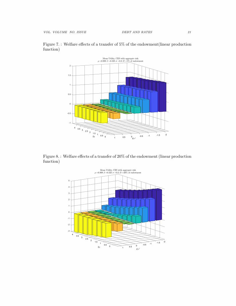
Figure (7) shows the welfare effects of a small transfer (5% of the endowment)on welfare for the different combinations of the safe and the risky rates (reported,for convenience, as net rates at annual values, rather than as gross rates at 25-yearvalues), in the case where η =∞ and, thus, production is linear. In this case, thederivation above showed that, to a first order, only the safe rate mattered. Thisis confirmed visually in the figure. Welfare increases if the safe rate is negative(more precisely, if it is below the growth rate, here equal to zero), no matter whatthe average risky rate.
Figure (8) looks at a larger transfer (20% of the endowment), again in thelinear production case. For a given ERf , a larger ER leads to a smaller welfareincrease if welfare increases, and to a larger welfare decrease if welfare decreases.The reason is as follows: As the size of the transfer increases, second periodincome becomes less risky, so the risk premium decreases, increasing ERf forgiven average ER. In the limit, a transfer which led people to save nothing incapital would eliminate uncertainty about second period income, and thus wouldlead to ERf = ER. The larger ER, the faster ERf increases with a large transfer;for ER high enough , and for D large enough, ERf becomes larger than one, andthe transfer becomes welfare decreasing.
In other words, even if the transfer has no effect on the average rate of returnto capital, it reduces the risk premium, and thus increases the safe rate. At somepoint, the safe rate becomes positive, and the transfer has a negative effect onwelfare.
Figures (9) and (10) do the same, but now for the Cobb-Douglas case. They
25Extending the model to allow uncertainty to differ for capital and labor is difficult to do (except forthe case where production is linear and one can easily capture capital or labor augmenting technologyshocks. In this case, the qualitative discussion of the previous section remains relevant.)
VOL. VOLUME NO. ISSUE DEBT AND RATES 21
Figure 7. : Welfare effects of a transfer of 5% of the endowment(linear productionfunction)
-1
-0.5
0
0.5
1
1.5
2
4 3.5 3 2.5 2 1.5 1 -2 -1.50.5 -1 -0.50 0 0.5 1
Figure 8. : Welfare effects of a transfer of 20% of the endowment (linear productionfunction)
-3
-2
-1
0
1
2
3
4
4
5
3.53
2.52 -2 1.5 -1.51 -1 -0.50.5 0 0 0.5 1

22 THE AMERICAN ECONOMIC REVIEW MONTH YEAR
yield the following conclusions: Both effects are now at work, and both ratesmatter: A lower safe rate makes it more likely that the transfer will increasewelfare; a higher risky rate makes it less likely. For a small transfer (5% of theendowment), a safe rate 1% lower than the growth rate leads to an increase inwelfare so long the risky rate is less than 1.7% above the growth rate. A safe rate2% lower than the growth rate leads to an increase in welfare so long the riskyrate is less than 3.3% above the growth rate. For a larger transfer, (10% of theendowment), which increases the average Rf closer to 1, the trade-off becomesless attractive. For welfare to increase, a safe rate of 2% less than the growth raterequires that the risky rate be less than 2.3% above the growth rate; a safe rateof 1% below the growth rate requires that the risky rate be less than 1.5% abovethe growth rate.
Figure 9. : Welfare effects of a transfer of 5% of the endowment. Cobb-Douglas
I have so far focused on intergenerational transfers, such as we might observein a pay-as-you-go system. Building on this analysis, I now turn to debt, andproceed in two steps, first looking at the effects of a permanent increase in debt,then at debt rollovers.
Suppose the government increases the level of debt and maintains it at thishigher level forever. Depending on the value of the safe rate every period, this
may require either issuing new debt when Rft < 1 and distributing the proceeds as

VOL. VOLUME NO. ISSUE DEBT AND RATES 23
Figure 10. : Welfare effets of a transfer of 10% of the endowment. Cobb Douglas
benefits, or retiring debt, when Rft > 1 and financing it through taxes. FollowingDiamond, assume that benefits and taxes are paid to, or levied on, the young. Inthis case, the budget constraints faced by somebody born at time t are given by:
C1t = (Wt +X + (1−Rft )D)− (Kt +D) = Wt +X −Kt −DRft
C2t+1 = Rt+1Kt +DRft+1
So, a constant level of debt can be thought of as an intergenerational transfer,with a small difference relative to the case developed earlier. The difference is
that a generation born at t makes a net transfer of DRft when young, and receives,
when old, a net transfer of DRft+1, as opposed to the one-for-one transfer studied
earlier. Under certainty, in steady state, Rf is constant and the two are equal.Under uncertainty, the variation about the terms of the intertemporal transferimply a smaller increase in welfare than in the transfer case. Otherwise, theconclusions are very similar.
This is a good place to discuss informally a possible extension of the closedeconomy model, and allow the economy to be open. Start by thinking of a smallopen economy which takes Rf as given and unaffected by its actions. In this case,if Rf is less than one, an increase in debt unambiguously increases welfare. Thereason is that capital accumulation is unaffected, with the increase in debt fully

24 THE AMERICAN ECONOMIC REVIEW MONTH YEAR
reflected in an increase in external debt, so the second effect characterized aboveis absent. In the case of a large economy such as the United States, an increasein debt will lead to both an increase in external debt and a decrease in capitalaccumulation. While the decrease in capital accumulation is the same as abovefor the world as a whole, the decrease in U.S. capital accumulation is smaller thanin the closed economy. Thus, the second effect is smaller; if it were adverse, itis less adverse. This may not be the end of the story however: Other countriessuffer from the decrease in capital accumulation, leading possibly to a change intheir own debt policy. I leave this extension to another paper.
Let me finally turn to the effects of a debt rollover, where the government, afterhaving issued debt and distributed the proceeds as transfers, does not raise taxesthereafter, and lets debt dynamics play out.
The government issues debt D0. Unless the debt rollover fails, there are neithertaxes nor subsidies after the initial issuance and associated transfer. The budgetconstraints faced by somebody born at time t are thus given by:
C1t = Wt +X − (Kt +Dt)
C2t+1 = Rt+1Kt +DtRft+1
And debt follows:
Dt = Rft Dt−1
First, consider sustainability. Even if debt decreases in expected value over
time, a debt rollover, i.e. the issuance of debt paying Rft , may fail with positive
probability. A sequence of realizations of Rft > 1 may increase debt to the levelwhere Rf becomes larger than one and remains so, leading to a debt explosion.At some point, an adjustment will have to take place, either through default, orthrough an increase in taxes. The probability of such a sequence over a long butfinite period of time is however likely to be small if Rf starts far below 1.26
This is shown in Figure (11), which plots 1000 stochastic paths of debt evolu-tions, under the assumption that the production function is linear, and Figure(12), under the assumption that the production function is Cobb-Douglas. Inboth cases, the initial increase in debt is equal to 16.875%) of the endowment.27
26In my paper with Philippe Weil (Blanchard Weil 2001), we characterized debt dynamics, based onan epsilon increase in debt, under different assumptions about technology and preferences. We showedin particular that, under the assumptions in the text, debt would follow a random walk with negativedrift. We did not however look at welfare implications.
27These may seem small relative to actual debt to income ratios. But note two things. The first isthat, in the United States, the riskless rate is lower than the growth rate despite an existing debt to GDPratio around 80%, and a large intergenerational transfer system. If there were no public debt nor socialsecurity system at all, presumably all interest rates, including the riskless rate would be substantially

VOL. VOLUME NO. ISSUE DEBT AND RATES 25
The underlying parameters in both cases are calibrated so as to fit values of ERand ERf absent debt corresponding to -1% for the annual safe rate, and 2% forthe annual risky rate.
Failure is defined as the point where the safe rate becomes sufficiently largeand positive (so that the probability that debt does not explode becomes verysmall—depending on the unlikely realisation of successive large positive shockswhich would take the safe rate back below the growth rate); rather arbitrarily,I choose the threshold to be 1% at an annual rate. If the debt rollover fails, Iassume, again arbitrarily and too strongly, that all debt is paid back through atax on the young. This exaggerates the effect of failure on the young in thatperiod, but is simplest to capture.28
In the linear case, the higher debt and lower capital accumulation have no effecton the risky rate, and a limited effect on the safe rate, and all paths show decliningdebt. Four periods out (100 years), all of them have lower debt than at the start.
Figure 11. : Linear production function. Debt evolutions under a debt rolloverD0= 16.875% of endowment
en
-�rn
,,......_
<l)l:f:.... '----'
� en
�
Debt Share of Savings, Linear OLG With Uncertainty ER=2% ERf=-1% initdebt =16.875%
20 -----,f--------------'--------------'-------------'---------------+-
18
16
14
12
10
8
6-----,f-------------�------------r---------------r---------------+-
0 25 50 Time (year)
75 100
In the Cobb-Douglas case, with the same values of ER and ERf absent debt,bad shocks, which lead to higher debt and lower capital accumulation, lead toincreases in the risky rate, and by implication, larger increases in the safe rate.The result is that, for the same sequence of shocks, now 5% of paths, fail over the
lower (a point made by Larry Summers (2018)). Thus, the simulation is in effect looking at additionalincreases in debt, starting from current levels. The second point is that, under a debt rollover, currentdebt is not offset by future taxes, and thus is fully net wealth. This in turn implies that it has a strongeffect on capital accumulation, and in turn on both the risky and the safe rate.
28An alternative assumption would be default on the debt. This however would make public debtrisky throughout, and lead to a much harder problem to solve.

26 THE AMERICAN ECONOMIC REVIEW MONTH YEAR
Figure 12. : Cobb-Douglas production function. Debt evolutions under a debtrollover D0= 16.875% of endowment
)
Debt Share of Savings, CB OLG With Uncertainty ER=2% ERf=-1% initdebt =16.875%
35 -----,f--------------'--------------'-------------'---------------+-
en b.() � -�rn
4-. o-
30
25
<l) i:f: 20 .... '----'
� en
..., ..0 <l)
� 15
10
5-----,f-------------�------------r--------------r---------------+-
0 25 50 Time (year)
75 100
first four periods—100 years if we take a period to be 25 years. The failing pathsare represented in red.
Second, consider welfare effects: Relative to a pay-as-you-go scheme, debtrollovers are much less attractive. Remember the two effects of an intergener-ational transfer. The first comes from the fact that people receive a rate of return
of 1 on the transfer, a rate which is typically higher than Rft . In a debt rollover,
they receive a rate of return of only Rft−1, which is typically less than one. Atthe margin, they are indifferent to holding debt or capital. There is still an infra-marginal effect, a consumer surplus (taking the form of a less risky portfolio, andthus less risky second period consumption), but the positive effect on welfare issmaller than in the straight transfer scheme. The second effect, due to the changein wages and rate of return on capital, is still present, so the net effect on welfare,while less persistent as debt decreases over time, is more likely to be negative.
These effects is shown in Figures (13) and (14), which show the average welfareeffects of successful and unsuccessful debt rollovers, for the linear and the Cobb-Douglas case.
In the linear case, debt rollovers typically do not fail and welfare is increasedthroughout. For the generation receiving the initial transfer associated with debtissuance, the effect is clearly positive and large. For later generations, while theyare, at the margin, indifferent between holding safe debt or risky capital, theinframarginal gains (from a less risky portfolio) imply slightly larger utility. Butthe welfare gain is small (equal initially to about 0.3% and decreasing over time),

VOL. VOLUME NO. ISSUE DEBT AND RATES 27
Figure 13. : Linear production function. Welfare effects of a debt rollover D0=18% of endowment
Linear OLG With Uncertainty ER=2% ERf=-1% initdebt =16.875%
0.6 -t-------------�------------�------------�------------+--
0.5
0.4
� �0.3
0.1
0-t-------------�------------�------------�------------+--
0 25 50 Time (year)
75 100
Figure 14. : Cobb-Douglas production function. Welfare effects of a debt rolloverD0= 18% of endowment
...., i; "::)
0 '"' (1) " 0 ...., (1)
,;:;...., o:l -
al � ...
;,:.;...., �....,;:I
(1) ...., o:l b.O (1) '"' b.O b.O
�
CB OLG With Uncertainty ER=2% ERf=-1% initdebt =16.875%
4-----,f--------------'--------------'-------------'---------------+-
2
0
-2
-4
-6
-8
-10 -----,f--------------r--------------r--------------r---------------+-
0 25 50 Time (year)
75 100

28 THE AMERICAN ECONOMIC REVIEW MONTH YEAR
compared to the initial welfare effect on the young from the initial transfer, (7%).In the Cobb-Douglas case however, this positive effect is more than offset by
the price effect, and while welfare still goes up for the first generation (by 3%),it is typically negative thereafter. In the case of successful debt rollovers, theaverage adverse welfare cost decreases as debt decreases over time. In the caseof unsuccessful rollovers, the adjustment implies a larger welfare loss when ithappens.29
If we take the Cobb-Douglas example to be more representative, are these Ponzigambles—as Ball, Elmendorf and Mankiw have called them—worth it from awelfare viewpoint? This clearly depends on the relative weight the policy makerputs on the utility of different generations. If the social discount factor it usesis close to one, then debt rollovers under the conditions underlying the CobbDouglas simulation are likely to be unappealing, and lead to a social welfare loss.If it is less than one, the large initial increase in utility may well dominate theaverage utility loss later.
V. Earnings versus marginal products
The argument developed in the previous two sections showed that the welfareeffects of an intergenerational transfer—or an increase in debt, or a debt rollover—depend both on how low the average safe rate and how high the average marginalproduct of capital are relative to growth rate. The higher the average marginalproduct of capital, for a given safe rate, the more adverse the effects of thetransfer. In the simulations above (reiterating the caveats about how seriouslyone should take the quantitative implications of that model), the welfare effectsof an average marginal product far above the growth rate typically dominatedthe effects of an average safe slightly below the growth rate, implying a negativeeffect of the transfer (or of debt) on welfare.
Such a configuration would seem to be the empirically relevant one. Look atFigure (15). The blue line gives the evolution of the ratio of pre-tax earnings ofU.S. non-financial corporations, defined as their net operating surplus, to theircapital stock measured at replacement cost, since 1950. Note that, while thisearnings rate declined from 1950 to the late 1970s, it has been rather stable sincethen, around a high 10%, so 6 to 8% above the growth rate. (see Appendix E fordetails of construction and sources)
Look at the red line however. The line gives the evolution of the ratio of thesame earnings series, now to the market value of the same firms, constructed asthe sum of the market value of equity plus other liabilities minus financial assets.Note how it has declined since the early 1980s, going down from roughly 10%
29Note that the cost of adjustments when a rollover is unsuccessful increases over time. This is becausethe average value of debt, conditional on exceeding the threshold, increases for some time. Initially, onlya few paths reach the threshold, and the value of debt, conditional on exceeding the threshold, is veryclose to the threshold. As the distribution becomes wider, the value of debt, conditional on crossingthe threshold increases. As the distribution eventually stabilizes, the welfare cost also stabilizes. In thesimulation, this happens after approximately 6 periods, or 150 years.

VOL. VOLUME NO. ISSUE DEBT AND RATES 29
then to about 5% today. Put another way, the ratio of the market value of firmsto their measured capital at replacement cost, known as Tobin’s q, has roughlydoubled since the early 1980s, going roughly from 1 to 2.
There are two ways of explaining this diverging evolution; both have implica-tions for the average marginal product of capital, and, as result, for the welfareeffects of debt.30 Both have been and are the subject of much research, triggeredby an apparent increase in markups and concentration in many sectors of the U.S.economy (e.g. DeLoecker and Eeckhout (2017), Gutierrez and Philippon (2017),Philippon (2018), Barkai (2018), Farhi and Gouriou (2018).)
0
2
4
6
8
10
12
14
16
18
1950 1953 1956 1959 1962 1965 1968 1971 1974 1977 1980 1983 1986 1989 1992 1995 1998 2001 2004 2007 2010 2013 2016
Profit over capital at replacement cost Profit over market value
Figure 15. : Earnings over replacement cost, Earnings over market value since1950
The first explanation is unmeasured capital, reflecting in particular intangiblecapital. To the extent that the true capital stock is larger than the measuredcapital stock, this implies that the measured earnings rate overstates the truerate, and by implication overstates the marginal product of capital. A numberof researchers have explored this hypothesis, and their conclusion is that, even ifthe adjustment already made by the Bureau of Economic Analysis is insufficient,intangible capital would have to be implausibly large to reconcile the evolutionof the two series: Measured intangible capital as a share of capital has increasedfrom 6% in 1980 to 15% today. Suppose it had in fact increased by 25%. Thiswould only lead to a 10% increase in measured capital, far from enough to explainthe divergent evolutions of the two series.31
30There is actually a third way, which is that stock prices do not reflect fundamentals. While this issurely relevant at times, this is unlikely to be true over a 40 year period.
31Further discussion can be found in Barkai 2018.

30 THE AMERICAN ECONOMIC REVIEW MONTH YEAR
The second explanation is increasing rents, reflecting in particular the increasingrelevance of increasing returns to scale and increased concentration.32. If so, theearnings rate reflects not only the marginal product of capital, but also rents. Themarket value of firms reflects not only the value of capital but also the presentvalue of rents. If we take all of the increase in the ratio of the market value offirms to capital at replacement cost to reflect an increase in rents, the doublingof the ratio implies that rents account for roughly half of earnings.33
As for many of the issues raised in this lecture, many caveats are in order, andthey are being taken on by current research. Movements in Tobin’s q, the ratioof market value to capital, are often difficult to explain.34 Yet, the evidence isfairly consistent with a decrease in the average marginal product of capital, andby implication, a smaller welfare cost of debt.
VI. A broader view. Arguments and counterarguments
So far, I have considered the effects of debt when debt was used to financeintergenerational transfers in a full employment economy. This was in order tofocus on the basic mechanisms at work. But it clearly did not do justice to thepotential benefits of debt finance, nor does it address other potential costs ofdebt left out of the model. The purpose of this last section is to discuss potentialbenefits and potential costs. As this touches on many aspects of the economy andmany lines of research, it is informal, more in the way of remarks and researchleads than definitive answers about optimal debt policy.
Start with potential benefits.
Even within the strict framework above, focusing on steady state utility (in thecase of intergenerational transfers, or of a permanent increase in debt) ignored thetransition to the steady state, and in particular, the effect on the initial (“old”)generation of the initial transfer (in the case of intergenerational transfers), orthe initial spending financed by debt (in the case of constant debt). Steady stateutility is indeed the correct variable to focus if the policy maker values the currentand all future generations equally. To the extent however that the social welfarediscount rate is less than one, a negative effect on steady state welfare may bemore than offset by the increase in utility of the initial generation. As arguedabove, the same argument applies to debt rollovers: The initial increase in utilitymay more than compensate negative utility effects later on.35
32For a parallel discussion, and similar conclusions, see Hall (2018)33A rough arithmetic exercise: Suppose V = qK + PDV (R), where V is the value of firms, q is the
shadow price of capital, R is rents. The shadow price is in turn given by q = PDV (MPK)/K. Lookat the medium run where adjustment costs have worked themselves out, so q = 1. Then V/K − 1 =PDV (R)/PDV (MPK). If V/K doubles from 1 to 2, then this implies that PDV (R) = PDV (MPK),so rents account for half of total earnings.
34In particular, what makes me uncomfortable with the argument is the behavior of Tobin’s q from1950 to 1980, which roughly halved. Was it because of decreasing rents then?
35A positive initial effect, and a negative steady state effect, imply that there is a social welfare

VOL. VOLUME NO. ISSUE DEBT AND RATES 31
Going beyond the framework above, a standard argument for deficit finance ina country like the United States is its potential role in increasing demand andreducing the output gap when the economy is in recession. The Great Financialcrisis, and the role of both the initial fiscal expansion and the later turn to fiscalausterity, have led to a resurgence of research on the topic. Research has beenactive on four fronts:
The first has revisited the size of fiscal multipliers. Larger multipliers implya smaller increase in debt for a given increase in output. Looking at the GreatFinancial crisis, two arguments have been made that multipliers were higher dur-ing that time. First, the lower ability to borrow by both households and firmsimplied a stronger effect of current income on spending, and thus a stronger mul-tiplier. Second, at the effective lower bound, monetary authorities did not feelthey should increase interest rates in response to the fiscal expansion.36
The second front, explored by DeLong and Summers (2012) has revisited theeffect of fiscal expansions on output and debt in the presence of hysteresis. Theyhave shown that even a small hysteretic effect of a recession on later outputmight lead a fiscal expansion to actually reduce rather than increase debt in thelong run, with the effect being stronger, the stronger the multipliers and thelower the safe interest rate.37 Note that this is a different argument from theargument developed in this paper: The proposition is that a fiscal expansion maynot increase debt, while the argument of the paper is that an increase in debt mayhave small fiscal and welfare costs. The two arguments are clearly complementaryhowever.
The third front has been that public investment has been too low, often beingthe main victim of fiscal consolidation, and that the marginal product of publiccapital is high. The relevant point here is that what should be compared is therisk-adjusted social rate of return on public investment to the risk-adjusted rateof return on private capital, i.e. the safe rate.
The fourth front has explored the role of deficits and debt if we have indeedentered a long-lasting period of secular stagnation, in which large negative safeinterest rates would be needed for demand to equal potential output but monetarypolicy is constrained by the effective lower bound. In that case, budget deficitsmay be needed on a sustained basis to achieve sufficient demand and outputgrowth. Some argue that this is already the case for Japan, and may becomethe case for other advanced economies. Here, the results of this paper directly
discount factor such that the effect on social welfare, defined as the present value of current and futureexpected utility becomes positive. While I have computed it for the intergenerational transfers, constantdebt, and debt rollover cases presented earlier, I do not present the results here The model above is toocrude to allow for credible quantitative estimates.
36For a review of the empirical evidence up to 2010 see Ramey (2011). For more recent contributions,see, for example, Mertens (2018) on tax multipliers, Miyamoto et al (2018) on the multipliers under thezero lower bound in Japan, and the debate between Auerbach and Gorodnichenko (2012) and Rameyand Zubairy (2018)
37I examined the evidence for or against hysteresis in Blanchard (2017). I concluded that the evidencewas not strong enough to move priors, for or against, very much.

32 THE AMERICAN ECONOMIC REVIEW MONTH YEAR
reinforce this argument. In this case, not only budget deficits will be needed toeliminate output gaps, but, because safe rates are likely to be far below potentialgrowth rates, the welfare costs of debt may be small or even altogether absent.
Let me however concentrate on the potential costs of debt, and on some coun-terarguments to the earlier conclusions that debt may have low fiscal or welfarecosts. I can think of three main counterarguments:
The first is that the safe rate may be artificially low, so the welfare implicationsabove do not hold. It is generally agreed that U.S. government bonds benefitnot only from low risk, but also from a liquidity discount, leading to a lowersafe rate than would otherwise be the case. The issue however is whether thisdiscount reflects technology and preferences or, instead, distortions in the financialsystem. If it reflects liquidity services valued by households and firms, then thelogic of the earlier model applies: The safe rate is now the liquidity-adjustedand risk-adjusted equivalent of the marginal product of capital and is thus whatmust be compared to the growth rate. If however, the liquidity discount reflectsdistortions, for example financial repression forcing financial institutions to holda certain proportion of their portfolios in government bonds, then indeed the saferate is no longer the appropriate rate to compare to the growth rate. It may bewelfare improving in this case to reduce financial repression even if this leads to ahigher safe rate, and a higher cost of public debt.38 Straight financial repressionis no longer relevant for the United States, but various agency issues internal tofinancial institutions as well as financial regulations such as minimum liquidityratios, may have some of the same effects.
The second counterargument is that the future may be different from the past,and that, despite the long historical record, the safe interest rate may becomeconsistently higher than the growth rate. This may be because total factor pro-ductivity growth remains very low, and combined with aging, lead to an even lowergrowth rate than currently forecast.39 It may be because some of the factors un-derlying low rates fade over time. Or it may be because public debt increases tothe point where the equilibrium safe rate actually exceeds the growth rate. Inthe formal model above, a high enough level of debt, and the associated declinein capital accumulation, eventually leads to an increase in the safe rate above thegrowth rate, leading to positive fiscal costs and higher welfare costs. Indeed, thetrajectory of deficits under current fiscal plans is indeed worrisome. Estimates bySheiner (2018) for example suggest, that even under the assumption that the saferate remains below the growth rate, we may see an increase in the ratio of debtto GDP of close to 60% of GDP between now and 2043. If so, using a standard
38This trade-off is also present in Angeletos et al (2018).39In infinite horizon models a la Ramsey, the Euler equation leads to a tight relation between growth
rates and interest rates, so that if growth comes down, so does the interest rate. In the data, the relationbetween real growth rates and real interest rates is much weaker.

VOL. VOLUME NO. ISSUE DEBT AND RATES 33
(but admittedly rather uncertain) back of the envelope number that an increasein debt of 1% of GDP increases the safe rate by 2-3 basis points, this would leadto an increase in the safe rate of 1.2 to 1.8%, enough to reverse the inequalitybetween the safe rate and the growth rate.
History may indeed not be a reliable guide to the future. As the debateson secular stagnation and the level of the long run Wicksellian rate (the saferate consistent with unemployment remaining at the natural rate) indicate, thefuture is indeed uncertain,and this uncertainty should be taken into account.The evidence on indexed bonds suggests however two reasons to be relativelyoptimistic. The first is that, to the extent that the U.S. government can financeitself through inflation-indexed bonds, it can lock in a real rate of 1.1% overthe next 30 years, a rate below even pessimistic forecasts of growth over thesame period. The second is that investors seem to give a small probability to amajor increase in rates. Looking at 10-year inflation-indexed bonds, and usingrealized volatility as a proxy for implied volatility, suggests that the market putsthe probability that the rate will be higher than 200 bp in five years around 10-20%.40 One can surely not exclude that debt may indeed be more costly in thefuture, and the safe rate may exceed the growth rate. The welfare implicationshowever are continuous, and for reasonably small positive differences between theinterest rate and the growth rate, the welfare costs may remain small. The basicintuition remains the same: The safe rate is the risk-adjusted rate of return oncapital. If it is reasonably low, lower capital accumulation may not have majoradverse welfare effects.
The third counterargument relies on the existence of multiple equilibria andmay be the most difficult to counter.41 Suppose that the model above is right,and that investors believe debt to be safe and are willing to hold it at the saferate. In this case, the fiscal cost of debt may indeed be zero, and the welfare costmay be small. If however, investors believe that debt is risky and ask for a riskpremium to compensate for that risk, debt payments will be larger, and debt willindeed be risky, and investors’ expectations may be self-fulfilling.
The mechanics of such fiscal multiple equilibria were first characterized by Calvo(1988), later on by Giavazzi and Pagano (1990), and more recently by Lorenzoniand Werning (2018). In this case, over a wide range of debt, there may be twoequilibria, with the good one being the one where the rate is low, and the badone characterized by a high risk premium on public debt, and a higher rate.42
40The daily standard deviation is around 2-3bp, implying a 5-year standard deviation of√
1250 ∗(2 or 3)bp = 70-105 bp. This implies that the probability that the rate, which today is 120bp, is largerthan 200bp is 10-20%.
41It feels less relevant for the United States than for other countries, in particular emerging markets.But, as the U.S. debt to GDP ratio increases, it may become part of the discussion even in the UnitedStates.
42Under either formal or informal dynamics, the good equilibrium is stable, while the bad equilibriumis unstable. However, what may happen in this case, is that the economy moves to a position worse thanthe bad equilibrium, with interest rates and risk premia increasing over time from then on.

34 THE AMERICAN ECONOMIC REVIEW MONTH YEAR
The question is what practical implications this has for debt levels.The first question is whether there is a debt level sufficiently low as to eliminate
the multiplicity. If we ignore strategic default, there must be some debt level lowenough that the debt is effectively safe and there is only one equilibrium. Theproof is by contradiction: Suppose investors worry about risk and increase therequired rate. As the required rate increases, the state may indeed default. Butsuppose that, even if it defaults, debt is low enough that, while it cannot pay thestated rate, it can pay the safe rate. This in turn implies that investors, if theyare rational, should not and will not worry about risk.
This argument however raises two issues. First, it may be difficult to assess whatsuch a safe level of debt is: it is likely to depend on the nature of the government,its ability to increase and maintain a primary surplus. Second, the safe level ofdebt may be very low, much lower than current levels of debt in the United Statesor in Europe. If multiple equilibria are present at, say 100% of GDP, they arelikely to still be present at 90% as well; going however from 100% of GDP to90% requires a major fiscal consolidation and, if the fiscal consolidation cannotbe fully offset by expansionary monetary policy, an economic contraction. AsGiavazzi and Pagano, and Lorenzoni and Werning, have shown, other dimensionsof debt and fiscal policy, such as the maturity of debt or the aggressiveness of thefiscal rule in response to higher interest rates, are likely to be more importantthan the level of debt itself, and help eliminate the bad equilibrium. To be moreconcrete, it may be that, rather than embarking on fiscal austerity if it cannotbe fully offset by looser monetary policy, it is better to rely on an aggressivecontingent fiscal rule to eliminate the bad equilibrium.
VII. Conclusions
The lecture has looked at the fiscal and welfare costs of higher debt in aneconomy where the safe interest rate is less than the growth rate. It has arguedthat this is a relevant empirical configuration, and indeed has been the normrather than the exception in the United States in the past. It has argued thatboth the fiscal and welfare costs of debt may then be small, smaller than isgenerally taken as given in current policy discussions. It has considered a numberof counterarguments, which are indeed valid, and may imply larger fiscal andwelfare costs. The purpose of this lecture is most definitely not to argue for higherdebt per se, but to allow for a richer discussion of debt policy and appropriatedebt rules than is currently the case.

VOL. VOLUME NO. ISSUE DEBT AND RATES 35
REFERENCES
[1] S. Rao Aiyagari and Ellen McGrattan. The optimum quantity of debt. Jour-nal of Monetary Economics, 42(3):447–469, October 1998.
[2] Marios Angeletos, Fabrice Collard, and Harris Dellas. Public debt as privateliquidity; Optimal policy. October 2016. manuscript, MIT.
[3] Alan Auerbach and Yury Gorodnichenko. Measuring the output responsesto fiscal policy. American Economic Journal: Economic Policy, 4(2):1–27,2012.
[4] Laurence Ball, Douglas Emendorf, and N. Gregory Mankiw. The deficitgamble. Journal of Money, Credit and Banking, 30(4):699–720, November1998.
[5] Simcha Barkai. Declining labor and capital shares. October 2018. ms, LSE.
[6] Philip Barrett. Interest-growth differentials and debt limits in advancedeconomies. April 2018. IMF Working Paper.
[7] Olivier Blanchard. Should we reject the natural rate hypothesis? Journal ofEconomic Perspectives, 32(1):97–120, Winter 2018.
[8] Olivier Blanchard and Philippe Weil. Dynamic efficiency, the riskless rate,and debt Ponzi games under uncertainty. Advances in Macroeconomics, pages1–23, November 2001.
[9] Ricardo Caballero, Emmanuel Farhi, and Pierre-Olivier Gourinchas. Rents,technical change, and risk premia accounting for secular trends in interestrates, returns on capital, earning yields, and factor shares. American Eco-nomic Review, 107(5):614–620, May 2017.
[10] Ricardo Caballero, Emmanuel Farhi, and Pierre-Olivier Gourinchas. The safeassets shortage connundrum. Journal of Economic Perspectives, 31(3):29–46,Summer 2017.
[11] Guillermo Calvo. Servicing the public debt: The role of expectations. Amer-ican Economic Review, 78(4):647–661, September 1988.
[12] Jan De Loecker and Jan Eeckhout. The rise of market power and the macroe-conomic implications. August 2017. ms, Princeton.
[13] Brad deLong and Lawrence Summers. Fiscal policy in a depressed economy.Brookings Papers on Economic Activity, 2012:233–297, Spring 2012.
[14] Peter Diamond. National debt in a neoclassical growth model. AmericanEconomic Review, 55(5-1):1126–1150, December 1965.
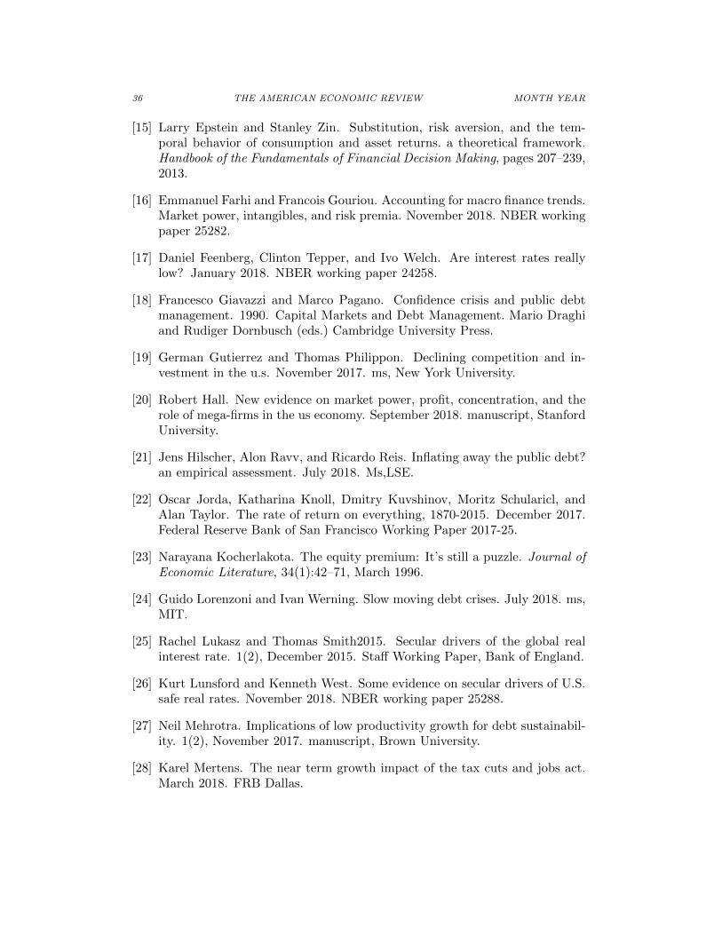
36 THE AMERICAN ECONOMIC REVIEW MONTH YEAR
[15] Larry Epstein and Stanley Zin. Substitution, risk aversion, and the tem-poral behavior of consumption and asset returns. a theoretical framework.Handbook of the Fundamentals of Financial Decision Making, pages 207–239,2013.
[16] Emmanuel Farhi and Francois Gouriou. Accounting for macro finance trends.Market power, intangibles, and risk premia. November 2018. NBER workingpaper 25282.
[17] Daniel Feenberg, Clinton Tepper, and Ivo Welch. Are interest rates reallylow? January 2018. NBER working paper 24258.
[18] Francesco Giavazzi and Marco Pagano. Confidence crisis and public debtmanagement. 1990. Capital Markets and Debt Management. Mario Draghiand Rudiger Dornbusch (eds.) Cambridge University Press.
[19] German Gutierrez and Thomas Philippon. Declining competition and in-vestment in the u.s. November 2017. ms, New York University.
[20] Robert Hall. New evidence on market power, profit, concentration, and therole of mega-firms in the us economy. September 2018. manuscript, StanfordUniversity.
[21] Jens Hilscher, Alon Ravv, and Ricardo Reis. Inflating away the public debt?an empirical assessment. July 2018. Ms,LSE.
[22] Oscar Jorda, Katharina Knoll, Dmitry Kuvshinov, Moritz Schularicl, andAlan Taylor. The rate of return on everything, 1870-2015. December 2017.Federal Reserve Bank of San Francisco Working Paper 2017-25.
[23] Narayana Kocherlakota. The equity premium: It’s still a puzzle. Journal ofEconomic Literature, 34(1):42–71, March 1996.
[24] Guido Lorenzoni and Ivan Werning. Slow moving debt crises. July 2018. ms,MIT.
[25] Rachel Lukasz and Thomas Smith2015. Secular drivers of the global realinterest rate. 1(2), December 2015. Staff Working Paper, Bank of England.
[26] Kurt Lunsford and Kenneth West. Some evidence on secular drivers of U.S.safe real rates. November 2018. NBER working paper 25288.
[27] Neil Mehrotra. Implications of low productivity growth for debt sustainabil-ity. 1(2), November 2017. manuscript, Brown University.
[28] Karel Mertens. The near term growth impact of the tax cuts and jobs act.March 2018. FRB Dallas.

VOL. VOLUME NO. ISSUE DEBT AND RATES 37
[29] Wataru Miyamoto, Thuy Lan Nguyen, and Dmitry Sergeyev. Governmentspending multipliers under the zero lower bound: Evidence from Japan.American Economic Journal: Macroeconomics, 10(3):247–277, 2018.
[30] Thomas Philippon. A primer on concentration, investment, and growth.August 2017. Prepared for the Jackson Hole Economic Policy Symposium.
[31] Lukasz Rachel and Lawrence Summers. The equilibrium real interest rate inadvanced economies: The role of of government policies and current accountimbalances. July 2018. ms, Harvard and LSE.
[32] Valerie Ramey. Can government purchases stimulate the economy? Journalof Economic Literature, 49(3):673–685, September 2011.
[33] Valerie Ramey and Sarah Zubairy. Government spending multipliers in goodtimes and in bad: Evidence from u.s. historical data. 2018. ms, forthcoming,JPE.
[34] Paul Schelzing. Eight centuries of global real rates and the supraseculardecline, 1311-2018. November 2018. ms, Harvard University.
[35] Louise Sheiner. The effects of low productivity growth on fiscal sustainability.May 2018. ms, Peterson Institute for International Economics.
[36] Robert Shiller. Market Volatility. MIT Press, 1992.
[37] Lawrence Summers. What is the social return to capital investment? pages113–141, 1990. in “Growth, Productivity, and Unemployment, Essays inhonor of Robert Solow”, Peter Diamond editor, MIT Press.
[38] Lawrence Summers. Demand side secular stagnation. American EconomicReview Papers and Proceedings, 105:60–65, May 2001.
[39] Philippe Weil. Nonexpected utility in macroeconomics. Quarterly Journalof Economics, 105(1):29–42, February 1990.
[40] Philippe Weil. Overlapping generations: The first Jubilee. Journal of Eco-nomic Perspectives, 22(4):115–134, 2008.
[41] Itzhak Zilcha. Characterizing efficiency in stochastic overlapping generationsmodels. Journal of Economic Theory, 55:1–16, 1991.