PTools tutorial - Institut de Biologie Physico-Chimique ... · PTools tutorial Adrien Saladin 1;2 S ... From the download section 2, ... In the Tests directory, one can test that

PTools tutorial

Adrien Saladin 1,2 Sebastien Fiorucci1,4 Pierre Poulain3

Chantal Prevost2 and Martin Zacharias1

January 16, 2009

1 Computational Biology, School of Engineering and Science, Jacobs University Bremen, 28759 Bremen, Germany

2 LBT, CNRS UPR 9080 and Univ. Paris Diderot - Paris 7, IBPC, 13 rue Pierre et Marie Curie, 75005 Paris, France

3 DSIMB team, Inserm UMR-S 665 and Univ. Paris Diderot - Paris 7, INTS, 6 rue Alexandre Cabanel, 75015 Paris, France

4 LCMBA, UMR-CNRS 6001, Faculte des Sciences, Universite de Nice-Sophia Antipolis, 06108 Nice Cedex 2, France.

This tutorial presents the PTools library features and its docking application ATTRACT.

Contents

1 Set up, compilation and installation 31.1 Basic requirements . . . . . . . . . . . . . . . . . . . . . . . . . . . . . . . . 31.2 Installing prerequisites . . . . . . . . . . . . . . . . . . . . . . . . . . . . . . 3

1.2.1 On Debian or Debian-like systems (Ubuntu) . . . . . . . . . . . . . . 31.2.2 On Fedora systems . . . . . . . . . . . . . . . . . . . . . . . . . . . . 31.2.3 gccxml . . . . . . . . . . . . . . . . . . . . . . . . . . . . . . . . . . . 41.2.4 Pyplusplus and Pygccxml: . . . . . . . . . . . . . . . . . . . . . . . 4

1.3 Compilation . . . . . . . . . . . . . . . . . . . . . . . . . . . . . . . . . . . . 51.3.1 Static pure C++ library . . . . . . . . . . . . . . . . . . . . . . . . . 51.3.2 The library as a Python module . . . . . . . . . . . . . . . . . . . . . 5

1.4 Final test and further documentation . . . . . . . . . . . . . . . . . . . . . . 51.4.1 C++ library only . . . . . . . . . . . . . . . . . . . . . . . . . . . . . 51.4.2 Python module . . . . . . . . . . . . . . . . . . . . . . . . . . . . . . 6

2 PTools library usages and capabilities 62.1 Directly from C++ . . . . . . . . . . . . . . . . . . . . . . . . . . . . . . . . 62.2 From Python through the C++ binding . . . . . . . . . . . . . . . . . . . . 6

2.2.1 Rigidbody objects . . . . . . . . . . . . . . . . . . . . . . . . . . . . . 62.2.2 Selection objects . . . . . . . . . . . . . . . . . . . . . . . . . . . . . 82.2.3 atom objects . . . . . . . . . . . . . . . . . . . . . . . . . . . . . . . 8

3 Docking with PTools: ATTRACT 93.1 Protein–protein complex: 1CGI . . . . . . . . . . . . . . . . . . . . . . . . . 9

3.1.1 Extraction of the docking partners . . . . . . . . . . . . . . . . . . . 93.1.2 Coarse grain reduction . . . . . . . . . . . . . . . . . . . . . . . . . . 103.1.3 Initial ligand positions . . . . . . . . . . . . . . . . . . . . . . . . . . 113.1.4 ATTRACT parameters . . . . . . . . . . . . . . . . . . . . . . . . . . 123.1.5 Simple optimization . . . . . . . . . . . . . . . . . . . . . . . . . . . 123.1.6 Systematic docking simulation . . . . . . . . . . . . . . . . . . . . . . 153.1.7 Docking output analysis . . . . . . . . . . . . . . . . . . . . . . . . . 15

3.2 Protein–DNA complex: 1K79 . . . . . . . . . . . . . . . . . . . . . . . . . . 173.2.1 Extraction of the docking partners . . . . . . . . . . . . . . . . . . . 183.2.2 Coarse grain reduction . . . . . . . . . . . . . . . . . . . . . . . . . . 183.2.3 Initial ligand position . . . . . . . . . . . . . . . . . . . . . . . . . . . 193.2.4 ATTRACT parameters . . . . . . . . . . . . . . . . . . . . . . . . . . 193.2.5 Simple optimization . . . . . . . . . . . . . . . . . . . . . . . . . . . 203.2.6 Systematic docking simulation . . . . . . . . . . . . . . . . . . . . . . 203.2.7 Docking output analysis . . . . . . . . . . . . . . . . . . . . . . . . . 20

3.3 Accurate bead representation . . . . . . . . . . . . . . . . . . . . . . . . . . 21

4 Misc. tips and tricks 224.1 Troubleshooting . . . . . . . . . . . . . . . . . . . . . . . . . . . . . . . . . . 22

4.1.1 Bus error . . . . . . . . . . . . . . . . . . . . . . . . . . . . . . . . . 22

2

1 Set up, compilation and installation

1.1 Basic requirements

The basic requirements are:

• g++ (4.x)

• gfortran (4.x) or g77

• doxygen (optional)

• the Boost C++ library

• SCons

The following tools are also necessary in order to use the library as a Python module:

• Python 2.4 or 2.5 and its development library (python2.4-dev or python2.5-dev)

• gccxml (may require cmake and cvs if you need to compile it from sources).

• pygccxml

• py++

• the Boost.Python library (which is not part of the main Boost C++ library on somelinux distributions)

Software locations and install instructions will be given below.In the following, we assume the PTools library will be installed in the $HOME/soft directorywhere $HOME represents the home directory (usually /home/adrien for the user adrien).

1.2 Installing prerequisites

1.2.1 On Debian or Debian-like systems (Ubuntu)

apt-get install scons libboost-dev libbost-python-dev gccxml

See 1.2.4 for installing necessary tools for building python bindings.Note: some Debian Ubuntu systems have an old version of gccxml that doesn’t work well forbinding this library. If bindings generation or unit tests fail, you should consider installinggccxml manually (see 1.2.3)gccxml versions ≤ 0.6 crash during bindings generation. gccxml v. 0.9 from Debian Lennycontains a bug that prevents all Python unit tests to work (test 16 fails).

1.2.2 On Fedora systems

SCons (make substitute): The scons package provided by Fedora is not up-to-dateenough to link Fortran and C++ together and then rise an error. The last version of sconsis obtained at the homepage of the project (http://www.scons.org/). From the downloadsection 1, get the stable file scons-0.98.5-1.noarch.rpm and install it:

rpm -ivh scons-0.98.5-1.noarch.rpm

1http://sourceforge.net/project/showfiles.php?group_id=30337

3

Note: SCons 0.98.5 and 1.0.0 were successfully testedYou can then install some packages:

yum install boost boost-devel python-devel

After that, you still need to manually install gccxml, pyplusplus and pygccxml (see below).

1.2.3 gccxml

The homepage of gccxml project is http://www.gccxml.org and its official CVS repositoryis http://www.gccxml.org/HTML/Download.html.

cvs -d :pserver:[email protected]:/cvsroot/GCC_XML login

(just press enter when prompted for a password)Follow this command by checking out the source code:

cvs -d :pserver:[email protected]:/cvsroot/GCC_XML co gccxml

mkdir gccxml-build

cd gccxml-build

cmake ../gccxml -DCMAKE_INSTALL_PREFIX:PATH=/installation/path

make

make install

The -DC_MAKE_INSTALL_PREFIX option can be left off if you want to use /usr/local as theinstallation prefix.

1.2.4 Pyplusplus and Pygccxml:

The homepage of pyplusplus and pygccxml projects is http://www.language-binding.net/pyplusplus/pyplusplus.html.From the download section 2, get the files pygccxml-0.9.5.zip and Py++-0.9.5.zip.

unzip pygccxml-0.9.5.zip

cd pygccxml-0.9.5/

python setup.py build

python setup.py install --prefix=$HOME/soft

unzip Py++-0.9.5.zip

cd Py++-0.9.5/

python setup.py build

python setup.py install --prefix=$HOME/soft

In your $HOME/.bashrc file, then add:

export PATH=PATH:$HOME/soft/bin/

export PYTHONPATH=$HOME/soft/lib/python2.4/site-packages/

In a Python shell (obtained with the python command), test the installation of PyPlusPlus:

>>> import pyplusplus

2https://sourceforge.net/project/showfiles.php?group_id=118209

4

1.3 Compilation

Dowload the PTools library and untar it:

tar zxvf ptools-XX.tar.gz

The directory ptools-XX should be created.

1.3.1 Static pure C++ library

Move into the new directory and type:

scons cpp

This should create the file libptools.a.If SCons cannot locate a fortran compiler or a library, you can define a search path at thebeginning of the SConstruct file.

1.3.2 The library as a Python module

From the PTools main directory ($HOME/soft/ptools-XX), first create the Python/C++interface:

python interface.py

Then compile the library:

scons

Note that scons -j2 compiles with two processors in parallel.If SCons cannot locate a fortran compiler or a library, you can define a search path at thebeginning of the SConstruct file.

1.4 Final test and further documentation

1.4.1 C++ library only

The PTools library has a new C++ unit test system. To try it move into the Tests/ directoryand type:

make testcpp

You should get something like this:

running C++ tests

python cxxtestgen.py --error-printer ptoolstest.h > runner.cpp

g++ runner.cpp -I.. -I. -L.. -lptools -o ptoolstest.bin

./ptoolstest.bin

Running 15 tests...............OK!

5

1.4.2 Python module

In the Tests directory, one can test that the compilation worked:

python unittest1.py

The expected output should be similar to:

...............

----------------------------------------------------------------------

Ran 16 tests in 0.316s

OK

2 PTools library usages and capabilities

2.1 Directly from C++

Source code may be parsed by Doxygen, an automatic documentation generator. This doc-umentation may help for the C++ (and indirectly for the Python) part of the library.If Doxygen is installed, simply type doxygen in the directory which contains the Doxyfile

($HOME/soft/ptools-XX). Then look into the html directory and open with your favoriteweb browser the index.html file generated by doxygen.The most important objects and functions to manipulate PDB files are explained in thefollowing section.

2.2 From Python through the C++ binding

If PTools has been installed in the $HOME/soft/ptools-XX directory, update your PYTHONPATHenvironment variable accordingly:

export PYTHONPATH=$PYTHONPATH:$HOME/soft/ptools-XX/

or add this line at the end of your $HOME/.bashrc file.From the Python interpreter or from a Python script, first load the PTools library:

from ptools import *

2.2.1 Rigidbody objects

Load PDB file (for instance 1BTA.pdb) into a rigidbody object.

pdb = Rigidbody("1BTA.pdb")

Number of atoms.

pdb.Size()

Maximum distance (in A) from geometric center.

pdb.Radius()

Radius of gyration (in A).

pdb.RadiusGyration()

6

Structure translation. First create a translation vector as a Coord3D object (for instance+5 A along the X axis, -3 A along Y and +1 A along the Z axis):

trans = Coord3D(5, -3, 1)

Then, apply the translation vector trans:

pdb.Translate(trans)

Center structure to origin.

pdb.CenterToOrigin()

Save structure as PDB file.

WritePDB(pdb, "1BTA_centered.pdb")

Superpose two structures. This is a complete example where we superpose a structureand its copy after a translation.

First, load a PDB file as a Rigidbody object

pdb = Rigidbody("1BTA.pdb")

Make a copy

pdb2 = Rigidbody(pdb)

Create a translation vector

trans = Coord3D(5, 0, 1)

Apply the translation on the copy

pdb2.Translate(trans)

Superpose both structures

sup = superpose(pdb, pdb2)

Extract RMSD and matrix

rmsd = sup.rmsd

matrix = sup.matrix

Print RMSD

print rmsd

The output is 1.22224104574e-07 (in A). Then print the 4× 4 matrix:

matrix.Print()

with output:

1 8.07909e-09 -5.80388e-09 1.42535e-09

-8.07909e-09 1 2.0426e-09 2.54026e-08

5.80388e-09 -2.0426e-09 1 -1.86091e-08

0 0 0 1

7

2.2.2 Selection objects

Select CA atoms.

sel_ca = pdb.CA()

Select backbone atoms.

sel_bkbn = pdb.Backbone()

Select by chain.

sel_chainA = pdb.SelectChainId("A")

sel_chainB = pdb.SelectChainId("B")

Select a range of residues.

sel_res = pdb.SelectResRange(10, 20)

Get the number of atomes (the size) of a selection.

sel_res.Size()

Reunion between two selections.

sel_chainAB = sel_chainA | sel_chainB

or directly

sel_chainAB = pdb.SelectChainId("A") | pdb.SelectChainId("B")

Convert selection to rigidbody object.

ca_trace = sel_ca.CreateRigid()

2.2.3 atom objects

Copy atom from rigidbody object. In this example, the third atom (indexed as 2 sincethe first atom in numberered 0) is copied.

at = pdb.CopyAtom(2)

Set new coordinates

new_XYZ = Coord3D(2.1,3.9,5.5)

at.SetCoords(new_XYZ)

Translate atom

vector = Coord3D(1.0,1.0,1.0)

at.Translate(vector)

Print atom in pdb-like format

at.ToPdbString()

8

Get atom properties

at.GetType()

at.GetResidType()

at.GetAtomCharge()

at.GetChainId()

at.GetResidId()

at.GetAtomId()

at.GetExtra()

Set atom properties

at.SetType()

at.SetResidType()

at.SetAtomCharge()

at.SetChainId()

at.SetResidId()

at.SetAtomId()

at.SetExtra()

3 Docking with PTools: ATTRACT

This part shows the PTools docking application called ATTRACT[3]. It usage and capabili-ties are illustrated by the docking of a protein–protein complex (1CGI) and a protein–DNAcomplex[1] (1K79). The first example (1CGI) is explained step by step and scripts usagesare exhaustively detailled. The second example (1K79) is much more straightforward.

3.1 Protein–protein complex: 1CGI

The 1CGI complex 3 has two partners,

• the bovine chymotrypsinogen A: chain E, 245 residues, 1799 atoms

• a variant of the human pancreatic secretory trypsin inhibitor: chain I, 56 residues, 440atoms

3.1.1 Extraction of the docking partners

Before docking, one has to separate both partners. This is possible with vizualisation softwaresuch as Pymol 4 or VMD 5, and also directly with PTools.Within the Python interpreter, first load the PTools library:


Read the PDB file of the complex:

pdb=Rigidbody("1CGI.pdb")

The chain selection allows the separation between chain E and I.

3http://www.rcsb.org/pdb/cgi/explore.cgi?pdbId=1CGI4http://pymol.sourceforge.net/5http://www.ks.uiuc.edu/Research/vmd/

9

selectE=pdb.SelectChainId("E")

selectI=pdb.SelectChainId("I")

Create both chains as independant Rigidbody objects and save them in PDB files. Thelargest protein is defined as the receptor (chain E) and the smallest as the ligand (chain I).

protE=selectE.CreateRigid()

protI=selectI.CreateRigid()

WritePDB(protE,"receptor.pdb")

WritePDB(protI,"ligand.pdb")

Or more quickly:

WritePDB(selectE.CreateRigid(),"receptor.pdb")

WritePDB(selectI.CreateRigid(),"ligand.pdb")

3.1.2 Coarse grain reduction

This step translates all-atom molecules into coarse grain (reduced) molecules for furtherdocking.For the receptor:

./reduce.py --prot receptor.pdb > receptor.red

In the present case, receptor.red contains 522 beads.

For the ligand:

./reduce.py --prot ligand.pdb > ligand.red

In this example, ligand.red contains 126 beads.

The reduce.py script requires the following parameters:

• --prot or --dna option, specifies the type of molecule to reduce (respectively proteinor DNA)

• an input all-atom PDB file, for instance receptor.pdb

• an output coarse grain file, for instance receptor.red

This script also needs some definition files:

• beads topology files (at2cg.prot.dat for protein reduction and at2cg.dna.dat forDNA reduction )

• forcefield parameters file (ff_param.dat)

• filetypes conversion file (type_conversion.dat)

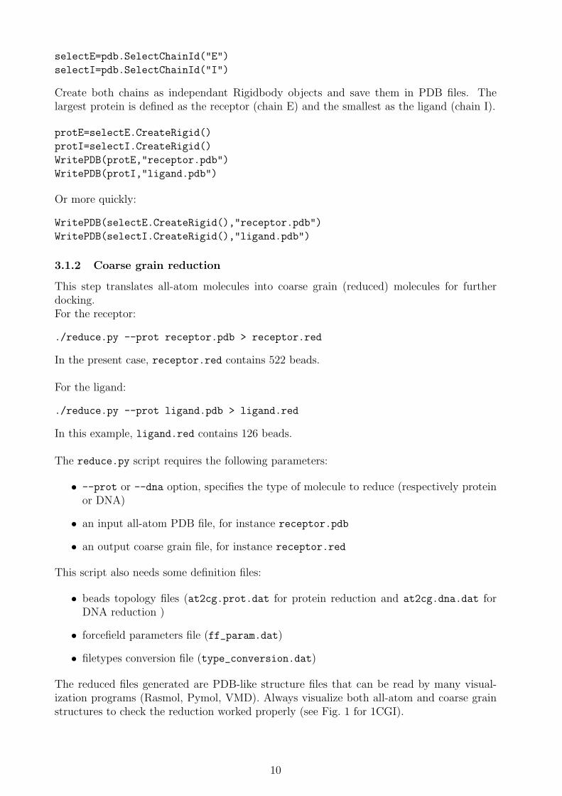
The reduced files generated are PDB-like structure files that can be read by many visual-ization programs (Rasmol, Pymol, VMD). Always visualize both all-atom and coarse grainstructures to check the reduction worked properly (see Fig. 1 for 1CGI).

10

A B

Figure 1: All-atom (green sticks) and reduced (red spheres) representation of both proteinsin the 1CGI complex. Receptor (A) and ligand (B).

3.1.3 Initial ligand positions

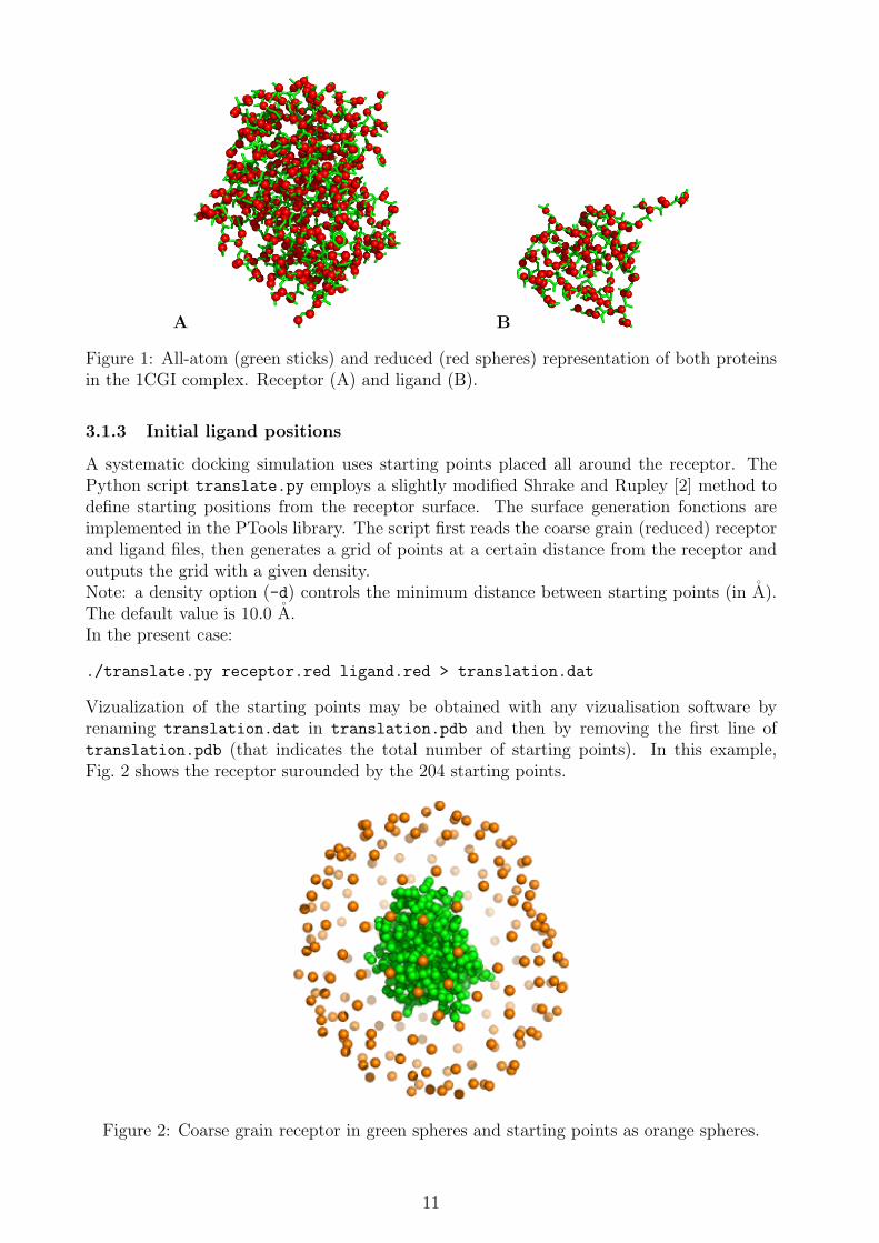
A systematic docking simulation uses starting points placed all around the receptor. ThePython script translate.py employs a slightly modified Shrake and Rupley [2] method todefine starting positions from the receptor surface. The surface generation fonctions areimplemented in the PTools library. The script first reads the coarse grain (reduced) receptorand ligand files, then generates a grid of points at a certain distance from the receptor andoutputs the grid with a given density.Note: a density option (-d) controls the minimum distance between starting points (in A).The default value is 10.0 A.In the present case:

./translate.py receptor.red ligand.red > translation.dat

Vizualization of the starting points may be obtained with any vizualisation software byrenaming translation.dat in translation.pdb and then by removing the first line oftranslation.pdb (that indicates the total number of starting points). In this example,Fig. 2 shows the receptor surounded by the 204 starting points.

Figure 2: Coarse grain receptor in green spheres and starting points as orange spheres.

11

For each position in translation (each ATOM line of the file translation.dat), there are 258associated rotations defined in the file rotation.dat.

3.1.4 ATTRACT parameters

ATTRACT parameters are found in the file attract.inp, which typical content is :

6 0 01

-34.32940 38.75490 -3.66956 0.000502

100 2 1 1 1 0 0 0 1 9900.003

100 2 1 1 1 0 0 0 1 1500.004

100 2 1 1 1 0 0 0 1 1000.005

50 2 1 1 1 0 0 0 0 500.006

50 2 1 1 1 0 0 0 0 500.007

50 2 1 1 1 0 0 0 0 500.008

Line 1 indicates the number of minimisations performed by ATTRACT for each startingposition (six in the present case). The last six lines (3–8) are the characteristics of eachminimisation. The first column is the number of steps before the minimisation stops. Thelast column is the square of the cutoff distance for the calculation of the interaction energybetween both partners. In the present case, the simulation starts with a very large cutoffvalue of 9900 A2 (∼ 99 A), which is gradually dicreased to end with 500 A2 (∼ 22 A).

Note: Columns with zeros or ones should not be modified, as well as line 2. They are usedfor internal development purposes.

3.1.5 Simple optimization

A standard simulation with ATTRACT requires:

• the ATTRACT Python script (Attract.py)

• a coarse grain receptor (fixed partner) file (receptor.red)

• a coarse grain (mobile partner) file (ligand.red)

• the coarse grain parameters (aminon.par)

• translation starting points (translation.dat)

• rotations performed for each translation starting point (rotation.dat)

• docking parameters (attract.inp)

ATTRACT can be used with different options:

• -s, performs one single serie of minimisations with the ligand in its initial position.

• --ref, (optional) provides a ligand PDB file as a reference (reduced). After eachdocking, the RMSD is calculated between this reference structure and the simulatedligand.

• --t transnb, loads only the translation number transnb (and all its associated ro-tations). This option is very usefull for dispatching a simulation over a cluster ofcomputers.

12

A single ATTRACT simulation (optimization) may thus be obtained by:

./Attract.py receptor.red ligand.red --ref=ligand.red -s > single.att

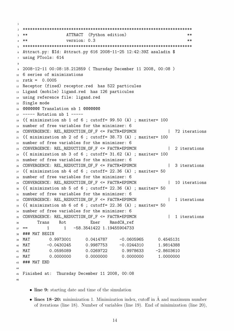
The first PDB file provided must be the receptor file (and the second the ligand). Thecontent of the output file single.att is the following:

13

1

**********************************************************************2

** ATTRACT (Python edition) **3

** version: 0.3 **4

**********************************************************************5

Attract.py: $Id: Attract.py 616 2008-11-25 12:42:39Z asaladin $6

using PTools: 6147

8

2008-12-11 00:08:18.212859 ( Thursday December 11 2008, 00:08 )9

6 series of minimizations10

rstk = 0.000511

Receptor (fixed) receptor.red has 522 particules12

Ligand (mobile) ligand.red has 126 particules13

using reference file: ligand.red14

Single mode15

@@@@@@@ Translation nb 1 @@@@@@@16

----- Rotation nb 1 -----17

{{ minimization nb 1 of 6 ; cutoff= 99.50 (A) ; maxiter= 10018

number of free variables for the minimizer: 619

CONVERGENCE: REL_REDUCTION_OF_F <= FACTR*EPSMCH | 72 iterations20
















Trans Rot Ener RmsdCA_ref36

== 1 1 -58.3541422 1.1945590473337

### MAT BEGIN38

MAT 0.9973001 0.0414787 -0.0605965 0.454513139

MAT -0.0430245 0.9987753 -0.0244310 1.981438840

MAT 0.0595089 0.0269722 0.9978633 -2.860361041

MAT 0.0000000 0.0000000 0.0000000 1.000000042

### MAT END43

44

Finished at: Thursday December 11 2008, 00:0845

46

• line 9: starting date and time of the simulation

• lines 18–20: minimization 1. Minimization index, cutoff in A and maximum numberof iterations (line 18). Number of variables (line 19). End of minimization (line 20),

14

either convergence is achieved (the number of performed iterations is specified), eithermaximum number of steps is reached.

• lines 21–23: minimization 2.





• lines 36–37: final result after the 6 minimizations. With a single series of minimiza-tion, the default translation (Trans) is 1 and the default rotation (Rot) is 1. Energy(Ener) is given in RT unit and the Cα-RMSD (RmsdCA_ref) in A if the --ref optionis specified.

• lines 38–43: rotation/translation matrix of the ligand compared to its initial position.

• line 45: end date and time of the simulation.

Here, the final energy is -58.4 RT unit and the RMSD is 1.2 A, which is pretty close fromthe initial position. (In a perfect simulation, RMSD would be, of course, 0.0 A).

3.1.6 Systematic docking simulation

For a full systematic docking in the translational and rotational space (using both translation.dat

and rotation.dat files), the command line is:

./Attract.py receptor.red ligand.red --ref=ligand.red > docking.att &

The output file docking.att contains all informations on the docking simulation. It containsthe ouput of all series of minimizations (with the specification of translation and rotationnumber).For the 1CGI complex, the systematic docking took 19 hours on a single processor of a64 bit Intel Xeon 1.86 GHz 2 Go RAM computer. The size of the output file docking.att

is roughly 77 Mo.

3.1.7 Docking output analysis

The 10 best geometries found during the docking simulation can be listed with

cat docking.att | egrep -e "^==" | sort -n -k4 | head

For the previsous docking simulation of 1CGI, this gives:

== 133 92 -58.3541443 1.19429783478

== 73 229 -58.3541441 1.19413397471

== 133 21 -58.3541437 1.19566121232

== 73 235 -58.3541436 1.19394986862

== 136 21 -58.3541424 1.19584401069

== 130 141 -58.3541411 1.1930478392

== 194 219 -58.3541410 1.1961246513

== 73 7 -58.3541406 1.19314844151

== 136 155 -58.3541400 1.19273140092

== 163 70 -58.3541387 1.19596166869

15

With each column meaning:

1. tag characters (==) to quickly find the result of each set of minimizations

2. translation number (starts at 1)

3. rotation number (starts at 1)

4. final energy of the complex in RT unit

5. final RMSD in A, if the --ref option is provided.

Any simulated ligand structure can be extracted with the script Extract.py:

./Extract.py docking.att ligand.red 133 92 > ligand_1.red

with the parameters:

• the ouput file of the docking simulation (docking.att)

• the initial ligand file (ligand.red)

• a translation number (133)

• a rotation number (92)

• an output ligand file (ligand_1.red)

Fig. 3 shows the best solution of the docking simulation and the reference complex. With aRMSD of 1.2 A between both structures, the docking simulation found very well the initialcomplex structure.

A B

Figure 3: Reduced representations of receptor (green), ligand at reference position (red) andligand from the best solution (lowest energy) of the docking (blue). Front (A) and top (B)views. Beads have exact van der Waals radii.

In case an experimental structure of the system is known (as in this example), it is possibleto calculate the interface RMSD (iRMSD) and the native fraction (fnat) as defined by theCAPRI contest 6 using the following scripts:

irmsd.py receptor.red ligand.red ligand_1.red

fnat.py receptor.red ligand.red ligand_1.red

For iRMSD, output is in A and fnat is given as a proportion (between 0.0 and 1.0). Param-eters are defined as:

6http://capri.ebi.ac.uk

16

• the receptor file (receptor.red)


• the output ligand file (ligand_1.red)

Our clustering algorithm implemented in cluster.py can rapidly filter near identical solu-tions without requiring a preselected number of desired clusters. The algorithm is based onRMSD comparison and an additional energy criterion can be included (see script options,by default RMSD and energy criterions are 1 A and 1 RT unit respectively).

cluster.py docking.att ligand.red > docking.clust

with the parameters:

• an ouput of the docking simulation (docking.att)


• an output cluster file (docking.clust)

The first lines of the output cluster file are:

Trans Rot Ener RmsdCA_ref Rank Weight1

== 133 92 -58.3541443 1.1942978 1 552

== 196 132 -40.3704483 48.8195971 2 13

== 164 212 -39.3828793 6.4968451 3 24

== 71 102 -38.7843145 14.7084754 4 145

== 73 126 -38.5826662 11.5175880 5 36

== 129 223 -38.3872389 12.3477797 6 37

== 132 245 -38.3429828 14.0028863 7 108

== 133 131 -38.1570360 16.0382603 8 179

Line 1 is a comment line, next lines are clusters. For each cluster (line) is specified:

• a representative structure with the corresponding translation and rotation numbers(column 2, Trans, and 3, Rot), interaction energy (column 4, Ener) and RMSD (column5, RmsdCA_ref) from the reference ligand structure

• the number of the cluster (column 6, Rank)

• the number of structures (docking solutions) in this cluster (column 7, Weight)

The large weight of the best solution shows the very good convergence of the docking simu-lation.

3.2 Protein–DNA complex: 1K79

The 1K79 complex 7 has two partners,

• the ETS protein: chain A, 104 residues, 873 atoms (defined in the following as thereceptor)

• a DNA molecule: chain B and C, 30 bases, 607 atoms (defined in the following as theligand)

7http://www.rcsb.org/pdb/cgi/explore.cgi?pdbId=1K79

17

3.2.1 Extraction of the docking partners

Both partners are extracted automatically with PTools from the Python interpreter:


pdb=Rigidbody("1K79.pdb")

selA=pdb.SelectChainId("A")

selB=pdb.SelectChainId("B")

selC=pdb.SelectChainId("C")

WritePDB(selA.CreateRigid(), "receptor.pdb")

WritePDB( (selB | selC).CreateRigid(), "ligand.pdb")

exit()

3.2.2 Coarse grain reduction

All-atom molecules are then translated into coarse grain (reduced) molecule for further dock-ing.For the receptor (protein):

./reduce.py --prot receptor.pdb --warnonly > receptor.red

This command generates few warnings due to missing atoms in the Lys436 residue. Whenan atom is missing, the corresponding bead is not created. You will have to check if this isan important issue for your system and fix your PDB with your favourite tool. Please alsonote that the reduce script doesn’t report anything you if a complete residue is missing (thisfrequently occurs in loops).

./reduce.py --prot receptor.pdb > receptor.red

./at2cg.prot.dat: found the definition of residues ARG GLU GLN LYS TRP MET PHE TYR HIS GLY ASN ALA ASP CYS ILE LEU PRO SER THR VAL

./at2cg.prot.dat: created the partition for residues ARG(3 beads) GLU(3 beads) GLN(3 beads) LYS(3 beads) TRP(3 beads) MET(3 beads) PHE(3 beads) TYR(3 beads) HIS(3 beads) GLY(1 beads) ASN(2 beads) ALA(2 beads) ASP(2 beads) CYS(2 beads) ILE(2 beads) LEU(2 beads) PRO(2 beads) SER(2 beads) THR(2 beads) VAL(2 beads)

./ff_param.dat: reading force field parameters for bead 1 2 3 4 5 6 7 8 9 10 11 12 13 14 15 16 17 18 19 20 21 22 23 24 25 26 27 28 29 30 31 32 33 34 35 36 37 38 39 40 41 42

Load atomic file receptor.pdb with 873 atoms

Number of residues: 104

Reading all atoms and filling beads:

Coarse graining:

ERROR: missing atom CG in bead CB 16 for residue LYS 436. Please fix your PDB!

Continue execution as required ...

ERROR: missing atom CE in bead CE 17 for residue LYS 436. Please fix your PDB!


Coarse grain (reduced) output: 246 beads

The reduced protein, receptor.red, contains 246 beads.

For the ligand (DNA), do not forget the --dna option:

./reduce.py --dna ligand.pdb --warnonly > ligand.red

This also generates few warnings due to incomplete bases:

./at2cg.dna.dat: found the definition of residues A G C T

./at2cg.dna.dat: created the partition for residues A(6 beads) G(6 beads) C(5 beads) T(5 beads)

./ff_param.dat: reading force field parameters for bead 1 2 3 4 5 6 7 8 9 10 11 12 13 14 15 16 17 18 19 20 21 22 23 24 25 26 27 28 29 30 31 32 33 34 35 36 37 38 39 40 41 42

Load atomic file ligand.pdb with 607 atoms

Number of residues: 30

18

Reading all atoms and filling beads:

Coarse graining:

ERROR: missing atom O1P in bead GP1 30 for residue T 1. Please fix your PDB!


ERROR: missing atom O2P in bead GP1 30 for residue T 1. Please fix your PDB!


ERROR: missing atom P in bead GP1 30 for residue T 1. Please fix your PDB!


ERROR: missing atom O1P in bead GP1 30 for residue C 1. Please fix your PDB!


ERROR: missing atom O2P in bead GP1 30 for residue C 1. Please fix your PDB!


ERROR: missing atom P in bead GP1 30 for residue C 1. Please fix your PDB!


Coarse grain (reduced) output: 162 beads

The reduced DNA, ligand.red, ends up with 162 beads.

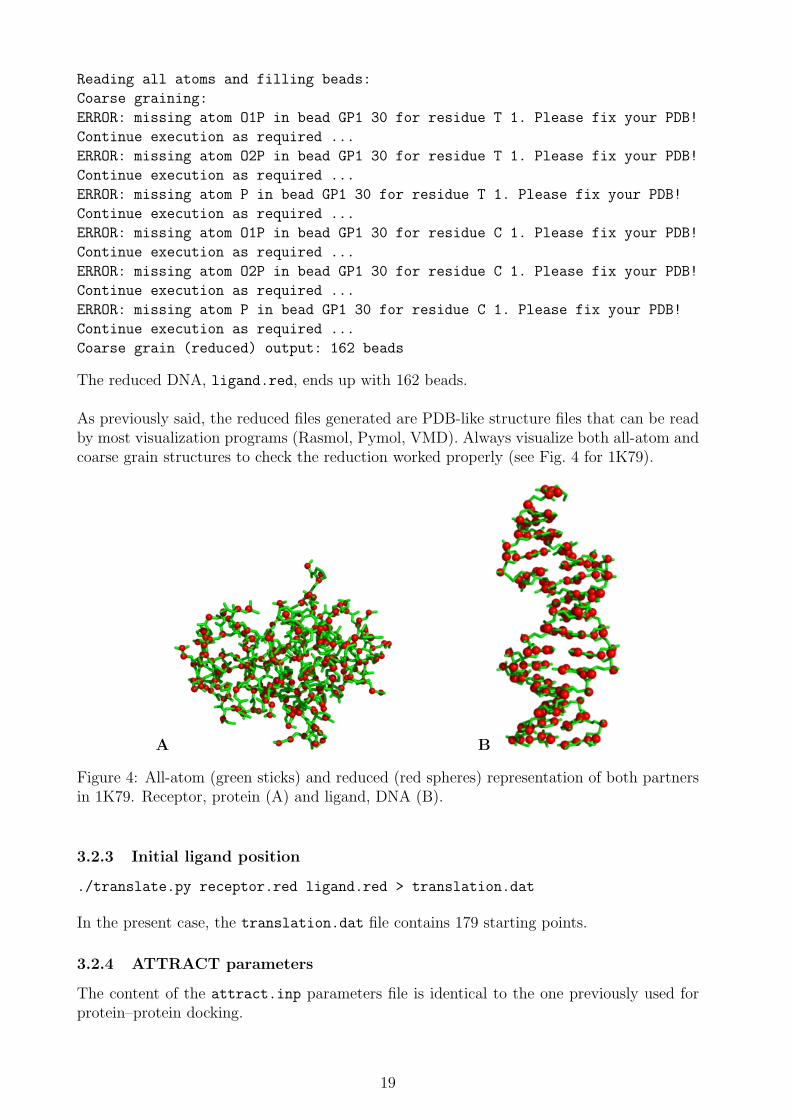
As previously said, the reduced files generated are PDB-like structure files that can be readby most visualization programs (Rasmol, Pymol, VMD). Always visualize both all-atom andcoarse grain structures to check the reduction worked properly (see Fig. 4 for 1K79).

A B

Figure 4: All-atom (green sticks) and reduced (red spheres) representation of both partnersin 1K79. Receptor, protein (A) and ligand, DNA (B).

3.2.3 Initial ligand position

./translate.py receptor.red ligand.red > translation.dat

In the present case, the translation.dat file contains 179 starting points.

3.2.4 ATTRACT parameters

The content of the attract.inp parameters file is identical to the one previously used forprotein–protein docking.

19

3.2.5 Simple optimization

An ATTRACT optimization is done with:

./Attract.py receptor.red ligand.red --ref=ligand.red -s > single.att

Here, the final energy is -38.4 RT unit and the RMSD is 1.3 A which is very close from theinitial position.Please note, that the RMSD is not computed here on Cα atoms since the ligand is a DNAmolecule. The RMSD is calculated with all DNA beads.

3.2.6 Systematic docking simulation

A systematic docking simulation is then:

./Attract.py receptor.red ligand.red --ref=ligand.red > docking.att &

The output file docking.att contains all informations on the docking simulation. It containsthe ouput of all series of minimizations (with the specification of translation and rotationnumbers).For the 1K79 complex, the systematic docking took roughly 11 hours on a single processor ofa 64 bit Intel Xeon 1.86 GHz 2 Go RAM computer. The size of the output file docking.att

is about 67 Mo.

3.2.7 Docking output analysis

The 10 best geometries found during the docking simulation can be listed with :

cat docking.att | egrep -e "^==" | sort -n -k4 | head

This gives:

== 30 157 -38.4463924 1.25369709657

== 169 51 -38.4463903 1.25534808001

== 148 234 -38.4463875 1.25581284912

== 87 257 -38.4463867 1.25409925951

== 109 231 -38.4463855 1.25469537295

== 104 236 -38.4463848 1.25571565339

== 144 27 -38.4463848 1.25495212761

== 164 255 -38.4463819 1.25410121719

== 163 27 -38.4463817 1.25446355377

== 87 241 -38.4463806 1.2554586922

We can then extract the best structure obtained (translation number 30 and rotation number157, illustrated Fig. 5):

./Extract.py docking.att ligand.red 30 157 > ligand_1.red

As for protein–protein example, one can compute the native fraction (fnat).

fnat.py receptor.red ligand.red ligand_1.red

20

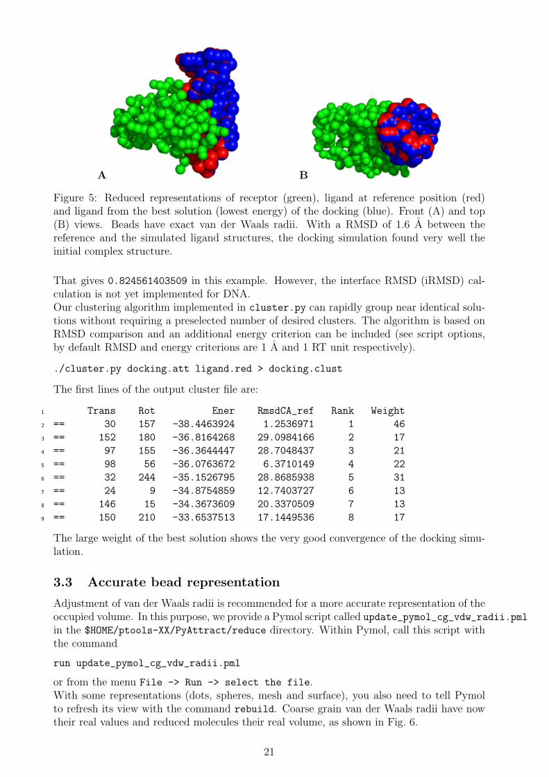
A B

Figure 5: Reduced representations of receptor (green), ligand at reference position (red)and ligand from the best solution (lowest energy) of the docking (blue). Front (A) and top(B) views. Beads have exact van der Waals radii. With a RMSD of 1.6 A between thereference and the simulated ligand structures, the docking simulation found very well theinitial complex structure.

That gives 0.824561403509 in this example. However, the interface RMSD (iRMSD) cal-culation is not yet implemented for DNA.Our clustering algorithm implemented in cluster.py can rapidly group near identical solu-tions without requiring a preselected number of desired clusters. The algorithm is based onRMSD comparison and an additional energy criterion can be included (see script options,by default RMSD and energy criterions are 1 A and 1 RT unit respectively).

./cluster.py docking.att ligand.red > docking.clust

The first lines of the output cluster file are:

Trans Rot Ener RmsdCA_ref Rank Weight1

== 30 157 -38.4463924 1.2536971 1 462

== 152 180 -36.8164268 29.0984166 2 173

== 97 155 -36.3644447 28.7048437 3 214

== 98 56 -36.0763672 6.3710149 4 225

== 32 244 -35.1526795 28.8685938 5 316

== 24 9 -34.8754859 12.7403727 6 137

== 146 15 -34.3673609 20.3370509 7 138

== 150 210 -33.6537513 17.1449536 8 179

The large weight of the best solution shows the very good convergence of the docking simu-lation.

3.3 Accurate bead representation

Adjustment of van der Waals radii is recommended for a more accurate representation of theoccupied volume. In this purpose, we provide a Pymol script called update_pymol_cg_vdw_radii.pml

in the $HOME/ptools-XX/PyAttract/reduce directory. Within Pymol, call this script withthe command

run update_pymol_cg_vdw_radii.pml

or from the menu File -> Run -> select the file.With some representations (dots, spheres, mesh and surface), you also need to tell Pymolto refresh its view with the command rebuild. Coarse grain van der Waals radii have nowtheir real values and reduced molecules their real volume, as shown in Fig. 6.

21

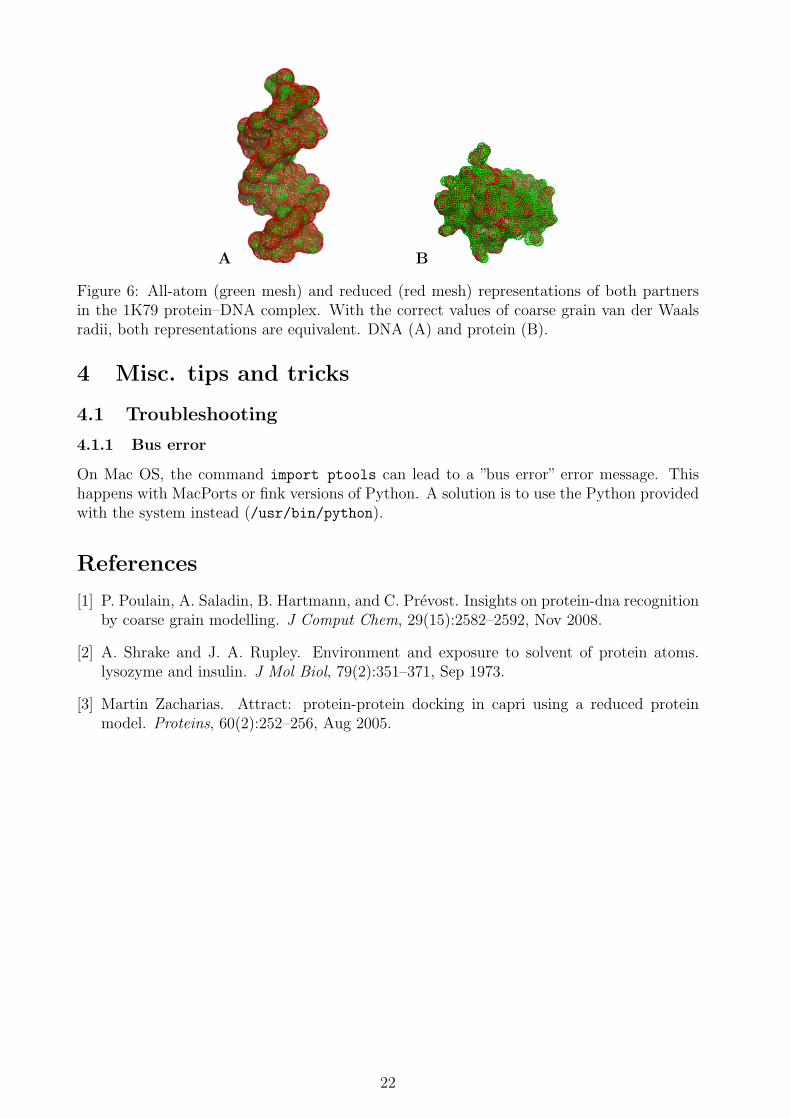
A B

Figure 6: All-atom (green mesh) and reduced (red mesh) representations of both partnersin the 1K79 protein–DNA complex. With the correct values of coarse grain van der Waalsradii, both representations are equivalent. DNA (A) and protein (B).

4 Misc. tips and tricks

4.1 Troubleshooting

4.1.1 Bus error

On Mac OS, the command import ptools can lead to a ”bus error” error message. Thishappens with MacPorts or fink versions of Python. A solution is to use the Python providedwith the system instead (/usr/bin/python).

References

[1] P. Poulain, A. Saladin, B. Hartmann, and C. Prevost. Insights on protein-dna recognitionby coarse grain modelling. J Comput Chem, 29(15):2582–2592, Nov 2008.

[2] A. Shrake and J. A. Rupley. Environment and exposure to solvent of protein atoms.lysozyme and insulin. J Mol Biol, 79(2):351–371, Sep 1973.

[3] Martin Zacharias. Attract: protein-protein docking in capri using a reduced proteinmodel. Proteins, 60(2):252–256, Aug 2005.

22

Documents

PTools tutorial - Institut de Biologie Physico-Chimique ... · PTools tutorial Adrien Saladin 1;2 S ... From the download section 2, ... In the Tests directory, one can test that