PSEUDO-RANDOM NUMBER GENERATOR

by

CLEMENT C.Y. LAM, B.ENG. (McMaster) !

PART B: ON-CAMPUS PROJECT*

A project report submitted in partial fulfillment of the

requirement for the degree of

Master of Engineering

Dept. of Engineering Physics

McMaster University

Hamilton, Ontario

September, 1977

*One of the two project reports: The other part is

designated PART A:McMASTER (Off-Campus) PROJECT.

MASTER OF ENGINEERING (1977)

Department of Engineering Physics

MCMASTER UNIVERSITY

Hamilton, Ontario

TITLE: PSEUDO-RANDOM NUMBER GENERATOR

AUTHOR: Clement C.Y. Lam, B. Eng. (McMaster)

SUPERVISOR: Dr. T.J. Kennett

NUMBER OF PAGES: vi, 45

ii

ABSTRACT

A simple and inexpensive pseudo-random number

generator has been designed and built using linear feed­

back shift registers to generate rectangular and gaussian

distributed numbers. The device has been interfaced to a

Nova computer to provide a high speed source of random

numbers.

The two distributionshave been checked with the

following tests: (i) Frequency test (ii) Autocorrelation

test and (iii) d 2-test. Results of each test have been

compared with the expected theoretical values. Finally,

a comparison of the generating speed has been made between

this new generator and the existing old software generators.

This 28-bit generator is especially desirable in

random simulation and Monte Carlo application if randomness,

speed and cost are the main consideration in the design.

iii

ACKNOWLEDGEMENT

I wish to thank my supervisor, Dr. T.J. Kennett,

for his valuable guidance and suggestions throughout the

course of this project. I also wish to thank Mr. K. Chin

for the helpful discussions I had with him on many

occasions.

iv

LIST OF FIGURES

Figure Page

1.1 General feedback shift register 2

l.2(a) System block diagram(Rectangular distribution) 4

l.2(b) System block diagram(Gaussian distribution) 5

2.1 Interfacing network 9

2.2

2.3

2.4

2.5

2.6

2.7

4.1

4.2

4.3

4.4

4.5

Timing device

28-bit FSR

28-bit FSR(Detailed)

Input

Timing signals when a seed is laid

Timing synchronization in generating a

rectangular number

Frequency curve(Rectangular)

Distribution curve(Rectangular)

Frequency curve of the deviation from the

mean(Rectangular)

Frequency curve(Gaussian)

Distribution curve(Gaussian)

v

10

11

12

13

15

16

27

28

29

30

31

LIST OF TABLES

Table Page

4.1 Autocorrelations of the rectangular 34

distribution

4.2 Autocorrelations of the gaussian 35

distribution

4.3 2 d -test 37

4.4 Speed of existing generators 38

vi

ABSrr·RACT

ACKNOWLEDGEMENT

LIST OF FIGURES

LIST OF TABLES

TABLE OF CONTENTS

CHAPTER 1: INTRODUCTION

1.1 Purpose of the project

1. 2 Theory

1.3 Implementation

CHAPTER 2: HARDWARE DESIGN

2.1 Rectangular distribution

2.2 Gaussian distribution

CHAPTER 3: SOFTWARE CONTROL

3.1 Fortran callable subroutines

3.2 Basic callable subroutines

CHAPTER 4: TESTS AND OBSERVATION

4.1 Frequency test

4.1.1 Rectangular distribution

4.1.2 Gaussian distribution

4.2 Correlation test

4.2.1 Rectangular distribution

Page

iii

iv

v

vi

1

1

1

3

7

7

17

18

18

19

25

25

25

26

32

32

4.2.2 Gaussian distribution

2 4.3 d -test

4.4 Speed consideration

35

36,

38

CHAPTER 5: CONCLUSION 40

APPENDIX A: MAXIMUM-LENGTH SHIFT-REGISTER-SEQUENCE 42

APPENDIX B: I.C. LAYOUT 44

REFERENCES: 45

CHAPTER 1

INTRODUCTION

1.1 Purpose of the project

In a wide variety of simulation and modelling

studies where digital computers are used, a need usually

arises for random number sequences. It is for such app-

lications that most pseudo-random number(PRNG) are de­

signed and built.

1

The PRNG's existing in the laboratory are either too

slow or they are not as random as the user wants them to be.

The need for a new generator which is both fast and has a

longer non-repeating. sequence has led to the design and im­

plementation of the device reported in this project, namely,

a PRNG which could give rectangular distributed or gaussian

distributed numbers.

The objective of the project was to build such a

PRNG using hardware and interface it to the Nova computer.

1.2 Theory(l, 2 , 3 )

The term "random" when applied to numbers or sequences

relates to their origion rather than the numbers or sequences

themselves. (l) By this definition, one could never be able to

construct any sequence which is absolutely random. However, a

2

pseudo-random number sequence can be constructed quite easily

using a PRNG. The sequence so produced will be regarded as

random if it can pass certain tests on the properties of

randomness.

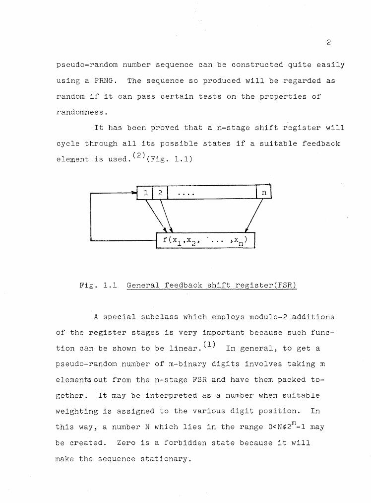
It has been proved that a n-stage shift register will

cycle through all its possible states if a suitable feedback

element is used. ( 2 )(Fig. 1.1)

,x ) n

Fig. 1.1 General feedback shift register(FSR)

A special subclass which employs modulo-2 additions

of the register stages is very important because such func­

tion can be shown to be linear. (l) In general, to get a

pseudo-random number of m-binary digits involves taking m

elements out from then-stage FSR and have them packed to-

gether. It may be interpreted as a number when suitable

weighting is assigned to the various digit position. In

this way, a number N which lies in the range O<N~2m-l may

be created. Zero is a forbidden state because it will

make the sequence stationary.

3

The numbers coming out from the FSR will be uni­

formly distributed in the range of (l,2m-l). Every number

(or possible state) in this range has equal probability of

occurance.

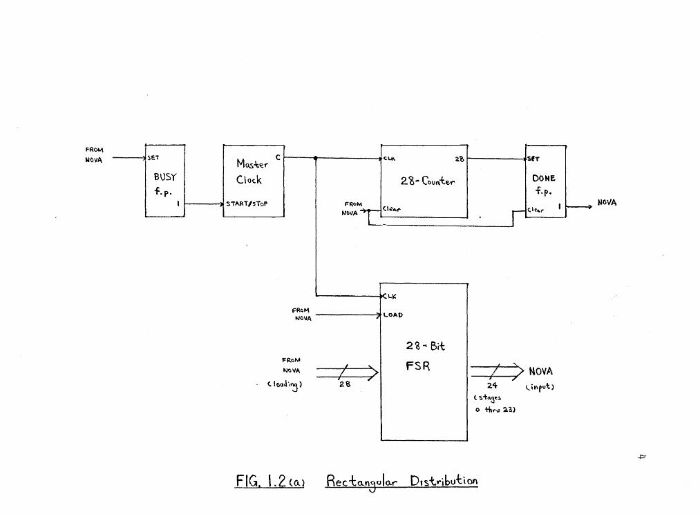
Repeated convolutions of a uniform distribution

will give rise to an approximation to a gaussian distri­

bution. C3 ) Convolution of two distributions corresponds

to finding the resultant probability density function of

the two independent random variables being added together.

Using convolution theory, the gaussian distribution in this

project is generated by adding twelve consecutive rect-

angular numbers together.

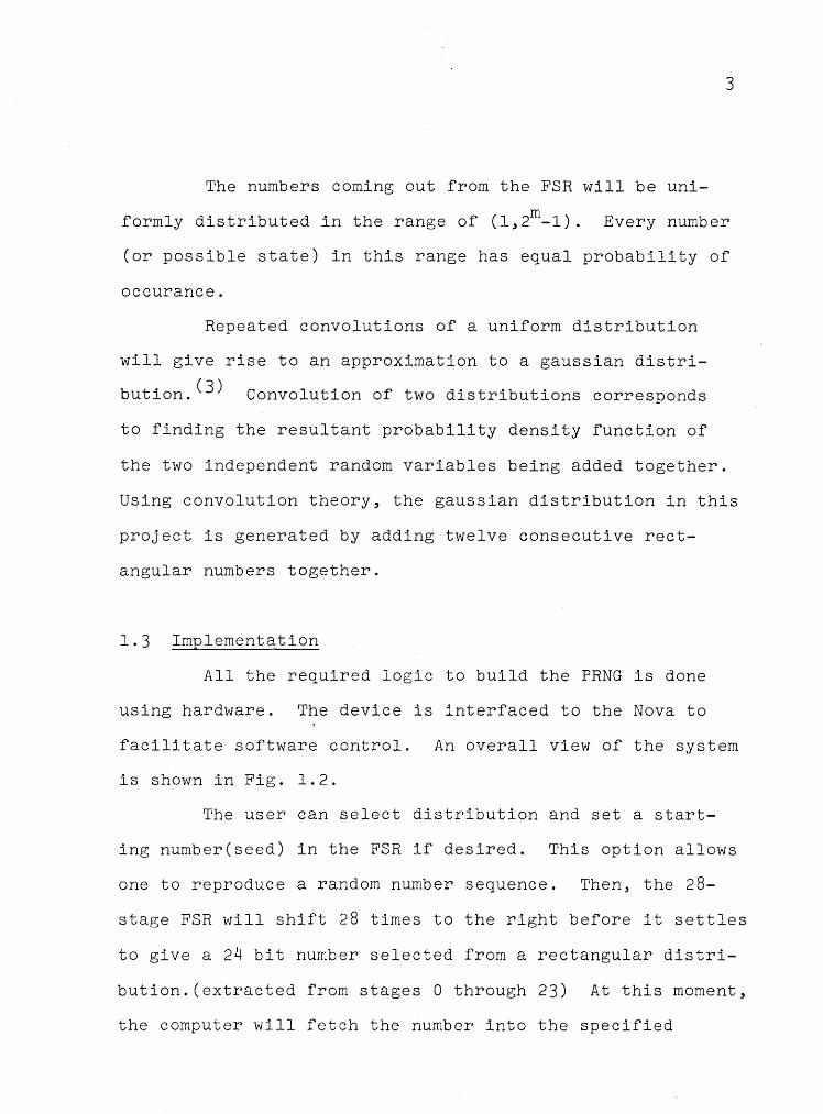
1.3 Implementation

All the required logic to build the PRNG is done

using hardware. The device is interfaced to the Nova to

facilitate software control. An overall view of the system

is shown in Fig. 1.2.

The user can select distribution and set a start-

ing number(seed) in the FSR if desired. This option allows

one to reproduce a random number sequence. Then, the 28-

stage FSR will shift 28 times to the right before it settles

to give a 24 bit number selected from a rectangular distri-

bution.(extracted from stages 0 through 23) At this moment,

the computer will fetch the number into the specified

FROM

WC>VA -" 5ET

BUSY

f.p.

'

MCAS-t~f' c

C\oc.k

~ S'TAAT/sToP

FReM NOVA

FrtcM

~VA

<. loQJi~)

FIG. \.2 <a.>

<;~ 2.~ Sf T

2. %- Coun*.e.,- DOME f.p.

FROM l I Nf>VA L .( €4'..t' Jc.leG.,.

NOVA

.... L~

-] l.OAO

2i-. Bit

FSR t >NOVA l > z I ' 2.e 2.4 urirot>

(. '$t~.'.3~~ 0 +hN 23)

..J:::-

Rec 1:a.n3ula.r D1s-lr&buhon

Start

Start the generator.

Set G = 0.

Bring in the rect.

no. R & restart the

generator.

G = G+R

G is the required

gaussian no.

Finish

5

Fig. l.2(b)

Gaussian

Distribution

6

accumulators.

If a gaussian number is selected, twelve constcutive

rectangular numbers from the FSR will be added together to

give a sample from a gaussian distribution. The addition

is done by software in the Nova. Only 20 bits from the 24-

bit rectangular sample(stage 4 through 23) are used in each

addition.

Rate of clock pulse used is about 2.5 Mhz. It would

mean a minimum of 11.2 microseconds is needed to generate a

sample from a rectangular distribution.

The reason to shift the FSR 28 times is to ensure

that maximum length can be obtained while inter-correlation

between consecutive numbers is minimized.

7

CHAPTER 2

HARDWARE DESIGN

The purpose of the hardware is to generate uniformly

distributed numbers. Using this source, gaussian distributed

numbers can be created through addition.

2.1 Rectangular distribution

Detailed hardware diagrams are shown in Fig. 2.1 to

Fig. 2.5.

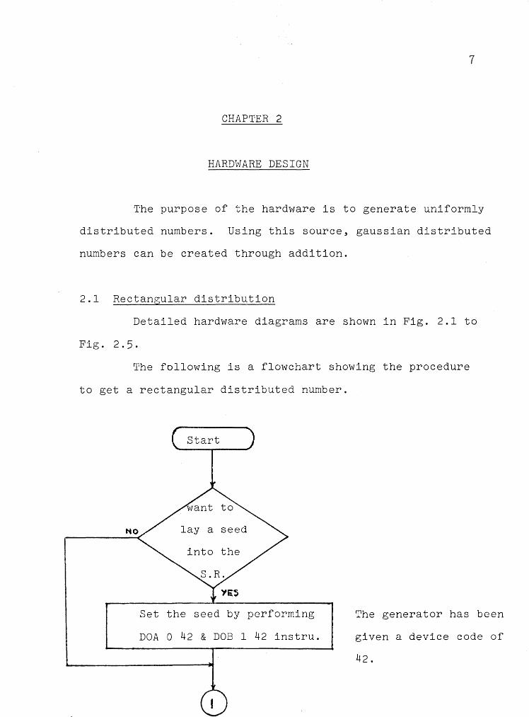
The following is a flowchart showing the procedure

to get a rectangular distributed number.

Start

Set the seed by performing

DOA 0 42 & DOB 1 42 instru.

The generator has been

given a device code of

42.

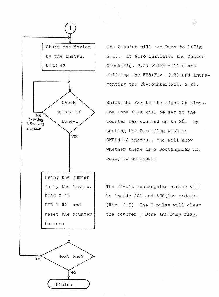
Start the device

by the instru.

NIOS 42

Bring the number

in by the instru.

DIAC 0 42

DIB 1 42 and

reset the counter

to zero

8

The S pulse will set Busy to l(Fig.

2.1). It also initiates the Master

Clock(Fig. 2.2) which will start

shifting the FSR(Fig. 2.3) and incre­

menting the 28-counter(Fig. 2.2).

Shift the FSR to the right 28 times.

The Done flag will be set if the

counter has counted up to 28. By

testing the Done flag with an

SKPDN 42 instru., one will know

whether there is a rectangular no.

ready to be input.

The 24-bit rectangular number will

be inside ACl and ACO(low order).

(Fig. 2.5) The C pulse will clear

the counter , Done and Busy flag.

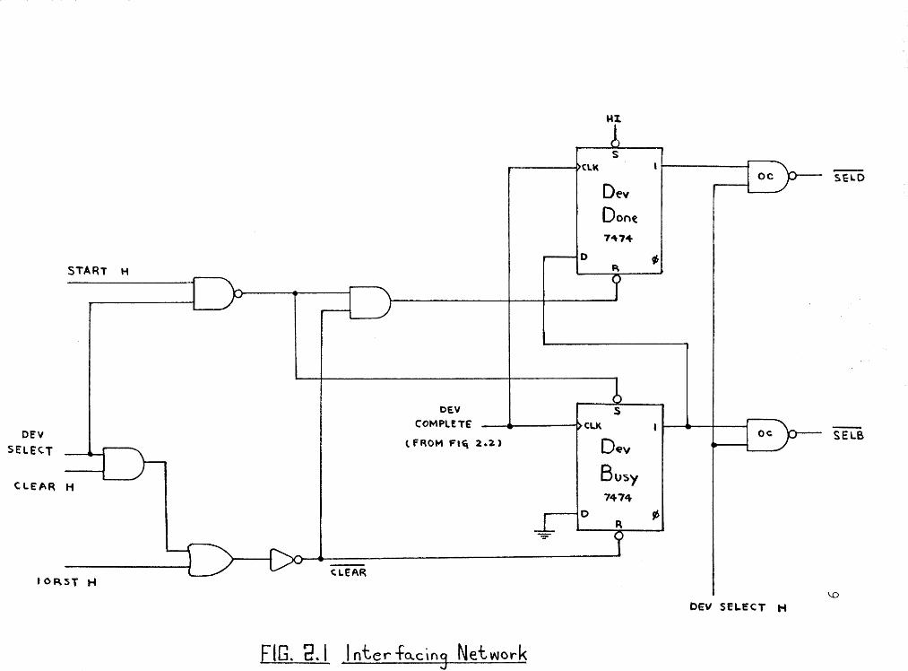
OcV SE'LEC.T

CLEAR H

t ORST H

DEV COMPLETE --·----

l FROM Flq 2.2 >

CLEAR

FlG. 2.1 Inter fo..c\n~ Network

s ---l>CL.k

0

o~v

Busy 7474

SELS

,s

\.0

DEV SELECT H

Ma.sler Clock

SUSYt~} ~IA -, _ lB

12Q~ 2Q

2A I~ 2.B

I 3 lK

sv I I

TIMIN§ ELEMENTS

Re 8K c = 33pf Ft-e~. ~ 2.5 Mh~

FIG. Z.2 TiM"1n3 0Nice

28- Counter

l)CL~

rleN T ~ p 6

I

~LMD sv

C:LEA~ CAR.RY illM C.F~M Flq. 2.l)

s C.LK

7

~:r + 7 sv 6

K q

'}- OEV COM PLETe:

f--l 0

Loo.clin§ L~ le.

lB TIMIN§ HEME~T.S 7

L0-41A 4 lR a 6.gK

I '<:-:. '0 pf

lQ-12.A 2 2R~ 8K

3 2C. ~ lO pf

HI --f2S 2Q

PA TOA

Q. .. DE\/

~ELE<.T I l -- L-.l -......... -- r I \---

Cb

~ -

I -

OA'ToS ....___.

0 I FROM r:1~. l.2

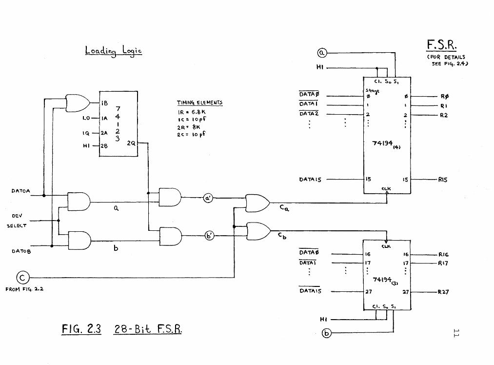
FIG. 2.3 28- Bit F.S-1i

a.\...--------, ..........

Ht --~~~~-,r--i

DATA¢

OAiAI

OAiA2.

OATAlS

DATA¢

CATA\ .

DATA\$

Cl. So S,

s~1~ -----,0

-------42.

"7419\4,

I'S Ct.\(

<.LK

16

17 . . . . . 74l~4<3,

21

c.1. S 0 S, I

' I

HI

rb) I

F.S.R. C FOR OETAlLS

SEE Fl<"=t. 2.1-)

¢E~~ ~'

2 R2

1s 1 RlS

•6F~'G 17 R.'7 .

171Rl.7

f-l f-l

2 3

4 s 6 7

8

' 10 ll

\K _A.AAA.a. ,.,.,,,,..,

----

Oo..t~ ; -

FROM Fl<l- 2.3

4-

s 6 ..,

'O 9

lO

ll

I --

b

@

@-J

"'

l_ ' [ If

c. '· -S.tt Q ..

A 8 e c (,,

D 0

<L\< So s, ::.-

r .I ..I

~ R=<•· $~R. QA A & '3 c. (.

0 0

<Lt< c::;. 5t ::I

::r ::J

ffju. s~ ~ ~ g 6 c. c. 0

0 CLK s. Si

:I ..J

::I H: c:.1. ~~ QA A 8 6 <;. c 0 0 Cl.K 'Sc, s,

..I :.I

ft~~ ~~ Q. A 6 s (. (. 0

0 CL..K So s,

I ..l J:

f-lj ~L'• ~R QA

A g 6 (;.

(..

D 0 C.L.I<. ~ . ~.

T ..l

_[

•ftt•· ~~ QA A 8 s c:. c. 0

0 IC:.\..K So s. I

I l 7 x 74194

_....

---

---

-

-

4 s (,

7

lO

II

l 2.

\~

l"t

lS

20 2..l

22 .2.3

2"\

2.5

2.6

R '2. 7

12

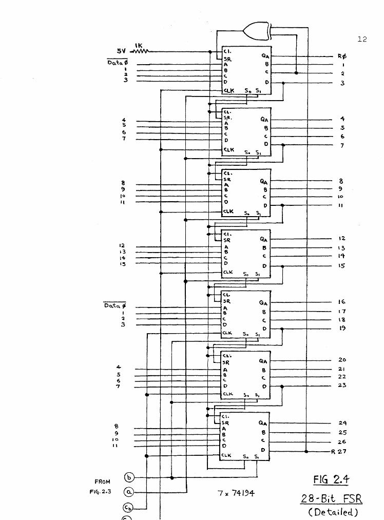
FIG 2.t

2 8 -- Bi t FSR ta.ii ed.) (De

13

( fRoM Flq. 2.3)

R/ OATAlS

t>AT IS

Oi:V

se1..&<T ~1'~oBE

DA'Tl A

Ri ~

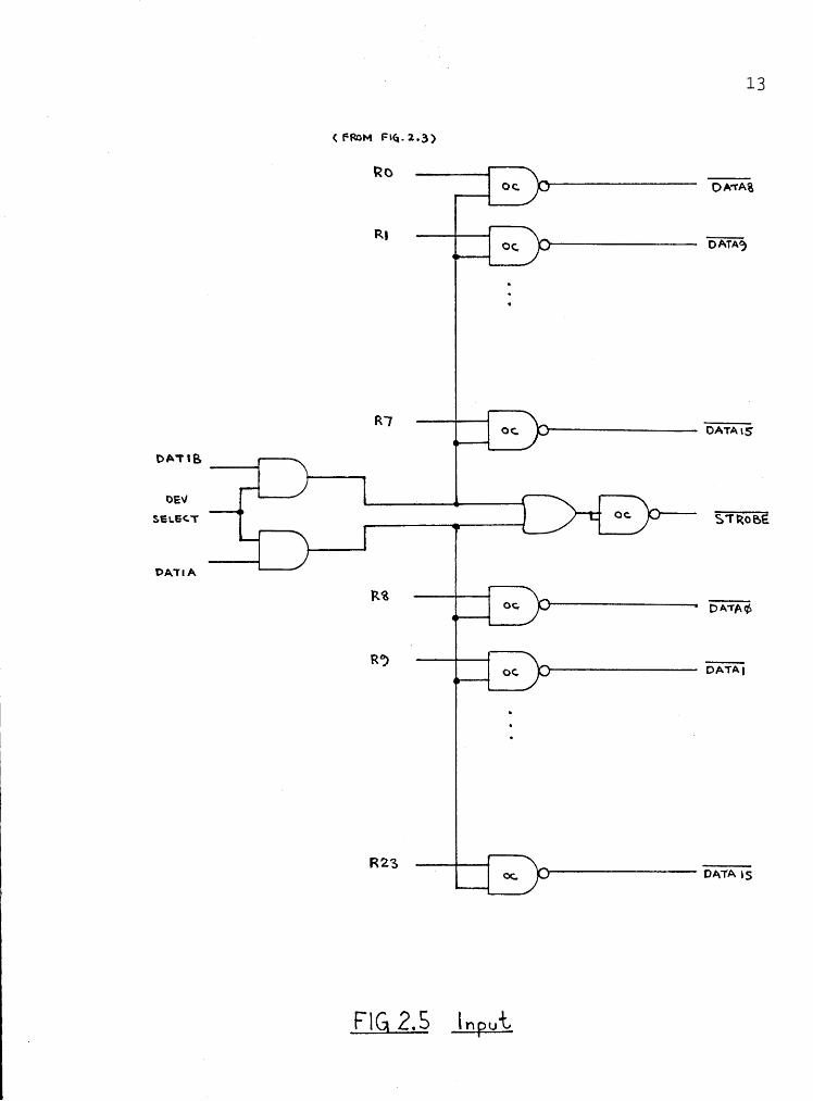
FlG 2.5

number:

There are three stages in getting a rectangular

1. Laying of a seed (Output from computer)

2. Generation by shifting the FSR 28 times to the

right.

3. Input (Input to computer)

In each step the command is coming from the Nova.

Laying of a seed

The random sequence can start at a certain state by

setting a number into the FSR at the beginning. The number

should be inside ACl and ACO(lower order) before the follow­

ing instructions are performed:

DOA 0 42

DOB 1 42

These two instructions will load

bit 0 through 15 of ACO into stage 0 through 15 of

FSR(Fig. 2.3). and bit 0 through 11 of ACl into

stage 16 through 27 of FSR.

Null state is avoided by software described in

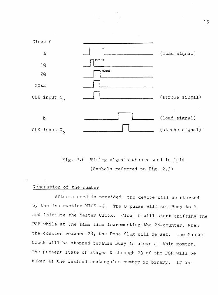
chapter 3. Fig. 2.6 shows a timing diagram of the signals

during loading.

14

Clock C

a

lQ

2Q

CLK input Ca

b

CLK input Cb

_J __Jl~'o_o_n_~~~~~~~~~~­

___n~·-~o_n_~~~~~~~~~

_n ___ _

_n~---

(load signal)

(strobe singal)

(load signal)

(strobe signal)

Fig. 2.6 Timing signals when a seed is laid

(Symbols referred to Fig. 2.3)

Generation of the number

After a seed is provided, the device will be started

by the instruction NIOS 42. The S pulse will set Busy to 1

15

and initiate the Master Clock. Clock C will start shifting the

FSR while at the same time incrementing the 28-counter. When

the counter reaches 28, the Done flag will be set. The Master

Clock will be stopped because Busy is clear at this moment.

The present state of stages 0 through 23 of the FSR will be

taken as the desired rectangular number in binary. If an-

other number is required, the whole generating procedure may

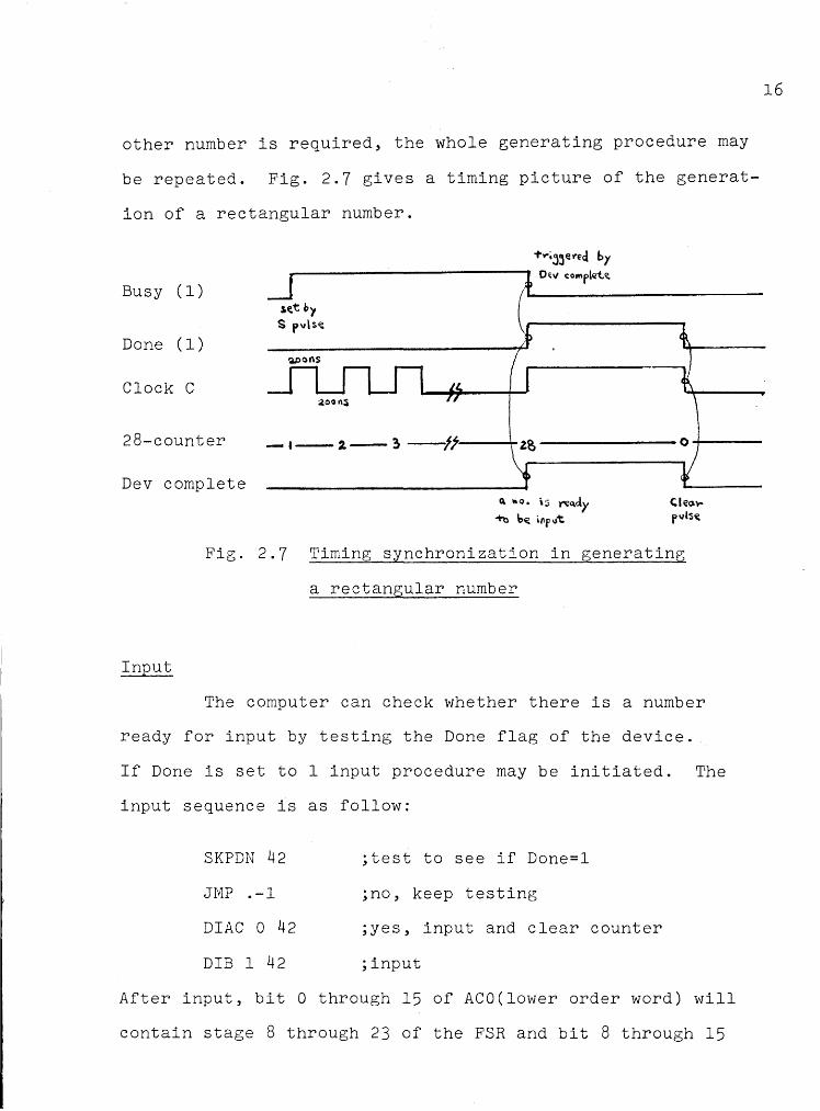
be repeated. Fig. 2.7 gives a timing picture of the generat-

ion of a rectangular number.

Busy (1)

Done (1)

Clock C

+'f"~J~e""ecl by

__J------------------~l __ o_~~-c_o_mr_l<rt.--~---------------­i(t b'1

S pv\s~

28-counter - ·--,. _ ~ __ .,,. _____ ....,. ---------0-+----

Dev complete

Input

" •o • \~ ~'\c.ly

-t-o b~ '"r~t

Fig. 2.7 Timing synchronization in generating

a rectangular number

The computer can check whether there is a number

ready for input by testing the Done flag of the device.

If Done is set to 1 input procedure may be initiated. The

input sequence is as follow:

SKPDN 42

JMP .-1

DIAC 0 42

DIB 1 42

;test to see if Done=l

;no, keep testing

;yes, input and clear counter

;input

After input, bit 0 through 15 of ACO(lower order word) will

contain stage 8 through 23 of the FSR and bit 8 through 15

16

17

of ACl will contain stage 0 through stage 7 of the FSR.

2.2 Gaussian distribution

The gaussian number is created by adding twelve

consecutive rectangular numbers together. Details of

generation is depicted in Fig. l.2(b). Instead of adding

the whole 24 bit number, only the least significant 20 bits

are added together each time. It is done to suit the float­

ing point notation of the Nova. Hence, the addition result

will never exceed 24 bits in length.

CHAPTER 3

SOFTWARE CONTROL

The PRNG can be called from a Basic or a Fortran

environment under the Real-time Disk Operating System(RDOS)

of the Nova.

3.1 Fortran callable subroutines(5, 5 ,7)

Three subroutines have been implemented in the

Fortran environment. Their function and calling sequence

are as follow.

(a) CALL RAND(X,XMEAN,STD) for rectangular distribution.

where X = returned rectangular distributed number.

XMEAN = mean of the distribution.

STD = standard deviation of the distribution.

X,XMEAN and STD are numeric variables.

(b) CALL RANG(X,XMEAN,STD) for gaussian distribution.

Everything will be similar to (a) except that X will

be the returned gaussian distributed number.

(c) CALL SEED(S) for laying a seed in the generator.

where S = the starting value(seed) which would be

loaded into the FSR of the generator. Arbitrary seed

will be used if S is zero.

S is a numeric variable.

18

A listing of each subroutine is attached at the

end of the chapter.

3.2 Basic callable subroutines(5, 6 ,7)

19

Similar to the Fortran calls, there are three options

available in BasicG.

(a) CALL 5,X,M,S for rectangular distribution.

where X = returned rectangular distributed number.

M = mean of the distribution.

S = standard deviation of the distribution.

Xis a numeric variable. Mand Sare numeric expressions.

(b) CALL 6,X,M,S for gaussian distribution.

Everything will be similar to (a) except that X will

be the returned gaussian number.

(c) CALL 7,S for laying of a seed.

where S = seed which would be loaded into the FSR of

the generator. Arbitrary seed will be used

if S is zero.

S is a numeric expression.

A listing of each subroutine is not provided because

it is very similar to the corresponding Fortran subroutine

except for the linkage between Basic and the assembly lang­

uage subroutine.

20

_;*********~******************************************************

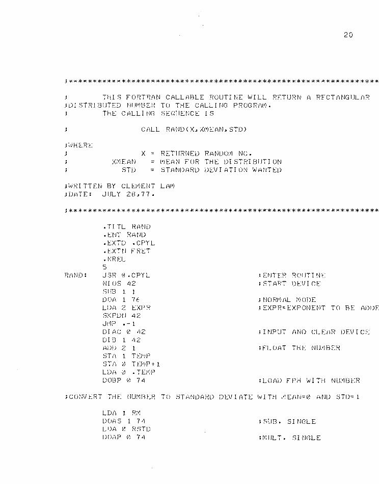
THIS FORTRAN CALLl-'iBLE ROLJTI NE WILL RETlHW A RECTMJGULAR _; UI STRI BUTED ~JI JMBEi~ TO THE CALL I NG PROGRAM. _; TH~ CALLING S~QUENCE IS

CALL RANDCX,XMEAN,STD)

;tvHERE X = RETl JRNED RANDOM NO.

; XMEMJ = fYiEMJ FOR THE DI STf~I BUTI ON STD = STMJDARD DEV I ATI ON \,./ANTED

;WRITTEN BY CL8<JENT LAM ; DATE : J UL Y 2 8 , 7 7 •

_;****************************************************************

RMJD:

• TI TL RAND .ENT RAND .EXTD .CPYL .EXHJ FRET • NREL 5 JSR l0! • CPY L NI OS L12

st 1s 1 1 DOA 1 76 LD~\ 2 EXP R 5KPDN 42 Jr11P .-1 DI AC V, IQ

DIB 1 42 1-mu 2 1 ST?\ 1 T l::(YJ p

STA 0 TEMP+ 1 LDl-1 (I) • T EJtlP DOBP Ci} 7 Lj

; ENTER ROlJTI NE ;STA"S'T DE\JICE

_;NORM 1'\L (YJ ODE ; EXPR=EXPONENT TO BE ADDE

_;INPUT AND CL Et4H DEV I CE

;FLOAT THE NU~BER

; LOl'\lJ FPH :_..11 TH NUr<JBE:R

_;CONVERT THE NUMB t:R TO ST MJDMW DEV I ATE t.v I TH ,•1 EM~-= v; I-HJD ~)TD= 1

LOA 1 RM DO?\ S 1 7 /4

LDA e HSTD DOi~P 0 7 4

;SUB. SINGLE

;(YJ!JL T. SI ~JGLE

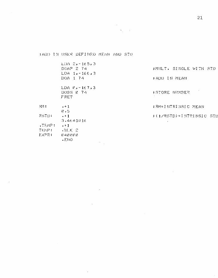
; I~ U D I t'J LI SE R DEF I N ED fYi E Ar'J A ND ST))

RM:

RSTD:

L D?~ 2 _, - 16 5 _, 3 DOAP 2 74 LDA 1.,-166.,3 DOA 1 7 Li

LOA 0 _, - lt 7 _, 3 DOBS 0 74 FRET

• + 1 0.s • + 1 3 • 46 Lt rn 16

. T EJYi p : • + 1 T£(YJP: • BLK 2 L<PR: 0Lirt0rt~

.END

21

;MIJLT. SI~JGLE WITH STD

;ADD IN MEAN

; STORE NUMBER

JRM=INTRINSIC MEAN

J(l/RSTD>=INTRINSIC STD

22

;**************************************************************~

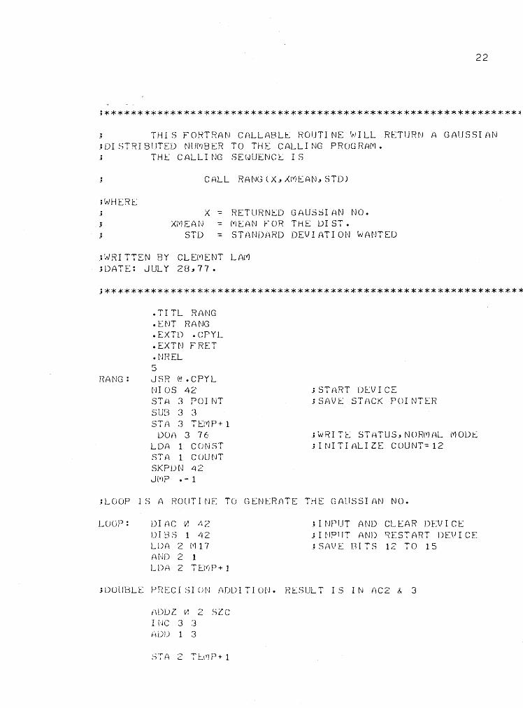
_; THIS FORTRAN C{\LLABLE ROUT! NE l,.Jl LL RE:TURN A GAUS SI M.J ;DISTRIBUTED NlJ('t'18ER TO THE CALLING PROGHAM. _; THE CALLING SEWUENCE IS

_; CALL RANGCX,XMEAN,STD)

;WHERE _; X = RETURNED GAUSSIAN NO. ; XMEAN M~AN FOR THE DIST. ; STD : STAr-JDARD DEV I ATI ON WANTED

;WRITTEN BY CLEMENT LM1 ;DATE: JULY 28,77.

;***************************************************************

RANG:

• TI TL RMJG .ENT RANG .EXTD .cPYL .EXTN FRET .NHEL 5 JSR @.CPYL r-JI OS 42 STf.\ 3 POI NT SUB 3 3 ST/.\ 3 T EtYJ P + 1

DOii 3 76 LDA 1 CCJNST STA 1 CUUNT SKPUN 42 .J(YJP • - 1

; ST 1-\RT DE:V I CE ;SAVE: STACK POINTER

_; W R I T I:: ST iH U S, N 0 RM HL M OLYt= ;INITIALIZE COUNT=12

;LOOP IS A ROUTINE TCJ GEf'JERf\TE THE GALISSI /.\N NO.

LOOP: ur nc 0, 1-12

IJIB:S 1 42 LUA 2 M17 AND 2 1 LDI~ 2 TH'iP+ 1

; INPUT AND CLEAR DEV I CE _;I ~JPI IT AND \\EST ART l)f\I I CE ;SAVE BITS 12 TO 15

;DUlJBLE PRECISION /\DDITIC_HJ. r:E:.SULT rs IN AC2 & 3

f\DUZ ~ 2 SlC I t~C 3 3 1-\UU 1 3

DSL: CO!WT ._MP LOOP

LDA 1 EXPG {\DD 1 3 STA 3 TEMP LDA 0 • TEJYJP DOBP 0 ?'-!

23

; COUNT:-= 0 ? ; ~JO_, C 0 NT I NU E T 0 ADD

;YES., FLOAT THE GAllSSIMJ ~JO.

; ADD IN EXPONEt'H

;LOAD SINGLE

; CONV Ern TO ST Al'JDARD JJE\J I ATE., rt/-= 0 & STD-= 1 ; I NTRI NSI C STD::: 1

LDA 1 GM DOAS 1 74 ;SUB SING

; ADD I f~ USER DEF I ['JED lYl EAN f.\ ['JD STD

GM:

POINT: CONST: COUNT: \"'l 17 :

EXPCJ: • TE!YJP: TEMP:

LDA 2 POINT LOA 3,-165.,2 DOAP 3, 7 LJ

LI)A 1,-J.t.l_,2 DOA 1 7 4

LD?\ 2 _, - lf.,; 7 _, 2 DOB S 2 7 4 FRET

• + l 6.0

"' 14 ~

17 0LJ0LJ00

• + 1 v, ~

.END

h•1l IL T SI NG

; ADD SI r,JG

; STORE SI !'1GLE _;RETURN

;GM=INTRINSIC MEAN OF DIST

24

_;*****************************************************************

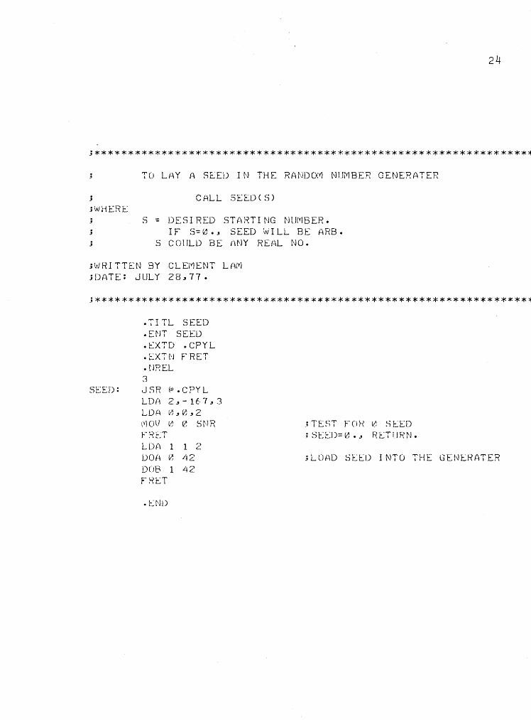
TO LAY A SE:ED IN THE RANDOM NUMBER GENER ATER

_; CALL SEED(S) HvHERE _; S : DESI RED START! NG NlHYlBER. _; IF S=0., SEED WILL BE ARB. _; S COULD BE MJY REAL t'-JO.

;WRITTEN BY CLEMENT LAM ;DATE: JULY zg,77.

_;****************************************************************~

SEED:

• 7I TL SEED • HJT SEED .£XTD .CPYL .EXTN FRET • tJREL 3 JSR (al .cPYL L D /\ 2 , - 16 7 , 3 LD?\ 0,v,,2 \YJ 0 \J L~ l?. S N R FRET LOA 1 1 2 !JOH er, A 2 DOB 1 1-J2 FRET

• UJD

_;TEST FOH 0 SEED _;SEED= 0., RETURN.

;LOAD SEED INTO THE GENEHATER

CHAPTER 4

TESTS AND OBSERVATION

The PRNG was subjected to three statistical tests.

They were

(i)

(ii)

(iii)

Frequency test

Correlation test

d 2-test

4.1 Frequency test(l,3)

In this test, one divides the possible existence

interval of the numbers in equal non-overlapping intervals

and tallies the amount of numbers in each interval. The

probability density function and the distribution function

of the generated numbers can be obtained by examining the

tally in each interval.

4.1.1 Rectangular distribution

The interval examined was (0,1). It was divided

into 1000 channels or bins and 10 6 numbers were sampled

and sorted into the corresponding channel.

If the numbers are uniformly distributed in (0,1),

then one would expect each channel to contain lOOO±JlOOO

numbers. If the numbers of elements inside a channel is

25

26

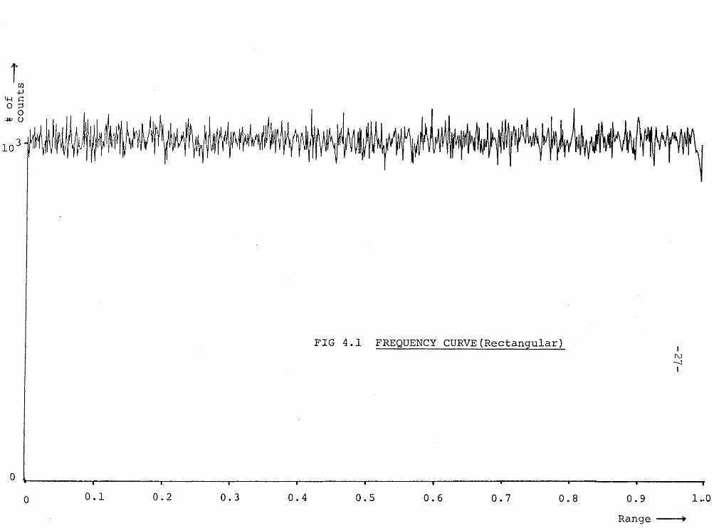
plotted against the channel number, a horizontal line should

be obtained.

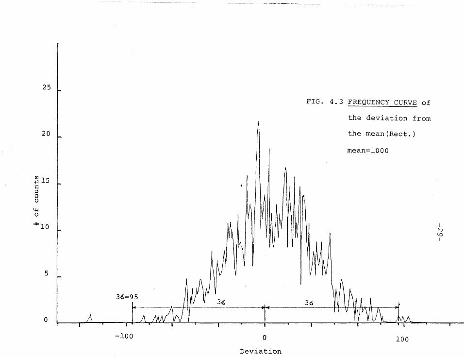
Fig. 4.1 shows the actual frequency curve obtained

by the above mentioned method. It is quite a close approxi­

mation of the uniform distribution. Further look at Fig. 4.3

indicates that the distribution obtained is statistically

acceptable. The normal standard deviation is equal toJlOOO.

It can be seen that all non-zero channels lie within the 36

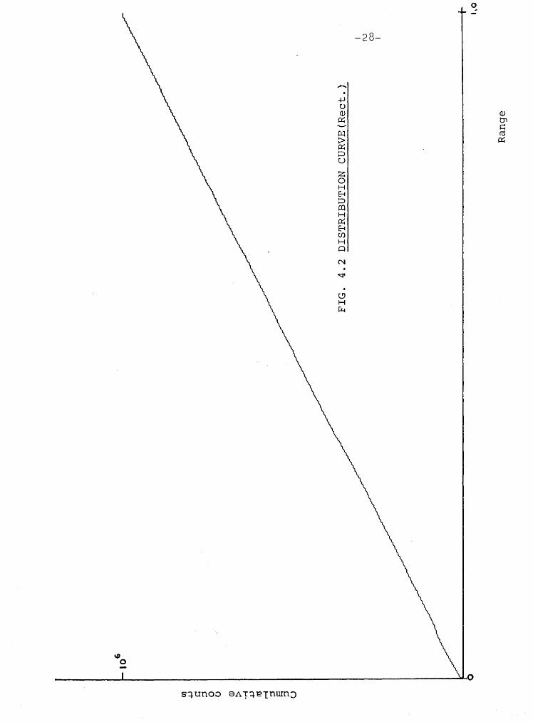
limit. The integral distribution curve shown in Fig. 4.2

further reinforces the indication that the distribution so

obtained is uniform.

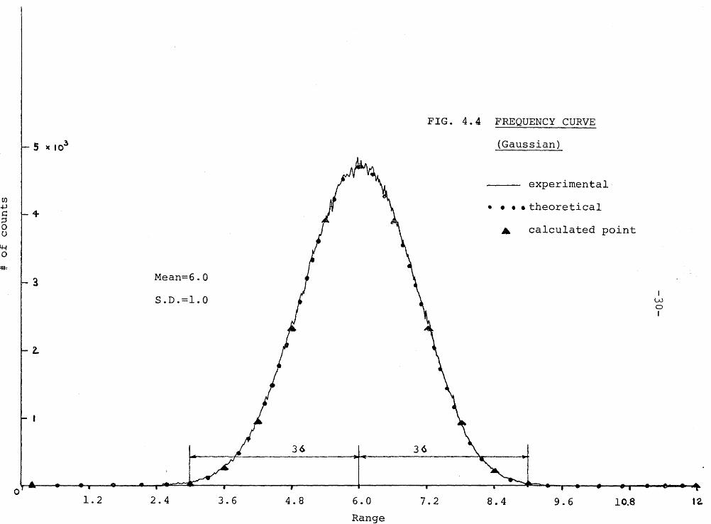
4.1.2 Gaussian distribution

The interval being examined was (0,12). It was again

divided into 1000 channels and io 6 numbers were sampled.

From Fig. 4.4, the frequency curve obtained from plot-

ting the tally in each channel against the channel number

appears like a gaussian distribution. Almost all counts are

inside the 36 limit. For comparison the analytical description

of a gaussian distribution is plotted on the same graph. This

reveals good agreement suggesting the random source is stat-

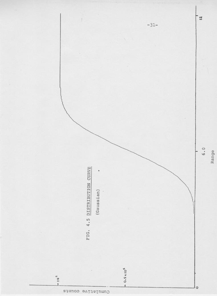
istically acceptable. The integral distribution curve in

Fig. 4.5 further supports this inference.

i CJ) .µ

::~~~~}~1~~~w~~~~~-~~

FIG 4.1 FREQUENCY CURVE(Rectangular)

0

0 0.1 0.2 0.3 0.4 0.5 0.6 0.7 0.8

~

I ('\)

-J I

0. 9 1..0

Range --

0

-28-

~ . ~ u w ill ~ ~

~ ~ m > ~ ~ ~ u z 0 H 8 ~ m H ~ 8 00 H Q

("I

~

~ H ~

25

FIG. 4.3 FREQUENCY CURVE of

the deviation from

20 the mean {Rect.)

mean=lOOO

.B 15 ~ ~ 0 0

4-f 0

'* 10 I lA I I 11 I U II\ 111 f I II ii 11 I I I I\) \.()

I

5

36=95 3~ 36

0

-100 0 100

Deviation

en .µ ~ :::l 0 {J

~ 0

#:

0

FIG. 4.4 FREQUENCY CURVE

5 -10~ (Gaussian)

i- +

I

3 Mean=6.0

S.D.=1.0

2.

36

1. 2 2.4 3.6 4.8 6.0

Range

36

7.2

experimental

• • • •theoretical

• calculated point

8.4 9.6 10.8

I w 0 I

12.

32

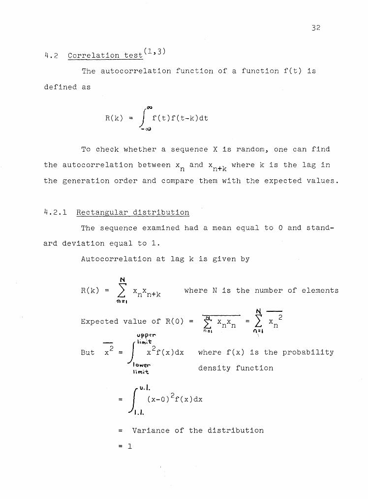
4.2 Correlation test(l,3)

The autocorrelation function of a function f (t) is

defined as

00

R(k) = ~ f(t)f(t-k)dt -ca

To check whether a sequence X is random, one can find

the autocorrelation between xn and xn+k where k is the lag in

the generation order and compare them with the expected values.

4.2.l Rectangular distribution

The sequence examined had a mean equal to 0 and stand-

ard deviation equal to 1.

Autocorrelation at lag k is given by

N

R(k) = 2 xnxn+k where N is the number of elements

'1l ='I

N

~ Expected value of R(O) = x x n n upper

But x2

= J ""':2r (x) dx

lower linfrt

n:a

where f (x) is the probability

density function

= (x-o) 2f(x)dx ju.I.

I.I.

= Variance of the distribution

= 1

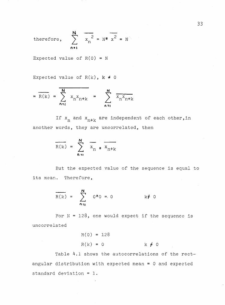
N therefore, I 2

N* x 2 N x = = n

n:a

Expected value of R(O) = N

Expected value of R(k), k ~ 0

N

= R(k) = "' x x L n n+k =

If xn and xn+k are independent of each other,in

another words, they are uncorrelated, then

N

R(k) = ~ x x .L n * n+k I\ -:1

33

But the expected value of the sequence is equal to

its mean. Therefore,

N

R(k) = L O*O = 0 kl 0

"::a

For N = 128, one would expect if the sequence is

uncorrelated

R(O) = 128

R(k) = 0 k f 0

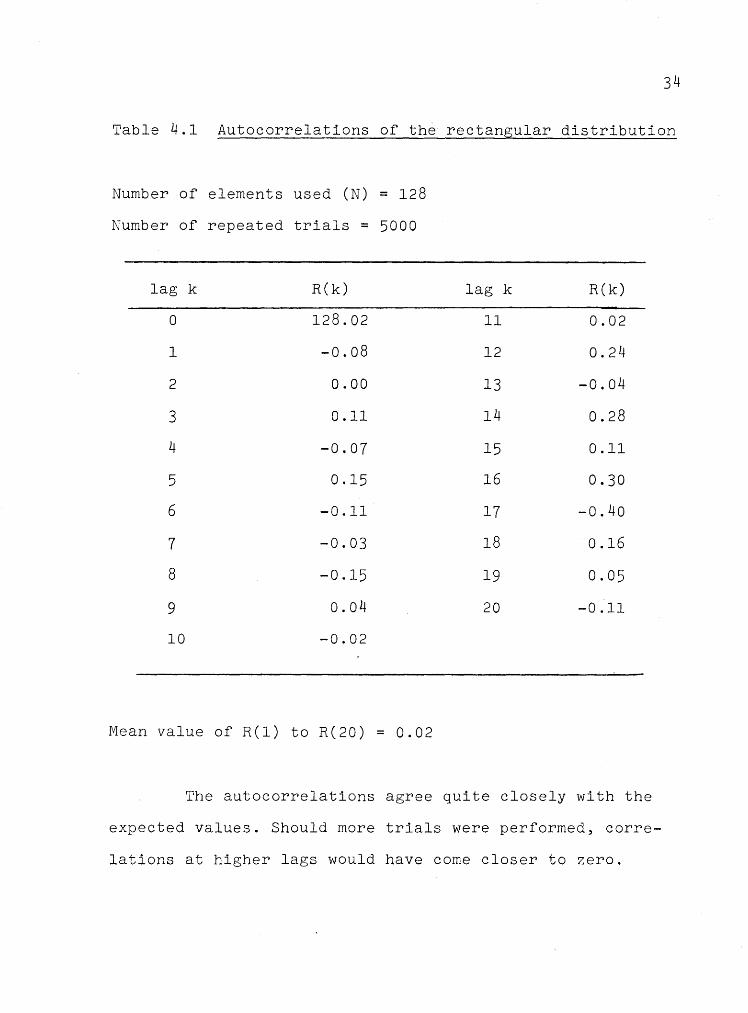
Table 4.1 shows the autocorrelations of the rect-

angular distribution with expected mean = 0 and expected

standard deviation = 1.

34

Table 4.1 Autocorrelations of the rectangular distribution

Number of elements used (N) = 128

Number of repeated trials = 5000

lag k R(k)

0 128.02

1 -0.08

2 0.00

3 0.11

4 -0.07

5 0.15

6 -0.11

7 -0.03

8 -0.15

9 0.04

10 -0.02

Mean value of R(l) to R(20) = 0.02

lag k R(k)

11 0.02

12 0.24

13 -0.04

14 0.28

15 0.11

16 0.30

17 -0.40

18 0.16

19 0.05

20 -0.11

The autocorrelations agree quite closely with the

expected values. Should more trials were performed, corre­

lations at higher lags would have come closer to zero.

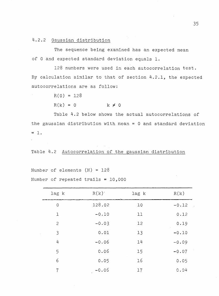
4.2.2 Gaussian distribution

The sequence being examined has an expected mean

of 0 and expected standard deviation equals 1.

35

128 numbers were used in each autocorrelation test.

By calculation similar to that of section 4.2.1, the expected

autocorrelations are as follow:

R(O) = 128

R(k) = 0 k ~ 0

Table 4.2 below shows the actual autocorrelations of

the gaussian distribution with mean = 0 and standard deviation

= 1.

Table 4.2 Autocorrelation of the gaussian distribution

Number of elements (N) = 128

Number of repeated trails = 10,000

lag k R(k)- lag k R(k)

0 128.02 10 -0.12

1 -0.10 11 0.12

2 -0.03 12 0.19

3 0.01 13 -0.10

4 -0.06 14 -0.09

5 0.06 15 -0.07

6 0.05 16 0.05

7 -0.06 17 0.04

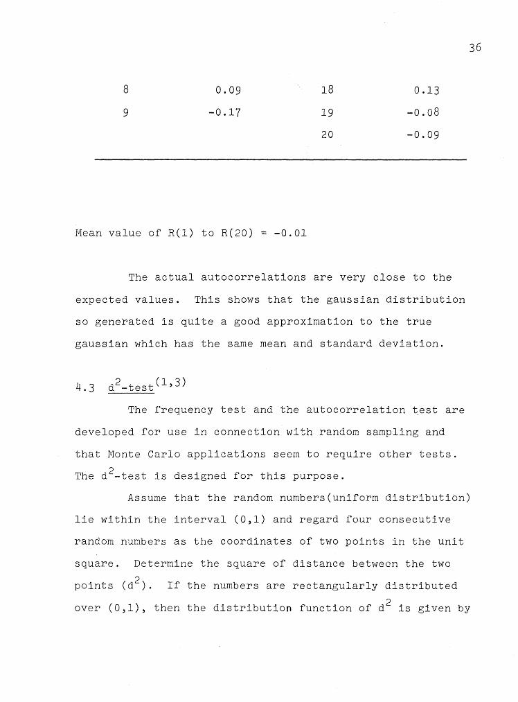
8

9

0.09

-0.17

Mean value of R(l) to R(20) = -0.01

18

19

20

0.13

-0.08

-0.09

The actual autocorrelations are very close to the

expected values. This shows that the gaussian distribution

so generated is quite a good approximation to the true

gaussian which has the same mean and standard deviation.

The frequency test and the autocorrelation test are

developed for use in connection with random sampling and

that Monte Carlo applications seem to require other tests.

The d 2-test is designed for this purpose.

36

Assume that the random numbers(uniform distribution)

lie within the interval (0,1) and regard four consecutive

random numbers as the coordinates of two points in the unit

square. Determine the square of distance between the two

points (d 2 ). If the numbers are rectangularly distributed

over (0,1), then the distribution function of d 2 is given by

37

ll'S 2

- 8/3s 2 + s 4;2 when 2

s ~ 1

{ 2 2 2)s 2 + 4(s 2 1

+ 8/3(s 2-1) 312 1/3 + (Tr - )~ p(d ~ s ) = -1

4 4 2 -1 - s /2 - s *sec s when 2 l< s ~ 2

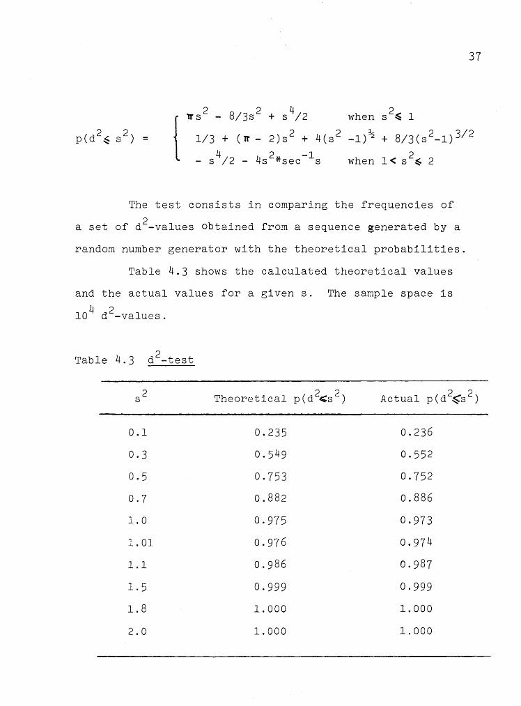
The test consists in comparing the frequencies of

a set of d 2-values obtained from a sequence generated by a

random number generator with the theoretical probabilities.

Table 4.3 shows the calculated theoretical values

and the actual values for a given s. The sample space is

10 4 d

2-values.

Table 4.3

2 s

0.1

0.3

0.5

0.7

1. 0

2 d -test

1. 01

1.1

1. 5

1. 8

2.0

0.235

0.549

0.753

0.882

0.975

0.976

0.986

0.999

1. 000

1. 000

2 2 Actual p(d ~s )

0.236

0.552

0.752

0.886

0.973

0.974

0.987

0.999

1. 000

1.000

38

As one can see, the experimental results agree closely

with the theoretical values.

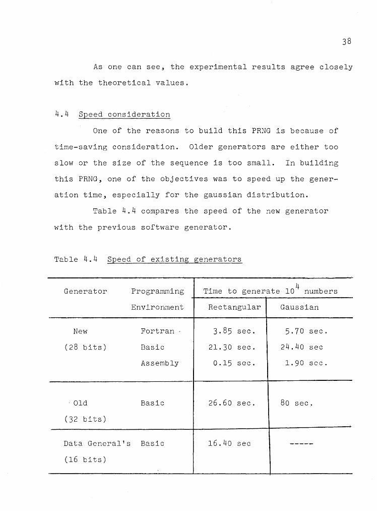
4.4 Speed consideration

One of the reasons to build this PRNG is because of

time-saving consideration. Older generators are either too

slow or the size of the sequence is too small. In building

this PRNG, one of the objectives was to speed up the gener-

ation time, especially for the gaussian distribution.

Table 4.4 compares the speed of the new generator

with the previous software generator.

Table 4.4 Speed of existing generators

Generator Programming Time to generate 4 10 numbers

Environment Rectangular Gaussian

New Fortran - 3.85 sec. 5.70 sec.

(28 bits) Basic 21. 30 sec. 24.40 sec

Assembly 0.15 sec. 1. 90 sec.

Old Basic 26.60 sec. So sec.

(32 bits)

Data General's Basic 16.40 sec -----

(16 bits)

39

It can be seen that a big improvement in speed

is achieved for the gaussian distribution. As a matter of

fact, the generator is capable of generating one rectangular

number in about 11.2 microseconds. All the time has been

wasted in program linkage and system commands when working

in the high level language environment.

The generator provided by Data General is faster than

the existing ones. However, it does not produce samples which

obey any of the randomness tests. It is not desirable when

numbers with a greater degree of randomness are required.

40

CHAPTER 5

CONCLUSION

The rectangular and gaussian distributions produced

as a result of the PRNG have been proved to be a very good

approximation of the corresponding theoretical distributions

judging from the test results. It is relatively inexpensive

and easy to construct such a PRNG using shift registers.

When cost and time are the main concern, this type of PRNG

is most suitable.

The following points are worth mentioning.

1. The clocking frequency could be increased considerably

to speed up the generation time. The fact that a large

portion of the time in getting a number is wasted in

system linkage(Table ~.4) makes it quite meaningless to

increase the clocking frequency unless the user is will­

ing to work in an assembly language environment.

2. The gaussian distribution can be generated by hardware.

The whole circuitry will become a lot more complex. As

long as useful instructions can be squeezed in between gen­

eration time of a rectangular number, the time saved is not

significant. In fact, the required hardware to generate the

gaussian distribution has been implemented and it only im­

proved the speed in a Fortran environment marginally while

no significant improvement was observed in Basic. However,

the required circuitry became tw~ce as complex as that for

the rectangular distribution. In the light of maintenance

of the hardware, software generation has been implemented

for the generation of normally distributed variables.

41

APPENDIX A

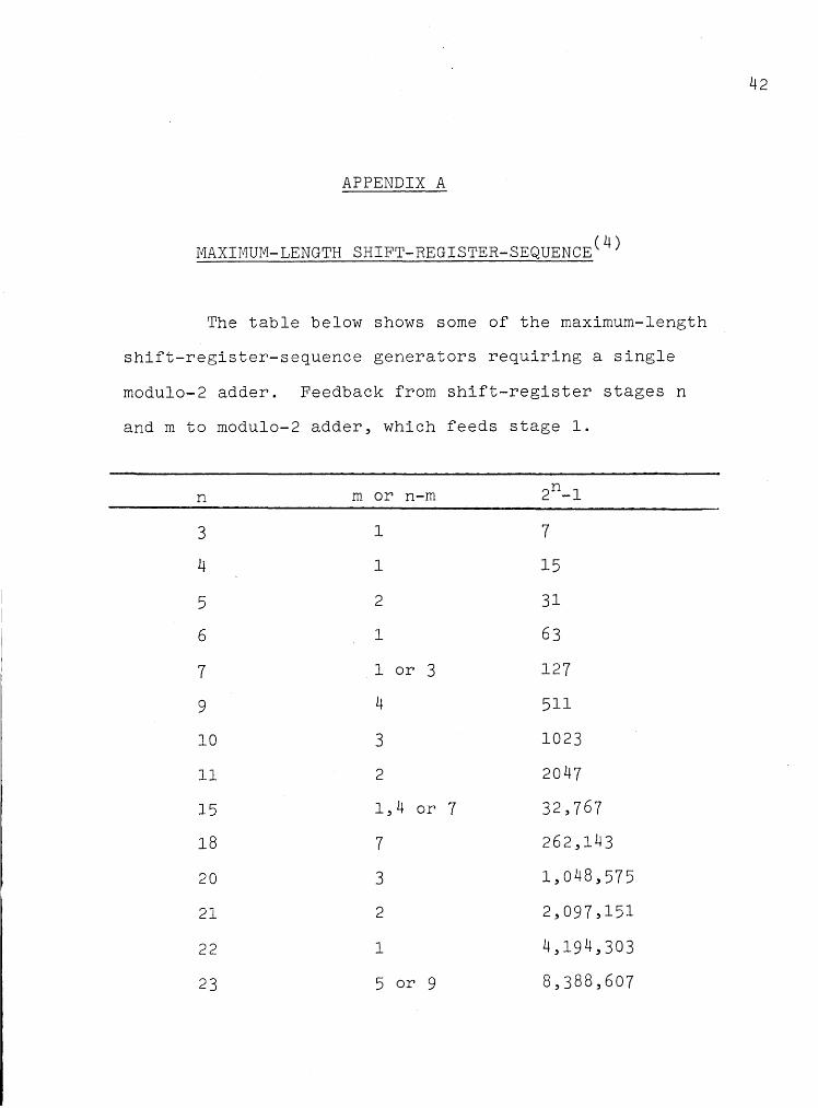
MAXIMUM-LENGTH SHIFT-REGISTER-SEQUENCE( 4)

The table below shows some of the maximum-length

shift-register-sequence generators requiring a single

modulo-2 adder. Feedback from shift-register stages n

and m to modulo-2 adder, which feeds stage 1.

n m or n-m 2n-l

3 1 7

4 1 15

5 2 31

6 1 63

7 1 or 3 127

9 4 511

10 3 1023

11 2 2047

15 1,4 or 7 32,767

18 7 262,143

20 3 1,048,575

21 2 2,097,151

22 1 4,194,303

23 5 or 9 8,388,607

42

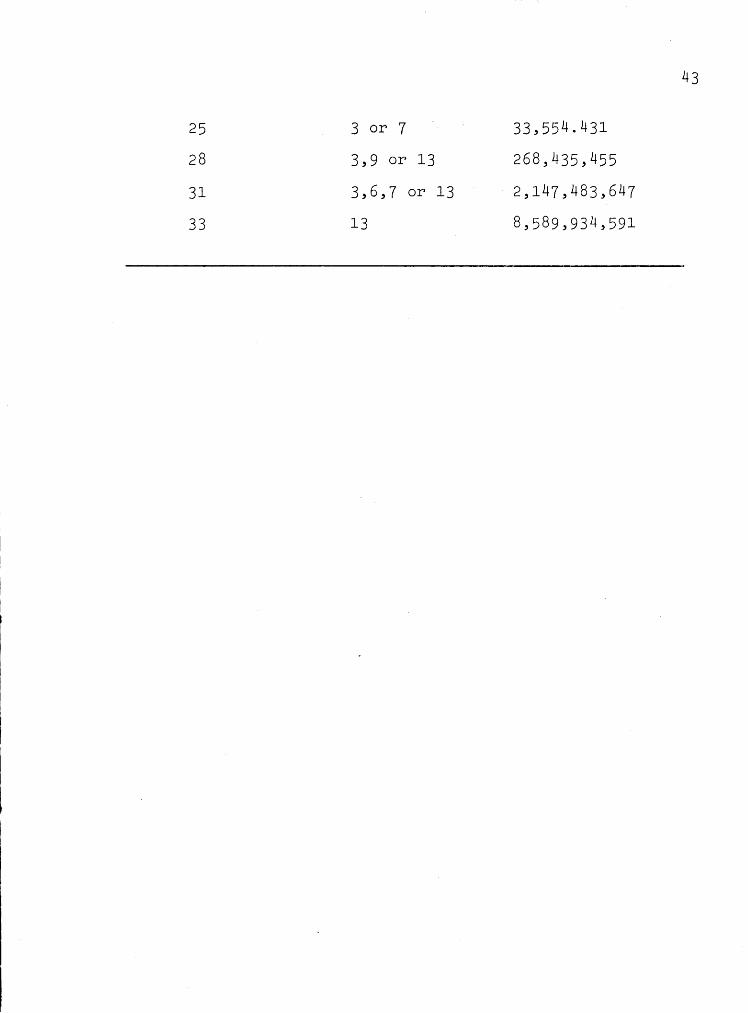
25

28

31

33

3 or 7

3,9 or 13

3,6,7 or 13

13

33,554.431

268,435,455

2,147,483,647

8,589,934,591

43

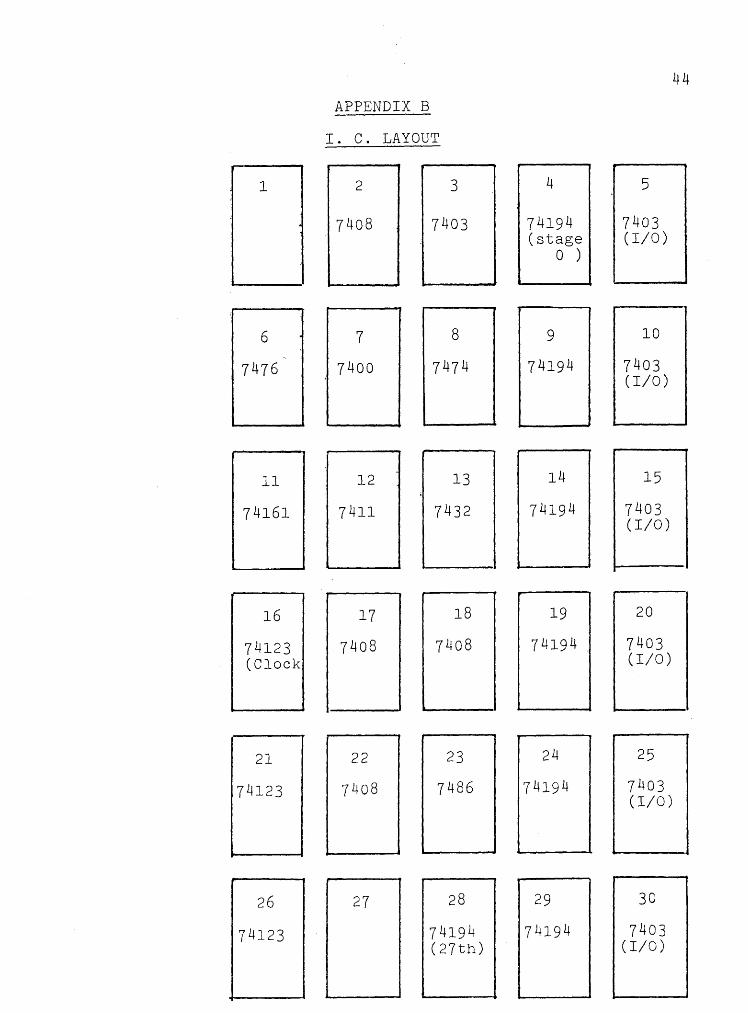
1

:1 I

6 .

7476

21

74123

26

74123

APPENDIX B

I. C. LAYOUT

2

7408

7

7400

22

7408

27

3

7403

8

7474

23

7486

28

74194 (27th)

4

74194 (stage

0 )

9

74194

24

74194

29

74194

5

7403 (I/O)

10

7403 (I/O)

25

7403 (I/O)

30

7403 (I/O)

44

REFERENCES

1. Hartley,M.G., "Digital Simulation Method",

IEE Monograph Series 15, Peter Peregrinus(l975).

2. Golumb,S.W., "Shift Register Sequences",

Holden-Day(l967).

3. Brandt,S., "Statistical and Computational Methods in

Data Analysis", North-Holland(l970).

4. Korn,G.A., "Random-Process Simulation and Measurement",

McGraw Hill(l966).

5. Data General Corporation, "Introduction to Programming

the Nova", 1972.

6. Data Gen. Corp., "User's Manual, Fortran 4", 1975.

7. Data Gen. Corp., "Extended Basic, User's Manual",1975.

45