Embed Size (px)
Citation preview

PSEG Site ESP Application
Part 3, Environmental Report
Rev. 4 2-i
CHAPTER 2
ENVIRONMENTAL DESCRIPTION
TABLE OF CONTENTS
Section Title Page
2.1 SITE LOCATION .......................................................................................... 2.1-1
2.1.1 DESCRIPTION OF THE EXISTING PSEG GENERATING STATIONS ......... 2.1-1 2.1.2 SITE LOCATION AND GENERAL SETTING ................................................. 2.1-2 2.1.3 REFERENCES ............................................................................................. 2.1-3
2.2 LAND ............................................................................................................ 2.2-1
2.2.1 THE SITE AND VICINITY ............................................................................. 2.2-1 2.2.1.1 The Site ............................................................................................. 2.2-1 2.2.1.2 The Vicinity ........................................................................................ 2.2-2 2.2.2 REGION ....................................................................................................... 2.2-4 2.2.3 TRANSMISSION LINE AND OFF-SITE AREAS ............................................ 2.2-5 2.2.3.1 Existing Transmission Corridors ......................................................... 2.2-5 2.2.3.2 Existing Access Road ......................................................................... 2.2-6 2.2.3.3 Proposed Transmission Macro-Corridors ........................................... 2.2-6 2.2.3.4 Proposed Access Road ...................................................................... 2.2-7 2.2.3.5 Other Proposed Off-Site Areas ........................................................... 2.2-8 2.2.4 REFERENCES ............................................................................................. 2.2-8
2.3 WATER ........................................................................................................ 2.3-1
2.3.1 HYDROLOGY ............................................................................................... 2.3-1 2.3.1.1 Surface Water Resources .................................................................. 2.3-1 2.3.1.1.1 Watershed Description ....................................................................... 2.3-1 2.3.1.1.1.1 Climate .............................................................................................. 2.3-2 2.3.1.1.1.2 Dams and Reservoirs ......................................................................... 2.3-3 2.3.1.1.2 Local Drainage ................................................................................... 2.3-4 2.3.1.1.3 Delaware River Flow .......................................................................... 2.3-5 2.3.1.1.3.1 Flow Duration Analysis ....................................................................... 2.3-5 2.3.1.1.3.2 Mass Curve Analysis .......................................................................... 2.3-6 2.3.1.1.3.3 Low Flow Analysis .............................................................................. 2.3-7 2.3.1.1.4 Historic Flooding and Annual Peak Flood Frequencies ...................... 2.3-8 2.3.1.1.5 Delaware Estuary ............................................................................... 2.3-8 2.3.1.1.5.1 Delaware Estuary Circulation and Freshwater Flow ........................... 2.3-10 2.3.1.1.5.1.1 Estuarine Dynamics ........................................................................... 2.3-10 2.3.1.1.5.1.2 Components of Estuarine Dynamics .................................................. 2.3-11 2.3.1.2 Groundwater Resources .................................................................... 2.3-18 2.3.1.2.1 Regional Hydrogeology ...................................................................... 2.3-18 2.3.1.2.2 Local Hydrogeology ........................................................................... 2.3-20 2.3.1.2.2.1 Fill Deposits ....................................................................................... 2.3-20

PSEG Site ESP Application
Part 3, Environmental Report
TABLE OF CONTENTS (CONTINUED)
Section Title Page
Rev. 4 2-ii
2.3.1.2.2.2 Alluvium ............................................................................................. 2.3-21 2.3.1.2.2.3 Kirkwood Formation ........................................................................... 2.3-21 2.3.1.2.2.4 Vincentown Formation ....................................................................... 2.3-23 2.3.1.2.2.5 Hornerstown Formation ...................................................................... 2.3-23 2.3.1.2.2.6 Navesink Formation ........................................................................... 2.3-24 2.3.1.2.2.7 Mount Laurel Formation ..................................................................... 2.3-25 2.3.1.2.2.8 Wenonah Formation ........................................................................... 2.3-25 2.3.1.2.2.9 Marshalltown Formation ..................................................................... 2.3-26 2.3.1.2.2.10 Englishtown Formation ....................................................................... 2.3-26 2.3.1.2.2.11 Woodbury Formation .......................................................................... 2.3-27 2.3.1.2.2.12 Merchantville Formation ..................................................................... 2.3-27 2.3.1.2.2.13 Potomac-Raritan-Magothy Units ........................................................ 2.3-27 2.3.1.2.3 Observation Well Data ....................................................................... 2.3-28 2.3.1.2.3.1 Alluvium ............................................................................................. 2.3-29 2.3.1.2.3.2 Vincentown Formation ....................................................................... 2.3-30 2.3.1.2.3.3 Hydrogeologic Properties ................................................................... 2.3-31 2.3.1.2.4 Hydraulic Communication Between Groundwater and Surface Water
Bodies ................................................................................................ 2.3-33 2.3.1.2.5 Summary ........................................................................................... 2.3-34 2.3.1.3 Transmission Corridors ...................................................................... 2.3-34 2.3.2 WATER USE ................................................................................................. 2.3-35 2.3.2.1 Regional Surface Water Use .............................................................. 2.3-37 2.3.2.1.1 Surface Water Use in the Vicinity ....................................................... 2.3-38 2.3.2.1.2 Surface Water Use at the PSEG Site ................................................. 2.3-38 2.3.2.2 Regional Groundwater Use ................................................................ 2.3-39 2.3.2.2.1 Groundwater Use in the Vicinity ......................................................... 2.3-40 2.3.2.2.1.1 Salem County, New Jersey ................................................................ 2.3-40 2.3.2.2.1.2 Cumberland County, New Jersey ....................................................... 2.3-40 2.3.2.2.1.3 Gloucester County, New Jersey ......................................................... 2.3-41 2.3.2.2.1.4 New Castle County, Delaware ............................................................ 2.3-41 2.3.2.2.2 Groundwater Use at the PSEG Site ................................................... 2.3-41 2.3.3 WATER QUALITY ......................................................................................... 2.3-43 2.3.3.1 Surface Water .................................................................................... 2.3-43 2.3.3.2 Groundwater ...................................................................................... 2.3-46 2.3.3.2.1 Regional Groundwater Quality ........................................................... 2.3-46 2.3.3.2.2 Local Groundwater Quality ................................................................. 2.3-46 2.3.4 REFERENCES ............................................................................................. 2.3-49
2.4 ECOLOGY .................................................................................................... 2.4-1
2.4.1 TERRESTRIAL ECOLOGY ........................................................................... 2.4-1 2.4.1.1 Terrestrial Habitats ............................................................................. 2.4-2 2.4.1.1.1 On-Site and Near Off-Site Habitats .................................................... 2.4-3 2.4.1.1.1.1 Wetlands and Aquatic Habitat ............................................................ 2.4-3 2.4.1.1.1.2 Old Field Habitat ................................................................................ 2.4-3
PSEG Site ESP Application
Part 3, Environmental Report
TABLE OF CONTENTS (CONTINUED)
Section Title Page
Rev. 4 2-iii
2.4.1.1.1.3 Developed Land Uses ........................................................................ 2.4-4 2.4.1.1.1.4 Agricultural Land ................................................................................ 2.4-4 2.4.1.1.2 Six-Mile Vicinity Habitat ...................................................................... 2.4-4 2.4.1.2 Wildlife ............................................................................................... 2.4-5 2.4.1.2.1 Birds .................................................................................................. 2.4-5 2.4.1.2.2 Mammals ........................................................................................... 2.4-7 2.4.1.2.3 Herpetofauna ..................................................................................... 2.4-7 2.4.1.3 Important Terrestrial Species and Habitats ......................................... 2.4-8 2.4.1.3.1 Birds .................................................................................................. 2.4-9 2.4.1.3.1.1 Cooper’s Hawk................................................................................... 2.4-9 2.4.1.3.1.2 Red-Shouldered Hawk ....................................................................... 2.4-10 2.4.1.3.1.3 Northern Harrier ................................................................................. 2.4-10 2.4.1.3.1.4 Bald Eagle ......................................................................................... 2.4-11 2.4.1.3.1.5 Osprey ............................................................................................... 2.4-12 2.4.1.3.1.6 Red-Headed Woodpecker .................................................................. 2.4-12 2.4.1.3.1.7 Northern Pintail .................................................................................. 2.4-13 2.4.1.3.1.8 Green-Winged Teal ............................................................................ 2.4-14 2.4.1.3.1.9 Mallard ............................................................................................... 2.4-14 2.4.1.3.1.10 American Black Duck ......................................................................... 2.4-15 2.4.1.3.1.11 Ring-Necked Duck ............................................................................. 2.4-15 2.4.1.3.1.12 Greater Scaup .................................................................................... 2.4-16 2.4.1.3.1.13 Bufflehead .......................................................................................... 2.4-16 2.4.1.3.1.14 American Coot ................................................................................... 2.4-17 2.4.1.3.1.15 Canada Goose ................................................................................... 2.4-18 2.4.1.3.1.16 Snow Goose ...................................................................................... 2.4-18 2.4.1.3.1.17 Hooded Merganser ............................................................................ 2.4-19 2.4.1.3.1.18 Common Merganser .......................................................................... 2.4-19 2.4.1.3.1.19 Red-Breasted Merganser ................................................................... 2.4-20 2.4.1.3.1.20 Wild Turkey ........................................................................................ 2.4-21 2.4.1.3.2 Mammals ........................................................................................... 2.4-21 2.4.1.3.2.1 River Otter ......................................................................................... 2.4-21 2.4.1.3.2.2 Muskrat .............................................................................................. 2.4-22 2.4.1.3.2.3 White-Tailed Deer .............................................................................. 2.4-23 2.4.1.3.3 Plant Communities ............................................................................. 2.4-23 2.4.1.3.4 Important Habitats – Wetlands ........................................................... 2.4-24 2.4.1.4 Disease Vectors and Pest Species ..................................................... 2.4-25 2.4.1.5 Wildlife Travel Corridors ..................................................................... 2.4-26 2.4.1.6 Existing Ecological Effects and Environmental Stresses .................... 2.4-26 2.4.1.7 Ongoing Ecological Studies ............................................................... 2.4-27 2.4.1.8 Off-Site Transmission and Access Corridors ...................................... 2.4-27 2.4.1.8.1 Off-Site Transmission ......................................................................... 2.4-27 2.4.1.8.2 Access Corridor ................................................................................. 2.4-28 2.4.2 AQUATIC ECOLOGY ................................................................................... 2.4-29 2.4.2.1 Aquatic Habitats ................................................................................. 2.4-29 2.4.2.1.1 Creeks and Ponds On or Near the PSEG Site ................................... 2.4-29
PSEG Site ESP Application
Part 3, Environmental Report
TABLE OF CONTENTS (CONTINUED)
Section Title Page
Rev. 4 2-iv
2.4.2.1.2 Delaware River .................................................................................. 2.4-30 2.4.2.1.2.1 Fish .................................................................................................... 2.4-30 2.4.2.1.2.2 Macroinvertebrates ............................................................................ 2.4-32 2.4.2.2 Important Aquatic Species .................................................................. 2.4-33 2.4.2.2.1 Threatened/Endangered Species and Candidates for Listing ............. 2.4-33 2.4.2.2.1.1 Shortnose Sturgeon ........................................................................... 2.4-34 2.4.2.2.1.2 Atlantic Sturgeon ................................................................................ 2.4-35 2.4.2.2.1.3 Loggerhead Turtle .............................................................................. 2.4-36 2.4.2.2.1.4 Atlantic Green Turtle .......................................................................... 2.4-37 2.4.2.2.1.5 Leatherback Turtle ............................................................................. 2.4-37 2.4.2.2.1.6 Hawksbill Turtle .................................................................................. 2.4-38 2.4.2.2.1.7 Kemp’s Ridley Turtle .......................................................................... 2.4-39 2.4.2.2.2 Commercial and Recreational Species ............................................... 2.4-39 2.4.2.2.2.1 Blueback Herring ............................................................................... 2.4-39 2.4.2.2.2.2 Alewife ............................................................................................... 2.4-40 2.4.2.2.2.3 American Shad .................................................................................. 2.4-41 2.4.2.2.2.4 Bay Anchovy ...................................................................................... 2.4-41 2.4.2.2.2.5 American Eel ..................................................................................... 2.4-42 2.4.2.2.2.6 Atlantic Menhaden ............................................................................. 2.4-42 2.4.2.2.2.7 Black Sea Bass .................................................................................. 2.4-43 2.4.2.2.2.8 Conger Eel ......................................................................................... 2.4-44 2.4.2.2.2.9 Weakfish ............................................................................................ 2.4-44 2.4.2.2.2.10 Channel Catfish ................................................................................. 2.4-45 2.4.2.2.2.11 Spot ................................................................................................... 2.4-46 2.4.2.2.2.12 Atlantic Silverside ............................................................................... 2.4-46 2.4.2.2.2.13 Northern Kingfish ............................................................................... 2.4-47 2.4.2.2.2.14 Silver Hake ........................................................................................ 2.4-47 2.4.2.2.2.15 Atlantic Croaker ................................................................................. 2.4-48 2.4.2.2.2.16 White Perch ....................................................................................... 2.4-48 2.4.2.2.2.17 Striped Bass ....................................................................................... 2.4-49 2.4.2.2.2.18 Summer Flounder .............................................................................. 2.4-50 2.4.2.2.2.19 Butterfish............................................................................................ 2.4-50 2.4.2.2.2.20 Black Drum ........................................................................................ 2.4-51 2.4.2.2.2.21 Bluefish .............................................................................................. 2.4-51 2.4.2.2.2.22 Northern Sea Robin ........................................................................... 2.4-52 2.4.2.2.2.23 Winter Flounder ................................................................................. 2.4-53 2.4.2.2.2.24 Windowpane Flounder ....................................................................... 2.4-54 2.4.2.2.2.25 Scup .................................................................................................. 2.4-54 2.4.2.2.3 Harvested Invertebrates ..................................................................... 2.4-55 2.4.2.2.3.1 Blue Crab ........................................................................................... 2.4-55 2.4.2.2.3.2 Eastern Oyster ................................................................................... 2.4-56 2.4.2.2.3.3 Horseshoe Crab ................................................................................. 2.4-57 2.4.2.2.3.4 Northern Quahog Clam ...................................................................... 2.4-57 2.4.2.2.4 Other Important Resources ................................................................ 2.4-58 2.4.2.2.4.1 Submerged Aquatic Vegetation .......................................................... 2.4-58
PSEG Site ESP Application
Part 3, Environmental Report
TABLE OF CONTENTS (CONTINUED)
Section Title Page
Rev. 4 2-v
2.4.2.2.4.2 Plankton (Phytoplankton and Zooplankton) ........................................ 2.4-58 2.4.2.2.5 Nuisance Species ............................................................................... 2.4-59 2.4.2.3 Habitat Importance and Essential Fish Habitat ................................... 2.4-59 2.4.2.3.1 Habitat Importance ............................................................................. 2.4-59 2.4.2.3.2 Essential Fish Habitat ......................................................................... 2.4-60 2.4.2.3.2.1 Butterfish ............................................................................................ 2.4-60 2.4.2.3.2.2 Windowpane Flounder ........................................................................ 2.4-61 2.4.2.3.2.3 Winter Flounder .................................................................................. 2.4-61 2.4.2.3.2.4 Summer Flounder ............................................................................... 2.4-61 2.4.2.4 Preexisting Environmental Stresses ................................................... 2.4-62 2.4.2.5 Off-Site Transmission Corridors .......................................................... 2.4-62 2.4.2.6 Access Corridor .................................................................................. 2.4-63 2.4.3 REFERENCES ............................................................................................. 2.4-63
2.5 SOCIOECONOMICS .................................................................................... 2.5-1
2.5.1 DEMOGRAPHY ............................................................................................ 2.5-1 2.5.1.1 Current and Projected Population Levels ........................................... 2.5-3 2.5.1.1.1 Resident Population Distribution within 0 to 10 Miles .......................... 2.5-3 2.5.1.1.2 Transient Population Distribution within 0 to 10 Miles ......................... 2.5-3 2.5.1.1.3 Resident Population Distribution within 10 to 50 Miles ........................ 2.5-4 2.5.1.1.4 Complete Distribution and Projection of the Resident Population ....... 2.5-5 2.5.1.2 Population Data by Political Jurisdiction ............................................. 2.5-5 2.5.1.2.1 Characteristics of the Resident Population ......................................... 2.5-6 2.5.1.2.1.1 New Jersey ........................................................................................ 2.5-6 2.5.1.2.1.2 Delaware ............................................................................................ 2.5-8 2.5.1.3 Low Population Zone .......................................................................... 2.5-9 2.5.1.4 Special Facilities and Population Centers ........................................... 2.5-9 2.5.1.4.1 Special Facilities ................................................................................. 2.5-9 2.5.1.4.2 Population Centers ............................................................................. 2.5-10 2.5.1.5 Population Density for Socioeconomic Analyses ................................ 2.5-11 2.5.1.6 Exclusion Area Boundary ................................................................... 2.5-11 2.5.2 COMMUNITY CHARACTERISTICS ............................................................. 2.5-12 2.5.2.1 Economic Base .................................................................................. 2.5-13 2.5.2.1.1 Regional Economic Base (50-Mile Radius) ......................................... 2.5-13 2.5.2.1.1.1 Major Industries and Associated Employment Levels ......................... 2.5-13 2.5.2.1.1.2 Heavy Construction Industries and Construction Trade Workforce ..... 2.5-14 2.5.2.1.1.3 Labor Force and Employment Trends ................................................. 2.5-14 2.5.2.1.1.4 Characterization of Construction Workforce ....................................... 2.5-16 2.5.2.1.2 Economic Base within the Four-County Region of Influence .............. 2.5-16 2.5.2.1.2.1 Major Industries and Associated Employment Levels ......................... 2.5-16 2.5.2.1.2.1.1 Heavy Construction Industries and Construction Trade Workforce ..... 2.5-17 2.5.2.1.2.1.2 Labor Force and Employment Trends ................................................. 2.5-17 2.5.2.2 Political Tax and Regional Planning Authorities ................................. 2.5-19 2.5.2.2.1 Political Tax Jurisdictions .................................................................... 2.5-19

PSEG Site ESP Application
Part 3, Environmental Report
TABLE OF CONTENTS (CONTINUED)
Section Title Page
Rev. 4 2-vi
2.5.2.2.1.1 Delaware Taxes .................................................................................. 2.5-20 2.5.2.2.1.2 New Jersey ........................................................................................ 2.5-20 2.5.2.2.1.3 Pennsylvania ...................................................................................... 2.5-20 2.5.2.2.2 Regional Planning Authorities ............................................................. 2.5-21 2.5.2.3 Personal Income and Housing ............................................................ 2.5-22 2.5.2.3.1 Personal Income within the 50-Mile Region ........................................ 2.5-22 2.5.2.3.2 Personal Income within the Four-County Region of Influence............. 2.5-22 2.5.2.4 Housing .............................................................................................. 2.5-23 2.5.2.4.1 Housing within the 50-Mile Region ..................................................... 2.5-23 2.5.2.4.2 Housing within the Four-County Region of Influence .......................... 2.5-23 2.5.2.5 Education System .............................................................................. 2.5-24 2.5.2.5.1 Schools within the 50-Mile Radius ...................................................... 2.5-24 2.5.2.5.1.1 Public Schools .................................................................................... 2.5-24 2.5.2.5.1.2 Colleges and Universities ................................................................... 2.5-25 2.5.2.5.2 Schools within the Four-County Region of Influence .......................... 2.5-25 2.5.2.5.2.1 Public Schools .................................................................................... 2.5-25 2.5.2.5.2.2 Colleges ............................................................................................. 2.5-26 2.5.2.6 Aesthetics and Recreation (50-Mile Region) ....................................... 2.5-26 2.5.2.6.1 Visual Resources ............................................................................... 2.5-26 2.5.2.6.2 Recreation .......................................................................................... 2.5-27 2.5.2.7 Tax Structure and Distribution of Present Revenues ........................... 2.5-28 2.5.2.7.1 Delaware ............................................................................................ 2.5-28 2.5.2.7.2 New Jersey ........................................................................................ 2.5-29 2.5.2.7.3 Pennsylvania ...................................................................................... 2.5-29 2.5.2.8 Land Use ............................................................................................ 2.5-29 2.5.2.8.1 New Castle County ............................................................................. 2.5-30 2.5.2.8.2 Salem County ..................................................................................... 2.5-31 2.5.2.8.3 Cumberland County ............................................................................ 2.5-32 2.5.2.8.4 Gloucester County .............................................................................. 2.5-34 2.5.2.9 Community Infrastructure and Public Services ................................... 2.5-35 2.5.2.9.1 Public Water Supplies and Water Treatment Systems ........................ 2.5-35 2.5.2.9.1.1 Salem County ..................................................................................... 2.5-35 2.5.2.9.1.2 Cumberland County ............................................................................ 2.5-36 2.5.2.9.1.3 Gloucester County .............................................................................. 2.5-36 2.5.2.9.1.4 New Castle County ............................................................................. 2.5-37 2.5.2.9.2 Police, Fire, and Medical Services ...................................................... 2.5-37 2.5.2.9.2.1 Police Protection ................................................................................ 2.5-37 2.5.2.9.2.2 Firefighting and Emergency Medical Services .................................... 2.5-38 2.5.2.9.2.3 Medical Services ................................................................................ 2.5-38 2.5.2.9.2.4 Social Services and Major Community Structures .............................. 2.5-39 2.5.2.9.3 Emergency Planning .......................................................................... 2.5-40 2.5.2.10 Transportation .................................................................................... 2.5-41 2.5.2.10.1 Roads ................................................................................................. 2.5-42 2.5.2.10.2 Road and Highway Mileage within the Region and Region of
Influence ............................................................................................ 2.5-42

PSEG Site ESP Application
Part 3, Environmental Report
TABLE OF CONTENTS (CONTINUED)
Section Title Page
Rev. 4 2-vii
2.5.2.10.2.1 Traffic Conditions ............................................................................... 2.5-43 2.5.2.10.2.2 Atlantic Coast Hurricane Evacuation Routes ...................................... 2.5-43 2.5.2.10.3 Rail .................................................................................................... 2.5-43 2.5.2.10.4 Waterways ......................................................................................... 2.5-43 2.5.2.10.5 Airports .............................................................................................. 2.5-44 2.5.3 HISTORIC PROPERTIES .................................................................. 2.5-44 2.5.3.1 Prehistoric Background ...................................................................... 2.5-44 2.5.3.2 Historic Background ........................................................................... 2.5-45 2.5.3.3 Archaeological Sites within or Near the PSEG Site ............................ 2.5-45 2.5.3.3.1 Upland Archaeology ........................................................................... 2.5-45 2.5.3.3.2 Underwater Archaeology .................................................................... 2.5-46 2.5.3.3.3 Buried Prehistoric Soils at the PSEG Site .......................................... 2.5-46 2.5.3.4 Historic Structures and Districts Identified within the Vicinity of the
PSEG Site .......................................................................................... 2.5-47 2.5.3.5 Potentially Eligible Structures and Districts in Near Off-Site Areas. .... 2.5-47 2.5.3.6 Native American and State Agency Consultation ................................ 2.5-48 2.5.3.7 Transmission Corridors ...................................................................... 2.5-48 2.5.4 ENVIRONMENTAL JUSTICE ........................................................................ 2.5-49 2.5.4.1 Methodology ...................................................................................... 2.5-49 2.5.4.2 Minority Populations ........................................................................... 2.5-49 2.5.4.3 Low-Income Populations .................................................................... 2.5-50 2.5.4.4 Distribution of Minority and Low-Income Populations ......................... 2.5-51 2.5.4.5 Minority and Low-Income Population Trends ...................................... 2.5-52 2.5.4.6 Migrant Populations ........................................................................... 2.5-53 2.5.5 NOISE .......................................................................................................... 2.5-54 2.5.6 REFERENCES ............................................................................................. 2.5-55
2.6 GEOLOGY ................................................................................................... 2.6-1
2.6.1 GEOLOGIC SETTING .................................................................................. 2.6-1 2.6.2 PSEG SITE STRATIGRAPHY ...................................................................... 2.6-1 2.6.2.1.1 PSEG Site Stratigraphic Units and Geologic Formations .................... 2.6-2 2.6.2.1.2 Description of PSEG Site Stratigraphic Units and Geologic
Formations ......................................................................................... 2.6-3 2.6.2.1.2.1 Cretaceous Strata .............................................................................. 2.6-3 2.6.2.1.2.1.1 Potomac Formation ............................................................................ 2.6-3 2.6.2.1.2.1.2 Magothy Formation ............................................................................ 2.6-3 2.6.2.1.2.1.3 Merchantville Formation ..................................................................... 2.6-4 2.6.2.1.2.1.4 Woodbury Formation .......................................................................... 2.6-4 2.6.2.1.2.1.5 Englishtown Formation ....................................................................... 2.6-4 2.6.2.1.2.1.6 Marshalltown Formation ..................................................................... 2.6-5 2.6.2.1.2.1.7 Wenonah Formation ........................................................................... 2.6-5 2.6.2.1.2.1.8 Mount Laurel Formation ..................................................................... 2.6-5 2.6.2.1.2.1.9 Navesink Formation ........................................................................... 2.6-6 2.6.2.1.2.2 Paleogene Strata (Lower Tertiary) ...................................................... 2.6-6

PSEG Site ESP Application
Part 3, Environmental Report
TABLE OF CONTENTS (CONTINUED)
Section Title Page
Rev. 4 2-viii
2.6.2.1.2.2.1 Hornerstown Formation ...................................................................... 2.6-6 2.6.2.1.2.2.2 Vincentown Formation ....................................................................... 2.6-7 2.6.2.1.2.3 Neogene Strata (Upper Tertiary) ......................................................... 2.6-7 2.6.2.1.2.3.1 Kirkwood Formation ........................................................................... 2.6-7 2.6.2.1.2.4 Quaternary Strata ............................................................................... 2.6-8 2.6.3 REFERENCES ............................................................................................. 2.6-9
2.7 METEOROLOGY AND AIR QUALITY .......................................................... 2.7-1
2.7.1 REGIONAL CLIMATOLOGY ......................................................................... 2.7-1 2.7.1.1 Data Sources ..................................................................................... 2.7-1 2.7.1.2 General Climate Description .............................................................. 2.7-2 2.7.1.3 Normal, Mean, and Extreme Regional Climatological Conditions ....... 2.7-2 2.7.1.3.1 Temperature ....................................................................................... 2.7-2 2.7.1.3.2 Atmospheric Water Vapor .................................................................. 2.7-2 2.7.1.3.3 Precipitation ....................................................................................... 2.7-3 2.7.1.3.4 Wind Conditions ................................................................................. 2.7-3 2.7.2 REGIONAL AIR QUALITY ............................................................................ 2.7-3 2.7.2.1 Background Air Quality ....................................................................... 2.7-3 2.7.2.2 Projected Air Quality .......................................................................... 2.7-3 2.7.2.3 Restrictive Dispersion Conditions ....................................................... 2.7-4 2.7.3 SEVERE WEATHER ..................................................................................... 2.7-4 2.7.3.1 Thunderstorms and Lightning ............................................................. 2.7-4 2.7.3.2 Extreme Winds ................................................................................... 2.7-4 2.7.3.3 Tornadoes .......................................................................................... 2.7-5 2.7.3.4 Hail, Snowstorms, and Ice Storms...................................................... 2.7-5 2.7.3.5 Tropical Cyclones ............................................................................... 2.7-6 2.7.4 LOCAL METEOROLOGY ............................................................................. 2.7-6 2.7.4.1 Normal, Mean, and Extreme Values ................................................... 2.7-6 2.7.4.1.1 Temperature ....................................................................................... 2.7-6 2.7.4.1.2 Atmospheric Moisture Content ........................................................... 2.7-6 2.7.4.1.3 Precipitation ....................................................................................... 2.7-7 2.7.4.1.4 Fog .................................................................................................... 2.7-7 2.7.4.2 Average Wind Direction and Wind Speed Conditions ......................... 2.7-7 2.7.4.3 Wind Direction Persistence ................................................................ 2.7-8 2.7.4.4 Atmospheric Stability .......................................................................... 2.7-8 2.7.4.5 Topographic Description and Potential Modifications ......................... 2.7-8 2.7.5 REFERENCES ............................................................................................. 2.7-9
2.8 RELATED FEDERAL AND OTHER PROJECT ACTIVITIES ......................... 2.8-1
2.8.1 FEDERAL PROJECT ACTIVITIES ................................................................ 2.8-1 2.8.1.1 USACE Delaware River Channel Deepening ..................................... 2.8-1 2.8.1.2 Use of USACE Lands ......................................................................... 2.8-2 2.8.2 NON-FEDERAL PROJECT ACTIVITIES ....................................................... 2.8-3

PSEG Site ESP Application
Part 3, Environmental Report
TABLE OF CONTENTS (CONTINUED)
Section Title Page
Rev. 4 2-ix
2.8.2.1 Mid-Atlantic Power Pathway (MAPP) ................................................. 2.8-3 2.8.2.2 Liquified Natural Gas Facilities ........................................................... 2.8-4 2.8.2.3 Southern New Jersey to Philadelphia Mass Transit and Philadelphia
Waterfront Transit Expansions ........................................................... 2.8-4 2.8.2.4 New Jersey and Philadelphia Ports Improvements ............................. 2.8-5 2.8.2.5 Mad Horse Creek Wildlife Management Area Habitat Restoration ...... 2.8-5 2.8.3 REFERENCES ............................................................................................. 2.8-6
PSEG Site ESP Application
Part 3, Environmental Report
Rev. 4 2-x
LIST OF TABLES
Number Title
2.2-1 Land Use within the PSEG Plant Site Property Boundary and Construction Support Facilities
2.2-2 Land Use in the Vicinity (6-Mile Radius) and Region (50-Mile Radius) of the PSEG Site
2.2-3 Land Use in the Existing PSEG Transmission Line Corridors and Existing Access Road Rights-of-Way
2.2-4 Land Use/Land Cover (LULC) within Each Off-Site Transmission Macro-Corridor
2.2-5 Principal Agricultural Crops within the New Castle (DE), Cumberland (NJ), Gloucester (NJ), and Salem (NJ) Counties as of 2007
2.3-1 Delaware River Subbasins and Drainage Areas Above and Below the PSEG Site
2.3-2 Selected Point Precipitation Frequency Estimates
2.3-3 Inventory of Reservoirs in the Delaware River Basin
2.3-4 Tributary Streams in the Vicinity of the PSEG Site
2.3-5 Monthly and Annual Mean Daily Streamflow Statistics – Delaware River at Trenton, New Jersey (Period of Record February 1, 1913 through May 3, 2009)
2.3-6 Monthly Mean Streamflow Statistics – Delaware River at Trenton, New Jersey (Period of Record October 1912 through September 2008)
2.3-7 Flood Discharge Frequency – Alloway Creek
2.3-8 Summary of Selected Physical Features of the Delaware Estuary
2.3-9 Regional and Site-Specific Aquifer Characteristics
2.3-10 Summary of Public Water Supply Wells within a 25-Mile Radius of the PSEG Site
2.3-11 Summary of Groundwater Users within the 25-Mile Radius
2.3-12 Observation Well Installation Details
2.3-13 Groundwater Elevations, January to December 2009
2.3-14 Groundwater Elevation Data Range (in Feet NAVD 1988) for HCGS and SGS Groundwater Wells, 2000 – 2009
2.3-15 Summary of Horizontal Hydraulic Gradients
2.3-16 Summary of Vertical Hydraulic Gradients
2.3-17 Summary of Average Hydraulic Conductivities

PSEG Site ESP Application
Part 3, Environmental Report
LIST OF TABLES (CONTINUED)
Rev. 4 2-xi
Number Title
2.3-18 Summary of Tidal Study Results
2.3-19 Summary of Surface Water and Shallow Groundwater Elevations at Piezometers
2.3-20 Water Withdrawal Estimates by Source in Delaware River Basin – Lower Estuary and Bay Regions
2.3-21 Peak Month Withdrawal and Consumptive Uses by Sector for Dry Year (1995) and Wet Year (1996)
2.3-22 Delaware River Basin Water Supply Reservoirs
2.3-23 Water Withdrawals and Consumptive Use by Power Generation Facilities (1995 Average Demands)
2.3-24 HCGS and SGS Annual Groundwater Pumpage (2002 – 2009)
2.3-25 Summary of Analytical Data – Delaware Estuary Locations (AS-8)
2.3-26 Summary of Analytical Data – Artificial Pond Locations (AS-4, AS-9, AS-14)
2.3-27 Summary of Analytical Data – Marsh Locations (AS-1, AS- 2, AS- 3, AS-5, AS-6, AS-10, and AS-11)
2.3-28 Summary of Analytical Data for Upper (Alluvium) New Plant Observation Well Locations
2.3-29 Summary of Analytical Data for Upper (Alluvium) Eastern Observation Well Locations
2.3-30 Summary of Analytical Data for Lower (Vincentown) New Plant Observation Well Locations
2.3-31 Summary of Analytical Data for Lower (Vincentown) Eastern Observation Well Locations
2.4-1 Summary of Terrestrial Surveys Conducted within the PSEG Site and Vicinity, 2009 – 2010
2.4-2 Land Use/land Cover within the PSEG Site Property Boundary
2.4-3 Land Use/Land Cover within the 6-Mile Vicinity of the PSEG Site
2.4-4 Mammals Observed On-Site and in the Vicinity of the PSEG Site, 2009 – 2010
2.4-5 Reptiles and Amphibians Observed On-Site and in the Vicinity of the PSEG Site, 2009 - 2010
2.4-6 Birds Observed Seasonally On-Site and in the Vicinity of the PSEG Site, 2009 – 2010

PSEG Site ESP Application
Part 3, Environmental Report
LIST OF TABLES (CONTINUED)
Rev. 4 2-xii
Number Title
2.4-7 Recorded Endangered and Threatened Species Potentially Occurring in the Vicinity of the PSEG Site
2.4-8 Important Terrestrial Species Potentially Occurring within the Vicinity of the PSEG Site
2.4-9 Terrestrial Plants Observed Seasonally On-Site and in the Vicinity of the PSEG Site, 2009
2.4-10 Land Use/Land Cover (LULC) within Each Off-Site Transmission Macro-Corridor
2.4-11 National Wetland Inventory (NWI) Wetlands within the 5-Mile Wide Macro-Corridor Study Area
2.4-12 Species Composition and Abundance of Fish Collections from Ponds on the PSEG Site, By Season, 2009
2.4-13 Taxonomic Composition and Abundance in Macroinvertebrate Surveys Collected by Ponar Dredge in Ponds on the PSEG Site
2.4-14 Species Composition and Abundance of Fish Collections from Small Marsh Creeks on or near the PSEG Site, By Season, 2009
2.4-15 Taxonomic Composition and Abundance in Macroinvertebrate Surveys Collected by Ponar Dredge in Marsh Creeks on or near the PSEG Site, 2009
2.4-16 Species Composition and Abundance in Fish Surveys of Small (Sampled by Weir) and Large (Sampled by Trawling) Segments of Marsh Creek Systems in the Vicinity of the PSEG Site, 2003 – 2007
2.4-17 Species Composition and Density in Impingement Samples at SGS, 2003 – 2007
2.4-18 Comparison of Species Composition and Mean Density (#/106 m3) in Impingement and Entrainment Samples at SGS, 5-Year Mean (2003 – 2007) Versus 13-Year Mean (1995 – 2007)
2.4-19 Comparison of Species Composition and Density (#/106 m3) Between Impingement Samples at SGS (2003 – 2007) and Samples at HCGS (1986 – 1987)
2.4-20 Seasonal Patterns of Species Composition and Mean Density (#/106 m3) in Impingement Samples at SGS, 2003 – 2007
2.4-21 Species Composition and Abundance in Entrainment Samples from SGS, 2003 – 2007)
2.4-22 Seasonal Patterns of Species Composition and Mean Density (#/106 m3) in Entrainment Samples at SGS, 2003 – 2007
2.4-23 Species Composition and Abundance in Fish Surveys of the Delaware River

PSEG Site ESP Application
Part 3, Environmental Report
LIST OF TABLES (CONTINUED)
Rev. 4 2-xiii
Number Title
(River Miles 40 – 60) near the PSEG Site, 2003 – 2007
2.4-24 Macroinvertebrate Taxa Collected in Ponar Surveys from the Delaware River near Artificial Island, 1971 – 1976
2.4-25 Taxonomic Composition and Abundance in Macroinvertebrate Surveys Collected by Ponar Dredge in the Delaware River near the PSEG Site, 2009
2.4-26 Important Aquatic Species Potentially Occurring in the Vicinity of the PSEG Site
2.4-27 Commercial and Recreational Harvests of Important Species in NJ and DE (2007)
2.4-28 EFH for Relevant Federally Managed Species in the Vicinity of the PSEG Site
2.4-29 Stream Length within Each Potential Off-Site Transmission Macro-Corridor
2.5-1 HCGS and SGS Employee Distribution by State and County as of 2008
2.5-2 Counties (by State) within 10 Miles and 50 Miles of the PSEG Site
2.5-3 Resident Population Distribution within 0 to 10 Miles of the PSEG Site, 2000 to 2081
2.5-4 Populations and Growth Rates of Municipalities within 10 Miles of the PSEG Site
2.5-5 Transient Population Distribution within 10 Miles of the PSEG Site, 2008 to 2081
2.5-6 Transient Population Estimates within 10 Miles of the PSEG Site, 2008
2.5-7 Resident Population Distribution within 10 to 50 Miles of the PSEG Site, 2000 to 2081
2.5-8 Resident Population Distribution and Projections within 50 Miles of the PSEG Site
2.5-9 Population Statistics for Cumberland, Gloucester, Salem and New Castle Counties and Selected Communities within 10 Miles of the PSEG Site
2.5-10 Population Characteristics for Counties and Selected Communities within 10 Miles of the PSEG Site
2.5-11 Schools and Daycare Facilities within 10 Miles of the PSEG Site
2.5-12 Employment Locations within 10 Miles of the PSEG Site
2.5-13 Other Special Facilities within 10 Miles of the PSEG Site
2.5-14 Population Centers with Over 25,000 People within 50 Miles of the PSEG Site
2.5-15 Description of Sparseness and Proximity Demographic Categories

PSEG Site ESP Application
Part 3, Environmental Report
LIST OF TABLES (CONTINUED)
Rev. 4 2-xiv
Number Title
2.5-16 Generic Environmental Impact Statement Sparseness and Proximity Matrix
2.5-17 Operation-Related Payroll for HCGS and SGS (2005 to 2008) for States and Counties within 50 Miles of the PSEG Site
2.5-18 Top Employers for Counties within 50 Miles of the PSEG Site
2.5-19 Employment and Unemployment Trends in the 25 Counties within 50 Miles of the PSEG Site, 1995 to 2008
2.5-20 Projected Employment Levels for Relevant Construction Trades within 50 Miles of the PSEG Site
2.5-21 Employment by Industry within 50 Miles of the PSEG Site, 1990 to 2007
2.5-22 Peak Construction Trade Labor and On-Site Labor Estimates for a Two-Unit AP1000 Plant
2.5-23 Estimated Construction Workforce Requirements by Construction Month for a Two-Unit AP1000 Plant
2.5-24 Top 10 Employers in Four-County Region of Influence of the PSEG Site
2.5-25 Employment Trends in the Four-County PSEG Site Region of Influence, 1995 to 2008
2.5-26 Projected 2016 Employment Levels for Relevant Construction Trades for PSEG Site Region of Influence
2.5-27 Employment by Industry for the Four-County Region of Influence for the PSEG Site, 1990 to 2007
2.5-28 Salem and Hope Creek Operation-related Purchases for Materials and Services from 2005 to 2008 with PSEG Site Region
2.5-29 Corporate, Income, Property, and Sales Tax Rates for 2008 for States and Region of Influence Counties within a 50-Mile Radius of the PSEG Site
2.5-30 Personal Income for 25 Counties within 50 Miles of the PSEG Site and Four-County Region of Influence, 1990 to 2007
2.5-31 Housing Information for Counties within 50 Miles of the PSEG Site, 1990 to 2007
2.5-32 Housing Information for Four-County Region of Influence of the PSEG Site, 1990 to 2007
2.5-33 School Enrollments and Capacities within 50 Miles of the PSEG Site, 2008

PSEG Site ESP Application
Part 3, Environmental Report
LIST OF TABLES (CONTINUED)
Rev. 4 2-xv
Number Title
2.5-34 School Enrollments and Capacities in the PSEG Site Four-County Region of Influence
2.5-35 Colleges and Universities within 50 Miles of the PSEG Site and Four-County Region of Influence
2.5-36 Refuges, Trusts and Parks within 50 Miles of PSEG Site
2.5-37 Taxes Paid by PSEG for the Hope Creek and Salem Generating Stations, and Energy and Environmental Resource Center
2.5-38 Major Water Suppliers (Serving 5000 or More People) within PSEG Site Region of Influence
2.5-39 Public Wastewater Treatment Systems in Four-County Region of Influence of PSEG Site
2.5-40 Police and Fire Personnel within 50 Miles of the PSEG Site and Four-County Region of Influence
2.5-41 Physicians and Hospital Beds within 50 Miles of the PSEG Site and Four-County Region of Influence
2.5-42 Road and Highway Mileage within 50 Miles of the PSEG Site and its Region of Influence
2.5-43 Annual Average Daily Traffic Counts on Roads in Proximity to the PSEG Site
2.5-44 International and General Aviation Airports within 50 Miles of the PSEG Site
2.5-45 Identified Historic Properties Located in the Proposed Causeway and Parking Areas
2.5-46 Historic Properties Listed on the National Register of Historic Places (NRHP) Located within a 10-Mi. Radius of the PSEG Site
2.5-47 Environmental Justice Populations within 50-Mile Radius of PSEG Site
2.5-48 Environmental Justice Populations for Selected Counties within 50-Mile Radius of PSEG Site
2.5-49 Population Trends in the 50-Mile Region
2.5-50 Population Trends in 10-County Delaware Valley Regional Planning Commission (DVRPC) Region
2.5-51 Farms that Employ Migrant Labor in the 50-Mile Region
2.5-52 Farms that Employ Migrant Labor for Selected Counties in New Jersey
2.5-53 Minority Farm Operators in the 50-Mile Region

PSEG Site ESP Application
Part 3, Environmental Report
LIST OF TABLES (CONTINUED)
Rev. 4 2-xvi
Number Title
2.5-54 Ambient Noise Levels at the HCGS and SGS in February 2009
2.7-1 Mean Seasonal and Annual Morning and Afternoon Mixing Heights and Wind Speeds at the PSEG Site

PSEG Site ESP Application
Part 3, Environmental Report
Rev. 4 2-xvii
LIST OF FIGURES
Number Title
2.1-1 Site Location
2.1-2 Site Location Vicinity (6-mile) and Region (50-mile)
2.1-3 View of PSEG Site
2.2-1 PSEG Site and Near Off-Site Land Use
2.2-2 Land Use within the Vicinity of the PSEG Site
2.2-3 Farmland Resources
2.2-4 Regional Land Use
2.2-5 Major Regional Transportation Features
2.2-6 Existing PSEG Transmission Corridors
2.3-1 Site Vicinity – Surface Water Resources
2.3-2 Delaware River Watershed
2.3-3 Daily Mean Flow Duration Curves – Delaware River at Trenton, NJ
2.3-4 Delaware River at Trenton, NJ – Cumulative Flow Volume and Departure from Long-Term Average
2.3-5 Delaware River at Trenton, NJ – Seasonal Distribution of Annual Minimum 7-Day Average Low Flow
2.3-6 FEMA 100-Year Floodplain – PSEG Site
2.3-7 Delaware Estuary Tidal Ranges along the Navigation Channel
2.3-8 Ebb and Flood Tide Current Velocity Duration Curves – Reedy Point
2.3-9 Hydrographic Transects of Salinity and Suspended-Sediment Concentration in the Delaware Estuary
2.3-10 Daily Mean Water Temperature Duration Curves – Reedy Island Jetty
2.3-11 Mean Daily Average Water Temperature at Reedy Island Jetty (USGS)
2.3-12 Contours of Measured Surface Temperatures for a Flood Phase on May 29, 1998
2.3-13 Contours of Modeled Surface Temperatures for Slack Phase (End of Flood Tide) on May 29, 1998
2.3-14 Monthly TSS Concentrations near PSEG Site
2.3-15 Surface Water and Sediment Grain-Size Sampling Locations
2.3-16 Grain Size Distribution – Estuary Sediments (0 – 6 Inches)
PSEG Site ESP Application
Part 3, Environmental Report
LIST OF FIGURES (CONTINUED)
Rev. 4 2-xviii
Number Title
2.3-17 Delaware River Bathymetric Map – RM 51 to RM 55
2.3-18 Hydrostratigraphic Classification for the PSEG Site
2.3-19 Hydrogeology, Extent of Major Aquifers or Aquifer Systems in NJ
2.3-20 NJ & DE Well Head Protection Areas and NJ Public Supply Wells Within 25 Miles of the PSEG Site
2.3-21 Surface and Groundwater Sampling Locations
2.3-22 Cross-Section Orientation
2.3-23 Cross-Section A-A’ Orientation
2.3-24 Cross-Section B-B’ Orientation
2.3-25 2009 Precipitation Data
2.3-26 Groundwater Elevations: New Plant Location
2.3-27 Groundwater Elevations: Eastern Location
2.3-28 Groundwater Elevations: Upper Wells in New Plant Location
2.3-29 Potentiometric Contour Map New Plant Location – Alluvium, February 2009
2.3-30 Potentiometric Contour Map New Plant Location – Alluvium, April 2009
2.3-31 Potentiometric Contour Map New Plant Location – Alluvium, July 2009
2.3-32 Potentiometric Contour Map New Plant Location – Alluvium, September 2009
2.3-33 Groundwater Elevations: Upper Wells in Eastern Location
2.3-34 Potentiometric Contour Map Eastern Location – Alluvium February 2009
2.3-35 Potentiometric Contour Map Eastern Location – Alluvium, April 2009
2.3-36 Potentiometric Contour Map Eastern Location – Alluvium, July 2009
2.3-37 Potentiometric Contour Map Eastern Location – Alluvium September 2009
2.3-38 Groundwater Elevations: Lower Wells in New Plant Location
2.3-39 Potentiometric Contour Map New Plant Location – Vincentown Formation, February 2009
2.3-40 Potentiometric Contour Map New Plant Location – Vincentown Formation, April 2009
2.3-41 Potentiometric Contour Map New Plant Location – Vincentown Formation, July 2009

PSEG Site ESP Application
Part 3, Environmental Report
LIST OF FIGURES (CONTINUED)
Rev. 4 2-xix
Number Title
2.3-42 Potentiometric Contour Map New Pant Location – Vincentown Formation, September 2009
2.3-43 Groundwater Elevations: Lower Wells in Eastern Location
2.3-44 Potentiometric Contour Map Eastern Location –Vincentown Formation, February 2009
2.3-45 Potentiometric Contour Map Eastern Location –Vincentown Formation, April 2009
2.3-46 Potentiometric Contour Map Eastern Location –Vincentown Formation, July 2009
2.3-47 Potentiometric Contour Map Eastern Location – Vincentown Formation, September 2009
2.3-48 Tidal Effects – Summary of Water Level Elevation vs. Time
2.3-49 Tidal Effects – Barge Slip Location and Observation Well NOW-1U
2.3-50 Tidal Effects – Barge Slip Location and Observation Well NOW-1L
2.3-51 Tidal Effects – Barge Slip Location and Observation Well NOW-3U
2.3-52 Tidal Effects – Barge Slip Location and Observation Well NOW-3L
2.3-53 Summary of Potentiometric Contours for River Bed Deposits, September 2009
2.4-1 Land Use/Land Cover within the PSEG Site
2.4-2 Land Use/Land Cover within the PSEG Site and Near Off-Site Areas
2.4-3 Land Use/Land Cover within the PSEG 6-Mi. Vicinity
2.4-4 Terrestrial Ecology Sampling Locations
2.4-5 Wetlands within the PSEG Site
2.4-6 Atlantic Flyway Utilized by Migratory Birds
2.4-7 Aquatic Resources On or Near the PSEG Site
2.4-8 Aquatic Ecology Sampling Locations
2.4-9 Mill Creek, Alloway Creek, and Mad Horse Creek Sampling Locations in Delaware Bay During 2007
2.5-1 Directional Sectors Identified within the10-Mile Region
2.5-2 Directional Sectors Identified within the 50-Mile Region
2.5-3 Resident Population within the Low Population Zone, 2010

PSEG Site ESP Application
Part 3, Environmental Report
LIST OF FIGURES (CONTINUED)
Rev. 4 2-xx
Number Title
2.5-4 Not Used
2.5.5 Major Recreation Areas within 50 Miles of the PSEG Site
2.5-6 Major Highways, Rail Lines, and Waterways within 50 Miles of the PSEG Site
2.5-7 Local Connecting Roadways for the Proposed Causeway to PSEG Site
2.5-8 Airports within 50 Miles of the PSEG Site
2.5-9 Anomalies Identified in Underwater Archaeological Survey
2.5-10 Black Minority Block Groups within 50 Miles of the PSEG Site
2.5-11 Asian Minority Block Groups within 50 Miles of the PSEG Site
2.5-12 Some Other Race Block Groups within 50 Miles of the PSEG Site
2.5-13 Multi-Racial Block Groups within 50 Miles of the PSEG Site
2.5-14 Aggregate of Minorities Block Groups within 50 Miles of the PSEG Site
2.5-15 Hispanic Ethnicity Block Groups within 50 Miles of the PSEG Site
2.5-16 Low-Income Household Block Groups within 50 Miles of the PSEG Site
2.5-17 Noise Monitoring Locations
2.6-1 Site Region Physiographic Provinces
2.6-2 Site Regional Physiographic Subprovinces of the Coastal Plain
2.6-3 Site Area Stratigraphy
2.6-4 Site Region Geologic Map
2.6-5 ESP Geotechnical Boring Location Map
2.6-6 Site Stratigraphic Column
2.6-7 Geologic Cross-Section A-A’
2.6-8 Geologic Cross-Section B-B’
2.6-9 Structure Contour Map, Top of Vincentown Formation

PSEG Site ESP Application
Part 3, Environmental Report
Rev. 4 2-xxi
ACRONYMS AND ABBREVIATIONS
Acronym Definition
AADT Annual Average Daily Traffic
ac. acre
ac-ft acre-feet
ACS American Communities Survey
AFB Air Force Base
AP1000 Advanced Passive 1000
BBS Breeding Bird Survey
BEA Bureau of Economic Analysis
BP before present
Btu/hr British thermal units per hour
bu. bushel
BWR boiling water reactor
C&D Chesapeake and Delaware
/Q atmospheric dispersion factor
CaCO3 calcium carbonate
CAFRA Coastal Area Facility Review Act
CDF confined disposal facilities
cfs cubic feet per second
CFU colony forming units
Ci curie
Ci/yr curies per year
cm centimeter
CMP Coastal Management Program
COL combined license
CORMIX Cornell Mixing Zone Expert System
CR County Road
CWA Clean Water Act
CWS circulating water system
CZMA Coastal Zone Management Act
D/Q ground deposition factor

PSEG Site ESP Application
Part 3, Environmental Report
ACRONYMS AND ABBREVIATIONS (CONTINUED)
Rev. 4 2-xxii
Acronym Definition
dBA A-weighted decibels
DBT design basis tornado
DDT dichlorodiphenyltrichloroethane
°C degrees Centigrade
°F degrees Fahrenheit
delta-T temperature difference
DEMA Delaware Emergency Management Agency
DNREC Delaware Department of Natural Resources and Environmental Control
DOE U.S. Department of Energy
DRBC Delaware River Basin Commission
DTM Digital Terrain Model
DVRPC Delaware Valley Regional Planning Commission
dynes/cm3 dynes per cubic centimeter
EA environmental assessment
EAB exclusion area boundary
EEP Estuary Enhancement Program
EERC Energy and Environmental Resource Center
EFH essential fish habitat
EIF equivalent impact factor
EIS environmental impact statement
EMF electromagnetic fields
EPC Engineering, Procurement and Construction
EPZ Emergency Planning Zone
ER Environmental Report
ESA Endangered Species Act
ESP early site permit
ESPA early site permit application
ETE evacuation time estimate
FEMA Federal Emergency Management Agency
FERC Federal Energy Regulatory Commission
ft. foot

PSEG Site ESP Application
Part 3, Environmental Report
ACRONYMS AND ABBREVIATIONS (CONTINUED)
Rev. 4 2-xxiii
Acronym Definition
ft/day feet per day
ft/ft feet per foot
ft/mi feet per mile
ft/yr feet per year
ft3 cubic feet
ft3/yr cubic feet per year
gal. gallon
GEIS Generic Environmental Impact Statement
GIS geographical information system
gpd gallons per day
gpm gallons per minute
GWh gigawatthour(s)
ha hectare
HCGS Hope Creek Generating Station
HPO New Jersey Historic Preservation Office
hr. hour
in. inch
JFD joint frequency distributions
kg/m3 kilograms per cubic meter
kV kilovolt
lb. pound
lb/ft2 pounds per square foot
Leq Equivalent Sound Levels
LMDCT linear mechanical draft cooling towers
LOI letter of interpretation
LOS level of service
LPZ low population zone
LULC land use and land cover
m meter
m3 cubic meter
MAPP Mid-Atlantic Power Pathway

PSEG Site ESP Application
Part 3, Environmental Report
ACRONYMS AND ABBREVIATIONS (CONTINUED)
Rev. 4 2-xxiv
Acronym Definition
Mg million gallons
mg/L milligrams per liter
Mgd million gallons per day
Mgm million gallons per month
Mgy million gallons per year
mi. mile
µg/m3 micrograms per cubic meter
mm millimeters
mph miles per hour
MPO Metropolitan Planning Organization
msl mean sea level
MT metric tonne
MUA Municipal Utilities Authority
MW megawatt
MWe megawatt electric
MWt megawatt thermal
NAVD North American Vertical Datum of 1988
NDCT natural draft cooling towers
NGVD National Geodetic Vertical Datum of 1929
NJAC New Jersey Administrative Code
NJDEP New Jersey Department of Environmental Protection
NJOEM New Jersey Office of Emergency Management
NJPDES New Jersey Pollutant Discharge Elimination System
NMFS National Marine Fisheries Service
nmi nautical miles
NO2 nitrogen dioxide
NOAA National Oceanic and Atmospheric Administration
NOx nitrogen oxides
NPDES National Pollutant Discharge Elimination System
NRC U.S. Nuclear Regulatory Commission
NRCS Natural Resource Conservation Service

PSEG Site ESP Application
Part 3, Environmental Report
ACRONYMS AND ABBREVIATIONS (CONTINUED)
Rev. 4 2-xxv
Acronym Definition
NRHP National Register of Historic Places
NWI National Wetland Inventory
NWR National Wildlife Refuge
OSHA Occupational Safety and Health Administration
PCB Polychlorinated biphenyls
pCi/L picoCurie per liter
PHI Pepco Holdings, Inc.
PJM PJM Interconnection, LLC
PM10 particulate matter smaller than 10 microns in diameter
PM2.5 particulate matter smaller than 2.5 microns in diameter
PMF probable maximum flood
PMH probable maximum hurricane
PPE plant parameter envelope
ppm parts per million
ppt parts per thousand
PRM Potomac-Raritan-Magothy
PRPA Philadelphia Regional Port Authority
PSE&G Public Service Electric & Gas Company Inc.
PSEG PSEG Power, LLC and PSEG Nuclear, LLC
PWR pressurized water reactor
RERP Radiological Emergency Response Plans
RFMC regional fisheries management councils
RG Regulatory Guide
RM river mile
SACTI Seasonal/Annual Cooling Tower Impact
SAV submerged aquatic vegetation
SGS Salem Generating Station
SHPO State Historic Preservation Office
SJPC South Jersey Port Corporation
SJTPO South Jersey Transportation Planning Organization
SO2 sulfur dioxide

PSEG Site ESP Application
Part 3, Environmental Report
ACRONYMS AND ABBREVIATIONS (CONTINUED)
Rev. 4 2-xxvi
Acronym Definition
SOx sulfur oxides
sq. mi. square mile
SSAR Site Safety Analysis Report
SSC structures, systems, and components
Sv Sievert
SWS service water system
TMDL total maximum daily load
TNRES Total Non-Filterable Residue
TNTC too numerous to count
TSS total suspended solids
U.S. EPR U.S. Evolutionary Power Reactor
USACE U.S. Army Corps of Engineers
US-APWR U.S. Advanced Pressurized Water Reactor
USCB U.S. Census Bureau
USDA U.S. Department of Agriculture
USEPA U.S. Environmental Protection Agency
USFWS U.S. Fish and Wildlife Service
USGS U.S. Geological Survey
UWB Upper Wetland Boundary
VOC volatile organic compounds
vpd vehicles per day
WILMAPCO Wilmington Planning Council
WMA Wildlife Management Area
WRS wetland restoration site
yr year
PSEG Site ESP Application
Part 3, Environmental Report
Rev. 4 2.1-1
CHAPTER 2
ENVIRONMENTAL DESCRIPTION 2.1 SITE LOCATION 2.1.1 DESCRIPTION OF THE EXISTING PSEG GENERATING STATIONS The existing 734-acre (ac.) Salem Generating Station (SGS) and Hope Creek Generating Station (HCGS) site is located on the southern part of Artificial Island on the east bank of the Delaware River in Lower Alloways Creek Township, Salem County, NJ. Currently, 373 ac. of this property is used by the HCGS and SGS (153 and 220 ac., respectively). The remaining 361 ac. of the property are comprised of developed upland areas in industrial use, a variety of wetland types, and maintained stormwater management facilities such as swales and detention basins. Much of this land has previously been developed and disturbed for various power plant uses. PSEG Power, LLC and PSEG Nuclear, LLC (PSEG) are developing an agreement in principle with the U.S. Army Corps of Engineers (USACE) to acquire an additional 85 ac. immediately to the north of HCGS as shown on Figure 3.1-2. Therefore, with the land acquisition, the entire PSEG Site will be 819 ac. The specific timing of land acquisition is not currently known and is subject to further PSEG and USACE actions. However, the agreement in principle with the USACE will serve to establish the basis for eventual land acquisition and exclusion area boundary (EAB) control, necessary to support the issuance of a future combined license (COL). HCGS is a one-unit boiling water reactor (BWR) with a current licensed thermal power of 3840 megawatts-thermal (MWt). HCGS has a closed-cycle cooling system consisting of a natural draft cooling tower and associated withdrawal, circulation, and discharge facilities. The closed-cycle cooling system withdraws water from the Delaware River for the circulating water system (CWS) and service water system (SWS) through a single intake structure. Cooling tower blowdown and other station effluents are discharged to the Delaware River through an underwater pipe located near the shoreline approximately 1500 feet (ft.) north of the intake. The HCGS intake withdraws an average of 67 million gallons per day (Mgd) from the Delaware River. PSEG is authorized by the Delaware River Basin Commission (DRBC) and New Jersey Department of Environmental Protection (NJDEP) for withdrawal and consumptive use by HCGS of groundwater and brackish water from the Delaware River. SGS consists of two pressurized water reactors (PWR). Each unit has a current licensed thermal power of 3459 MWt. SGS has a once-through CWS for condenser cooling that
withdraws water from, and discharges water to, the Delaware River. The intake structure for the
CWS is located at the southwest corner of the PSEG property. The SWS has an independent intake structure located north of the CWS intake. The discharge of the SGS is through a submerged pipe that extends approximately 500 ft. into the river. PSEG has a New Jersey Pollutant Discharge Elimination System (NJPDES) permit for the SGS that limits intake flow from the Delaware River to a 30-day average of 3024 Mgd of circulating water. PSEG is authorized by the DRBC and NJDEP for withdrawal and consumptive use by SGS of groundwater and water from the Delaware River (Reference 2.1-1).
PSEG Site ESP Application
Part 3, Environmental Report
Rev. 4 2.1-2
2.1.2 SITE LOCATION AND GENERAL SETTING The location for the construction and operation of the new plant is north of HCGS on the northwestern portion of the PSEG Site in Lower Alloways Creek Township, New Jersey (NJ). Figures 2.1-1 and 2.1-2 depict the location of the new plant site within the context of the 50-mile (mi.) region and the 6-mi. vicinity, respectively. Figure 2.1-3 presents an oblique aerial photograph of the PSEG Site. Location of the centerpoint of the new plant has been calculated based upon a composite drawing of the four reactor technologies considered in this early site permit application (ESPA):
Latitude: 39°28’23.744” North Longitude: 75°32’24.332” West
The Delaware River borders the western and southern sides of the property currently owned by PSEG. Lands developed by the USACE as confined disposal facilities (CDF) for the placement of material dredged from the Delaware River are located immediately north of the PSEG property along the east bank of the river. Lands consisting of tidal marsh are located to the north and east of the property. The proposed site is located 15 mi. south of the Delaware Memorial Bridge near river mile (RM) 52 on the east side of the Delaware River. The portion of the river flowing adjacent to the site is 2.5 mi. wide. The site is 18 mi. south of Wilmington, Delaware (DE) and 30 mi. southwest of Philadelphia, Pennsylvania (PA). Other nearby communities in NJ include the city of Salem, located 7-1/2 mi. to the northeast and town of Pennsville located 9 mi. to the north. Middletown, DE is located 7 mi. to the west. The river area adjacent to the proposed site is a Transition Zone between the Delaware Bay (to the south of the site) and the Delaware River (to the north of the site). This Transition Zone extends from Marcus Hook, PA downriver to Artificial Island (Reference 2.1-22).
The creation of Artificial Island began around 1900 by the USACE with the disposal of hydraulic dredge spoils within a diked area established around a naturally occurring sandbar that projected into the river (Reference 2.1-3). Over the years, the diked area was enlarged to accommodate additional spoils materials produced as a result of maintenance dredging of the Delaware River navigation channel. As this area was filled in and enlarged, it became known as Artificial Island. The elevation of the terrain across the PSEG Site generally ranges from 5 to 15 ft. North American Vertical Datum 1988 (NAVD). Developed areas of the site are nominally 10 to 12 ft. NAVD. The nearest residences to the new plant site are located 2.8 mi. west in DE, and 3.4 mi. east-northeast of the PSEG Site near Hancocks Bridge, NJ. The nearest population center distance (defined in 10 CFR 100, Reactor Site Criteria, as the distance from the reactor to the nearest boundary of a densely populated center with 25,000 residents or more) is Wilmington, DE, which is located 18 mi. to the north of the new plant. The area within 15 mi. of the site primarily consists of coastal and freshwater wetland systems, or is used for agriculture. The nearest heavy industries are an oil refinery 8.9 mi. to the northwest, and three manufacturing facilities between 7.6 mi. and 8.7 mi. to the northeast. There are no major airports, accessible highways, or railroads within 7.5 mi. of the new plant site, and the only current land access to the site is a road constructed by PSEG. Philadelphia International Airport is the closest major airport and is located 30 mi. to the northeast. New Castle County Airport in DE is also a small regional airport located south of Wilmington that

PSEG Site ESP Application
Part 3, Environmental Report
Rev. 4 2.1-3
offers a small number of commercial operations. The closest railroad is a Southern Railroad Company of New Jersey rail line located 8 mi. to the northeast. Route 49 is the closest highway in NJ, and is located 7.5 mi. to the northeast. An access road connects the PSEG Site to an existing secondary road 3.6 mi. to the east. The PSEG Site can also be accessed from the Delaware River. Barge access to SGS is located at the southern end of Artificial Island, whereas barge access to HCGS is provided by a barge slip on the western side of Artificial Island. Chapter 3.0 provides a description of the proposed plant including the reactor and containment systems, site general arrangements, cooling water system, waste management systems, and transmission system. Site Safety Analysis Report (SSAR) Chapter 1 provides a description of the plant parameter envelope for the new plant.
2.1.3 REFERENCES
2.1-1 Delaware River Basin Commission, Approval to Revise Delaware River Basin Compact, Docket No. D-68-20 (Revision 20), West Trenton, New Jersey, September 26, 2001.
2.1-2 Santoro, E.D., Delaware Estuary Monitoring Report, Covering Monitoring Developments and Data Collected or Reported during 1999 – 2003, Prepared for the DRBC and Delaware Estuary Program, Trenton, New Jersey, 2004.
2.1-3 U.S. Army Corps of Engineers, Early Days, 1877-1915, Philadelphia District website at http://www.nap.usace.army.mil/sb/Time_1877-1915.pdf, accessed March 8, 2009.
PSEG Site ESP Application
Part 3, Environmental Report
Rev. 4 2.2-1
2.2 LAND This section describes the terrestrial characteristics of the site, the vicinity, the region, the existing transmission line corridors and other off-site areas. The land use for the site and proposed causeway is analyzed using the New Jersey Land Use/Land Cover (LULC) database. In contrast, the U.S. Geological Survey (USGS) LULC database is used to analyze land use for the vicinity and region as this provides for a more unified database for the multiple jurisdictions within the larger region (DE, NJ, PA, and Maryland [MD]). 2.2.1 THE SITE AND VICINITY 2.2.1.1 The Site The PSEG Site is defined as the land area owned by PSEG at the time of licensing. PSEG is developing an agreement in principle with the USACE to acquire an additional 85 ac. immediately to the north of HCGS. Therefore, with the land acquisition, the entire PSEG Site will be 819 ac. The specific timing of land acquisition is not currently known and is subject to further PSEG and USACE actions. However the agreement in principle with the USACE will serve to establish the basis for eventual land acquisition and EAB control, necessary to support the issuance of a future COL. Subsequent to the agreement in principle with the USACE, PSEG will develop a lease agreement for the USACE CDF land to the north of the PSEG Site, depicted on the Site Utilization Plan for the concrete batch plant and temporary construction/laydown use. At the completion of construction, the leased land will be returned to the USACE, subject to any required long-term EAB control conditions. The lands to be acquired are currently part of the 305 ac. of lands that comprise the Artificial Island CDF owned by the USACE (Reference 2.2-11). This CDF area has been used since around 1900 as a disposal area for materials derived from maintenance dredging of the navigation channel in the Delaware River (Reference 2.2-12). HCGS and SGS occupy 373 ac. of the 734-ac. site currently owned by PSEG. The land use within the property boundary is industrial. The elevation of the terrain across the PSEG Site generally ranges from 5 to 15 ft. NAVD (Reference 2.2-3). The habitat surrounding the PSEG Site has been characterized as tidal marsh and grassland with some upland woodland vegetation. The Delaware River is located adjacent to the western and southern boundaries of the PSEG Site and barge slips located along the southern and western boundaries of the site provide access from the river to the SGS and HCGS, respectively. Based on analysis of NJ LULC data, major land uses within the property boundary include industrial, herbaceous and coastal wetlands, old field, built-up, and undeveloped rights-of-way. Figure 2.2-1 presents the types and distribution of land use on the PSEG Site, and Table 2.2-1 provides the area for each of the land use categories. Dominant land uses on the PSEG Site are disturbed lands that were either previously used to support the construction of SGS and HCGS or wetlands that are dominated by monotypic populations of common reed (Phragmites australis). These dominant land uses include industrial (29 percent), Phragmites-dominated coastal wetlands (19 percent), and Phragmites-dominated interior wetlands (15 percent). Old field and urban or built-up land account for 9 and 7 percent of the site, respectively. The

PSEG Site ESP Application
Part 3, Environmental Report
Rev. 4 2.2-2
remaining area of the property includes altered lands, artificial ponds, deciduous brush/shrubland, deciduous scrub/shrub and herbaceous wetlands, disturbed wetlands, recreation land, tidal-related lands, transportation/communication/utilities and upland rights-of-way. No railroads, roads, or transmission corridors (other than those that serve SGS and HCGS) traverse or are located near the PSEG Site. Additionally, no prime farmland soils occur within the boundaries of the site (Reference 2.2-9). Large portions of the PSEG Site were disturbed previously for construction of SGS and HCGS, or were used for dredge material disposal by the USACE. As indicated in the Salem County Farmland Preservation Plan (Reference 2.2-4), the county lies within the Atlantic Coastal Plain, which is composed of a sequence of unconsolidated highly permeable to relatively impermeable quartzose gravel, sand, silt, glauconitic sand (greensand), and clay strata. Therefore, the principal mineral sources within Salem County are sand and gravel. No gravel and sand mining operations occur on-site. Coastal Zones The federal Coastal Zone Management Act (CZMA) was promulgated to encourage and assist states and territories in developing management programs that preserve, protect, develop, and, where possible, restore the resources of the coastal zone. A coastal zone is generally described as the coastal waters and the adjacent shore lands strongly influenced by each other. This includes islands, transitional and intertidal areas, salt marshes, wetlands, beaches, and Great Lakes waters. Activities of federal agencies affecting coastal zones shall be consistent with the approved coastal management program (CMP) of the state or territory to the maximum extent practical. The CZMA provisions apply to all actions requiring federal approval (e.g. new plant licenses, license renewals) that affect the coastal zone in a state or territory with a federally approved CMP. The proposed early site permit (ESP) for a new plant at the PSEG Site is subject to the CZMA, and as such, a NJ coastal zone consistency determination has been requested. The New Jersey State Planning Commission has approved a State Plan Policy Map to delineate a “Heavy Industry-Transportation-Utility Node” on Artificial Island. The State Planning Commission adopted the New Jersey Department of Environmental Protection’s (NJDEP) recommendation that the boundary of the Node include 501 ac. of the 734-ac. SGS and HCGS site. On December 2, 2002, NJDEP amended the Coastal Area Facility Review Act (CAFRA) Planning Map to include the Energy Facility Node, recognizing among other things that this designation enables the PSEG nuclear facilities to be maintained and upgraded. The Node designation allows for increased impervious cover and intensity use as provided in New Jersey Administrative Code (NJAC) 7:7E-5.3, Section VI.C.2, Impervious cover requirements that apply to sites in the upland waterfront development and CAFRA areas, and NJAC 7:7E-5.4, Section VI.C.3, Vegetative cover requirements that apply to sites in the upland waterfront development and CAFRA areas. 2.2.1.2 The Vicinity The vicinity of the PSEG Site is defined as the area within a 6-mi. radius of the new plant centerpoint. New Castle, DE and Salem, NJ are the only two counties located within the 6-mi. vicinity (Figure 2.2-2). Most of the land surrounding the site is owned by the federal government (under control of the USACE) and the State of New Jersey. Of the USACE land to the north of

PSEG Site ESP Application
Part 3, Environmental Report
Rev. 4 2.2-3
the site, 305 ac. is developed for use as a CDF facility. Vehicle access to the PSEG Site is via a road constructed by PSEG, which connects to an existing secondary road 3.6 mi. to the east. The land in the Coastal Lowlands subregion of the Atlantic Coastal Plain is characterized by low elevation lands and low topographical relief. This subregion is characterized by poor drainage, shallow water tables, abundant wetlands, and tidal streams and rivers. Land uses within this subregion included agriculture (27 percent), barren land (1 percent), forest (20 percent), urban (6 percent), and wetlands (46 percent) (Reference 2.2-1). According to the USGS 2006 Minerals Yearbooks (for DE and NJ) (References 2.2-15 and 2.2-16), the principal mineral resources in New Castle and Salem Counties are sand and gravel. No sand and gravel mining operations were identified within the vicinity. Based on geographical information system (GIS) analysis of USGS LULC, three major land uses (agriculture, open water and wetlands) account for 94 percent of the total 72,382 ac. within the vicinity. Table 2.2-2 presents the acreage for each of 13 land uses within the vicinity. Open water (primarily the Delaware River) represents 37 percent of the total vicinity area, while wetlands (emergent herbaceous and woody wetlands) and agriculture represent 35 percent and 23 percent, respectively. Developed land, forests, and barren land account for the remaining land use. Figure 2.2-2 defines the areas within DE and NJ that are included within the vicinity area and depicts the distribution of the land cover and land use within this area. Figure 2.2-2 identifies four wildlife management areas (WMAs) that are located within the vicinity. Two are located in New Castle County (Augustine and Cedar Swamp WMAs), and two in Salem County (Abbotts Meadow and Mad Horse Creek WMAs). Augustine and Cedar Swamp WMAs represent a total of 8182 ac. devoted to wildlife management and protection (Reference 2.2-2); and Abbotts Meadow and Mad Horse Creek WMAs total 10,509 ac. (Reference 2.2-6). As shown in Figure 2.2-2, there are no accessible highways or railroads within 7.5 mi. of the PSEG Site. In relation to the new plant centerpoint, DE Route 9 is located 3 mi. to the west at its nearest point. DE Routes 1 and 13 are located just over 5 mi. to the west. New Jersey Route 49 is located 7.5 mi. to the northeast, and Interstate 295 and the Delaware Memorial Bridge are 15 mi. to the north (Figure 2.2-5). The nearest railroad is located in Salem, 8 mi. to the northeast. Figure 2.2-3 identifies prime farmland and farmland of unique or statewide importance within the vicinity of the PSEG Site. These areas that may be affected by access road development are identified using soil information (types and slopes) specified as prime by the U.S. Department of Agriculture (USDA) Natural Resource Conservation Service (NRCS). Prime farmland of statewide importance is located in uplands east of the PSEG Site. In contrast, farmlands of “unique” importance correspond to lands within the coastal wetlands and may relate to the historical use of some of these areas for salt hay farming. As illustrated in Figure 2.2-3, upland areas east of the PSEG Site have also been designated by Salem County as “Farm Project Area #3.” However, no specific tracts having restrictions as preserved farmlands have been identified within 7 mi. of the site.

PSEG Site ESP Application
Part 3, Environmental Report
Rev. 4 2.2-4
2.2.2 REGION The region within which the PSEG Site is located is defined as the area within a 50-mi. radius of the new plant centerpoint. All or parts of 25 counties in four states (three in DE, seven in MD, seven in NJ, and eight in PA) are within this region (Figure 2.2-4). The land in the region lies within the Coastal Lowlands, Middle Coastal Plain and Inner Coastal Plain subregions of the Mid-Atlantic Coastal Plain. Characteristics of the Coastal Lowlands are given in Subsection 2.2.1.2 for the vicinity and are typical for the region. The Middle Coastal Plain is the other major subregion near the plant site. It is characterized by variable drainage, abundant forests, low topographic elevations and low to moderate relief. Land uses for the Middle Coastal Plain are variable and include agriculture (27 to 39 percent), barren land (1 to 2 percent), forest (38 to 60 percent), urban (3 to 7 percent), and wetlands (9 to 21 percent). Similarly, the land use distribution for the Inner Coast Plain is composed of agriculture (23 to 28 percent), barren land (2 to 3 percent), forest (46 to 59 percent), urban (10 to 16 percent), and wetlands (6 to 7 percent) (Reference 2.2-1). Figure 2.2-4 delineates the areas within DE, MD, NJ and PA that are included within the region and depicts the distribution of the land cover and land use. Based on analysis of USGS land cover and land use classifications, four major land uses (agriculture, forests, open water, and developed lands) account for 89 percent of the total area (5,026,539 ac.) within the region. Table 2.2-2 presents the acreage for each of 13 land uses within the region. Agricultural uses represent 37 percent of the total region area, while forests (deciduous, evergreen and mixed) account for approximately 24 percent. Open water (principally the Delaware Bay, Delaware River and Chesapeake Bay), accounts for 16 percent of the regional area and developed lands (open space and low to high intensity) represent 13 percent. Wetlands (10 percent) and barren land (1 percent) account for the remaining land use. As indicated in the preceding paragraph, agriculture is one of the major land uses in the region. Within the region, four counties are likely to be the most affected due to their proximity to the PSEG Site. These counties are New Castle in DE, and Cumberland, Gloucester, and Salem in NJ. Data from the USDA, 2007 Census of Agriculture, (Reference 2.2-13) for these four counties indicate that the principal agricultural crops are corn, wheat, barley, soybeans, forage, vegetables and fruits. The breakdown of crops, acreages, and yields for each of the counties is shown in Table 2.2-5. New Castle County produced a total of 3,340,399 bushels (bu.) of corn, wheat, barley, and soybeans in 2007 on a total of 51,789 ac, while Salem County had the second highest yield for these four crops at 3,294,991 bu. on a total of 75,160 ac. These two counties also had the highest yields of forage, 12,551 dry tons for New Castle County and 27,112 dry tons for Salem County. Cumberland and Gloucester had much lower yields for corn, wheat, barley, soybeans, and forage, but had 1424 and 4497 ac. in fruit crops. Data on fruit yields in New Castle and Salem Counties were not available. Vegetable yields were minimal in New Castle County (769 ac.) and ranged from 9847 to 11,786 ac. in Cumberland, Gloucester, and Salem Counties. As shown in Figure 2.2-5, several major highways are located within the region and include Interstates 76, 95, 276, 295, 476, 495 and 676. Other principal roadways include NJ Route 55, the NJ Turnpike, the Garden State Parkway, and the Atlantic City Expressway. The Delaware Bay, Delaware River, Chesapeake and Delaware Canal, and the Chesapeake Bay represent the major waterways within the region. Major rail lines or rail systems include

PSEG Site ESP Application
Part 3, Environmental Report
Rev. 4 2.2-5
those owned by Conrail, Southeastern Pennsylvania Transportation Authority, Port Authority Transit Corporation, and Southern Railroad of New Jersey (References 2.2-8 and 2.2-10). There are no Native American tribal land use plans in the region. 2.2.3 TRANSMISSION LINE AND OFF-SITE AREAS 2.2.3.1 Existing Transmission Corridors As described in Subsection 3.7.2, presently, there are two 500 kilovolt (kV) transmission lines to the HCGS switchyard from off-site, and one 500 kV tie line from HCGS to the SGS switchyard. One off-site line is a tie to the Red Lion Switching Station, located northwest in New Castle County, DE, and the other line is a tie to the New Freedom Switching Station, located northeast in Camden County, NJ. Red Lion and New Freedom are 500/230-kV switching stations approximately 40 mi. apart. All three lines are physically independent sources of off-site power to HCGS. In addition, there are two 500 kV transmission lines to the SGS switchyard from off-site, and one 500 kV tie line from SGS to the HCGS switchyard. Both off-site lines are ties to the New Freedom Switching Station, described above. All three lines are physically independent sources of off-site power to SGS and are available for either or both units (Subsection 3.7.2). The transmission corridor rights-of-way range from 200 ft. to 350 ft. wide. The three corridors cross Camden, Gloucester and Salem counties in NJ, and New Castle County in DE, and are approximately 102 mi. in total length. One of these corridors is shared by two transmission lines. Land uses along these existing corridors are dominated by marshland, agricultural lands, forested lands, and water. The transmission line to New Castle County crosses the Delaware River to the north of the PSEG Site. The three transmission line corridors are shown on Figure 2.2-6 and contain the following lines:
Hope Creek-New Freedom – This 500 kV line, which is operated by Public Service Electric and Gas (PSE&G), extends northeast from HCGS for 43 mi. in a 350-ft. wide corridor to the New Freedom switching station north of Williamstown, NJ. This line generally shares the corridor with the 500 kV Salem-New Freedom line. During 2008, a new substation (Orchard) was installed along this line, dividing it into two segments.
Salem-New Freedom – This 500 kV line, which is operated by PSE&G, runs northeast from SGS for 50 mi. in a 350-ft. wide corridor to the New Freedom Switching Station north of Williamstown, NJ. This line generally shares the corridor with the 500 kV HCGS-New Freedom line.
Hope Creek-Red Lion – This 500 kV line extends north from HCGS for 13 mi. It then continues west over the Delaware River approximately 4 mi. to the Red Lion substation in Delaware. In NJ the line is operated by PSE&G, and in DE it is operated by Pepco Holdings, Inc. (PHI). Two-thirds of the 17-mi. corridor is 200 ft. wide, and the remainder is 350 ft. wide.

PSEG Site ESP Application
Part 3, Environmental Report
Rev. 4 2.2-6
Salem-New Freedom South - This 500 kV line operated by PSE&G extends northeast from SGS for 42 mi. in a variable width but generally 350-ft. wide corridor from Salem to the New Freedom substation north of Williamstown, NJ.
Existing land uses along these transmission lines are assessed based on analysis of USGS LULC data. A 500-ft. wide corridor centered on the existing rights-of-way is used to characterize baseline land uses along the existing corridors. Three major land uses are identified (agriculture, forests, and wetlands) that collectively account for the majority of the 6920 ac. within the three transmission line corridor rights-of-way. Table 2.2-3 presents the acreage for each of 13 land uses along the transmission line corridors. Agriculture (pasture hay and cultivated crops) represents 39 percent of the total transmission line corridor right-of-way areas, while forests (deciduous, evergreen and mixed), and wetlands (woody and emergent herbaceous) represent 30 percent and 23 percent, respectively. Developed land (2 percent), open water (3 percent), and barren land (2 percent) account for the remaining land use. 2.2.3.2 Existing Access Road The only other off-site corridor is the existing plant access road (Figure 2.2-2). This road extends through coastal wetlands from the PSEG Site in an easterly and east-northeasterly direction for 3.6 mi., where it connects to Alloway Creek Neck Road (an existing secondary road). Alloway Creek Neck Road continues through uplands to the town of Hancock’s Bridge. The existing right-of-way for the access road is variable, ranging from 350 ft. to 450 ft. wide through state-owned lands. Based on analysis of USGS LULC, within a 500-ft. corridor along the access road, two major land uses (agriculture and wetlands) account for 74 percent of the 379 ac. within this access road right-of-way. Table 2.2-3 presents the area for each of 13 land uses within the access road right-of-way. Agriculture represents 35 percent of the total right-of-way and wetlands 39 percent. Barren land (10 percent), developed land (13 percent), forests (2 percent), and open water (1 percent) account for the remaining land uses. Alloway Creek Neck Road extends through an area that has been designated as Farm Project Area # 3 - Maskells Mill – Hagerville-Mannington Meadows, in Salem County’s Open Space and Farmland Preservation Plan. This area is characterized by prime farmland soils and is not heavily forested. Twenty percent of the land in this project area is in farmland preservation with an additional 8 percent targeted for preservation. Several tracts of land in the vicinity have been dedicated as farmland preservation areas in Elsinboro Township, whereas none of the lands immediately adjacent to Alloway Creek Neck Road are in farmland preservation status. Fifty-two percent of the target farms’ soils in this project area are prime soils, while another 35 percent are soils of statewide importance (Reference 2.2-4). A soils map indicates that Alloway Creek Neck Road passes through several areas designated as prime farmland soils (Reference 2.2-9). 2.2.3.3 Proposed Transmission Macro-Corridors As summarized in Subsection 1.2.5, PSEG completed a conceptual evaluation during development of the ESP application to identify potential transmission requirements associated with the addition of generation at the PSEG Site. This evaluation included the PJM Interconnection, LLC (PJM) Regional Transmission Expansion Plan, existing operational limits

PSEG Site ESP Application
Part 3, Environmental Report
Rev. 4 2.2-7
at HCGS and SGS, and other PJM transmission planning inputs. PJM routinely performs analyses of the regional transmission system and forecasts appropriate upgrades to the system as part of its long-term planning cycle. These evaluations are not specific to the addition of new generation at the PSEG Site. In order to capture the potential effects of developing off-site transmission, PSEG analyzed the potential effects of two new off-site macro-corridors during development of the ESP application. Information pertaining to alternative off-site transmission system corridors considered by PSEG is presented in Subsection 9.4.3. The two 5-mi. wide macro-corridors analyzed are the South and West Macro-Corridors. The West Macro-Corridor (55 mi. long) generally follows existing transmission line corridors, extending from the PSEG Site to Peach Bottom Substation. The South Macro-Corridor (94 mi. long) also follows existing transmission line corridors and is generally consistent with the original Mid-Atlantic Power Pathway project (MAPP) line that had been preliminarily planned by PJM to extend from Indian River Substation to the PSEG Site. Each of these macro-corridors is developed with a common segment. From the PSEG Site, the hypothetical macro-corridor extends north and then west across the Delaware River to the Red Lion Substation. From this location, each of the potential macro-corridors diverge extending to the west (Peach Bottom) or south (Indian River). The characteristics of land use within each hypothetical macro-corridor are presented in Table 2.2-4. Based on overall differences in macro-corridor length, the total land area within the South Macro-Corridor (316,429 ac.) is notably greater than the area contained within the West Macro-Corridor (191,523 ac.) (Subsection 9.4.3). Cultivated cropland (121,895 ac., 39 percent) is the largest land use type within the South Macro-Corridor. Other major land uses within the South Macro-Corridor include wetlands (20 percent), deciduous forest (13 percent), pasture hay (11 percent), and open water (8 percent). Comparatively, pasture hay (46,055 ac., 24 percent) is the largest land use type within the West Macro-Corridor. Other major land uses within the West Macro-Corridor include cultivated cropland (19 percent), deciduous forest (18 percent), wetlands (14 percent combined), and open water (11 percent).
Additional discussion regarding potential off-site transmission and its potential impact is provided in Chapter 4 (Impacts of Construction), Chapter 5 (Impacts of Station Operation) and Chapter 9 (Alternatives). 2.2.3.4 Proposed Access Road Additional access road capacity is necessary to address future transportation needs for the PSEG Site. This access road is conceptually designed as a three-lane causeway to be constructed on elevated structures for its entire length through the coastal wetlands. The proposed causeway extends northeast from the PSEG Site along or adjacent to the existing transmission corridor right-of-way to the intersection of Money Island Road and Mason Point Road (Figure 2.2-2). The alignment runs roughly 200 ft. east of, and parallel to, the existing Red Lion transmission line for most of its length. Through the coastal wetlands, the causeway is constructed on elevated structures, thereby reducing environmental impacts. Existing land uses along the alignment of the proposed causeway are illustrated in Figure 2.2-1 and summarized as part of the vicinity in Table 2.2-2. Additional discussion regarding the proposed access road and its potential impact is provided in Chapter 4 (Impacts of Construction) and Chapter 5 (Impacts of Station Operation).

PSEG Site ESP Application
Part 3, Environmental Report
Rev. 4 2.2-8
2.2.3.5 Other Proposed Off-Site Areas Most of the area for the new plant lies within the current property boundary. PSEG is developing an agreement in principle with the USACE to acquire an additional 85 ac. immediately to the north of HCGS. The specific timing of land acquisition is not currently known and is subject to further PSEG and USACE actions. The additional acreage is north of the SGS and HCGS site and facilitates locating permanent plant equipment and to provide areas for construction support facilities. 50 ac. of the southern USACE CDF and 35 ac. of adjoining coastal marsh will be used for permanent plant facilities. The balance of the CDF cell (45 ac.) will be leased to support the construction of the new plant. These lands (excluding the 35 ac. of coastal marsh) are contained within the existing 305 ac. USACE CDF. Land uses within this area are summarized in Table 2.2-1. An analysis of NJDEP LULC classifications for the 45 ac. off-site area indicates that disturbed and Phragmites-dominated coastal and interior wetlands comprise 91 percent; altered lands and other urban or built-up lands account for 7 percent. The area is highly disturbed and of low quality, consisting of unvegetated sand and Phragmites-dominated vegetation. Additional discussion regarding the potential impact to other proposed off-site areas is provided in Chapter 4 (Impacts of Construction) and Chapter 5 (Impacts of Station Operation). 2.2.4 REFERENCES 2.2-1 Ator Scott W., Judith M. Denver, David E. Krantz, Wayne L. Newell, and Sarah K.
Martucci, A Surficial Hydrogeologic Framework for the Mid-Atlantic Coastal Plain. Professional Paper 1680, U.S. Geological Survey, Reston, Virginia, 2005.
2.2-2 Delaware Department of Natural Resources and Environmental Control, Website, http://www.fw.delaware.gov/Hunting/Documents/WMA%20maps%202008/Augustine%20Green%20Tract%20Deer-Upland.pdf, and http://www.fw.delaware.gov/Hunting/Documents/WMA%20maps%202008/Cedar%20Swamp%20Bell%20Tract%20Waterfowl.pdf, accessed April 26, 2009.
2.2-3 NOT USED
2.2-4 Morris Land Conservancy and Salem County Open Space Advisory Committee, County of Salem Open Space and Farmland Preservation Plan. Volume 2: Farmland Preservation Plan. Boonton, New Jersey, August 2008.
2.2-5 NOT USED
2.2-6 New Jersey Department of Environmental Protection, Division of Fish and Wildlife, Mad Horse Creek Wildlife Management Area and Abbotts Meadow Wildlife Management Area, Website, http://www.nj.gov/dep/fgw/pdf/wmamaps/mad_horse_crk_no.pdf and http://www.nj.gov/dep/fgw/pdf/wmamaps/abbotts_meadow.pdf, respectively, accessed on April 24, 2009.

PSEG Site ESP Application
Part 3, Environmental Report
Rev. 4 2.2-9
2.2-7 New Jersey Department of Environmental Protection, Geographic Information Systems, 2002 Land Use/Land Cover by Watershed Management Area, http://www.state.nj.us/dep/gis/lulc02cshp.html#top, Trenton, New Jersey, 2004, accessed October 5, 2009.
2.2-8 New Jersey Department of Transportation, Website, http://www.state.nj.us/transportation/gis/maps/rail.pdf, 2007, accessed April 27, 2009.
2.2-9 Rukenstein and Associates, Salem County Farmland Soils: Smart Growth Development Plan for Northern Salem County, New Jersey, Website, http://www.salemcountynj.gov/cmssite/downloads/departments/Planning_Board/Salem_Farmland_Soils.pdf, Glen Ridge, NJ, 2001, accessed April 26, 2009.
2.2-10 Southeastern Pennsylvania Transportation Authority, http://www.septa.com/maps/click_map.html, 2009, accessed April 27, 2009.
2.2-11 U.S. Army Corps of Engineers, Delaware River Main Stem and Channel Deepening Project – Environmental Assessment, Philadelphia District, Philadelphia, Pennsylvania, 2009.
2.2-12 U.S. Army Corps of Engineers, Early History, 1877 – 1915, Website, http://www.nap.usace.army.mil/sb/Time_1877-1915.pdf, accessed April 13, 2009.
2.2-13 U.S. Department of Agriculture, 2007 Census of Agriculture- County Data for Delaware and New Jersey, Website; http://www.agcensus.usda.gov, accessed on February 4, 2010.
2.2-14 U. S. Geological Survey, National Land Cover Database 2001, Use/Land Cover, http://www.mrlc.gov/nlcd.php, 2001, accessed October 5, 2009.
2.2-15 U.S. Geological Survey, 2006 Minerals Yearbook: Delaware, Washington DC, March 2009, 4 pages.
2.2-16 U.S. Geological Survey, 2006 Minerals Yearbook: New Jersey, Washington DC, July 2009, 7 pages.

PSEG Site ESP Application
Part 3, Environmental Report
Rev. 4 2.2-10
Table 2.2-1 Land Use within the PSEG Plant Site Property Boundary and Construction Support Facilities
New Jersey Land Use Category
PSEG Site
Construction Support
Facilities(a)
Area (ac.) Percent Area (ac.) Percent Wetland and Aquatic Habitat
Artificial Lakes 40.3 4.9 0.0 0.0
Deciduous Scrub/Shrub Wetlands 4.6 0.6 0.0 0.0
Disturbed Wetlands (Modified) 4.3 0.5 11.8 26.1
Herbaceous Wetlands 5.8 0.7 0.0 0.0
Managed Wetland in Maintained Lawn Greenspace 3.8 0.5 0.0 0.0
Phragmites-Dominated Coastal Wetlands 155.6 19.0 2.1 4.6
Phragmites-Dominated Interior Wetlands 118.7 14.5 27.3 60.4
Saline Marsh 0.2 0.0 0.8 1.8
Tidal Rivers, Inland Bays, and Other Tidal Waters 5.6 0.7 0.1 0.2
Wetland Rights-of-Way 23.8 2.9 0.0 0.0
Subtotal 362.7 44.3 42.1 93.1
Old Field Habitat
Deciduous Brush/Shrubland 6.0 0.7 0.0 0.0
Old Field (<25 percent Brush Covered) 69.4 8.5 0.0 0.0
Phragmites-Dominated Old Field 31.9 3.9 0.0 0.0
Upland Rights-of-Way Undeveloped 29.5 3.6 0.0 0.0
Subtotal 136.8 16.7 0.0 0.0
Developed Land Uses
Altered Lands 14.8 1.8 0.7 1.6
Industrial 234.5 28.6 0.0 0.0
Other Urban or Built-up Land 55.8 6.8 2.4 5.3
Phragmites-Dominated Urban Area 0.5 0.1 0.0 0.0
Recreation Land 4.9 0.6 0.0 0.0
Transportation/Communication/Utilities 8.5 1.0 0.0 0.0
Upland Rights-of-Way Developed 0.5 0.1 0.0 0.0
Subtotal 319.5 39.0 3.1 6.9
Totals 819.0 100.0 45.2 100.0
a) Adjacent off-site areas in USACE CDF
Reference 2.2-7

PSEG Site ESP Application
Part 3, Environmental Report
Rev. 4 2.2-11
Table 2.2-2 Land Use in the Vicinity (6-Mile Radius)
and Region (50-Mile Radius) of the PSEG Site
USGS Land Use Designation
Vicinity Region
Area (ac.) Percent Area (ac.) Percent
Open Water 26,732.5 36.9% 792,255 15.7% Developed - Open Space 345.5 0.5% 239,295 4.8% Developed - Low Intensity 257.4 0.4% 212,119 4.2% Developed - Medium Intensity 100.4 0.1% 119,736 2.4% Developed - High Intensity 190.3 0.2% 60,039 1.2% Barren Land 632.9 0.9% 54,164 1.1% Deciduous Forest 2455.2 3.4% 1,029,000 20.5% Evergreen Forest 64.3 0.1% 156,566 3.1% Mixed Forest 12.9 0.0% 33,841 0.7% Pasture Hay 3533.0 4.9% 774,826 15.4% Cultivated Crops 12,808.1 17.7% 1,075,642 21.4% Woody Wetlands 8869.9 12.3% 279,358 5.5% Emergent Herbaceous Wetlands 16,379.2 22.6% 199,698 4.0%
Totals 72,381.6 100.0% 5,026,539 100.0% Reference 2.2-14

PSEG Site ESP Application
Part 3, Environmental Report
Rev. 4 2.2-12
Table 2.2-3 Land Use in the Existing PSEG Transmission Line Corridors
and Existing Access Road Rights-of-Way
USGS Land Use Designation
Existing Transmission Corridors Access Road
Area (ac.) Percent Area (ac.) Percent
Open Water 206 3.0% 4 1.0% Developed - Open Space 99 1.4% 18 4.7% Developed - Low Intensity 91 1.3% 25 6.6% Developed - Medium Intensity 34 0.5% 6 1.6% Developed - High Intensity 20 0.3% 1 0.3% Barren Land 124 1.8% 39 10.3% Deciduous Forest 1843 26.6% 6 1.6% Evergreen Forest 233 3.4% Mixed Forest 24 0.4% Pasture Hay 591 8.5% 17 4.5% Cultivated Crops 2091 30.2% 117 30.9% Woody Wetlands 1029 14.9% 15 3.9% Emergent Herbaceous Wetlands 535 7.7% 131 34.6%
Totals 6920 100.0% 379 100.0%
Transmission Line and Access Road Corridor area of analysis is 500 ft. The specific corridors and rights-of-way are less than this width.
Reference 2.2-14

PSEG Site ESP Application
Part 3, Environmental Report
Rev. 4 2.2-13
Table 2.2-4 Land Use/Land Cover (LULC) (Acres) within Each Off-Site Transmission Macro-Corridor
6-Mile
Vicinity 6 to 50+ Mile
Region Total Percent
South Corridor(a)
Open Water 4468 21,686 26,154 8%
Developed - Open Space 282 6360 6642 2%
Developed - Low Intensity 199 5696 5895 2%
Developed - Medium Intensity 90 2684 2774 1%
Developed - High Intensity 192 1394 1586 1%
Barren Land 493 3110 3603 1%
Deciduous Forest 2243 39,052 41,295 13%
Evergreen Forest 58 4106 4165 1%
Mixed Forest 11 1807 1817 1%
Pasture Hay 3416 32,175 35,591 11%
Cultivated Crops 11,704 110,191 121,895 39%
Woody Wetlands 7742 18,707 26,448 8%
Emergent Herbaceous Wetlands 11,648 26,915 38,563 12%
Total 42,545 273,884 316,429 100%
West Corridor(b)
Open Water 1976 18,744 20,721 11%
Developed - Open Space 98 7609 7706 4%
Developed - Low Intensity 97 8769 8867 5%
Developed - Medium Intensity 64 3726 3789 2%
Developed - High Intensity 191 1420 1610 1%
Barren Land 351 2570 2921 1%
Deciduous Forest 1086 33,969 35,055 18%
Evergreen Forest 13 1064 1077 1%
Mixed Forest 9 32 42 0%
Pasture Hay 934 45,122 46,055 24%
Cultivated Crops 4310 31,396 35,706 19%
Woody Wetlands 4276 11,534 15,810 8%
Emergent Herbaceous Wetlands 7675 4490 12,164 6%
Total 21,077 170,446 191,523 100%
a) Total length = 94 mi.
b) Total length = 55 mi.
Reference: 2.2-14

PSEG Site ESP Application
Part 3, Environmental Report
Rev. 4 2.2-14
Table 2.2-5
Principal Agricultural Crops within the New Castle (DE), Cumberland (NJ), Gloucester (NJ), and Salem (NJ) Counties as of 2007
Crops New
Castle Cumberland Gloucester Salem Totals
Corn Number of Acres 16,812 7069 3067 20,483 47,431Yield in Bushels 1,964,809 603,375 228,950 2,253,406 5,050,540
Wheat Number of Acres 7934 7811 2433 8119 26,297Yield in Bushels 592,953 375,866 117,245 414,253 1,500,317
Barley Number of Acres 1175 95 456 1150 2,876Yield in Bushels 119,038 6305 28,732 86,294 240,369
Soybeans Number of Acres 19,930 10,561 5476 20,545 56,512Yield in Bushels 663,599 193,609 140,662 541,038 1,538,908
Vegetables Number of Acres 769 9847 9907 11,786 32,309
Fruits Number of Acres NA 1424 4497 NA 5,921
Forage Number of Acres 5169 5001 4349 13,077 27,596Dry tons 12,551 8786 9225 27,112 57,674
Total Acres 51,789 41,808 30,185 75,160 198,942Total
Bushels/year 3,340,399 1,179,155 515,589 3,294,991 8,330,134 Reference 2.2-13 NA-Not Available

PSEG Site ESP Application
Part 3, Environmental Report
Rev. 4 2.3-1
2.3 WATER This section describes the physical and hydrological characteristics of the PSEG Site and vicinity and provides a baseline for the assessment of potential effects from the construction and operation of the new plant. The site location and general plant description is provided in Subsection 1.2.2. The new plant is located along the east bank of the Delaware River at approximate RM 52. The new plant location occupies the southern portion of the 1500-ac. Artificial Island, located in southwestern NJ in Lower Alloways Creek Township, Salem County (Figure 2.3-1). Artificial Island is largely a man-made land form created by the deposition of dredge spoils behind a naturally occurring sandbar and bulkhead. The developed portions of the site occupy 373 ac. of the 734-ac. parcel owned by PSEG. The remaining 361 ac. of the property and the additional 85 ac. to be acquired are comprised of developed upland areas in industrial use, a variety of wetland types, desilting basins, and stormwater management facilities. 2.3.1 HYDROLOGY This subsection presents descriptions of the surface water and groundwater resources that could be affected by the construction and operation of the new plant. The physical and hydrologic water resource characteristics of the site and region are summarized below. 2.3.1.1 Surface Water Resources The new plant is located on the NJ shoreline of the Delaware River. The land surrounding the new plant location to the north and east is low-lying tidal marsh that is interlaced with a network of tidally influenced marsh creeks. The new plant is in an area of low topographic relief composed of relatively flat upland areas, coastal marsh, shallow open water areas, and several dredge spoil containment berms. Artificial ponds within these containment berms are shallow systems that are perched and isolated from groundwater (Subsection 2.3.1.2.4). These artificial ponds are contained within the PSEG desilt basin, a permitted facility that is used to dispose of material removed from the intake structures or during maintenance dredging for the existing plants. Similarly, the shallow pond within the USACE CDF is also used to dispose of material dredged from the Delaware River. The tidal Delaware River, also known as the Delaware Estuary, extends from the Atlantic coast 133 mi. inland to Trenton, NJ. This subsection describes the Estuary and includes a characterization of the freshwater inflows and tides controlling the hydrologic conditions at the PSEG Site. Water temperatures, salinity, sediment, and bathymetry are also discussed. 2.3.1.1.1 Watershed Description The Delaware River watershed encompasses an area that extends into NJ, DE, PA, New York (NY), and the extreme northeastern corner of MD. The northern extent of the watershed is near the town of Stamford in Delaware County, NY. The watershed is 330 mi. north to south and 150 mi. east to west at its widest points. The Delaware River Basin encompasses approximately 13,600 square miles (sq. mi.) including 12,800 sq. mi. of land area and 800 sq. mi. of open water (Reference 2.3-14). Elevations within the watershed range from sea level to 4000 ft. above sea level in the Catskill Mountains.

PSEG Site ESP Application
Part 3, Environmental Report
Rev. 4 2.3-2
The Delaware River Basin and its subbasins, delineated as 8-digit hydrologic unit code subbasins by the USGS, are shown in Figure 2.3-2. Table 2.3-1 lists the drainage area of each basin upstream and downstream of the PSEG Site. The total estimated drainage area upstream of the PSEG Site is approximately 11,500 sq. mi. The average surface water runoff from the watershed is 20,240 cubic feet per second (cfs) (Reference 2.3-52), which is equivalent to 20.2 inches (in.) of annual watershed runoff. Subsection 2.3.1.1.3 describes streamflow in greater detail. The Delaware River is an open river with no dams on the main channel. However, numerous dams and reservoirs exist on tributaries and serve various purposes, including water supply, flood control, recreation, power generation, and flow augmentation (Reference 2.3-14). There are 24 reservoirs in the watershed with a combined permanent storage capacity totaling over 410 billion gallons (gal.) (Reference 2.3-14), or 1.257 million acre-feet (ac-ft). This volume is equivalent to 1.8 in. of runoff from the entire land area of the watershed. Subsection 2.3.1.1.1.2 describes reservoirs in the watershed in more detail. Nearly 15 million people within the region and as far away as New York City rely on water from the Delaware River Basin (Reference 2.3-14). This dependency on the Delaware River Basin as a water supply has resulted in extensive study of the Delaware River and its tributaries. The Delaware Estuary connects to the upper end of Chesapeake Bay via the Chesapeake and Delaware (C&D) Canal. Initially constructed with a lock and dam system, the C&D Canal has been modified over the years to be a sea level canal connection with a width of 450 ft. and depth of 35 ft. (Reference 2.3-63). The Delaware Estuary is a flooded river valley created by a rise in ocean water levels which flooded the prior riverine system believed to have formed 30 – 50 million yr ago (Reference 2.3-14). The limit of tidal influence on the Delaware River is located at RM 134 in Trenton, NJ. The drainage area upstream of Trenton is 6780 sq. mi. (Reference 2.3-87). Major tributaries discharging to the Delaware Estuary downstream of Trenton include the Schuykill River at Philadelphia, PA (RM 92), the Christina River at Wilmington, DE (RM 71, Brandywine-Christina subbasin), and Rancocas Creek, NJ (RM 111, Lower Delaware subbasin) (Table 2.3-1). The Delaware River is not saline until south of Philadelphia, with the most upstream extent of the salt line being RM 90. However, the maximum saltwater intrusion was recorded to RM 102 during the drought of record in the early 1960s (Reference 2.3-14). More extensive reservoir storage and water management strategies have been developed since that period to maintain minimum low flows to control the upstream intrusion of saltwater. 2.3.1.1.1.1 Climate Average annual precipitation in the Delaware River Basin ranges from 42 in. for southern NJ to 50 in. for the Catskill Mountains of southern NY. Annual snowfall ranges from 13 in. for southern NJ to 80 in. for the Catskill Mountains. In general, precipitation is evenly distributed in the basin throughout the year. Annual average temperatures throughout the basin range from 56 degrees Fahrenheit (°F) in southern NJ to 45°F in southern NY (Reference 2.3-68). The National Oceanic and Atmospheric Administration (NOAA) has analyzed historic point precipitation (precipitation depths observed at a single location) in terms of depths, duration,

PSEG Site ESP Application
Part 3, Environmental Report
Rev. 4 2.3-3
and return period (Reference 2.3-37). Table 2.3-2 summarizes selected point precipitation values for the vicinity of the PSEG Site. 2.3.1.1.1.2 Dams and Reservoirs The Delaware River is the longest undammed river east of the Mississippi River (Reference 2.3-14). Tributaries of the Delaware River are dammed to create reservoirs used for water supply, flood protection, hydropower generation, river flow augmentation during droughts, and recreation. Table 2.3-3 provides a summary of the purpose, and size of the 24 reservoirs in the Delaware River Basin (Reference 2.3-73). The largest reservoirs in terms of water volume are located in the upper Delaware River Basin. Reservoir storage volumes tend to decrease in the Piedmont and Coastal Plain physiographic regions. The four largest reservoirs in the Delaware River Basin are:
Pepacton Reservoir Cannonsville Reservoir Neversink Reservoir Lake Wallenpaupack
Pepacton Reservoir (460,000 acre-feet [ac-ft]), Cannonsville Reservoir (303,000 ac-ft), and Neversink Reservoir (142,000 ac-ft) all serve dual purposes. They are used as water supplies and for flow augmentation in the event of a drought to maintain the minimum mandated flow level of 1750 cfs at Montague, NJ (References 2.3-14 and 2.3-82). Pepacton Reservoir is located on the East Branch Delaware River in NY, and it has been in service since 1954. Cannonsville Reservoir is located on the West Branch Delaware River in NY, and has been in service since 1963. Neversink Reservoir is located on the Neversink River in NY, and has been in service since 1953 (Reference 2.3-62). Approximately half of the water stored in the reservoirs in the Delaware River Basin is held in these three reservoirs in the upper watershed (Reference 2.3-14). Lake Wallenpaupack (209,000 ac-ft) is used to generate hydroelectric power. It is located on the Wallenpaupack Creek in northeastern PA and has been in service since 1925 (Reference 2.3-62). Reservoirs used for flood control maintain storage capacity to capture and slowly release flood waters to mitigate downstream flooding. The three reservoirs dedicated for flood control are located in the upper and central portions of the Delaware River Basin. Listed below, these three reservoirs are operated by the USACE, Philadelphia District.
General Edgar Jadwin Reservoir Prompton Reservoir F.E. Walter Reservoir
Jadwin Reservoir is located on Dyberry Creek in northeast PA, and has been in operation since 1960. Prompton Reservoir is located on the Lackawaxen River in PA, and has been in operation since 1961. F.E. Walter Reservoir is located on the Lehigh River in PA, and it has been in operation since 1961 (Reference 2.3-62). These reservoirs were constructed following a devastating flood on the Delaware River in 1955. The 1955 flood is the worst flood recorded since USGS started measuring floods through their gage system network in the Delaware River Basin.

PSEG Site ESP Application
Part 3, Environmental Report
Rev. 4 2.3-4
Merrill Creek Reservoir, located on Merrill Creek in the central portion of the basin, is dedicated to flow augmentation. This reservoir has been in operation since 1988. PSEG is a co-owner of this reservoir. This ensures minimum flows downstream during a drought so that the Merrill Creek co-owners may continue to withdraw water from the Delaware River to maintain power generation operations. The reservoirs nearest the PSEG Site are small in terms of storage volume and are used for water supply. These reservoirs are:
Springton Reservoir (Geist Dam) (10,700 ac-ft) Hoopes Reservoir (11,000 ac-ft) Newark Reservoir (920 ac-ft)
These small storage volumes have minimal impact on flows at the PSEG Site. Springton Reservoir is located on Crum Creek in southeastern PA and it has been in operation since 1931. Hoopes Reservoir is located on Red Clay Creek and it has been in operation since 1931 (Reference 2.3-62). Newark Reservoir is located adjacent to White Clay Creek and it has been in operation since 2006. These two small water supply reservoirs are located in northern DE. 2.3.1.1.2 Local Drainage Local drainage, shown in Figure 2.3-1, is developed from the Taylor’s Bridge, Canton, Salem, and Delaware City USGS quadrangle sheets. There are 13 significant streams or channels to the Delaware River within the vicinity of the PSEG Site. Table 2.3-4 lists these tributaries and their locations. Alloway Creek has a drainage area of 60 sq. mi. (Reference 2.3-27). The creek discharges to the river from the eastern bank at the northern (upstream) end of Artificial Island; less than 2 mi. upstream from the new plant location. Hope Creek, Mad Horse Creek, and Mill Creek are other interconnected local surface water systems providing tidal connections to the coastal marsh immediately adjacent to the PSEG Site. Hope Creek is also crossed by the existing access road immediately east of the PSEG Site. The C&D Canal is another significant tributary/hydrologic feature in terms of hydrologic influence on the PSEG Site. It connects the Chesapeake Bay with the Delaware River at RM 59, which is 7 mi. upstream from the new plant location. Both the Delaware River and Chesapeake Bay are tidal. Flow through the C&D Canal can be in either direction due to differences in tidal phases and other factors affecting water levels. The net discharge is from the Chesapeake Bay to the Delaware River. Drainage within developed portions of the PSEG Site is conveyed through a network of ditches and pipes to outfalls on the Delaware River (Reference 2.3-53). In contrast, much of the undeveloped area of the new plant location drains to the east, northerly through tidal marshland and numerous small marsh creeks that merge in a dendritic pattern. The area ultimately discharges in a northerly direction to the Delaware River through an unnamed channel into a small bay. Alloway Creek also discharges into the northern end of this small bay area at the opening to the Delaware River. A USGS crest stage gage is located at Hancocks Bridge Road (Reference 2.3-86) northeast of the PSEG Site and 5.2 mi. upstream of the mouth of Alloway Creek. This USGS gage

PSEG Site ESP Application
Part 3, Environmental Report
Rev. 4 2.3-5
records only high water levels and has been in operation since 1980. Alloway Creek is tidal at this location, so the high water levels recorded at this station are likely the result of the combination of tidal stage and freshwater flow in the creek. Station records provide only the high water mark between gage readings and not time of occurrence. Consequently, it is not possible to relate the time of the high water to the tidal phase and elevation from tidal measurements in the Delaware River. From 1980 through 1991, annual maximum water level data are available for both this station and for the Delaware River at Reedy Point. During this period, the calendar day difference between high water and the high tide varied from -0.4 to +0.7 ft. Therefore, at least as far inland as this point on lower Alloway Creek, (5.2 mi. from the mouth), high runoff rates from watershed storm events do not contribute significantly to flood levels along the creek. Much of the land for more than 2 mi. to the north and east of the PSEG Site is low-lying tidal marsh. Marsh habitats north of Alloway Creek have been the subject of intensive restoration as part of PSEG’s Estuary Enhancement Program and reflect a plant species composition of a natural and highly functional brackish/salt marsh community. Disturbed lands having a degraded hydroperiod are often dominated by Phragmites (common reed). A significant portion of the tidal marsh habitats in the vicinity of the PSEG Site and extending to the south side of Alloway Creek are degraded and dominated by Phragmites. Within the dense monocultures of Phragmites, thick rootmats resist flow and inhibit water exchange within the marsh. Subsection 2.4.1.1.1.1 provides a more detailed discussion of wetlands in the area. 2.3.1.1.3 Delaware River Flow Beginning at RM 133 at Trenton, the Delaware River is tidally influenced. At that location, average discharge is 11,880 cfs, or nearly 60 percent of the total freshwater surface inflow of 20,240 cfs. This freshwater flow normally maintains freshwater conditions in the river as far downstream as RM 90. The continuous mean daily discharge record at the USGS station at Trenton begins February 1, 1913, and provides over 96 yr of data (Reference 2.3-87). The Delaware River discharge is affected by both consumptive and nonconsumptive water diversions, and operations of numerous reservoirs on tributaries for various purposes. These diversions and reservoir operations have changed over the 96-yr period of discharge record. The freshwater inflow has little impact on the volume of water in the Delaware River at the PSEG Site, but it affects salinity and other water quality characteristics. Tables 2.3-5 and 2.3-6 summarize selected long-term monthly and annual streamflow statistics for the Delaware River at Trenton. Three methodologies are commonly used to describe the characteristics of streams. Each of these is described in the following narrative which includes flow duration analysis, runoff (mass curve) analysis, and the minimum 7-day average. 2.3.1.1.3.1 Flow Duration Analysis A common method of characterizing the range of flows within a streamflow record is flow duration analysis. Flow duration relationships present the fraction of time within a given time period that various flow rates are exceeded, without consideration of the sequence of the flows. Mean daily flows from the period of record of Trenton, NJ, are used to produce the flow

PSEG Site ESP Application
Part 3, Environmental Report
Rev. 4 2.3-6
duration curves depicted in Figure 2.3-3. To assess variations over different time periods, the record was divided into three nearly equal segments of approximately 32 yr. The flow duration data for the period 1979 to 2008 indicate, for example, that 3000 cfs was exceeded 95 percent of the days during that time period, 4000 cfs was exceeded 83 percent of the time, and 5000 cfs was exceeded 74 percent of the time. The most recent of the three periods, 1979 to 2008, is characterized by higher low flows (flow rates exceeded between 70 and 100 percent of the days) as compared to either of the earlier two periods. This higher low flow condition is believed to be at least, in part, the result of the development of large reservoirs that provide both flood storage and low flow augmentation and development in floodplains upriver. Further discussion is provided below in regard to low flows. 2.3.1.1.3.2 Mass Curve Analysis An additional method of assessing flow variation and long-term changes in runoff is to calculate and plot cumulative runoff over time, sometimes referred to as a mass curve. Figure 2.3-4 presents a mass curve based on the monthly mean discharges from the 96-yr record for the Delaware River at the USGS gage station at Trenton. The average cumulative flow curve is also plotted, based on accumulation of long-term monthly averages. The accumulated observed flows vary over short and longer time periods of more than 10 yr. However, a bend in the curve, suggesting a significant change in runoff volume, is not apparent. Figure 2.3-4 also presents a plot of the cumulative departure from the long-term mean, converted to inches of runoff from the watershed above the Trenton gage. This curve is based on the difference between the cumulative average and observed monthly runoff data, and is plotted at a scale more clearly illustrating the short and longer term variability in monthly streamflow. The mass curves (observed and average) and the departure from long-term mean line are two methods of presenting the same data. The departure from long-term mean line demonstrates that variations, or runs, from the long-term average for as many as 10 yr have been measured. Most notable is the period from 1961 to 1971 when a negative departure from normal grew to approximately 60 in. Nearly decade-long runs of above average flow are also apparent from 1971 to 1980 and from 2002 to present; flows are above average when a large negative departure from long-term mean is reduced. Numerous variables are integrated into this streamflow result, and a long-term precipitation increase could offset a long-term water loss, such as that due to consumptive withdrawals. Average rainfall for NJ has increased by 3.3 in. since 1970 (Reference 2.3-14). The annual rainfall above Trenton for 2003 to 2007 was 52.3 in., compared to 43.7 in. for 1991 to 2002. The mass curve reflects the higher streamflows during that period, although as stated above, there are many factors that influence runoff in this watershed. Overall, the assessment indicates that while short and long-term fluctuations in streamflow have occurred, there does not appear to have been a significant change in runoff, or trend, at Trenton over the period of record.

PSEG Site ESP Application
Part 3, Environmental Report
Rev. 4 2.3-7
2.3.1.1.3.3 Low Flow Analysis Low freshwater flows into the head of the Delaware Estuary at Trenton are managed to maintain the historic ecological character of the Delaware Estuary and prevent saltwater intrusion. Consumptive withdrawal of water from the river upstream of the salt line, and altered hydrology due to traditional development practices, tend to decrease river flows during dry periods. Flow storage and management measures have been taken to mitigate these impacts while continuing use of the river as a water supply. Historically, the most upstream encroachment of the salt line was during the record drought conditions of the early 1960s when the salt line (the location where the 7-day average chloride concentration equals 250 parts per million [ppm]) extended to RM 102, just upstream of the Ben Franklin Bridge at Philadelphia (Reference 2.3-14). During the period from 1988 through 2006, the salt line annual maximum intrusion was between RM 73 (just upstream of the Delaware Memorial Bridge) and RM 90 (just downstream of the mouth of the Schuylkill River). The USGS streamflow gage at Trenton (Site No. 01463500, Delaware River at Trenton, NJ) represents a long-term streamflow record on the Delaware River. Continuous mean daily flow data is available at Trenton from 1913 to the present. Significant freshwater discharges to the Delaware Estuary downstream of that location include the Schuylkill River (RM 92.47). During most of the year, the salt line is reported to be between RM 54 and RM 82 (Reference 2.3-14). An analysis of normal and low flows recorded for the Delaware River at the Trenton gage was conducted to evaluate the annual minimum 7-day average streamflow series. For this analysis, the calendar year was used as the annual period because low flows typically occur at a time other than the end of the calendar year. The 7-day low flow events on the Delaware River are typically season-dependent (Figure 2.3-5). For example, no 7-day annual minimum low flow events have occurred in April to June, whereas approximately 80 percent occur during the 4-month period from August through November. Low flows at the Trenton gage are affected by releases from reservoirs in the watershed that are intended to maintain minimum flows at Trenton and upstream at Montague, NY. Since 1954, maintenance of low flows has been required, and currently a minimum flow of 3000 cfs at Trenton is targeted (Reference 2.3-14). Consequently, use of a basic flow frequency analysis to characterize low flows is not appropriate. However, by comparing the ranked annual minimum low flows for the two approximately equal periods of duration (1914 to 1962 and 1963 to 2008), minimum flows during the latter period are observed to be approximately 50 percent larger than the low flows of equivalent rank during the earlier period. The lowest low flows since 1962 occurred in the 1960s. Since 1982, all annual minimum 7-day average low flows at Trenton have exceeded 2500 cfs. Historically, most attempts to quantify freshwater flow through the Delaware Estuary have been based on measured surface water discharges extrapolated by drainage area estimates. However, recent literature indicates that some submarine groundwater discharges into the Delaware Estuary can be estimated. Schwartz (Reference 2.3-56) presents information suggesting that a significant submarine groundwater discharge zone in the Delaware Estuary can be identified in the vicinity of RM 51.25. This zone is located across from the PSEG Site

PSEG Site ESP Application
Part 3, Environmental Report
Rev. 4 2.3-8
and is identified as more than 7 mi. in length along the Delaware Estuary. The calculated submarine groundwater discharge flux of 494 to 1024 cfs in that zone is similar in magnitude to the surface water discharge of the second and third largest tributary rivers of the Delaware Estuary. These preliminary findings suggest that estimates of freshwater discharge at various locations along the Delaware Estuary, based solely on upland drainage area and measured streamflows, may be underestimated, particularly during lower flow periods when groundwater discharges tend to be more sustained than surface flows. 2.3.1.1.4 Historic Flooding and Annual Peak Flood Frequencies Riverine flood conditions are not a primary flooding concern at the PSEG Site because the flow conveyance capacity of the Delaware River at this location is large compared to riverine generated flow rates. Tidal storm surges generate higher water levels in the reach than do rainfall runoff events from the watershed. The Federal Emergency Management Agency (FEMA) has determined that for the 1 percent annual risk high water event, tidal storm surge water levels are higher than storm runoff generated water levels throughout the area surrounding the PSEG Site (Reference 2.3-27). Current FEMA floodplain information indicates that the 10-, 50-, 100-, and 500-yr return period flood elevations at RM 52 are 7.0, 8.2, 8.9, and 13.2 ft. National Geodetic Vertical Datum of 1929 (NGVD), respectively. FEMA refers to these as “stillwater” elevations. The area inundated by the 1 percent annual risk flood (100-yr flood), as indicated on FEMA’s Flood Insurance Rate Map for the area, is as shown on Figure 2.3-6. For context, the elevation of the terrain across the PSEG Site generally ranges from 5 to 15 ft. NAVD. Developed areas of the site are nominally 10 to 12 ft. NAVD. The site grade associated with the power block area of the new plant is set at an elevation of 36.9 ft. NAVD. Based on over 100 yr of records, the largest peak instantaneous discharge on the Delaware River at Trenton, was an estimated 329,000 cfs on August 20, 1955. The next highest peak discharge was 295,000 cfs on October 11, 1903. By contrast, Harleman (Reference 2.3-31) estimated the maximum tidal flow rate in the Delaware River at RM 52 (PSEG Site) and at RM 38 to be 800,000 cfs and 1,350,000 cfs, respectively. The design basis flood level for the PSEG Site is the probable maximum hurricane (PMH) surge. The PMH surge analysis for the SSAR concludes that the design basis flood level is 32.1 ft NAVD. Alloway Creek is the largest stream near the PSEG Site. While the stream is tidal beyond Hancocks Bridge, FEMA indicates that 100-year riverine flood flows for Alloway Creek are 5450 cfs at the confluence with the Delaware River and 4850 cfs at Hancocks Bridge (Table 2.3-7). 2.3.1.1.5 Delaware Estuary The Delaware Estuary is a drowned river valley of the Delaware River (Reference 2.3-91). Geometrically, it is a relatively simple estuary, with a dominant freshwater input at the head of the estuary (Delaware River) and a single, funnel-shaped bay where mixing occurs. It has been stated that when Henry Hudson sailed into the bay in 1609, he found it too shallow to navigate (Reference 2.3-91). A navigation channel has been dredged routinely and is maintained by the USACE with an authorized depth of 40 ft. The USACE is currently planning to increase the navigation channel depth to 45 ft. (Section 2.8).

PSEG Site ESP Application
Part 3, Environmental Report
Rev. 4 2.3-9
Despite its apparent geometric simplicity, the Delaware Estuary is functionally complex with respect to circulation, sediment transport, salinity and other water quality characteristics and ecological processes. As a result, numerous studies of the Delaware Estuary have been completed and provide an abundant source of information with which to characterize existing conditions. This subsection provides an overview of the Delaware Estuary and a description of estuarine hydrologic dynamics related to salinity, tidal regime, circulation, temperature, and sediment transport. Table 2.3-8 summarizes selected physical attributes and measures of the Delaware Estuary. The Delaware Estuary is 133 mi. in length from Trenton to the mouth at the Atlantic Ocean. The width varies from a maximum of 27 mi. near the mouth to 0.1 mi. at the upstream end. The total open water area is 759 sq. mi., while the adjacent marsh area is 247 sq. mi. The average depth is 19 ft. The semidiurnal tide has two nearly equal highs and lows with a period of approximately 12 hr. The mean tidal range varies from 1.3 meter (m) (4.2 ft.) at the mouth to 2.5 m (8.2 ft.) at Trenton, and is 1.6 m (5.3 ft.) at RM 52 (Figure 2.3-7) (Reference 2.3-54). The average freshwater inflow rate is 20,240 cfs. The tidal flow at the mouth is estimated to be 5,190,000 cfs. The maximum tidal flow near RM 52 is estimated to be 800,000 cfs (Reference 2.3-31) with average flows of 400,000 to 472,000 cfs. The navigation channel is maintained by the USACE by dredging from the mouth of the Delaware Estuary to Philadelphia. Dredging occurs intermittently and as conditions require. The channel is reported to have an effect on flow conditions, salinity, and other water quality parameters. The deeper navigation channel provides less resistance to flood tide flows, allowing coastal or downstream waters to travel preferentially up the channel compared to the shallows on either side of the navigation channel. This flow condition can lead to lateral variations in salinity, water temperature, turbidity, and other water quality parameters and creates the potential for transverse currents across the Delaware Estuary. The C&D Canal is a significant feature associated with the Delaware Estuary. It connects to the Delaware Estuary at RM 59, which is 7 mi. upstream from the PSEG Site. The C&D Canal connects Chesapeake Bay with the Delaware River. Both the Delaware Estuary and Chesapeake Bay are tidal. Flow through the C&D Canal can be in either direction due to differences in tidal phases and other factors affecting water levels. However, the net discharge is from the Chesapeake Bay to the Delaware Estuary. The enlarged size of the canal provides a significant flow conveyance feature that can interact with tidal flows. Figure 2.3-7 illustrates the tidal range along the navigation channel. The tidal range is amplified in the upstream direction, which is common for funnel-shaped estuaries, as the tidal energy is concentrated by the funnel shape. However, the general tidal amplification throughout the length of the Delaware Estuary is moderated in the vicinity of the C&D Canal between RM 60 and RM 70 where the tidal range is 5.0 ft. (1.51 m) compared to 5.7 ft. (1.75 m) downstream at RM 35 and upstream at RM 93. The Delaware Estuary has been characterized (Reference 2.3-60) as having three ecological zones distinguished by differences in salinity, turbidity, and primary biological productivity. The upper Tidal River Zone extends from RM 133 downstream to RM 80 and is characterized as tidally influenced freshwater. The second zone extends from RM 80 to RM 50 (slightly south of the PSEG Site) and is referred to as the Transition Zone. This zone is characterized by the greatest turbidity values, low biological productivity, and varying salinity. The third zone is the Delaware Bay Zone, which encompasses the lower 50 mi. of the Delaware Estuary and

PSEG Site ESP Application
Part 3, Environmental Report
Rev. 4 2.3-10
extends to the Atlantic Ocean. The Delaware Bay Zone is characterized by high salinity, large surface area, and the highest primary biological productivity. Estuaries commonly have turbidity maxima, sometimes known as estuary turbidity maximum, where salinity gradients exist. Various theories regarding processes and conditions causing the turbidity maxima include flocculation of dissolved material in the river water, resuspension of sediments due to turbulence, and other factors. The cause(s) of the Delaware Estuary turbidity maxima are not reliably known. However, the location and extent of these high turbidity zones vary with changes in freshwater flow rate. The turbidity maxima in the Delaware Estuary occur typically at salinities of 1 – 3 parts per thousand (ppt) and 7.5 – 10 ppt and may be found between RM 35 to RM 80 (Reference 2.3-54). PSEG completed an extensive review of the estuarine dynamics for its SGS NJPDES permit renewal applications in 1999 and 2006. R.B. Biggs and R.J. Horwitz (Reference 2.3-54) provided a comprehensive description of the Delaware Estuary flows and dynamics. Subsection 2.3.1.1.5.1 provides further descriptions of Delaware Estuary tides, circulation, and salinity. 2.3.1.1.5.1 Delaware Estuary Circulation and Freshwater Flow 2.3.1.1.5.1.1 Estuarine Dynamics This subsection provides a background discussion of salinity and temperature patterns in the Delaware Estuary, as well as the major processes that control their distribution. Salinity The salinity distribution of the Delaware Estuary varies both spatially and temporally in response to various external factors, including:
Salinity distribution of adjacent coastal waters Freshwater inflow variations Tides and tidal exchange processes Estuarine morphology Local or regional wind-induced circulation
Salinities at the seaward end of the Delaware Bay Zone vary over a limited range, from 30 to 31 ppt, with an annual standard deviation of approximately 0.8 ppt (Reference 2.3-29). Freshwater inflows vary markedly over time and enter the Delaware Estuary primarily from the north end. Also, bottom topography varies laterally throughout most of the Delaware Estuary. As a result, salinity patterns within the Delaware Estuary exhibit temporal, longitudinal, and lateral variations. Due to the dominance of tides throughout the Delaware Estuary and associated vertical mixing processes, vertical salinity variations are often weak. This weak stratification is reflected in the high ratio (226:1) of semidiurnal tidal flows at the mouth of Delaware Bay to the mean freshwater inflow (Reference 2.3-29). That is, the potential stratifying effects of freshwater inflows are often overwhelmed by an energetic tidal exchange of saline coastal waters. Thus, under mean inflow conditions, the Delaware Estuary has been classified as a

PSEG Site ESP Application
Part 3, Environmental Report
Rev. 4 2.3-11
vertically homogeneous or weakly stratified estuary. Typical vertical salinity variations range from 1 to 4 ppt (References 2.3-29 and 2.3-96). During extreme spring freshet conditions, vertical salinity variations as large as 5 – 15 ppt have been reported in Delaware Bay (Reference 2.3-57). Salinity variability near RM 52 is characterized by relatively low salinities (averaging 4 ppt) during the spring and higher salinities (averaging 8 ppt) in the late summer (Reference 2.3-54). Long-term salinity statistics calculated from specific conductance data (from 1971 through 1997) for the DRBC monitoring stations nearest the PSEG Site at Appoquinimink River (RM 50.8) and Liston Point (RM 49) are (Reference 2.3-54): mean of 5.5 ppt, median of 5.2 ppt, minimum of 0.1 ppt, and maximum of 17.9 ppt. Lateral salinity variability is well-documented in the broad, lower reaches of the Delaware Bay Zone. Wong and Munchow observed lateral variations as large as 6 ppt across the wide (25-mi.) area of the zone (References 2.3-93 and 2.3-95). They observed a persistent split in the lateral salinity structure characterized by two branches of low salinity water along the shore separated by high salinity water in the middle of the bay over the deep channel. This structure suggests that the high salinity inflow is concentrated in the deeper, middle parts of the bay, while low salinity outflows occur in the shallower parts along the shore. Furthermore, Wong suggests that such transverse salinity gradients and current shears may contribute to longitudinal dispersion and thereby buffer the salinity response of the system to discharge variations (Reference 2.3-95). 2.3.1.1.5.1.2 Components of Estuarine Dynamics Astronomical Tides Delaware Estuary tides are predominately semidiurnal (Reference 2.3-46), with two high waters and two low waters on most days. Mean tidal ranges vary from 4.2 ft. near the mouth to 8.2 ft. at Trenton, an approximate two-fold amplification of the tide over the length of the Delaware Estuary (Figure 2.3-7). Tidal amplification is less apparent in the vicinity of both the C&D Canal (near RM 59) and tidal shallows near the Salem River. Tidal amplification in the Transition and Tidal River zones has been associated with their convergent (funneling) geometry and resonant response (References 2.3-26 and 2.3-46). Prior to the historical period of dredging (1910 – 1964), mean tidal ranges at Trenton were 4.2 ft. Historical increases in navigation channel depths (from 18 to 40 ft.) and associated reductions in bed friction likely contributed to the two-fold amplification of upper Delaware Estuary tides (Reference 2.3-26). These amplified tides enhance both vertical mixing and horizontal dispersion in the Tidal River Zone. Delaware Estuary tidal ranges vary over fortnightly periods (14.7 days). Maximum astronomical tidal ranges occur during both full moon and new moon phases (spring tides); minimum ranges occur halfway between these periods (neap tides). The spring tidal range at the PSEG Site is 10 percent greater than the mean range. The tidal excursion is commonly defined as the distance a drifting particle may be displaced along the open estuary during one-half tidal cycle (e.g., during an entire 6-hr. flood-tide interval). It is calculated by integrating the tidal current speed over one-half of a tidal cycle.

PSEG Site ESP Application
Part 3, Environmental Report
Rev. 4 2.3-12
Delaware Estuary tidal excursions vary in accordance with the distribution of maximum tidal currents in the Delaware Estuary. Relatively large tidal excursions occur in both the main entrance channel and the narrow upstream channel of both the Transition Zone and lower Tidal River Zone. Relatively small tidal excursions (2 to 6 mi.) occur in the wider reaches of the Delaware Bay Zone. Relatively large tidal excursions occur near the PSEG Site, as represented by computed tidal excursions of 5 mi. at the entrance to the Appoquinimink River (RM 50.9) and 11.3 mi. at Reedy Island (RM 55.3). Flushing characteristics of estuaries are related to tidal excursion through the concept of movement of a particle or tracer. The Delaware Estuary flushing times for selected high freshwater flow (40,194 cfs) and low freshwater flow (6076 cfs) are calculated to be 45.7 days and 228.2 days, respectively (Reference 2.3-54). For the Delaware Estuary segment south of the PSEG Site, the flushing times for these high and low flows are 34 days and 157 days, respectively. Dynamics of the Triple Bend Circulation patterns in the vicinity of RM 50 vary spatially in response to the following morphologic controls:
Cross-estuary bathymetry Bends in the estuarine channel Lateral expansions in the shoreline configuration
Bathymetric features, such as the artificially maintained navigation channel, the shallows to either side of the navigation channel, and the multiple shoals near the PSEG Site, induce variability in circulation patterns and water flow. The characteristic cross-estuary bathymetry provides greater frictional resistance in the tidal shoals relative to the deep channels. As a result, transverse shears can develop in the tidal flow, with enhanced flows in the deep channel. Additionally, tidal phases can change at different times across the Delaware Estuary, and tidal currents may vary in magnitude. In general, the complex river bathymetry enhances mixing rates by virtue of the strong horizontal and vertical velocity differences (shear). Channel bends are large-scale geomorphologic features that also modify estuarine flows. The Delaware Estuary changes from its roughly linear course from the bay mouth to RM 50, where it takes a relatively sharp bend of nearly 60 degrees (towards the northeast) along the Fall Zone. This bend, accentuated by Artificial Island, causes flow patterns similar to those observed in meandering rivers. That is, flow around a river bend tends to be stronger on the outside of the bend (western shore in this case), causing the natural channel thalweg (main channel flow area) to be located against the outer bank. Sometimes, shoreline erosion may occur along the outer banks of such rivers, which is a positive feedback mechanism that tends to accentuate a river bend. The ultimate result of such processes is the well-known ox-bow morphology common to many meandering rivers on a smaller gradient. On the inside of the bend (the eastern side), flows tend to be slower and more conducive to sedimentation. This flow pattern often leads to shoaling of the inside of the bend (point bars, in the classic river situation) and formation of large bedforms (sandwaves, submarine dunes). Areas of stagnant flow inside of the bend are sometimes characterized as zones of accumulation.

PSEG Site ESP Application
Part 3, Environmental Report
Rev. 4 2.3-13
The river bend morphology north of RM 50 appears to be controlled primarily by antecedent geological structures rather than by shoreline erosion associated with flow instabilities. Though the area has not been mapped in a geological sense, numerous studies have investigated different aspects of its geology. One specific geological study addressing this region was found (Reference 2.3-58). Based on an analysis of Landsat photographs, and considering published literature on the geological structure of the region, Spoljaric mapped the folds, faults and other structures in the triple bend region (as well as adjacent regions of NJ and DE). The Spoljaric analysis shows many structures running through the region, including those having a surface expression. Though the structures are not verified by detailed mapping, their existence is consistent with past geological investigation. Based on his mapping, it appears that there are two parallel structures which may control the triple bend. The morphology in the triple bend region of the Delaware Estuary appears to result from a structural control rather than from simple river flow instabilities as is the case for many river bends. This structural control suggests that the bends are more stable than typical river bends, and that the bends control the local hydrodynamics in this region rather than being formed as a result of the hydrodynamics. The resulting hydraulic effects of these bends (i.e., stronger flows on the outside of the bend, slower flows and sedimentation on the inside) are similar on both flooding and ebbing Delaware Estuary tides. The river bend effect is nearly continuous, except during periods of slack tide. Overall, hydraulic effects of channel bends can be profound, altering tidal characteristics, mixing, and sedimentation processes near the PSEG Site. A third morphologic feature affecting spatial flow variability is the change in shoreline orientation in this region. South of RM 50, the Delaware Estuary broadens. This lateral expansion induces complex, eddy-like variations in the flow near the PSEG Site. On flood tide, the flow from the south will concentrate (funnel) around Artificial Island and, at times, create an eddy near the southwestern point of the PSEG Site. On the ebb tide, as the flow moves past the lateral expansion, an eddy-like feature has been measured during previous investigations (Reference 2.3-3). These eddies do not effect or concentrate detritus or organisms in the vicinity of the existing intake structures, but these general features are important as they enhance mixing rates in areas of otherwise slower flow, where turbulent mixing might otherwise be less efficient. In summary, complex flow fields reflecting the geology, geomorphology, and sediment dynamics of the Delaware Estuary characterize the region surrounding Artificial Island. At the PSEG Site and Artificial Island, located at the downstream end of the triple bend reach, the Artificial Island shoreline has been stabilized with stone riprap for protection from erosion by waves generated by winds and navigation. Artificial Island was created by placing dredge material on a natural shoal or bar located at a classic inside bend location on the river. Meteorological Tides While the semidiurnal tidal motions described above are principally responsible for the vigorous vertical and horizontal motions within the system, more subtle motions at subtidal periods are largely responsible for long-term transport. The Coriolis effect, modified
PSEG Site ESP Application
Part 3, Environmental Report
Rev. 4 2.3-14
gravitational circulation, topography, meteorological events, and freshwater pulses may contribute to subtidal circulation. Typical meteorological events include local short-term wind events and large-scale, regional events having durations of approximately 20 days (Reference 2.3-30). Wong and Garvine examined the relationship between atmospheric forcing and the subtidal response of the Delaware Estuary (Reference 2.3-94). They observed relatively large subtidal sea level fluctuations near the mouth of Delaware Bay, with a maximum range in excess of 1.6 ft. An along-shore wind-stress component over the adjacent continental shelf primarily drove these fluctuations. For example, currents driven by down-shelf winds (winds from the northeast) are steered towards the coast due to the effect of the earth's rotation. As a result, coastal sea levels rise (set-up) and induce a subtidal volume flux into the adjacent Delaware Estuary. An opposite situation occurs for up-shelf (southwest) winds whereby coastal sea levels fall (set-down) and a volume flux is directed out of the Delaware Estuary. This non-local, wind-forcing mechanism (the coastal Ekman effect) was most significant at time scales longer than 3 days. They found local wind forcing over the Delaware Estuary to be less significant. Wong and Garvine determined that within the interior of the Delaware Estuary subtidal sea level variability is driven not only by wind forcing along the coast, but also by non-local winds over northern Chesapeake Bay (Reference 2.3-94). The latter mechanism sets up and sets down sea levels near the head of Chesapeake Bay and propagates these fluctuations through the C&D Canal into the Transition and lower Tidal River zones. Near Artificial Island, they estimate that two-thirds of the subtidal variability is driven by the coastal Ekman effect; the remaining one-third through coupling with the upper Chesapeake via the C&D Canal. Subtidal current variations on the order of 2.1 feet per second (ft/sec) are observed at the PSEG Site. They determined that the estuarine gravitational circulation was often weaker than the atmospherically driven subtidal current fluctuations (Reference 2.3-94). Atmospheric forcing may also modify Delaware Estuary variability at tidal frequencies (References 2.3-4 and 2.3-61) with changes in tidal characteristics potentially explained by nonlinear interactions of the tide with surface waves and subtidal motions. Estuarine Circulation Mapping of the Delaware Bay Zone subtidal circulation has been done using seabed and surface drifters (Reference 2.3-45). Researchers found that surface drifters launched within the zone moved seaward and toward the DE shore. In contrast, bottom drifters launched off the bay mouth (as far as 25 mi. offshore) moved shoreward and often into the bay, though at slower average speeds. For the period studied, drifter measurements revealed a net surface outflow at 2 in. per second and a mean bottom flow of 0.5 in. per second. These early studies suggested the presence of a relatively weak estuarine gravitational circulation in the Delaware Estuary. A modification of the traditional two-layer gravitational circulation model to explain the subtidal circulation of Delaware Bay was proposed in 1994 (Reference 2.3-95). Traditional conceptual models of estuarine circulation assume uniform across-estuary depths. However, Delaware Estuary bathymetry is characterized by a deep center channel flanked by shoaling areas along the shores. Under the influence of riverine inflows and associated longitudinal density

PSEG Site ESP Application
Part 3, Environmental Report
Rev. 4 2.3-15
gradients, this characteristic across-estuary bathymetry produces a net outflow along both shores, and a return flow concentrated in the deeper part of the channel. Thus, Wong observed two branches of low salinity water along the shores separated by high salinity water over the deep channel and extending to the surface. Wong's modified gravitational circulation model for Delaware Bay is supported by recent observations. Using a suite of satellite temperature images and statistical techniques, Keiner and Yan reported net outflows along the sides of the Delaware Estuary, and the presence of in-flowing waters over the center channel (Reference 2.3-34). Wong and Munchow observed fronts in the Delaware Bay Zone, regions in which observed salinity and temperature gradients are steep and typically involve small-scale circulation (Reference 2.3-93). In particular, they observed relatively dense waters in the middle of the Delaware Bay Zone, mingling with less dense waters near the shores. On an even smaller scale, Wong observed lateral temperature variations of 3.7°F over a 500 ft. distance within the zone (Reference 2.3-96). The along-estuary (axial) flows described by Wong's conceptual model are likely coupled with transverse (across-estuary) circulation patterns (Reference 2.3-95). The characteristic across-estuary bathymetry provides greater frictional resistance in the tidal shoals relative to the deep channel. As a result, a transverse shear develops in the tidal flow, with enhanced flows in the channel. The lateral salinity profile is transported or advected further in the channel than in the adjacent shoals (Reference 2.3-33). On a flooding tide, this pattern of differential advection produces relatively higher salinity over the channel and lower salinity along the shores, as simulated by DiLorenzo et al. (Reference 2.3-26). The associated transverse density gradient may produce two transverse circulation cells characterized by converging surface flows (and sinking) at the center of the channel and diverging bottom flows, as observed in other estuaries (Reference 2.3-92). This transverse circulation may aggregate suspended particles, oil slicks and biota along the main axis of the Delaware Estuary. The modified gravitational circulation model includes two branches of buoyant outflow along the shores separated by a dense inflow centered along the deep channel. However, Wong also reports that local wind may drive two branches of flows along the shores in the direction of local wind stress, and a return flow against the wind concentrated in the deep channel (Reference 2.3-95). These processes may either reinforce or counteract each other, depending on wind magnitude and direction. A strong wind blowing up the Delaware Estuary tends to counteract the modified gravitational circulation and reduce transverse shear. Conversely, a wind blowing down the Delaware Estuary may reinforce the two effects and enhance transverse variability. An additional feature of Delaware Estuary subtidal variability is the identification of a buoyancy-driven coastal current. This is a seaward flow driven by density differences between brackish Delaware Estuary waters and salty oceanic waters (Reference 2.3-29). This current bends southward at the mouth of Delaware Bay to form a broad (12-mi. wide), slow moving plume along the inner continental shelf off DE (References 2.3-28 and 2.3-36). The coastal current is identifiable by a salinity/temperature signature that is coherent over the length of the Delmarva Peninsula. This current may also contribute to the distribution of river-borne nutrients, larvae, sediments, sewage, toxic chemicals, and spilled oil dominantly along the shore (Reference 2.3-36).

PSEG Site ESP Application
Part 3, Environmental Report
Rev. 4 2.3-16
Current Measurement Data at Reedy Point NOAA has recently installed Acoustic Doppler Current Profiler instrumentation at Reedy Point (station identification DB0201) located at RM 54.1 (Reference 2.3-38), 2 mi. upstream from the PSEG Site. The Delaware Estuary is 2.5 mi. wide at that location, similar to its width at RM 52. Raw current data from that station over an approximately year-long period is assessed. The data provided includes current magnitude and direction (in terms of degrees clockwise from true north). Six-minute current velocity duration curves are developed, treating ebb tide current direction as being from 150 to 165 degrees and flood tide currents as those from 345 to 350 degrees (Figure 2.3-8). Curves are also developed separately for a spring period (February to June 2009) and for a summer period (June to September 2008). Ebb tide velocities were higher than flood tide velocities. Velocities with 10 percent exceedance for flood and ebb tides were 4.0 ft/sec and 3.1 ft/sec, respectively. Maximum ebb and flood tide velocities recorded during those periods were 4.8 ft/sec and 4.1 ft/sec, respectively (Figure 2.3-8). Water Temperature Many factors influence water temperatures in the Delaware Estuary. The Delaware Estuary is generally considered to be well-mixed vertically with generally limited thermal stratification. More pronounced stratification can occasionally occur, including during periods of high freshwater inflow rate. Cook (Reference 2.3-6) documented hydrographic transects of salinity and suspended sediment concentration in the Delaware Estuary in March 2003 and in June 2003 (Figure 2.3-9). Similar Delaware Estuary transect plots of seasonal temperature distributions have been presented as part of the SGS NJPDES permit renewal application (Reference 2.3-54). A long-term temperature record is available at the USGS water quality monitoring station on the Delaware River at Reedy Island (RM 54, which is 2 mi. upstream from the PSEG Site). Daily mean temperature duration statistics are determined and monthly and annual curves plotted based on the period of record (February 1970 to September 2008) (Figure 2.3-10). These curves indicate, for example, that July temperatures during the period of record have ranged from 68°F to 87°F, with the median (50 percent exceedance) temperature being 79.5°F. The monthly statistics are similar for pairs of months, with July and August being the warmest water and with similar probabilities of occurrence. On an annual maximum mean daily basis, temperatures of 82, 85 and 86°F have occurred with return intervals of approximately yearly, 5 yr, and 10 to 15 yr, respectively. Every occurrence of an annual maximum mean daily temperature of 82.4°F or greater has occurred during the period from mid-July through early September. Figure 2.3-11 provides a plot of daily mean water temperature for the period 1991 to 2001. Hourly water temperature data are also available at the Reedy Point monitoring station. Differences in daily maximum and minimum hourly temperatures during 2008 rarely exceeded 3°F. PSEG completed extensive field data collection and hydrodynamic/hydrothermal modeling in the 1990s for the renewal of the SGS NJPDES permit. SGS uses a once-through cooling water system. HCGS uses a closed-cycle cooling system. Modeling for SGS considered both HCGS and SGS heat discharges into the Delaware River. Figure 2.3-12 shows the temperature contours measured during a flood tide phase on May 29, 1998. Figure 2.3-13 shows modeled temperature contours for a slack phase at end of flood tide conditions for the

PSEG Site ESP Application
Part 3, Environmental Report
Rev. 4 2.3-17
same date; these model results are in general agreement with observed temperatures for this event. These figures illustrate that the modeled combined thermal plumes extend along the shoreline, and are carried by the tidal currents to form an elongated plume past the new plant location. Sediment Transport Cook (Reference 2.3-6) states that an average of 1,430,000 tons of suspended sediment are delivered to the Delaware Estuary on an annual basis. The Delaware River, Schuylkill River and Christina River contribute approximately 50 percent, 20 percent, and 8 percent, respectively. As is generally the case with watersheds, most of the annual sediment load is delivered during large runoff events. Total suspended solids (TSS) concentrations from DRBC boat run sampling events from 1971 to 1998 have been summarized (Figure 2.3-14) (Reference 2.3-54). The parameter is presented as Total Non-Filterable Residue (TNRES), which is the same as TSS. Median concentrations by month vary from approximately 30 milligrams per liter (mg/L) to 40 mg/L. The figure presents the sample data as percentiles (0 percent [minimum], 25 percent, 50 percent [median], 75 percent, and 100 percent [maximum]). ]). These data reflect near-surface concentrations (1-meter depth). Cook also presented suspended sediment concentration transects (concentrations along the length of the river) for two sampling events (Reference 2.3-6) (Figure 2.3-9). These transects depict the turbidity maximum phenomena in the reach that extends along Artificial Island, as described above. These transects also illustrate that suspended solids concentrations are typically higher near the bottom, ranging up to a factor of ten higher than the concentrations nearer the surface. The sediment type in the Delaware Estuary near RM 52 has been characterized as predominantly fine-grained sediments (silts, clays, fine sand). The area near Artificial Island has been identified as the null point of the Delaware Estuary (the point where ebb and flood tidal phase bottom currents are balanced). The null point is a location where fine sediments are likely to accumulate. Cook (Reference 2.3-6) notes that USACE dredging in recent years (averaging 1 to 2 million metric tons per year) has been limited to the upper Delaware Estuary in the reach from RM 59 to RM 81. Sediments in this offshore area are expected to be fine-grained, consisting of mostly fine sands with some silts and clays. Near the shore, sediments are typically sandier as a result of shallower water depth and the effect of wave action. Surface sediment samples were collected (Figure 2.3-15) from the 0 to 6 in. depth range and analyzed for grain size. Samples were collected at varying locations within the nearshore areas. Grain-size distribution curves for these samples are presented in Figure 2.3-16. The surface sediments are predominantly medium to fine sands. Sample location AS-15, collected near shore, was comprised of approximately 30 percent silt and clay size, while the other locations had less than 10 percent silts and clays. Sample location AS-17 also consists of gravels. Sediments in the Delaware Estuary have been studied, although information in the immediate vicinity of the PSEG Site is limited. Cook (Reference 2.3-6) studied sediments at two locations upstream from the PSEG Site at RM 59 near New Castle, DE, and RM 81 near Tinicum Island, PA. Cook reported the bed material at the downstream RM 59 location to be silt and clay, while the upstream site had sandy bed material, reflecting the narrower channel at the upstream location. Cook reported results of sediment resuspension investigations that

PSEG Site ESP Application
Part 3, Environmental Report
Rev. 4 2.3-18
included field measurements of velocities to estimate a velocity profile and turbidity. Using various methods, Cook also estimated critical shear stress to be in the range of 1.8 to 2.0 dynes per cubic centimeter (dynes/cm3), and potentially lower because the monitoring equipment position (somewhat elevated above the bed) likely resulted in missing the initiation of sediment resuspension. The value of M, an empirical constant defining the erosion rate in the Parthenaides and Krone cohesive sediment methods was reported to be approximately 9.0x10⁻⁵ kg m-2 s-1. Based on the analyses presented by Cook, the critical shear stress for initiation of particle movement for sediments at RM 59 and RM 81 are determined to be typical of silt and clay-size sediments that are relatively easily resuspended and transported. Bottom velocities at the vicinity of the PSEG Site are similar or smaller than at RM 59, and similar sediment sizes are resuspended less frequently. Figure 2.3-17 presents the Delaware Estuary bathymetry near the PSEG Site. The 40-ft. depth navigation channel is located 1.0 mi. offshore and parallel to the shoreline. The water depth along the shoreline drops quickly to 10 to 12 ft., then gradually increases with distance from the shoreline. Most of the near-shore area is in the range of 15 to 25 ft. deep. While there are seasonal variations in climatic conditions and freshwater inflow to the Delaware Estuary, the water levels and currents at the PSEG Site are dominated by tidal controls and no significant seasonal variation in sediment transport or bathymetry is known to exist. 2.3.1.2 Groundwater Resources The PSEG Site is located within the NJ Coastal Plain aquifer system approximately 18 mi. south of the geological fall line. The fall line is a low east-facing cliff, with the exposed scarp generally trending parallel to the Atlantic coastline that extends from NJ to the Carolinas. The fall line separates the hard Paleozoic metamorphic rocks of the Appalachian Piedmont to the west from the softer Mesozoic and tertiary sedimentary rocks of the Coastal Plain. The hydrogeologic units within the NJ Coastal Plain can be summarized as southeast dipping permeable fine-grained to coarse-grained materials separated by less permeable fine-grained materials, resulting in a multiple aquifer system (Reference 2.3-69). The shallow aquifers in the vicinity of the site are saline and tidally influenced. Regional and local hydrogeology are described in this subsection. New Jersey has designated two Critical Water-Supply Management Areas in the NJ Coastal Plain in response to long-term declines in groundwater levels where groundwater is a primary water supply. The PSEG Site is southwest of the management areas and is not subject to groundwater withdrawal restrictions except as defined in applicable permits. The U.S. Environmental Protection Agency (USEPA) has determined that the NJ Coastal Plain Aquifer System is a sole or principal source of drinking water (Reference 2.3-65). 2.3.1.2.1 Regional Hydrogeology The regional hydrogeology of southwestern NJ includes overburden sequences that thicken as the underlying bedrock surface dips from the fall line toward the southeast and the Atlantic Ocean. The overlying unconsolidated units reflect this topography and show a corresponding southeasterly dip of approximately 30 feet per mile (ft/mi). Aquifers are generally thicker near the ocean and thin progressively towards the northwest and closer to the western borders of NJ. In some instances, aquifers may thin out entirely. Generally, the ages of the underlying units include Cretaceous, Tertiary, and Quaternary, as shown in the hydrostratigraphic summary on Figure 2.3-18. The formations shown on Figure 2.3-18 only include the major or

PSEG Site ESP Application
Part 3, Environmental Report
Rev. 4 2.3-19
more geographically continuous formations. The completed list of aquifers/aquitard units are described below. Groundwater in the shallow aquifers is generally encountered within 20 ft. of the ground surface and flow is generally toward the Delaware River. The deeper aquifers (below the Merchantville Formation) generally flow southeast, toward the Atlantic Ocean. Regionally, the aquifer/aquitard sequence generally consists of the following units:
Alluvium Kirkwood-Cohansey Vincentown Formation Navesink-Hornerstown Formation Mount Laurel-Wenonah Formation Marshalltown Formation Englishtown Formation Woodbury Formation Merchantville Formation Potomac-Raritan-Magothy (PRM) Formations
The Delaware River is the primary surface water body and likely interacts with shallow site groundwater. The river is tidal adjacent to the PSEG Site with a bottom elevation of approximately -40 ft. mean sea level (msl) near mid-channel. Three other smaller surface waters, which may locally interact with groundwater, include Alloway Creek, Hope Creek, and the Salem River. These flow into the Delaware River and are located 2 mi. northeast, 2.5 mi. east, and 7 mi. north of the site, respectively. Several surface water bodies occupy parts of the undeveloped portion of the property. Subsection 2.3.1.1 describes these water bodies. At the PSEG Site, groundwater is encountered within the shallow hydraulic fill and Alluvium. Regionally, where man-made deposits are not present, shallow groundwater is first encountered in Alluvium or in the Kirkwood-Cohansey units east of the site. Regionally, aquifers are recharged at areas where they outcrop at the surface near the PSEG Site. Recharge of these aquifers is provided from adjacent aquifers through leaky aquitards, and/or through surface water interactions with groundwater. In some areas, aquifers may receive induced recharge from the Delaware River. Figure 2.3-19 shows the extent of these recharge areas in NJ. Table 2.3-9 summarizes the aquifer and aquitard characteristics of the regional aquifer system. The PRM is a significant potable groundwater resource regionally (Reference 2.3-67). The nearest supply wells of any significance that withdraw from the PRM are located across the Delaware River in DE, and over 5 mi. to the northeast in Salem, NJ. There are no off-site public water supply wells or private wells within 2 mi. of the PSEG Site. The nearest public potable water supply wells are three wellhead protection areas that range from 2.9 to 3.6 miles to the west and northwest in New Castle County, Delaware (Figure 2.3-20). The deeper aquifers are recharged further northwest and/or by leakage between adjacent aquifers. Public Water Supply Wells in NJ and wellhead protection areas in NJ and DE within a 25-mi. radius of the PSEG Site are shown on Figure 2.3-20. Table 2.3-10 summarizes the public

PSEG Site ESP Application
Part 3, Environmental Report
Rev. 4 2.3-20
supply wells in the area. Table 2.3-11 summarizes the significant groundwater users in the same region. 2.3.1.2.2 Local Hydrogeology The PSEG Site is located on Artificial Island where the shallow soils consist of fill materials or spoils (hydraulic fill) historically dredged from the adjacent Delaware River. Beneath the hydraulic fill are alluvial deposits (riverbed sands, gravels, and clays). These alluvial deposits represent the original ground surface, which was submerged as the river bed, in this area at the time the dredge spoils were initially placed. The hydraulic fill and the riverbed sands and gravels also constitute the shallow groundwater flow system that overlies either the alluvial clay or the top of the Upper Kirkwood Formation (a clay-rich, semi-confining unit at approximately -39 ft. NAVD). The shallow aquifer is recharged directly by infiltration of precipitation where not impeded by buildings, pavement, or other stormwater diversion structures from the existing plants. The groundwater surface is typically encountered at depths ranging from 5 to 10 ft. below ground surface. However, the hydraulic fill acts as an aquitard and the Delaware Estuary and shallow artificial ponds in the PSEG desilt basin and USACE CDF are likely perched, creating moist to saturated soils extending from ground surface through the hydraulic fill. Sixteen observation well pairs and sixteen geotechnical borings were completed at the PSEG Site in support of the ESPA. Geotechnical boring logs from this effort, in conjunction with existing data from the PSEG Site, are used to characterize the local hydrogeologic units. Geologic cross-sections have been developed to depict the local geology and represent the associated hydrogeological units. The orientations of these cross-sections are shown on Figure 2.3-22, with the cross-sections presented on Figures 2.3-23 and 2.3-24. Each of the units encountered at the PSEG Site are described below. The results of hydraulic conductivity tests, as well as interpreted gradients and estimated velocities, are presented in Subsection 2.3.1.2.3. 2.3.1.2.2.1 Fill Deposits Artificial fill comprises the surface material at the PSEG Site. It consists of typically grayish-brown to brown, silt, clay, and sand with variable silt and clay content, and clayey and silty gravels. The thickness of the artificial fill ranges from 2 to 10 ft., and averages 4 ft. across the northern and eastern portions of the PSEG Site. These materials were placed at the site during previous construction activities and grade downward into hydraulic fill (Reference 2.3-26). Groundwater identified in these borings is likely perched and is not indicative of a continuous hydrogeologic unit.
Hydraulic fill from channel dredging of the Delaware River was historically deposited at the PSEG Site by the USACE. It consists typically of dark gray to dark greenish-gray, highly plastic clay and silt with trace to some organic material, and locally interbedded discontinuous layers of clayey and silty, fine-grained to medium-grained sand up to 5 ft. thick. The thickness of the hydraulic fill ranges from 24 to 44 ft., with an average thickness of 33 ft. across the northern and eastern portions of the PSEG Site. The combined artificial and hydraulic fill stratigraphic sequence overlies alluvial soils at an average elevation of -21 ft. NAVD in the eastern portion of the site. Average elevation of the fill materials (top of the Alluvium) in the

PSEG Site ESP Application
Part 3, Environmental Report
Rev. 4 2.3-21
new plant location is -29 ft. NAVD. Due to the clay and silt content of these units, the fill deposits represent an aquitard creating semi-confining conditions for the underlying Alluvium. The hydraulic conductivity of the hydraulic fill is reportedly 1,000 to 10,000 times less than that of the underlying Alluvium (Reference 2.3-1). This is further supported by the piezometric data discussed in Subsection 2.3.1.2.4. The average hydraulic conductivity measured from slug tests for one well (NOW-5U), located at the new plant location and screened in hydraulic fill, was 0.2 ft/day (See Table 2.3-17). 2.3.1.2.2.2 Alluvium The Alluvium underlies the Fill Deposits and consists of Quaternary age sediments that formerly comprised the bed of the Delaware River. These are also referred to as riverbed deposits. These soils consist typically of gray to grayish-brown, fine-grained to medium-grained sand with trace to little, rounded to angular, fine to coarse gravel, and trace to little silt and clay content. In borings completed in the northern and eastern portions of the PSEG Site, 2 to 5 ft. thick discontinuous layers of fine-grained soils consisting of sandy silts and clays, and highly organic soils consisting of peat, were encountered. In the eastern portion of the PSEG Site, a 4 to 15 ft. thick discontinuous layer of non-organic silt and clay was locally encountered below the alluvial sand and gravel. The alluvial stratigraphic layer was typically encountered at approximate elevations ranging from -22 to -35 ft. NAVD in the northern portion of the PSEG Site, and at approximate elevations ranging from -16 to -25 ft. NAVD in the eastern portion of the site. The slightly undulating upper surface of the unit generally slopes gently westward towards the Delaware River. The thickness of the Alluvium ranges from 5 to 24 ft. across the PSEG Site. Average thickness in the new plant location is 13 ft., and average thickness in the eastern portion of the site is 18 ft. The Alluvium represents the shallowest saturated unit having appreciable hydraulic conductivity and transmissivity. Horizontal hydraulic conductivity for this unit, reported from prior studies at Salem and Hope Creek Station, ranges from 0.03 to 2.27 ft/d (see Table 2.3-1). Horizontal hydraulic conductivity measurements from aquifer tests conducted in observation wells located at the proposed new plant site range from 0.4 to 8.0 ft/d (see Table 2.3-17). 2.3.1.2.2.3 Kirkwood Formation The Kirkwood Formation unconformably underlies the Alluvium and consists of Miocene age marine sediments deposited in a nearshore environment associated with a marine regression. The sediments of the Kirkwood Formation consist of two distinct units. The upper unit of the formation typically consists of dark gray, green, and brown to olive-gray, highly plastic clay and silt with trace fine sand and rounded gravel, trace shell fragments, and trace to little organic content. Locally, interbeds of silty and clayey, fine-grained to medium-grained sand occur within this upper unit. In the eastern portion of the PSEG Site, a thick section of light greenish-gray, silty, fine-grained to medium-grained sand was locally encountered above the finer grained sediments. The upper unit is considered an aquitard separating the Alluvium from the lower Kirkwood and Vincentown water-bearing zones.
PSEG Site ESP Application
Part 3, Environmental Report
Rev. 4 2.3-22
There are no site-specific hydraulic conductivity testing data available for the Kirkwood aquitard. Regionally, estimates of the vertical hydraulic conductivity for the Alloway Clay member, the finer grained member of the Kirkwood unit, range from 0.00002 to 0.000052 ft/d (Reference 2.3-71). The lower basal unit of the Kirkwood Formation typically consists of a 2 ft. to 14 ft. thick layer composed of dark greenish-gray, olive-gray, and dark gray to brown, silty and clayey, fine-grained to medium-grained sand and fine to coarse gravel. The sand and gravel in this lower unit is typically rounded to subangular. The lower Kirkwood is directly above the Vincentown Formation and is in hydraulic communication with the Vincentown where the sands and gravels are present. The Kirkwood Formation rests on the erosional unconformity formed on top of the underlying Vincentown Formation and its upper surface forms an erosional unconformity with the overlying alluvial sediments. This makes both the elevation of its upper surface as well as the thickness of the unit somewhat variable. In the northern portion of the PSEG Site, the top of the Kirkwood Formation ranges from approximate elevations -34 ft. to -43 ft. NAVD. In the eastern portion of the site, the top of the formation ranges from approximate elevations -31 ft. to -49 ft. NAVD. The thickness of the Kirkwood Formation ranges from 12 ft. to 29 ft. and averages 17 ft. in the northern area of the site. The thickness of the Kirkwood Formation in the eastern portion of the PSEG Site ranges from 14 ft. to 54 ft. and averages 37 ft. The large variation in thickness observed in the Kirkwood Formation is directly related to the undulating contact with the underlying Vincentown Formation, which displays up to 37 ft. of relief in the new plant location, and up to 51 ft. of relief in the eastern portion of the PSEG Site. Conversely, where the top of the Vincentown Formation is topographically low, the Kirkwood Formation is generally thick. Where the top of the Vincentown Formation is topographically high, the Kirkwood Formation is generally thin. A few of the borings completed during the ESPA investigation did not encounter the lower unit of the Kirkwood Formation, which may indicate the lower unit has some discontinuity across the site or, more likely, that the layer was thinner than the distance between sampling intervals. At boring NB-2, completed in the new plant location, the upper unit of the Kirkwood Formation was not encountered, which is most likely due to fluvial scour during deposition of the overlying alluvial sediments at this location. At boring NB-7, which was completed in the new plant location, sediments of the Kirkwood Formation are completely absent, with alluvial sand and gravel unconformably overlying strongly oxidized Vincentown Formation sediments. This is most likely due to fluvial scour during deposition of the alluvial sediments at this location.

PSEG Site ESP Application
Part 3, Environmental Report
Rev. 4 2.3-23
2.3.1.2.2.4 Vincentown Formation The Vincentown Formation serves as the water-bearing zone for much of the shallow groundwater transport in areas where the Alluvium does not exist. It is also the formation on which the foundations of SGS and HCGS were constructed and will serve as the competent layer for the new plant at the PSEG Site. The formation unconformably underlies the Kirkwood Formation and consists of Paleocene age marine sediments deposited in a neritic, or shallow, marine environment during a marine regression. The Vincentown Formation shows erosional relief on its upper surface. This makes both the elevation of its upper contact and thickness somewhat variable. In the northern portion of the PSEG Site, the elevation of the top of the formation ranges from -33 ft. to -70 ft. NAVD. In the eastern portion of the site, the elevation ranges from -45 to -91 ft. NAVD. The thickness of the Vincentown Formation ranges from 35 ft. to 79 ft. and averages 52 ft. in the new plant location. Thickness ranges from 37 ft. to 93 ft. and averages 55 ft. in the eastern portion of the site. Due to the erosional nature of the upper surface of the Vincentown Formation, the sediments of the uppermost portion of the unit typically show signs of weathering characterized by oxidation of iron-bearing minerals such as glauconite. The weathering and oxidation of the formation is subject to several post-depositional processes, such as subaerial exposure and fluvial erosion prior to deposition of the overlying sediments, as well as groundwater movement through the formation. This results in distinct but erratic contacts with the underlying unoxidized sediments that are not the result of depositional or stratigraphic control. Oxidized sediments are typically yellowish-brown to reddish-brown and unoxidized sediments are typically light greenish-gray to dark greenish-gray. The oxidized and unoxidized Vincentown Formation sediments are typically composed of glauconitic, calcareous, silty and clayey, fine-grained to medium-grained sand and fine-grained to medium-grained sand with variable silt content. Glauconite is typically present in trace amounts with locally higher concentrations observed during field sampling. The formation contains many discontinuous, friable to indurated, carbonate cemented sandstone layers. These indurated zones are typically 0.1 ft. to 1 ft. thick, as observed from split-spoon sampling and drilling operations. The oxidized and unoxidized sediments display a weak to strong reaction with 10 percent hydrochloric acid. The Vincentown Unit is described both locally and regionally as a significant water-bearing unit and is comprised of sediments of the Vincetown Formation and the lower portion of the overlying Kirkwood Formation. The hydrogeologic parameter data for the Vincentown Unit have been compiled from a number of pumping and aquifer tests at Salem and Hope Creek Stations. Previously reported site-specific horizontal hydraulic conductivity values range from 0.95 to 14 ft/d (Reference 2.3-8). Horizontal hydraulic conductivity measurements from aquifer tests conducted in observation wells installed for this proposed new plant site range from 0.3 to 10.7 ft/d (See Table 2.3-17). In general, groundwater in the Vincentown Formation beneath the PSEG Site has relatively high concentrations of chloride and is not adequate for use as a potable water supply. 2.3.1.2.2.5 Hornerstown Formation The Hornerstown Formation is below the Vincentown Formation and is considered an aquitard. However, in several areas, the sand content suggests that it is in hydraulic

PSEG Site ESP Application
Part 3, Environmental Report
Rev. 4 2.3-24
communication with the overlying Vincentown Formation. Sediments of the Hornerstown Formation are typically composed of greenish-gray to very dark greenish-gray, silty and clayey, fine-grained to medium-grained sand, with trace to few shell fragments, trace to few friable to indurated layers, and trace to some glauconite. Glauconite content typically increases with depth and is estimated from field sample observations to comprise greater than 30 percent of the sand fraction near the base of the formation. The formation contains numerous discontinuous, friable to indurated, carbonate cemented sandstone layers. These cemented zones are typically 0.1 to 1 ft. thick, as observed from the split-spoon sampling and drilling operations. In general, the Hornerstown Formation is differentiated from the overlying Vincentown Formation on the basis of increasing silt/clay content and increasing glauconite content. These properties classify it as an aquitard. The Hornerstown Formation, together with the underlying Navesink Formation comprise an aquitard between the Vincentown and Mount Laurel Formations. There are no site-specific hydraulic conductivity testing data available for the Hornerstown unit. Regionally, estimates of the vertical hydraulic conductivity for the Hornerstown and Navesink Formations range from 0.0005 to 9 ft/d (Reference 2.3-90 and 2.3-71). The relatively higher range of values (e.g. 9 ft/d) are reportedly measures of minor sand layers that are not representative of this units overall vertical hydraulic conductivity (Reference 2.3-71). Horizontal hydraulic conductivity measurements for the Navesink Formation and Hornerstown Sand in Gloucester County range from 30 to 65 gpd/ft2 (4 to 8.7 ft/d) (Reference 2.3-90). The Hornerstown Formation consists of Paleocene age marine sediments deposited in a neritic environment during a marine transgression. Borings in the new plant location encountered the top of the Hornerstown Formation at approximate elevations ranging from -105 to -114 ft. NAVD, and in the eastern portion of the PSEG Site at approximate elevations ranging from -127 to -137 ft. NAVD. The formation averages 20 ft. in thickness across the PSEG Site. 2.3.1.2.2.6 Navesink Formation The Navesink Formation underlies the Hornerstown Formation and, as described in the previous subsection, these two units together comprise an aquitard between the Vincentown and Mount Laurel formations. Sediments of the Navesink Formation are typically composed of very dark greenish-gray to very dark grayish-green and greenish-black, silty and clayey, fine-grained to medium-grained glauconite and quartz sand with trace to little shell fragments. The Navesink Formation consists of Upper Cretaceous age marine sediments deposited in a neritic environment during a marine transgression. Borings in the northern portion of the PSEG Site encountered the top of the Navesink Formation at approximate elevations ranging from -121 to -133 ft. NAVD, and in the eastern portion of the PSEG Site at approximate elevations ranging from -147 to -157 ft. NAVD. The thickness of the unit averages 24 ft. in the new plant location and thins slightly to the southeast, with an average thickness of 20 ft. in the eastern portion of the PSEG Site.

PSEG Site ESP Application
Part 3, Environmental Report
Rev. 4 2.3-25
2.3.1.2.2.7 Mount Laurel Formation The Mount Laurel Formation and underlying Wenonah Formation create the next major water-bearing zone. This zone is used as a drinking water source for several communities within the region (the closest potable well is approximately 8 mi. from the PSEG Site). Two standby production wells at Salem, PW-2 and PW-3, are screened in this aquifer. Sediments of the Mount Laurel Formation typically consist of dark olive-gray, dark grayish-brown, and greenish-gray, clayey and silty, fine-grained to medium-grained sand, grading with depth into fine-grained to medium-grained sand with variable silt and clay content; all with trace to little glauconite and shell fragments. The amount of glauconite and shell fragments decreases to trace amounts with increasing depth. The upper 15 – 20 ft. of the formation typically contains trace to little, subrounded, coarse-grained sand and fine gravel, and is locally composed of sandy clay. The Mount Laurel Formation consists of Upper Cretaceous age marine sediments deposited in a nearshore environment during a marine regression. All geotechnical borings advanced during the ESPA investigation penetrated the top of the formation. Borings in the northern portion of the PSEG Site encountered the top of the Mount Laurel Formation at approximate elevations ranging from -145 to -157 ft. NAVD, and at approximate elevations ranging from -168 to -177 ft. NAVD in the eastern portion of the PSEG Site. This corresponds to an apparent southeasterly dip of approximately 30 ft/mi. The unit has an average thickness of 103 ft. in the new plant location and thickens slightly to the southeast, with an average thickness of 111 ft. in the eastern portion of the PSEG Site. Together with the top of the underlying Wenonah Formation, the Mount Laurel-Wenonah Aquifer ranges from approximately 100 to 125 feet in thickness. The horizontal hydraulic conductivity calculated from a pumping test at the PSEG site ranges 0.67 to 18.7 ft/d (Reference 2.3-8). 2.3.1.2.2.8 Wenonah Formation The upper Wenonah Formation underlies the Mount Laurel Formation. The Mount Laurel and Wenonah formations are used as a drinking water source for several communities. The formation typically consists of very dark gray to greenish-black, sandy clay with trace shell fragments and trace to few glauconite, and locally consists of clayey and silty, fine-grained to medium-grained sand with trace to few glauconite. The lower Wenonah Formation has an increase in clays and silts and is considered, with the underlying Marshalltown Formation, to be an aquitard. The Wenonah Formation is of Upper Cretaceous age and consists of marine sediments deposited in a neritic environment during a marine regression. Six of the borings completed during the ESPA investigation penetrated the top of the formation. In the new plant location, the top of the Wenonah Formation was encountered at elevations ranging from -250 to -259 ft. NAVD, and in the eastern portion of the PSEG Site at approximate elevations ranging from -279 to -289 ft. NAVD. The Wenonah Formation has an average thickness of 15 ft. across the PSEG Site. The Lower Wenonah Formation, together with the upper portion of the underlying Marshalltown Formation comprise the Marshalltown-Wenonah aquitard. There are no site-

PSEG Site ESP Application
Part 3, Environmental Report
Rev. 4 2.3-26
specific hydraulic conductivity testing data available for this aquitard. Regionally, estimates of the vertical hydraulic conductivity for the Marshalltown-Wenonah Unit range from 0.0000057 to 0.13 ft/d (Reference 2.3-71). 2.3.1.2.2.9 Marshalltown Formation The Marshalltown Formation consists of Upper Cretaceous age marine sediments deposited in a neritic environment during a marine transgression and, with the lower Wenonah, acts as an aquitard. Sediments of this unit typically consist of greenish-gray to very dark gray and black, clayey and silty, fine-grained to medium-grained sand, and fine sandy clay of variable plasticity, all with trace to little glauconite content. Trace amounts of shell fragments, pyrite nodules, friable layers, and subrounded fine gravel were locally encountered within the Marshalltown Formation. A natural gamma peak was observed in the geophysical logs at the top of the Marshalltown Formation/base of the overlying Wenonah Formation. This may represent a thin (less than 3 ft. thick) phosphatic hard-ground or lag deposit that formed during the transition from deposition of the Marshalltown Formation to deposition of the Wenonah Formation, and is used to differentiate the two formations at the PSEG Site. The Marshalltown Formation, in general, shows an elevated natural gamma response in comparison to the overlying Wenonah Formation, but is similar to the underlying Englishtown Formation. Five of the borings completed during the ESPA investigation penetrated the top of the Marshalltown Formation at elevations ranging from -265 to -277 ft. NAVD in the northern portion of the PSEG Site and at approximate elevation -293 ft. NAVD in the eastern portion of the PSEG Site. This corresponds to an apparent southeasterly dip of approximately 30 ft/mi. The Marshalltown Formation is typically 25 ft. thick across the PSEG Site. 2.3.1.2.2.10 Englishtown Formation The Englishtown Formation consists of Upper Cretaceous age marine sediments deposited in a nearshore environment associated with a marine regression. Sediments in the upper portion of the Englishtown Formation consist of micaceous, very dark greenish-gray to very dark gray and black, sandy silt and clay to clayey sand, with trace shell fragments and trace to little glauconite; grading downward into micaceous, black, highly plastic silt and clay with trace to few fine sand and trace shell fragments. This formation is considered a water-bearing zone with good water quality. However, the yield of this aquifer cannot support site requirements. There are no site-specific hydraulic conductivity testing data available for the Englishtown Aquifer as this aquifer has not been evaluated locally as a source of water. Regionally, estimates of the horizontal hydraulic conductivity for this unit range from 12 to 67 ft/d based on aquifer and laboratory tests for the unit as represented in Monmouth County, New Jersey (Reference 2.3-71). Four of the borings advanced during the ESPA investigation penetrated the top of the Englishtown Formation at approximate elevation -291 ft. NAVD in the new plant location and at approximate elevation -319 ft. NAVD in the eastern portion of the PSEG Site. The thickness of the Englishtown Formation ranges from 44 to 49 ft. across the PSEG Site.

PSEG Site ESP Application
Part 3, Environmental Report
Rev. 4 2.3-27
2.3.1.2.2.11 Woodbury Formation The Woodbury Formation consists of Upper Cretaceous age marine sediments deposited in an inner shelf environment associated with a marine regression. Together with the underlying Merchantville Formation, these units are an aquitard between the overlying Englishtown Formation and the underlying PRM. Sediments of the Woodbury Formation consist of very dark gray and black to greenish-black, highly plastic clay with trace glauconite, fine sand, mica, and shell fragments and, locally, with trace indurated layers. The sediments have weak to no reaction with 10 percent hydrochloric acid. Sediments of the Woodbury Formation are similar to those of the upper portion of the overlying Englishtown Formation and the two formations appear to have a gradational contact. Two deep borings completed during the ESPA investigation penetrated the top of this unit at approximate elevation -336 ft. NAVD in the new plant location and at approximate elevation -368 ft. NAVD in the eastern portion of the PSEG Site. The thickness of the Woodbury Formation ranges from 30 to 36 ft. across the PSEG Site. 2.3.1.2.2.12 Merchantville Formation The Merchantville Formation and overlying Woodbury Formation comprise an aquitard between the overlying Englishtown water-bearing zone and the underlying PRM. Sediments of the Merchantville Formation consist of greenish-black to black, glauconitic, silt and clay with trace to some fine sand, trace mica, and locally with trace friable to moderately indurated layers. There are no site-specific hydraulic conductivity testing data available for the Merchantiville-Woodbury Confining Unit. This unit acts as a confining unit over the PRM aquifer and regionally, estimates of the vertical hydraulic conductivity range from 0.000004 to 0.0004 ft/d (Reference 2.3-71). The Merchantville Formation consists of Upper Cretaceous age marine sediments deposited in a neritic environment during a marine transgression. The two deep borings advanced during the ESPA geological investigation penetrated the top of the Merchantville Formation at approximate elevation -372 ft. NAVD in the northern portion of the PSEG Site and at approximate elevation -398 ft. NAVD in the eastern portion of the PSEG Site. The unit is approximately 30 ft. thick.
2.3.1.2.2.13 Potomac-Raritan-Magothy Units Hydrogeologically, the PRM formations are identified as a continuous water-bearing zone used as a primary potable water source at the PSEG Site as well as regionally. There are confining units between water-bearing zones, but for the purpose of this ESPA, the PRM is discussed as one unit. The Magothy Formation disconformably overlies the Potomac Formation and consists of Upper Cretaceous age non-marine sediments deposited in deltaic to nearshore environments. Sediments of the Magothy Formation typically consist of gray to very dark gray, carbonaceous/lignitic clay and silt at the top of the formation, interbedded with sands with variable silt and clay content at the bottom of the formation. The two deep borings advanced

PSEG Site ESP Application
Part 3, Environmental Report
Rev. 4 2.3-28
during the ESPA geological investigation penetrated the top of the Magothy Formation at approximate elevation -402 ft. NAVD in the northern portion of the PSEG Site, and in the eastern portion of the PSEG Site at approximate elevation -429 ft. NAVD. The unit ranges from 52 to 55 ft. thick. For the purposes of this study, the Raritan Formation, although recognized as a distinct formation, is considered to be part of the Potomac Formation at the PSEG Site. However, hydrogeologically, the Upper Raritan aquifer provides good quality groundwater and is tapped by three production wells used by the HCGS (HC-1 and HC-2) and SGS (PW-5). Average production of these wells from 2002 to 2009 was 369 gallons per minute (gpm). The remaining deep production well at the PSEG Site, PW-6, is in the next deeper aquifer, the Middle PRM, but supplies only a small portion of the SGS’s groundwater supply needs (less than 10 gpm average from 2002 to 2009) (Table 2.3-24). The Middle Raritan Clay, 260 to 270 ft. thick, separates the Upper PRM from the Middle PRM. The Middle PRM is thinner (45 to 55 ft. thick) and generally has a lower transmissivity than the Upper PRM. However, transmissivity in the Upper PRM appears to vary more widely than in the Middle PRM. The Middle PRM supplies a relatively low percentage of the groundwater used at the SGS (Reference 2.3-8) (Table 2.3-9). The Potomac Formation is the deepest stratigraphic unit encountered by the ESP borings at the PSEG Site. The Potomac Formation consists of Lower to Upper Cretaceous age non-marine, continentally derived sediments deposited in anastomising fluvial to deltaic environments (Reference 2.3-59). Two borings completed during the ESP investigation penetrated the top of the Potomac Formation. The top of the formation is at approximate elevation -454 ft. NAVD in the new plant location, and at approximate elevation -484 ft. NAVD in the eastern portion of the PSEG Site. These two borings are along a southeasterly line, approximately in the regional dip direction. The vertical elevation difference corresponds to an apparent southeasterly dip of approximately 34 ft/mi, (less than 1 percent). This is consistent with published range of dip for the NJ Coastal Plain. The top of the Potomac Formation is identified mainly from the geophysical testing conducted in the two deepest borings completed as part of the ESP. 2.3.1.2.3 Observation Well Data Sixteen observation well pairs were installed in late 2008 through January 2009 to support this ESPA. Groundwater level data are used, in conjunction with existing data from the PSEG Site, to prepare groundwater potentiometric surface maps. The new wells were installed on both the northern portion of the PSEG Site, where the plant will be constructed, and on the eastern portion of the PSEG Site, which may be used as support and/or lay-down areas during construction. Well pairs installed on the new plant location are designated as NOW-1U (upper) and L (lower) through NOW-8U and L. Wells installed on the eastern portion of the PSEG Site are designated as EOW-1U and L, EOW-2U and L, and EOW-4U and L, EOW-5L and U, EOW-6L and U, EOW-8L and U through EOW-10L and U. At each well pair, the lower or deeper well was installed within the Vincentown or lower Kirkwood aquifer. With the exception of EOW-4U, NOW-5U, and NOW-7U, the upper or shallow wells were installed within the Alluvium. Observation wells EOW-4U, and NOW-5U were installed in the hydraulic fill to assess the properties of the shallow hydraulic fill aquitard.

PSEG Site ESP Application
Part 3, Environmental Report
Rev. 4 2.3-29
NOW-7U was installed in the Vincentown Formation just below the hydraulic fill as it was identified as the first adequate water-bearing zone encountered. Observation well construction details are summarized on Table 2.3-12. Monthly water levels were measured at each observation well to collect sufficient data to characterize groundwater conditions at the PSEG Site, including seasonal fluctuations (Table 2.3-13). These data were then supplemented during the September sampling event with data from existing wells at the PSEG Site. The monthly water-level measurements are used to characterize groundwater flow directions, calculate hydraulic gradients, and ascertain seasonal variations in groundwater levels and flow directions in the two shallow water-bearing units. A 12-month data set, from January 2009 through December 2009, is presented in Table 2.3-13. In addition to the 12 months of data, historic, longer term data are available for some of the existing wells installed in the shallow Alluvium, as well as the Vincentown Formation and the PRM. These data are presented in Table 2.3-14. Groundwater levels may be affected by precipitation to varying degrees, depending upon the hydrogeologic conditions (e.g. shallow unconfined or deep confined units). Figure 2.3-25 shows monthly precipitation data based on information gathered from the Delaware Environmental Monitoring System for Wilmington Delaware. The figure shows cumulative and monthly precipitation data for 2009 indicating low precipitation totals for fall and winter months and generally higher levels of precipitation in the spring and summer months. Time series plots of all installed wells installed at the new plant location (north observation wells) and eastern location (east observation wells) are presented in Figures 2.3-26 and 2.3-27, respectively. Water levels for most wells in the each area are shown to be higher from May to October, a period of time that coincides with higher levels of precipitation in 2009. In general, water levels in wells such as NOW-2U, NOW-2L, and EOW-8U, which are located closer to the Delaware River, demonstrate a greater amount of variability due to tidal influences. Groundwater quality data is presented in Subsection 2.3.3.2. 2.3.1.2.3.1 Alluvium North Observation Wells Six wells were screened in the alluvial (or riverbed) deposits that underlie the hydraulic fill. These materials represent the uppermost interval where groundwater transport is likely. As presented on Figure 2.3-28, the 2009 water-level measurements collected for the wells installed on the new plant location show slight seasonal variations with higher water levels in the summer months. These data also reflect slight tidal impacts. It is also clear that the observation well installed within the hydraulic fill, NOW-5U, represents perched conditions and is not as responsive to seasonal variation as the wells installed within the Alluvium. Groundwater potentiometric contours were interpreted for each measuring event. Groundwater quality samples were collected on a quarterly basis during this period as well. The estimated potentiometric surface contours of the shallow water-bearing zone (Alluvium) are shown for each of the quarterly sampling events in 2009. Potentiometric contours, or groundwater flow directions, for February, April, July and September sampling events are

PSEG Site ESP Application
Part 3, Environmental Report
Rev. 4 2.3-30
presented in Figures 2.3-29 through 2.3-32. Although the gradients are not corrected for tidal influences, groundwater flow is generally toward the Delaware River, with a slightly more northerly component during the summer months. East Observation Wells Seven wells were screened within the alluvial (or riverbed) deposits that underlie the hydraulic fill. As noted above, these materials represent the most likely interval for groundwater transport in the shallow system. Figure 2.3-33 shows the water-level data in the upper wells on the east location. There is less apparent seasonal variation when compared to new plant location data. This suggests that the north observation wells, which are in closer proximity to the river, exhibit a stronger tidal influence, or may have areas of thinning hydraulic fill. Observation well EOW-4U was screened in the hydraulic fill and therefore the groundwater level data from that location was not used in assessing groundwater flow within the Alluvium. In addition to the water elevations, two wells within the east location intersected intervals of decomposing organic matter. It was noted during development that observation wells EOW-8U and EOW-10U were off-gassing methane and hydrogen sulfide and continued to off-gas through 2009. Groundwater contours were interpreted for each round of sampling. During quarterly events, groundwater quality samples were also collected. The interpreted potentiometric surface contours of the shallow, water-bearing zone are shown for each of the quarterly events in 2009. Potentiometric surface contours, or groundwater flow directions, for February, April, July and September sampling events are presented in Figures 2.3-34 through 2.3-37. As noted above, groundwater elevations are not corrected for tidal effects. However, the upper water-bearing zone in the east location discharges to the tidal marsh to the east, and to the Delaware Estuary to the south. The estimated potentiometric surface contours show a groundwater divide in the vicinity of EOW-10U. This is consistent with local topography. Groundwater gradients, hydraulic properties and tidal influences are discussed in Subsection 2.3.1.2.4. 2.3.1.2.3.2 Vincentown Formation North Observation Wells Nine wells were screened within the Vincentown or Vincentown-Kirkwood formations. As depicted on Figure 2.3-38, groundwater levels for these wells show more variation over time. This is most likely due to tidal influences. As noted in both previous studies (References 2.3-1 and 2.3-8), and Subsection 2.3.1.2.4, the overlying Kirkwood Formation is an aquitard creating semi-confining conditions. Additionally, the Vincentown Formation is in direct hydraulic communication with the Delaware River. Therefore, the tidal influences are seen with greater amplitude and farther eastward than as noted in the shallow water-bearing zone. Groundwater contours were determined for each round of sampling. During quarterly events, groundwater quality samples were also collected. The estimated potentiometric surface contours for the deeper water-bearing zone (Lower Kirkwood and Vincentown formations) are shown for each of the quarterly events in 2009. Potentiometric surface contours, or

PSEG Site ESP Application
Part 3, Environmental Report
Rev. 4 2.3-31
groundwater flow directions, for February, April, July and September sampling events are presented in Figures 2.3-39 through 2.3-42. Groundwater within the Vincentown aquifer flows west, toward the Delaware River. East Observation Wells Eight wells were screened in the Vincentown or Vincentown-Kirkwood boundary. As evident with the northern wells, and in Figure 2.3-43, monthly water-level fluctuations may be tidally influenced with water levels showing approximately 1-ft. variations between monthly measurements. However, due to the greater distance from the river, the magnitude of the tidal influence on water levels at the east location is expected to be markedly reduced. Groundwater contours were interpreted for each round of sampling. During quarterly events, groundwater quality samples were also collected. The estimated potentiometric surface contours of the deeper water-bearing zone are shown for each of the quarterly events in 2009. Potentiometric surface contours, or groundwater flow directions, for February, April, July, and September sampling events are presented in Figures 2.3-44 through 2.3-47. Groundwater flow within the Vincentown aquifer is generally similar to that in the shallow aquifer and flows east and south. 2.3.1.2.3.3 Hydrogeologic Properties Sixteen observation wells each were installed on the new plant and eastern locations to support the ESP application. Water-level measurements have been collected monthly to evaluate flow directions and hydraulic gradients. Additionally, hydraulic conductivity tests were conducted on the observation wells installed on the new plant location to calculate the estimated hydraulic conductivity of the alluvial or upper water-bearing zone, and the Vincentown or lower water-bearing zone. In addition to these activities, a limited tidal study was completed for two well pairs on the new plant location to better characterize the hydraulic communication between the Delaware River and the adjacent upper and lower water-bearing zones. Hydraulic Gradients The potentiometric surface of the groundwater in both the upper and lower water-bearing zones follows the regional and local topography and is relatively flat. Groundwater at the new plant location flows generally toward the Delaware River. Depth to water measurements were collected from wells installed in the new plant location as well as the eastern location and the data used to characterize groundwater flow. During the September event, additional wells from SGS and HCGS were also measured to obtain a broader special distribution of data between the new plant and eastern locations. Groundwater flow directions and hydraulic gradients were determined for each month by contouring the isopleths from the piezometric head elevations. These contours were established for each data set and average values. Average groundwater gradients in the upper water-bearing zone (or Alluvium) are calculated at 0.00042 feet per foot (ft/ft) in the new plant location, and 0.00188 ft/ft in the eastern location. Average groundwater gradients in the lower water-bearing zone (Vincentown Formation) are calculated at 0.00048 ft/ft in the new

PSEG Site ESP Application
Part 3, Environmental Report
Rev. 4 2.3-32
plant location, and 0.00024 ft/ft in the eastern location. A summary of the calculated average gradients from fixed points (assumed to be parallel to flow) as well as measured gradients parallel to groundwater flow direction are presented in Table 2.3-15. The shallow horizontal gradients in both water-bearing zones suggest that the overall groundwater velocity will be slow. When combined with the hydraulic conductivities discussed below, average groundwater velocities range from 0.0078 feet per day (ft/day) (2.9 feet per year [ft/yr]) to 0.0353 ft/day (12.9 ft/yr) in the upper water-bearing zone (Alluvium) and from 0.0046 ft/day (1.7 ft/yr) to 0.0091 ft/day (3.3 ft/yr) in the lower water-bearing zone (Vincentown Formation). Vertical Gradients Vertical gradients are calculated for each well pair. The vertical gradients for each round of water-level readings are shown in Table 2.3-16. In general, there is a slight downward gradient between the upper and lower water-bearing zones. However, because the lower unit is more strongly influenced by tidal fluctuations, these gradients do not significantly impact groundwater flow. The Kirkwood Formation, where present, acts as an aquitard between the two zones, further limiting the hydraulic communication between the two formations. Hydraulic Conductivity Hydraulic conductivity tests (commonly referred to as slug tests) were completed in all of the wells installed on the new plant location for this ESP. The data are evaluated using the Bouwer and Rice, Cooper et al., and Hvorslev methods to calculate hydraulic conductivity estimates (References 2.3-5, 2.3-7, and 2.3-32). Based on all slug test results for the upper wells that are screened in the Alluvium, average hydraulic conductivity values in this unit are calculated to range from 0.4 to 8.0 ft/day. Calculated average hydraulic conductivity values for the lower wells that are screened in the Vincentown Formation (excluding NOW-7U) range from 0.3 to 10.7 ft/day. Unlike other wells screened in the Vincentown, NOW-7U may be hydraulically connected to the alluvial deposit. The average hydraulic conductivity value for observation well NOW-5U, which is screened in the hydraullic fill, is 0.2 ft/day. Average hydraulic conductivity values for individual wells, using all test data, are presented in Table 2.3-17. Groundwater Velocity Groundwater velocities are dependent on the hydraulic gradients and the hydraulic conductivity of the water bearing zone. Average horizontal travel times, or velocities in the upper alluvial aquifer are 0.0078 ft/day (2.9 ft/yr) in the new plant area and 0.353 ft/day (12.9 ft/yr) in the eastern locations. Average travel times for groundwater in the lower Vincentown aquifer range from 0.0091 ft/day (3.3 ft/yr) in the new plant location to 0.0046 ft/day (1.7 ft/yr) in the eastern location. Based on the tidal fluctuations and minimal vertical gradients, the horizontal velocity groundwater is much greater than the vertical velocity making any vertical migration of groundwater insignificant with respect to partial or contaminant transport.
PSEG Site ESP Application
Part 3, Environmental Report
Rev. 4 2.3-33
Tidal Influences A 72-hr. tidal study was completed on observation wells NOW-1L and NOW-1U, and NOW-3L and NOW-3U. Similar to the findings from the studies conducted at the PSEG Site (Reference 2.3-1), a slight tidal influence was observed in the wells installed in the Alluvial deposits, or upper water-bearing zone. A stronger tidal influence was observed in the lower wells installed in the Vincentown Formation. Observation wells NOW-3U and NOW-3L exhibited average tidal shifts of 0.56 ft. and 2.26 ft., respectively, over the course of the tidal study. The NOW-3 well pair is located approximately 170 ft. from the Delaware River. The NOW-1 pair is located approximately 723 ft. inland to the east. Observation well NOW-1L exhibited an average tidal shift of 0.49 ft. over the course of the tidal study. These data suggest the semi-confined condition of the Vincentown Formation results in an amplified response to tidal change. Both the upper and lower aquifers are in hydraulic communication with the Delaware River, but there is greater response in the wells screened in the lower aquifer. For both geological units, tidal influences dampen or decrease with distance from the river. The responses of the four wells, as compared to the stilling well installed at the barge slip, are presented in Figures 2.3-48 through 2.3-52. A summary of the tidal study is also presented on Table 2.3-18. 2.3.1.2.4 Hydraulic Communication Between Groundwater and Surface Water Bodies Ten shallow piezometers were installed at depths ranging from 2 to 5 ft. below the bottoms of surface-water bodies at sampling locations AS-1 through AS-6, and AS-8 through AS-11. Each piezometer was constructed with a 1.5-ft. screen interval. These piezometers were used to collect data to characterize the hydraulic communication between the surface-water and underlying groundwater. Piezometer locations are shown on Figure 2.3-21. Monthly water-level measurements were collected from the six piezometers installed at the PSEG Site. Measurements from the four piezometers installed off-site (AS-1 through AS-3 and AS-11) were collected quarterly. Water-level measurements and construction details are provided in Table 2.3-19. Based on the data from each piezometer location, and when compared to the potentiometric surface of the water table, the surface-water bodies on-site and within the tidal marsh appear to be perched. There is no conclusive data that indicates that they are receiving bodies or that they recharge the underlying groundwater. It is interpreted that these surface-water bodies on-site and within the tidal marsh are perched on the silty hydraulic fill materials. The streams are strongly influenced by the tides whereas the ponds are relatively stagnant and are recharged by precipitation and stormwater runoff. These data also indicate that the surface-water bodies do not strongly influence the groundwater flow within the Alluvium of the upper aquifer. Both the measurements from within the piezometers (representative of shallow groundwater) and outside the piezometers (representative of surface-water) are similar for the standing waters and do not correlate to the groundwater measurements collected from the observation wells screened in the upper alluvial deposits. In some of the tidal marshes (i.e. locations AS-4, 5, and 11) the difference between the surface water and groundwater are more pronounced due to the tidal impacts, however the data demonstrate that the shallow groundwater is perched and not in hydraulic

PSEG Site ESP Application
Part 3, Environmental Report
Rev. 4 2.3-34
communication with the groundwater present in the Alluvium. These differences were also seen in the other piezometers installed in the tidal marshes (Locations AS-1, 2 and 3) although the differences are not as pronounced. 2.3.1.2.5 Summary The PSEG Site is located in the NJ Coastal Plain. The regional geology and hydrogeology consists of southeasterly dipping sands and silts. The shallow aquifers beneath the PSEG Site, such as the alluvial deposits and Vincentown aquifer, are in direct contact with the Delaware River, are tidally influenced, saline, and are not considered adequate sources for potable water. Observation wells were installed at the PSEG Site to better characterize the upper Alluvium as well as the underlying lower (Vincentown) aquifer. Hydrogeologic properties of these aquifers were determined by laboratory testing of soil samples as well as in-situ hydraulic conductivity tests. Potentiometric contour maps generated from the PSEG Site data indicate that groundwater flow in these units is generally towards the Delaware Estuary, with localized influences from tides and the surrounding marsh. This is shown in the groundwater contours for the PSEG Site from the September data, (supplemented by HCGS and SGS well data) and presented in Figure 2.3-53. The tidal study indicated there is a stronger response to the tidal cycle in the lower (Vincentown) aquifer when compared the response in the shallow riverbed groundwater. Average horizontal travel times, or velocities in the upper alluvial aquifer are 0.0087 ft/day (3.2 ft/yr) in the new plant area and 0.353 ft/day (12.9 ft/yr) in the eastern location. Average travel times for groundwater in the lower, Vincentown Aquifer, range from 0.0091 ft/day (3.3 ft/yr) in the new plant location to 0.0046 ft/day (1.7 ft/yr) in the eastern location. The deeper aquifers, such as the Mount Laurel-Wenonah and PRM, are water supply aquifers. These water-bearing zones are also designated by USEPA as sole source. The Mount Laurel-Wenonah was used for water supply at the PSEG Site, but to avoid induced chloride migration from the overlying Vincentown aquifer pumping has been limited. HCGS and SGS currently withdraw water primarily from the PRM. The new plant withdraws groundwater for potable water and sanitary water systems as well as fire protection systems from the PRM. The site water balance (Figure 3.3-1) provides estimates of projected groundwater demand and is discussed further in Subsection 2.3.2. 2.3.1.3 Transmission Corridors As summarized in Subsection 1.2.5, PSEG completed a conceptual evaluation during development of the ESP application to identify potential transmission requirements associated with the addition of generation at the PSEG Site. This evaluation included the PJM Regional Transmission Expansion Plan, existing operational limits at HCGS and SGS, and other PJM transmission planning inputs. PJM routinely performs analyses of the regional transmission system and forecasts appropriate upgrades to the system as part of its long-term planning cycle. These evaluations are not specific to the addition of new generation at the PSEG Site.

PSEG Site ESP Application
Part 3, Environmental Report
Rev. 4 2.3-35
In order to capture the potential effects of developing off-site transmission, PSEG analyzed the potential effects of two new off-site macro-corridors during development of the ESP application. Information pertaining to alternative off-site transmission system corridors considered by PSEG is presented in Subsection 9.4.3. The two, 5-mi. wide macro-corridors analyzed are the South and West Macro-Corridors. The West Macro-Corridor (55 mi. long) generally follows existing transmission line corridors, extending from the PSEG Site to Peach Bottom Substation. The South Macro-Corridor (94 mi. long) also follows existing transmission line corridors and is generally consistent with the MAPP line that was preliminarily planned by PJM to extend from the PSEG Site to the Indian River Substation. Each of these macro-corridors was developed with a common segment. From the PSEG Site, the hypothetical macro-corridor extends north and then west across the Delaware River to the Red Lion Substation. From this location, the potential macro-corridors diverge extending to the west (Peach Bottom) or south (Indian River). Based on GIS analysis the South Macro-Corridor contains a total of 1697 mi. of linear surface water features (perennial and intermittent streams, channelized waterways). In comparison, the West Macro-Corridor contains a total of 970 mi. of linear surface water features. Perennial streams and channelized waterways represent the majority of the surface water types crossed in each macro-corridor. Additionally, each macro-corridor follows a common alignment from the PSEG Site to the Red Lion Substation (Figure 2.2-6). Consequently, each macro-corridor crosses the Delaware River.
Additional discussion regarding potential off-site transmission and its potential impact is provided in Chapter 4 (Impacts of Construction), Chapter 5 (Impacts of Station Operation) and Chapter 9 (Alternatives). 2.3.2 WATER USE This subsection describes surface water and groundwater uses that could affect or be affected by the construction and operation of an additional generating plant at the PSEG Site on Artificial Island. Descriptions of the types of consumptive and non-consumptive water uses, identification of their locations, and quantification of water withdrawals and returns are included. Water use, for the purposes of this subsection is broadly defined, encompassing human water supply needs for drinking and domestic uses, industrial uses, and agricultural uses. It also includes instream uses that do not involve water diversion such as navigation, recreation, and aquatic habitat needs that are based on water quality. With 15 million people utilizing water supplied from the Delaware River Basin, along with in-stream flow needs for maintenance of aquatic habitats and water quality, water use is an important issue in this 13,600-sq. mi. watershed. The location of the new plant along the brackish waters of the Delaware River Estuary minimizes the potential impact on potable water supplies within the watershed. There are on-going programs and projects through the DRBC and other federal, state, and local agencies focused on assessing existing and future water uses and the capability of the system to meet those needs. Basin-wide, 92 percent of the water used (potable and non-potable) comes from surface water sources. Surface storage reservoirs, improved operational plans for reservoirs, water conservation planning/controls, and many other infrastructure and operational approaches have been applied at various locations to manage water use in the watershed. Groundwater resources comprise a relatively small percentage of the overall water volume used, providing 36 percent of the potable water

PSEG Site ESP Application
Part 3, Environmental Report
Rev. 4 2.3-36
used in the basin. Measures to expand use of the groundwater resources are being considered in addition to surface water improvements, including options such as aquifer-storage and recovery facilities and desalination of brackish sources. (Reference 2.3-21) The DRBC was created in 1961 to manage the Delaware River Basin due to the importance of the resource, the numerous and sometimes competing water uses, and the varying needs in the four states that comprise the watershed. The DRBC developed a water use permitting program, developed a water use database, and conducts activities to update and better understand the status of water use in the basin. The DRBC, consequently, is the most comprehensive information source for overall water use in the basin. In addition to the DRBC, the USACE Philadelphia District has an active role in addressing the multi-jurisdictional use and management of the water resources for the Delaware River Basin. The drought in the early 1960s remains the drought of record. However, less severe, but more geographically limited, droughts have continued to periodically raise concerns about water supply for users within and outside the Delaware River Basin. The DRBC has summarized detailed basin-wide and regional water use information in an agency report (Reference 2.3-19). In the 2008 State of the Delaware River Basin Report (Reference 2.3-14), the DRBC stated that from an overall basin perspective, the basin is in good condition with regard to water use, with human needs being met and other instream needs being studied. Water use is described as stable with multiple potable supply sources available in many areas. Water use efficiency is rated as fair, with indications that better tracking methods and data are needed and that improvements, such as decreasing consumptive uses in some regions, are desirable. Natural Estuary habitat depends on a freshwater flow that creates a brackish water transition from fresh water habitat to sea water habitat. Water supply intakes located near the upstream boundary of the brackish water zone depend on freshwater inflows to limit the upstream movement of salt water. The PSEG Site is located within the brackish water zone near the boundary between the Delaware Bay Region, the most downstream of the 10 water supply regions defined by the DRBC and the Lower Estuary Region. A summary of historic and projected water withdrawals through 2040 for the Lower Estuary and Bay Regions is provided in Table 2.3-20. The table includes both surface water and groundwater withdrawal data. According to those projections, most of the water diverted for out-of-stream uses is returned to the surface water system. The portion that does not return is the consumptive use fraction. The peak month withdrawal and consumptive uses by sector for successive dry (1995) and wet (1996) years are presented in Table 2.3-21. Consumptive uses are presented in Table 2.3-23 and discussed in more detail below. The largest water use in the Delaware River system is the thermoelectric power generation sector (Reference 2.3-14). On a basin-wide basis, this sector used 71 percent of the total tracked water withdrawn (peak value, Table 2.3-23). Comparatively, the thermoelectric power generation sector has a low consumptive loss rate (1.6 percent). In the same time period, public water supply accounted for approximately 11 percent of the tracked water use, and 2.3 percent of the public water supply withdrawal was lost to consumptive use. The PSEG Site is located adjacent to the Delaware Estuary at a point where the water is brackish. This location results in two important conditions: (1) the quantity of surface water available to the site purely on the basis of volume is extremely large because of the water

PSEG Site ESP Application
Part 3, Environmental Report
Rev. 4 2.3-37
connection to the ocean, and (2) the surface water available locally is brackish. At this location, water supply problems that exist in the upstream non-tidal portions of the Delaware River and tributaries are not applicable at this site. 2.3.2.1 Regional Surface Water Use Based on DRBC statistics, 92 percent of the water withdrawn for use in the region is from surface water. For potable water uses, 64 percent is from surface water sources. The distribution of sources and uses vary with location in the watershed. In the lower basin, surface water use is high. Water use information is lacking in some areas, including estimates of irrigation, and particularly agricultural irrigation water use. Water use data is not consistently reported by the various states. In the last several years, significant effort has been made in the area of water conservation, drought planning, reservoir operations, and water supply infrastructure. Since the drought event in 1999, over 2 billion gal. of water storage capacity has been planned or implemented in New Castle County, DE. During the past decade, water demand in northern DE decreased by approximately 10 percent, which has been attributed to implementation of water conservation measures. (Reference 2.3-14) The PSEG Site is located on the Delaware River, 52 mi. upstream from the mouth of the Delaware Bay. The Delaware Estuary, or tidally influenced waters, extends to RM 134. At the PSEG Site, the Delaware River water is brackish with an average salinity varying seasonally from 4 ppt during the spring and 8 ppt in the late summer while ranging up to 20 ppt (ocean water has a salinity of approximately 35 ppt). The salinity is maintained in this range by the cyclic, time-varying balance between freshwater inflows upstream and near the PSEG Site in combination with the tidal ebb and flood conditions. The salt line, defined by the DRBC as the location where the 7-day average chloride concentration equals 250 ppm in the tidal Delaware River, normally fluctuates and is located between RM 54 and RM 82. The furthest recorded upstream advance of the salt line was to RM 102 during the drought of record in the early 1960s. Philadelphia, PA uses water from the Delaware River and has intakes upstream of RM 100. Downstream of the salt line, use of surface water from the Delaware River is limited to uses that are compatible with the brackish condition, such as cooling water for industrial and electrical power generation facilities. Freshwater inflows to the Estuary, which include submarine groundwater discharges, affect the upstream intrusion of salt water. Variations in freshwater inflows and the semidiurnal tides create a continual movement of the salt line (Subsection 2.3.1.1.1). The need to maintain a minimum freshwater flow in the Delaware River to control the upstream advance of salt water is an important regional issue. This need, along with general water supply needs, has resulted in the construction of reservoirs on tributaries to the Delaware River to store water for use and to release during drought periods to maintain a minimum streamflow. These reservoirs are summarized in Table 2.3-22 (Reference 2.3-19). Currently, the operational criteria for this reservoir system include an objective of maintaining a minimum streamflow of 3000 cfs in the Delaware River at Trenton, NJ. The Delaware River Master is responsible for coordinating reservoir operations to meet the minimum flow targets (References 2.3-14, 2.3-18, and 2.3-81). Based on monitoring of streamflow at Trenton, NJ, the reservoir system and operations plans have increased minimum streamflows at that location in the last 30 to 40 yr as compared with low flows that occurred prior to 1970. Streamflow records and statistics for the

PSEG Site ESP Application
Part 3, Environmental Report
Rev. 4 2.3-38
USGS Delaware River at Trenton, NJ streamflow gaging station are discussed in greater detail in Subsection 2.3.1.1. Discussion and studies are ongoing to develop an improved approach to operating the reservoir system to best meet the salinity intrusion concern and other water supply and instream flow needs. Power generation sector facilities located in the Delaware River watershed are summarized in Table 2.3-23. The DRBC has developed an equivalent impact factor (EIF) to tie downstream consumption to upstream movement of the salt line (Reference 2.3-19). DRBC has determined that consumptive use downstream of RM 38 has no discernable effect on chloride movement. However, between RM 38 and 92.4 an EIF curve has been developed to reflect the impact of consumptive use on salinity upstream of RM 92.4. The DRBC site specific EIF used for the PSEG Site is 0.18 (Subsection 5.2.1). Waters of the United States are classified under the Clean Water Act with respect to their ability to support their designated uses. Each state establishes the designated uses for rivers and streams within that state. The DRBC summarized information from the four states in the Delaware River watershed and determined that 37 percent of the stream river miles in the Delaware River basin do not fully support their designated uses. Delaware Estuary waters in Zone 5 (RM 48.2 to RM 78.8 which includes the Estuary at the PSEG Site), does not support designated uses related to aquatic life and fish consumption (Reference 2.3-20). In Zone 5, low dissolved oxygen concentrations were the major reason for impairment to aquatic life. Polychlorinated biphenyls (PCBs) and mercury contaminants were identified as the major contributor to the impaired use for fish consumption. 2.3.2.1.1 Surface Water Use in the Vicinity Surface water bodies within the 6-mi. vicinity of the PSEG Site include the Delaware River and several small tributaries. The tributaries in the vicinity include Alloway Creek and Hope Creek on the east bank of the Delaware River in NJ. The major consumptive users of surface water within the 6-mi. vicinity of the PSEG Site are HCGS and SGS. The Delaware River within a 6-mi. radius of the PSEG Site (Delaware Bay and the tidal reach of the Delaware River) is included in the National Estuary Program. This stretch of the Delaware River serves the largest freshwater port in the world, the Delaware River Port Complex, which has docking facilities in Pennsylvania, NJ and DE. (Reference 2.3-23) 2.3.2.1.2 Surface Water Use at the PSEG Site As discussed in Subsection 2.1.1, the HCGS has a closed-cycle cooling system equipped with a natural draft cooling tower and associated withdrawal, circulation, and discharge facilities. The HCGS intake withdraws an average of 67 Mgd from the Delaware River. PSEG is authorized by the DRBC for withdrawal and consumptive use by HCGS of groundwater and brackish water from the Delaware Estuary. Some of this water use is a consumptive use as the diverted water is needed to replace water evaporated in the CWS. PSEG has an NJPDES permit for the SGS that limits intake flow from the Delaware Estuary to a 30-day average of 3024 Mgd of circulating water. PSEG is authorized by the DRBC for withdrawal and consumptive use by SGS of groundwater and brackish water from the Delaware Estuary. Excepting limited consumptive use in the CWS, this SGS water use is

PSEG Site ESP Application
Part 3, Environmental Report
Rev. 4 2.3-39
physically only a withdrawal, as essentially all of the diverted flow is returned to the river and not lost volume to the river. 2.3.2.2 Regional Groundwater Use The NJ Coastal Plain region is underlain by an interbedded sequence of sands and silts that compose a series of aquifers, aquitards, and aquicludes of Quaternary, Tertiary, and Cretaceous ages (Reference 2.3-90) (Subsection 2.3.1.2). Within the Coastal Plain Region these beds generally thicken seaward and dip gently to the southeast between 10 and 60 ft/mi. As discussed in Subsection 2.3.1.2, groundwater occurs in four primary water bearing aquifers beneath the region. Aquifers are recharged at areas where they outcrop at the surface generally in the vicinity of, or southeast of, the Fall Line (near the NJ western border), from adjacent aquifers through leaky aquitards, and/or through surface water interactions with groundwater. At the PSEG Site, the two shallow water bearing zones are in direct hydraulic communication with the Delaware River. The primary aquifers in the region are the shallow water-bearing zone and three aquifers: (1) the Vincentown aquifer; (2) the Mount Laurel-Wenonah aquifer; and (3) the PRM aquifer. As described in Subsection 2.3.1, the PRM is a significant, potable groundwater resource regionally. The nearest public supply wells that withdraw from the PRM are located across the Delaware River in DE, and over 5 mi. to the northeast in Salem, NJ. In 1986, NJ designated two Critical Water-Supply Management Areas in the NJ Coastal Plain in response to long-term declines in groundwater levels where groundwater is the primary water supply. Critical Water-Supply Management Area 1 includes portions of Middlesex, Monmouth, and Ocean counties along the Atlantic Ocean shore. Critical Water-Supply Management Area 2, the nearer Critical Water-Supply Management Area, is northeast of the PSEG Site in portions of Ocean, Burlington, Camden, Atlantic, Gloucester, and Cumberland counties, and a small portion of eastern Salem County. In Critical Water-Supply Management Area 2, groundwater withdrawals were reduced and new allocations limited from the PRM Aquifer. The PSEG Site is southwest of this management area, along the Delaware River, not in a Critical Water-Supply Management Area, and is not subject to the groundwater withdrawal restrictions that are associated with these areas (Reference 2.3-24). As described in Subsection 2.3.1.2, regional aquifers within the NJ Coastal Plain have been designated sole source aquifers by the USEPA (Reference 2.3-65). Public Water Supply Wells in NJ and wellhead protection areas in NJ and DE within a 25-mi. radius of the PSEG Site are shown on Figure 2.3-20. Available withdrawal rates and well depth information for selected wells that do not fall within wellhead protection areas but are within 25 mi. of the PSEG Site and in NJ and DE are listed in Table 2.3-10. Detailed well information for wells located in wellhead protection areas is not published by DNREC or NJDEP.

PSEG Site ESP Application
Part 3, Environmental Report
Rev. 4 2.3-40
2.3.2.2.1 Groundwater Use in the Vicinity There are no off-site public water supply wells or private wells within 2 mi. of the PSEG Site. The nearest public potable supply wells are three wellhead protection areas that range from 2.9 to 3.6 miles to the west and northwest in New Castle County, Delaware (Figure 2.3-20). The discussion of local public water use is based on information in Subsection 2.5.2.9.1 and is limited to Salem County and the adjacent counties of Gloucester and Cumberland in NJ and New Castle County in Delaware. Groundwater is the primary source for public water systems in these southern NJ counties. In New Castle County, DE, approximately one quarter of the public water is obtained from a groundwater supply. Groundwater management provisions in the region focus on protecting the lower Mount Laurel-Wenonah and PRM aquifers. Table 2.3-11 lists the major groundwater users (permitted for over 100,000 gpd) in Salem, Gloucester and Cumberland counties. (Reference 2.3-72) 2.3.2.2.1.1 Salem County, New Jersey Salem County is served by 15 public water systems. In addition to the large public systems, there are some small private systems that serve individual communities such as mobile home parks. Public water systems serve approximately 41,700 persons. Water systems serving the largest populations are Penns Grove Water Supply (14,400 persons served in Salem and Gloucester counties) and the Pennsville Water Department (13,500 persons served). The sources for these systems are primarily groundwater. The total withdrawal of fresh water for public supply in Salem County is 4.42 Mgd (79 percent from groundwater and 21 percent from surface sources) (Reference 2.3-55). The Penns Grove Water Supply is at 75 percent of capacity. In order to provide additional storage capacity, Carneys Point Township, which receives water from Penns Grove Water Supply, has secured federal and state grants for the Penns Grove Water Supply to construct an additional 500,000 gal. storage tank. The Penns Grove Water Supply Company has requested additional permitted capacity from NJDEP to meet the projected demand. The NJDEP has designated Salem County an emergency drinking water supply source for the state in its state Water Supply Plan. According to the plan, Salem County is an emergency drinking water supply source for the western metropolitan areas during drought conditions (Reference 2.3-55). This is likely due to the greater storage capacity or potential yield of the aquifer in Salem County as it can be used when other sources are no longer adequate to meet supply demands during droughts. The greater capacity of the aquifer near the PSEG Site further suggests that the increased demand of the new plant can be provided by the PRM aquifer. 2.3.2.2.1.2 Cumberland County, New Jersey Cumberland County is served primarily by public water systems and some small private systems that serve individual communities such as mobile home parks. Public water systems serve approximately 83,300 persons. Water systems serving the largest populations are Vineland Water & Sewer Utility (33,000 persons served), the Millville Water Department (27,500 persons), and the Bridgeton Water Department (22,770 persons). The sources for these systems are primarily groundwater.

PSEG Site ESP Application
Part 3, Environmental Report
Rev. 4 2.3-41
2.3.2.2.1.3 Gloucester County, New Jersey Gloucester County has 32 public water systems. In addition to the large public systems, there are some small private systems that serve individual communities such as mobile home parks and campgrounds. Public water systems serve approximately 220,450 persons. Water systems serving the largest populations are Washington Municipal Utilities Authority (MUA) (48,000 persons served), the Monroe MUA (26,150 persons served), the Deptford MUA (26,000 persons), and the West Deptford Water Department (20,000 persons). The sources for these systems are primarily groundwater, with the exception of the Deptford MUA, which uses purchased surface water. 2.3.2.2.1.4 New Castle County, Delaware Seventy-five percent of drinking water in New Castle County comes from surface water sources, and 25 percent is from groundwater. New Castle County is served by three privately owned water utilities and four city-owned water utilities. Public and private water systems serve approximately 542,400 persons. The sources for these systems are ground and surface water. 2.3.2.2.2 Groundwater Use at the PSEG Site PSEG has authorization from the NJDEP (Reference 2.3-40) and DRBC (Reference 2.3-16) for consumptive use of up to 43.2 million gal. of groundwater per month at the HCGS and SGS combined. The discussion of groundwater in this section includes use at both the HCGS and SGS for the following reasons.
NJDEP issued a single permit for SGS and HCGS combined. Although each station uses its own wells and there are individual pumping limits for each station’s wells, the permit limits are combined. The current permit allows a combined maximum diversion rate for HCGS and SGS of 2900 gpm and limits of actual water diverted to 43.2 million gal. per month (Mgm) and 300 Mgy. The groundwater pumping limit per well, based on the January 1, 2005 permit, is indicated in Table 2.3-24. This limit is consistent with the docket authorization issued by DRBC for groundwater withdrawal (Reference 2.3-16).
The groundwater distribution systems for HCGS and SGS are interconnected in order
to transfer water between the stations, if needed. Groundwater is the only source of fresh water at the HCGS and SGS. Both stations use fresh water for potable, industrial process make-up, fire protection, and sanitary purposes. HCGS derives groundwater from two production wells (HC-1 and HC-2) installed to depths of 816 ft. in the Upper Raritan Formation of the PRM Aquifer (Reference 2.3-40). The wells supply two 350,000-gal. storage tanks. Of the total volume, 656,000 gal. of water are reserved for fire protection; the remainder is for potable, sanitary, and industrial purposes including demineralized makeup water. Groundwater at SGS is withdrawn primarily from two production wells, PW-5 and PW-6, which are installed to depths of 840 ft. and 1,135 ft., respectively, in the Upper and Middle Raritan Formations of the PRM Aquifer. The SGS also has the capability of using two shallower wells,

PSEG Site ESP Application
Part 3, Environmental Report
Rev. 4 2.3-42
PW-2 and PW-3, currently classified as stand-by wells by NJDEP (Reference 2.3-40). These wells are installed to depths of 281 ft. and 293 ft., respectively, in the Mount Laurel-Wenonah Aquifer (Reference 2.3-44). The wells supply two 350,000-gal. storage tanks. Of the total volume, 600,000 gal. of water are reserved for fire protection; the remainder is for potable, sanitary, and industrial purposes including demineralized makeup water. Groundwater Usage PSEG has authorization from the NJDEP (Reference 2.3-40) and DRBC (Reference 2.3-16) for consumptive use of up to 43.2 million gallons of ground water per month at SGS and HCGS combined. Average production of the primary wells (HC-1, HC-2 and PW-5 from 2002 to 2009 was 369 gallons per minute (gpm). The remaining deep production well, PW-6, is in the next deeper aquifer, the Middle PRM, but supplies a small portion of the SGS’s groundwater supply needs (less than 10 gpm average from 2002 to 2009) (Table 2.3-24). Groundwater elevations were measured during a groundwater study in 1987 by Dames & Moore (Reference 2.3-8) in the shallow alluvial deposit aquifer, the Vincentown Aquifer, the Mount Laurel-Wenonah Aquifer, and the Upper and Middle Raritan Formations of the PRM Aquifer. The groundwater elevation ranges measured for these aquifers are indicated in Table 2.3-13. Of the four primary HCGS/SGS wells, three (PW-5, HC-1, and HC-2) are installed in the Upper Raritan Formation. The fourth (PW-6) is installed in the Middle Raritan Formation. The groundwater elevation ranges measured in PW-6 (in the Middle Raritan Formation) in 2002, 2003, 2005, 2006, 2007, and 2008 are higher than the elevation recorded in 1987; the ranges of elevations recorded from PW-6 in 2000, 2001 and 2004 bracket the elevation recorded in 1987. These data suggest that the groundwater level in the Middle Raritan formation has remained fairly constant. The PRM is an important aquifer extending from Mercer and Middlesex counties in NJ to the north and southward into and beyond DE. It is subject to numerous pumping influences (Reference 2.3-42). In 8 of 9 years from 2000 to 2008, the ranges of elevations monitored in wells PW-5, HC-1 and HC-2 in the Upper Raritan Formation bracketed the 1987 data (i.e., were both higher and lower). In 2005, the range was lower than was measured in 1987. Elevation ranges in individual wells and between wells are highly variable. The ranges exhibit a consistent pattern of high variability. The groundwater demand placed on the PRM has resulted in a decrease in the elevation of the piezometric surface that has been historically observed in the counties of Camden, Middlesex, and Monmouth (Reference 2.3-70). The development of these piezometric surface reductions was observed in wells completed in the middle and lower aquifers between 1973 and 1978. The declines may have been a result of an increase in the amount of extraction from the lower aquifer which began in approximately 1973. Coincident cones of depression in the upper and middle/lower PRM suggest that significant communication occurs between these aquifers (Reference 2.3-70). Furthermore PRM aquifer withdrawals in Camden County have been previously shown to influence water levels at significant lateral distances resulting in water level reductions in Salem and Gloucester counties (Reference 2.3-70).

PSEG Site ESP Application
Part 3, Environmental Report
Rev. 4 2.3-43
Groundwater withdrawals in central and southern NJ increased from 1904 to a peak in the mid/late 1970s. They then dropped off precipitously in the mid 1980s (References 2.3-70 and 2.3-89). A slower rate of declining withdrawals continued until 1995 (Reference 2.3-89). Water levels in lower PRM observation wells located in NJ and DE generally increased during the period from the mid-1980s to the late 1990s, as documented by the USGS (Reference 2.3-85). Decreased consumptive use and greater controls on water withdrawals by NJ in favor of surface water withdrawals allowed water levels in the PRM to recover in central NJ from the over-pumping of the 1970s (Reference 2.3-89). Station pumping wells completed in the PRM have exhibited relatively stable to slightly decreasing water levels during the period 2000 to 2008. A study by the USGS clearly shows that the pumping centers north of the C&D Canal influence water levels in the lower PRM in the Artificial Island vicinity. The interconnected nature of the lower and middle units of the PRM in conjunction with this study suggest that water levels in the middle PRM are influenced by and related to water levels in the lower PRM (Reference 2.3-84). A more recent USGS study (Reference 2.3-88) indicates that DE withdrawals from the middle and lower PRM had increased as of 2003. This appears to have resulted in reduced regional water levels in this area of the lower PRM. These effects continued to influence water levels at Artificial Island in both the lower and middle units of the PRM. Water level monitoring at the station is consistent with the regional water level changes resulting from the increased withdrawals in DE (Reference 2.3-88). The information described above suggests that the observed decrease in water levels in observation wells located at the PSEG Site is part of a larger regional trend rather than a result of station-related withdrawals. This is supported by data documenting increased water withdrawals in southern New Castle County, DE and water level maps prepared by the USGS as part of a long-term groundwater monitoring program. The PSEG Site is not included in either the Southeastern Pennsylvania Ground Water Protected Area, or a NJ Critical Area, and the DRBC monitors these regional groundwater sources (Reference 2.3-23). 2.3.3 WATER QUALITY 2.3.3.1 Surface Water The new plant withdraws makeup water from the Delaware River through a new intake structure located upstream of the existing HCGS and SGS intake structures (Section 3.4). All surface water discharge from the new plant, including cooling tower blowdown, is discharged to the Delaware River via a new discharge structure constructed upstream from the HCGS and SGS discharge structures. As described in Subsection 2.3.1, the Delaware River is the predominant water body in the region. The NJDEP and the DRBC monitor water quality of the Delaware River. Additionally, the USGS measures river stage and water quality at several gauging stations along the River, with the location of the new plant identified as RM 52. The Delaware River is a significant regional water resource that borders NJ, DE, PA, and NY. There is extensive historic and on-going data collection and analysis covering a wide range of water quality and ecological conditions in the river.

PSEG Site ESP Application
Part 3, Environmental Report
Rev. 4 2.3-44
The DRBC has documented Delaware Estuary water quality in various reports. A summary of monitoring in the Delaware Estuary for the years 1999 through 2003 (Reference 2.3-15) provides one of the most comprehensive summaries of DRBC monitoring efforts. A total maximum daily load (TMDL) study for the Estuary resulted in a program to address PCBs (References 2.3-14 and 2.3-17). Dissolved oxygen has been historically identified as a water quality parameter of concern. However, there is uncertainty regarding the effects of natural conditions on dissolved oxygen, versus the potential impacts of human activities (Reference 2.3-14). In addition to the DRBC and the NJDEP, the USACE has collected water quality data for various purposes. One of the most recent efforts was related to the proposed navigation channel deepening (Reference 2.3-63). The Delaware River near Philadelphia is not brackish, and has long been a major public water supply source. One of the historical water quality concerns is salinity intrusion, or the most upstream advance of the salt line. The salt line location has been monitored and studied extensively over the years with regard to how various natural and human activities affect salinity and water quality in general. Water quality in the Delaware River at the PSEG Site is the integrated result of a complex system. The PSEG Site is located where the hydrodynamic conditions associated with tidal flows and salinity combine to result in relatively low primary biological productivity and relatively high turbidity. This location is also referred to as the turbidity maxima in the Estuary. River water quality near the PSEG Site is affected not only by the ebb and flow of the tidal river, but also by circulation in the water body resulting from winds, complex hydrodynamic conditions associated with tides, and other physical conditions. Salinity and water temperature have been documented to vary across the 2.5 mi. wide river near the PSEG Site, in part due to the horizontal variation in depths in the transverse section where depths range from the 40-ft. deep navigation channel to the shallower waters along the shore. Surface water samples were collected quarterly from 11 locations on the PSEG Site and from the near-by water bodies. Samples were collected from the Delaware River, from the artificial ponds at the new plant location, from the marsh creeks from Hope Creek and Alloway Creek. Sampling locations are shown on Figure 2.3-15. Samples were collected and submitted to Test America of Shelton, Connecticut for the analyses recommended in NUREG-1555, Standard Review Plans for Environmental Reviews for Nuclear Power Plants: Environmental Standard Review Plan, including:
Suspended solids Total dissolved solids Hardness Biochemical oxygen demand Chemical oxygen demand Phosphorus Nitrogen forms Alkalinity Chlorides

PSEG Site ESP Application
Part 3, Environmental Report
Rev. 4 2.3-45
Selected inorganics (calcium, sodium, potassium, magnesium, lead and mercury) Coliform Phytoplankton
Field parameters were also measured for temperature, dissolved oxygen, salinity, color, turbidity, pH and specific conductance. Samples were submitted for off-site laboratory analysis of tritium to an outside independent laboratory (Test America, Inc.). A summary of the data is presented on Tables 2.3-25, 2.3-26, and 2.3-27 and is discussed below. Delaware River Locations One Delaware River surface water sample location, AS-8, was sampled quarterly. A summary of the data is shown in Table 2.3-25 and these data show that the water is of poor to moderate quality. Salinity ranged from 4 to 14 ppt; coliform was present in each round of data ranging from low (6 colony forming units [CFUs]) to too numerous to count (TNTC). For the inorganic metals, calcium, lead, magnesium, potassium, sodium and zinc were detected in each round of data. Mercury was not detected in any of the samples. Tritium was not detected in any of the samples collected from location AS-8. Artificial Ponds As noted above, there are several shallow artificial ponds at the PSEG Site. Surface water samples were collected quarterly from locations AS-4, AS-9 and AS-14 and the analytical data summarized on Table 2.3-26. As these ponds are not in direct communication with the Delaware River, but are perched on the hydraulic fill, the salinity ranges from 1 ppt to 2 ppt while the temperature ranged from 3°C to 29°C. Total coliform ranged from 13 CFU to TNTC. The fecal coliform results were much lower (maximum result of 101 CFUs). For the inorganic data, calcium, magnesium, potassium and sodium were detected in all samples collected with lead and zinc detected in ten of the 15 samples collected (total sample number included duplicate samples). Mercury was not detected in any samples. Tritium was reported in one of the samples collected from AS-4. The reported concentration was below the laboratory reporting limit and the value was qualified as being within the uncertainties range provided by the lab. Tritium was not detected in subsequent rounds, and it is likely that the detection represents a laboratory false positive. This is supported by the fact that these samples are not located within a migration pathway that could be from a potential tritium source such as HCGS or SGS. Marsh Locations Seven sampling locations (AS-1, AS- 2, AS- 3, AS-5, AS-6, AS-10, and AS-11) were located within the tidal marshes located on and around the PSEG Site. A summary of the data are presented on Table 2.3-27. Similar to the data from the Delaware River, coliform results ranged from low levels (1 CFU) to TNTC. Temperature measurements collected in the field ranged from 2°C to 27°C and are similar to the artificial ponds.

PSEG Site ESP Application
Part 3, Environmental Report
Rev. 4 2.3-46
For the inorganic samples from the marsh locations, calcium magnesium, potassium, sodium, and zinc were reported in all samples. Lead was detected in 26 of the 29 samples, with an average concentration of 0.004 mg/L. Mercury was not detected in any samples collected from the marsh locations. Tritium was reported during one event at AS-10. Similar to the detection reported at AS-4, the reported concentration at AS-10 was below the laboratory reporting limit and the value was qualified as being within the uncertainties range provided by the lab. Tritium was detected in the subsequent rounds, and it is likely that the detection represents a laboratory false positive. This is supported by the fact that these samples are not located within a migration pathway that could be from a potential tritium source such as HCGS or SGS. 2.3.3.2 Groundwater 2.3.3.2.1 Regional Groundwater Quality Groundwater quality in the shallow aquifers and water bearing zones is poor. They are saline and not suitable for potable water. As noted in Subsection 2.3.2, the deeper aquifers, including the Mount Laurel-Wenonah and the PRM are used as potable sources and are designated by USEPA as sole source aquifers. The two shallow water bearing zones, the alluvial deposits and the Vincentown Formations are the ones most likely to be impacted by construction. The PRM aquifer will be used for groundwater withdrawals during new plant construction and operation. 2.3.3.2.2 Local Groundwater Quality As described in Subsection 2.3.1, there are several aquifers or water bearing zones located below the PSEG Site. The shallow aquifers, the Alluvium and the Vincentown Aquifer, are both saline and are considered of poor quality. Alternatively the deeper underlying Mount Laurel-Wenonah and PRM aquifer are of higher quality and are sources of potable water. They are also considered sole source aquifers as designated by the USEPA. As the shallow aquifers are the most likely to be impacted from construction activities as well as ongoing operations, eight well pairs were installed in both the new plant and eastern locations. With the exception of two locations (EOW-4U, and NOW-5U) each well pair was designed to characterize groundwater in the upper or Alluvium and the lower or Vincentown Formation. Observation wells EOW-4U and NOW-5U were installed above the Alluvium, within the hydraulic fill. At these locations, the groundwater is perched and not in direct hydraulic communication with the underlying aquifer. Groundwater samples were collected using Low Flow/Low Stress sampling methods. (Reference 2.3-66). For 2009, samples were collected quarterly from each location and submitted to Test America Laboratories. The locations of these observation wells on the new plant and eastern locations are shown on Figure 2.3-21. Samples were collected and submitted to Test America of Shelton, Connecticut for the analyses recommended in NUREG-1555, including:
Suspended solids Total dissolved solids

PSEG Site ESP Application
Part 3, Environmental Report
Rev. 4 2.3-47
Hardness as calcium carbonate (CaCO3) Biochemical oxygen demand Chemical oxygen demand Phosphorus Nitrogen forms Alkalinity Chlorides Selected Inorganics (calcium, iron, sodium, potassium, magnesium, lead and mercury) Coliform Carbon dioxide Silica
Field parameters were also measured for temperature, dissolved oxygen, salinity, color, turbidity, pH and specific conductance. Samples were also submitted for analysis of tritium to an off-site independent laboratory (Test America, Inc.). A summary of the data is presented on Tables 2.3-28 through 2.3-31. The data show that the groundwater in both the Vincentown and Alluvium aquifers is saline and is not considered suitable for drinking water at the PSEG Site. The deeper Mount Lauren-Wenonah and PRM aquifers are suitable potable water sources and are protected by USEPA as sole-source aquifers. However, these aquifers are located below several aquitards and are therefore not characterized for water quality. Hydraulic Fill Two observation wells (EOW-4U and NOW-5U) were screened within the Hydraulic Fill. In general the water quality within the hydraulic fill is consistent with the underlying Alluvium, with the following exceptions. Total coliform was only detected at a 22 CFU in one round from EOW-4U, however total coliform counts at NOW-5U ranged from TNTC in the first two rounds to very low numbers in the summer and fall events. Fecal coliform was not detected in any sample at these locations. For inorganics, naturally occurring calcium, iron, magnesium potassium and sodium were detected in each of the locations at concentrations consistent with water samples from the wells screened within the underlying alluvium. Most of the detected inorganics exceed the NJDEP drinking water standards. Mercury was detected during the July sampling event at an estimated value of 0.00014 mg/L at EOW 4U. Lead was detected at an estimated concentration of 0.0015 mg/L during the same July sampling event at observation well EOW-4U. Groundwater within the hydraulic fill is saline, with elevated specific conductance and turbidity and relatively neutral pH levels ranging from 6.6 to 7.3. One round of sampling indicated an elevated pH of 10.4. This reading is suspect as it was not consistent with the other rounds and represents the highest reading for samples collected from the upper wells. This data corresponds to the round of sampling where mercury and lead were detected in groundwater suggesting that the elevated pH, or the source/cause of the elevated pH may have affected the reported metal concentrations. No tritium was detected in samples collected from either of the wells screened within the hydraulic fill.

PSEG Site ESP Application
Part 3, Environmental Report
Rev. 4 2.3-48
Alluvial Deposits Thirteen wells were screened within the alluvial deposits; six at the northern location and seven at the east location. One additional well, NOW-7U was screened just below the Alluvium and for the purpose of this ESP is considered to represent the shallow or upper water bearing zones. Groundwater samples collected from the upper zone indicated that the water is not suitable for a potable source, as it contains elevated chloride concentrations and other parameters. Naturally occurring metals (calcium, iron, magnesium, potassium and sodium) are also present. NJDEP has published the secondary drinking water standard for chlorides at 250 mg/L. Twenty-three of the 64 samples collected from these wells reported the presence of lead in groundwater at concentrations ranging from 0.00099 mg/L to 0.02 mg/L, as compared to the drinking water standard of 0.005 mg/L. With the exception of observation wells EOW- 1U, EOW-8U and NOW-1U, lead was detected in at least one round of sampling for the remaining 12 wells screened in the Alluvium. The results from the hardness, total dissolved solids, and coliform also indicated that the groundwater is of poor water quality. Total coliform was detected in 28 of the 64 samples ranging from non-detected to TNTC. However, fecal coliform was only detected in three samples with a maximum count of 29 CFU at EOW-1U (during the Spring 2009 sampling event). The groundwater color noted on the field data reports ranged from clear to turbid and corresponded to the measured turbidity levels. Tritium was reported in two groundwater samples collected from EOW-1U (summer sampling event) and EOW-6U (winter sampling event) at concentrations of 340 pCi/L and 710 pCi/L respectively. Tritium was only detected during one sampling event at each location. Split samples were submitted to separate laboratories with non-detected results. When considering the uncertainty of the data and the single detect at each location, it is likely that these results represent false positives or laboratory contamination. These data are not indicative of a release and do not suggest that groundwater at these locations has been impacted by the a adjacent plantsa local tritium release. This is supported by the fact that these locations wells are not located within a migration pathway that could be from a potential tritium source such as HCGS or SGS and the tritium release at SGS is not associated with that historic release and does not represent any new release of tritium to the environment. Two of the upper wells installed in the eastern location EOW-8U and EOW-10 began to off-gas methane immediately after installation. This is attributed to the naturally occurring organic materials and former wetland vegetation in those areas prior to the construction of Artificial Island. The chemical data from these two locations do not suggest that the presence of the methane impacts water chemistry. Vincentown Aquifer Groundwater samples collected from the deeper or lower observation wells also show elevated concentrations of the naturally occurring inorganics, indicating that this aquifer is also not suitable for a potable water source at the PSEG Site. Lead was detected in 5 of the 64 samples at concentrations ranging from 0.00053 mg/L to 0.0134 mg/L with an average of
PSEG Site ESP Application
Part 3, Environmental Report
Rev. 4 2.3-49
0.00254 mg/L, compared to the NJDEP drinking water standards of 0.005 mg/L. Lead was detected at an estimated value (i.e. below the laboratory reporting limit) in one sample collected from EOW-8L during the summer sampling event only. Lead was detected in samples collected from NOW-2L, NOW-4L, NOW-5L and NOW-6L. With the exception of NOW-4L, detections were not repeated and the low values suggest that it is from either seasonal fluctuations in the water chemistry or from a laboratory artifact. Lead detections were reported during the spring (May 2009) and summer (July 2009) sampling events. Such low concentrations may also be false positives reported by the laboratory, and although the data have been validated, the data do not suggest a plume of lead impacted groundwater at the PSEG Site. No mercury was reported in any samples. Total coliform was detected in 35 of the 64 samples. No fecal coliform was reported in any sample. The total coliform is likely to due to the fact that the Vincentown aquifer is in direct hydraulic communication with the Delaware River and is tidally influenced, therefore some mixing with river water may occur. Alternatively, where there are areas where the overlying Kirkwood aquitard is thin or missing, groundwater in the Alluvium (that also contained elevated coliform) migrates downward. Field parameters are similar to those measured in the upper Alluvium. The groundwater within the Vincentown Formation is brackish with measured total dissolved solids concentrations ranging 884 to 10,000 mg/L. The range of dissolved oxygen is lower (ranging from 0.11 to 7 mg/L) and the range of pH is 6.2 to 10.6. As noted above, the color of the samples corresponded to the measured turbidity, from clear to cloudy. Deeper Aquifers As noted in Subsection 2.3.2, groundwater quality of both the Mount Laurel-Wenonah and PRM are suitable for potable use. Several pumping wells withdraw water from the PRM to supply the existing HCGS and SGS. Routine sampling is performed by SGS and HCGS to confirm that all water quality parameters are within acceptable limits to support potable use of this water (Section 6.6). Data collected as part of this program are reported to NJDEP to ensure that the water quality meets both USEPA and NJDEP criteria and is safe for consumption. 2.3.4 REFERENCES 2.3-1 ARCADIS, “Remedial Investigation Report, PSEG Nuclear, LLC, Salem Generating
Station, Hancock’s Bridge, New Jersey,” March 2004.
2.3-2 ARCADIS, “Site Investigation Report, Salem Generating Station, PSEG Nuclear, LLC, Salem Generating Station, Hancock’s Bridge, New Jersey,” July 15, 2006.
2.3-3 Aubrey Consulting, Inc., “Numerical Circulation Model Implementation: Salem and Hope Creek Nuclear Generating Stations Data Interpretation and Modeling Results,” Cataumet, Massachusetts, November 1995.
2.3-4 Bender, L. and K. Wong, “The Effect of Wave-Current Interaction on Tidally Forced Estuarine Circulation,” 1993, Journal of Geophysical Research, 98(C9).

PSEG Site ESP Application
Part 3, Environmental Report
Rev. 4 2.3-50
2.3-5 Bouwer, H., and R.C. Rice, “A Slug Test for Determining Hydraulic Conductivity of Unconfined Aquifers with Completely or Partially Penetrating Wells,” Water Resources Research, v. 12, No. 3, pp. 423 – 428, 1976.
2.3-6 Cook, T.L., “Observations of Sediment Transport in the Delaware Estuary During Spring Runoff Conditions,” a thesis submitted to the faculty of the University of Delaware in partial fulfillment of the requirements for the degree of Master of Science in Marine Studies, 2004, http://www.geo.umass.edu/grads/cook/tcook_thesis.pdf, accessed July 21, 2009.
2.3-7 Cooper, H.H., J.D. Bredehoeft, and I.S. Papadopulos, “Response of a Finite-Diameter Well to an Instantaneous Charge of Water,” Water Resources Research, v. 3, no. 1, pp. 263 – 269, 1967.
2.3-8 Dames & Moore, 1988. “Final Report Study of Groundwater Conditions and Future Water-Supply Alternatives Salem/Hope Creek Generating Station, Artificial Island, Salem County, New Jersey,” PSE&G. July 15, 1988.
2.3-9 Dames & Moore, “Groundwater Supply Investigation, Hope Creek,” 1974.
2.3-10 Dames & Moore, “Report of Foundation Studies, Proposed Salem Nuclear Generating Station, Salem, New Jersey, Public Service Electric & Gas Company,” August 28, 1968.
2.3-11 Dames & Moore, “Groundwater Supply Well #5,” 1974.
2.3-12 Dames & Moore, “Investigation of Saline Production Well No. 4,” 1970.
2.3-13 Dames & Moore, “Interim Progress Report – Results of Test Boring/Groundwater Supply Investigation, Salem Generating Plant – Units 1 & 2,” 1968.
2.3-14 Delaware River Basin Commission, “Delaware River, State of the Basin Report 2008,” Website, http://www.nj.gov/drbc/SOTB/index.htm, 2008, accessed June 26, 2009.
2.3-15 Delaware River Basin Commission, “Delaware Estuary Monitoring Report, Covering Monitoring Developments and Data Collected or Reported during 1999 – 2003,” E.D. Santoro, September 2004, Website, http://www.state.nj.us/drbc/04MonRpt/, accessed May 12, 2009.
2.3-16 Delaware River Basin Commission, Groundwater Withdrawal, Docket No. D-90-71 Renewal, West Trenton, NJ, November 1, 2000.
2.3-17 Delaware River Basin Commission, “Study of the Loadings of Polychlorinated Biphenyls from Tributaries and Point Sources to the Tidal Delaware River,” June 1998.
2.3-18 Delaware River Basin Commission, The Role of the Delaware River Master in Interstate Flow Management, 2004, Website, http://www.state.nj.us/drbc/river_master.htm, accessed September 1, 2009.

PSEG Site ESP Application
Part 3, Environmental Report
Rev. 4 2.3-51
2.3-19 U.S. Army Corps of Engineers, (Delaware River Basin Commission, Water Supply/Demand Status Report for the Delaware River Basin (Draft), September 2005), as incorporated in:
U.S. Army Corps of Engineers. “Enhancing Multi-jurisdictional Use and Management of Water Resources for the Delaware River Basin, NY, NJ, PA, and DE December 2008”, http://www.nj.gov/drbc/ArmyCorps/index.htm, accessed on January 14, 2010.
2.3-20 Delaware River Basin Commission, Delaware River Basin Water Code, 18 CFR 410, August 2007 with Amendments through September 27, 2006.
2.3-21 Delaware River Basin Commission, Tenth Report to the Governor and the General Assembly Regarding the Progress of the Delaware Water Supply Coordinating Council, Prepared by: the Delaware Department of Natural Resources and Environmental Control; Delaware Geological Survey; and University of Delaware College of Human Services, Education, and Public Policy Institute for Public Administration – Water Resources Agency, April 28, 2008.
2.3-22 Delaware River Basin Commission, Delaware River Stream Mileage System, Website, http://www.state.nj.us/drbc/mileage.htm, accessed December 31, 2009.
2.3-23 Delaware River Basin Commission, Information about the Delaware River, http://www.state.nj.us/drbc/thedrb.htm, Trenton, NJ, 2008.
2.3-24 Delaware River Basin Commission, Welcome to the DRBC Section 3.8 Project Application Status Page, Website, http://www.state.nj.us/drbc/dockets/status.htm, Trenton, NJ, June 2009.
2.3-25 Department of Natural Resources and Environmental Control, Well Database, Division of Water resources, Water Supply Section, Well Permits Branch, August 25, 2009.
2.3-26 DiLorenzo, J.L., P. Huang, M.L. Thatcher, and T.O. Najarian, “Dredging Impacts on Delaware Estuary Tides, In Estuary and Coastal Modeling III,” Proceedings of the 3rd International Conference, Oak Brook, Illinois, September 8 – 10, 1993, ASCE J. Wirwy. Port Cstl. and Oc. Div.
2.3-27 Federal Emergency Management Agency (FEMA), Flood Insurance Study, Township of Lower Alloways Creek, New Jersey, Salem County, October 18, 1982, accessed July 14, 2009. http://map1.msc.fema.gov/idms/IntraView.cgi?KEY=96614241&IFIT=1.
2.3-28 Garvine, R.W., “Sub-Tidal Frequency Estuary Shelf Interaction: Observations near Delaware Bay,” 1991, Journal of Geophysical Research, 96(C4):7049 – 7,064.
2.3-29 Garvine, R.W., R. McCarthy, and K.C. Wong, “The Axial Salinity Distribution in the Delaware Estuary and its Weak Response to River Discharge,” Estuarine, Coastal and Shelf Science. 35:157 – 165, 1992.

PSEG Site ESP Application
Part 3, Environmental Report
Rev. 4 2.3-52
2.3-30 Goodrich, D.M., “Nontidal Exchange Processes at the Chesapeake Bay Entrance,” In Proceedings of the National Conference on Hydraulic Engineering, New York ASCE, 1987.
2.3-31 Harleman, D.R.F., “One-Dimensional Models, In Estuarine Modeling: An Assessment, Capabilities and Limitations for Resource Management and Pollution Control,” by Tracor, Inc., for the Water Quality Office, Environmental Protection Agency, February 1971.
2.3-32 Hvorslev, M. J., “Time Lag and Soil Permeability in Ground Water Observations,” U.S. Army Corps of Engineers, Waterways Experiment Station, Bulletin Number 36, 50 pp., 1951.
2.3-33 Huzzey, L.M., “The Lateral Density Distribution in a Partially Mixed Estuary,” Estuarine, Coastal and Shelf Science, 9:351 – 358, 1988.
2.3-34 Keiner, L. and X. Yan, “Empirical Orthogonal Function Analysis of Sea Surface Temperature Patterns in Delaware Bay,” 1997, Trans. IEEE. 35(5):1299 – 1306.
2.3-35 NOT USED
2.3-36 Munchow, A. and R.W. Garvine, “Dynamical Properties of a Buoyancy-Driven Coastal Current,” 1993, Journal Of Geophysical Research, 98:20,063 – 20,077.
2.3-37 National Oceanic and Atmospheric Administration (NOAA) National Weather Service, Hydrometeorlogical Design Studies Center, Precipitation Frequency Data Server, NOAA Atlas 14, New Jersey 39.460N 75.508W, 0 ft. http://hdsc.nws.noaa.gov/hdsc/pfds/orb/New Jersey_pfds.html, accessed July 16, 2009.
2.3-38 National Oceanic and Atmospheric Administration (NOAA), Reedy Point, Station ID: db0201, Current Data, Website, http://tidesandcurrents.noaa.gov/ports/ports.shtml?stn=db0201+Reedy%20Point&port=db, accessed July 15, 2009.
2.3-39 New Jersey Department of Environmental Protection, Open Public Records, Website, http://datamine2.state.nj.us/DEP_OPRA/OpraMain/get_long_report?, accessed April 30, 2009.
2.3-40 New Jersey Department of Environmental Protection, Water Allocation Permit WAP040001, Trenton, NJ, December 20, 2004.
2.3-41 New Jersey Geological Survey, Digital Geodata Series DGS98-5, Aquifers of New Jersey, Website, http://www.nj.gov/dep/njgs/geodata/dgs98-5.htm, accessed February 11, 2010.
2.3-42 New Jersey Geological Survey, Widmer, K. Geology of the Groundwater Resources of Mercer County. Trenton, New Jersey, Geological Report Series No. 7, 1965.

PSEG Site ESP Application
Part 3, Environmental Report
Rev. 4 2.3-53
2.3-43 NOT USED
2.3-44 Page, Leo, No. 6 Test and Production Well, 1981.
2.3-45 Pape, E.H. and R.W. Garvine, “The Subtidal Circulation in Delaware Bay and Adjacent Shelf Waters,” 1982, Journal of Geophysical Research, 87:7955 – 7970.
2.3-46 Parker, B.B., “Frictional Effects on the Tidal Dynamics of a Shallow Estuary,” 1984, Ph.D. Dissertation, Johns Hopkins University.
2.3-47 Pennsylvania Department of Conservation and Natural Resources, Crum Creek Watershed Conservation Plan, Website, http://www.dcnr.state.pa.us/brc/rivers/riversconservation/registry/CrumCreek/VI.WATER%20RESOURCES.final.pdf, p. 28, accessed June 4, 2009.
2.3-48 PSEG Nuclear, LLC, Applicant’s Environmental Report – Operating License Renewal Stage, Salem Generating Station, Units 1 and 2, Nuclear Regulatory Commission Docket Numbers 50-272 and 50-311, License Numbers DPR-70 and DPR-75 (respectively), Revision 0, August 2009.
2.3-49 PSEG Nuclear LLC, Letter to Ms. Diane E. Zalaskus, NJDEP, PSEG Nuclear LLC Water Allocation Permit, Program Interest ID 2216P, Activity Number WAP040001, First Quarter Report – 2009, dated April 17, 2009.
2.3-50 PSEG Nuclear LLC, Letter to Ms. Diane E. Zalaskus, NJDEP, PSEG Nuclear LLC Water Allocation Permit, Program Interest ID 2216P, Activity Number WAP040001, Second Quarter Report – 2009, dated July 21, 2009.
2.3-51 PSEG Nuclear LLC, Letter to Ms. Diane E. Zalaskus, NJDEP, PSEG Nuclear LLC Water Allocation Permit, Program Interest ID 2216P, Activity Number WAP040001, Third Quarter Report – 2009, dated October 29, 2009.
2.3-52 PSEG Nuclear LLC, Letter to Ms. Diane E. Zalaskus, NJDEP, PSEG Nuclear LLC Water Allocation Permit, Program Interest ID 2216P, Activity Number WAP040001, First Quarter Report – 2009, dated January 14, 2010.
2.3-53 Public Service Enterprise Group (PSEG), “Hope Creek Generating Station Updated Final Safety Analysis Report,” p. 2.4.1, 1988.
2.3-54 Public Service Enterprise Group (PSEG),NJPDES Permit Renewal Application for Salem Generating Station, Appendix C, R.B. Biggs and R.J. Horwitz, sponsors, 1999.
2.3-55 Salem County, NJ, Website, http://www.salemcountynj.gov/cmssite/downloads/Farmland_Preservation/Ch4%20Land%20Use%20Planning.pdf, accessed September 4, 2009.
2.3-56 Schwartz, M.C., "Significant Groundwater Input to a Coastal Plain Estuary: Assessment from Excess Radon," Estuarine, Coastal and Shelf Science, 56(1), 31-42, 2003.

PSEG Site ESP Application
Part 3, Environmental Report
Rev. 4 2.3-54
2.3-57 Sharp, J.H., L. Cifuentes, R.B. Coffin, and J.R. Pennock, “The Influence of River Variability on the Circulation, Chemistry, and Microbiology of the Delaware Estuary,” 1986, Estuaries. 9:261 – 269.
2.3-58 Spoljaric, N., “LANDSAT View of Delaware with Geological Interpretation,” 1979, Delaware Geologic Survey Open File Report No. 12.
2.3-59 Sugarman, P., K.G. Miller, J.V. Browning, A.A. Kulpecz, P.P. McLaughlin, Jr., and D.H. Monteverde, “Hydrostratigraphy of the New Jersey Coastal Plain: Sequences and Facies Predict Continuity of Aquifers and Confining Units,” Stratigraphy, Vol. 2, no.3, pp. 259 – 275, 2005.
2.3-60 Sutton, C.C., J.C. O’Herron, II, and R.T. Zappalorti, “The Scientific Characterization of the Delaware Estuary,” The Delaware Estuary Program (DRBC Project No. 321; HA File No. 93.21. 200 pages and appendices, 1996, Website, http://www.delawareestuary.org/science_reports_full_list.asp, PDE-DELEP-Report-96-02-SciChar.pdf, accessed July 28, 2009.
2.3-61 Trowbridge, J. and K. Wong, “Some Observational Evidence on the Effect of Atmospheric Forcing on Tidal Variability in Upper Delaware Bay,” 1990, Journal of Geophysical Research.
2.3-62 U.S. Army Corps of Engineers, “National Inventory of Dams,” Website, https://nid.usace.army.mil/, accessed July 16, 2009.
2.3-63 U.S. Army Corps of Engineers, Philadelphia District, Delaware River Main Channel Deepening Project, Supplemental Environmental Impact Statement, June 1997.
2.3-64 U.S. Army Corps of Engineers, Philadelphia District, Delaware Estuary Salinity Intrusion Study, Water Resources Investigation, December 1982, http://www.nap.usace.army.mil/cenap-pl/deldocs/o19.pdf, accessed March 11, 2009.
2.3-65 U.S. Environmental Protection Agency, Federal Register Notice, Volume 53, No. 122, Page 23791, Sole Source Aquifer Determination for the NJ Coastal Plain Aquifer System, Website, http://www.epa.gov/r02earth/water/aquifer/coast/fr_coast.htm, June 24, 1988, accessed September 8, 2009.
2.3-66 U.S. Environmental Protection Agency (USEPA), Low Stress (low flow) purging and Sampling Procedure for the Collection of Groundwater Samples from Monitoring Wells, Region I (SOP #GW0001), July 1996.
2.3-67 U.S. Environmental Protection Agency, Safe Drinking Water Information System, Washington, DC, Website, http:\\www.epa.gov/enviro/html/sdwis/sdwis_ov.htm, accessed March 26, 2009.
2.3-68 U.S. Geological Survey, “Delaware River Study Unit Description,” National Water-Quality Assessment Program, Website, http://NJ.usgs.gov/nawqa/delr/su.descrpt.html, 1999, accessed July 28, 2009.

PSEG Site ESP Application
Part 3, Environmental Report
Rev. 4 2.3-55
2.3-69 U.S. Geological Survey, “Documentation of Revisions to the Regional Aquifer System Analysis Model of the New Jersey Coastal Plain,” Lois M. Veronin, Water-Resources Investigations Report 03-4268, 2003.
2.3-70 U.S. Geological Survey, “Evaluation of Water Levels in Major Aquifers of the New Jersey Coastal Plain, 1978, U. S. Department of the Interior, Water-Resources Investigations Report 82-4077,” Walker, R. L., 1983.
2.3-71 U.S. Geological Survey, “Ground-Water Flow in the New Jersey Coastal Plain,” Mary Martin, Professional Paper 1404-H,” 1998.
2.3-72 U.S. Geological Survey, “Hydrogeology of, Water Withdrawal from, and Water Levels and Chloride Concentrations in the Major Coastal Plain Aquifers of Gloucester and Salem Counties, New Jersey, Water Resources Investigations Report 98-4136,” 1999.
2.3-73 U.S. Geological Survey, “01459350 Nockamixon Reservoir Near Ottsville, PA, 1999a,” Website, http://pa.water.usgs.gov/ar/wy99/pdfs/01459350.pdf, p. 1, accessed February 22, 2009.
2.3-74 U.S. Geological Survey, “USGS Station 01482800 Delaware River at Reedy Island Jetty, DE. 2009”, Website, http://waterdata.usgs.gov/de/nwis/dv/?site_no=01482800&referred_module=sw, accessed June 30, 2009.
2.3-75 U.S. Geological Survey, “Lakes & Reservoirs in Christina River Basin, 2005,” Website, http://pa.water.usgs.gov/ar/wy05/new-pdfs/christina-lakes.pdf, p. 1, accessed February 22, 2009.
2.3-76 U.S. Geological Survey, “Lakes & Reservoirs in Delaware River Basin, 2004,” Website, http://ny.water.usgs.gov/pubs/wdr/wdrny041/rept.delaware2004.pdf, p. 1 – 2, accessed February 22, 2009.
2.3-77 U.S. Geological Survey, “Lakes & Reservoirs in Lackawaxen River Basin, 1999b,” Website, http://pa.water.usgs.gov/ar/wy99/pdfs/lackawaxen-lakes.pdf, p. 1, accessed February 22, 2009.
2.3-78 U.S. Geological Survey, “Lakes & Reservoirs in Lehigh River Basin,” Website, http://pa.water.usgs.gov/ar/wy01/pdfs/lehigh-lakes.pdf, p. 1, accessed February 22, 2009.
2.3-79 U.S. Geological Survey, “Lakes & Reservoirs in Schuylkill River Basin,” Website, http://pa.water.usgs.gov/ar/wy01/pdfs/schuylkill-lakes.pdf, p. 1, accessed February 22, 2009.
2.3-80 U.S. Geological Survey, “National Elevation Dataset,” Website, http://seamless.usgs.gov/website/seamless/viewer.htm, accessed February 2, 2009.

PSEG Site ESP Application
Part 3, Environmental Report
Rev. 4 2.3-56
2.3-81 U.S. Geological Survey, “Office of the Delaware River Master,” Website, http://water.usgs.gov/osw/odrm/intro.html, accessed July 3, 2009.
2.3-82 U.S. Geological Survey, “Reservoirs in Delaware River Basin,” Website, http://pubs.usgs.gov/wdr/2005/wdr-nj-05-1/pdf/Delaware05.pdf, accessed July 31, 2009.
2.3-83 U.S. Geological Survey, “1:250,000 – Scale Hydrologic Units of the United States, 1994,” Website, http://water.usgs.gov/GIS/metadata/usgswrd/XML/huc250k.xml#stdorder, accessed February 2, 2009.
2.3-84 U.S. Geological Survey, “Simulation of Ground-Water Flow and Movement of the Freshwater-Saltwater Interface in the New Jersey Coastal Plain,” Pope, D. and A. Gordon. Water-Resources Investigations Report 98-4216, 1999.
2.3-85 U.S. Geological Survey, 2001b, Simulation of Ground-Water Flow in the Potomac-Raritan- Magothy Aquifer System Near the Defense Supply Center Philadelphia, and the point Breeze Refinery, Southern Philadelphia County, Pennsylvania, New Cumberland, Pennsylvania, U. S. Department of the Interior, U.S. Geological Survey, Water-Resources Investigations 01-4218, C. L. Schreffler, 2001.
2.3-86 U.S. Geological Survey, “USGS Stream Gage 01483050 Alloway Creek at Hancock’s Bridge, New Jersey,” Website, http://nwis.waterdata.usgs.gov/NJ/nwis/peak/?site_no=01483050& accessed June 25, 2009.
2.3-87 U.S. Geological Survey, “USGS Stream Gage 01463500 Delaware River at Trenton, New Jersey,” Website, http://waterdata.usgs.gov/nj/nwis/monthly/?referred_module=sw&site_no=01463500&por_01463500_5=147753,00060,5,1912-10,2009-01&format=html_table&date_format=YYYY-MM-DD&rdb_compression=file&submitted_form=parameter_selection_list, accessed July 28, 2009.
2.3-88 U.S. Geological Survey, Water-Level Conditions in Selected Confined Aquifers of the New Jersey and Delaware Coastal Plain, 2003. 135p. Reston, Virginia, U. S. Department of the Interior, Scientific Investigations Report 2008-5145, V. T. DePaul, R. Rosman, and P. J. Lacombe, 2009.
2.3-89 U.S. Geological Survey, 2001a, Water Levels in, Extent of Freshwater in, and Water Withdrawals from Ten Confined Aquifers, New Jersey and Delaware Coastal Plain, 1998. Reston, Virginia, U. S. Department of the Interior, Water- Resources Investigations 00-4143, Lacombe, P.J., and R. Rosman, 2001.
2.3-90 U.S. Geological Survey/State of New Jersey, “Geology and Ground-Water Resources of Salem County, New Jersey,” State of New Jersey Department of Conservation and Economic Development, Division of Water Policy and Supply, Special Report No. 33. J. Rosenau, S. Lang, G. Hilton, and J. Rooney, 1969.

PSEG Site ESP Application
Part 3, Environmental Report
Rev. 4 2.3-57
2.3-91 University of Delaware College of Marine Studies and New Jersey Marine Sciences Consortium, Edited by J.H. Sharp, “The Delaware Estuary: Research as Background for Estuarine Management and Development, A Report to the Delaware River and Bay Authority,” available at http://www.nap.usace.army.mil/cenap-pl/b14.pdf, July 1983.
2.3-92 Valle-Levinson, A. and K.M. Lwiza, “The Effects of Channels and Shoals on Exchange between the Chesapeake Bay and the Adjacent Ocean,” 1995, Journal of Geophysical Research, 100:18,551 – 18,563.
2.3-93 Wong, K.C. and A. Munchow, “Buoyancy Forced Interaction Between the Estuary and Inner Continental Shelf,” Continental Shelf Research, 15:59 – 88, 1995.
2.3-94 Wong, K.C. and R.W. Garvine, “Observations of Wind-Induced, Subtidal Variability in the Delaware Estuary,” 1984, Journal of Geophysical Research, 89:10,589 – 10,597.
2.3-95 Wong, K.C., “On the Nature of Transverse Variability in a Coastal Plain Estuary,” Journal of Geophysical Research, 1994, 99(C7):14,209 –14,222.
2.3-96 Wong, K.C., “On the Relationship Between Long-Term Salinity Variations and River Discharge in the Middle Reach of Delaware Bay,” Journal of Geophysical Research, 100 (c10):20, 705 – 20, 713, 1995.
2.3-97 State of New Jersey, Office of Information Technology (OIT), Overview, Website, http://www.state.nj.us/it/oit/over/, accessed February 12, 2009.
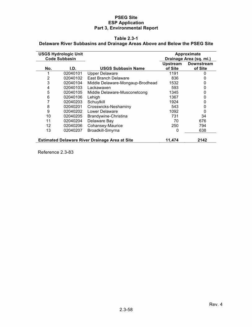
PSEG Site ESP Application
Part 3, Environmental Report
Rev. 4 2.3-58
Table 2.3-1 Delaware River Subbasins and Drainage Areas Above and Below the PSEG Site
USGS Hydrologic Unit
Code Subbasin
USGS Subbasin Name
Approximate Drainage Area (sq. mi.)
No. I.D. Upstream
of Site Downstream
of Site
1 02040101 Upper Delaware 1191 0 2 02040102 East Branch Delaware 836 0 3 02040104 Middle Delaware-Mongaup-Brodhead 1532 0 4 02040103 Lackawaxen 593 0 5 02040105 Middle Delaware-Musconetcong 1345 0 6 02040106 Lehigh 1367 0 7 02040203 Schuylkill 1924 0 8 02040201 Crosswicks-Neshaminy 543 0 9 02040202 Lower Delaware 1092 0
10 02040205 Brandywine-Christina 731 34 11 02040204 Delaware Bay 70 676 12 02040206 Cohansey-Maurice 250 794 13 02040207 Broadkill-Smyrna 0 638
Estimated Delaware River Drainage Area at Site 11,474 2142
Reference 2.3-83

PSEG Site ESP Application
Part 3, Environmental Report
Rev. 4 2.3-59
Table 2.3-2 Selected Point Precipitation Frequency Estimates (Inches)(a)
Average
Recurrence Interval (years)
5 Min 60 Min 24 Hours 7 Days 30 Days 60 Days
1 0.35 1.19 2.65 3.91 7.33 11.13 5 0.48 1.79 4.16 5.93 10.29 15.09
10 0.54 2.06 4.96 6.97 11.57 16.59 25 0.60 2.41 6.18 8.48 13.29 18.48
100 0.70 2.96 8.42 11.17 16.02 21.19 500 0.79 3.58 11.76 14.96 19.26 23.98
a) 39.460 North latitude, 75.508 West longitude
Reference 2.3-37
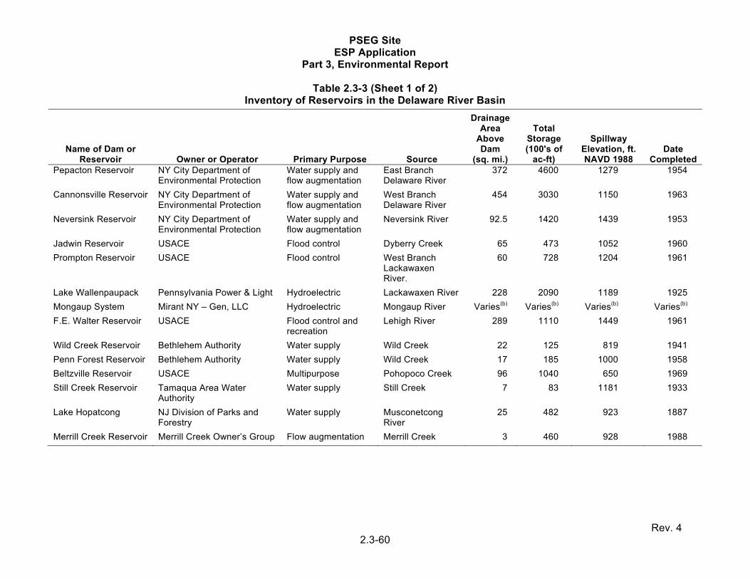
PSEG Site ESP Application
Part 3, Environmental Report
Rev. 4 2.3-60
Table 2.3-3 (Sheet 1 of 2) Inventory of Reservoirs in the Delaware River Basin
Name of Dam or Reservoir Owner or Operator Primary Purpose Source
Drainage Area
Above Dam
(sq. mi.)
Total Storage (100's of
ac-ft)
Spillway Elevation, ft. NAVD 1988
Date Completed
Pepacton Reservoir NY City Department of Environmental Protection
Water supply and flow augmentation
East Branch Delaware River
372 4600
1279 1954
Cannonsville Reservoir NY City Department of Environmental Protection
Water supply and flow augmentation
West Branch Delaware River
454 3030 1150 1963
Neversink Reservoir NY City Department of Environmental Protection
Water supply and flow augmentation
Neversink River 92.5 1420 1439 1953
Jadwin Reservoir USACE Flood control Dyberry Creek 65 473 1052 1960
Prompton Reservoir USACE Flood control West Branch Lackawaxen River.
60 728 1204 1961
Lake Wallenpaupack Pennsylvania Power & Light Hydroelectric Lackawaxen River 228 2090 1189 1925
Mongaup System Mirant NY – Gen, LLC Hydroelectric Mongaup River Varies(b) Varies(b) Varies(b) Varies(b)
F.E. Walter Reservoir USACE Flood control and recreation
Lehigh River 289 1110 1449 1961
Wild Creek Reservoir Bethlehem Authority Water supply Wild Creek 22 125 819 1941
Penn Forest Reservoir Bethlehem Authority Water supply Wild Creek 17 185 1000 1958
Beltzville Reservoir USACE Multipurpose Pohopoco Creek 96 1040 650 1969
Still Creek Reservoir Tamaqua Area Water Authority
Water supply Still Creek 7 83 1181 1933
Lake Hopatcong NJ Division of Parks and Forestry
Water supply Musconetcong River
25 482 923 1887
Merrill Creek Reservoir Merrill Creek Owner’s Group Flow augmentation Merrill Creek 3 460 928 1988
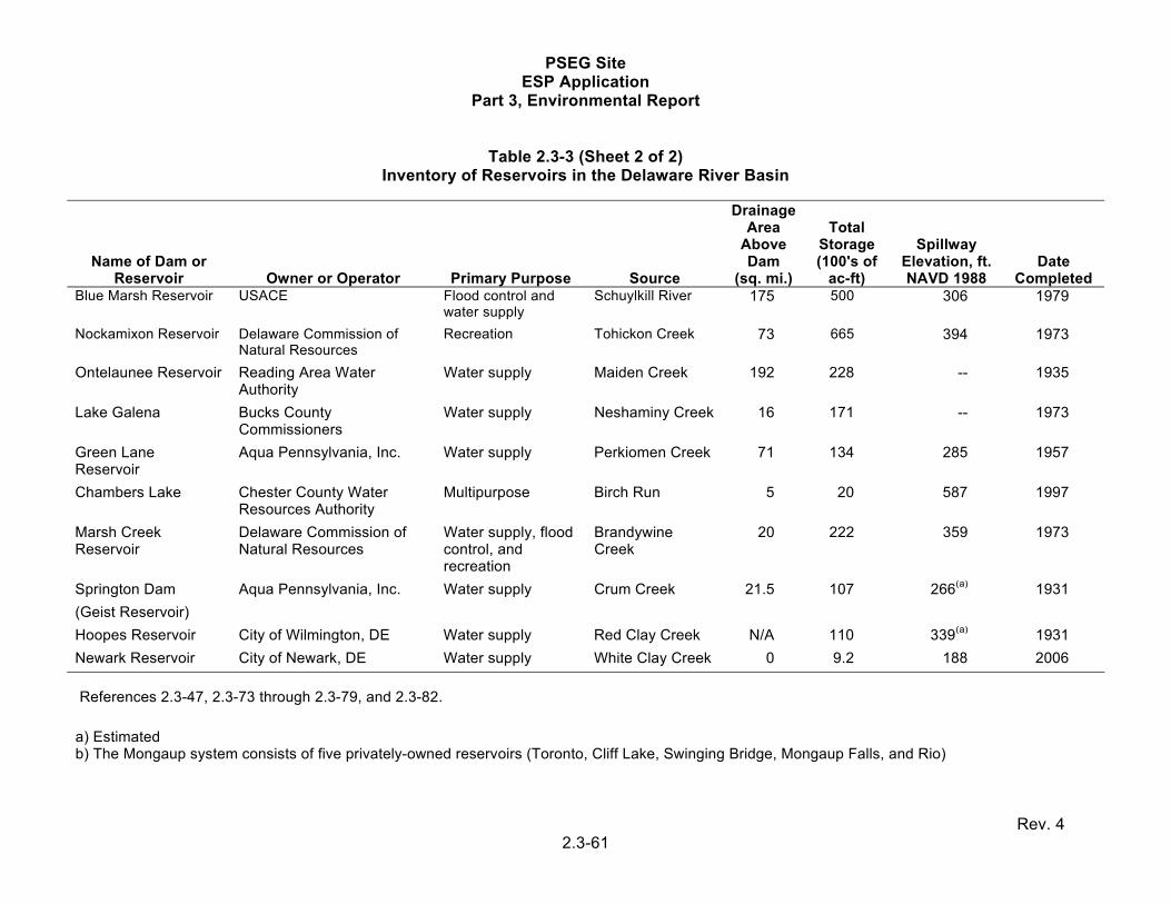
PSEG Site ESP Application
Part 3, Environmental Report
Rev. 4 2.3-61
Table 2.3-3 (Sheet 2 of 2)
Inventory of Reservoirs in the Delaware River Basin
Name of Dam or Reservoir Owner or Operator Primary Purpose Source
Drainage Area
Above Dam
(sq. mi.)
Total Storage (100's of
ac-ft)
Spillway Elevation, ft. NAVD 1988
Date Completed
Blue Marsh Reservoir USACE Flood control and water supply
Schuylkill River 175 500 306 1979
Nockamixon Reservoir Delaware Commission of Natural Resources
Recreation Tohickon Creek 73 665 394 1973
Ontelaunee Reservoir Reading Area Water Authority
Water supply Maiden Creek 192 228 -- 1935
Lake Galena Bucks County Commissioners
Water supply Neshaminy Creek 16 171 -- 1973
Green Lane Reservoir
Aqua Pennsylvania, Inc. Water supply Perkiomen Creek 71 134 285 1957
Chambers Lake Chester County Water Resources Authority
Multipurpose Birch Run 5 20 587 1997
Marsh Creek Reservoir
Delaware Commission of Natural Resources
Water supply, flood control, and recreation
Brandywine Creek
20 222 359 1973
Springton Dam
(Geist Reservoir)
Aqua Pennsylvania, Inc. Water supply Crum Creek 21.5 107 266(a) 1931
Hoopes Reservoir City of Wilmington, DE Water supply Red Clay Creek N/A 110 339(a) 1931
Newark Reservoir City of Newark, DE Water supply White Clay Creek 0 9.2 188 2006
References 2.3-47, 2.3-73 through 2.3-79, and 2.3-82.
a) Estimated b) The Mongaup system consists of five privately-owned reservoirs (Toronto, Cliff Lake, Swinging Bridge, Mongaup Falls, and Rio)

PSEG Site ESP Application
Part 3, Environmental Report
Rev. 4 2.3-62
Table 2.3-4 Tributary Streams in the Vicinity of the PSEG Site
Tributary Name Delaware River Mile
Lower Deep Creek 44
Mad Horse Creek 45
Fishing Creek 47
Hope Creek 48
Blackbird Creek 50
Appoquinimink River 51
Silver Run 53
Augustine Creek 53
Alloway Creek 54
St. Georges Creek 56
Salem River 58
Chesapeake and Delaware Canal 59
Mill Creek 60
Reference 2.3-22

PSEG Site ESP Application
Part 3, Environmental Report
Rev. 4 2.3-63
Table 2.3-5 Monthly and Annual Mean Daily Streamflow Statistics – Delaware River at
Trenton, New Jersey (Period of Record February 1, 1913 through May 3, 2009)
Period
Streamflow (cfs)
Streamflow (cfs) for Given Non-Exceedance Frequency
Mean Median (50%)
Minimum(0%) 10% 90%
Maximum(100%)
Annual 11,879 8100 1240 3070 24,800 279,000
January 12,772 9280 1900 4275 23,950 129,000
February 12,900 9860 2200 4850 24,810 110,000
March 20,563 16,500 3000 7506 36,680 214,000
April 22,165 18,000 4460 8959 39,200 230,000
May 13,970 11,600 3160 6096 24,800 139,000
June 9462 6800 1420 3889 16,800 224,000
July 7101 4920 1240 2700 12,700 110,000
August 6001 4210 1320 2300 10,800 279,000
September 6196 3940 1250 2170 11,100 181,000
October 7350 4380 1240 2260 15,050 121,000
November 10,760 7835 1240 2810 22,300 107,000
December 13,232 9690 1400 4000 26,800 118,000
Reference 2.3-87

PSEG Site ESP Application
Part 3, Environmental Report
Rev. 4 2.3-64
Table 2.3-6 Monthly Mean Streamflow Statistics – Delaware River at Trenton,
New Jersey (Period of Record October 1912 through September 2008)
Flow (cfs) Month Minimum Median Mean Maximum January 2539 11,595 12,916 34,950 February 3500 12,085 12,924 31,640 March 7715 19,295 20,627 60,840 April 6828 21,265 22,273 52,680 May 5074 12,100 13,977 31,690 June 2572 7176 9462 33,460 July 1548 5451 7101 25,720 August 1808 4442 6001 30,290 September 1762 4272 6196 32,570 October 1632 5105 7362 28,710 November 1868 10,440 10,765 27,340 December 2037 11,550 13,086 42,860 Reference 2.3-68

PSEG Site ESP Application
Part 3, Environmental Report
Rev. 4 2.3-65
Table 2.3-7 Flood Discharge Frequency – Alloway Creek
Location Drainage
Area (sq. mi.)
Peak Discharge (cfs)
10-year 50-year 100-year 500-year
At Confluence with Delaware River 59.6 2740 4520 5450 7800 At Salem-Hancocks Bridge Road 51.6 2440 4020 4850 6600
Reference 2.3-27

PSEG Site ESP Application
Part 3, Environmental Report
Rev. 4 2.3-66
Table 2.3-8 Summary of Selected Physical Features of the Delaware Estuary
Physical Feature Location / Statistic Measure
Length Falls at Trenton to Mouth of Bay
133.3 mi.
Width Minimum within Estuary 0.12 mi.
Maximum within Estuary 27 mi.
Depth Mean 19 ft.
Navigation Channel 30 – 40 ft.
Surface Area Open Water (Main Stem and Creeks)
758.7 sq. mi.
Marsh Plain Areas 246.8 sq. mi.
Total 1005.5 sq. mi.
Volume Total Estuary 4.5 x 10 11 ft3
Tidal Prism 1.4 x 10 11 ft3
Mean Tidal Range Cape May Point (RM 0) 4.8 ft.
Reedy Point (RM 54) 5.5 ft.
Trenton (RM 133) 8.1 ft.
Flow Tidal (Mouth of Bay) 5,190,000 cfs
Average Freshwater Inflow (total)
20,240 cfs
Watershed Total Area 13,533 sq. mi.
Estuary Drainage Area 5987 sq.mi.
Reference 2.3-54.

PSEG Site ESP Application
Part 3, Environmental Report
Rev. 4 2.3-67
Table 2.3-9 (Sheet 1 of 3) Regional and Site-Specific Aquifer Characteristics
Formation Transmissivity Hydraulic
Conductivity Total
Porosity Storage
Coefficient
Specific Capacity (gpm/ft)
Leakance (ft/d per ft.)
Reference
Fill 6.5 ft/d 2.3-1 Alluvium Aquifer
13.2 to 440 gpd/ft 0.9 to 13.1 gpd/ft2 2.3-71 2.95 ft/d 2.3-1
Kirkwood Aquitard
Kz = 0.00002 to
0.00005 ft/d 2.3-71
1e-5/d 2.3-84
Basal Kirkwood-Vincentown Aquifer
0.5 to 8.3 2.3-90 5000 to 11,000 gpd/ft 0.3 to 1.9 2.3-8
530 ft2/d 2.3-71 2000 to 2500 ft2/d 2.3-84 1987 to 2791 ft2/d 2.3-69
Hornerstown - Navesink Aquitard
30 to 65 gpd/ft2 0.522 – 0.543
2.3-90
Kz = 0.42 gpd/ft2 2.3-71
Kz = 0.005 to
9 ft/d 2.3-71
5e-5/d 2.3-84
3.35e-5 to 6.87e-5/d
2.3-69
Mount Laurel - Wenohah Aquifer
7000 gpd/ft 18.7 ft/d 2.3-13 10 ft/d 0.444 0.7 to 9 2.3-90
7500 to 14,000 gpd/ft 2.3-12 4900 to 8,700 gpd/ft 0.2 to 3.8 2.3-8
360 to 1.430 ft2/d 13 to 19 ft/d 2.3-71 1000 ft2/d 2.3-84
726 to 922 ft2/day 2.3-69

PSEG Site ESP Application
Part 3, Environmental Report
Rev. 4 2.3-68
Table 2.3-9 (Sheet 2 of 3) Regional and Site-Specific Aquifer Characteristics
Formation Transmissivity Hydraulic
Conductivity Porosity
Storage Coefficient
Specific Capacity (gpm/ft)
Leakance (ft/d per ft.)
Reference
Marshalltown-Wenohah Aquitard
0.001 to 0.01
gpd/ft2 2.3-90
Kz = 0.0000057 to
0.13 ft/d 2.3-71
6e-6/d 2.3-84
5.91e-6 to 7.13e-6/d
2.3-69
Englishtown Aquifer
up to 10 2.3-90 1100 to 2,100 ft2/d 12 to 67 ft/d 2.3-71
500 ft2/d 2.3-84 415 to 552 ft2/d 2.3-69
Merchantville-Woodbury Confining Unit
Kz = 0.00000087
to 0.03 ft/d 2.3-71
3e-6/d 2.3-84
2.15e-6 to 3.85e-6/d
2.3-69
Upper PRM Aquifer
10,000 to 25,000 gpd/ft
2.3-11
15,000 to 25,000 gpd/ft
2.3-9
9000 to 27,000 gpd/ft 10.6 to
26.7 2.3-8
870 to 24,210 gpd/ft 240 ft/d 2.3-71 2000 ft2/d 2.3-84
1086 to 2419 ft2/d 2.3-69

PSEG Site ESP Application
Part 3, Environmental Report
Rev. 4 2.3-69
Table 2.3-9 (Sheet 3 of 3) Regional and Site-Specific Aquifer Characteristics
Formation Transmissivity Hydraulic
Conductivity Porosity
Storage Coefficient
Specific Capacity (gpm/ft)
Leakance (ft/d per ft.)
Reference
Confining Unit, Upper to Middle PRM
Kz = 0.084 ft/d 2.3-71 2e-6/d 2.3-84
1.797e-7 to 2.69e-
7/d 2.3-69
Middle PRM Aquifer
4700 to 11,500 gpd/ft 2.3-11 8590 gpd/ft 129.5 ft/d 0.0025 2.3-44
670 to 4000 gpd/ft 2.3-8 4000 ft2/d 2.3-84
3024 to 3813 ft2/d 2.3-69 Confining Unit, Middle to Lower PRM
5e-6/d 2.3-84
7.19e-7 to 1.67e-5/d
2.3-69
Lower PRM Aquifer
2300 to 16,600 ft2/d 2.3-71 4000 to 5000 ft2/d 2.3-84 4844 to 5299 ft2/d 2.3-69
Kz = Vertical hydraulic conductivity. d = day Units of transmissivity in gallons per day per foot are converted to ft2/d by dividing by 7.48 gallons per cubic foot. Units of hydraulic conductivity in gallons per day per square foot are converted to ft/d by dividing by 7.48 gallons per cubic foot.

PSEG Site ESP Application
Part 3, Environmental Report
Rev. 4 2.3-70
Table 2.3-10 (Sheet 1 of 11) Summary of Public Water Supply Wells within a 25-Mile Radius of the PSEG Site(c)
Well Identification Owner County Total
Depth(a) Pump Rate
(gpm) New Jersey
NJGS0000000260 J & J Community Park Cumberland 0 14.6
NJGS0000000261 J & J Community Park Cumberland 0 14.6
NJGS0000000365 Handy's Mobile Park Salem 0 9
NJGS0000000366 Handy's Mobile Park Salem 0 20
NJGS0000000368 Country Club Estates Mobile Home Salem 0 0
WSWL0000066937 South Jersey Water Supply Co. Gloucester 270 250
WSWL0000066939 Penns Grove Water Supply Co. Gloucester 0 270
WSWL0000066944 Penns Grove Water Supply Co. Salem 371 400
WSWL0000067026 Woodstown Water Dept. Salem 0 600
WSWL0000067035 Penns Grove Water Supply Co. Salem 79 450
WSWL0000067056 NJ American Water Co. Gloucester 219 700
WSWL0000067059 Pennsville Township Water Dept. Salem 119 700
WSWL0000067065 Penns Grove Water Supply Co. Salem 62 250
WSWL0000067068 Penns Grove Water Supply Co. Gloucester 104 270
WSWL0000067075 Penns Grove Water Supply Co. Salem 96 300
WSWL0000067102 Pennsville Township Water Dept. Salem 106 700
WSWL0000067105 NJ American Water Co. Gloucester 166 0
WSWL0000067119 Harrisonville Mobile Home Park Gloucester 151 48
WSWL0000067142 Penns Grove Water Supply Co. Salem 87 250
WSWL0000067145 Swedesboro Water Dept. Gloucester 322 500
WSWL0000067147 South Jersey Water Supply Co. Gloucester 398 500
WSWL0000067153 NJ American Water Co. Gloucester 106 0
WSWL0000067154 Woodstown Water Dept. Salem 151 400
WSWL0000067168 Auburn Village Water Supply Salem 0 0

PSEG Site ESP Application
Part 3, Environmental Report
Rev. 4 2.3-71
Table 2.3-10 (Sheet 2 of 11) Summary of Public Water Supply Wells within a 25-Mile Radius of the PSEG Site(c)
Well Identification Owner County Total
Depth(a) Pump Rate
(gpm) New Jersey, cont.
WSWL0000067201 Woodstown Water Dept. Salem 1143.8 550
WSWL0000067202 Consumers NJ Water Co. Gloucester 240 0
WSWL0000067203 Consumers NJ Water Co. Gloucester 235 0
WSWL0000067213 South Jersey Water Supply Co. Gloucester 256 1200
WSWL0000067214 Salem Water Dept. Salem 171 250
WSWL0000067340 Elmer Borough Water Dept. Salem 573 400
WSWL0000067516 Picnic Grove Mobile Homes Salem 0 47
WSWL0000067529 Harding Woods Mobile Home Park Salem 0 180
WSWL0000067530 Harding Woods Mobile Home Park Salem 0 175
WSWL0000067634 Elmer Borough Water Dept. Salem 520 400
WSWL0000081691 Christy Enterprises Gloucester 310 12
WSWL0000065052 Fairton Trailer Park Cumberland 60 45
WSWL0000066928 Pennsville Township Water Dept. Salem 242 400
WSWL0000066988 Penns Grove Water Supply Co. Salem 84 500
WSWL0000067001 Auburn Village Water Supply Salem 270 100
WSWL0000067007 Swedesboro Water Dept. Gloucester 343 600
WSWL0000067021 NJ American Water Co. Gloucester 0 120
WSWL0000067022 NJ American Water Co. Gloucester 229 700
WSWL0000067545 Harrisonville Mobile Home Park Gloucester 247 70
WSWL0000067579 Picnic Grove Mobile Homes Salem 0 47
WSWL0000068642 Fairton Trailer Park Cumberland 59 20
WSWL0000068645 Bridgeton Water Dept. Cumberland 107 200
WSWL0000068652 Bridgeton Water Dept. Cumberland 126 500

PSEG Site ESP Application
Part 3, Environmental Report
Rev. 4 2.3-72
Table 2.3-10 (Sheet 3 of 11) Summary of Public Water Supply Wells within a 25-Mile Radius of the PSEG Site(c)
Well Identification Owner County Total
Depth(a) Pump Rate
(gpm) New Jersey, cont.
WSWL0000068666 Bridgeton Water Dept. Cumberland 136 500
WSWL0000068673 Bridgeton Water Dept. Cumberland 120 500
WSWL0000068684 Bridgeton Water Dept. Cumberland 152 800
WSWL0000068685 Bridgeton Water Dept. Cumberland 114 350
WSWL0000068686 Bridgeton Water Dept. Cumberland 193 350
WSWL0000068699 Leisure Arms Complex Salem 0 25
WSWL0000068700 Leisure Arms Complex Salem 0 25
WSWL0000068717 Tips Trailer Park & Sales Cumberland 70 60
WSWL0000068767 Tips Trailer Park & Sales Cumberland 0 40
WSWL0000068795 Upper Deerfield Township Water Dept. Cumberland 186 0
WSWL0000068800 Bridgeton Water Dept. Cumberland 110 0
WSWL0000068807 Bridgeton Water Dept. Cumberland 126 0
WSWL0000068809 Upper Deerfield Township Water Dept. Cumberland 196 0
WSWL0000068837 Seabrook Water Co. Cumberland 185 800
WSWL0000068881 Fairton Trailer Park Cumberland 52 45
WSWL0000069155 U.S. Dept of Justice/Federal Bureau of Prisons Cumberland 130 250
WSWL0000069166 U.S. Dept of Justice/Federal Bureau of Prisons Cumberland 120 250
WSWL0000069176 Millville Water Dept. Cumberland 153 700
WSWL0000069083 Holly Tree Acres Salem 0 30
WSWL0000069105 Holly Tree Acres Salem 137 30
WSWL0000069106 Holly Tree Acres Salem 137 30
WSWL0000070413 Swedesboro Water Dept. Gloucester 0 400
WSWL0000070414 Woodstown Water Dept. Salem 0 425
WSWL0000070417 Pennsville Township Water Dept. Salem 248 250

PSEG Site ESP Application
Part 3, Environmental Report
Rev. 4 2.3-73
Table 2.3-10 (Sheet 4 of 11) Summary of Public Water Supply Wells within a 25-Mile Radius of the PSEG Site(c)
Well Identification Owner County Total
Depth(a) Pump Rate
(gpm) New Jersey, cont.
WSWL0000070418 Salem Water Dept. Salem 157 500
WSWL0000070420 South Jersey Water Supply Co. Gloucester 285 120
WSWL0000070435 Penns Grove Water Supply Co. Salem 392 275
WSWL0000070444 Laux Lakeview Mobile Home Park Inc. Gloucester 0 100
WSWL0000070445 Laux Lakeview Mobile Home Park Inc. Gloucester 0 100
WSWL0000070446 Laux Lakeview Mobile Home Park Inc. Gloucester 0 65
WSWL0000070447 Laux Lakeview Mobile Home Park Inc. Gloucester 0 100
WSWL0000070835 Bridgeton Water Dept. Cumberland 93 525
WSWL0000070838 Seabrook Water Co. Cumberland 0 600
WSWL0000070839 Seabrook Water Co. Cumberland 0 600
WSWL0000070888 Tips Trailer Park & Sales Cumberland 0 0
WSWL0000070889 Tips Trailer Park & Sales Cumberland 0 40
WSWL0000078126 Consumers NJ Water Co. Gloucester 0 350
WSWL0000078127 Consumers NJ Water Co. Gloucester 0 350
WSWL0000091158 South Jersey Water Supply Co. Gloucester 270 1200
WSWL0000138942 Bridgeton Water Dept. Cumberland 94 0
WSWL0000138947 Bridgeton Water Dept. Cumberland 400 500
WSWL0000138948 Bridgeton Water Dept. Cumberland 0 500
WSWL0000138949 Salem Water Dept. Salem 165 324
WSWL0000138950 Bridgeton Water Dept. Cumberland 405 500
WSWL0000139268 Bridgeton Water Dept. Cumberland 108 0
WSWL0000139269 Bridgeton Water Dept. Cumberland 92 0
WSWL0000176817 Pennsville Township Water Dept. Salem 153 0

PSEG Site ESP Application
Part 3, Environmental Report
Rev. 4 2.3-74
Table 2.3-10 (Sheet 5 of 11) Summary of Public Water Supply Wells within a 25-Mile Radius of the PSEG Site(c)
Well Identification Owner County Total
Depth(a) Pump Rate
(gpm) New Jersey, cont.
WSWL0000176818 Pennsville Township Water Dept. Salem 269 0
WSWL0000190792 NJ American Water Co. Gloucester 105 700
WSWL0000191667 Hopewell Place Senior Apartments Cumberland 82 75
WSWL0000191528 Holly Tree Acres Salem 0 20
WSWL0000191530 Fairton Trailer Park Cumberland 60 0
WSWL0000191565 Picnic Grove Mobile Homes Salem 0 24
WSWL0000191567 Country Club Estates Mobile Home Salem 0 50
WSWL0000191568 Harrison Mobile Park Salem 93 25
WSWL0000191573 Harrison Mobile Park Salem 0 25
WSWL0000191681 Handy's Mobile Park Salem 187 30
WSWL0000191682 Harding Woods Mobile Home Park Salem 105 200
WSWL0000215097 Seabrook Water Co. Cumberland 335 30
WSWL0000215958 Pennsville Township Water Dept. Salem 0 500
WSWL0000293710 Country Club Estates Mobile Home Salem 0 15
WSWL0000454591 Rainbow Convalescent Center Salem 88 30
WSWL0000475741 Rainbow Convalescent Center Salem 90 30
WSWL0000708077 J & J Community Park Cumberland 563 20
WSWL0000824635 Pennsville Township Water Dept. Salem 0 500
WSWL0000831109 Woodstown Water Dept. Salem 155 200
WSWL0000842061 Penns Grove Water Supply Co. Salem 0 275

PSEG Site ESP Application
Part 3, Environmental Report
Rev. 4 2.3-75
Table 2.3-10 (Sheet 6 of 11) Summary of Public Water Supply Wells within a 25-Mile Radius of the PSEG Site(c)
Well Identification Owner Watershed Total
Depth(a) Pump Rate
(gpm) Delaware
84445 St. Georges C & D Canal East 142 10
168612 DelDOT Dragon Run Creek 59 10
69050 Hollingsworth, Diamond State Dragon Run Creek 250 10
69051 Petroleum, Eastern Dragon Run Creek 160 10
69052 Stapleford, Charles Sr. Dragon Run Creek 302 10
90632 Parkway Gravel Inc. C & D Canal East 160 30
171554 Edwards, Richard Red Lion Creek 85 10
177079 71 Holding Company C & D Canal East 275 15
65280 Madic Inc., Michael C & D Canal East 76 20
63015 Thirty Three, Forty Limited C & D Canal East 37 10
80752 Motiva Enterprises LLC Red Lion Creek 45 10
77305 St Georges Association Dragon Run Creek 275 20
94029 DelDOT Dragon Run Creek 64 20
79910 Blaschko, John W. Red Lion Creek 50 10
90632 Parkway Gravel Inc. C & D Canal East 160 30
91916 Parkway Gravel C & D Canal East 200 30
96341 Blaschko, John W. Red Lion Creek 35 10
102661 Buttocoula, Louis Appoquinimink River 152 10
192969 Whiteman, Marty Appoquinimink River 125 10
102872 Genes Body Shop Appoquinimink River 39 10
103777 New Castle County Appoquinimink River 190 60
105016 Hearne, William A. Appoquinimink River 200 0
107232 Whiteman, Mike Appoquinimink River 100 50

PSEG Site ESP Application
Part 3, Environmental Report
Rev. 4 2.3-76
Table 2.3-10 (Sheet 7 of 11) Summary of Public Water Supply Wells within a 25-Mile Radius of the PSEG Site(c)
Well Identification Owner Watershed Total
Depth(a) Pump Rate
(gpm) Delaware, cont.
105151 Zoar Methodist Church Appoquinimink River 201 20
154043 Glorious Church of God Blackbird Creek 140 20
158489 Frog Hollow LLC Appoquinimink River 162 30
161541 Artesian Water Company Inc. Appoquinimink River 118 20
167920 McKeown, Robert Appoquinimink River 157 10
185045 Stanley Builders Appoquinimink River 184 10
190088 Delaware Solid Waste Authority Blackbird Creek 132 20
204315 Averill, Ron Blackbird Creek 70 10
202974 New Castle County Appoquinimink River 121 20
36214 Wyoming Block Co. Blackbird Creek 157 60
50682 Tappahanna Blackbird Creek 30 5
62905 Mummford & Miller, Concrete Appoquinimink River 200 20
72425 Salvage, Fred D. Blackbird Creek 150 20
74671 Calotex, Delaware Inc. Blackbird Creek 120 10
77049 Middletown Seventh-Day Adventist Appoquinimink River 95 20
77648 Mumford & Mille Appoquinimink River 90 10
83331 Harvey & Harvey Blackbird Creek 130 20
91490 DEL DOT Div of Highways Appoquinimink River 118 10
43962 Kirkwood Soccer Club Army Creek 215 900
43963 Artesian Water Company Inc. Army Creek 225 300
101760 Artesian Water Company Inc. Army Creek 170 700
103480 Crab Rib C & D Canal East 105 10
106649 United Water Delaware Dragon Run Creek 295 25

PSEG Site ESP Application
Part 3, Environmental Report
Rev. 4 2.3-77
Table 2.3-10 (Sheet 8 of 11) Summary of Public Water Supply Wells within a 25-Mile Radius of the PSEG Site(c)
Well Identification Owner Watershed Total
Depth(a) Pump Rate
(gpm) Delaware, cont.
194042 Parkway Gravel Red Lion Creek 152 25
194043 Parkway Gravel Red Lion Creek 187 25
194044 Parkway Gravel Red Lion Creek 402 25
36504 City of Delaware City Dragon Run Creek 720 300
62314 Chesapeake, Canal Partners C & D Canal East 280 10
83253 Colonial School Dragon Run Creek 350 30
88603 Mullins, William F. C & D Canal East 80 20
80405 Shopping Center (undesignated) Dragon Run Creek 120 20
78555 Carroll, Chester Dragon Run Creek 250 20
80167 Colonial School, Dragon Run Creek 700 0
10429 State of DE DAS/DFM C & D Canal East 190 100
90048 Crab Rib C & D Canal East 120 20
99719 U.S. Postal Service Army Creek 208 10
1(b) Gunning Bedford Dragon Run Creek 341 0
169693 Diamond State Realty Co. C & D Canal East 125 20
89283 Farm Land Holdings LLC C & D Canal East 125 30
89284 Farm Land Holdings LLC C & D Canal East 135 30
89285 Farm Land Holdings LLC C & D Canal East 130 30
101153 Stanley Builders C & D Canal East 505 300
102151 Artesian Water Company Inc C & D Canal East 400 400
102224 Hickey, John & Amy C & D Canal East 135 10
104063 U.S. Army Corps of Engineers C & D Canal East 268 20
105156 Artesian Water Company Inc. C & D Canal East 495 100

PSEG Site ESP Application
Part 3, Environmental Report
Rev. 4 2.3-78
Table 2.3-10 (Sheet 9 of 11) Summary of Public Water Supply Wells within a 25-Mile Radius of the PSEG Site(c)
Well Identification Owner Watershed Total
Depth(a) Pump Rate
(gpm) Delaware, cont.
105157 Davis, Leola B. C & D Canal East 792 0
156288 Artesian Water Company Inc. C & D Canal East 625 50
162618 Artesian Water Company Inc. C & D Canal East 152 0
199537 Tidewater Utilities C & D Canal East 170 0
41871 Lester, Earl C & D Canal East 80 30
39786 Mazik, Ken Dragon Run Creek 289 20
53347 Buckson, Newlin C & D Canal East 37 10
43368 Reybold Homes Dragon Run Creek 240 80
68944 Tidewater Utilities, Inc. C & D Canal East 80 0
68945 Norfolk Southern Railroad C & D Canal East 230 75
59152 Walker, Guy C & D Canal East 165 20
54126 Mt. Pleasant Trailer Park C & D Canal East 45 25
75180 Common Wealth C & D Canal East 115 10
78973 Tidewater Utilities, Inc. C & D Canal East 160 160
99469 Artesian Water Company Inc. C & D Canal East 534 580
82242 Tidewater Utilities, Inc. C & D Canal East 80 160
82244 Tidewater Utilities, Inc. C & D Canal East 95 160
74785 Gentlemens Farmers Rest Inc. C & D Canal East 103 150
84135 Tidewater Utilities, Inc. C & D Canal East 120 0
10757 Commodore Macdo Dragon Run Creek 35 0
1202 DNREC-Fish & Wildlife C & D Canal East 105 0
98112 Artesian Water Company C & D Canal East 300 0
93214 New Group Investments Appoquinimink River 160 30

PSEG Site ESP Application
Part 3, Environmental Report
Rev. 4 2.3-79
Table 2.3-10 (Sheet 10 of 11) Summary of Public Water Supply Wells within a 25-Mile Radius of the PSEG Site(c)
Well Identification Owner Watershed Total
Depth(a) Pump Rate
(gpm) Delaware, cont.
99806 Artesian Water Company Inc. Appoquinimink River 740 800
102217 Gilchrist, Robert A. Appoquinimink River 200 80
109874 Artesian Water Company Inc. Appoquinimink River 435 0
110612 Artesian Water Company Inc. Appoquinimink River 330 200
108202 Artesian Water Company Inc. Appoquinimink River 450 300
111065 Artesian Water Company Inc. Appoquinimink River 740 300
111968 Artesian Water Company Inc. Appoquinimink River 238 0
168004 Conoco, Inc. Appoquinimink River 220 15
178412 St Andrews School of DE, Inc. Appoquinimink River 389 15
188292 Artesian Water Company Inc. Appoquinimink River 983 550
179292 Tidewater Utilities, Inc. Appoquinimink River 180 90
185186 Artesian Water Company Inc. Appoquinimink River 300 250
185232 Tidewater Utilities, Inc. Appoquinimink River 230 75
196919 Artesian Water Company Inc. Blackbird Creek 300 250
39676 Town of Middletown Appoquinimink River 846 250
37195 New Castle County Appoquinimink River 70 25
58805 Pre Holding Hampstead LLC Appoquinimink River 201 35
53259 Bailey, James Blackbird Creek 310 20
72100 Justice of the Peace Appoquinimink River 118 10
89852 Reed, Charolet Appoquinimink River 170 40
70172 Howard Cohen, Middletown Appoquinimink River 165 25
82787 Diamond Appoquinimink River 201 20
10454 Wicks, Christopher Appoquinimink River 375 250

PSEG Site ESP Application
Part 3, Environmental Report
Rev. 4 2.3-80
Table 2.3-10 (Sheet 11 of 11) Summary of Public Water Supply Wells within a 25-Mile Radius of the PSEG Site(c)
Well Identification Owner Watershed Total
Depth(a) Pump Rate
(gpm) Delaware, cont.
10745 Cantwell Water Appoquinimink River 228 0
10746 Cantwell Water Appoquinimink River 168 0
10765 Children Castle Appoquinimink River 150 0
10766 St Andrews School of DE, Inc Appoquinimink River 650 0
10767 St Andrews School of DE, Inc Appoquinimink River 181 0
10772 Delaware State Appoquinimink River 206 0
71254 Tidewater Utilities, Inc. Appoquinimink River 163 250
96299 Tidewater Utilities, Inc. C & D Canal East 160 150
96300 Tidewater Utilities, Inc. C & D Canal East 170 150
98363 Fas Mart Blackbird Creek 160 10
30021 Camp Ground Inco, Delmarva Blackbird Creek 165 0
30022 Williams Assoc. Blackbird Creek 178 0
97960 Tidewater Utilities, Inc. Appoquinimink River 220 80
33392 Hampson, Leonora Appoquinimink River 200 50
84852 Reed, Charolet Appoquinimink River 160 40
585 South Market Appoquinimink River 200 0
30148 Townsend Blackbird Creek 206 150
10099 City of Delaware City Dragon Run Creek 235 100
58900 Odessa Motel, Larry Cox Appoquinimink River 201 20
a) Depths provided in feet below ground surface. b) Permit number presented as in the DE DNR database, however, the number is likely an error. c) Public water supply wells within DE and NJ not inclusive of wells that are mapped in wellhead protection areas. Wellhead protection areas
in DE and NJ are shown on Figure 2.3-20. References 2.3-39 and 2.3-25

PSEG Site ESP Application
Part 3, Environmental Report
Rev. 4 2.3-81
Table 2.3-11 (Sheet 1 of 8) Summary of Groundwater Users within the 25-Mile Radius(b)
Program
ID Program Interest Name Activity
Number(a) Activity type Description
Effective Start Date
Expiration Date
Gloucester County, NJ 2029P Air Products & Chemicals Inc. WAP980001 Water Allocation Permit - Renewal 6/23/1999 12/31/2010
5383 Aqua New Jersey Inc. (Woolwich) WAP050002 Water Allocation Permit - Minor Modification
1/1/2006 12/31/2010
2272P Beckett Golf Club Inc. WAP990001 Water Allocation Permit - Renewal 10/30/2002 12/31/2010
2401P BP Terminal No. 4555 WAP070001 Water Allocation Permit - Renewal 12/1/2008 11/30/2018
2530P Bridgeport Disposal LLC WAP050001 Water Allocation Permit - Minor Modification
6/1/2005 4/30/2014
2495E Chemical Leaman Tanklines EQP080001 Water Allocation Permit Equivalency - Renewal
10/1/2008 9/30/2018
5244 Clayton Borough Water Dept. WAP040001 Water Allocation Permit - Modification 4/1/2005 3/31/2015
2014P Colonial Estates WAP080001 Water Allocation Permit - Renewal 11/1/2008 10/31/2018
5336 Deptford Township Municipal Utilities Authority
WAP070001 Water Allocation Permit - Administrative Modification
5/1/2007 12/31/2010
5142 East Greenwich Township WAP060001 Water Allocation Permit - Renewal 1/1/2007 12/31/2016
2251P E.I. Dupont Denemours & Company Inc. Repauno Plant
WAP040002 Water Allocation Permit - Renewal 9/1/2005 8/31/2015
2099P Ferro Corp WAP070001 Water Allocation Permit - Minor Modification
5/9/2007 7/31/2014
5135 Glassboro Borough Water Dept. WAP080001 Water Allocation Permit - Renewal 11/1/2008 10/31/2018
2280P Gloucester County Pitman Golf Course
WAP030001 Water Allocation Permit - Renewal 10/1/2004 12/31/2013
2423P Grasso Foods Inc. WAP990001 Water Allocation Permit - Renewal 6/30/2000 12/31/2010

PSEG Site ESP Application
Part 3, Environmental Report
Rev. 4 2.3-82
Table 2.3-11 (Sheet 2 of 8)
Summary of Groundwater Users within the 25-Mile Radius(b)
Program ID Program Interest Name
Activity Number(a)
Activity type Description Effective
Start Date Expiration
Date Gloucester County, NJ, cont.
5253 Greenwich Township Water Dept. WAP000001 Water Allocation Permit - Renewal 10/19/2001 12/31/2010
2469E Helen Kramer Landfill Superfund Site
EQP080001 Water Allocation Permit Equivalency - Renewal
10/1/2008 9/30/2018
2227P Hercules Groundwater Treatment WAP070002 Water Allocation Permit - Minor Modification
1/1/2008 4/30/2012
2391P Inversand Co. WAP960001 Water Allocation Permit - Renewal 1/20/1998 12/31/2010
4059PS Logan Generating Company LP WAP050001 Water Allocation Permit - Renewal 11/1/2006 10/31/2016
5314 Mantua Township Municipal Utilities Authority
WAP080001 Water Allocation Permit - Minor Modification
9/1/2008 6/30/2012
2291P Maple Ridge Golf Course WAP010001 Water Allocation Permit - Renewal 10/24/2002 12/31/2011
5161 Monroe Township Municipal Utilities Authority
WAP050001 Water Allocation Permit - Modification 6/1/2007 5/31/2017
5153 National Park Borough Water Dept.
WAP070001 Water Allocation Permit - Renewal 4/1/2008 3/31/2018
5147 Newfield Borough Water Dept. WAP030001 Water Allocation Permit - Renewal 8/1/2004 6/30/2014
5375 NJ American Water - Bridgeport WAP070001 Water Allocation Permit - Modification 8/1/2008 7/31/2018
5183 NJ American Water - Harrison WAP070002 Water Allocation Permit - Hearing Appeal Modification
4/1/2008 7/31/2017
5003 NJ American Water Logan System
WAP030001 Water Allocation Permit - Renewal 3/1/2004 12/31/2013

PSEG Site ESP Application
Part 3, Environmental Report
Rev. 4 2.3-83
Table 2.3-11 (Sheet 3 of 8)
Summary of Groundwater Users within the 25-Mile Radius(b)
Program ID Program Interest Name
Activity Number(a)
Activity type Description Effective
Start Date Expiration
Date Gloucester County, NJ, cont.
2425P Nustar Asphalt Refining LLC WAP040001 Water Allocation Permit - Minor Modification
9/1/2005 10/31/2012
5130 Paulsboro Water Dept. WAP070001 Water Allocation Permit - Renewal 10/1/2007 9/30/2017
5137 Pitman Borough Water Dept. WAP000001 Water Allocation Permit - Renewal 10/30/2002 2/28/2011
2215P Preferred Real Estate Investments
WAP060001 Water Allocation Permit - Renewal 4/1/2007 3/31/2012
2336P RE Pierson Materials Corp. WAP020001 Water Allocation Permit - Renewal 9/1/2003 2/28/2013
4073PS River Winds at West Deptford WAP990001 Water Allocation Permit - New 4/17/2003 11/30/2012
2543P Sahara Sand ff Franklin Inc. WAP020001 Water Allocation Permit - New 3/26/2003 11/30/2012
2234P Solvay Solexis Inc. WAP080001 Water Allocation Permit - Modification 4/1/2009 3/31/2019
2205P Sunoco Inc. (R&M) Eagle Point Facility
WAP060001 Water Allocation Permit - Administrative Modification
10/1/2006 6/30/2015
5105 Swedesboro Water Dept. WAP010001 Water Allocation Permit - Renewal 11/26/2001 10/31/2011
2424E USEPA Lipari Landfill Superfund Site
EQP910001 Water Allocation Permit Equivalency - New
12/2/1991
2204P Valero Refining Co. - NJ WAP070002 Water Allocation Permit - Renewal 7/1/2008 6/30/2018
1281D Valero Refining Co. NJ DWP080001 Temporary Dewatering Permit - New 6/1/2009 7/31/2012
2177P Violet Packing LLC WAP980001 Water Allocation Permit - Renewal 12/30/1999 12/31/2010
5194 Washington Township Municipal Utilities Association
WAP060001 Water Allocation Permit - Modification 2/1/2008 1/31/2018
5192 Wenonah Borough Water Dept. WAP010001 Water Allocation Permit - Renewal 9/11/2002 1/31/2011

PSEG Site ESP Application
Part 3, Environmental Report
Rev. 4 2.3-84
Table 2.3-11 (Sheet 4 of 8)
Summary of Groundwater Users within the 25-Mile Radius(b)
Program ID Program Interest Name
Activity Number(a)
Activity type Description Effective
Start Date Expiration
Date Gloucester County, NJ, cont.
5304 West Deptford Township - Public Works
WAP050001 Water Allocation Permit - Renewal 11/1/2006 10/31/2016
5319 Westville Borough Water Dept. WAP000001 Water Allocation Permit - Renewal 1/31/2003 12/31/2010
2257P Westwood Golf Club WAP060001 Water Allocation Permit - Renewal 5/1/2007 4/30/2017
2365P Wheelabrator Gloucester Co. LP WAP980001 Water Allocation Permit - Renewal 12/30/1999 12/31/2010
5347X Woodbury City Water Dept WAP030001 Water Allocation Permit - Renewal 9/1/2004 8/31/2012
5347X Woodbury City Water Dept WAP990001 Water Allocation Permit - Modification 9/1/2004 8/31/2012
5159 Woodbury Heights Borough Water Utility
WAP060001 Water Allocation Permit - Renewal 4/1/2007 3/31/2017
Salem County, NJ
2413P B & B Poultry Co. Inc. WAP060001 Water Allocation Permit - Renewal 12/1/2007 11/30/2017
2104P Deepwater Generating Station WAP980001 Water Allocation Permit - Renewal 3/20/2001 12/31/2010
2122P Dupont Chambers Works WAP070002 Water Allocation Permit - Minor Modification
11/1/2007 5/31/2012
5215 Elmer Borough Water Dept. WAP990001 Water Allocation Permit - Renewal 12/1/2003 11/30/2013
5170 Harding Woods Mobile Home Park
WAP040001 Water Allocation Permit - Administrative Modification
7/29/1999 2/28/2009
5328 NJ American Water - Pennsgrove WAP070002 Water Allocation Permit - Minor Modification
6/1/2007 7/31/2016
2421P Pedricktown Cogeneration Company
WAP070001 Water Allocation Permit - Renewal 7/1/2008 6/30/2018

PSEG Site ESP Application
Part 3, Environmental Report
Rev. 4 2.3-85
Table 2.3-11 (Sheet 5 of 8)
Summary of Groundwater Users within the 25-Mile Radius(b)
Program ID Program Interest Name
Activity Number(a)
Activity type Description Effective
Start Date Expiration
Date Salem County, NJ, cont.
5047 Pennsville Township Water Dept. WAP020001 Water Allocation Permit - Modification 10/1/2005 9/30/2015
2166P Polyone Corp. WAP080001 Water Allocation Permit - Minor Modification
12/1/2008 12/30/2014
2216P Salem and Hope Creek Generating Station
WAP040001 Water Allocation Permit - Minor Modification
1/1/2005 1/31/2010
5290 Salem City Water Dept. WAP020001 Water Allocation Permit - Modification 5/1/2005 3/31/2015
2528P Town & Country Golf Links WAP010001 Water Allocation Permit - New 1/1/2006 12/31/2015
2497P Wild Oaks Country Club WAP050001 Water Allocation Permit - Renewal 5/1/2007 4/30/2012
5167 Woodstown Borough Water Dept. WAP070001 Water Allocation Permit - Modification 6/1/2009 5/31/2019
Cumberland County, NJ
2095P Alcan Packaging Inc. WAP070001 Water Allocation Permit - Minor Modification
8/1/2008 6/30/2012
2010P Atlantic Coast Freezers WAP080001 Water Allocation Permit - Renewal 10/1/2008 9/30/2018
5398 Berrymans Branch Mobile Home Park
WAP070001 Water Allocation Permit - New 7/1/2008 6/30/2018
5032 Bridgeton City Water Dept. WAP980001 Water Allocation Permit - Modification 8/1/2003 1/31/2013
2448P Cape May Foods LLC doing business as Lamonica Fine Foods
WAP020001 Water Allocation Permit - Renewal 11/1/2003 9/30/2012

PSEG Site ESP Application
Part 3, Environmental Report
Rev. 4 2.3-86
Table 2.3-11 (Sheet 6 of 8)
Summary of Groundwater Users within the 25-Mile Radius(b)
Program ID Program Interest Name
Activity Number(a)
Activity type Description Effective
Start Date Expiration
Date Cumberland County, NJ, cont.
2220P Clement Pappas Co. Inc. WAP010001 Water Allocation Permit - Renewal 9/27/2002 1/31/2011
5364 Fairton Federal Correctional Institute
WAP970001 Water Allocation Permit - Renewal 12/23/1997 12/31/2010
5399 Fairview Manor Mobile Home Park
WAP070001 Water Allocation Permit - New 5/1/2008 4/30/2018
2552P Gerresheimer Glass Inc. WAP030001 Water Allocation Permit - Minor Modification
8/12/2004 7/31/2014
2254P Hanson Aggregates WAP990001 Water Allocation Permit - Modification 3/26/2003 12/31/2012
2098P Kimble Glass Inc. WAP980001 Water Allocation Permit - Renewal 6/14/2002 12/31/2010
2436P Mays Landing Sand & Gravel Co. Dorchester Plant
WAP070001 Water Allocation Permit - Renewal 3/1/2008 2/28/2018
5316 Millville City Water Dept. WAP980001 Water Allocation Permit - Renewal 9/10/2002 6/30/2011
2467E Nascolite (Potentially Responsible Parties) Group
EQP950001 Water Allocation Permit Equivalency - New
3/24/1995
5367 NJ State Prison Bayside WAP980001 Water Allocation Permit - Modification 2/21/2002 3/31/2010
2443P Purex Industries WAP010001 Water Allocation Permit - Renewal 10/30/2002 10/31/2011
2030P Ricci Brothers Sand Co. WAP070001 Water Allocation Permit - Minor Modification
5/1/2007 5/31/2016
2221P Seabrook Farms WAP050001 Water Allocation Permit - Renewal 4/1/2006 3/31/2016
2237P Shieldalloy Metallurgical Corp. WAP060001 Water Allocation Permit - Renewal 8/1/2007 7/31/2017
2440P South State Inc. WAP980001 Water Allocation Permit - Renewal 12/29/1998 12/31/2010

PSEG Site ESP Application
Part 3, Environmental Report
Rev. 4 2.3-87
Table 2.3-11 (Sheet 7 of 8)
Summary of Groundwater Users within the 25-Mile Radius(b)
Program ID Program Interest Name
Activity Number(a)
Activity type Description Effective
Start Date Expiration
Date Cumberland County, NJ, cont.
2219P Unimin Corp WAP050002 Water Allocation Permit - Renewal 7/1/2006 6/30/2016
5376 Upper Deerfield Township WAP070001 Water Allocation Permit - Modification 4/1/2008 3/31/2018
2485E USEPA Region II Vineland Chemical Co. Superfund
EQP070002 Water Allocation Permit Equivalency - Modification
8/1/2008 7/31/2018
2003P US Silica Co WAP040001 Water Allocation Permit - Modification 4/1/2005 3/31/2015
2282P US Silica Co. Port Elizabeth Plant WAP080001 Water Allocation Permit - Renewal 7/1/2008 6/30/2018
5148 Vineland City Water Utility WAP060001 Water Allocation Permit - Modification 8/1/2007 7/31/2017
2405P Vineland Kosher Poultry Co. WAP040001 Water Allocation Permit - Minor Modification
5/1/2004 12/31/2010
2026P Whibco Inc. WAP970001 Water Allocation Permit - Renewal 6/30/1997 5/31/2008
Delaware
53066 Star Enterprises NA Dragon Run Creek 2/1/1983 10/24/1983
53066 Star Enterprises NA Dragon Run Creek 2/1/1983 10/24/1983
216229 Highland View LLC NA Dragon Run Creek 10/3/2006 3/2/2007
216229 Highland View LLC NA Dragon Run Creek 10/3/2006 3/2/2007
10059 Motiva Enterprises LLC NA Dragon Run Creek 1/1/1956 1/1/1956
10059 Motiva Enterprises LLC NA Dragon Run Creek 1/1/1956 1/1/1956

PSEG Site ESP Application
Part 3, Environmental Report
Rev. 4 2.3-88
Table 2.3-11 (Sheet 8 of 8)
Summary of Groundwater Users within the 25-Mile Radius(b)
Program ID Program Interest Name
Activity Number(a)
Activity type Description Effective
Start Date Expiration
Date Delaware, cont.
43962 Kirkwood Soccer Club NA Army Creek 7/23/1979 9/17/1979
163874 Motiva Enterprises LLC NA Dragon Run Creek 2/19/1999 9/16/1999
163874 Motiva Enterprises LLC NA Dragon Run Creek 2/19/1999 9/16/1999
a) NA – “Activity numbers” are not a Delaware Department of Natural Resources database field b) Public water supply wells within DE and NJ. Summary includes permitted groundwater use of greater than 100,000 gallons per day. References 2.3-25 and 2.3-39

PSEG Site ESP Application
Part 3, Environmental Report
Rev. 4 2.3-89
Table 2.3-12 Observation Well Installation Details
Well ID Northing NAD83(b)
Easting NAD83(b)
Screen Interval (ft. bgs)
Reference Point
Elevation(a) (ft. NAVD 88)
Formation
New Plant Location NOW-1U 234542.7 198443.4 46-56 15.20 Alluvium NOW-1L 234564.0 198449.8 80-90 15.19 Vincentown NOW-2U 235207.4 197754.9 52-62 10.80 Alluvium NOW-2L 235227.7 197752.8 103-113 11.18 Vincentown NOW-3U 234552.8 197885.2 40-50 7.71 Alluvium NOW-3L 234565.5 197897.9 90-100 7.66 Vincentown NOW-4UB 233963.0 198147.1 42-52 13.56 Alluvium NOW-4L 233972.7 198147.9 73-83 14.08 Vincentown NOW-5U 234907.5 198444.5 20-30 10.23 Hydraulic Deposits NOW-5L 234927.5 198438.4 90-100 10.54 Vincentown NOW-6U 235269.4 198313.5 35-45 8.59 Alluvium NOW-6L 235287.9 198312.8 80-90 7.95 Vincentown NOW-7U 234975.8 199694.3 48-58 8.25 Alluvium /
Vincentown Boundary
NOW-7L 234973.4 199675.9 85-95 8.70 Vincentown NOW-8U 234141.6 199755.9 37-47 11.68 Alluvium NOW-8L 234139.1 199736.2 100-110 11.61 Vincentown Eastern Location EOW-1U 232321.6 202758.0 38-48 18.01 Alluvium EOW-1L 232297.6 202758.1 95-105 17.91 Vincentown EOW-2U 233274.6 202157.9 39-49 16.51 Alluvium EOW-2L 233271.5 202177.7 99-109 16.73 Vincentown EOW-4U 231791.9 202012.1 22-32 22.73 Hydraulic Deposits EOW-4L 231772.9 202021.2 110.2-120.2 22.31 Vincentown EOW-5U 233056.8 203007.3 35-45 15.85 Alluvium EOW-5L 233039.7 203021.5 110-120 16.17 Vincentown EOW-6U 232587.1 203281.4 47-57 15.99 Alluvium EOW-6L 232588.1 203300.7 90-100 15.23 Vincentown EOW-8U 231144.2 203520.4 30-40 18.38 Alluvium EOW-8L 231163.5 203516.0 67-77 17.89 Vincentown EOW-9U 230917.2 202826.0 50-60 20.67 Alluvium EOW-9L 230925.6 202844.6 117.5-127.5 18.21 Vincentown EOW-10U 231687.2 203521.3 17-27 14.79 Alluvium EOW-10L 231706.7 203521.9 85-95 14.27 Vincentown
ft. bgs = feet below ground surface, determined from well installation records a) Reference point elevation includes any modifications made to well riser b) NJ State Plane Coordinate System; U.S. Survey Feet

PSEG Site ESP Application
Part 3, Environmental Report
Rev. 4 2.3-90
Table 2.3-13 Groundwater Elevations (ft. NAVD), January to December 2009
Jan Feb Mar Apr May Jun Jul Aug Sept Oct Nov Dec Avg Std dev Range New Plant Area – Hydraulic Fill NOW-5U 2.54 2.04 2.12 2.07 1.20 2.74 2.59 2.12 2.55 2.87 2.53 3.20 2.38 0.51 2.0 New Plant Area – Alluvium NOW-1U 0.36 0.61 0.59 0.66 1.32 1.14 0.94 1.13 1.22 1.18 -0.48 0.79 0.53 1.80 NOW-2U -0.10 -0.42 -0.48 -0.17 -0.08 2.04 -0.41 1.72 2.08 2.19 -0.20 0.88 0.59 1.11 2.67 NOW-3U -0.21 -0.36 0.15 -0.19 0.18 1.20 0.56 0.66 1.13 1.18 0.60 1.23 0.51 0.59 1.59 NOW-4UB 0.03 0.46 0.36 0.40 1.18 1.00 0.75 0.95 1.09 0.95 1.34 0.77 0.41 1.31 NOW-6U 0.50 0.35 0.76 0.62 0.65 1.35 1.12 0.98 1.31 1.31 1.15 1.44 0.96 0.37 1.09 NOW-7U 0.40 0.18 0.74 0.77 0.79 1.40 1.14 1.07 1.41 1.46 1.01 1.64 1.00 0.44 1.46 NOW-8U 0.72 0.41 0.84 0.74 0.86 1.57 1.24 1.21 1.38 1.39 1.15 1.57 1.09 0.37 1.16 New Plant Area – Vincentown NOW-1L 0.25 0.56 0.50 0.65 1.58 1.07 1.14 1.54 1.66 1.02 1.67 1.06 0.51 1.42 NOW-2L -0.05 -0.31 -0.32 -0.20 0.74 2.16 -0.17 1.86 2.82 2.15 -0.01 1.10 0.81 1.16 3.14 NOW-3L -0.14 -0.25 -0.40 0.10 -0.99 1.63 0.10 1.69 1.90 1.38 0.61 1.25 0.57 0.97 2.89 NOW-4L -0.71 -0.30 -0.01 -0.16 0.37 1.70 0.43 1.20 1.80 1.56 0.43 1.45 0.65 0.86 2.51 NOW-5L 0.54 -0.19 0.31 0.35 0.52 1.54 0.93 0.73 1.54 1.59 0.65 1.57 0.84 0.60 1.78 NOW-6L -0.11 -0.08 0.26 0.17 -0.58 1.56 0.88 0.80 1.54 1.63 1.04 0.21 0.61 0.74 2.21 NOW-7L 0.39 -0.81 0.59 0.70 0.71 1.11 0.87 0.94 1.34 1.39 0.75 1.51 0.79 0.61 2.32 NOW-8L 0.50 0.36 0.70 0.79 0.90 1.54 1.15 1.14 1.44 1.43 1.08 1.51 1.05 0.40 1.18 Eastern Location – Hydraulic Fill EOW-4U 13.66 13.20 12.90 13.91 13.88 13.50 12.33 12.26 13.99 13.35 14.03 15.33 13.36 0.63 1.77 Eastern Location – Alluvium EOW-1U 0.95 0.90 1.20 1.08 1.18 1.74 1.51 (a) 2.54 1.59 1.52 1.79 1.45 0.47 1.64 EOW-2U 2.92 2.80 2.83 2.49 2.70 3.02 2.96 (a) 2.74 3.09 2.87 3.40 2.89 0.24 0.91 EOW-5U 1.03 0.83 1.16 1.10 1.19 1.70 1.45 1.43 1.61 1.59 0.51 1.78 1.28 0.38 1.27 EOW-6U 1.00 0.79 1.20 1.12 1.16 1.71 1.45 1.43 1.59 1.60 1.49 1.78 1.36 0.30 0.99 EOW-8U 0.72 1.02 1.47 0.95 1.27 -0.21 1.73 1.65 1.46 1.70 1.46 2.27 1.29 0.63 2.48 EOW-9U -0.06 0.08 0.50 0.55 0.35 1.20 0.78 0.75 1.21 1.13 0.86 2.69 0.84 0.71 2.75 EOW-10U 0.52 1.43 1.37 1.32 1.39 2.07 1.58 1.52 1.71 1.85 1.86 2.30 1.58 0.45 1.78 Eastern Location – Vincentown EOW-1L 0.79 0.62 0.92 0.98 0.95 1.59 1.29 (a) 1.59 1.59 1.27 1.59 1.20 0.36 0.97 EOW-2L 1.06 0.74 1.25 1.18 1.12 1.74 1.42 1.39 1.76 1.67 1.43 1.72 1.37 0.32 1.02 EOW-4L 0.62 0.51 1.09 0.90 1.00 1.75 1.33 1.19 1.85 1.91 (a) 1.59 1.25 0.48 1.40 EOW-5L 1.09 0.92 1.30 1.25 0.86 1.79 1.51 2.39 1.78 1.74 1.49 1.77 1.49 0.44 1.53 EOW-6L 0.98 0.70 1.30 1.14 1.06 -0.12 1.45 0.47 1.80 0.74 1.45 1.74 1.06 0.55 1.92 EOW-8L 0.12 0.13 0.60 0.55 0.68 1.48 0.94 0.85 1.59 1.61 1.05 1.27 0.91 0.52 1.49 EOW-9L 0.45 0.41 0.68 0.77 0.97 1.68 1.28 1.05 1.86 1.86 1.18 1.49 1.14 0.51 1.45 EOW-10L 0.60 0.66 1.12 0.94 0.35 1.66 1.36 1.24 1.71 1.76 1.34 1.61 1.20 0.47 1.41 a) Data evaluated as inconsistent with data set and therefore not used for ESPA evaluation. b) Blank cell indicates no reading.

PSEG Site ESP Application
Part 3, Environmental Report
Rev. 4 2.3-91
Table 2.3-14
Groundwater Elevation Data Range (in Feet NAVD 88) for HCGS and SGS Groundwater Wells, 2000 – 2009
2000 2001 2002 2003 2004 2005 2006 2007 2008 2009
Mount Laurel/Wenonah(a)
3.08 to
-3.12
3.68 to
-1.12
4.08 to
0.16
3.28 to
0.86
3.48 to
-7.82
13.78 to
0.68
3.58 to
1.08
3.56 to
0.96
3.88 to
1.58
3.78 to
1.36
Salem Well (PW-2) 2.36
to -1.64
2.26 To
-0.14
2.96 to
0.16
2.66 to
0.86
2.96 to
-0.14
10.06 to
1.36
2.66 to
.56
3.56 to
0.96
2.76 to
1.66
3.26 to
1.36
Salem Well (PW-3) 3.08
to -3.12
3.68 to
-1.12
3. 48 to
0.28
3.28 to
0.88
3.48 to
-7.82
13.78 to
0.68
3.58 to
1.08
2.98 to
0.98
3.88 to
1.58
3.78 to
1.48
Middle Raritan(a) -35.85
to -64.75
-42.45 to
-54.15
-42.45 to
45.15
-40.45 to
-45.65
-41.55 to
-52.65
-35.75 to
-45.45
-44.75 to
-46.25
-45.35 to
-48.35
-45.35 to
-51.35
-43.65 to
-48.75
Salem Well (PW-6) -35.85
to -64.75
-42.45 to
-54.15
-42.45 to
-45.15
-40.45 to
-45.65
-41.55 to
-52.65
-35.75 to
-45.45
-44.75 to
-46.25
-45.85 To
-48.35
-45.35 to
-51.35
-43.65 to
-48.75
Upper Raritan(a) -28.93
to -68.35
-41.53 to
-72.13
-54.33 to
-74.94
-55.73 to
-74.35
-57.94 to
-84.35
-60.94 to
-86.35
-53.94 to
-81.35
-55.94 to
-83.35
-53.93 to
-88.35
-57.73 to
-83.94
Salem Well (PW-5) -28.93
to -67.73
-41.53 to
-72.13
-54.33 to
-66.23
-55.73 to
-70.73
-58.23 to
-78.13
-64.33 to
-80.73
-59.33 to
-75.33
-63.03 to
-79.63
-54.63 to
-74.33
-57.73 to
-71.03
Hope Creek Well (HC-1)
-59.94 to
-67.94
-58.94 to
-65.94
-57.94 to
-74.94
-60.94 to
-71.94
-57.94 to
-83.94
-60.94 to
-74.94
-53.94 to
-73.94
-55.94 to
-65.94
-53.94 to
-71.94
-60.94 to
-83.94
Hope Creek Well (HC-2)
-61.35 to
-68.35
-60.35 to
-70.35
-58.35 to
-74.35
-61.35 to
-74.35
-69.35 to
-84.35
-73.35 to
-86.35
-69.35 to
-81.35
-70.35 to
-83.35
-63.35 to
-88.35
-60.35 to
-75.45 a) The aquifer range includes data from all production wells monitored in that aquifer. Individual well ranges are provided directly below the summary line. Reference 2.3-48

PSEG Site ESP Application
Part 3, Environmental Report
Rev. 4 2.3-92
Table 2.3-15 Summary of Horizontal Hydraulic Gradients
Maximum Hydraulic
Gradient (ft/ft)
Average Gradients (ft/ft)
Gradients From Average Potentiometric Surface(a) (ft/ft)
New Plant Location – Alluvium
Measured 0.00235 0.00042 0.00050
Fixed Locations(b) 0.00139 0.00066 0.00050
New Plant Location – Vincentown
Measured 0.00200 0.00048 0.00062
Fixed Locations(b) 0.00293 0.00069 0.00088
Eastern Location – Alluvium
Measured 0.00407 0.00188 0.00092
Fixed Locations(b) 0.00099 0.00045 0.00045
Eastern Location – Vincentown
Measured 0.00167 0.00024 0.00019
Fixed Locations(b) 0.00025 0.00004 0.00004 Notes: a) Gradients from Average Potentiometric Surface are calculated from the contours generated from the average
groundwater elevations considering data collected from January 2009 through December 2009. b) Gradients calculated from the fixed locations: gradients are calculated from the head difference between
NOW-1U/L and NOW-3U/L for the new plant location and between EOW 1U/L and EOW 9L/U for the eastern location.

PSEG Site ESP Application
Part 3, Environmental Report
Rev. 4 2.3-93
Table 2.3-16 (Sheet 1 of 2) Summary of Vertical Hydraulic Gradients
Well ID Screen Interval (ft. bgs)
Reference Point
Elevation(a) (ft. NAVD 88)
Observed Aquifer/Aquitard
Average Groundwater
Elevation (ft. NAVD 88)
Center Point of Well Screen (ft. bgs)
Distance (ft. NAVD
88)
Average Vertical Gradient
(ft.)
New Plant Location NOW-1U 46-56 15.20 Alluvium 0.92 51
34 -0.00412 NOW-1L 80-90 15.19 Vincentown 1.06 85 NOW-2U 52-62 10.80 Alluvium 0.59 57
51 -0.00431 NOW-2L 103-113 11.18 Vincentown 0.81 108 NOW-3U 40-50 7.71 Alluvium 0.51 45
50 -0.00120 NOW-3L 90-100 7.66 Vincentown 0.57 95 NOW-4UB 42-52 13.56 Alluvium 0.77 47
31 0.00387 NOW-4L 73-83 14.08 Vincentown 0.65 78 NOW-5U 20-30 10.23 Hydraulic Fill 2.6 25
70 0.02514 NOW-5L 90-100 10.54 Vincentown 0.84 95 NOW-6U 35-45 8.59 Alluvium 0.96 40
45 0.00778 NOW-6L 80-90 7.95 Vincentown 0.61 85 NOW-7U 48-58 8.25 Upper Vincentown/
Alluvium 1.0 53
37 0.00162 NOW-7L 85-95 8.70 Vincentown 0.94 90 NOW-8U 37-47 11.68 Alluvium 1.09 42
63 0.00063 NOW-8L 100-110 11.61 Vincentown 1.05 105 Eastern Location EOW-1U 38-48 18.01 Alluvium 1.45 43
57 0.00439 EOW-1L 95-105 17.91 Vincentown 1.2 100 EOW-2U 39-49 16.51 Alluvium 2.89 44
60 0.02533 EOW-2L 99-109 16.73 Vincentown 1.37 104 EOW-4U 22-32 22.73 Hydraulic Fill 14.56 27
88 0.15125 EOW-4L 110-120 22.31 Vincentown 1.25 115 EOW-5U 35-45 15.85 Alluvium 1.28 40
65 -0.00323 EOW-5L 110-120 16.17 Vincentown 1.49 105
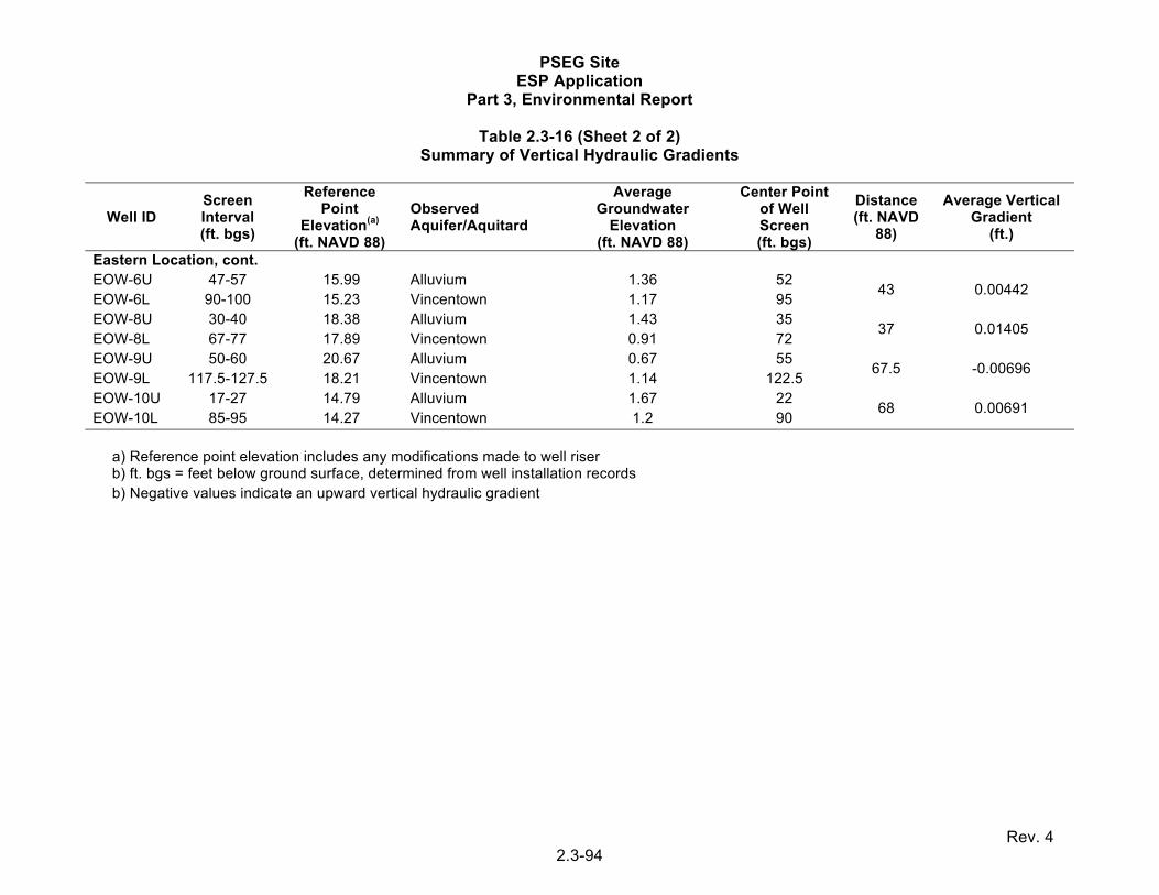
PSEG Site ESP Application
Part 3, Environmental Report
Rev. 4 2.3-94
Table 2.3-16 (Sheet 2 of 2) Summary of Vertical Hydraulic Gradients
Well ID Screen Interval (ft. bgs)
Reference Point
Elevation(a) (ft. NAVD 88)
Observed Aquifer/Aquitard
Average Groundwater
Elevation (ft. NAVD 88)
Center Point of Well Screen (ft. bgs)
Distance (ft. NAVD
88)
Average Vertical Gradient
(ft.)
Eastern Location, cont. EOW-6U 47-57 15.99 Alluvium 1.36 52
43 0.00442 EOW-6L 90-100 15.23 Vincentown 1.17 95 EOW-8U 30-40 18.38 Alluvium 1.43 35
37 0.01405 EOW-8L 67-77 17.89 Vincentown 0.91 72 EOW-9U 50-60 20.67 Alluvium 0.67 55
67.5 -0.00696 EOW-9L 117.5-127.5 18.21 Vincentown 1.14 122.5 EOW-10U 17-27 14.79 Alluvium 1.67 22
68 0.00691 EOW-10L 85-95 14.27 Vincentown 1.2 90
a) Reference point elevation includes any modifications made to well riser b) ft. bgs = feet below ground surface, determined from well installation records b) Negative values indicate an upward vertical hydraulic gradient

PSEG Site ESP Application
Part 3, Environmental Report
Rev. 4 2.3-95
Table 2.3-17 Summary of Average Hydraulic Conductivities
Well Formation Average Result
(ft./day)
Shallow NOW-1U Alluvium 8.0 NOW-2U Alluvium 8.0 NOW-3U Alluvium 0.3
NOW-4UB Alluvium 0.9 NOW-5U Hydraulic Fill 0.2 NOW-6U Alluvium 3.5 NOW-7U Vincentown 1.4 NOW-8U Alluvium 0.4
Deep NOW-1L Vincentown 4.5 NOW-2L Vincentown 3.6 NOW-3L Vincentown 1.4 NOW-4L Vincentown 10.7 NOW-5L Vincentown 1.7 NOW-6L Vincentown 6.2 NOW-7L Vincentown 2.4
NOW-8L Vincentown 0.3

PSEG Site ESP Application
Part 3, Environmental Report
Rev. 4 2.3-96
Table 2.3-18 Summary of Tidal Study Results
Measurement
Location Unit Barge Slip NOW-1L NOW-1U NOW-3L
NOW-3U
Max High Tide ft. NAVD 88 3.57 1.38
Tidal influence
not observed in
this observation
well
2.03 0.95
Min High Tide ft. NAVD 88 2.36 1.12 1.5 0.58
Max Low Tide ft. NAVD 88 -3.52 0.65 -0.75 0.41
Min Low Tide ft. NAVD 88 -2.27 0.86 -0.18 0.09
Average Tidal Shift ft. 5.85 0.49 2.26 0.56
Average Periodicity hr. 6.9 6.5 7 7.3
Average Phase Lag to Barge Slip min. N/A -66 -19
-62

PSEG Site ESP Application
Part 3, Environmental Report
Rev. 4 2.3-97
Table 2.3-19 Summary of Surface Water and Shallow Groundwater Elevations at Piezometers
Location ID 1/3
0/2
00
9
2/2
7/2
00
9
3/2
9/2
00
9
4/2
4/2
00
9
5/2
2/2
00
9
6/1
9/2
00
9
7/2
3/2
00
9
8/1
6/2
00
9
9/1
7/2
00
9
10
/16
/20
09
11
/11
/20
09
12
/10
/20
09
AS-01 - inside N/A NM N/A N/A 0.64 N/A NM N/A NM N/A N/A 1.12(a) AS-01 - outside N/A NM N/A N/A Dry N/A NM N/A NM N/A N/A -0.43(a) AS-02 - inside N/A NM N/A N/A -0.04 N/A 0.20 N/A 0.14 N/A N/A N/A AS-02 - outside N/A NM N/A N/A 2.52 N/A 1.75 N/A 1.59 N/A N/A N/A AS-03 - inside N/A NM N/A N/A -1.99 N/A -1.94 N/A -2.02 N/A N/A N/A AS-03 - outside N/A NM N/A N/A -0.23 N/A -0.15 N/A -2.02 N/A N/A N/A AS-04 - inside Frozen 4.19 4.04 4.49 4.34 4.09 3.55 3.02 3.73 3.55 3.88 4.32 AS-04 - outside 4.32 4.18 4.16 4.38 4.30 4.16 3.63 3.12 3.67 3.52 3.82 4.37 AS-05 - inside -0.41 0.54 0.17 0.58 -0.23 1.40 1.15 -3.63 1.63 1.21 1.27 1.46 AS-05 - outside 0.58 -0.09 -0.21 -0.13 -0.29 1.23 0.10 0.25 3.31 2.98 0.48 0.97 AS-06 - inside 0.80 0.93 1.14 0.83 0.86 1.74 Dry 0.73 3.09 3.23 1.95 1.87 AS-06 - outside 1.20 Dry Dry Dry Dry 2.51 1.09 Dry Dry Dry Dry Dry AS-08-pre-outside(b) 0.70 0.82 0.68 0.70 0.73 2.71 0.81 1.47 3.50 1.46 1.42 0.80 AS-08-pre-inside(b) 0.51 0.76 0.89 1.43 1.00 1.54 1.37 1.11 1.86 3.42 -2.17 2.27 AS-08-post-outside(b) 1.70 NM 2.25 1.87 1.26 Dry 0.76 1.48 3.25 NM Dry 0.77 AS-08-post-inside(b) 0.46 NM 1.43 1.21 1.04 Dry 1.34 2.80 1.90 NM Dry 2.00 AS-09 - inside Frozen 5.76 5.45 6.00 5.84 5.94 3.98 5.82 5.85 3.00 5.82 5.97 AS-09 - outside 6.24 5.87 5.89 5.97 5.81 5.93 5.37 5.83 5.83 5.75 5.80 6.17 AS-10 - inside 1.84 3.12 2.99 3.45 3.15 3.32 2.62 3.02 3.47 -0.06 3.42 3.70 AS-10 - outside 3.52 3.14 3.12 3.24 3.09 3.11 2.95 3.02 3.25 3.08 3.17 3.68 AS-11 - inside N/A NM N/A N/A 0.09 N/A 1.08 N/A 1.06 N/A N/A N/A AS-11 - outside N/A NM N/A N/A 0.70 N/A 2.11 N/A 2.04 N/A N/A N/A
Elevation data reported in feet NAVD 88 N/A = not applicable NM = could not be sampled / not measured a) Data measured on 1/07/10 b) The first and last reading of each event is conducted at PZ-8 so that a tidal change encompassing all water measurements can be evaluated

PSEG Site ESP Application
Part 3, Environmental Report
Rev. 4 2.3-98
Table 2.3-20 Water Withdrawal Estimates (Mgd) by Source in Delaware River Basin –
Lower Estuary and Bay Regions
Groundwater Surface Water 1995 2020 2040 1995 2020 2040
Total Withdrawals
Lower Estuary 50.5 60.5 86.9 3586.5 5056.7 6285.1
Delaware Bay 89.7 92.5 108.2 67.2 65.7 64.4
Consumptive Use
Lower Estuary 11.1 11.6 13.8 41.0 51.0 59.7
Delaware Bay 29.0 26.2 25.1 16.7 15.3 14.1
Reference 2.3-19

PSEG Site ESP Application
Part 3, Environmental Report
Rev. 4 2.3-99
Table 2.3-21 Peak Month Withdrawal and Consumptive
Uses by Sector for Dry Year (1995) and Wet Year (1996)
Sector Peak Withdrawal
(Mgd) Peak Consumptive Use
(Mgd) 1995 1996 1995 1996
Agriculture 186.5 93.5 167.9 84.1
Commercial/Industrial 13.9 12.0 1.4 1.2
Public Water Supply 1057.3 959.7 224.7 204.0
Domestic 89.5 6.3 18.4 1.3
Mining 113.5 103.5 17.0 15.5
Non-Agricultural Irrigation 17.8 8.3 16.0 7.5
Industrial 1174.1 893.9 55.6 46.5
Hydroelectric Power Generation 322.8 446.7 0.0 0.0
Thermoelectric Power Generation
5973.4 6272.9 85.4 82.1
Other 19.6 9.4 0.5 0.2
Totals 8968.4 8806.2 587.1 442.4
Reference 2.3-19

PSEG Site ESP Application
Part 3, Environmental Report
Rev. 4 2.3-100
Table 2.3-22 Delaware River Basin Water Supply Reservoirs
Reservoir
Purpose(a) Storage (Million Gallons) Location
WS/WSA/P Flood Loss
Reduction
Water Supply Penn Forest WS 6510 Wild Creek; Carbon County, PA Wild Creek WS 3910 Wild Creek; Carbon County, PA Still Creek WS 2701 Still Creek; Schuylkill County, PA Ontelaunee WS 3793 Martins Creek; Berks County, PA Green Lane WS 4376 Perkiomen Creek; Montgomery
County, PA Geist WS 3512 Crum Creek; Delaware County, PA Edgar Hoopes WS 2199 Tributary to Red Clay Creek; New
Castle County, DE Union Lake WS 3177 Maurice River; Cumberland County,
NJ Hopatcong WS(b) 5995 Musconetcong River; Sussex, Morris
County, NJ Nockamixon WS(c) 11,990 Tohickon Creek; Bucks County, PA
New York City Reservoirs Cannonsville WS, WSA 98,400 West Branch Delaware River;
Delaware County, NY Neversink WS, WSA 35,581 Neversink River, Sullivan County, NY Pepacton WS, WSA 147,926 East Branch Delaware River;
Delaware County, NY Hydroelectric Power Generation
Lake Wallenpaupack
P 29,813 Wallenpaupack Creek; Wayne County, PA
Mongaup System
P 15,314 Mongaup River, Sullivan County, NY
Multipurpose or Flood Loss Reduction Prompton FL None 6614 West Branch Lackawaxen River;
Wayne County, PA Beltzville WSA, FL 12,978 8797 Pohopoco Creek; Carbon County, PAMarsh Creek WS, WSA, FL(d) 4040 1160 Marsh Creek; Chester County, PA Chambers Lake WS, WSA 383 None Birch Run; Chester County, PA Blue Marsh WSA, FL 4757 10,554 Tulpehocken Creek; Berks County,
PA Lake Galena WS, FL 1629 1127 North Branch Neshaminy Creek;
Bucks County, PA Francis E. Walter
FL None 35,190 Lehigh River; Luzerne, Carbon County, PA
Jadwin FL None 7983 Dyberry Creek; Wayne County, PA Merrill Creek WSA 15,640 None Merrill Creek; Hunterdon County, NJ Total Storage 414,624
a) WS – Water Supply, WSA – water supply primarily for flow augmentation, P – hydroelectric power generation, FL – Flood Loss b) Emergency use only c) Used for flow maintenance during emergencies d) Used for flow maintenance in Brandywine Creek Reference 2.3-19

PSEG Site ESP Application
Part 3, Environmental Report
Rev. 4 2.3-101
Table 2.3-23 Water Withdrawals and Consumptive Use by Power Generation Facilities
(1995 Average Demands)
Site Name Withdrawal
(Mgd)
Consumptive Use (Mgd)
Actual EIF
Adjusted Exelon – Limerick Unit 35.6 27.1 27.1 PSEG – Salem and Hope Creek 2473.4 15.3 2.3 Exelon – Eddystone Unit 716.1 4.3 3.6 Connective – Hay Road 537.8 4.1 2.4 PSEG – Mercer Station 461.4 2.9 2.9 Wheelabrator Gloucester County, LP 16.3 1.6 1.6 Reliant Energy – Gilbert (1-3) 15.1 1.5 1.5 Reliant Energy – Portland 219.7 1.5 1.5 Logan Generating County, LP 1.4 1.4 1.0 PP&L – Martins Creek 58.3 1.4 1.4 Exelon – Cromby 223.0 1.3 1.3 Reliant Energy – Titus (surface water withdrawal)
12.9 1.1 1.1
Wheelabrator Frackville Energy County Inc.
1.7 1.1 1.1
Panther Creek Partners 1.0 1.0 1.0 Reliant Energy – Yards Creek 7.2 0.7 0.7 PSEG – Burlington Station 85.5 0.6 0.6 Northampton Generating- Lehigh River 0.6 0.6 0.6 Exelon – Delaware Unit 75.4 0.5 0.5 Conectiv – Deepwater Station 103.3 0.4 0.2 Chambers Cogen - Carneys Point 3.1 0.3 0.2 Exelon – Schuylkill Unit 36.8 0.3 0.3 Warren Energy Resource County, LP 0.2 0.1 0.1 Peco Energy Co – Richmond 1.3 0.1 0.1 Reliant Energy Gilbert (8) 1.2 0.1 0.1 Northeastern Power – Silverbrook Mine 0.1 0.1 0.1 Pedricktown Cogen/Conectiv 0.5 0.0 0.0 Reliant Energy – Titus (Wells) 0.2 0.0 0.0 Tractebel Electricity & Gas 0.1 0.0 0.0 Reliant Energy – Gilbert 0.0 0.0 0.0 Great Bear Hydropower, Inc. 145.4 0.0 0.0 PP&L – Wallenpaupack 189.0 0.0 0.0 Total 5423.6 69.4 53.3 EIF – Equivalent Impact Factor Reference 2.3-19
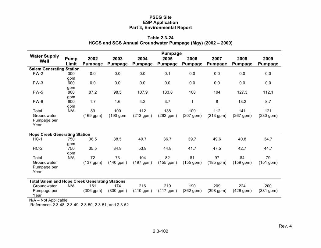
PSEG Site ESP Application
Part 3, Environmental Report
Rev. 4 2.3-102
Table 2.3-24 HCGS and SGS Annual Groundwater Pumpage (Mgy) (2002 – 2009)
Water Supply Well
PumpagePump Limit
2002 Pumpage
2003 Pumpage
2004 Pumpage
2005 Pumpage
2006 Pumpage
2007 Pumpage
2008 Pumpage
2009 Pumpage
Salem Generating Station PW-2 300
gpm 0.0 0.0 0.0 0.1 0.0 0.0 0.0 0.0
PW-3 600 gpm
0.0 0.0 0.0 0.0 0.0 0.0 0.0 0.0
PW-5 800 gpm
87.2 98.5 107.9 133.8 108 104 127.3 112.1
PW-6 600 gpm
1.7 1.6 4.2 3.7 1 8 13.2 8.7
Total Groundwater Pumpage per Year
N/A 89 (169 gpm)
100 (190 gpm
112 (213 gpm)
138 (262 gpm)
109 (207 gpm)
112 (213 gpm)
141 (267 gpm)
121 (230 gpm)
Hope Creek Generating Station
HC-1 750 gpm
36.5 38.5 49.7 36.7 39.7 49.6 40.8 34.7
HC-2 750 gpm
35.5 34.9 53.9 44.8 41.7 47.5 42.7 44.7
Total Groundwater Pumpage per Year
N/A 72 (137 gpm)
73 (140 gpm)
104 (197 gpm)
82 (155 gpm)
81 (155 gpm)
97 (185 gpm)
84 (159 gpm)
79 (151 gpm)
Total Salem and Hope Creek Generating Stations
Groundwater Pumpage per Year
N/A 161 (306 gpm)
174 (330 gpm)
216 (410 gpm)
219 (417 gpm)
190 (362 gpm)
209 (398 gpm)
224 (426 gpm)
200 (381 gpm)
N/A – Not Applicable References 2.3-48, 2.3-49, 2.3-50, 2.3-51, and 2.3-52

PSEG Site ESP Application
Part 3, Environmental Report
Rev. 4 2.3-103
Table 2.3-25 (Sheet 1 of 2) Summary of Analytical Data – Artificial Pond Locations (AS-8)
Chem Class Parameter Units Detects Samples Min DL(a)
Max DL(a)
Min Max Mean(b)
Metals (Total) Calcium mg/L 4 4 78.6 115 99 Lead mg/L 4 4 0.0025 0.0066 0.0048
Magnesium mg/L 4 4 192 288 250 Potassium mg/L 0 4 62.4 91 78 Sodium mg/L 4 4 1600 2490 2100 Zinc mg/L 4 4 0.0184 0.0321 0.026 Mercury mg/L 0 4 0.0002 0.0002Inorganics Alkalinity, Total mg/L 4 4 60.8 65.7 63 Ammonia mg/L 4 4 0.058 0.31 0.13
Biochemical Oxygen Demand mg/L 4 4 0.84 5.2 2.4
Chemical Oxygen Demand mg/L 4 4 46.9 74.8 67
Chloride mg/L 4 4 2940 5070 4200 Cyanide, Total mg/L 1 4 0.03 0.03 0.0425 0.0425 Hardness as CaCO3 mg/L 4 4 987 1470 1300 Nitrate as N mg/L 3 4 0.1 0.1 0.29 0.59 0.32 Nitrate+Nitrite as N mg/L 3 4 1 1 0.7 2.2 1.3 Nitrite as N mg/L 2 4 2.5 5 0.15 1.2 1.3 Nitrogen, Total Kjeldahl mg/L 4 4 0.36 0.64 0.52 Orthophosphate mg/L 0 4 0.1 0.5 Phosphorus, Total as P mg/L 4 4 0.16 0.23 0.19 Sulfate mg/L 4 4 365 638 500 Total Dissolved Solids mg/L 4 4 5340 7780 6800 Total Suspended Solids mg/L 4 4 85 207 150
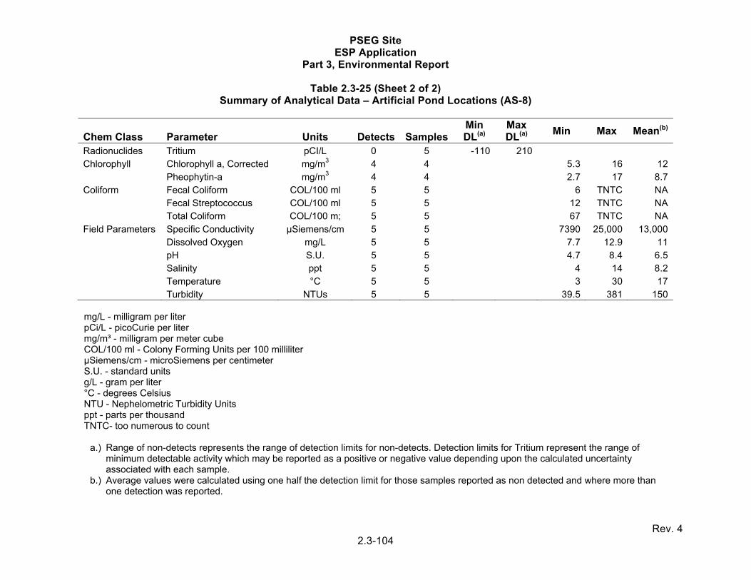
PSEG Site ESP Application
Part 3, Environmental Report
Rev. 4 2.3-104
Table 2.3-25 (Sheet 2 of 2) Summary of Analytical Data – Artificial Pond Locations (AS-8)
Chem Class Parameter Units Detects Samples Min DL(a)
Max DL(a)
Min Max Mean(b)
Radionuclides Tritium pCI/L 0 5 -110 210Chlorophyll Chlorophyll a, Corrected mg/m3 4 4 5.3 16 12 Pheophytin-a mg/m3 4 4 2.7 17 8.7Coliform Fecal Coliform COL/100 ml 5 5 6 TNTC NA Fecal Streptococcus COL/100 ml 5 5 12 TNTC NA Total Coliform COL/100 m; 5 5 67 TNTC NAField Parameters Specific Conductivity µSiemens/cm 5 5 7390 25,000 13,000 Dissolved Oxygen mg/L 5 5 7.7 12.9 11 pH S.U. 5 5 4.7 8.4 6.5 Salinity ppt 5 5 4 14 8.2 Temperature °C 5 5 3 30 17 Turbidity NTUs 5 5 39.5 381 150
mg/L - milligram per liter pCi/L - picoCurie per liter mg/m³ - milligram per meter cube COL/100 ml - Colony Forming Units per 100 milliliter µSiemens/cm - microSiemens per centimeter S.U. - standard units g/L - gram per liter °C - degrees Celsius NTU - Nephelometric Turbidity Units ppt - parts per thousand TNTC- too numerous to count
a.) Range of non-detects represents the range of detection limits for non-detects. Detection limits for Tritium represent the range of minimum detectable activity which may be reported as a positive or negative value depending upon the calculated uncertainty associated with each sample.
b.) Average values were calculated using one half the detection limit for those samples reported as non detected and where more than one detection was reported.

PSEG Site ESP Application
Part 3, Environmental Report
Rev. 4 2.3-105
Table 2.3-26 (Sheet 1 of 2) Summary of Analytical Data – Artificial Pond Locations (AS-4, AS-9, AS-14)
Chem Class Parameter Units Detects Samples Min DL(a)
Max DL(a)
Min Max Mean(b)
Metals (Total) Calcium mg/L 12 12 23.3 75.3 56 Lead mg/L 8 12 0.0025 0.005 0.00057 0.0099 0.0027
Magnesium mg/L 12 12 23.3 94.2 61 Potassium mg/L 12 12 16.2 31.1 23 Sodium mg/L 12 12 243 496 410 Zinc mg/L 8 12 0.025 0.05 0.0067 0.0463 0.017 Mercury mg/L 0 12 0.0002 0.0002Inorganics Alkalinity, Total mg/L 12 12 115 304 0.18 Ammonia mg/L 12 12 0.058 0.45 7.6
Biochemical Oxygen Demand mg/L 12 12 2.9 26.2 69
Chemical Oxygen Demand mg/L 12 12 23.9 158 660
Chloride mg/L 12 12 314 951 390 Cyanide, Total mg/L 1 12 0.01 0.01 0.0043 0.0043 Hardness as CaCO3 mg/L 12 12 213 572 0.061 Nitrate as N mg/L 1 12 0.1 0.1 0.18 0.18 Nitrate+Nitrite as N mg/L 5 12 0.5 1 0.12 1.1 0.38 Nitrite as N mg/L 6 12 0.5 1 0.055 0.6 2.4 Nitrogen, Total Kjeldahl mg/L 12 12 0.8 5.9 0.096 Orthophosphate mg/L 1 12 0.1 0.1 0.15 0.15 Phosphorus, Total as P mg/L 12 12 0.075 0.59 180 Sulfate mg/L 12 12 33.3 530 1500 Total Dissolved Solids mg/L 12 12 887 2060 49 Total Suspended Solids mg/L 12 12 3.7 314 91

PSEG Site ESP Application
Part 3, Environmental Report
Rev. 4 2.3-106
Table 2.3-26 (Sheet 2 of 2) Summary of Analytical Data – Artificial Pond Locations (AS-4, AS-9, AS-14)
Chem Class Parameter Units Detects Samples Min DL(a)
Max DL(a)
Min Max Mean(b)
Radionuclides Tritium pCI/L 1 12 70 270 270 270Chlorophyll Chlorophyll a, Corrected mg/m3 12 12 14 178 52 Pheophytin-a mg/m3 10 12 1 1 8 114 31Coliform Fecal Coliform COL/100 ml 11 12 1 1 1 90 32 Fecal Streptococcus COL/100 ml 12 12 2 72 36 Total Coliform COL/100 m; 12 12 13 TNTC NAField Parameters Specific Conductivity µSiemens/cm 13 13 1170 28,400 6378 Dissolved Oxygen mg/L 13 13 5 1198 101 pH S.U. 13 13 5.93 8.1 7.29 Salinity ppt 12 13 1 1 1 2 1.1 Temperature °C 13 13 3 29 19.38 Turbidity NTUs 13 13 10.1 712 123.72
mg/L - milligram per liter pCi/L - picoCurie per liter mg/m³ - milligram per meter cube COL/100 ml - Colony Forming Units per 100 milliliter µSiemens/cm - microSiemens per centimeter S.U. - standard units g/L - gram per liter °C - degrees Celsius NTU - Nephelometric Turbidity Units ppt - parts per thousand TNTC- too numerous to count
a) Range of non-detects represents the range of detection limits for non-detects. Detection limits for Tritium represent the range of minimum detectable activity which may be reported as a positive or negative value depending upon the calculated uncertainty associated with each sample.
b) Average values were calculated using one half the detection limit for those samples reported as non detected and where more than one detection was reported.
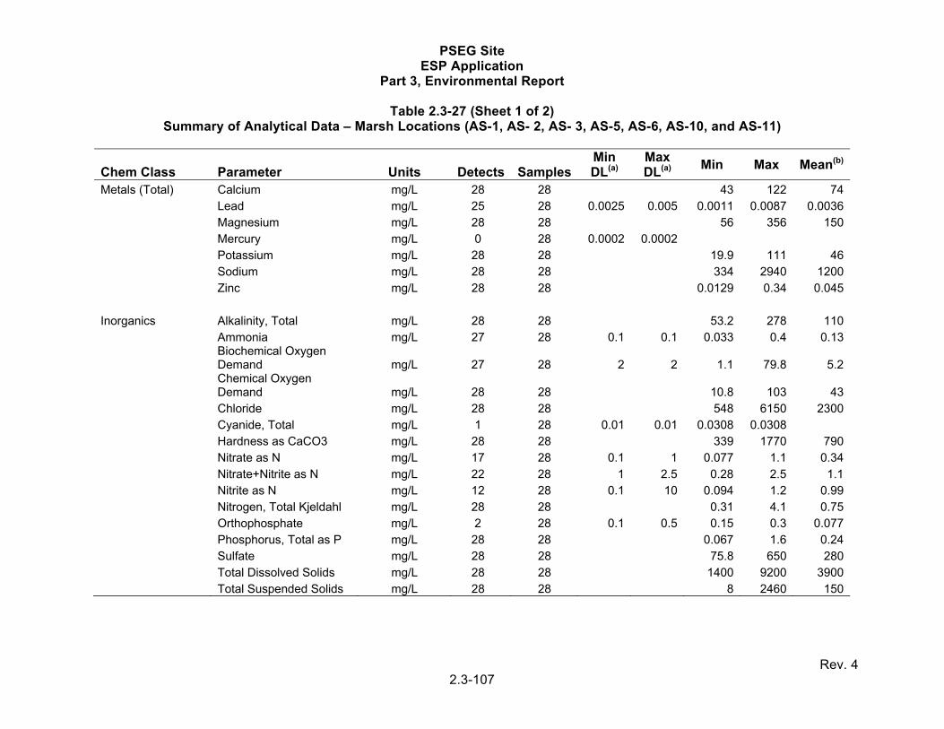
PSEG Site ESP Application
Part 3, Environmental Report
Rev. 4 2.3-107
Table 2.3-27 (Sheet 1 of 2) Summary of Analytical Data – Marsh Locations (AS-1, AS- 2, AS- 3, AS-5, AS-6, AS-10, and AS-11)
Chem Class Parameter Units Detects Samples Min DL(a)
Max DL(a)
Min Max Mean(b)
Metals (Total) Calcium mg/L 28 28 43 122 74 Lead mg/L 25 28 0.0025 0.005 0.0011 0.0087 0.0036 Magnesium mg/L 28 28 56 356 150 Mercury mg/L 0 28 0.0002 0.0002 Potassium mg/L 28 28 19.9 111 46 Sodium mg/L 28 28 334 2940 1200 Zinc mg/L 28 28 0.0129 0.34 0.045 Inorganics Alkalinity, Total mg/L 28 28 53.2 278 110 Ammonia mg/L 27 28 0.1 0.1 0.033 0.4 0.13
Biochemical Oxygen Demand mg/L 27 28 2 2 1.1 79.8 5.2
Chemical Oxygen Demand mg/L 28 28 10.8 103 43
Chloride mg/L 28 28 548 6150 2300 Cyanide, Total mg/L 1 28 0.01 0.01 0.0308 0.0308 Hardness as CaCO3 mg/L 28 28 339 1770 790 Nitrate as N mg/L 17 28 0.1 1 0.077 1.1 0.34 Nitrate+Nitrite as N mg/L 22 28 1 2.5 0.28 2.5 1.1 Nitrite as N mg/L 12 28 0.1 10 0.094 1.2 0.99 Nitrogen, Total Kjeldahl mg/L 28 28 0.31 4.1 0.75 Orthophosphate mg/L 2 28 0.1 0.5 0.15 0.3 0.077 Phosphorus, Total as P mg/L 28 28 0.067 1.6 0.24 Sulfate mg/L 28 28 75.8 650 280 Total Dissolved Solids mg/L 28 28 1400 9200 3900 Total Suspended Solids mg/L 28 28 8 2460 150

PSEG Site ESP Application
Part 3, Environmental Report
Rev. 4 2.3-108
Table 2.3-27 (Sheet 2 of 2) Summary of Analytical Data – Marsh Locations (AS-1, AS- 2, AS- 3, AS-5, AS-6, AS-10, and AS-11)
Chem Class Parameter Units Detects Samples Min DL(a)
Max DL(a)
Min Max Mean(b)
Radionuclides Tritium PCI/L 1 28 -70 310 290 290Chlorophyll Chlorophyll a, Corrected mg/m3 28 28 2.2 243 21 Pheophytin-a mg/m3 18 28 1 1 1.4 100 7Coliform Fecal Coliform COL/100 ML 27 28 1 1 1 TNTC NA Fecal Streptococcus COL/100 ML 28 28 5 TNTC NA Total Coliform COL/100 ML 27 28 1 1 132 TNTC NAField Parameters Specific Conductivity µSiemens/cm 29 29 1360 93,500 9477 Dissolved Oxygen mg/L 29 29 4.6 13.3 8.7 pH S.U. 29 29 4.7 8.6 6.8 Salinity ppt 29 29 1 9 3.4 Temperature °C 28 29 1 1 2 27 17.5 Turbidity NTUs 29 29 26.2 449 116.7
mg/L - milligram per liter pCi/L - picoCurie per liter mg/m³ - milligram per meter cube COL/100 ML - Colony Forming Units per 100 milliliter µSiemens/cm - microSiemens per centimeter S.U. - standard units g/L - gram per liter °C - degrees Celsius NTU - Nephelometric Turbidity Units ppt - parts per thousand TNTC- too numerous to count
a) Range of non-detects represents the range of detection limits for non-detects. Detection limits for Tritium represent the range of minimum detectable activity which may be reported as a positive or negative value depending upon the calculated uncertainty associated with each sample.
b) Average values were calculated using one half the detection limit for those samples reported as non detected and where more than one detection was reported.

PSEG Site ESP Application
Part 3, Environmental Report
Rev. 4 2.3-109
Table 2.3-28 (Sheet 1 of 2) Summary of Analytical Data for Upper (Alluvium) New Plant Observation Well Locations
Chem Class Parameter Units Detects Samples Min DL(a)
Max DL(a)
Min Max Mean(b)
Metals (Total) Calcium mg/L 32 32 89.4 365 170 Iron mg/L 32 32 3.66 57.9 33 Lead mg/L 13 32 0.0025 0.005 0.00099 0.0031 0.0021 Magnesium mg/L 32 32 84.9 328 240 Mercury mg/L 0 32 0.0002 0.0002 Potassium mg/L 32 32 19.4 73 47 Sodium mg/L 32 32 1110 2660 1600Metals (Dissolved) Silica crystalline quartz mg/L 32 32 14.4 55.9 33Inorganics Alkalinity, Total mg/L 32 32 530 1390 1100 Ammonia mg/L 32 32 2.5 58.1 33 Bicarbonate as HCO3 mg/L 32 32 530 1390 1100
Biochemical Oxygen Demand mg/L 28 32 2 20 1.7 256 39
Carbon Dioxide mg/L 32 32 36 150 95
Chemical Oxygen Demand mg/L 32 32 33.9 565 170
Chloride mg/L 32 32 1670 4160 2900 Hardness as CaCO3 mg/L 32 32 1180 1940 1400 Nitrate as N mg/L 6 32 0.1 2 0.11 0.76 0.21 Nitrate+Nitrite as N mg/L 4 32 1 5 1.2 1.2 1.8 Nitrite as N mg/L 7 32 1 5 0.23 0.48 1.8 Nitrogen, Total Kjeldahl mg/L 29 32 0.1 0.5 0.6 17.3 6.5 Orthophosphate mg/L 0 32 0.1 0.1 Phosphorus, Total as P mg/L 32 32 0.035 5.6 3 Sulfate mg/L 12 32 1 1 0.69 89.4 13 Total Dissolved Solids mg/L 32 32 4150 7030 5500 Total Suspended Solids mg/L 32 32 19 216 130

PSEG Site ESP Application
Part 3, Environmental Report
Rev. 4 2.3-110
Table 2.3-28 (Sheet 2 of 2) Summary of Analytical Data for Upper (Alluvium) New Plant Observation Well Locations
Chem Class Parameter Units Detects Samples Min DL(a)
Max DL(a)
Min Max Mean(b)
Radionuclides Tritium pCI/L 0 32 -130 220 11Coliform (CFU) Fecal Coliform COL/100 ml 1 32 1 1 2 2 0.55 Fecal Streptococcus COL/100 ml 9 32 1 1 1 54 5.9 Total Coliform COL/100 ml 11 32 1 1 8 TNTC NAField Parameters Specific Conductivity µSiemens/cm 35 35 4160 95000 19000 Dissolved Oxygen mg/L 10 35 0.1 0.1 0.7 3.6 0.53 Eh mv 35 35 -240 15 -150 pH S.U. 35 35 6.5 10.4 7.0 Salinity ppt 35 35 2 9 5.4 Temperature °C 35 35 12 21 16 Turbidity NTUs 34 35 0.1 0.1 2.5 604 94
mg/L - milligram per liter pCi/L - picoCurie per liter mg/m³ - milligram per meter cube COL/100 ML - Colony Forming Units per 100 milliliter µSiemens/cm - microSiemens per centimeter S.U. - standard units g/L - gram per liter °C - degrees Celsius NTU - Nephelometric Turbidity Units ppt - parts per thousand TNTC- too numerous to count
a) Range of non-detects represents the range of detection limits for non-detects. Detection limits for Tritium represent the range of minimum detectable activity which may be reported as a positive or negative value depending upon the calculated uncertainty associated with each sample.
b) Average values were calculated using one half the detection limit for those samples reported as non detected and where more than one detection was reported.

PSEG Site ESP Application
Part 3, Environmental Report
Rev. 4 2.3-111
Table 2.3-29 (Sheet 1 of 2) Summary of Analytical Data for Upper (Alluvium) Eastern Observation Well Locations
Chem Class Parameter Units Detects Samples Min DL(a)
Max DL(a)
Min Max Mean(b)
Metals (Total) Calcium mg/L 32 32 81.7 193 130 Iron mg/L 32 32 17 75.3 47 Lead mg/L 10 32 0.005 0.005 0.0014 0.02 0.0041 Magnesium mg/L 32 32 97.8 382 270 Mercury mg/L 1 32 0.0002 0.0002 0.00014 0.00014 Potassium mg/L 32 32 27.3 87.3 69 Sodium mg/L 32 32 194 2710 1900Metals (Dissolved) Silica crystalline quartz mg/L 32 32 8.14 47.8 26Inorganics Alkalinity, Total mg/L 32 32 389 1310 960 Ammonia mg/L 32 32 9.5 49.9 33 Bicarbonate as HCO3 mg/L 32 32 389 1310 960
Biochemical Oxygen Demand mg/L 32 32 1.6 237 31
Carbon Dioxide mg/L 32 32 34 140 79 Chemical Oxygen Demand mg/L 31 32 36 36 44.5 482 200 Chloride mg/L 32 32 61.5 5280 3500 Hardness as CaCO3 mg/L 32 32 720 1890 1500 Nitrate as N mg/L 8 32 0.1 2 0.061 0.11 0.11 Nitrate+Nitrite as N mg/L 3 32 0.1 5 1.2 1.2 1.7 Nitrite as N mg/L 7 32 0.1 5 0.2 0.48 1.7 Nitrogen, Total Kjeldahl mg/L 29 32 0.5 2.6 2 51.4 8.4 Orthophosphate mg/L 0 32 0.1 0.1 Phosphorus, Total as P mg/L 32 32 0.85 4.9 2.7 Sulfate mg/L 7 32 0.1 1 0.98 791 92 Total Dissolved Solids mg/L 32 32 1500 8270 6200 Total Suspended Solids mg/L 32 32 74 413 170

PSEG Site ESP Application
Part 3, Environmental Report
Rev. 4 2.3-112
Table 2.3-29 (Sheet 2 of 2) Summary of Analytical Data for Upper (Alluvium) Eastern Observation Well Locations
Chem Class Parameter Units Detects Samples Min DL(a)
Max DL(a)
Min Max Mean(b)
Radionuclides Tritium pCI/L 2 32 -180 180 340 710 38Coliform (CFU) Fecal Coliform COL/100 ml 1 32 1 1 29 29 Fecal Streptococcus COL/100 ml 5 32 1 4 1 TNTC NA Total Coliform COL/100 ml 18 32 1 1 1 TNTC NAField Parameters Specific Conductivity µSiemens/cm 32 32 2090 99,900 20,000 Dissolved Oxygen mg/L 18 32 0.1 0.1 0.1 6.5 0.76 Eh mv 32 32 -250 -1 -160 pH S.U. 32 32 6.4 10.4 7.1 Salinity ppt 32 32 1 40 8.1 Temperature °C 32 32 12 19 15 Turbidity NTUs 27 32 0.1 0.1 0.3 999 140 mg/L - milligram per liter pCi/L - picoCurie per liter mg/m³ - milligram per meter cube COL/100 ML - Colony Forming Units per 100 milliliter µSiemens/cm - microSiemens per centimeter S.U. - standard units g/L - gram per liter °C - degrees Celsius NTU - Nephelometric Turbidity Units ppt - parts per thousand TNTC- too numerous to count
a) Range of non-detects represents the range of detection limits for non-detects. Detection limits for Tritium represent the range of minimum detectable activity which may be reported as a positive or negative value depending upon the calculated uncertainty associated with each sample.
b) Average values were calculated using one half the detection limit for those samples reported as non detected and where more than one detection was reported.
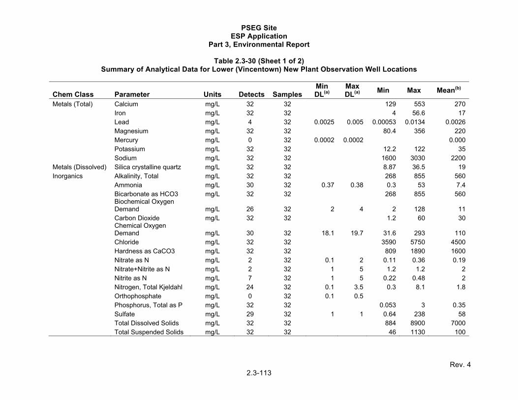
PSEG Site ESP Application
Part 3, Environmental Report
Rev. 4 2.3-113
Table 2.3-30 (Sheet 1 of 2) Summary of Analytical Data for Lower (Vincentown) New Plant Observation Well Locations
Chem Class Parameter Units Detects Samples Min DL(a)
Max DL(a)
Min Max Mean(b)
Metals (Total) Calcium mg/L 32 32 129 553 270 Iron mg/L 32 32 4 56.6 17 Lead mg/L 4 32 0.0025 0.005 0.00053 0.0134 0.0026 Magnesium mg/L 32 32 80.4 356 220 Mercury mg/L 0 32 0.0002 0.0002 0.000 Potassium mg/L 32 32 12.2 122 35 Sodium mg/L 32 32 1600 3030 2200Metals (Dissolved) Silica crystalline quartz mg/L 32 32 8.87 36.5 19Inorganics Alkalinity, Total mg/L 32 32 268 855 560 Ammonia mg/L 30 32 0.37 0.38 0.3 53 7.4 Bicarbonate as HCO3 mg/L 32 32 268 855 560
Biochemical Oxygen Demand mg/L 26 32 2 4 2 128 11
Carbon Dioxide mg/L 32 32 1.2 60 30
Chemical Oxygen Demand mg/L 30 32 18.1 19.7 31.6 293 110
Chloride mg/L 32 32 3590 5750 4500 Hardness as CaCO3 mg/L 32 32 809 1890 1600 Nitrate as N mg/L 2 32 0.1 2 0.11 0.36 0.19 Nitrate+Nitrite as N mg/L 2 32 1 5 1.2 1.2 2 Nitrite as N mg/L 7 32 1 5 0.22 0.48 2 Nitrogen, Total Kjeldahl mg/L 24 32 0.1 3.5 0.3 8.1 1.8 Orthophosphate mg/L 0 32 0.1 0.5 Phosphorus, Total as P mg/L 32 32 0.053 3 0.35 Sulfate mg/L 29 32 1 1 0.64 238 58 Total Dissolved Solids mg/L 32 32 884 8900 7000 Total Suspended Solids mg/L 32 32 46 1130 100

PSEG Site ESP Application
Part 3, Environmental Report
Rev. 4 2.3-114
Table 2.3-30 (Sheet 2 of 2) Summary of Analytical Data for Lower (Vincentown) New Plant Observation Well Locations
Chem Class Parameter Units Detects Samples Min DL(a)
Max DL(a)
Min Max Mean(b)
Radionuclides Tritium pCI/L 0 32 -110 160Coliform (CFU) Fecal Coliform COL/100 ml 2 32 1 1 1 1 0.53 Fecal Streptococcus COL/100 ml 4 32 1 1 1 38 2.1 Total Coliform COL/100 ml 15 32 1 1 4 TNTC NAField Parameters Specific Conductivity µSiemens/cm 35 35 8070 83,600 16,000 Dissolved Oxygen mg/L 16 35 0.1 0.1 0.4 7 0.69 Eh mv 35 35 -390 -1 -160 pH S.U. 35 35 6.7 10.6 7.4 Salinity ppt 35 35 4 14 8.2 Temperature °C 35 35 11 19 15 Turbidity NTUs 27 35 0.1 0.1 0.2 637 59 mg/L - milligram per liter pCi/L - picoCurie per liter mg/m³ - milligram per meter cube COL/100 ML - Colony Forming Units per 100 milliliter µSiemens/cm - microSiemens per centimeter S.U. - standard units g/L - gram per liter °C - degrees Celsius NTU - Nephelometric Turbidity Units ppt - parts per thousand TNTC- too numerous to count
a) Range of non-detects represents the range of detection limits for non-detects. Detection limits for Tritium represent the range of minimum detectable activity which may be reported as a positive or negative value depending upon the calculated uncertainty associated with each sample.
b) Average values were calculated using one half the detection limit for those samples reported as non detected and where more than one detection was reported.

PSEG Site ESP Application
Part 3, Environmental Report
Rev. 4 2.3-115
Table 2.3-31 (Sheet 1 of 2) Summary of Analytical Data for Lower (Vincentown) Eastern Observation Well Locations
Chem Class Parameter Units Detects Samples Min DL(a)
Max DL(a)
Min Max Mean(b)
Metals (Total) Calcium mg/L 32 32 169 757 440 Iron mg/L 32 32 1.6 86.6 31 Lead mg/L 1 32 0.0025 0.005 0.0028 0.0028 0.002 Magnesium mg/L 32 32 116 417 260 Mercury mg/L 0 32 0.0002 0.0002 0.000 Potassium mg/L 32 32 7.64 67.9 37 Sodium mg/L 32 32 2130 3120 2700Metals (Dissolved) Silica crystalline quartz mg/L 32 32 14 31.9 26Inorganics Alkalinity, Total mg/L 32 32 326 918 600 Ammonia mg/L 29 32 0.76 0.99 0.83 16.8 4.7 Bicarbonate as HCO3 mg/L 32 32 326 918 600
Biochemical Oxygen Demand mg/L 28 32 2 4 0.74 139 13
Carbon Dioxide mg/L 32 32 23 100 61
Chemical Oxygen Demand mg/L 32 32 28.3 325 140
Chloride mg/L 32 32 4330 6730 5600 Hardness as CaCO3 mg/L 32 32 1930 2420 2200 Nitrate as N mg/L 13 32 0.1 2 0.11 0.11 0.25 Nitrate+Nitrite as N mg/L 1 32 1 5 1.2 1.2 Nitrite as N mg/L 5 32 1 5 0.44 0.46 2 Nitrogen, Total Kjeldahl mg/L 24 32 0.42 2.9 0.46 4.5 1.3 Orthophosphate mg/L 0 32 0.1 0.1 Phosphorus, Total as P mg/L 32 32 0.09 2.3 0.69 Sulfate mg/L 32 32 12.6 281 97 Total Dissolved Solids mg/L 32 32 7470 10,000 9000 Total Suspended Solids mg/L 32 32 20.7 269 100

PSEG Site ESP Application
Part 3, Environmental Report
Rev. 4 2.3-116
Table 2.3-31 (Sheet 2 of 2) Summary of Analytical Data for Lower (Vincentown) Eastern Observation Well Locations
Chem Class Parameter Units Detects SamplesMin DL(a)
Max DL(a)
Min Max Mean(b)
Radionuclides Tritium pCI/L 0 32 -120 260 Coliform (CFU) Fecal Coliform COL/100 ml 0 32 1 1 Fecal Streptococcus COL/100 ml 1 32 1 1 2 2 Total Coliform COL/100 ml 20 32 1 1 1 TNTC NAField Parameters Specific Conductivity µSiemens/cm 33 33 12,900 79,800 20,000 Dissolved Oxygen mg/L 10 33 0.1 0.1 0.11 4.6 0.5 Eh mv 33 33 -310 -5 -140 pH S.U. 33 33 6.2 9.9 6.9 Salinity ppt 33 33 4 23 11 Temperature °C 33 33 9 17 15 Turbidity NTUs 16 33 0.1 0.1 2.4 179 24 mg/L - milligram per liter pCi/L - picoCurie per liter mg/m³ - milligram per meter cube COL/100 ML - Colony Forming Units per 100 milliliter µSiemens/cm - microSiemens per centimeter S.U. - standard units g/L - gram per liter °C - degrees Celsius NTU - Nephelometric Turbidity Units ppt - parts per thousand TNTC- too numerous to count
a) Range of non-detects represents the range of detection limits for non-detects. Detection limits for Tritium represent the range of minimum detectable activity which may be reported as a positive or negative value depending upon the calculated uncertainty associated with each sample.
b) Average values were calculated using one half the detection limit for those samples reported as non detected and where more than one detection was reported.

PSEG Site ESP Application
Part 3, Environmental Report
Rev. 4 2.4-1
2.4 ECOLOGY This section provides a description and characterization of the terrestrial and aquatic ecosystems potentially affected by the construction and operation of the new plant at the PSEG Site. Consultations with the NJDEP (Reference 2.4-142), DE Department of Natural Resources and Environmental Control (DNREC) (Reference 2.4-38), and U.S. Fish and Wildlife Service (USFWS) were initiated for information regarding ecological resources in the vicinity of the PSEG Site. This consultation process was used to obtain agency input regarding threatened and endangered species, sensitive habitats, commercial and recreational species, and other ecological characteristics for the site and vicinity. 2.4.1 TERRESTRIAL ECOLOGY This subsection presents the terrestrial ecology of the PSEG Site and the 6-mi. vicinity based on historical data collected in support of HCGS and SGS licensing, recorded information provided by resource agencies, and supplemental field surveys conducted in 2009 - 2010. Historic field studies include plant and animal surveys conducted on and in the vicinity of the PSEG Site. These historic field studies include:
Studies conducted on the terrestrial ecology of Artificial Island and vicinity including birds, mammals, herpetofauna (reptiles and amphibians), and vegetation (References 2.4-24, 2.4-87, 2.4-220, 2.4-221, 2.4-222).
Wetland delineation studies documenting wetlands on and near the PSEG Site (References 2.4-1).
Annual biological monitoring reports by PSEG (1995 to 2009) documenting vegetation and fish as part of the PSEG Estuary Enhancement Program (EEP) both on-site and in the PSEG Site vicinity (References 2.4-153 through 2.4-157 and 2.4-159 through 2.4-166).
Terrestrial ecological studies conducted for the PSEG access road widening project in the early 1980s, documenting birds, mammals, vegetation and fish (Reference 2.4-158).
Annual breeding bird surveys conducted by the USGS (1966 to 2007) along the Greenwich route within the vicinity of the PSEG Site (Reference 2.4-213).
Annual mid-winter waterfowl surveys conducted by the USFWS (2005 to 2009) along Stow Creek, Hope Creek, and Alloway Creek (Reference 2.4-200).
Annual Christmas Bird Count conducted by the Audubon Society (2004 to 2008) in Salem County (Reference 2.4-7).
Historical studies from the 1970s and 1980s are used as background information, but are not reported in detail as they may not reflect current conditions. Data from the last 5 yr was used as the primary source for characterization of existing baseline conditions, except for faunal groups such as mammals and herpetofauna where site-specific data were not available within the last 5 yr. Field studies of mammals and herpetofauna in the coastal marsh habitat were

PSEG Site ESP Application
Part 3, Environmental Report
Rev. 4 2.4-2
based primarily on opportunistic observation, therefore older historical studies are used to provide a broader characterization of these faunal groups. 2.4.1.1 Terrestrial Habitats Land use and land cover (LULC) data from NJDEP is used to identify land cover types at the PSEG Site and within the off-site areas potentially affected by the proposed causeway (Figures 2.4-1 and 2.4-2). This NJDEP database is used for the site and near off-site areas (causeway) in NJ as it provides a refinement of USGS LULC mapping. Field reconnaissance was performed within the PSEG Site to confirm the land cover types mapped by NJDEP. The LULC information presented in Figure 2.4-2 identifies the plant community types on the PSEG Site and in near off-site areas. Plant communities within this area represent terrestrial habitat types and are grouped into the three general habitat categories (wetland and aquatic habitat, old field habitat, and developed land uses). The LULC information presented in Figure 2.4-3 identifies the land cover types within the 6-mi. vicinity. USGS LULC data is used for other areas within the 6-mi vicinity as this provides a unified land cover mapping system for both DE and NJ. Land cover types within this 6-mi. vicinity represent terrestrial habitat types in the following categories:
open water developed open space developed low intensity developed medium intensity developed high intensity barren land deciduous forest evergreen forest mixed forest pasture hay cultivated crops woody wetlands emergent herbaceous wetlands
The locations of floral surveys conducted along eight walking transects established on the PSEG Site are depicted in Figure 2.4-4. Table 2.4-1 provides a list of habitats present at each transect location based on the LULC. Additionally, representative portions of the proposed causeway and areas adjacent to the existing access road were surveyed qualitatively. Each area was surveyed in the spring, summer, and fall during the 2009 growing season to account for seasonal variability of the vegetation within the PSEG Site. At each survey location, the presence of each plant species was recorded. Within the eight study transects, relative abundance for each species is classified as abundant, common, occasional, uncommon, or rare. These surveys covered each plant community type (terrestrial habitat type) observed on the PSEG Site.

PSEG Site ESP Application
Part 3, Environmental Report
Rev. 4 2.4-3
2.4.1.1.1 On-Site and Near Off-Site Habitats 2.4.1.1.1.1 Wetlands and Aquatic Habitat Wetlands and aquatic habitat include the following land cover types (Figure 2-4-1):
Artificial lakes Deciduous scrub/shrub wetlands Disturbed wetlands Herbaceous wetlands Managed wetland in maintained lawn greenspace Phragmites-dominated interior wetlands Phragmites-dominated coastal wetlands Saline marsh Tidal rivers, inland bays, and other tidal waters Wetland rights-of-way
Based on LULC mapping, wetlands and aquatic habitats occupy 363 ac. within the PSEG Site boundary (Table 2.4-2). This is 44 percent of the total site acreage. On-site, this cover type consists primarily of wetlands in the USACE CDF, desilt basins, and emergent wetlands dominated by the common reed Phragmites australis. Nearly half of this habitat (156 ac.) is represented by Phragmites-dominated coastal wetlands characterized by a degraded coastal marsh community consisting of near-monocultures of the invasive strain of common reed. The majority of the proposed causeway off-site is comprised of Phragmites-dominated coastal marsh. However, large expanses of coastal marsh north of Alloway Creek have been restored to native saltmarsh as part of the PSEG EEP. Characteristic species of native saltmarsh include Spartina alterniflora and S. cynosuroides. A wetland delineation was also performed to develop a more complete understanding of jurisdictional wetlands on the PSEG Site. Relative to LULC mapping, delineated wetlands provide a more accurate baseline of wetland type and extent and can be used to support both impact assessment and future permitting. Wetlands are considered an important habitat on the PSEG Site. Additional discussion of delineated wetlands is provided in Subsection 2.4.1.3.4. 2.4.1.1.1.2 Old Field Habitat A number of NJDEP LULC cover types may be collectively grouped as old field habitat. Old field communities are previously disturbed lands that have become naturalized by plants in varying stages of succession. The previous uses of old field areas for equipment, piling, piping, and steel storage and laydown during the SGS and HCGS construction has resulted in low quality, compacted soil. The old field areas on-site remain degraded, even after decades of succession. Due to the poor soil characteristics, old field habitat on-site is anticipated to remain degraded. The old field habitat on-site is used intermittently as laydown and storage for the existing site operations at HCGS and SGS. Old field habitat includes the following land cover types:
Deciduous brush/shrubland Old field (<25 percent brush covered)

PSEG Site ESP Application
Part 3, Environmental Report
Rev. 4 2.4-4
Phragmites-dominated old field Upland rights-of-way, undeveloped
Old field habitat occupies 137 ac. (17 percent) of the PSEG Site (Table 2.4-2). This group of land cover types is mainly represented in the southeast portion of the PSEG Site. Scattered old field communities consisting of one or more land cover types also occur sporadically in the north and west portions of the PSEG Site. Over half of the old field habitat (69 ac.) is represented by old field (less than 25 percent brush covered) land cover type. Common herbaceous species within this habitat include common reed, mugwort (Artemisia vulgaris), Queen Anne’s lace (Daucus carota), fescue species (Festuca sp.), Chinese lespedeza (Lespedeza cuneata), yellow sweet clover (Melilotus officinalis), plantain (Plantago virginica), goldenrod (Solidago altissima), and purpletop (Tridens flavus). Eastern red cedar (Juniperus virginiana) is also variously represented in these old field habitats. A small section of old field habitat is present at the northern end of the proposed causeway (Figure 2.4-2). 2.4.1.1.1.3 Developed Land Uses Land cover types generally maintained to support human activities are collectively grouped as developed land uses. NJDEP LULC cover types included in this category are:
Altered lands Industrial Urban or built-up land Phragmites-dominated urban area Recreational land Transportation/communication/utilities Upland rights-of-way, developed
Developed lands occupy 320 ac. (39 percent) of the PSEG Site (Table 2.4-2). Industrial land cover attributable to the operational uses of SGS and HCGS represents a majority (235 ac.) of the developed land on-site. These land cover types are concentrated on the west portion of the site and include paved roads, parking lots, buildings, and a recreational area at an abandoned ball field. Developed land uses along the proposed causeway occur at the north end of the causeway and include Money Island Road and residential areas along the road. 2.4.1.1.1.4 Agricultural Land Agricultural lands occur only in the near-site areas at the north end of the proposed causeway along Money Island Road. These lands consist of cultivated fields in upland areas in the rural landscape of Salem County. They are seasonally characterized by such crops as wheat and soybeans, as well as weedy species such as crabgrass (Digittaria sp.), barnyard grass (Echinochloa sp.), ragweed (Ambrosia sp.), and other species. 2.4.1.1.2 Six-Mile Vicinity Habitat USGS LULC data (2001) is used to characterize the land cover within the vicinity. While this database is less precise than that developed by NJDEP, its use for the vicinity provides for a unified mapping of lands within both DE and NJ. The following habitats are represented with the 6-mi. vicinity:

PSEG Site ESP Application
Part 3, Environmental Report
Rev. 4 2.4-5
Barren land Developed land Cultivated cropland Pasture hay Deciduous forest Evergreen forest Mixed forest Emergent herbaceous wetland Woody wetland Open water
The PSEG Site is located in a coastal area along the Delaware River, and water and wetland cover types dominate the vicinity. Open water associated with the Delaware River and Delaware Bay occupies 26,733 ac. (37 percent) of the 6-mi. vicinity. Emergent herbaceous wetland (predominantly coastal marsh) occupies 16,379 ac. (23 percent), and woody wetland occupies 8870 ac. (12 percent). Agricultural land cover types consisting of cultivated cropland (12,808 ac.) and pasture hay (3533 ac.) account for 23 percent of the land cover in the vicinity. Deciduous forest occupies 2455 ac. (3 percent) and is typically associated with stream valleys that are not suitable for cultivation. Developed lands, which include high, medium, low, and open space developed land, occupy 894 ac. (1 percent) within the 6-mi. vicinity. Barren lands, evergreen forest, and mixed forest each account for less than 1 percent of the land cover in the vicinity (Table 2.4-3). 2.4.1.2 Wildlife Plant communities within the project area support a diverse array of wildlife species. Tables 2.4-4 and 2.4-5 provide representative lists of wildlife species based on previous studies and recent studies performed as part of the ESPA. Tidal marsh communities support a diverse wildlife community characterized by waterfowl (ducks, geese), wading birds (egrets, herons), shorebirds, raptors (osprey, northern harrier, bald eagle), various mammal species (whitetail deer, cottontail rabbit, muskrat, and other rodents), and herpetofauna. In contrast, upland communities support a diversity of wildlife, but fewer water-dependent species and more taxa that are typically associated with more mesic (moist) and drier habitats. For example, bird communities may be more dominated by species that frequent trees and shrubs such as songbirds, woodpeckers and other cavity-nesting species, as well as neotropical migratory birds (warblers) and upland game birds (e.g., wild turkey). Additionally, uplands support a different assemblage of mammals including a variety of bat species, rodents (groundhog, squirrels, chipmunks, white-footed mouse, etc.), and carnivorous species (red and gray fox, raccoon, striped skunk, etc.). 2.4.1.2.1 Birds A records review to identify bird species reported to be near the PSEG Site was conducted (Subsection 2.4.1 for a list of historical studies). Additional field studies completed in 2009 - 2010 include general site reconnaissance and observation, waterfowl spot counts, roadside bird surveys (similar to those conducted by the USGS), and transect surveys. Additionally, representative portions of the proposed causeway and areas adjacent to the existing access road were surveyed qualitatively. Bird survey locations are shown in Figure 2.4-4.

PSEG Site ESP Application
Part 3, Environmental Report
Rev. 4 2.4-6
A walking survey was performed along each of eight on-site transects to provide current information regarding bird use of the PSEG Site. One transect in the southeast portion of the site (TS-06) was only surveyed in the winter and spring of 2009. This transect was limited to two seasons as TS-06 was replaced by one of the transects at the USACE CDF and TS-07 and TS-08 are in the same habitat type (old field). All surveys were conducted in 2009 except for the winter sampling for the locations at the USACE CDF, which was conducted in January 2010. Surveys were conducted on two separate days during each season (winter, spring, summer, fall) and entailed the identification and inventory of all birds seen or heard within approximately 65 ft. of the transect centerline. Two roadside survey routes were also established in the vicinity of the site (Figure 2.4-4) and were surveyed seasonally (winter, spring, summer, and fall). Two observers stopped at 0.5-mi. intervals to record all birds seen or heard during a 3-minute sampling period on one datasheet for each survey route. Each route was driven on two separate dates during each season. Seven on-site waterfowl spot count locations and one location within the site vicinity were also established and surveyed seasonally. Two observers recorded all water birds (waterfowl, wading birds) seen or heard at each location. These field studies, on-site and within the vicinity of the site, are used in part to characterize the current assemblage of bird species and to aid in the identification of important species within the vicinity of the PSEG Site. During the course of the 2009-2010 field surveys, 15,112 birds were observed, representing 125 species (Table 2.4-6). Typical bird species observed during field surveys included a mix of songbirds and waterfowl such as northern cardinal (Cardinalis cardinalis), song sparrow (Melospiaz melodia), killdeer (Charadrius vociferus), red-winged blackbird (Agelaius phoeniceus), American crow (Corvus brachyrhynchos), Canada goose (Branta canadensis), mallard (Anas platyrhynchos), and American black duck (Anas rubripes). Table 2.4-6 also provides a summary of birds previously reported by the USGS, USFWS, and Audubon Society (References 2.4-213, 2.4-200, and 2.4-7, respectively). The majority of the natural habitats on the PSEG Site are dominated by common reed. This monoculture of Phragmites does not provide optimum breeding/nesting habitat for many birds, therefore most of the birds observed on the site are likely using it for migratory and foraging purposes. Marsh wrens and red-winged black birds are two observed species that could use the fringe of the common reed habitat for breeding/nesting. Most of the raptor species observed on-site (northern harriers, bald eagles, and ospreys) forage near water. The Delaware River borders the PSEG Site to the west and south, and therefore it provides moderate to good foraging for these species. Ospreys have been observed nesting in transmission towers within the site vicinity along the existing access road and the proposed causeway. The old field habitat at the southeast portion of the site contains saplings of eastern red cedar and autumn olive, and does provide some breeding and nesting opportunities for songbirds. Typical songbirds observed in this area included northern cardinal, song sparrow, gray catbird, common yellow throat, and yellow warbler. Many species of wading birds observed within the site and vicinity likely use the area for foraging. Observed species include great blue heron, green heron, little blue heron, great egret, snowy egret, cattle egret, glossy ibis, black-crowned night heron, black-necked stilt, greater yellowlegs, and lesser yellowlegs (Table 2.4-6). Although there are no known rookeries (colonial nesting grounds) within the PSEG Site or the 6-mi. vicinity, there is a large rookery approximately 9 mi. north of the site on the Delaware River at Pea Patch Island. Pea Patch Island is part of Fort Delaware State Park. The rookery is located on the northern,

PSEG Site ESP Application
Part 3, Environmental Report
Rev. 4 2.4-7
undeveloped end of the island and is the largest heron and egret rookery on the east coast of the United States (Reference 2.4-36). Pea Patch Island provides breeding habitat for 5000 to 12,000 breeding pairs of wading birds (Reference 2.4-149). The nine species of birds that breed at this rookery are the great blue heron, great egret, little blue heron, snowy egret, cattle egret, yellow-crowned night heron, black-crowned night heron, glossy Ibis, and tricolored heron (Reference 2.4-35). 2.4.1.2.2 Mammals In 2009-2010, qualitative surveys were conducted to identify mammal species found in the various habitats at the PSEG Site. All surveys were conducted in 2009 except for the winter sampling for the locations at the USACE CDF, which was conducted in January 2010. Prior to initiating field surveys, a records review was conducted to identify mammals which may occur in the region (Subsection 2.4.1 for a list of historical studies). This included information from NJ and DE wildlife management agencies regarding game species that are legally hunted and trapped in the vicinity, and agency consultation regarding listed mammal species that may occur in the area. Figure 2.4-4 identifies mammal survey locations. Methods used in the mammal survey included general site reconnaissance and observation, road kills, and incidental observations along study transects (Subsection 2.4.1.2.1). Additionally, representative portions of the proposed causeway and areas adjacent to the existing access road were surveyed qualitatively. The transects were surveyed on foot on two separate days during each season (winter, spring, summer, fall) wherein two observers together inventoried all mammals seen or heard within approximately 65 ft. of the transect centerline. Supplemental field studies within the PSEG Site and vicinity are used in part to characterize the assemblage of mammal species and to aid in the identification of important species within the PSEG Site. A prior comprehensive study by PSEG was used to characterize small mammal communities of the marsh habitat. Over 4000 trap-nights of effort were conducted in various marsh sites to identify small mammals (Table 2.4-4) (Reference 2.4-158). The most common mammal species observed during the 2009-2010 field surveys included white-tailed deer, raccoon, eastern cottontail, opossum, and eastern gray squirrel. Mammal species not observed in 2009-2010 but previously collected, include the short-tailed shrew, meadow vole, house mouse, marsh rice rat, white-footed mouse, Norway rat, masked shrew, and meadow jumping mouse. In the winter 2009, a black bear (incidental) was observed by PSEG plant security. The list of mammals observed or expected to occur on-site and within the site vicinity is recorded in Table 2.4-4. Many species of bats and other mammals expected to occur near the site are active mainly at night and were not readily observed during the field studies. 2.4.1.2.3 Herpetofauna Qualitative surveys were conducted in the spring, summer and fall of 2009 to identify herpetofauna species found in the various habitats at the PSEG Site. Prior to initiating field surveys, a records review was conducted to identify herpetofauna expected to occur in the region. This review included information from NJ and DE wildlife management agencies regarding records and established ranges of representative species and agency consultation regarding listed herpetofauna which may occur in the area. These records searches were supplemented with additional field studies conducted in 2009. Herpetofauna survey locations are identified on Figure 2.4-4.

PSEG Site ESP Application
Part 3, Environmental Report
Rev. 4 2.4-8
Methods used in the reptile and amphibian survey included general site reconnaissance and observation, spring night-time audio surveys (breeding chorus) for calling frogs and toads, and transect surveys along the same eight study transects as described in Subsection 2.4.1.2.1 for birds and Subsection 2.4.1.2.2 for the mammals (Figure 2.4-4). Additionally, representative portions of the proposed causeway and areas adjacent to the existing access road were qualitatively surveyed. Supplemental field studies within the PSEG Site and vicinity are used in part to characterize the assemblage of amphibian and reptile species, and to aid in the identification of important species within the PSEG Site. The most common herpetofauna species observed or heard during field surveys included the eastern painted turtle (Chrysemys picta picta), northern spring peeper (Pseudacris crucifer), and southern leopard frog (Rana sphenocephala). In July 2009, green tree frogs (Hyla cinerea) were observed at the PSEG Site in ponds within the desilt basins in the northwestern portion of the site. It is a resident species of DE and has not been previously recorded in NJ. The list of herpetofauna observed on-site and within the vicinity of the PSEG Site is recorded in Table 2.4-5, including those recorded during an intensive historical study on Artificial Island (Reference 2.4-87). Federal and/or NJ listed turtles include the loggerhead, Atlantic green, leatherback, Hawksbill, and Kemp’s ridley, and, therefore are considered important species. None of these species were observed at the PSEG Site in the 2009 studies. 2.4.1.3 Important Terrestrial Species and Habitats The NJDEP, DNREC, and USFWS were consulted for information regarding sensitive species and habitats in the vicinity of the PSEG Site (References 2.4-38 and 2.4-142). Letters of correspondence, phone conversations, and personal meetings were held with NJDEP and DNREC to obtain agency input regarding threatened and endangered species, sensitive habitats, commercial and recreational species, and other characteristics for the site and vicinity. Although a response has not yet been received from USFWS regarding the new plant, USFWS did correspond with PSEG in response to a request for information on the presence of threatened and endangered species in support of the HCGS and SGS license renewal applications (References 2.4-203 and 2.4-204). Information from these consultations was used as the basis for identifying important species and habitats. NUREG-1555 defines important species as:
Species listed or proposed for listing as threatened or endangered by the USFWS or the state in which the project is located
Commercially or recreationally valuable species Species essential to the maintenance and survival of rare or commercially or
recreationally valuable species Species critical to the structure and function of local terrestrial ecosystems Species that could serve as biological indicators of effects on local terrestrial
ecosystems Table 2.4-7 provides a tabulation of recorded endangered and threatened species identified through correspondence with resource agencies as potentially occurring in the region surrounding the PSEG Site. Each of the listed bird species potentially occurring in the study area are listed by NJ and/or DE and are not federally listed species. Each of these species

PSEG Site ESP Application
Part 3, Environmental Report
Rev. 4 2.4-9
has either been observed historically in the vicinity of the PSEG Site (Reference 2.4-158) or has been observed recently as part of the ESPA data collection activities. Most of these species are widely foraging (bald eagle and red-shouldered hawk) or species associated with upland habitats (Cooper’s hawk and red-headed woodpecker) that are unlikely to nest in the immediate project area. By comparison, ospreys are known to nest on transmission towers along both access corridors. Northern harrier is a ground nesting and widely foraging species that may also nest in the study area. The remaining species (fish and sea turtles) listed in Table 2.4-7 are discussed in Subsection 2.4.2.2.1.
Table 2.4-8 lists each terrestrial species considered to be important for the PSEG Site and vicinity, according to the criteria in NUREG-1555. Each of these species is discussed in more detail in the following subsections. 2.4.1.3.1 Birds Based on the results from the 2009-2010 survey, as well as sightings from the other recent bird surveys, 20 bird species are identified as important species at or in the vicinity of the PSEG Site. These species are considered important because they are either state listed in NJ or DE as endangered or threatened, or are of recreational value to the public. 2.4.1.3.1.1 Cooper’s Hawk The Cooper’s hawk (Accipiter cooperii) is a state listed species whose breeding population is listed as threatened in NJ. The non-breeding population is designated as stable (Table 2.4-8). In the early part of the 20th century, Cooper’s hawks were shot and killed as they were suspected to prey upon poultry and game birds. Through the 1950s and 1970s, habitat loss and the pesticide dichlorodiphenyltrichloroethane (DDT) had a significant impact on the NJ Cooper’s hawk population. This triggered its listing as endangered in NJ in 1974. With the ban of DDT and the reforestation of many lands, Cooper’s hawk populations began to recover sufficiently to support the reclassification of this species in NJ, from endangered to threatened, in 1999. The loss of large forests remains the primary reason for its continued protection (Reference 2.4-135). Cooper’s hawks have historically inhabited large tracts of deciduous, coniferous, and mixed forests. As forested landscapes have fragmented, the Cooper’s hawk has adapted by inhabiting smaller woodlots within agricultural, suburban, and urban landscapes. Nests are built against trunks in mature trees 20 to 90 ft. high. Nesting occurs from early April to mid-June and clutch sizes typically consist of four eggs. The incubation period is 30 to 35 days. The young are fledged by mid-September (Reference 2.4-29). The Cooper’s hawk is largely a predator of other birds. Up to 80 percent of a Cooper’s hawk’s diet is other birds and the remainder is composed of mammals. Size of avian prey ranges from smaller birds, such as warblers and sparrows, to larger birds, such as quail and flickers. Typical mammal prey is squirrel and rabbit. Cooper’s hawks use either an ambush or a stealth approach to collect prey on the ground, in flight, or in trees and shrubs (Reference 2.4-29). Cooper’s hawks were rarely observed on-site or in the vicinity of the PSEG Site during the 2009-2010 field survey, and were only observed in the fall. On-site, one Cooper’s hawk was observed perched in a small tree (one of the few trees present) near the northwest corner of

PSEG Site ESP Application
Part 3, Environmental Report
Rev. 4 2.4-10
the site. Based on forested habitat requirements, this species is likely incidental to the site, but could be a resident of the site vicinity. It has also been observed near the PSEG Site in previous surveys (Reference 2.4-29) (Table 2.4-6). 2.4.1.3.1.2 Red-Shouldered Hawk The red-shouldered hawk (Buteo lineatus) is not a federally listed species, but in the State of NJ the breeding population is listed as endangered and the non-breeding population is listed as threatened (Table 2.4-8). As with many birds of prey in the early to mid-1900s, red-shouldered hawks were shot and killed because of the suspicion that they preyed on poultry and game species. Habitat loss in the form of forest clearing and the filling of wetlands caused populations to decline. The state’s breeding pairs were estimated at 36 by the late 1980s and early 1990s. Based on this information, the red-shouldered hawk was reclassified as state endangered in 1991 (Reference 2.4-135). Suitable habitat for the red-shouldered hawk is typically associated with some form of water (swamp, marsh, river, stream, or pond), but varies from bottomland hardwoods and riparian areas to upland deciduous and mixed forests. Nests are constructed in trees 30 to 60 ft. high, near main trunks and below the canopies, in deciduous or mixed forests. Nesting occurs from late March to early May and clutch sizes usually contain 2 to 4 eggs. The incubation period is approximately 33 days. The young are typically fledged by September (Reference 2.4-30). The red-shouldered hawk is a bird of prey feeding on mammals, birds, reptiles, and amphibians during daylight hours. The red-shouldered hawk perches atop the forest canopy (6 to 15 ft. high) and drops down on prey. Typical perches, other than trees, include poles, fences, and hay bales. These hawks may also occasionally hunt from the ground by catching prey as it emerges from a burrow (Reference 2.4-30). No red-shouldered hawks were observed during the 2009-2010 field survey. However, they have been identified in recent years near the site by the Audubon Society Christmas Bird Count (Reference 2.4-7) (Table 2.4-6). 2.4.1.3.1.3 Northern Harrier The northern harrier (Circus cyaneus) is not a federally listed species, but is listed as endangered by NJ and DE (Table 2.4-8). Once a thriving bird of prey, the northern harrier was shot and killed due to suspected predation on poultry and other game birds. Populations continued to decline through the 1900s as a result of habitat loss due to the draining and filling of coastal wetlands. In the 1950s and 1960s, northern harrier populations further declined from reproductive failure caused by the pesticide DDT (Reference 2.4-135). The northern harrier inhabits open areas such as tidal marshes and estuaries, wetlands, pastures, grasslands, meadows, and woodland areas. Unlike most other hawks and raptors, the northern harrier nests on the ground in the higher and drier portions of the marsh, field, or meadow. Nests are constructed of sticks and grasses. Clutch sizes usually consist of 4 to 5 eggs which are incubated for 31 to 32 days. The young are fledged from the nest at 30 to 35 days (Reference 2.4-143).
PSEG Site ESP Application
Part 3, Environmental Report
Rev. 4 2.4-11
Northern harriers prey upon rodents, small mammals, frogs, reptiles, insects, small birds, and the carcasses of dead animals. Similar to an owl, the northern harrier has a facial disk that provides directional hearing. With the addition of their soft feathers for quiet flight, the northern harrier is an exceptional hunter able to fly low and silent to plunge on unsuspecting prey (Reference 2.4-143). During 2009-2010 field survey, northern harriers were commonly observed in all seasons near open areas both on-site and in the vicinity of the PSEG Site. Northern harriers were observed foraging above the marsh. Although northern harriers were not observed nesting on-site or in the vicinity of the PSEG Site, they are ground nesters and could be nesting near the study area. The northern harrier was also identified near the PSEG Site by USGS and the Audubon Society (References 2.4-213 and 2.4-7) (Table 2.4-6). 2.4.1.3.1.4 Bald Eagle While the bald eagle (Haliaeetus leucocephalus) is no longer a federally listed species, it is listed in NJ and DE as endangered and it is also protected federally under the Bald and Golden Eagle Protection Act. In the vicinity of the site, its NJ status is listed as endangered for foraging habitat (Table 2.4-8). Even before the use of DDT, habitat destruction, shootings, and poisonings had already reduced the population of bald eagles. By 1970, only one bald eagle nest remained in NJ, and it was listed as endangered (Reference 2.4-135). With the ban of DDT in 1972, captive breeding programs, reintroduction efforts, law enforcement, and nest site protection, the bald eagle has recovered to a point where there are an estimated 53 breeding pairs in NJ, and 39 breeding pairs in DE (Reference 2.4-202). Bald eagles roost in forested areas (Reference 2.4-135), but forage in areas near water such as rivers, lakes, and marshes. They nest in the tops of large, mature trees and typically reuse their nests year after year. Nests are very large reaching up to 10 ft. across and can weigh up to one-half ton. Typical clutch sizes range from 1 to 3 eggs which hatch in approximately 35 days. The young can fly within 3 months and are fully fledged a month later (Reference 2.4-202). Bald eagles are very large, weighing up to 14 lb., and have a wingspan of 8 ft. Due to their large size, they require a large forage base. The main prey item for a bald eagle is fish, but they also feed on waterfowl, turtles, rabbits, snakes, and other small animals (Reference 2.4-202). Bald eagles use a sit and watch foraging behavior, relying on large perch trees near water. In NJ, ideal locations for foraging are the Delaware River, Delaware Bay, and associated tidal marshes (Reference 2.4-135) During the 2009-2010 field survey in all seasons, bald eagles were occasionally observed flying on-site and perched along the Delaware River at the south end of the PSEG Site. On-site use by the bald eagle is likely for foraging. It has been identified in recent years near the site in the Audubon Society’s Christmas Bird Count (Reference 2.4-7) (Table 2.4-6). In nesting surveys conducted annually by the NJDEP, during the 5-yr span from 2004 to 2008, bald eagles have nested within a 6-mi. radius of the PSEG Site (References 2.4-136 through 2.4-140). Two nests were observed, one near the town of Elsinboro, and the other along Alloway Creek.

PSEG Site ESP Application
Part 3, Environmental Report
Rev. 4 2.4-12
2.4.1.3.1.5 Osprey The osprey (Pandion haliaetus) is not a federally listed species, but its breeding population is listed by NJ as threatened (Table 2.4-8). In the 1800s, ospreys were an abundant species in NJ, but population declines have been attributed to habitat loss, elimination of nest trees, egg collecting, shootings, and reproductive failure attributable to the use of DDT. Efforts to improve reproductive success, such as banning the use of DDT, reintroductions, and the construction of nesting platforms, slowly improved the number of breeding pairs in NJ (Reference 2.4-135). Nest platforms have also been constructed by PSEG in the Alloway Creek Watershed Wetland Restoration Site as part of the PSEG EEP program. Ospreys inhabit areas close to water including coastal rivers, marshes, bays, and inlets, as well as inland rivers and lakes. Nesting occurs on live or dead trees, man-made nesting platforms, light poles, channel markers, abandoned duck blinds, or other artificial structures close to water offering unobstructed views of the surrounding area. The osprey’s acceptance and use of these artificial nesting sites has played a key role in this species’ recovery (Reference 2.4-135). Nests are constructed of sticks, lined with softer vegetation. Breeding begins in April or May. Nests typically contain 2 to 4 eggs that hatch in approximately 40 days. Nestlings fledge 48 to 76 days later, but continue to receive food from their parents for 2 to 8 weeks after fledging (Reference 2.4-89). The vast majority (99 percent) of an osprey’s diet consists of fish. Ospreys are very opportunistic in that they eat whatever fish species are accessible. However, given the abundances of fish in a given area, their diet may only consist of 2 to 3 species. Ospreys hunt for prey while in flight rather than from a perch. Ospreys carry fish to perches for eating (Reference 2.4-89). During the 2009-2010 field survey, ospreys were occasionally observed in the spring and summer both on-site and in the vicinity of the PSEG Site (Table 2.4-6). Active osprey nests were observed on transmission towers along the current access road, on the transmission towers that run from the plant north towards Money Island Road, and on man-made nesting platforms along Alloway Creek. Osprey have also been identified near the site in the USGS Breeding Bird Survey (BBS) (Reference 2.4-213). In an osprey nesting and productivity study conducted annually, beginning in 2006, by the NJ Division of Fish and Wildlife, it was reported that the number of young per nest in the Salem County-Artificial Island area has averaged between 1.7 and 2.0 birds from 2006 to 2008 (Reference 2.4-141). Additionally, The Nature Conservancy conducted an annual nesting and productivity study beginning in 1999 on PSEG EEP wetland restoration sites. The Alloway Creek wetland restoration site is the only site within the 6-mi. vicinity of the PSEG Site. Nesting platforms have been monitored at this wetland site since 2001. The number of young per nest has ranged from zero to three for 2001 to 2009. There are four nesting platforms on the Alloway Creek Watershed Wetland restoration site. The number of active nests each year has varied (Reference 2.4-190). 2.4.1.3.1.6 Red-Headed Woodpecker The red-headed woodpecker (Melanerpes erythrocephalus) is not a federally listed species, but its breeding and non-breeding populations are listed by NJ as threatened (Table 2.4-8). In the late 1800s, observations of several hundred red-headed woodpeckers were reported during the fall migration in the northeast United States. At the turn of the 20th century, and into

PSEG Site ESP Application
Part 3, Environmental Report
Rev. 4 2.4-13
the 1970s, large population declines were evident as a result of mortality from vehicle collisions, competition with the European starlings (Sturnus vugaris) for nesting sites, feather harvest for hats, and farmers killing them because of damage to fruit and berry crops. As a result of these population declines, NJ listed the red-headed woodpecker as threatened in 1979 (Reference 2.4-135). Habitat for the red-headed woodpecker includes open woods, deciduous forests, forest edges, river bottoms, orchards, grasslands with scattered trees and clearings (Reference 2.4-8). They prefer habitats with dead or dying trees for use as nesting sites, and sparse undergrowth to facilitate foraging (Reference 2.4-135). Red-headed woodpeckers are cavity nesters. Cavities are 10 to 12 centimeters (cm) (3.9 to 4.7 inches [in.]) wide and 20 to 60 cm (7.9 to 23.6 in.) deep, with an opening 5 to 6 cm (2.2 to 2.4 in.) in diameter. They typically lay 3 to 10 eggs between April and July, followed by an incubation period of 12 to 14 days. They may produce two broods a year. Young leave the nest 24 to 31 days after hatching. Both parents care for the young (Reference 2.4-8). Red-headed woodpeckers are omnivorous, with a diet including insects, spiders, worms, nuts, seeds, berries, fruit, and occasionally small mammals. They may also eat the young and eggs of bluebirds, house sparrows, and chickadees. These woodpeckers either search for food from a perch or from the ground. Much of the food found by red-headed woodpeckers is stored in existing natural or anthropogenic cavities or crevices (Reference 2.4-8). No red-headed woodpeckers were observed during the 2009-2010 field survey, nor have they been reported in the USGS BBS or the Audubon Society’s Christmas Bird Count (References 2.4-213 and 2.4-7). 2.4.1.3.1.7 Northern Pintail The northern pintail (Anas acuta) is considered an important species due to its recreational value as a game species hunted in the vicinity of the PSEG Site. The northern pintail is one of the most hunted ducks throughout its range. Since northern pintails migrate, they are protected by the Migratory Bird Treaty Act, although hunting provisions allow for sport harvest. In the summer, these birds are found in the Northern Hemisphere. In the winter, they migrate south (Reference 2.4-167), with populations from NJ and DE probably over wintering in Mexico. Northern pintails are found in or near aquatic habitats such as marshes, ponds, lakes, rivers, canals, and flooded grain fields. They mate in early May, but can lay a second clutch of eggs as late as July if the nest is destroyed by predators or weather. A nest usually consists of a clutch of 7 to 9 eggs with an incubation period typically 22 to 24 days. As soon as the young hatch, the hen leads them to water to start foraging. The young can fly 46 to 47 days after hatching. Sexual maturity is reached at the age of 1 year (Reference 2.4-167). Newly hatched chicks forage on dead insects on the surface of the water, while juveniles and adults forage under the water surface on snails, water bugs, and roots of aquatic plants. Northern pintail also forage on grain in fields, naturally occurring seeded plants, pondweeds, and grasses (Reference 2.4-167).

PSEG Site ESP Application
Part 3, Environmental Report
Rev. 4 2.4-14
Northern pintails were observed once in the spring in the northwest portion of the site during the 2009-2010 field survey. It was not observed during any other season. Since this species was observed only in the spring, it is likely that its use of the site is limited to the migratory period. Additionally, northern pintails have been observed during the annual surveys conducted by the USFWS in the vicinity of the PSEG Site (Reference 2.4-200) (Table 2.4-6). 2.4.1.3.1.8 Green-Winged Teal The green-winged teal (Anas crecca) is considered an important species because of its recreational value as a game species. It is hunted in the vicinity of the PSEG Site. Green-winged teals are the second most hunted ducks in the United States. Green-winged teal migrate, and therefore they are protected by the Migratory Bird Treaty Act, although hunting provisions allow for sport harvest. During the breeding season, they are found throughout Canada and the cooler climates of the northeastern United States. They winter in the western and southern United States and parts of Mexico. Green-winged teal inhabit shallow inland wetlands, ponds, and coastal marshes and exhibit a preference for areas with vegetation and muddy bottoms. Green-winged teal feed in shallow water near the shoreline or in mudflats on almost any aquatic plant, seed, or invertebrate. (Reference 2.4-171) Courtship and pairing begins in September, and egg-laying is delayed until May. Nests contain 5 to 6 eggs which are cared for solely by the female. The male leaves the female once the eggs are laid. The incubation period typically lasts 23 days (Reference 2.4-171). Green-winged teal were occasionally observed on-site and within the vicinity of the PSEG Site in the winter and spring during the 2009-2010 field survey. Individuals were observed at ponds in the northwest portion of the site and at a pond and marsh creek in the vicinity of the site. This species was observed only in the late winter and spring, and likely uses the site during migration or as part of its overwintering habitat. They have been observed in the vicinity of the PSEG Site during the annual surveys (References 2.4-200 and 2.4-7) (Table 2.4-6). 2.4.1.3.1.9 Mallard The mallard is considered an important species because of its recreational value as a game species. It is hunted in the vicinity of the PSEG Site. Since mallards migrate, they are protected by the Migratory Bird Treaty Act, although hunting provisions allow for sport harvest. Mallards are abundant and widespread and are found in nearly every region of the Northern Hemisphere. They are heavily hunted waterfowl species in North America (Reference 2.4-168). Mallards inhabit any productive waters, including wetlands, lakes, ponds, streams, and coastal waters. Mallards consume many foods, including vegetation, worms, insects, gastropods, arthropods, and grains from crops (Reference 2.4-168). Courtship and pairing begins as early as October with mating occurring in March. Males leave females soon after mating. Nesting consists of a clutch size of 9 to 13 eggs that are laid in a ground nest near water. The incubation period typically ranges from 26 to 28 days. After the breeding season, mallards form flocks and migrate south to feed until breeding resumes. In

PSEG Site ESP Application
Part 3, Environmental Report
Rev. 4 2.4-15
areas where food is abundant, mallards may over winter in the same area in which they breed (Reference 2.4-168). Mallards were commonly observed both on-site and in the vicinity of the PSEG Site in the winter, spring, and fall during the 2009-2010 field survey. On-site, they were observed at a number of locations including the Delaware River, marsh creeks, and ponds. In the vicinity of the site, they were observed on ponds and marsh creeks. The birds were likely migratory at the site and vicinity, foraging along their migration path. Mallards have also been reported in the PSEG Site vicinity by the USGS BBS, USFWS, and Audubon Society (References 2.4-213, 2.4-200, and 2.4-7, respectively) (Table 2.4-6). 2.4.1.3.1.10 American Black Duck The American black duck (Anas rubripes) is considered an important species due to its recreational value as a game species. It is hunted in the vicinity of the PSEG Site. Since American black ducks migrate, they are protected by the Migratory Bird Treaty Act, although hunting provisions allow for sport harvest. They breed from the central to north-central United States and into Canada. They winter from the Gulf Coast of Florida (FL) to Bermuda (Reference 2.4-17). American black ducks inhabit a variety of both fresh and brackish waters, including lagoons, marshes, bogs, lakes, ponds, streams, bays, and estuaries. They often select nesting sites near or adjacent to agricultural lands during breeding season. Male-female pairing begins towards the end of September and breeding occurs in March and April. Nests are made on the ground, concealed by thick vegetation, and contain 9 to 10 eggs. Males typically leave the female within 2 weeks of egg-laying. The incubation period lasts approximately 27 days. The rate of nest destruction by crows and raccoons is high (Reference 2.4-17) The diet of an American black duck consists of seeds and vegetation from both aquatic plants and crops. They also eat a variety of invertebrates including insects, mollusks, and crustaceans. They do not dive to feed, but do submerge their upper body when feeding in shallow water (Reference 2.4-17). American black ducks were commonly observed at the PSEG Site and vicinity in the winter, spring, and summer during the 2009-2010 field survey. They were observed at various locations on-site, including the Delaware River, marsh creeks, and ponds. In the vicinity of the site, they were observed on ponds and marsh creeks. This species is likely to be a resident and migrant within the vicinity of the PSEG Site. American black ducks have also been reported from the PSEG Site vicinity by surveys (References 2.4-213, 2.4-200, and 2.4-7) (Table 2.4-6). 2.4.1.3.1.11 Ring-Necked Duck The ring-necked duck (Aythya collaris) is considered an important species because of its recreational value as a game species. It is hunted in the vicinity of the PSEG Site. Ring-necked ducks migrate, and therefore they are protected by the Migratory Bird Treaty Act, although hunting provisions allow for sport harvest. Ring-necked ducks are found throughout North America and the West Indies, with breeding range throughout most of Canada (Reference 2.4-115).

PSEG Site ESP Application
Part 3, Environmental Report
Rev. 4 2.4-16
Ring-necked ducks habitat preference is shallow water areas with abundant aquatic vegetation (submergent or emergent) including wetlands (Reference 2.4-84), marshes, swamps, and bogs (Reference 2.4-115). Nests are constructed near open water on stands of floating or flooded vegetation. Nest construction and care for the eggs and young are provided solely by the female (Reference 2.4-84). Egg-laying occurs in May with a typical clutch size of 8 to 9 eggs, followed by an incubation period of 26 to 27 days (Reference 2.4-115). Ring-necked ducks dive for food (Reference 2.4-84) consisting of seeds, pondweeds, and tubers. Vegetation compromises approximately 80 percent of their diet. Additional elements of their diet include insect larvae, mollusks, worms, and crustaceans (Reference 2.4-115). Ring-necked ducks were occasionally observed on-site in the winter and spring during the 2009-2010 field survey. They were observed on ponds in the northwest portion of the site and were likely just migrants. They have also been reported near the PSEG Site in previous surveys (Table 2.4-6). 2.4.1.3.1.12 Greater Scaup The greater scaup (Aythya marila) is considered an important species because of its recreational value as a game species. It is hunted in the PSEG Site vicinity. Greater scaup migrate and therefore are protected under the Migratory Bird Treaty Act, although hunting provisions allow for sport harvest. The greater scaup breeds in the high Arctic and winters along coastal areas of North America (Reference 2.4-14). Greater scaups are found in lakes, rivers, near shore coastal waters, bays, estuaries, and lagoons. They prefer shallower water for foraging. Breeding occurs in May or June in the Arctic. They construct nests on the ground in shallow depressions near water, in thick vegetation, cracks in rocks, or under woody shrubs (Reference 2.4-14). Nests usually contain 6 to 9 eggs that are incubated for 23 to 28 days. The female leads the young to water shortly after hatching to feed. Young cannot fly until they are 40 to 45 days old (Reference 2.4-174). Greater scaup are omnivores. Their diet consists mainly of mollusks in the winter, in addition to insects, insect larvae, worms, crustaceans, small fish, roots, seeds, and other aquatic vegetation (Reference 2.4-14). Greater scaup were observed on-site only once in the winter during the 2009-2010 field survey. This one occurrence was a flock of 131 birds observed on the Delaware River in the south end of the site. These were likely migrants resting along their migration path. Although the PSEG Site and vicinity are within their migration path, the greater scaup have not been reported to occur in the PSEG Site vicinity in previous area surveys conducted by the USGS, USFWS, Audubon Society (References 2.4-213, 2.4-200, and 2.4-7, respectively) (Table 2.4-6). 2.4.1.3.1.13 Bufflehead The bufflehead (Bucephala albeola) is considered an important species because of its recreational value as a game species. It is hunted in the PSEG Site vicinity. Buffleheads range throughout Canada and Alaska. Their migratory and non-breeding range extends

PSEG Site ESP Application
Part 3, Environmental Report
Rev. 4 2.4-17
through the United States and into northern Mexico (Reference 2.4-170). Buffleheads migrate, and therefore they are protected by the Migratory Bird Treaty Act, although hunting provisions allow for sport harvest. Bufflehead are found in freshwater lakes or ponds. They are cavity nesters and seek out the cavities excavated by northern flickers (Colaptes auratus), but also use nest boxes. They do not excavate or modify the cavity after it is selected. Males and females form long-term monogamous pair bonds. Six to 11 eggs are laid in May and are incubated for 28 to 33 days. The young remain in the nest for one day after hatching and then are led to water (Reference 2.4-170). Mature trees do not exist on-site. Consequently, there is no suitable nesting habitat (tree cavities) available for buffleheads. Buffleheads are diving ducks that feed in shallow open water. Their diet consists primarily of insects, crustaceans, and mollusks. They also eat seeds from aquatic plants. Duckling buffleheads are able to forage on their own almost immediately after hatching and are never fed by a parent (Reference 2.4-170). Buffleheads were rarely observed at the PSEG Site during the 2009-2010 field survey. One winter observation occurred on a pond in the northwest portion of the site. They have been reported to occur in the site vicinity in previous studies (References 2.4-213, 2.4-200, and 2.4-7) (Table 2.4-6). 2.4.1.3.1.14 American Coot The American coot (Fulica americana) is considered an important species because of its recreational value as a game species. It is hunted in the PSEG Site vicinity. American coots migrate and therefore are protected under the Migratory Bird Treaty Act, although hunting provisions allow for sport harvest. Through the summer, American coots are found in southern Canada and the northern United States. In the winter, they are found in the southern United States from FL to California (Reference 2.4-15). American coots inhabit many types of waterways, but are predominantly found utilizing the shallow water of lakes, ponds, and marshes. They prefer freshwater, but occasionally occupy brackish water. Mating occurs in May or June with both the male and female caring for the eggs and young. Nests are constructed on the ground in vegetation close to the water. Nests typically contain 8 to 10 eggs and are incubated for approximately 23 days. The young fly in 5 to 6 weeks, and are independent approximately 2 months after the hatch (Reference 2.4-15). American coots dive for food consisting of fish, tadpoles, insects, amphibians, mollusks, crustaceans, and benthic aquatic vegetation. Although American coots can forage for their own food, they have been known to take food from other birds (Reference 2.4-15). American coots were rarely observed at the PSEG Site during the 2009-2010 field survey. One winter observation occurred on a pond in the northwest portion of the site and was likely a migrant. American coots have been reported in the project vicinity by the Audubon Society (Reference 2.4-7) (Table 2.4-6).

PSEG Site ESP Application
Part 3, Environmental Report
Rev. 4 2.4-18
2.4.1.3.1.15 Canada Goose The Canada goose (Branta canadensis) is considered an important species because of its recreational value as game species. It is hunted in the PSEG Site vicinity. Canada geese are found all through the United States and North America. They typically spend the summer in Canada, and then migrate south for the winter to the United States. Some Canada geese are year-round residents where ample forage is available. Canada geese migrate and therefore are protected under the Migratory Bird Treaty Act, although hunting provisions allow for sport harvest (Reference 2.4-45). Canada geese are found in open, grassy habitats near waterways. Aquatic habitats in which they may be found include lakes, ponds, rivers, streams, and marshes. They may also be found in man-made areas such as golf courses, agricultural lands, airports, and parks. Canada geese breed as early as March and as late as June. Males and females pair for each breeding season. Some pairs may stay together for more than one breeding season. Clutch size ranges from 2 to 9 eggs and incubation lasts for 23 to 30 days. The female chooses the nest site, builds the nest, and incubates the eggs. The male defends the nesting area. Nests are constructed on the ground out of twigs and grass. After the young hatch, they are able to follow the parents around. Both parents provide care for the young that fledge 68 – 78 days after hatching (Reference 2.4-45). Canada geese feed on vegetation on both land and in water. When on land, they eat grasses, wheat, beans, rice, or corn. When in the water, they extend their necks underwater to sift the bottom for vegetation. (Reference 2.4-45) Canada geese were abundantly observed in all seasons at the PSEG Site and vicinity during the 2009-2010 field survey. They were observed in a variety of habitats on the site including the Delaware River and ponds. In the vicinity of the site, they were observed on ponds and marsh creeks. These birds could have been either residents or migrants. They have been reported in the vicinity of the PSEG Site by the USGS, USFWS, and Audubon Society (Table 2.4-6). 2.4.1.3.1.16 Snow Goose The snow goose (Anser caerulescens) is considered an important species because of its recreational value as a game species. It is hunted in the PSEG Site vicinity. Snow geese breed in the northeast Arctic. They leave their breeding grounds in September and head south to wintering grounds in the Midwest (Reference 2.4-95), portions of the western United States, and along the East Coast states (Reference 2.4-28). Snow geese leave their wintering grounds in March to return to the Arctic (Reference 2.4-95). Snow geese migrate and therefore are protected under the Migratory Bird Treaty Act, although hunting provisions allow for sport harvest. Snow geese breed in the Arctic in low grassy tundra fairly close to water (lakes, rivers, floodplains, seas). Mating season begins in April and nesting occurs in June. Snow geese breed in colonies that can reach the tens of thousands. Nests are constructed on the ground in shallow depressions having a layer of dry vegetation and down feathers from the mother. Clutches size ranges from 3 to 5 eggs that are incubated for 23 to 25 days. Fledging of the young occurs 45 to 49 days from the time they hatch (Reference 2.4-95).
PSEG Site ESP Application
Part 3, Environmental Report
Rev. 4 2.4-19
Snow geese are herbivores, feeding on a variety of plants including the roots. Their bills are especially strong for digging up roots. They forage on the aquatic vegetation in wetlands and estuaries, but also frequently feed in agricultural fields containing corn, wheat, or oats. (Reference 2.4-95) Snow geese were abundantly observed in the winter and spring both at the PSEG Site and within the PSEG Site vicinity during the 2009-2010 field survey. Flocks with as many as 1000 birds were observed flying along the Delaware River near the site and foraging in agricultural fields in the vicinity of the site. These large flocks were likely migrants. They have been reported in the PSEG Site vicinity during the annual Mid-Winter Waterfowl Survey conducted by the USFWS for the years 2005 to 2009 (Reference 2.4-200), and the Audubon Society’s Christmas Bird Count Survey for the years 2004 to 2008 (Reference 2.4-7) (Table 2.4-6). 2.4.1.3.1.17 Hooded Merganser The hooded merganser (Lophodytes cucullatus) is considered an important species because of its recreational value as a game species. It is hunted in the PSEG Site vicinity. They breed at a number of sites across the United States and Canada. Wintering grounds include the coast of California and Atlantic and Gulf coastal areas from DE to Texas (TX). Hooded mergansers migrate and therefore are protected under the Migratory Bird Treaty Act, although hunting provisions allow for sport harvest. (Reference 2.4-172) Hooded merganser breeding habitat typically consists of forested wetlands. Their wintering and migratory habitats include freshwater and brackish bays, estuaries and tidal creeks, rivers, streams, ponds, and lakes. Breeding occurs in March and April. Hooded mergansers nest in the cavity of trees or in man-made nest boxes 4 to 15 ft. off the ground. Clutch size ranges from 7 to 15 eggs and the incubation period averages 33.5 days. The young are fully fledged approximately 5 weeks after hatching. Hooded mergansers are a diving duck and feed primarily on aquatic insects, fish, and crustaceans. (Reference 2.4-172) Hooded mergansers were rarely observed at the PSEG Site during the 2009-2010 field survey. One bird was observed at a pond in the northwest portion of the site in the winter. They have also been reported to occur near the site during the annual Mid-Winter Waterfowl Survey conducted by the USFWS and the Audubon Society’s Christmas Bird Count Survey (Table 2.4-6). 2.4.1.3.1.18 Common Merganser The common merganser (Mergus merganser) is considered an important species because of its recreational value as a game species. It is hunted in the vicinity of the PSEG Site. In North America, common mergansers may breed as far north as Canada and Alaska (Reference 2.4-11), while wintering in the southwest, Midwest, and northeast United States (Reference 2.4-27). Common mergansers migrate and therefore are protected under the Migratory Bird Treaty Act, although hunting provisions allow for sport harvest. Common mergansers have a preference for forested areas along streams and rivers, but can also be found near lakes, ponds, and coastal waters. Males and females form breeding pairs in the winter that last for at least one breeding season. Breeding occurs in May and June.

PSEG Site ESP Application
Part 3, Environmental Report
Rev. 4 2.4-20
Nesting occurs in the crevice of a tree, on the ground in tangled bushes, or in abandoned hawk nests. Clutch sizes range from 9 to 12 eggs with an incubation period of 28 to 35 days. The young are skillful divers within 8 days of hatching. The mothers leave the young within 30 to 50 days of hatching, before the young can fly. The young fledge and fly 60 to 85 days after hatching (Reference 2.4-11). Common mergansers are divers, locating their prey by sight. Common mergansers primarily eat fish, but when fish are scarce they consume amphibians, insects, mollusks, worms, and aquatic plants (Reference 2.4-11). During the 2009-2010 field survey, common mergansers were occasionally observed both on the PSEG Site and vicinity in the winter and were likely migrants. They were observed on the Delaware River, at the south end of the site and in a marsh creek in the vicinity of the site. They were also reported to occur in the PSEG Site vicinity during the annual Mid-Winter Waterfowl Survey conducted by the USFWS for the years 2005 to 2009, and during the Audubon Society’s Christmas Bird Count Survey for the years 2004 to 2008 (Table 2.4-6). 2.4.1.3.1.19 Red-Breasted Merganser The red-breasted merganser (Mergus serrator) is considered an important species because of its recreational value as a game species. It is hunted near the PSEG Site. In North America, red-breasted mergansers breed in Alaska, the northern United States (Minnesota, Wisconsin, Michigan, Maine), and Canada. Wintering grounds are along the coasts of the Atlantic Ocean, Pacific Ocean, Gulf of Mexico, Great Lakes. They also winter along large inland waterways as far south as Mexico. Red-breasted mergansers migrate and therefore are protected under the Migratory Bird Treaty Act, although hunting provisions allow for sport harvest (Reference 2.4-42). Red-breasted mergansers are found in most types of water including ponds, lakes, rivers, streams, and coastal areas in brackish or saltwater. They usually forage in shallow water, but also been found to forage in deep water. Breeding occurs in the months of May to June. Young hatch in July and fledge in September or October. Nests are constructed on the ground near water, in thick vegetation, and consist of twigs, grasses, and feathers. Clutch sizes range from 5 to 24 eggs that are incubated for 30 to 31 days (Reference 2.4-42). The major part of the diet of the red-breasted merganser is small fish (more than 75 percent) with the remaining part consisting of amphibians, fish eggs, aquatic worms, and crustaceans. They prefer to dive for prey in shallow water, but hunt in deeper water if prey is abundant. They hunt alone or with other red-breasted mergansers to herd schooling fish (Reference 2.4-42). During the 2009-2010 field survey, the red-breasted mergansers were only observed in the spring at the PSEG Site. They were observed at a pond in the northwest portion of the site. They have been reported to occur in the vicinity of the site during the annual Mid-Winter Waterfowl Survey conducted by the USFWS, and during the Audubon Society’s Christmas Bird Count Survey (Table 2.4-6).

PSEG Site ESP Application
Part 3, Environmental Report
Rev. 4 2.4-21
2.4.1.3.1.20 Wild Turkey The wild turkey (Meleagris gallopavo) is considered an important species because of its recreational value as a game species. It is hunted in the area of the PSEG Site. They are one of the most widely distributed upland game bird of North America. The wild turkey is distributed throughout most of the eastern United States, as well as portions of the western United States and northern Mexico. (Reference 2.4-113) The wild turkey’s preferred habitat consists of hardwood and mixed forests. They also spend time foraging in open areas such as pastures, agricultural fields, orchards, and marshes. Courtship begins in late January in the southern states and in late February in the northern states. Males attract females by gobbling and strutting and breed with multiple females in one breeding season. Females provide all parental care and build nests on the ground in thick vegetation or cover. Clutches usually consist of 8 to 15 eggs that are incubated for 25 to 31 days. Young are able to walk and feed within 24 hr. of hatching. Male poults disperse in the fall, while female poults stay with the mother until the next spring (Reference 2.4-113). Wild turkey diet consists mostly of plant material including acorns, other nuts, seeds, buds, and leaves. They also eat insects and salamanders. Wild turkeys mainly forage on the ground, but occasionally perch on low shrubs and trees to eat fruits or buds (Reference 2.4-113). Wild turkeys were observed both at the PSEG Site and vicinity in all seasons during the 2009-2010 field survey. On-site they were rarely observed due to lack of suitable habitat. However, in the vicinity of the site where habitat is more suitable, wild turkeys were commonly observed. This species is a resident of the area. They have also been reported near the PSEG Site in the USGS BBS (Table 2.4-6). 2.4.1.3.2 Mammals No federally or state listed mammals are reported for the PSEG Site and vicinity. Important as game species, the white-tailed deer, river otter (Lutra canadensis), and muskrat (Ondatra zibethicus) are identified as important mammal species at the PSEG Site. White-tailed deer are considered important because they are recreationally hunted in the area of the PSEG Site. The river otter and muskrat are considered important because they are commercially trapped in the area of the PSEG Site. 2.4.1.3.2.1 River Otter The river otter (Lontra canadensis) is considered to be an important species because it is a species commercially trapped for its pelt. In North America, river otter is found throughout Canada and the United States, with the exceptions of southern California, New Mexico, TX, and desert regions of Nevada and Colorado, and along the Rio Grande and Colorado rivers in Mexico (Reference 2.4-44). River otters inhabit areas with access to water and a stable supply of food. These habitats include both freshwater and coastal environments such as lakes, rivers, marshes, swamps, and estuaries. As indicated by their distribution, they can tolerate both warm and cold environments and a range of elevations. They generally avoid areas with polluted water. The

PSEG Site ESP Application
Part 3, Environmental Report
Rev. 4 2.4-22
river otter builds its den in the burrow of another animal or a natural cavity in a log or riverbank. These dens usually have underwater entrances and tunnels leading to nesting chambers. (Reference 2.4-44) Male and female otters come together only for mating. One male usually breeds with several females. River otters breed in the late winter or early spring with most of the young born in March and April. The gestation period is typically two months, but young may be born up to one full year after mating occurs as otters have the ability to delay implantation of the fertilized egg. Breeding occurs once per year with the litter size ranging from 1 to 6. Young are born with fur, and are dependent on the female parent to nurse and care for them. The young are weaned at 3 months of age and are independent from 6 months to 1 year of age (Reference 2.4-44). The diet of a river otter consists of prey found in or near water including amphibians, fish, turtles, crayfish, crabs, and other aquatic invertebrates. Occasionally, river otter may eat birds, eggs, small mammals, and aquatic plants. Otters normally catch fish species that are slower moving, like suckers. Prey is captured by mouth and aided by whiskers that are able to detect moving prey in the water (Reference 2.4-44). River otters were observed at the PSEG Site and vicinity in the spring and summer during the 2009-2010 field survey. They were observed along the Delaware River in the south end of the site and in the marsh along the plant access road in the vicinity of the site. 2.4.1.3.2.2 Muskrat The muskrat (Ondatra zibethicus) is considered an important species because of its commercial value as a furbearer. They are distributed from northern North America to the Mexican border, including the coast of the Gulf of Mexico (Reference 2.4-144). Muskrats are found in aquatic environments including ponds, lakes, swamps, marshes, rivers, and streams. They typically live in large family groups. Muskrats dig tunnels into banks for shelter. They build nests atop a stable base (i.e., tree stump) piled with vegetation. In warmer climates in the south, muskrats breed year-round. In colder climates in the north, muskrat breeding is more limited. The gestation period is 29 to 30 days with litter sizes of approximately six. Within 10 days of birth, young muskrats are able to swim. Within 21 days, they are fully weaned. Within 30 days, they are independent. Parental care is provided solely by the female parent (Reference 2.4-144). Muskrats are primarily herbivores, eating aquatic vegetation and also agricultural crops. They consume one-third of their body weight in food each day. In the summer, they prefer to consume the roots of plants, including those abundant near the site (Phragmites sp. and Spartina spp.). In the winter, they swim under the ice to eat those same plants (Reference 2.4-144). Muskrats were observed at the PSEG Site and in the vicinity during the spring and summer. Muskrats were observed near the ponds at the northwest portion of the site, and in marsh habitats in the vicinity of the site. Several nesting mounds were observed in areas on-site and within the vicinity, where both Phragmites sp. and Spartina spp. are prevalent.

PSEG Site ESP Application
Part 3, Environmental Report
Rev. 4 2.4-23
2.4.1.3.2.3 White-Tailed Deer The white-tailed deer (Odocoileus virginianus) is considered an important species because of its recreational value as a game species. Limited deer hunting is authorized under controlled conditions during archery season on specified, undeveloped portions of the PSEG Site to cull the deer herd for automotive safety reasons. In North America, they are distributed throughout most of the United States and southern Canada (Reference 2.4-43). White-tailed deer inhabit a large variety of environments. They are found in large forests, grasslands, swamps, farmland, and brushy-scrub areas with dense thickets that provide shelter and edges to provide ample food. White-tailed deer are herbivores, feeding on a variety of vegetation including shrubs, buds and twigs of trees, conifer twigs and cones, and crops. They typically feed in the hours preceding and following dawn and dusk (Reference 2.4-43). Mating occurs from October to December. If the doe does not mate during a 24-hr. period, she comes into heat a second time, approximately 28 days later. The gestation period is 6-1/2 months. Bucks are polygamous and mate with several females in a breeding season. A doe usually has one fawn during the first breeding year, with a litter of two and, uncommonly, three or four in subsequent years. Fawns are able to walk at birth and are weaned at 8 to 10 weeks of age. Sexual maturity is reached during their second year (Reference 2.4-43). White-tailed deer were observed in the PSEG Site and vicinity during the 2009-2010 field survey in the Phragmites-dominated wetland habitat and more frequently in the old field habitat. The old field habitat is the only area on-site that provides forage for white-tailed deer. The old field habitat on-site is used intermittently as laydown and storage for the existing site operations at SGS and HCGS. 2.4.1.3.3 Plant Communities Characterization of terrestrial plant communities in the vicinity of the PSEG Site is based on records review (recorded distributional records), agency consultation with NJDEP, DNREC, and USFWS, and on-site investigation. On-site methods included vegetative cover type mapping and field confirmation, general site reconnaissance, and transect surveys. Pedestrian transect surveys (Figure 2.4-4) were performed during the growing season in the spring, summer and fall 2009 to record the terrestrial plant species growing on-site. Supplemental field studies within the site are used in part to characterize the assemblage of terrestrial plant species, and to aid in the identification of important species within the PSEG property boundary. Most of the site includes disturbed Phragmites-dominated wetlands and old field habitat, therefore plant species typically encountered are generally opportunistic weedy species. Common species on the PSEG Site include broomsedge (Andropogon virginicus), common reed, mugwort, Queen Anne’s lace, and fescue, as described in Subsection 2.4.1.1. Table 2.4-9 lists the terrestrial plants observed on-site during the 2009 surveys. Using the methodology outlined in Subsection 2.4.1.3, the only terrestrial plants identified as important at the PSEG Site are cordgrass species (Spartina spp.). Within the PSEG Site and vicinity, cordgrass species include Spartina alterniflora, S. cynosuroides, and S. patens, all of which are key or matrix species of salt and brackish tidal wetlands or marshes. Spartina spp.

PSEG Site ESP Application
Part 3, Environmental Report
Rev. 4 2.4-24
have generally been replaced within the PSEG Site and vicinity by an invasive strain of Phragmites australis, common reed. Spartina spp. meet the definition of important species as it is deemed critical to the structure and function of local terrestrial ecosystems, namely coastal saltmarsh wetlands. PSEG actively manages for Spartina spp. in their EEP, wherein monocultures of the invasive strain of Phragmites are controlled and/or tidal exchange is reestablished to provide a competitive advantage to the native saltmarsh matrix species. Consequently, Spartina spp. is abundant in the restored tidal marsh areas managed under the EEP (Reference 2.4-159). Spartina spp. are rhizomatous, perennial warm-season grasses common in saline or brackish marshes of the intertidal zone along the Atlantic and Gulf coasts. Mature plants produce seed in the fall, but seed viability is short-lived and variable (Reference 2.4-12). While seeds are important for colonizing new areas, they appear to be unimportant in maintaining established stands. 2.4.1.3.4 Important Habitats – Wetlands Wetlands are under the regulatory authority and jurisdiction of the USACE and NJDEP and are identified as important terrestrial habitat at the PSEG Site. The objective of the Clean Water Act (CWA) is to maintain and restore the chemical, physical, and biological integrity of the waters of the United States. Section 404 of the CWA authorizes the Secretary of the Army, acting through the Chief of Engineers, to regulate, via a permit system, the discharge of dredged or fill material into the waters of the United States, including wetlands. In NJ, coastal wetlands are regulated under the NJ Wetlands Act of 1970 and freshwater wetlands are also regulated under the NJ Freshwater Wetlands Protection Act. Development in coastal or freshwater wetlands requires authorization in the form of permits from the NJDEP and USACE. Jurisdictional coastal wetlands in NJ are mapped by NJDEP. However, unmapped freshwater wetlands must be delineated by the permit applicant. As stipulated in NJAC 7:7A-2.3, freshwater wetlands on the PSEG Site were delineated in support of a request for a letter of interpretation (LOI) (References 2.4-1). Wetlands in off-site areas potentially impacted by the proposed causeway were also delineated as part of the ESPA in accordance with the Federal Manual for Identifying and Delineating Jurisdictional Wetlands (Reference 2.4-51). Most of PSEG Site is surrounded by degraded tidal marsh dominated by near monocultures of the invasive strain of Phragmites australis, common reed. This is true of the majority of the tidal marsh surrounding Hope Creek, Alloway Creek, and associated smaller marsh creeks. The PSEG EEP manages the Alloway Creek Watershed Wetland Restoration Site just north of Alloway Creek. Due to the ongoing management and restoration efforts, Phragmites monocultures have been replaced by native saltmarsh species such as Spartina alterniflora, S. cynosuroides, S. patens, Polygonum hydropiper, and Sagittaria latifolia. Some areas on Artificial Island, such as the CDF (used by the USACE for placement of Delaware River dredge spoils) and the PSEG Site desilt basins (used by PSEG to dispose of sediment and dredge material removed from the intake structure, intake areas of the river, and barge slips) have been diked and are no longer tidally influenced. Figure 2.4-5 identifies the jurisdictional wetlands (considered important terrestrial habitat) on the site mapped by NJDEP (coastal wetlands) and delineated on-site as part of the ESPA
PSEG Site ESP Application
Part 3, Environmental Report
Rev. 4 2.4-25
(USACE CDF facility and PSEG’s desilt basin, and freshwater wetlands). A total of 164.9 ac. of coastal wetlands, 70.6 ac. of CDF/desilt basin wetlands, and 87.2 ac. of freshwater wetlands have been mapped on the PSEG Site (Table 2.4-2). Coastal wetlands on the PSEG Site consist of degraded systems that are characterized by altered hydrology and a hydrophytic vegetation community that is dominated by a monoculture of Phragmites. Most of the coastal wetlands occur in the northern portion of the PSEG Site and extend to the contiguous coastal wetlands of Alloway Creek and Hope Creek marshes. Channelized portions of marsh creeks are evident in Figure 2.4-5 that demonstrate the altered hydrology of these on-site coastal wetlands. Wetlands were also identified within the CDF and PSEG’s desilt basin in the northern portion of the PSEG Site. The ponded water present in this area is due in part to lack of operational drainage features within the CDF. The USACE operates the CDF intermittently. These wetlands have been determined to be hydrologically perched systems (Section 2.3.2) that are isolated from the adjacent coastal wetlands and have a hydroperiod that is primarily controlled by precipitation. Water depth in both of these areas is very shallow, typically ranging from 1 to 3 ft. These communities are periodically disturbed as they occur in active, licensed disposal facilities. Plant communities in these degraded wetlands are also of low quality and are characterized by a monoculture of Phragmites. Freshwater wetlands are primarily located on the eastern portion of the PSEG Site. These systems are predominantly tidal wetlands that are contiguous with the coastal wetlands mapped by the New Jersey Wetlands Act of 1970. Functionally they are similar to the coastal wetlands and are tidally influenced systems. These systems are also dominated by a monoculture of Phragmites. PSEG submitted a request for a LOI to the NJDEP for the existing 734-ac. PSEG property. An LOI is the official NJDEP determination establishing the presence, absence, or boundaries of freshwater wetlands and transition areas on a given site. In addition to the LOI, a jurisdictional determination (JD) request will be submitted to the USACE regarding the wetlands in the CDF and desilt basins on-site. This provides the basis for the final PSEG Site wetland determination and impact assessment. PSEG continues to work with NJDEP and USACE to finalize wetland boundaries in accordance with the LOI and JD process. 2.4.1.4 Disease Vectors and Pest Species Disease vectors are defined as any organisms, most often insects and arthropods, which transfer disease-causing pathogens from a host to humans (Reference 2.4-198). The Salem County Department of Public Health was contacted to obtain information about the presence of local disease vectors. On the PSEG Site, the only known disease vector is the blacklegged or deer tick (Ixodes scapularis) which transmits the bacterial pathogen (Borrelia burgdorferi) from small rodents, squirrels, and deer to humans (References 2.4-18 and 2.4-19). The only pest species on the PSEG Site is the invasive strain of common reed that crowds out native wetland or marsh plant species. Non-native to NJ marshes, it first appeared in the Delaware Estuary during the 1950s, following several years of repeated disturbance by hurricanes (Reference 2.4-157). Common reed is a perennial grass species with stalks growing to more than 12 ft. in height (Reference 2.4-197). A wetland species that occurs in

PSEG Site ESP Application
Part 3, Environmental Report
Rev. 4 2.4-26
marshes and along rivers, lakes, and ponds, it tolerates moderate salinity and thrives in disturbed wetland areas (References 2.4-157 and 2.4-173). Once established in an area from seed, it reproduces mainly through vegetative growth by rhizomes and stolons, which are underground roots and stems that create large, dense stands of near monoculture communities (References 2.4-157 and 2.4-197). 2.4.1.5 Wildlife Travel Corridors In diverse landscapes, wildlife travel along areas of favorable habitat connecting to areas meeting their basic needs of food and shelter. On a local level, typical travel corridors on the ground may include brushy or forested hedgerows, fencerows, stream riparian zones, or ridge tops. The PSEG Site is essentially a landmass elevated above the surrounding coastal habitats (marsh and river), and therefore it represents more of a habitat island than a wildlife travel corridor. Habitats on the PSEG Site are dominated by early successional habitats and do not represent travel corridors. Alloway Creek and the associated coastal wetlands are part of an expansive coastal wetland complex that follows the coastline of NJ. This wide area may be considered part of a larger corridor that could be used by fauna as part of dispersal and seasonal movement within the project vicinity. In the context of the region, the Delaware River makes up the west and south boundary for the PSEG Site and is part of the Atlantic Flyway (Reference 2.4-4)(Figure 2.4-6). Many migratory birds, especially waterfowl and shorebirds, use the Atlantic Flyway as a migratory travel corridor between winter foraging grounds and spring/summer breeding grounds. Additionally, raptors observed on-site (bald eagles, northern harriers, and ospreys) use the Delaware River as a travel corridor when searching for foraging and nesting areas. 2.4.1.6 Existing Ecological Effects and Environmental Stresses The northeast and east portions of the PSEG Site consist of contiguous marsh habitat, while the southwest portions of the PSEG Site consist of existing land uses that are actively used for HCGS and SGS. Artificial Island is a man-made land mass created through the disposition of Delaware River dredge spoils behind a naturally occurring sandbar and bulkhead. Developed land uses for HCGS and SGS result in a disturbed landscape with limited habitat value for wildlife use. Additionally, the habitats associated with the licensed disposal facilities (e.g., the USACE CDF and PSEG’s desilt basin) are also disturbed areas that are subject to the effects of on-going disposal activities. However, resident wildlife can still use the large areas of similar habitat to the north and east of the PSEG Site. The abundance and diversity of species of mammals, reptiles and amphibians, and birds observed on-site or in the site vicinity indicate that there is ample habitat in the area (Tables 2.4-4, 2.4-5, and 2.4-6, respectively). Consequently, the degree of on-site disturbance does not present a substantial source of stress to the health and stability of the surrounding ecosystems. Upland areas in the southeast of the PSEG Site are characterized by a series of naturalized mounds and old field areas. These features are associated with the laydown and disposal area of HCGS and SGS construction materials. Over the years, this area has become naturalized and saplings (e.g., eastern red cedar) have become established as part of an old field habitat. Soils are poorly developed in this area of the site, therefore succession is occurring slowly. However, this area provides some habitat diversity and additional wildlife value relative to the common reed-dominated marsh that surrounds it.

PSEG Site ESP Application
Part 3, Environmental Report
Rev. 4 2.4-27
There are several water resources on-site. These resources include marsh creeks, the Delaware River, and several artificial ponds. These water resources provide value (habitat for food and shelter) to many species of mammals, waterfowl, shorebirds, amphibians, and reptiles. Based on the 2009-2010 field survey, there is no evidence that the PSEG Site has been subjected to recent environmental stresses, such as insect and disease outbreaks or damage from strong storms. 2.4.1.7 Ongoing Ecological Studies PSEG conducts various ecological monitoring near the new plant as part of the EEP in conjunction with their NJPDES permit for SGS. Given the proximity of the new plant to SGS, these studies are directly applicable for the new plant. The ongoing annual ecological monitoring studies include:
Impingement and entrainment sampling at the SGS circulating water intake structure Fish monitoring in the Delaware River and marsh creeks by the use of trawls, seines,
and weirs Fish ladder monitoring at tributaries of the Delaware River Vegetative cover and geomorphology monitoring at four wetland restoration sites and
two reference sites Since 1995, PSEG has conducted a comprehensive wetland restoration program and biological monitoring program. The restoration program has successfully restored several common reed-dominated and other degraded wetland areas as part of the program encompassing more than 14,550 ac. throughout the Delaware Estuary in NJ and DE in accordance with site-specific NJDEP approved Management Plans. The common reed communities are treated using herbicide, or tidal exchange is reestablished to allow native marsh species (such as saltmarsh cordgrass) to repopulate the wetland sites. The monitoring is conducted in accordance with an NJDEP approved Improved Biological Monitoring Work Plan program. Each site is monitored yearly for successful restoration (Reference 2.4-159). 2.4.1.8 Off-Site Transmission and Access Corridors 2.4.1.8.1 Off-Site Transmission As summarized in Subsection 1.2.5, PSEG completed a conceptual evaluation during development of the ESP application to identify potential transmission requirements associated with the addition of generation at the PSEG Site. This evaluation included the PJM Regional Transmission Expansion Plan, existing operational limits at HCGS and SGS, and other PJM transmission planning inputs. PJM routinely performs analyses of the regional transmission system and forecasts appropriate upgrades to the system as part of its long-term planning cycle. These evaluations are not specific to the addition of new generation at the PSEG Site. In order to capture the potential effects of developing off-site transmission, PSEG analyzed the potential effects of two new off-site macro-corridors during development of the ESP application. Information pertaining to alternative off-site transmission system corridors considered by PSEG is presented in Subsection 9.4.3. The two, 5-mi. wide macro-corridors

PSEG Site ESP Application
Part 3, Environmental Report
Rev. 4 2.4-28
analyzed are the South and West Macro-Corridors. The West Macro-Corridor (55-mi. long) generally follows existing transmission line corridors, extending from the PSEG Site to Peach Bottom Substation. The South Macro-Corridor (94-mi. long) also follows existing transmission line corridors and is generally consistent with the MAPP line that was preliminarily planned by PJM from the PSEG Site to the Indian River Substation. Each of these macro-corridors is developed with a common segment. From the PSEG Site, the hypothetical macro-corridor extends north and then west across the Delaware River to the Red Lion Substation. From this location, each of the potential macro-corridors diverge extending to the west (Peach Bottom) or south (Indian River). The characteristics of land cover within each hypothetical macro-corridor are presented in Table 2.4-10. Based on overall differences in macro-corridor length, the total land area within the South Macro-Corridor (316,429 ac.) is notably greater than the area contained within the West Macro-Corridor (191,523 ac.). Cultivated cropland (121,895 ac., 39 percent) is the largest land cover type within the South Macro-Corridor. Other major land cover types within the South Macro-Corridor include combined wetlands (20 percent), deciduous forest (13 percent), pasture hay (11 percent), and open water (8 percent). Comparatively, pasture hay (46,055 ac., 24 percent) is the largest land cover type within the West Macro-Corridor. Other major land cover types within the West Macro-Corridor include cultivated cropland (19 percent), deciduous forest (18 percent), wetlands (14 percent combined), and open water (11 percent).
In addition to the wetlands identified as part of the land cover analysis, National Wetland Inventory (NWI) wetlands within the 5-mi. macro-corridor are presented in Table 2.4-11. A total of 94,413 ac. of wetlands and open water areas mapped by NWI are contained within the 5-mi. wide South Macro-Corridor and 35,516 ac. within the West Macro-Corridor. Estuarine and marine wetlands dominate the wetland types, accounting for 49,257 ac. in the South Macro-Corridor and 15,362 ac. in the West Macro-Corridor. Freshwater forested/shrub wetlands are the second most abundant type, accounting for 24,408 ac. and 7337 ac. in the South and West Macro-Corridors, respectively. Estuarine and marine deepwater habitats associated with the Delaware River are also common, accounting for 12,607 ac. in the South Macro-Corridor, and 6680 ac. in the West Macro-Corridor. The other relatively common wetland type represented within the macro-corridor area is freshwater emergent wetland, consisting of 5457 ac. in the South Macro-Corridor and 4188 ac. in the West Macro-Corridor.
Additional discussion regarding potential off-site transmission and its potential impact is provided in Chapter 4 (Impacts of Construction), Chapter 5 (Impacts of Station Operation) and Chapter 9 (Alternatives). 2.4.1.8.2 Access Corridor Additional access road capacity is needed to address the future transportation needs for the PSEG Site. A new access is conceptually designed as a three-lane causeway to be constructed on elevated structures for its entire length through the coastal wetlands. The proposed causeway extends northeast from the PSEG Site along or adjacent to the existing Red Lion transmission corridor to Money Island Road, with an at-grade roadway continuing to the intersection of Money Island Road and Mason Point Road (Figure 2.4-3). The alignment runs roughly 200 ft. east of, and parallel to, the existing Red Lion transmission line for most of its length. Through the coastal wetlands, the causeway is constructed on elevated structures,

PSEG Site ESP Application
Part 3, Environmental Report
Rev. 4 2.4-29
thereby reducing environmental impacts. Existing land uses along the alignment of the proposed causeway are illustrated in Figure 2.4-3 and summarized as part of the vicinity in Table 2.4-3. Additional discussion regarding the proposed access road and its potential impact is provided in Chapter 4 (Impacts of Construction) and Chapter 5 (Impacts of Station Operation). 2.4.2 AQUATIC ECOLOGY 2.4.2.1 Aquatic Habitats 2.4.2.1.1 Creeks and Ponds On or Near the PSEG Site Water bodies on or near the PSEG Site include three ponds and a network of interconnected marsh creeks (Figure 2.4-7). The marsh creeks include four major drainages – Mill Creek, Alloway Creek, Fishing Creek, and Hope Creek. In addition, there are a large number of small to medium size interconnected streams throughout the area north and east of the PSEG Site. All but the most upstream intermittent segments of these streams are tidally influenced and considered estuarine. All are connected to the Delaware River. Water in the streams ranges from oligohaline (saline rating of 0.5 to 5 ppt) to mesohaline (saline rating of 5 to 18 ppt), depending on the amount of freshwater discharge and the tidal height (Reference 2.4-86). There are freshwater ponds in the northwest area of the PSEG Site. These water bodies are artificial ponds that are located within the USACE CDF facility and PSEG’s active, licensed desilt basin. The ponds are perched water bodies (Subsection 2.3.2) and are hydrologically isolated from the adjacent coastal wetlands. Habitat associated with these water bodies is of poor quality as they are characterized by shallow depth, and silt and sand substrates. They are part of licensed disposal facilities, therefore their configuration and permanence are transitory as they are subject to use as a disposal area for material dredged as part of on-going maintenance activities. The CDF facility and desilt basins may not be considered jurisdictional waters of the United States. As stated in Section 2.4.1.3.4, a jurisdictional determination request will be submitted to the USACE regarding the determination of wetlands in the CDF and desilt basins on-site. Surveys of the benthic macroinvertebrates and fish inhabiting the ponds and the smaller marsh creeks on or near the PSEG Site were performed from winter 2009 through winter 2010 (Figure 2.4-8). A ponar dredge was used to collect macroinvertebrates. This was the primary methodology in historical studies from Artificial Island (References 2.4-25, 2.4-86, and 2.4-178). Fish were collected using seines and weirs set at high tide and retrieved at low tide. These methods are used in the EEP for PSEG’s SGS (Reference 2.4-159). As part of the EEP, fish surveys of the larger marsh creek segments have been performed since 1995. The systems sampled in those studies that are nearest the PSEG Site are Mill Creek and Alloway Creek (north of the site) and Mad Horse Creek (east of the site) (Figure 2.4-9). In ponds, results of the most recent surveys indicate that fish communities are numerically dominated by small taxa such as sheepshead minnow (Cyprinodon variegatus), banded killifish (Fundulus diaphanus), and mummichog (Fundulus heteroclitus), as well as juvenile specimens of larger taxa such as common carp (Cyprinus carpio), pumpkinseed (Lepomis gibbosus), and bluegill (Lepomis macrochirus) (Table 2.4-12). Total abundance was greater in the spring, summer, and fall, compared to the winter survey, primarily reflecting recruitment of
PSEG Site ESP Application
Part 3, Environmental Report
Rev. 4 2.4-30
young-of-the-year. Fish species richness was also lower in the winter. Benthic macroinvertebrate communities consisted primarily of oligochaete worms (e.g. Limnodrilus spp.) and non-biting midges (e.g., Chironomus); abundance in these systems was markedly greater in the spring than in the fall (Table 2.4-13). Small creek fish collections in 2009 demonstrated numerical dominance by mummichog, with occasional Atlantic menhaden (Brevoortia tyrannus) and sheepshead minnow (Table 2.4-14). Mummichog is the most abundant species in all seasons. Richness is consistently low, varying from one to three species except at Station AS-05 in the fall, where five species were collected. Macroinvertebrate communities in small marsh creeks are largely comprised of oligochaetes (Limnodrilus and other tubificids) and amphipods (primarily Gammarus daiberi and Leptocheirus plumulosus) (Table 2.4-15). Total richness ranged from four to seven taxa in these samples. In 2009, samples of macroinvertebrate communities from large marsh creek segments, amphipods are numerically dominant; primarily represented by Corophium sp. and Gammarus daiberi (Table 2.4-15). The amphipod, Leptocheirus plumulosus, the isopod Cyathura polita, and the polychaete worm Nereis succinea are occasionally common. Richness is low in these samples, varying from three to seven taxa. As was noted for the pond habitats, macroinvertebrate abundance and taxonomic richness values were much lower in the fall than in the spring. In the most recent (2003 to 2007) EEP collections from larger segments of marsh creeks, consistently abundant species are the bay anchovy (Anchoa mitchilli), Atlantic menhaden, and white perch (Morone americana) (Table 2.4-16). Species generally common and occasionally abundant include weakfish (Cynoscion regalis), striped bass (Morone saxatilis) and hogchoker (Trinectes maculatus). Smaller marsh creek segments surveyed in the EEP over the same period are generally dominated by mummichog, with bay anchovy, Atlantic silverside (Menidia menidia), and white perch consistently common. Total richness ranges from 17 to 28 species in the large marsh creek segments, but is lower (6 to 17 species) in the small segments (Table 2.4-16). 2.4.2.1.2 Delaware River 2.4.2.1.2.1 Fish An extensive amount of data exists to describe the fish community in the Delaware River near the PSEG Site. Ecological studies near Artificial Island have been performed since the late 1960s (Reference 2.4-86). Annual summaries of impingement and entrainment at SGS from 1995 through 2007 are available as part of the PSEG EEP (References 2.4-153 through 2.4-157 and 2.4-159 through 2.4-166). Impingement sampling was also performed at the HCGS in 1986 and 1987 (References 2.4-221 and 2.4-222). For this analysis, impingement and entrainment data from the most recent 5 yr (2003 to 2007) at the SGS are the primary source of information. The 13-yr SGS dataset and the HCGS dataset from the mid-1980s are each compared to the 5-yr SGS dataset to evaluated sensitivity. In addition to the impingement and entrainment collections, trawling and seining surveys have been conducted annually in the Delaware River near the PSEG Site. Trawl collections were performed using a 16-ft. semi-balloon otter trawl, with the nets towed on the bottom for 10 min. at a speed of 6 ft/sec against the direction of the tide (Reference 2.4-159). In 2003 and 2004, pelagic trawls were also performed. Sampling events were performed during

PSEG Site ESP Application
Part 3, Environmental Report
Rev. 4 2.4-31
daylight hours once per month from April through November. Data from river zones 6 and 7 (RM 40 to RM 60) are considered for this analysis. Seining was performed using a 100-ft. long, 6-ft. deep, bagged haul seine with one-quarter inch nylon mesh. The seine was set by boat perpendicularly to the shore until the bag was reached. The remainder of the net was set in an arc-like fashion back to shore (Reference 2.4-159). During daylight hours, one sampling event was performed per station twice monthly from July through October and once monthly in June and November. As with the trawl collections, data from stations between RM 40 and RM 60 are considered for this analysis. Impingement data from SGS reveal the high species richness of the fishery in the Delaware River, with the catch including freshwater, marine, and anadromous species. Collections from 2003 through 2007 have been numerically dominated by white perch, Atlantic croaker, and weakfish (Table 2.4-17). Other abundant species include hogchoker, bay anchovy, spotted hake (Urophycis regia), striped bass, blueback herring (Alosa aestivalis), gizzard shad (Dorosoma cepedianum), and Atlantic silverside. The total impingement density at SGS ranged from 2424 to 4331 individuals per million cubic meters (m3) or 264.17 per million gallons (Mg), with a 5-yr average of 3243 per million m3. Total richness varies from 50 to 61 species annually, with 82 species encountered over the 5-yr period. If the 13-yr SGS dataset is considered, the same 10 species are the most abundant with regard to density, and the order of abundance is similar (Table 2.4-18). With regard to the comparison between SGS impingement from 2003 through 2007 and HCGS impingement in 1986 and 1987, most of the abundant species (e.g., Atlantic croaker, bay anchovy, weakfish and hogchoker) are the same at both stations (Table 2.4-19). Two exceptions are white perch (among the most abundant species in SGS but not HCGS samples) and naked goby (Gobiesoma bosc) (among the most abundant species in HCGS but not SGS samples). Other species common in HCGS impingement samples but not in those at SGS, include oyster toadfish (Opsanus tau), northern pipefish (Syngnathus fuscus), striped cusk-eel (Ophidion marginatum), and American eel (Anguilla rostrata). Compositional differences may be associated with intake locations, sampling methodology, and/or gear type differences between the two studies. Seasonal variation in impingement density largely reflects the differential collection of white perch and Atlantic croaker, which were the two most abundant species in winter (accounting for 84 percent of the total catch), spring (46 percent), and fall (83 percent) (Table 2.4-20). The summer samples were numerically dominated by weakfish, which comprised 68 percent of the total, on average. Total impingement density was greatest in the fall (2003 to 2007 mean equals 1,193 per million m3) and least in the spring (483 per million m3). Total richness was highest in the fall, with 62 species collected over the 5-yr period considered, followed by summer (57), spring (53), and winter (46). Common species, other than the three mentioned above, generally differ in abundance by season. Blueback herring was most numerous in winter samples, whereas bay anchovy was more numerous in the spring. Gizzard shad and Atlantic silverside were most numerous in fall and winter collections. Striped bass was most abundant in the summer and fall. Hogchoker was abundant in the spring, summer, and fall, but not in the winter (Table 2.4-20). Entrainment data from SGS reflect numerical dominance by bay anchovy, and to lesser extents, naked goby, striped bass, and Atlantic croaker (Table 2.4-21). Atlantic menhaden and weakfish are also common. Total entrainment density over the 5-yr period ranges from 54 to

PSEG Site ESP Application
Part 3, Environmental Report
Rev. 4 2.4-32
264 individuals per million m3, with a mean of 146 per million m3. Total richness typically varies between 31 and 36 species, but was somewhat higher (44) in 2006. If the 13-yr SGS dataset is considered, the same composition and abundance patterns are evident as in the 5-yr data set. Bay anchovy and naked goby are the community dominants, with striped bass and Atlantic croaker abundant, and weakfish and Atlantic menhaden common (Table 2.4-18). With regard to seasonal variation of entrainment, eggs are most numerous in the summer (281,361 per million m3) and spring (142,777 per million m3) due to the high numbers of bay anchovy (Table 2.4-22). Similarly, larvae were primarily encountered in summer (267,726 per million m3) and spring (132,188), reflecting the differential seasonal abundance of several community members, including bay anchovy (mostly summer), naked goby (mostly summer), and striped bass (mostly spring). Atlantic croaker larvae are most numerous in the fall, and Atlantic menhaden larvae are most numerous in the spring and fall. Juvenile specimens, principally Atlantic croaker, are most abundant in the fall (54,607 per million m3). In the summer, most juveniles were bay anchovy. Adults in entrainment samples are mostly bay anchovy in the spring and naked goby in the summer and fall). Total richness in the larval subset of the collections is greatest in the spring (28 species) and summer (27). In the juvenile subset, richness ranges between 20 and 24 species in the spring, summer, and fall. Richness is generally low (less than 10 species) in the egg and adult subsets of entrainment samples (Table 2.4-22). Results of bottom trawling surveys performed in the Delaware River in the vicinity of PSEG Site from 2003 through 2007 generally reflect the same community composition as demonstrated by the impingement surveys. Numerically dominant species include bay anchovy, weakfish, Atlantic croaker, white perch, hogchoker, and spotted hake (Table 2.4-23). Other consistently common species are American eel, striped cusk-eel, and oyster toadfish. In pelagic trawl samples conducted in 2003 and 2004, bay anchovy, weakfish, and Atlantic croaker were also abundant, but other species common in bottom trawl collections were not. Only presence/absence data are available for seine collections of the 5-yr period examined. This was done because abundance data were presented in percent composition rather than raw numbers by each river segment. Generally, the same species were encountered as in the trawl surveys. Exceptions were primarily small cyprinodontid species (e.g., mummichog, striped killifish) or juvenile centrarchids but also included an Atlantic sturgeon in 2003. Total abundance in bottom trawl surveys ranged from 6110 to 12,492 fish between 2003 and 2007 (Table 2.4-23). Greater abundance (18,087 to 19,166 individuals) was obtained in the pelagic trawl samples of 2003 and 2004. Total richness is comparable among surveys of the three methods, ranging from 21 to 34 species over the 5-yr period considered. No clear long-term temporal patterns of either richness or abundance are evident. 2.4.2.1.2.2 Macroinvertebrates Benthic macroinvertebrate assemblages in the Delaware River near the PSEG Site were surveyed using ponar dredge samplers from 1971 through 1976 (References 2.4-86 and 2.4-178). Additionally, surveys of the benthic macroinvertebrate communities in the Delaware River near the PSEG Site were performed in the spring and fall of 2009.

PSEG Site ESP Application
Part 3, Environmental Report
Rev. 4 2.4-33
In the historical samples of the 1970s, the most diversely represented groups are the polychaete worms (9 taxa), bivalve mollusks (8 taxa), and amphipod crustaceans (8 taxa) (Table 2.4-24). Important taxa in terms of density and biomass include:
oligochaete worm (Paranais litoralis) polychaetes (Polydora sp. and Scolecolepides viridis) amphipods (Corophium lacustre and Gammarus spp.) isopods (Cyathura polita and Edotea triloba) opossum shrimp (Neomysis americana) barnicle (Balanus improvisus) decapod shrimps (sand shrimp [Crangon septemspinoza] and daggerblade grass
shrimp [Palaemonetes pugio]) brachyurans (true crabs) – blue crab (Callinectes sapidus), estuarine mud crab
(Rhithropanopeus harrisii), and red-jointed fiddler crab (Uca minax) Another commercially important benthic macroinvertebrate species, the eastern oyster (Crassostrea virginica), was encountered in benthic studies near the PSEG Site, but in small numbers (Reference 2.4-178). Crustaceans, primarily amphipods and isopods, dominated the collections taken from the Delaware River in 2009 (Table 2.4-25). Although abundance was not high in spring samples, the isopod Chiridotea almyra and the amphipods Corophium lacustre, Gammarus daiberi, and Monoculodes edwardsi were the most common species. Abundance was even lower in the fall surveys. Taxa richness was generally low, ranging from 2 to 10 taxa in the spring, and from 0 to 3 in the fall. 2.4.2.2 Important Aquatic Species NUREG-1555 defines important species as: (1) species listed or proposed for listing as threatened, endangered, candidate, or of concern in 50 CFR 17.11 by the USFWS, or the state in which the project is located; (2) commercially or recreationally valuable species; (3) species essential to the maintenance and survival of rare or commercially or recreationally valuable species; (4) species critical to the structure and function of local aquatic ecosystems; or (5) species that could serve as biological indicators of effects on local aquatic ecosystems.
A list of aquatic species considered important in the project area was compiled based on these criteria and is summarized in Table 2.4-26. 2.4.2.2.1 Threatened/Endangered Species and Candidates for Listing The NJDEP, DNREC, and USFWS were consulted for information regarding sensitive species and habitats in the vicinity of the PSEG Site (References 2.4-38 and 2.4-142). Letters of correspondence, phone conversations, and personal meetings were held with NJDEP and DNREC to obtain agency input regarding threatened and endangered species, sensitive habitats, commercial and recreational species, and other characteristics for the PSEG Site and vicinity. A response has not yet been received from USFWS regarding the new plant. However, USFWS has responded to a request for information on the presence of threatened and endangered species within the project area of the HCGS and SGS in regards to PSEG’s

PSEG Site ESP Application
Part 3, Environmental Report
Rev. 4 2.4-34
operating license renewal (References 2.4-203 and 2.4-204). Information from these consultations was used as the basis for identifying important species and habitats. Two fish and five turtle species listed as either federally endangered or state endangered by NJ and/or DE are considered for this analysis (Table 2.4-26). The life history of each species is summarized below along with known environmental requirements and distribution within the Delaware River ecosystem. In addition, seven species of unionid mussels are listed as threatened or endangered in NJ and/or DE. These include three species in the genus Alasmidonta: dwarf wedge mussel (A. heterodon), triangle floater (A. undulata), and brook floater (A. varicosa); two species of Lampsilis: yellow lampmussel (L. cariosa) and eastern lampmussel (L. radiata); tidewater mucket (Leptodea ochracea) and eastern pondmussel (Ligumia nasuta). Dwarf wedge mussel is also federally listed as endangered. While sometimes found in waters with tidal influence, these are freshwater species and are unlikely to occur in the brackish marsh creeks on or near the PSEG Site. However, all have been collected from the Delaware River watershed (Reference 2.4-3). Three of the listed species, dwarf wedge mussel, brook floater, and eastern lampmussel, have only been found in the upper Delaware River watershed, far upstream of the site. Two species, triangle floater and eastern pondmussel, have been found in Delaware River tributaries in Gloucester County, the next county upstream from Salem County. The remaining two species, yellow lampmussel and tidewater mucket, have not been found closer than Camden County, two counties upstream from Salem County. Given the lack of documented distribution of these freshwater unionid mussel species within the immediate vicinity of the PSEG Site, further discussion of their life history is not presented in this report. 2.4.2.2.1.1 Shortnose Sturgeon The shortnose sturgeon (Acipenser brevirostrum) is an anadromous bony fish federally listed as endangered in 1967 (Reference 2.4-122). Shortnose sturgeon inhabit rivers and estuaries along the east coast of North America from the St. John River in New Brunswick, Canada to the St. Johns River in FL (Reference 2.4-122). The type specimen of this species was collected in the Delaware River (Reference 2.4-92). Their current distribution in the system is considered to be from Philadelphia, PA upstream to Trenton, NJ (Reference 2.4-122). Masnik and Wilson report 36 specimens collected in the Delaware River from 1954 to 1979, primarily in gill nets and bottom trawls (Reference 2.4-108). A shortnose sturgeon was collected in a bottom trawl from the Delaware River near the PSEG Site in 2004 (Reference 2.4-162). Shortnose sturgeon prefer nearshore marine, estuarine, and riverine habitats within large river systems (Reference 2.4-122). Freshwater feeding habitats for adults are over shallow (1 to 5 m [3.3 to 16.4 ft.]) muddy bottom areas with abundant macrophytes in the spring, and deeper 5 to 25 m (16.4 to 82.0 ft)) water from late summer through winter. In saline waters, shortnose sturgeon are known to feed over sandy mud or mud bottoms at depths of 5 to 10 m (16.4 to 32.8 ft) (Reference 2.4-33). Spawning habitat is upriver in the faster-moving fresh water areas of rivers over gravel to rubble-sized substrate (Reference 2.4-34). Male shortnose sturgeon are sexually mature at 2 to 13 yr of age, with the length of time to maturation increasing moving northward in latitude. In females, sexual maturity is delayed an
PSEG Site ESP Application
Part 3, Environmental Report
Rev. 4 2.4-35
additional 3 to 4 yr. Spawning appears to occur near the middle of April in the Delaware River. Eggs sink to the bottom and adhere to the substrate, with hatching occurring 8 – 13 days later. At hatching, larvae are dark grey with large yolk sacs. Early growth is rapid (Reference 2.4-34). Shortnose sturgeon feed primarily on benthic organisms, such as crustaceans and insect larvae and on gastropods (Reference 2.4-33). Shortnose sturgeon longevity appears to be in excess of 30 yr throughout its range (Reference 2.4-34). Although the shortnose sturgeon was rarely a target of commercial fishing, it was frequently taken incidentally in Atlantic sturgeon harvests (Reference 2.4-122). The decline in this species between 1900 and the 1950s may have been due to incidental harvest and destruction of large numbers by the shad fishing industry, in combination with a decline in water quality (particularly with regard to low dissolved oxygen levels prior to sewage treatment advances) in the freshwater portion of their ranges (Reference 2.4-108). In addition, construction of dams on river systems likely resulted in substantial loss of habitat or limitation of access to historical spawning grounds (Reference 2.4-122). 2.4.2.2.1.2 Atlantic Sturgeon The Atlantic sturgeon (Acipenser oxyrinchus) is on the candidate species list under the Endangered Species Act (ESA) (Reference 2.4-130). It is also listed as an endangered species in Delaware (Table 2.4-26). The Atlantic sturgeon was historically present in approximately 40 rivers between St. Croix, Maine (ME) to the St. Johns River in FL (Reference 2.4-123). The current reported range is slightly smaller, from the Kennebec River in ME to the Satilla River in Georgia (GA). Spawning is reported to occur in at least 14 rivers within this range (Reference 2.4-130). It is believed that the Delaware River historically supported a large stock of Atlantic sturgeon. Gill net surveys by the DE Division of Fish and Wildlife collected over 1700 juveniles near Artificial Island and the Cherry Island Flats (slightly upstream) between 1991 and 1998.(Reference 2.4-6) Atlantic sturgeon individuals were collected in 2006 and 2007 SGS impingement collections (References 2.4-159 and 2.4-160). For spawning, Atlantic sturgeon prefer silt-free, high gradient habitat over boulder, bedrock, gravel-cobble and/or coarse sand substrates. Juveniles and adults often congregate in upper estuary habitats near the saltwater interface, traveling in both directions throughout the summer and fall. Adults may spend years between spawning periods in marine waters. (Reference 2.4-76). Atlantic sturgeon mature late, and reportedly begin spawning at ages of 12+ yr for males to 15+ yr for females. Spawning adults migrate upriver in the spring and early summer. Eggs are demersal and adhere to bottom substrates. Hatching occurs in 4 to 6 days, and larvae absorb their yolk sacs in another 10 days then begin downstream movement. Juveniles continue to migrate downstream to estuarine waters. Individuals grow rapidly, and may later move to coastal waters (Reference 2.4-47). Atlantic sturgeon is a long-lived species, with a 60-yr old specimen once reportedly encountered (Reference 2.4-123). A major fishery for Atlantic sturgeon existed in the late 1800s to support a caviar market (Reference 2.4-6). The Delaware River once supported the largest known population of the species. A recent telemetry study indicated that although a remnant population of spawning

PSEG Site ESP Application
Part 3, Environmental Report
Rev. 4 2.4-36
Atlantic sturgeon exists in the Delaware River, it is too early to determine whether recovery is occurring (Reference 2.4-177). While over harvest likely led to the initial collapse of the fishery, factors continuing to impede recovery include habitat loss due to dam construction, water pollution (particularly that associated with hypoxic events), and salinity changes. 2.4.2.2.1.3 Loggerhead Turtle The loggerhead sea turtle (Caretta caretta) has a particularly large head housing powerful jaw muscles (Reference 2.4-126). Its shell and legs are reddish-brown, with brown to yellow markings over the remainder of its body. It can grow to approximately 3 ft. in length and weigh approximately 250 lb. on average (Reference 2.4-126). Loggerhead turtles are highly migratory. Adult loggerheads are known to make extensive migrations between foraging areas and nesting beaches (Reference 2.4-210). The loggerhead turtle is globally distributed. It inhabits tropical, subtropical, and temperate waters of the Indian, Pacific, and Atlantic oceans (Reference 2.4-196). The ESA listed the loggerhead turtle as threatened throughout its range on July 28, 1978 (Reference 2.4-126). DE and NJ list the loggerhead turtle as endangered (Reference 2.4-196). Most of the populations in the United States occur in FL and along the coastal islands of GA and the Carolinas (Reference 2.4-196). A small number of loggerheads nest regularly in Virginia (VA) and less often north to NJ. Nesting has recently occurred on barrier islands along the TX coast. Delaware Bay and Chesapeake Bay are important summer habitat for juveniles. During the summer, loggerhead turtles migrate from their nesting beaches in the Carolinas and GA into and near Delaware Bay. Loggerhead turtle densities in Delaware Bay are similar to that in Chesapeake Bay (Reference 2.4-126). It is unclear whether the turtles over-winter in Delaware Bay. The loggerhead is wide-ranging. It may be found hundreds of miles out to sea, as well as in inshore areas such as bays, lagoons, salt marshes, creeks, ship channels, and the mouths of large rivers. Loggerheads nest on ocean beaches and occasionally on estuarine shorelines with suitable sand. Most loggerhead hatchlings originating from United States beaches are believed to lead a pelagic existence in the North Atlantic gyre for an extended period of time, perhaps as long as 10 to 12 yr (Reference 2.4-210). Once they reach a certain size, these juvenile loggerheads begin recruiting to coastal areas in the western Atlantic where they become benthic feeders in lagoons, estuaries, bays, river mouths, and shallow coastal waters. Loggerhead turtles eat many types of invertebrates, in particular mollusks and crustaceans. This can cause change in the seabed due to mining the sediments for their favorite prey (Reference 2.4-126). These juveniles occupy coastal feeding grounds for a decade or more before maturing and making their first reproductive migration; the females returning to their natal beach to nest (Reference 2.4-210). There is no reported loggerhead turtle nesting along Delaware Bay beaches, though they do forage in the bay. Loggerhead turtles are the most commonly observed sea turtle species in the vicinity of SGS. In 1991, 23 loggerhead sea turtles were recovered from the SGS cooling water intake area. Mitigation measures to reduce incidental intake of sea turtles at the SGS were implemented in 1992 to 1993. Between 1993 and 2001, six loggerhead turtles were stranded at the SGS; none since 2001. The condition of the animals or reasons for their take are not known. In the early 1990s, sonic and satellite tracking studies of loggerhead sea

PSEG Site ESP Application
Part 3, Environmental Report
Rev. 4 2.4-37
turtles incidentally taken at the SGS were conducted. These studies indicate that the released turtles did not show a particular affinity for the SGS intake but rather moved throughout the estuary. 2.4.2.2.1.4 Atlantic Green Turtle Green turtles (Chelonia mydas) derive their name from their greenish-colored fat (Reference 2.4-118). Adults have a smooth carapace (upper shell) that is usually brown, with a lighter plastron (bottom shell) and light brown heads with yellow markings. The adult green sea turtle grows to a maximum size of approximately 4 ft. and a weight of approximately 440 lb. (Reference 2.4-206). The ESA listed the green turtle on July 28, 1978. In United States Atlantic and Gulf of Mexico waters, green turtles are found in inshore and nearshore waters from TX to Massachusetts (MA), the U.S. Virgin Islands, and Puerto Rico (Reference 2.4-118). The green turtle is globally distributed and generally found in tropical and subtropical waters along continental coasts and islands between 30 degrees north and 30 degrees south. Green turtles are thought to inhabit coastal areas of more than 140 countries and nest in over 80 countries. In the United States, green turtles nest primarily along the central and southeast coast of FL. Present estimates range from 200 to 1100 females nesting annually. They do not nest in DE or NJ. The breeding populations in the United States are listed as endangered; elsewhere in the United States the species is listed by the federal government as threatened (Reference 2.4-118); the States of DE and NJ have listed the green turtle as endangered and threatened, respectively (Reference 2.4-192). Green turtles are generally found in fairly shallow waters (except when migrating) inside reefs, bays, and inlets. The turtles are attracted to lagoons and shoals with an abundance of submerged aquatic vegetation (Reference 2.4-206). Adult green turtles feed almost exclusively on sea grass and algae (Reference 2.4-118). The green turtle is not reported to nest along Delaware Bay beaches but may move into the bay to feed. Green turtles are occasionally observed in Delaware Bay. A total of three Atlantic green turtles have been captured at SGS since it began operations, all between the years of 1980 and 1992. Their known presence in the Delaware Bay has resulted in the USACE implementing dredging restrictions in portions of Delaware Bay and the Delaware River to protect the green turtles (Reference 2.4-192). 2.4.2.2.1.5 Leatherback Turtle The leatherback turtle (Dermochelys coriacea) is the largest, deepest diving, and most wide ranging of all sea turtles. Leatherback turtles have an unusual carapace composed of a mosaic of small bones covered by connective tissue with seven longitudinal ridges (References 2.4-121 and 2.4-209). The skin is black with some paler spots. The front flippers lack claws and are proportionally longer than other sea turtles (Reference 2.4-121). The adult leatherback can reach up to 8 ft. in length and 2000 lb. (Reference 2.4-209 ). The leatherback turtle is distributed worldwide in tropical and temperate waters of the Atlantic, Pacific, and Indian oceans. In the continental United States, a small nesting population (35 females per year) occurs on the east coast of FL. The ESA listed the leatherback turtle as

PSEG Site ESP Application
Part 3, Environmental Report
Rev. 4 2.4-38
endangered on June 2, 1970 (Reference 2.4-209). Delaware and NJ also list the leatherback turtle as endangered (Reference 2.4-195). Leatherbacks are commonly known as pelagic animals, but they also forage in coastal waters (Reference 2.4-121). In fact, leatherbacks are the most migratory and wide ranging of sea turtle species. Jellyfish are the main staple of its diet, but it is also known to feed on sea urchins, squid, crustaceans, tunicates, fish, blue-green algae, and floating seaweed (Reference 2.4-209). After nesting in tropical areas, female leatherbacks migrate to more temperate latitudes, which support high densities of jellyfish prey in the summer (Reference 2.4-121). The leatherback turtle is not reported to nest along Delaware Bay beaches but may move into the bay to feed (Reference 2.4-195). However, they have not been taken at SGS since initiation of preoperational and operational monitoring studies. 2.4.2.2.1.6 Hawksbill Turtle Hawksbill turtles (Eretmochelys imbricata) derive their name from their prominent hooked beaks (Reference 2.4-207). The shape of the mouth allows the hawksbill turtle to reach into holes and crevices of coral reef to find sponges, their primary food source as adults, and other invertebrates (Reference 2.4-119). Adults have a dark brown carapace with yellow streaks and spots and a yellow plastron. The adult hawksbill sea turtle grows to a maximum size of approximately 3 ft. and a weight of approximately 200 lb. (Reference 2.4-207). The ESA listed the hawksbill turtle as endangered on June 2, 1970. In the continental United States, the species is recorded from all the Gulf States and along the east coast as far north as MA. However, sightings north of FL are rare (Reference 2.4-119). The hawksbill turtle has circumtropical global distribution. It is generally found from 30 degrees north to 30 degrees south latitude in the Atlantic, Pacific, and Indian oceans and associated bodies of water (Reference 2.4-119). The hawksbill is primarily associated with reefs, mangroves, and keys. The species is a solitary nester from spring through late fall on coastal sand beaches, often in vegetation (Reference 2.4-193). Within the continental United States, nesting is rare and restricted to the southeast coast of FL and the Florida Keys (Reference 2.4-119). In the United States, the species is listed as endangered by the United States federal government; the States of DE and NJ have both listed the hawksbill turtle as endangered (Reference 2.4-193). Hawksbill turtles use different habitats at different stages of their life cycle, but are most commonly associated with coral reefs. In Atlantic populations, juveniles are believed to be pelagic, taking shelter in floating algal mats and drift lines of flotsam and jetsam. After a few years in the pelagic zone, small juveniles recruit to coastal foraging grounds; this shift in habitat also involves a shift in feeding strategies, from feeding primarily at the surface to feeding below the surface on a more varied diet. While they prefer coral reef habitat, they also inhabit mangrove-fringed bays and estuaries, particularly along the eastern shore of continents where coral reefs are absent (Reference 2.4-119).

PSEG Site ESP Application
Part 3, Environmental Report
Rev. 4 2.4-39
The hawksbill turtle does not nest along Delaware Bay beaches but may move into the Bay to feed. They have not been taken at the SGS since preoperational and operational monitoring studies were initiated. 2.4.2.2.1.7 Kemp’s Ridley Turtle The Kemp’s ridley turtle (Lepidochelys kempii) is believed to be the most endangered of the sea turtles. It has a triangular-shaped head with a hooked beak with large crushing surfaces. Hatchlings are black (Reference 2.4-208). The almost circular carapace is grayish-green. The plastron is pale yellowish to cream colored. Adult Kemp's ridley turtles, considered the smallest marine turtles in the world, weigh approximately 100 lb. and carapaces measure between 24 –28 in. in length. In the continental United States, it is distributed throughout the Gulf of Mexico and United States Atlantic seaboard, from FL to New England (Reference 2.4-120). The ESA listed the Kemp’s ridley turtle as endangered on December 2, 1970. Delaware and NJ both list the Kemp’s ridley turtle as endangered (Reference 2.4-194). The range of the Kemp’s ridley includes the gulf coasts of Mexico and the United States, and the Atlantic coast of North America as far north as Nova Scotia and Newfoundland. Most nests for the Kemp’s ridley are on coastal beaches in the Mexican States of Tamaulipas and Veracruz. After leaving their nesting beach, hatchlings are believed to become entrained in eddies within the Gulf of Mexico, where they are dispersed within the Gulf of Mexico and Atlantic by oceanic surface currents to coastal shallow water habitats. This shift in habitat involves a shift in diet. After its pelagic stage this turtle becomes a shallow water benthic feeder with a diet consisting primarily of crabs (Reference 2.4-208). Juveniles and subadults may be found along the eastern seaboard where they travel northward following vernal warming. They then return south during winter as temperatures begin to drop (Reference 2.4-194). The Kemp’s ridley turtle is not reported to nest along Delaware Bay beaches, but it has been observed foraging in Delaware Bay. In 1992, two dead Kemp’s ridley sea turtles were found at the SGS cooling water intake; the cause of mortality was not reported. Implementation of mitigation measures in 1993 reduces the likelihood of additional turtle strandings; no Kemp’s ridley turtles have been stranded at the SGS since that time. 2.4.2.2.2 Commercial and Recreational Species Twenty-one aquatic species expected to be present in the Delaware River near the PSEG Site are harvested commercially and/or recreationally in NJ and/or DE. An additional four species (blueback herring, alewife, bay anchovy, and Atlantic silverside) are included because they are thought to meet the selection criteria of either keystone species or indicator species. They are designated as representative important species in PSEG’s long-term biological monitoring program. All of these species have been encountered in preoperational or current biological monitoring for the HCGS and SGS. These species are listed in Table 2.4-27. 2.4.2.2.2.1 Blueback Herring The blueback herring (Alosa aestivalis) is a member of the clupeid family, and is difficult to distinguish from the closely related alewife with which it is grouped. The blueback herring is also referred to as river herring (Reference 2.4-97). It is anadromous, spending most of its life

PSEG Site ESP Application
Part 3, Environmental Report
Rev. 4 2.4-40
in marine environs and returning to fresh water to spawn (Reference 2.4-90). Blueback herring grow to 10 to 11 in. in length and 8 to 9 ounces in weight (Reference 2.4-97). The blueback herring’s native range is along the Atlantic Coast from Cape Breton, Nova Scotia to the St. Johns River in FL. This species also has moved into non-native areas in several eastern states, and reportedly has been released or stocked into several inland reservoirs (Reference 2.4-73). Blueback herring are commercially harvested in DE, with 1434 lb. taken in 2007 (Reference 2.4-125). They have been collected in impingement samples at SGS in all years since 1995 at a 13-yr average annual rate of 62.5 per million m3 (Table 2.4-18). They also have been encountered in nearby marsh creeks during EEP surveys (Table 2.4-16). They were not collected in surveys of small marsh creeks or ponds on the PSEG Site in 2009. In a program beginning in 1994, PSEG installed fish ladders to assist the migrations of river herring (blueback herring and alewife) through lakes and impoundments that separate over 1000 ac. of lakes and impoundments, and 117 mi. of upstream habitat from the Delaware estuary. Blueback herring spawn in deep, swift fresh water over hard substrate in the spring. Juveniles spend 3 to 7 months in fresh water, then migrate to the ocean (Reference 2.4-73). They form schools, and winter near the bottom out from the coast (Reference 2.4-52). They feed on plankton, primarily copepods and pelagic shrimp (Reference 2.4-13). 2.4.2.2.2.2 Alewife The alewife (Alosa pseudoharengus) is a member of the clupeid family, and is closely related to the blueback herring described in Subsection 2.4.2.2.2.1. It is anadromous, spending most of its life in marine environs and returning to fresh water to spawn (Reference 2.4-90). Adult alewives average 10 to 11 in. in length but can reach 15 in. Average weight is 8 to 9 ounces (Reference 2.4-13). Alewives have sea-run populations ranging from Newfoundland to South Carolina (Reference 2.4-102). They have also been successfully introduced to lakes, notably the Great Lakes (Reference 2.4-90). They have been collected in impingement samples at the SGS in all years since 1995 at a 13-yr average annual rate of 12.2 per million m3 (Table 2.4-18). They also have been encountered in samples from nearby marsh creeks during EEP surveys (Table 2.4-16). They were not collected in surveys of small marsh creeks or ponds on the PSEG Site in 2009. Alewives spawn from late February through April, somewhat earlier than blueback herring. They spawn in diverse lotic and lentic habitats over a wide range of substrates such as gravel, sand, detritus and submerged vegetation (Reference 2.4-102). They are broadcast spawners, with demersal eggs that are not particularly adhesive. After spawning, adults migrate downstream. Eggs hatch in less than a week and young begin feeding on minute plankton (Reference 2.4-90). Juveniles remain in freshwater nursery areas through spring and summer. In the fall, they move downstream to brackish water, then eventually to the sea (Reference 2.4-102). Sea-run alewives then remain in salt water until sexual maturity at 3 to 4 yr of age (Reference 2.4-13). They form schools and feed on diatoms, copepods, shrimps, insects, small fishes, squids and fish eggs (Reference 2.4-219).

PSEG Site ESP Application
Part 3, Environmental Report
Rev. 4 2.4-41
2.4.2.2.2.3 American Shad The American shad (Alosa sapidissima) is another anadromous member of the clupeid family (Reference 2.4-78). In size, it is the largest member of the family, averaging 20 to 24 inches in length and 3+ lb. (Reference 2.4-103). The American shad is commercially caught in rivers and estuaries, and is an important food fish (Reference 2.4-98). Their eggs are also considered a delicacy (Reference 2.4-216). Commercial harvests in NJ and DE totaled 58,981 lb. and 71,442 lb., respectively, in 2007 (Reference 2.4-125). The American shad is distributed along the Atlantic Coast from southern Labrador to northern FL (Reference 2.4-78). It was introduced to the Sacramento and Columbia rivers in the Pacific Northwest in the late 1800s, and is now widely distributed throughout the Pacific. American shad populations have declined substantially in the last century, and a fishing moratorium is in effect across much of its range in the Mid-Atlantic states (Reference 2.4-98). They have been collected in impingement samples at SGS in all years since 1995 at a 13-yr average annual rate of 8.5 per million m3 (Table 2.4-18). They also have been encountered occasionally in samples from nearby marsh creeks during EEP surveys (Table 2.4-16). They were not collected in surveys of small marsh creeks or ponds on the PSEG Site in 2009. American shad enter rivers to spawn in early spring when water temperatures are 50 to 55 °F (Reference 2.4-13). Between the hours of sundown and midnight, females release their eggs over sand and pebble substrates in shallow areas (Reference 2.4-218). The eggs are semi-buoyant, and begin moving downstream immediately, floating in open water or rolling along the bottom. Eggs hatch in 4 to 9 days (Reference 2.4-13). They develop into juveniles in approximately one month, and remain in the river until the fall when they migrate to the ocean (Reference 2.4-218). American shad develop into adults in the marine environment, feeding primarily on plankton, small crustaceans, and small fish. They enter freshwater to spawn after 4 to 5 yr for males and 5 to 6 yr for females (Reference 2.4-103). 2.4.2.2.2.4 Bay Anchovy The bay anchovy (Anchoa mitchilli) is a small, schooling fish. It is one of the most abundant fish in estuarine and coastal habitats along the eastern United States (Reference 2.4-181). It is also a key species in the food web of those systems, being a major consumer of plankton and itself a major food for predatory fish (Reference 2.4-23). The bay anchovy ranges along the coasts of the Atlantic and the Gulf of Mexico, although it is reportedly absent from the Florida Keys. It is abundant off Massachusetts. Rhode Island, NJ, and in Chesapeake Bay (Reference 2.4-116). The bay anchovy is commonly found in shallow tidal areas with muddy bottoms and brackish waters, and it tolerates a wide range of salinities (Reference 2.4-53). In impingement samples at SGS, bay anchovy have been collected in all years since 1995 at a 13-yr average annual rate of 136.6 per million m3 (Table 2.4-18). They also have been consistently abundant in samples from nearby marsh creeks during PSEG EEP surveys (Table 2.4-16). They were not collected in surveys of small marsh creeks or ponds on the PSEG Site in 2009. The bay anchovy is believed to have an extended spawning period, from late April through late September. Spawning occurs in the evening or at night in estuarine waters where water temperatures are at least 12°Celsius (°C) (53.6°F) and salinity exceeds 10 ppt. Eggs are pelagic and found throughout the water column, but are more numerous near the surface and

PSEG Site ESP Application
Part 3, Environmental Report
Rev. 4 2.4-42
hatch in approximately 24 hr. (Reference 2.4-116). Growth is rapid, and individuals reach maturity a few months after hatching (Reference 2.4-181). Life span is approximately 3 yr. (Reference 2.4-23). Bay anchovies are planktivorous, and feed mostly on microcrustaceans such as copepods, as well as mysid shrimps, small fishes, gastropods, and isopods (Reference 2.4-53). 2.4.2.2.2.5 American Eel The American eel (Anguilla rostrata) is a widely distributed catadromous species, reproducing in the sea after spending most of its life in fresh or brackish water (Reference 2.4-48). Females are larger than males of the same age, and can grow to 4 ft. in length and weigh over 16 lb. (Reference 2.4-94). Eels are taken both recreationally and commercially, and are a popular food fish in Europe (Reference 2.4-151). Commercial harvests in NJ and DE totaled 164,356 lb. and 139,648 lb., respectively, in 2007 (Reference 2.4-125). Recreational harvests in 2007 totaled 44,616 individuals in NJ and 238 in DE (References 2.4-117 and 2.4-124). American eels are widely distributed along the Atlantic coast from Greenland to Brazil, and are found in streams and rivers across much of the eastern United States (Reference 2.4-217). In impingement samples at SGS, they have been collected in all years since 1995 at a 13-yr average annual rate of 5.4 per million m3 (Table 2.4-18). They also have been encountered consistently in samples from nearby marsh creeks during PSEG EEP surveys (Table 2.4-16). American eels were collected in both small marsh creeks (1 specimen at Station AS-05 in February) and ponds (one specimen at Station AS-09 in both July and September) near the PSEG Site in 2009. American eels reach their sexual maturity in 3 to 20+ yr (Reference 2.4-175). Generally in the fall, sexually mature eels begin migrating from freshwater or estuarine areas to the Sargasso Sea, a warm water area in the middle of the North Atlantic (Reference 2.4-94). Spawning is believed to occur in late winter and early spring, and hatching likely begins in February and continues through April (Reference 2.4-48). Larvae drift on the Gulf Stream and reach the Atlantic coast in approximately 1 year (Reference 2.4-199). At that time, the eel undergoes a transformation from the transparent, leaf-shaped leptocephalus stage to the elver stage that more resembles the adult. The 2 to 3.5 in. long juveniles may remain in estuarine environs or begin migrating into fresh waters. Upon reaching 2 yr of age and a length of 22 to 31 in., the eels are considered to be sexually immature adults (Reference 2.4-94). As adults, eels are opportunistic carnivores, and feed on small fishes and benthic invertebrates, and often on other eels (Reference 2.4-112). 2.4.2.2.2.6 Atlantic Menhaden The Atlantic menhaden (Brevoortia tyrannus) is a member of the clupeid family, but unlike the other clupeids discussed in previous subsections, it is not anadromous (Reference 2.4-104). They can reach lengths of 14 in. and weights of 1 lb. They are the second most important species harvested (by quantity) in the United States. The Atlantic menhaden is processed for several consumer products and is used as bait for commercial and recreational fishing. It is a key species in the coastal and estuarine food web, being a major consumer of phytoplankton and plant detritus, and itself a major food for predatory fish, birds, and mammals (Reference 2.4-22). Commercial harvests in NJ and DE totaled 37,634,929 lb. and 85,067 lb., respectively, in 2007 (Reference 2.4-125).

PSEG Site ESP Application
Part 3, Environmental Report
Rev. 4 2.4-43
The range of Atlantic menhaden extends along the Atlantic coast from Nova Scotia to central FL (Reference 2.4-169). They are particularly abundant in Chesapeake Bay, and are also numerous in coastal waters from NJ to VA, mostly within 5 mi. of the shore (Reference 2.4-22). They have been collected in impingement samples at SGS in all years since 1995 at a 13-yr average annual rate of 30.6 per million m3 (Table 2.4-18). They also have been common or abundant in samples from nearby marsh creeks during PSEG EEP surveys (Table 2.4-16). Atlantic menhaden was common at the small marsh creek Station AS-06, with 31 individuals collected in May and 13 collected in July. This was the only location where the species was encountered in surveys near the PSEG Site in 2009. Spawning can occur throughout the year in estuaries and coastal waters, but there are definite spring and fall spawning peaks in the Middle and North Atlantic regions. Eggs are pelagic and hatch at sea in approximately 2 days (Reference 2.4-169). Larvae then move into the shallow portions of estuaries, where they spend approximately 1 year (Reference 2.4-22). In the fall, juveniles congregate into large schools and immigrate to the ocean. Sexual maturity is typically reached at 2 yr of age, with a length of 9 – 10 inches in the Middle Atlantic Bight. Adults consume zooplankton, larger phytoplankton, and chain-forming diatoms (Reference 2.4-169). They can live up to 8 yr, but individuals older than 6 yr of age have been rare since the 1960s (Reference 2.4-22). 2.4.2.2.2.7 Black Sea Bass The black sea bass (Centropristus striata) is a member of the serranid family. It is highly valued by both commercial and recreational fishermen throughout the Mid-Atlantic as a food fish (Reference 2.4-5). They are commonly found around rock jetties and on rocky bottoms in shallow water (Reference 2.4-54). They can grow to a length of 2 ft. and a weight of 7.5 lb., but most adults average 1.5 lb. (Reference 2.4-13). Commercial harvests of black sea bass in NJ and DE totaled 480,238 lb. and 72,675 lb., respectively, in 2007 (Reference 2.4-125). Recreational harvests totaled 5997 individuals in NJ and 7805 in DE, in 2007 (References 2.4-124 and 2.4-117) (Table 2.4-27). The range of the black sea bass is primarily along the Atlantic coast from Cape Cod, MA to northeastern FL, with greatest abundances occurring between the Capes of NJ and North Carolina (NC) (Reference 2.4-109). They have been collected in low numbers in impingement samples at SGS in 9 yr, between 1995 and 2007 with a 13-yr average annual rate of 0.6 per million m3 (Table 2.4-18). They have not been encountered in samples from nearby marsh creeks during PSEG EEP surveys (Table 2.4-16), nor were they collected in surveys of small marsh creeks or ponds on the PSEG Site in 2009. Most sea bass are hermaphroditic, reproducing both as male and female at some point in their life (Reference 2.4-109). Generally, they begin life as females and change sex to become males when they reach 9 to 13 inches in length (Reference 2.4-5). They spawn from mid-May through late June off the coast of NJ, and eggs float in the water column until hatching in 2 to 5 days (Reference 2.4-13). The larvae drift in coastal waters until they reach approximately 0.5 inches in length, when they become bottom dwelling (Reference 2.4-109). Juveniles migrate to estuaries and bays, seeking shelter in habitats such as submerged aquatic vegetation, oyster reefs, and other structures (Reference 2.4-5). Juveniles and adults

PSEG Site ESP Application
Part 3, Environmental Report
Rev. 4 2.4-44
feed on benthic invertebrates such as rock crabs, hermit crabs, squids, and razor clams (Reference 2.4-109). 2.4.2.2.2.8 Conger Eel The conger eel (Conger oceanicus) is a bottom-dwelling fish that superficially resembles the American eel, but can be distinguished by the more anterior origin of the dorsal fin. It is generally larger than the American eel, measuring up to 7 ft. in length and occasionally reaching weights of 22 lb. or more (Reference 2.4-13). Eels are taken commercially. Harvests in NJ and DE totaled 41,399 lb. and 1241 lb., respectively, in 2007 (Reference 2.4-125). Conger eels are widely distributed along the Atlantic coast from Cape Cod, Massachusetts to northern FL, and in the northern Gulf of Mexico (Reference 2.4-55). They occur from the coastal portions of estuaries to the edge of the continental shelf (Reference 2.4-93). They have been collected in low numbers in impingement samples at SGS in 8 yr between 1995 and 2007 at a 13-yr average annual rate of 0.3 per million m3 (Table 2.4-18). They have not been encountered in samples from nearby marsh creeks during PSEG EEP surveys (Table 2.4-16). No conger eels were collected in surveys of small marsh creeks or ponds on the PSEG Site in 2009. The life history of the conger eel has several similarities to that of the American eel. The spawning season appears to extend from late summer through winter, with mature adults migrating from coastal or estuarine areas to the Sargasso Sea (Reference 2.4-31). They likewise pass through the larval stage as a broad and thin, transparent, leptocephalus (Reference 2.4-13). Larvae metamorphose into juveniles (elvers) that are shorter in length (Reference 2.4-85). Conger eel diet varies with size. Smaller individuals feed primarily on decapod crustaceans, whereas larger eels consumed more fish, including other eels (Reference 2.4-93). 2.4.2.2.2.9 Weakfish The weakfish (Cynoscion regalis) is a member of the sciaenid (drum) family. It is indigenous to the Atlantic coast of the United States (Reference 2.4-74). Its name derives from its weak mouth tissues, which are easily damaged by fish hooks (Reference 2.4-39). They may reach 29 inches in length and 12 lb. in weight (Reference 2.4-106). Weakfish are taken both recreationally and commercially, and are an important food fish (Reference 2.4-74). Commercial harvests in NJ and DE totaled 164,506 lb. and 24,588 lb., respectively, in 2007 (Reference 2.4-125). Recreational harvests in 2007 totaled 181,654 individuals in NJ and 3300 in DE (References 2.4-124 and 2.4-117). Weakfish are widely distributed along the Atlantic coast, ranging from Cape Cod, MA to FL (Reference 2.4-176). They are occasionally reported as far north as the Bay of Fundy (Reference 2.4-13). They are most abundant off the Atlantic coast from NC to NY (Reference 2.4-74). In impingement samples at SGS, they have been collected in all years since 1995 at a 13-yr average annual rate of 586.1 per million m3 (Table 2.4-18). They also have been consistently encountered, and were occasionally abundant in samples from nearby marsh creeks during PSEG EEP surveys (Table 2.4-16). No weakfish were collected in surveys of small marsh creeks or ponds on the PSEG Site in 2009.

PSEG Site ESP Application
Part 3, Environmental Report
Rev. 4 2.4-45
Spawning activity for weakfish takes place in the spring and summer following a northern migration to nearshore coastal water and estuarine areas in the Delaware Bay. Spawning season extends from May to mid-July (Reference 2.4-114). Eggs are buoyant, and hatch after 36 to 40 hr. (Reference 2.4-13). Larvae move from the water column to the bottom (Reference 2.4-114). Larvae and juveniles primarily eat copepods, followed by mysid shrimp and anchovies as development progresses (Reference 2.4-74). Weakfish average 7 inches in length after their first growing season (Reference 2.4-106). Adults feed on a variety of animals, including a variety of crustaceans and mollusks, but primarily on fish (Reference 2.4-13). All weakfish are mature after 2 yr. Their potential lifespan is generally 12 yr (Reference 2.4-106). 2.4.2.2.2.10 Channel Catfish The channel catfish (Ictaluras punctatus) is a member of the ictalurid (bullhead catfish) family. It is a freshwater species commonly found in estuarine waters (Reference 2.4-105). Adults range from 12 to 32 inches in length and 1 to 15 lb. in weight (Reference 2.4-151). They are a valuable food fish, and are commercially raised for market (Reference 2.4-133). They also are harvested both recreationally and commercially, with a commercial harvest in DE of 6922 lb. in 2007 (Reference 2.4-125). Recreational harvests in 2007 totaled 24,245 individuals in NJ and 26,800 in DE (References 2.4-124 and 2.4-117). The range of channel catfish includes the central drainages of the United States to southern Canada and northern Mexico (Reference 2.4-56). In NJ, they are typically found in clear, warm lakes and moderately large, to large rivers over clean sand, gravel, or rock/rubble substrate (Reference 2.4-133). Their preferred habitat is deep pools around logs, rocks, or other structures suitable for hiding (Reference 2.4-105). Channel catfish have been collected in impingement samples at SGS in all but 1 year between 1995 and 2007, at a 13-yr average annual rate of 4.8 per million m3 (Table 2.4-18). They also have been consistently encountered, and were occasionally abundant in samples from nearby marsh creeks during PSEG EEP surveys (Table 2.4-16). They were not collected in surveys of small marsh creeks or ponds on the PSEG Site in 2009. Spawning activity for the channel catfish occurs in late spring, when water temperatures reach 75°F. They select nest sites in depressions, crevices, or undercut banks, and females lay their eggs in these nests (Reference 2.4-105). After hatching, the larvae are guarded by the male for 7 to 8 days before leaving the nest site. In Midwestern streams and rivers, channel catfish averages 2.6 inches in length at the end of their first year. They mature after 4 to 5 yr, at lengths of 12 to 15 in (Reference 2.4-151). Adults feed on a variety of animals, including fish, insects and crustaceans (Reference 2.4-133). They also feed on plant material. They are nocturnal feeders, using their chemosensitive barbels to compensate for poor eyesight (Reference 2.4-105). Channel catfish can live more than 10 yr, but their typical life span is 6 to 7 yr (Reference 2.4-151).
PSEG Site ESP Application
Part 3, Environmental Report
Rev. 4 2.4-46
2.4.2.2.2.11 Spot The spot (Leiostomus xanthurus) is a member of the sciaenid (drum) family. Its common name is derived from the large black spot located above and behind its gill cover (Reference 2.4-96). They are abundant in marine areas along the Atlantic coast (Reference 2.4-9) and are considered an important ecological link in the transfer of energy from estuarine habitats to the waters of the adjacent continental shelf (Reference 2.4-96). They are a food fish, and have substantial commercial and recreational fisheries associated with them (Reference 2.4-180). The commercial harvests in NJ and DE totaled 4474 lb. and 128,208 lb., respectively, in 2007 (Reference 2.4-125). A total of 239,299 spot were harvested recreationally in DE in 2007 (References 2.4-124 and 2.4-117). Spot range along the Atlantic coast from Cape Cod, Massachusetts to the Bay of Campeche in Mexico. They are found in coastal waters at depths up to 60 m (197 ft.) over sandy and muddy bottoms, but migrate into bays and estuaries in the spring. They can tolerate wide ranges of salinity (<1 to 37 ppt) and temperature (35 to 95°F) (Reference 2.4-9). In impingement samples at SGS, they have been collected in all years since 1995 at a 13-yr average annual rate of 14.2 per million m3 (Table 2.4-18). They also have been consistently encountered, and were occasionally abundant in samples from nearby marsh creeks during PSEG EEP surveys (Table 2.4-16). No spot were collected in surveys of small marsh creeks or ponds on the PSEG Site in 2009. 2.4.2.2.2.12 Atlantic Silverside The Atlantic silverside (Menidia menidia) is a small, schooling fish that is abundant in the shore zone of salt marshes, estuaries and tidal creeks along the eastern United States (Reference 2.4-49). Adults are generally 4 to 4.5 inches in length, up to a maximum of 5.5 in. (Reference 2.4-13). Atlantic silverside is an important forage species for striped bass, Atlantic mackerel, and bluefish (Reference 2.4-10). The Atlantic silverside ranges along the east coast of North America from the Gulf of St. Lawrence in Canada to northeastern FL (Reference 2.4-57). They frequently inhabit sand or gravel shorelines, often among growths of sedge grass (Reference 2.4-13). In impingement samples at SGS, they have been collected in all years since 1995 at a 13-yr average annual rate of 46 per million m3 (Table 2.4-18). They also have been common and occasionally abundant in samples from nearby marsh creeks during PSEG EEP surveys (Table 2.4-16). They were not collected in surveys of small marsh creeks or ponds on the PSEG Site in 2009. In the Mid-Atlantic region, they spawn from late March through June. Spawning occurs during daylight hours coinciding with high tide. Eggs are demersal and adhere to eelgrass, cordgrass, and other substrates in estuarine intertidal zones. Eggs generally hatch in 3 to 15 days depending on water temperature. Larvae are 3.8 to 5 millimeters (mm) (0.15 to 0.20 in.) at hatching, and transformation to the juvenile stage occurs prior to approximately 20 mm (0.8 in.). Atlantic silversides reach the adult stage in the late fall (Reference 2.4-49). They have an expected life span of 2 yr (Reference 2.4-57). Adults are omnivorous, feeding mostly on copepods, mysid shrimps, decapods shrimps, amphipods, cladocerans, fish eggs, young squid, annelid worms, and mollusk larvae. They also consume insects, algae and diatoms (Reference 2.4-13).

PSEG Site ESP Application
Part 3, Environmental Report
Rev. 4 2.4-47
2.4.2.2.2.13 Northern Kingfish The northern kingfish (Menticirrhus saxatilis) is a member of the sciaenid (drum) family. They are an excellent food fish and are popular with saltwater anglers (Reference 2.4-26). They are also harvested commercially (Reference 2.4-223). They typically range from 10 to 14 inches in length and from 0.5 to 1.5 lb. in weight, but can reach 21 in. and 3.3 lb. (Reference 2.4-26). Commercial harvests in DE totaled 689 lb. in 2007 (Reference 2.4-125). Recreational harvests in 2007 totaled 17,442 individuals in NJ and 23,995 in DE (References 2.4-124 and 2.4-117). The range of the northern kingfish is the western Atlantic from Massachusetts to southern FL, and the Gulf of Mexico from FL to Yucatan, Mexico (Reference 2.4-58). They prefer shallow coastal waters with a muddy-sand substrate. They also inhabit high salinity bays and estuaries (Reference 2.4-223). Northern kingfish appear regularly along the Atlantic coast from late April through October. They are believed to over winter offshore in deeper water (Reference 2.4-26). In impingement samples at SGS, they have been collected in all years except one since 1995 at a 13-yr average annual rate of 4.2 per million m3 (Table 2.4-18). In samples from nearby marsh creeks performed during PSEG EEP surveys, no northern kingfish were collected from large segments of the Alloway Creek system in 2005. One individual was found in a large segment of the Mad Horse Creek system in 2006 (Table 2.4-16). No northern kingfish were collected in surveys of small marsh creeks or ponds on the PSEG Site in 2009. Spawning activity for northern kingfish takes place from April until August, typically at the bottoms of bays and sounds. Eggs are buoyant and hatch in approximately 2 days. The young grow quickly in the first year of life (Reference 2.4-26). Northern kingfish achieve lengths of 4 to 6 in. by their first winter, 10 in. by the second, and 14 in. by the third. Sexual maturity generally occurs at 2 yr of age for males and 3 yr for females (Reference 2.4-13). They are bottom feeders and have a diet that includes shrimp, small mollusks, worms, young fish, crabs and other crustaceans (Reference 2.4-26). 2.4.2.2.2.14 Silver Hake The silver hake (Merluccius bilinearis) is a member of the merlucciid family (Reference 2.4-59). Adults average 14 inches in length, but may achieve a maximum length of 30 in. and a weight of 5 lb., respectively (Reference 2.4-13). They are an excellent food fish and are marketed fresh, smoked, or frozen (Reference 2.4-59). They are harvested commercially, but are not widely pursued by recreational anglers (Reference 2.4-13). The commercial harvest in NJ totaled 997,211 lb. in 2007 (Reference 2.4-125). Silver hake distribution is primarily along the northern Atlantic coast, from Newfoundland to South Carolina (Reference 2.4-59). They are particularly abundant between Cape Sable, Nova Scotia and New York (Reference 2.4-13). They are found over a variety of depths, from shallow coastal waters to depths exceeding 400 m (Reference 2.4-41). In impingement samples at the SGS, they have been collected in 9 yr of the period between 1995 and 2007, and at a 13-yr average annual rate of 0.2 per million m3 (Table 2.4-18). During the same period, they were not encountered in PSEG EEP samples from marsh creeks near the PSEG Site (Table 2.4-16), nor were they collected in 2009 surveys of small marsh creeks or ponds on the PSEG Site.

PSEG Site ESP Application
Part 3, Environmental Report
Rev. 4 2.4-48
Spawning activity for silver hake occurs in offshore waters of the ocean and reaches its peak in May and June in the Mid-Atlantic (Reference 2.4-41). The eggs are buoyant, and hatch in approximately 2 days. Juveniles move to deeper water by the end of their first summer or autumn, but individuals may migrate into the shallower waters of estuaries in the following late spring or early summer (Reference 2.4-13). Most silver hake reach sexual maturity at age 2. Females grow faster and live longer than the males. Males attain a maximum age of 10 yr and a length of 17 in. compared to 12 yr and 26 in. for females (Reference 2.4-41). They are voracious predators, with young hake feeding on crustaceans such as krill and pandalid shrimps, whereas adults feed on herring, menhaden, alewives, silversides, young mackerel and other hakes, as well as squid (Reference 2.4-13). 2.4.2.2.2.15 Atlantic Croaker The Atlantic croaker (Micropogonias undulatus) is a member of the sciaenid (drum) family and is pursued by both commercial and recreational fishermen (Reference 2.4-91). They can reach maximum lengths of 22 in. and weights of 5.5 lb. (Reference 2.4-60). Commercial harvests in NJ and DE totaled 1,357,999 lb. and 13,648 lb., respectively, in 2007 (Reference 2.4-125). Recreational harvests in 2007 totaled 43,190 individuals in NJ and 281,284 in DE (References 2.4-124 and 2.4-117). The Atlantic croaker ranges along the Atlantic coast from Cape Cod, MA to southern GA and along the northern coast of the Gulf of Mexico. They occur over mud and sandy mud bottoms in coastal waters and estuaries where nursery and feeding grounds are located (Reference 2.4-60). In impingement samples at the SGS, they have been collected in all years since 1995 at a 13-yr average annual rate of 946.6 per million m3 (Table 2.4-18). In samples from nearby marsh creeks collected during PSEG EEP surveys, they were encountered commonly and were frequently abundant, in the Mad Horse Creek, Mill Creek, and Alloway Creek systems from 2003 to 2007 (Table 2.4-16). However, no Atlantic croaker were collected in surveys of small marsh creeks or ponds on the PSEG Site in 2009. The Atlantic croaker spawns in offshore waters on the continental shelf in the fall (Reference 2.4-224). Eggs are pelagic, and hatch in less than one week (Reference 2.4-81). Larvae are carried into coastal inlets by tidal currents, and undergo diel migrations from deep water in the day to shallows at night. Juveniles remain in the estuarine nursery areas until the following spring or early summer (Reference 2.4-91) and attain lengths of 5.5 to 7 in. after 1 year (Reference 2.4-224). Atlantic croakers over-winter in deeper coastal waters, and generally mature by the end of their second year (Reference 2.4-91). They feed primarily on worms, crustaceans and smaller fishes (Reference 2.4-60). 2.4.2.2.2.16 White Perch The white perch (Morone americana) is in the family Moronidae. It is widespread and abundant in fresh, brackish and coastal waters (Reference 2.4-61). They average 8 to 10 inches in length and approximately 1 lb. but can reach 15 in. and over 2 lb. (Reference 2.4-13). They are valued both commercially and recreationally, and are trophically important as both prey and predator (Reference 2.4-182). Commercial harvests in NJ and DE totaled 27,527 lb. and 55,971 lb., respectively, in 2007 (Reference 2.4-125). Recreational harvests in 2007 totaled 421,390 individuals in NJ and 27,441 in DE (References 2.4-124 and 2.4-117).
PSEG Site ESP Application
Part 3, Environmental Report
Rev. 4 2.4-49
The native range of white perch includes Atlantic slope drainages from the St. Lawrence/Lake Ontario drainage in Quebec to the Pee Dee River drainage in South Carolina (Reference 2.4-212). However, they have also become established in the Great Lakes and in many inland states of the United States. They are most numerous in brackish water, and are most commonly found in depths of 12 ft. or less (Reference 2.4-13). In impingement samples at SGS, they have been collected in all years since 1995 at a 13-yr average annual rate of 792.4 per million m3 (Table 2.4-18). In samples from nearby marsh creeks collected during EEP surveys, white perch have been consistently found, often in high numbers in the Mad Horse Creek, Mill Creek, and Alloway Creek systems from 2003 to 2007 (Table 2.4-16). White perch were collected in both small marsh creeks (Stations AS-05 and AS-06 in July and Station AS-05 in September) and ponds (one specimen at Station AS-09 in May) near the PSEG Site in 2009. White perch spawn in estuaries, rivers, lakes, and marshes, generally in freshwater but occasionally in brackish water. Estuarine populations spawn from May through July (Reference 2.4-182). The eggs are demersal and immediately attach to bottom substrates. Eggs generally hatch in 6 days (Reference 2.4-13). Post-larvae and juveniles remain in the inshore areas of estuaries and creeks for up to 1 year. As temperatures decrease in the autumn of the following year, they return to brackish waters and over-winter in deep pools of tidal creeks and tributaries or deep waters of rivers and bays (Reference 2.4-182). When living in coastal or brackish water, white perch feed on fish eggs and fry of many species, young squids, shrimps, crabs and other invertebrates (Reference 2.4-13). 2.4.2.2.2.17 Striped Bass The striped bass (Morone saxatilis) is another member of the moronid family and is one of the primary gamefish along the Atlantic coast. They grow to very large sizes, with average length/weight ratios of 24 in./5 lb., 36 in./20 lb., and 48 in./40 lb. (Reference 2.4-13). The commercial harvest in Delaware in 2007 totaled 188,670 lb. in 2007 (Reference 2.4-125). Recreational harvest totaled 108,025 individuals in NJ and 9106 in DE (References 2.4-124 and 2.4-117). The range of the striped bass is along the Atlantic coast from the St. Lawrence River in Canada to the St. Johns River in FL, and in the Gulf of Mexico from western FL to Louisiana. It has also been introduced widely in river systems and freshwater impoundments of North America. The Mid-Atlantic coast is particularly important for striped bass, as most of the major spawning grounds are found within this region.(Reference 2.4-50) In impingement samples at SGS, they have been collected in all years since 1995 at a 13-yr average annual rate of 63.6 per million m3 (Table 2.4-18). In samples from nearby marsh creeks collected during EEP surveys, striped bass have been encountered frequently, and occasionally in high numbers between 2003 and 2007 (Table 2.4-16). Striped bass were collected in small marsh creeks (Station AS-05 in May, July, and September and Station AS-06 in May) but not in ponds near the PSEG Site in 2009. Striped bass are anadromous, and spawn in the Mid-Atlantic region from April through June in or near fresh water. Eggs are semi-buoyant, and hatch in 1 to 3 days. Larvae develop for 23 to 68 days, depending on temperature, before reaching the juvenile stage.(Reference 2.4-50) Juveniles eat small shrimps and other crustaceans, annelid worms, and insects (Reference

PSEG Site ESP Application
Part 3, Environmental Report
Rev. 4 2.4-50
2.4-62). Individuals reach maturity in 2 to 3 yr for males and in 4 to 5 yr for females (Reference 2.4-50). Adults feed on a variety of fishes and invertebrates (Reference 2.4-62). 2.4.2.2.2.18 Summer Flounder The summer flounder (Paralichthys dentatus) is in the family Paralichthyidae, and is a left-handed (lies on its right side, with both eyes on the left side) flatfish. It can grow to a length of 3 ft. and a weight of 15 lb., but averages 20 in. and 3 lb. (Reference 2.4-13) It is an excellent food fish, and an important species in both recreational and commercial harvests (Reference 2.4-186). Commercial harvests in NJ and DE totaled 1,697,504 lb. and 5456 lb., respectively, in 2007 (Reference 2.4-125). Recreational harvests in 2007 totaled 573,601 individuals in NJ and 98,988 in DE (References 2.4-124 and 2.4-117). The range of the summer flounder is along the Atlantic coast from Maine to northern FL. They prefer hard sandy substrate into which they can burrow, but also use salt marsh creeks and seagrass beds with muddy or silty substrates in lower and mid-estuary habitats (Reference 2.4-63). In impingement samples at SGS, they have been collected in all years since 1995 at a 13-yr average annual rate of 4.7 per million m3 (Table 2.4-18). They have been occasionally collected in low numbers during surveys from nearby marsh creeks performed during EEP surveys from 2003 to 2007 (Table 2.4-16). No summer flounder were collected in surveys of small marsh creeks or ponds on the PSEG Site in 2009. The spawning habits of the summer flounder are not well documented, but patterns have been deduced from catch trends for larvae and commercial harvests. They are believed to spawn sometime between late fall and early spring near the bottom of continental shelf waters in depths of 30 to 200 m (100 to 650 ft.). The eggs are pelagic, and hatch in 2 to 3 days at temperatures of approximately 21°C (70°F). Larvae are transported to estuarine nursery areas by currents, and young-of-the-year remain there during development (Reference 2.4-77). By the time the young are approximately 1 inch in length, the right eyes have migrated to the left sides of the fish and their physical appearance resembles that of the adult. Older summer flounder move into the coastal waters and spend the winter and early spring in deeper (50 to 150 m [150 to 1500 ft.]) waters. They are very active predators, and feed primarily on smaller fish of a variety of species, squids, crabs, shrimps, other crustaceans and mollusks, worms, and sand dollars (Reference 2.4-13). 2.4.2.2.2.19 Butterfish The butterfish (Peprilus tricanthus) is a small but valued food fish in the family Stromateidae (Reference 2.4-64). Adults are typically 6 to 9 inches in length, but may reach 12 in., and rarely exceed 1 lb. in weight (Reference 2.4-13). Commercial harvests in NJ and DE totaled 176,679 lb. and 937 lb., respectively, in 2007 (Reference 2.4-125). The range of the butterfish is along the Atlantic coast from eastern Newfoundland and the Gulf of St. Lawrence southward to eastern FL. It also occurs in the Gulf of Mexico (Reference 2.4-64). They are primarily found between the Gulf of Maine and Cape Hatteras, NC. They migrate in response to seasonal changes in water temperature, moving northward and inshore in the summer and southward and offshore in the winter.(Reference 2.4-147) They are pelagic, and form loosely grouped schools (Reference 2.4-40). In impingement samples at SGS, they have been collected in 10 of 13 yr between 1995 and 2007, at a 13-yr average annual rate of 0.7 per

PSEG Site ESP Application
Part 3, Environmental Report
Rev. 4 2.4-51
million m3 (Table 2.4-18). They were not collected in 2003 to 2007 surveys from nearby marsh creeks performed as part of the EEP (Table 2.4-16). They were not collected in surveys of small marsh creeks or ponds on the PSEG Site in 2009. The spawning period for butterfish extends from May through October, with peak activity in July and August (Reference 2.4-40). Spawning appears to occur a few miles out at sea, with spent adults returning to coastal waters. The eggs are buoyant, and larvae hatch in approximately 2 days. The transformation to a juvenile stage, with physical characteristics resembling those of adults occurs before the fish is 1 in. long. The juveniles grow to lengths of 2 to 4 in. by the winter of their first year, sometimes living in the shelter of jellyfish tentacles (Reference 2.4-13). Most butterfish are sexually mature by age 1, and all are mature by age 2 yr. Few individuals exceed 4 yr of age (Reference 2.4-40). Adults feed mainly on jellyfish, squids, arrow worms, crustaceans, and other worms (Reference 2.4-64). 2.4.2.2.2.20 Black Drum The black drum (Pogonias cromis) is one of the largest members of the sciaenid family, commonly exceeding 30 lb., and occasionally exceeding 100 lb. (Reference 2.4-187). It is an important species in terms of both commercial and recreational fisheries, and is a valued food fish (Reference 2.4-185). Commercial harvests in NJ and DE totaled 1518 lb. and 37,712 lb., respectively, in 2007 (Reference 2.4-125). Recreational harvests in 2007 totaled 13,986 individuals in NJ and 5020 in DE (References 2.4-124 and 2.4-117). The range of the black drum is the western Atlantic Ocean from the Bay of Fundy southward to Argentina, and the Gulf of Mexico. They are common from Chesapeake Bay south to FL, and are most abundant along the TX coast (Reference 2.4-185). Black drum are usually found over sand and sandy mud bottoms in coastal waters, particularly in areas with large river runoffs (Reference 2.4-65). In impingement samples at SGS, they have been collected in 11 of 13 yr between 1995 and 2007, at a 13-yr average annual rate of 4.8 per million m3 (Table 2.4-18). They were commonly encountered in nearby marsh creeks, but rarely in large numbers, in EEP surveys performed in 2003 to 2007 (Table 2.4-16). No black drum were collected in surveys of small marsh creeks or ponds on the PSEG Site in 2009. The spawning period for black drum in the Gulf of Mexico occurs primarily in February and March, but can extend to June or July. Eggs are pelagic, and generally hatch in less than 1 day). Juveniles prefer the shallow, nutrient-rich waters of tidal creeks, but can tolerate wide ranges of temperatures and salinities. It is hypothesized (Reference 2.4-145) that individuals of this species move from bays into the gulf at approximately 4 yr of age. Black drum are sexually mature by the end of their second year, at lengths of approximately 1 ft. (Reference 2.4-185). They can live to ages of 35 yr or older, and as adults feed primarily on oysters, mussels, crabs, shrimp, and occasionally fish (Reference 2.4-88). 2.4.2.2.2.21 Bluefish The bluefish (Pomatomus saltatrix) is the sole member of the family Pomatomidae (Reference 2.4-152). Large adults along the Atlantic coast are commonly about 30 inches in length and weigh 10 to 12 lb. (Reference 2.4-13), but can reach weights of 30 lb. (Reference 2.4-110). Bluefish are commercially important, but considered even more valuable as a recreational species due to their abundance, good flavor, and reputation as voracious

PSEG Site ESP Application
Part 3, Environmental Report
Rev. 4 2.4-52
predators and excellent fighters (Reference 2.4-152). Commercial harvests in NJ and DE totaled 1,403,717 lb. and 19,551 lb., respectively, in 2007 (Reference 2.4-125). Recreational harvests in 2007 totaled 819,362 individuals in NJ and 95,166 in DE (References 2.4-124 and 2.4-117). Bluefish are found nearly worldwide in tropical and temperate waters; the exception is in the eastern Pacific (Reference 2.4-66). In the western Atlantic, they range from Cape Cod, Massachusetts southward to Brazil and Argentina. They inhabit both inshore and offshore areas of coastal regions, with younger individuals commonly found in estuaries and river mouths (Reference 2.4-110). Adults are most common along surf beaches and rock headlands in clean, high energy waters, but also can be found in estuaries and brackish water (Reference 2.4-66). In impingement samples at the SGS, they have been collected in all years since 1995 at a 13-yr average annual rate of 5.6 per million m3 (Table 2.4-18). They have been occasionally collected in low numbers from nearby marsh creeks during EEP surveys performed in 2003 to 2007 (Table 2.4-16). No bluefish were collected in surveys of small marsh creeks or ponds on the PSEG Site in 2009. Bluefish in the Mid-Atlantic region spawn between June and August, with activity primarily occurring offshore over the continental shelf when water temperatures are between 64°F and 74°F (Reference 2.4-110). Juveniles remain offshore over the continental shelf for the remainder of the warm season, by which time many have reached lengths of nearly 8 in. (Reference 2.4-152). The juveniles, called snappers, feed on copepods, shrimps, small lobsters and crabs, larval fish and larval mollusks (Reference 2.4-110). Adults congregate in large schools and migrate seasonally in response to the temperatures of the coastal waters (Reference 2.4-13). Adult bluefish feed on a variety of fish species and on crustaceans and cephalopods (Reference 2.4-66). They reportedly wreak havoc on populations of their prey, injuring and killing many more individuals than they actually consume (Reference 2.4-13). Both male and female bluefish reach sexual maturity by the end of their second year (Reference 2.4-110). Their maximum life span is reported to be 9 yr (Reference 2.4-66). 2.4.2.2.2.22 Northern Sea Robin The northern sea robin (Prionotus carolinus) is a species in the family Triglidae. Its name derives from its enlarged pectoral fins, which are used to uncover prey from bottom substrates (Reference 2.4-100). Adults are typically less than 12 inches in length, but may reach 15 to 16 in.(Reference 2.4-13). The northern sea robin is a food fish, but is used for fish meal, pet food, fertilizer, and as bait for lobsters and flatfish (Reference 2.4-46). The commercial harvest in NJ in 2007 totaled 6666 lb. in 2007 (Reference 2.4-125). Recreational harvests totaled 14,949 individuals in NJ and 1498 in DE (Reference 2.4-124 and 2.4-117).

PSEG Site ESP Application
Part 3, Environmental Report
Rev. 4 2.4-53
The range of the northern sea robin is tropical and temperate areas worldwide (Reference 2.4-100). In the western Atlantic, it is found from Nova Scotia to central FL; it also occurs in the Gulf of Mexico (Reference 2.4-46). They are most commonly found in shallow water over sandy bottoms, but have been encountered at depths exceeding 70 m (230 ft.) (Reference 2.4-100). In impingement samples at SGS, they have been collected in all years since 1995 at a 13-yr average annual rate of 11.1 per million m3 (Table 2.4-18). They were not collected from nearby marsh creeks in 2003 to 2007 EEP surveys (Table 2.4-16), nor were they encountered in surveys of small marsh creeks or ponds on the PSEG Site in 2009. The spawning period for the northern sea robin in this region probably extends from late spring through the summer months. The eggs are buoyant, and hatching occurs in approximately 60 hr. at a temperature of 72°F. The adults are voracious predators, feeding on a variety of crustaceans, mollusks, annelid worms, and small fish (Reference 2.4-13). 2.4.2.2.2.23 Winter Flounder The winter flounder (Pseudopleuronectes americanus) is in the family Pleuronectidae, and is a right-handed (lies on its left side, with both eyes on the right side) flatfish. Adults encountered inshore (in or near bays and estuaries) are generally 12 to 15 inches in length and weigh 1.5 to 2 lb. Some winter flounder can reach lengths of 25 in. and up to 8 lb. (Reference 2.4-13). The winter flounder is an excellent food fish, is a major commercial species, and is the most important recreationally caught flounder in inshore waters of the Mid-Atlantic (Reference 2.4-77). The commercial harvest in NJ totaled 379,615 lb. in 2007 (Reference 2.4-125). The recreational harvest totaled 169,686 individuals in NJ in 2007(Reference 2.4-124). The range of the winter flounder is along the Atlantic coast from Labrador, Canada to Georgia (Reference 2.4-67). They generally occur in inshore bays and estuaries during the winter, and migrate to deeper water in the summer (Reference 2.4-80). Winter flounder are found over a variety of substrates from soft muddy sand to hard sand or clay, to pebble or gravel (Reference 2.4-13). In impingement samples at SGS, they have been collected in all but 1 year from 1995 through 2007 at a 13-yr average annual rate of 2.4 per million m3 (Table 2.4-18). They were not collected from nearby marsh creeks in 2003 to 2007 EEP surveys (Table 2.4-16). No winter flounder were collected in surveys of small marsh creeks or ponds on the PSEG Site in 2009. Spawning occurs inshore from November through June, at night in shallow inshore waters (Reference 2.4-77). Eggs are demersal, sinking to the bottom and adhering to each other to form large clumps. Incubation takes 15 to 18 days at water temperatures of 37°F to 38°F. (Reference 2.4-13) Their first summer, juveniles remain in the shallow waters of the bays and estuaries where they were spawned (Reference 2.4-77). Young winter flounder first feed on diatoms, followed by small crustaceans (particularly isopods) and some worms and mollusks. The diet of the adults is confined to smaller organisms such as shrimps, amphipods, small crabs, annelid worms, small mollusks, and fish. Winter flounder are believed to be sexually mature at 3 yr of age, and approximately 8 in. or more in length (Reference 2.4-13). They may eventually reach 15 to 20 yr of age (Reference 2.4-80).

PSEG Site ESP Application
Part 3, Environmental Report
Rev. 4 2.4-54
2.4.2.2.2.24 Windowpane Flounder The windowpane flounder (Scophthalmus aquosus) is in the family Scophthalmidae (Reference 2.4-68). It is a left-handed (lies on its right side, with both eyes on the left side) flatfish. Adults are generally 10 to 12 inches in length and weigh 0.5 to 0.75 lb., but some can reach lengths of 18 in. and weigh up to 2 lb. Although it was in demand as a food fish during World War II (Reference 2.4-13), it is reportedly not currently a target of the commercial fishing industry (Reference 2.4-20). Nevertheless, a total of 46,972 were harvested commercially in NJ in 2007 (Reference 2.4-125). Windowpane flounder is distributed in estuaries, nearshore waters, and the continental shelf of the northwestern Atlantic from the Gulf of St. Lawrence in Canada to northern FL (Reference 2.4-20). They are most abundant from Georges Bank, out from the Gulf of Maine, to southern Virginia (Reference 2.4-79). The adults are generally found over substrates of mud or fine-grained sand where water temperatures are below 26.8°C (80°F), at depths of 1 to 75 m (3 to 250 ft.), and within a salinity range of 5.5 to 36 ppt (Reference 2.4-20). In impingement samples at SGS, they have been collected in all but 1 year from 1995 through 2007, at a 13-yr average annual rate of 2.4 per million m3 (Table 2.4-18). In 2003 to 2007 surveys from nearby marsh creeks performed as part of the EEP, a single specimen was collected while trawling in the Mad Horse Creek system (Table 2.4-16). No windowpane flounder were collected in surveys of small marsh creeks or ponds on the PSEG Site in 2009. Windowpane flounder spawning begins in February or March in inner shelf waters, and peaks in the Middle Atlantic Bight in May. However, there is either an extended spawning season, or a later (autumn) peak in the central and southern portions of the Bight. Eggs are buoyant, and hatch in 8 days at a typical temperature of 11°C (52°F). (Reference 2.4-20) Windowpane flounder mature when they are in their third or fourth year, at lengths of 9 to 10 in. Adults feed on mysid shrimps and other small crustaceans as well as annelid worms, sea cucumbers, squids and other small mollusks. Although fish are evidently not as important in the diet as invertebrates, species such as hake, herrings, launce, and silversides have been found in the stomachs of windowpane flounder (Reference 2.4-13). Their maximum reported age is 7 yr (Reference 2.4-68). 2.4.2.2.2.25 Scup The scup (Stenotomus chrysops) is a deep-bodied, laterally-flattened member of the family Sparidae (Reference 2.4-13). Adults are generally less than 14 inches in length and 2 lb. in weight (Reference 2.4-111). Some can reach lengths of 18 in. and weigh 3 to 4 lb. Scup is an excellent food fish, and is highly sought by recreational anglers (Reference 2.4-13). It is also harvested commercially (Reference 2.4-69). The commercial harvest in NJ totaled 1,575,159 lb. in 2007 (Reference 2.4-125). Recreational harvests in 2007 totaled 83,417 individuals in NJ and 1507 in DE (References 2.4-124 and 2.4-117). The range of the scup is along the Atlantic coast from Nova Scotia, Canada, to FL (Reference 2.4-69), but it is most common between Cape Cod, Massachusetts and Cape Hatteras, NC (Reference 2.4-111). Scup congregate in schools over smooth bottom substrate, and are generally found inshore in the spring and summer. They move off the coast in late October or November (Reference 2.4-13). Scup are members of an offshore wintering guild of species that also includes summer flounder, black sea bass, and northern sea robin. Scup adults are

PSEG Site ESP Application
Part 3, Environmental Report
Rev. 4 2.4-55
generally found in water temperatures between 6°C and 27°C (43°F and 82°F), at depths less than 30 m (100 ft.), and within a salinity range of 20 to 31 ppt (Reference 2.4-184). In impingement samples at SGS, scup have only been collected twice in the period from 1995 through 2007, at a 13-yr average annual rate of 0.3 per million m3 (Table 2.4-18). In 2003 to 2007 surveys from nearby marsh creeks performed as part of the EEP, a single specimen was collected while trawling in the Alloway Creek system in 2003 (Table 2.4-16). No scup were collected in surveys of small marsh creeks or ponds on the PSEG Site in 2009. Along southern New England, scup spawn from May through August, with peak activity occurring in June (Reference 2.4-13). The eggs are buoyant, and hatch in 2 to 3 days depending on water temperature (Reference 2.4-184). Scup reach sexual maturity at age 2, and spawn once a year beginning in early spring (Reference 2.4-13). They can reach 14 yr of age. Adults feed on bottom invertebrates such as small crabs, annelid worms, clams, mussels, jellyfish, and sand dollars (Reference 2.4-111). 2.4.2.2.3 Harvested Invertebrates Six species of invertebrates occurring near the PSEG Site have been harvested commercially in NJ and/or DE. These species are: blue crab, eastern oyster, horseshoe crab, northern quahog clam, knobbed whelk (Busycon carica) and channeled whelk (Busycotypus canaliculatus) (Reference 2.4-117). The whelk species have been collected primarily along the Atlantic coast; and although they have been encountered in Delaware Bay, the sites have been 30 mi. or more downriver of the PSEG Site (Reference 2.4-75). Thus, distribution and life history information for the two whelk species is not included in this report. 2.4.2.2.3.1 Blue Crab The blue crab (Callinectes sapidus) is a decapod crustacean in the family Portunidae (Reference 2.4-82). When fully grown, the crab’s carapace is approximately 7 in. wide by 4 in. long, and it weighs 1 to 2 lb. It is the most common edible crab along the east coast of the United States and in the Gulf of Mexico (Reference 2.4-188). The blue crab is a major commercial species nationally and in the Mid-Atlantic region, with harvests of 4,636,368 lb. in NJ and 3,799,489 lb. in DE in 2007 (Reference 2.4-125). The natural range of the blue crab is along the Atlantic coast from Nova Scotia to northern Argentina. It has also been introduced into Asia and Europe (Reference 2.4-82). Blue crab are bottom-dwellers in habitats ranging from low salinity waters of bays and estuaries to ocean waters. They are found in shallow waters at the low tide line down to depths of 120 ft. (Reference 2.4-188). As adults, they are tolerant of wide ranges of temperatures (15 to 30°C [59°F to 86°F]), and salinity, but they cannot tolerate low dissolved oxygen conditions (Reference 2.4-82). In impingement samples at SGS, they have been collected in all years since 1995, and since 2003 at a 5-yr average annual rate of 727 per million m3 (Table 2.4-17). Blue crab are also common or abundant in 2003 to 2007 surveys off nearby marsh creeks performed during the EEP (Table 2.4-16). However, they have not been collected in 2009 macroinvertebrate surveys of the Delaware River, marsh creeks or ponds in the vicinity of the PSEG Site, possibly because the sampling gear used (ponar dredge) is not effective in capturing this species.

PSEG Site ESP Application
Part 3, Environmental Report
Rev. 4 2.4-56
Mating among blue crabs follows the terminal (pubertal) molt of the female. Males are attracted to females by a pheromone females release prior to the molt (Reference 2.4-82). After mating, females migrate to higher salinity (greater than 20 ppt) habitats prior to fertilizing the eggs up to several months later with stored sperm (Reference 2.4-188). The female broods the fertilized eggs for 14 to 17 days, then release the newly hatched larvae to float in offshore areas. Larval development consists of 8 stages taking approximately 2 months to complete. The post-larvae (termed megalops) return to the estuaries for further growth and development (Reference 2.4-82). Juveniles molt several times over 12 to 18 months before eventually reaching sexual maturity. The typical life span of adults is 3 yr. Blue crabs feed on clams, oysters, and mussels, and a variety of other vegetable and animal matter (Reference 2.4-188). They are themselves prey for eels, drum, herons, and turtles, as well as other blue crabs and humans (Reference 2.4-82). 2.4.2.2.3.2 Eastern Oyster The eastern, or American, oyster (Crassostrea virginica) is a marine bivalve in the family Ostreidae (Reference 2.4-183). It commonly grows to approximately 10 cm (4 in.) in length, but can occasionally reach 20 cm (8 in.) (Reference 2.4-189). The eastern oyster is an important food species, and is eaten smoked, cooked, or fresh. This species supports an important commercial industry along the Atlantic coast and in the Gulf of Mexico (Reference 2.4-183). This wide-ranging commercial fishery harvested over 100,000 metric tons in 2002 (Reference 2.4-71). The eastern oyster lives in shallow saltwater bays, lagoons, and estuaries along the Atlantic coast from the Gulf of St. Lawrence in Canada, to Key Biscayne, FL, and along the Gulf of Mexico (Reference 2.4-183). In Delaware Bay, oysters are found from the mouth to areas just below the PSEG Site on the NJ shore. Populations, as inferred from commercial harvests, decreased from the early 1900s through the rest of the 20th century, in large part due to protozoan parasites. Since 2001, oyster abundance has continued to decline despite careful management and harvest restrictions; but stock assessments released in 2007 indicated at least modest improvement. Oysters attach to many hard substrates, but generally colonize by attaching to other oysters and dead shells. Large aggregations are referred to as oyster reefs (Reference 2.4-189). They can tolerate a wide range of temperatures, and prefer waters of relatively high salinity. Although adults can tolerate 5 to 32 ppt salinity, embryo development and growth are optimal within a narrower (15 to 23 ppt) range (Reference 2.4-183). They were occasionally found near the PSEG Site in ponar surveys from the Delaware River in the 1970s (Table 2.4-24) (Reference 2.4-191). In the Mid-Atlantic, the eastern oyster spawns from late spring into the fall. Spawning is initiated when one or more males release sperm and a pheromone into the water, triggering females to release their eggs (Reference 2.4-183). Fertilized eggs develop a shell within hours. In 2 to 3 weeks, larvae find attachment points and excrete a glue to stay in place (Reference 2.4-189). Larvae usually set in established oyster beds or where shell substrate is present (Reference 2.4-183). Sexual maturity is associated with size rather than age (Reference 2.4-146). Oysters spawn as males in their first year, but change gender as they grow larger and spawn as females. They are filter feeders, and their diet consists of naked flagellates, diatom plankton, ostracods, and small eggs (Reference 2.4-183). Under optimum conditions, oysters can live for up to 20 yr (Reference 2.4-146).

PSEG Site ESP Application
Part 3, Environmental Report
Rev. 4 2.4-57
2.4.2.2.3.3 Horseshoe Crab The horseshoe crab (Limulus polyphemus) is a marine arthropod in the subphylum Chelicerata, which also contains ticks and mites, and is not as closely related to crabs, which are in the subphylum Crustacea. They can grow up to 2 ft. in length (including the tail) and weigh over 10 lb. (Reference 2.4-99) Their eggs are an important food for migrating shorebirds, and the crabs themselves are important in medical research (Reference 2.4-107). The horseshoe crab is also a major commercial species in the region, with a harvest of 229,602 lb. in DE in 2007 (Reference 2.4-125).Collections of horseshoe crabs have not been reported in surveys associated with the EEP between 1995 and 2007, nor were they reported in macroinvertebrate surveys on the Delaware River near the PSEG Site in the 1970s (Table 2.4-24). Horseshoe crabs are most commonly found in the Gulf of Mexico and along the northern Atlantic coast of North America. Delaware Bay is a primary area of annual migration, and hosts the largest concentration of spawning horseshoe crabs worldwide (Reference 2.4-205). Along the NJ shore, spawning adults have been reported from Sea Breeze to Cape May, approximately 15 mi. downstream of the PSEG Site. Spawning farther upstream is likely restricted by salinities that are below the crabs’ preferred range of 18 to 25 ppt (Reference 2.4-214). Reproduction is initiated in May, with males arriving at the shoreline first and clasping onto the backs of arriving females (Reference 2.4-99). Females lay eggs in clusters in the sand, typically at the high tide mark. Eggs take approximately a month to develop and hatch, and larvae are carried out by the next high tide (Reference 2.4-21). The young move into progressively deeper waters, continuing to molt. They reach sexual maturity in 9 to 12 yr, and have total life spans of approximately 20 yr. Horseshoe crabs are omnivorous scavengers, and feed on small bivalves, mollusks, worms, dead fish, and algae (Reference 2.4-99). 2.4.2.2.3.4 Northern Quahog Clam The northern quahog clam (Mercenaria mercenaria) is a small (3 in. or less) member of the family Veneridae (Reference 2.4-16). It is an edible species, and is important in aquaculture along the Atlantic coast, particularly between Virginia and FL (Reference 2.4-72). It is also an important commercial species in the region, with harvests of 239,733 lb. in NJ and 44,336 lb. in DE in 2007 (Reference 2.4-125). However, it has not been reported from surveys associated with the EEP between 1995 and 2007, nor were they encountered in macroinvertebrate surveys on the Delaware River near the PSEG Site in the 1970s (Table 2.4-24). Although they have not been found in close proximity to the PSEG Site, they have been collected from the Delaware Bay approximately 30 mi. downstream (Reference 2.4-75). The northern quahog clam ranges along the Atlantic coast from the Gulf of St. Lawrence, Canada to southern FL, and along the coast of the Gulf of Mexico from FL to TX (Reference 2.4-83). The species has also been introduced to the Pacific coast of North America, and to regions of the coasts of Europe and Asia (Reference 2.4-72). They are found from the intertidal zone of coastal lagoons and estuaries on mud and sand flats to depths of 10 m (Reference 2.4-16). The temperature tolerance range for growth is 9°C to 30 °C (48°F to 86°F), with optimum growth occurring between 18°C and 25°C (64°F and 77°F) (Reference 2.4-72). The optimum salinity range is 20 to 35 ppt, which is higher than the range (0.5 to 18 ppt) typically found near the study area. Adults tolerate higher salinity better than larvae or juveniles (Reference 2.4-16).

PSEG Site ESP Application
Part 3, Environmental Report
Rev. 4 2.4-58
Spawning of the northern quahog clam is initiated by water temperature reaching approximately 23°C (73°F) (Reference 2.4-16). Males discharge sperm into the water, which stimulates females to release eggs and fertilization is external (Reference 2.4-72). The fertilized eggs develop into trochophore larvae in 12 to 14 hr. and into veligers by the end of 24 hr. (Reference 2.4-16). These larvae are free-swimming and feed on phytoplankton and other organic materials for 7 to 21 days before metamorphosis into benthic forms with the familiar bivalve shell and foot (Reference 2.4-72). They then secrete byssal threads and attach to the bottom. The clams are sexually mature by the end of the second year, and the life span has been estimated to be 12 to 20 yr, with older (50+ yr) specimens occasionally encountered (Reference 2.4-72). 2.4.2.2.4 Other Important Resources In addition to the fish and invertebrates already mentioned, submerged aquatic vegetation and plankton, if present, are considered important resources in the project area. 2.4.2.2.4.1 Submerged Aquatic Vegetation Submerged aquatic vegetation (SAV) includes the several rooted plant species living in the shallows of the Delaware River and its tributaries. This habitat provides refuge as nursery habitat for numerous organisms, increases the structural complexity of the bottom, adds oxygen to the water, and resists erosion and sedimentation. In addition, microscopic algae and protozoa use the leaves of SAV as attachment locations, and invertebrates and small fish are attracted to these areas for feeding. Decaying leaves are consumed by zooplankton, which are in turn eaten by larval fish. No SAV were located during the surveys conducted to support this application. SAV has not been considered an important resource in the Delaware River near the PSEG Site either presently or historically (Reference 2.4-225). The Delaware Estuary is extremely turbid, with over one million tons of sediment estimated to be deposited in the tidal portion of the river annually. Turbidity is highest at the lower river/upper bay interface, a segment which includes Artificial Island, and is greater near the shore where wind and wave action resuspend and redistribute sediment particles. Thus, conditions for SAV are poor. 2.4.2.2.4.2 Plankton (Phytoplankton and Zooplankton) The term plankton refers to organisms of the open water that drift on currents and tides. Phytoplankton are microscopic plants that live suspended in the water, with little mobility, and whose distributions are principally determined by local water movements. They are the primary producers and, combined with waterborne detritus, form the basis of the local estuarine food web (Reference 2.4-86). Zooplankton are animals that generally consume phytoplankton. They include microzooplankton and mesozooplankton as well as macrozooplankton (shrimp, amphipods, and larval fish), and the megazooplankton that include the true jellyfish. Phytoplankton and zooplankton were surveyed in the Delaware River near the PSEG Site from 1973 through 1976 (Reference 2.4-86). Results of these studies indicate that the most important phytoplankton taxa appeared to be Skeletonema costatum, Melosira spp., and Chaetoceros spp., although over 100 genera were identified. The most productive periods occurred during the warmer months. Production was much less in the colder months. The

PSEG Site ESP Application
Part 3, Environmental Report
Rev. 4 2.4-59
greatest rate of production consistently occurred at the surface, and lessened to approximately zero at depths of approximately 2 m (7 ft.). The researchers concluded that the observed conditions, such as, seasonal production restricted to a relatively shallow euphotic zone, suggest that production by phytoplankton supplies a small part of the local primary food base. The greater proportion is provided by plant and animal detritus, which sink and accumulate in the bottom waters. Microzooplankton collections identified over 100 taxa, of which 57 were arthropods. Annual mean density generally ranged between 30,000 and 40,000 organisms per m3, with seasonal peaks occurring during the period between April and June. Dominant taxa included rotifers and copepods (largely nauplii). Macroinvertebrate plankton samples were comprised of 46 taxa (32 arthropods), of which the dominant ones included the amphipods Gammarus spp., the mysid shrimp Neomysis americana, the brachyurans Rhithropanopeus harrisii and Uca minax, and the isopod Chiridotea almyra. Seasonal variations in total density were not as consistent as were observed for the phytoplankton, and were generally related to short-lived differential abundances of a few dominant taxa (Reference 2.4-86). 2.4.2.2.5 Nuisance Species Nuisance aquatic species have not been commonly encountered in the vicinity of the PSEG Site. In 2000, an algal bloom caused a fish kill in two DE creeks approximately 50 mi. downstream in the estuary. No Asian clams (Corbicula spp.) or invasive blue mussels (Mytilus spp.) were discussed in Delaware River studies near Artificial Island performed in the 1970s (References 2.4-25 and 2.4-86); nor were individuals of these groups encountered in collections near the PSEG Site performed in 2009. A single Asian shore crab (Hemigrapsus sanguineus) was collected in surveys at the marsh creek Station AS-02 in May of 2009 (Table 2.4-15). The presence of two other invasive species, the Chinese mitten crab (Eriocheir sinensis) and the snakehead fish (Channa argus) has also been reported in the Delaware River. Mitten crabs are considered potential competitors with blue crabs, and can damage estuarine and stream habitat by extensive burrowing (Reference 2.4-215). Four mature male mitten crabs were captured in commercial crab pots in late May 2007 from waters near New Castle County, DE (References 2.4-215 and 2.4-101). Concerns about the snakehead fish are that they could reduce the numbers of native species by out-competing them for food or eating them directly (Reference 2.4-179). A specimen was collected by an angler from the Delaware River north of the Navy Yard in Philadelphia in September 2005, and it is considered likely that at least a small population is present in the tidal Delaware River (Reference 2.4-70). These species may represent challenges to the aquatic communities near the PSEG Site, but there does not appear to be a presence of nuisance species capable of blocking or biofouling the new plant’s cooling water intake system or causing other significant operational problems. 2.4.2.3 Habitat Importance and Essential Fish Habitat 2.4.2.3.1 Habitat Importance On-site streams and ponds described in earlier sections are representative of the typical surface water habitats near the PSEG Site. Although these habitats are important, there is nothing of regional significance about these particular streams or ponds. All the species encountered in 2009-2010 survey of these habitats are common in the area.

PSEG Site ESP Application
Part 3, Environmental Report
Rev. 4 2.4-60
The Delaware River is an important estuarine habitat (Figure 2.4-3), but none of the important species found in the vicinity of the project area are endemic to this segment of the river (Subsection 2.4.2.2). All of these species range widely throughout the Mid-Atlantic coast, and/or in other coastal/estuarine areas or in inland waters. 2.4.2.3.2 Essential Fish Habitat The Magnuson-Stevens Fishery Conservation Management Act (16 United States Code §§ 1801 to 1883), as amended by the Sustainable Fisheries Act of 1996, directs the NOAA National Marine Fisheries Service (NMFS) to protect and conserve the habitat of marine, estuarine, and anadromous finfish, as well as mollusks and crustaceans. This essential fish habitat (EFH) is defined as “those waters and substrate necessary to fish for spawning, breeding, feeding, or growth to maturity.” The legislation directs regional fisheries management councils to identify EFH for the managed species, minimize adverse effects on EFH caused by fishing, and identify other actions to encourage EFH conservation and enhancement (Reference 2.4-131). Federal agencies are required to consult with NMFS (using existing consultation processes for the National Environmental Policy Act, the ESA, or the Fish and Wildlife Coordination Act) on any action that they authorize, fund or undertake that may adversely affect EFH. The regional fisheries management council responsible for EFH protection in Delaware Bay is the Mid-Atlantic Regional Fisheries Management Council. The Mid-Atlantic Regional Fisheries Management Council has established EFH for various life stages of 16 species of fish in the Delaware Estuary, where the PSEG Site is located (Reference 2.4-127). Those species are red hake, winter flounder, windowpane flounder, American plaice, bluefish, Atlantic sea herring, butterfish, summer flounder, scup, black sea bass, king mackerel, Spanish mackerel, cobia, clearnose skate, little skate, and winter skate. All of these species are expected in Delaware Bay. All of these species except the king mackerel, plaice and cobia have been collected in one or more years at SGS. Recent evaluation of EFH in the vicinity of HCGS concluded that EFH salinity requirements were only met for four species of fish in that portion of the river. These are summarized in Table 2.4-28. The EFH for the life stages of those species summarized in Table 2.4-28 (Reference 2.4-128) includes:
Muddy or sandy bottom habitat (windowpane flounder, winter flounder, summer flounder)
Estuarine bottom habitat (winter flounder) Pelagic waters (winter flounder, butterfish) Bottom waters (winter flounder) Demersal waters (summer flounder)
All of these habitats exist in the vicinity of the PSEG Site. 2.4.2.3.2.1 Butterfish EFH has been designated in the vicinity of the proposed CWIS, discharge, and barge facility construction area for juvenile butterfish. Juvenile butterfish, size range 16 to 120 mm (0.63 to

PSEG Site ESP Application
Part 3, Environmental Report
Rev. 4 2.4-61
4.72 in.) standard length, often live in the shelter of large jellyfish during their first summer. Butterfish are a pelagic species (Reference 2.4-32). Juvenile butterfish have not been collected in entrainment samples between 1995 and 2007, nor have they been collected from marsh creeks in the vicinity of the PSEG Site in extensive surveys conducted as part of the EEP. In addition, immature butterfish (larvae and juveniles) were not collected during entrainment sampling conducted from 1995 to 2007 at SGS. Larger juveniles and adults may occur in the vicinity of the PSEG Site from the spring to fall. Butterfish have been collected in impingement samples at SGS. 2.4.2.3.2.2 Windowpane Flounder EFH has been designated in the vicinity of the proposed CWIS, discharge, and barge facility construction area for eggs, larvae, juvenile and adult windowpane flounder. Windowpane flounder larvae and juveniles have been collected in entrainment samples at SGS and adults have been collected in impingement samples (Tables 2.4-17 and 2.4-18). Juvenile windowpane flounder have been reported in shallow and deep waters in studies conducted in the northeast and Mid-Atlantic states. Adult windowpane flounder are year-round residents off the coast of NJ and move around as part of their habits. They tolerate a wide range of salinities and temperatures and tend to avoid water with low dissolved oxygen. Eggs are buoyant and hatch after approximately eight days at appropriate water temperatures. Larvae are approximately 2 mm (0.8 in.) at hatching and are pelagic until they reach approximately 10 mm (0.39 in.), after which they settle to the bottom (Reference 2.4-20). Windowpane flounder habitat is found in the vicinity of the PSEG Site. 2.4.2.3.2.3 Winter Flounder EFH has been designated in the vicinity of the proposed CWIS, discharge, and barge facility construction area for eggs, larvae, juvenile and adult winter flounder. Winter flounder larvae and juveniles have been collected in entrainment samples at SGS and adults have been collected in impingement samples (Tables 2.4-12 and 2.4-13). All life stages of the winter flounder have been reported in inshore waters of DE and NJ. Adult winter flounder are year-round residents off the coast of NJ and move around as part of their habits, probably in search of waters that fall within their preferred temperature range. They migrate inshore to spawn in the fall and early winter, and selection of spawning bed largely determines the distribution of eggs, larvae and juveniles. Eggs are demersal, adhesive, and usually clumped, and are generally found in shallow areas, especially on sand. Larvae, although negatively buoyant, are initially planktonic but quickly becoming bottom-oriented and are usually distributed in inshore habitats. Juveniles spend approximately 1 year in shallow waters before dispersing to deeper waters underlain by fine sediments. (Reference 2.4-150) Habitat for winter flounder is found in the vicinity of the PSEG Site. 2.4.2.3.2.4 Summer Flounder EFH has been designated in the vicinity of the proposed CWIS, discharge, and barge facility construction area for juvenile and adult summer flounder. Summer flounder larvae and

PSEG Site ESP Application
Part 3, Environmental Report
Rev. 4 2.4-62
juveniles have been collected in entrainment samples at SGS and adults have been collected in impingement samples (Tables 2.4-12 and 2.4-13). Adult and juvenile summer flounder have been reported in Delaware Bay, most especially in the middle and lower Delaware Estuary. Summer flounder usually inhabit coastal and estuarine waters in warmer months and then migrate offshore in the fall and winter to spawn, homing back to the same inshore areas the following summer. Juveniles and adults are benthic in habit. Juveniles make use of different estuarine habitats, but in NJ and DE marsh creeks are especially important nursery areas. (Reference 2.4-148) Salinity and temperature are important determinants of distribution in addition to substrate preferences. Habitat for summer flounder is found in the vicinity of the PSEG Site. 2.4.2.4 Preexisting Environmental Stresses As discussed in Section 2.3.1.1.3, Delaware River discharge is affected by upstream water diversions and the operations of reservoirs on upstream tributaries. The amount of freshwater inflow has an insignificant effect on the salinity and other water quality characteristics due to the large tidal influences. These influences are the primary effects on the ecology of the estuary in the vicinity of the PSEG Site. In addition, it is considered non-supporting with regard to drinking water uses due to contamination by mercury and polychlorinated biphenyls, which also may negatively affect the resident aquatic communities. General factors that can have large-scale impacts on the estuary include dredging and industrial accidents. The Delaware River Main Channel Deepening Project to be undertaken by the USACE may eventually commence, and if so will lead to direct disturbances of bottom habitat as well as increasing turbidity in the estuary. The most recent major industrial contamination involved the oil tanker Athos I, which spilled approximately 265,000 gallons of crude oil in late November 2004 (Reference 2.4-201). 2.4.2.5 Off-Site Transmission Corridors As summarized in Subsection 1.2.5, PSEG completed a conceptual evaluation during development of the ESP application to identify potential transmission requirements associated with the addition of generation at the PSEG Site. This evaluation included the PJM Regional Transmission Expansion Plan, existing operational limits at HCGS and SGS, and other PJM transmission planning inputs. PJM routinely performs analyses of the regional transmission system and forecasts appropriate upgrades to the system as part of its long-term planning cycle. These evaluations are not specific to the addition of new generation at the PSEG Site. In order to capture the potential effects of developing off-site transmission, PSEG analyzed the potential effects of two new off-site macro-corridors during development of the ESP application. Information pertaining to alternative off-site transmission system corridors considered by PSEG is presented in Subsection 9.4.3. The two, 5-mi. wide macro-corridors analyzed are the South and West Macro-Corridors. The West Macro-Corridor (55-mi. long) generally follows existing transmission line corridors, extending from the PSEG Site to Peach Bottom Substation. The South Macro-Corridor (94-mi. long) also follows existing transmission line corridors and is generally consistent with the MAPP line that was preliminarily planned by PJM to extend from the PSEG Site to the Indian River Substation. Each of these macro-corridors is developed with a common segment. From the PSEG Site, the hypothetical macro-corridor extends north and then west across the Delaware River to the Red Lion Substation.

PSEG Site ESP Application
Part 3, Environmental Report
Rev. 4 2.4-63
From this location, each of the potential macro-corridors diverge extending to the west (Peach Bottom) or south (Indian River). Based on the configuration of the macro-corridors, both the South and the West Macro-Corridors cross the Delaware River at RM 62, and the West Macro-Corridor also crosses the Susquehanna River near Peach Bottom. The Delaware River is tidal in this area, with flow rates and water levels dominated by tidal cycles (Subsection 2.3.1). Aquatic biota in the area of the proposed Delaware River transmission line crossing is similar to that in the vicinity of the PSEG Site as described in Subsection 2.4.2.1.2. Detailed evaluation of aquatic biota in the area of the Susquehanna River crossing would be completed when a final decision is made on transmission needs and if the final design included an instream structure. Numerous smaller surface water systems consisting of streams and channels occur along both corridors. Table 2.4-29 presents the length of the streams within each 5-mi. wide macro-corridor. With regard to the streams crossed by the potential macro-corridors, the stream classifications are represented by USGS as channelized waterway, intermittent stream, and perennial stream. There are a total of 1700 mi. of streams within the 5-mi. wide South Macro-Corridor and 970 mi. of streams within the West Macro-Corridor. Coastal marsh, stream characteristics and associated aquatic biota are expected to be similar to that characterized for the marsh creeks adjacent to the PSEG Site as described in Subsection 2.4.2.1. In more upland settings, the aquatic systems potentially crossed by the macro-corridors are likely to vary in terms of water quality and habitat characteristics based on the type and intensity of surrounding land uses. Similarly, aquatic biotal residing in these systems are also likely to vary in diversity, abundance, and community composition based on these characteristics. 2.4.2.6 Access Corridor Aquatic habitats within the footprint of the proposed causeway include medium-sized to large-sized segments of marsh creeks. Fish species that have historically been encountered in similar habitats near the study area are listed in Table 2.4-16. Macroinvertebrates collected during the course of the present study are listed in Table 2.4-15. No rare, threatened, or endangered species have been reported from the area anticipated to be affected. Although these habitats are generally important, there is nothing of regional significance about these particular streams or ponds. All the species encountered in surveys of these habitats are common in the area. No significant loss of on-site stream and pond important habitat is expected. 2.4.3 REFERENCES 2.4-1 PSEG, Application for Letter of Interpretation for Salem and Hope Creek Generating
Stations, 2009, Submitted to NJDEP Landuse Regulation Program on August 13, 2009.
2.4-2 NOT USED
2.4-3 American Museum of Natural History, Freshwater Mussels of the New York Metropolitan Region and New Jersey, A Guide to their Identification, Biology and Conservation, Website, http://cbc.amnh.org/mussel. 2009, accessed June 3, 2009.

PSEG Site ESP Application
Part 3, Environmental Report
Rev. 4 2.4-64
2.4-4 Atlantic Flyway Council, Flyways.us, Website, http://www.flyways.us/flyways/atlantic, accessed February 11, 2010.
2.4-5 Atlantic States Marine Fisheries Commission, Species Profile: Black Sea Bass Joint Management Yields Positive Results for Popular Mid-Atlantic Fish, ASMFC Fisheries Focus 14:5-7, 2005.
2.4-6 Atlantic Sturgeon Status Review Team, Status Review of Atlantic Sturgeon (Acipenser oxyrinchus oxyrinchus), Report to National Marine Fisheries Service, Northeast Regional Office, February 23, 2007.
2.4-7 Audubon Society, Annual Christmas Bird Count for Salem County, Website, http://audubon2.org/cbchist/count_table.html, 2004-2008, accessed July 9, 2009.
2.4-8 Axley, E., Red-headed woodpecker (Melanerpes erythrocephalus), Animal Diversity Web, Website, http://animaldiversity.ummz.umich.edu/site/accounts/information/Melanerpes_erythrocephalus.html#47f8ae0e188901307303089371a3ee5b, 2002, accessed July 9, 2009.
2.4-9 Bare, L., Leiostomus xanthurus, Spot, Website, http://animaldiversity.ummz.umich.edu/site/accounts/information/Leiostomus_xanthurus.html, Animal Diversity Web, 2001, accessed June 19, 2009.
2.4-10 Bayliff, W.H., The Life History of the Silverside, Menidia menidia. Chesapeake Biological Laboratory Publication No. 90, 1950, Fay et al. 1983.
2.4-11 Becker, R. and A. Fraser, Common Merganser (Mergus merganser), Animal Diversity Web, Website, http://animaldiversity.ummz.umich.edu/site/accounts/information/Mergus_merganser.html, 2006, accessed August 18, 2009.
2.4-12 Biber, P.D. and J.D. Caldwell, Seed Germination and Seedling Survival of Spartina alternifolia Loisel, American Journal of Agriculture and Biological Sciences, Vol. 3(3). Pages 633-638, 2008.
2.4-13 Bigelow, H.B. and W.C. Schroeder, Fishes of the Gulf of Maine, Fishery Bulletin of the Fish and Wildlife Service, No. 74, Contribution No. 592, Woods Hole Oceanographic Institution, 1953.
2.4-14 BirdLife International, Species Factsheet: Greater Scaup (Aythya marila). http://www.birdlife.org/datazone/species/index.html?action=SpcHTMDetails .asp&sid=482&m=0, 2009, accessed August 6, 2009.
2.4-15 Bridgman, A., American coot (Fulica americana), Animal Diversity Web, Website, http://animdiversity.ummz.umich.edu/site/accounts/information/Fulica_americana.html, 2003, accessed August 11, 2009.
2.4-16 Burdette, B., Mercenaria mercenaria, Animal Diversity Web, Website, http://animaldiversity.ummz.umich.edu/site/accounts/information/Mercenaria_mercenaria.html, 2001, accessed July 7, 2009.

PSEG Site ESP Application
Part 3, Environmental Report
Rev. 4 2.4-65
2.4-17 Byerly, T., American black duck (Anas rubripes), Animal Diversity Web, Website, http://animaldiversity.ummz.umich.edu/site/accounts/information/Anas_rubripes.html, 2000, accessed August 5, 2009.
2.4-18 Centers for Disease Control, Division of Vector-Borne Infectious Diseases, Lyme Disease, Website, http://www.cdc.gov/ncidod/dvbid/Lyme/, 2009, accessed September 10, 2009.
2.4-19 Centers for Disease Control, Division of Vector-Borne Infectious Diseases, Lyme Disease Transmission, Website, http://www.cdc.gov/ncidod/dvbid/lyme/ld_transmission.htm, 2007, accessed September 10, 2009.
2.4-20 Chang, S., Berrien, P.L., Johnson, D.L., Morse, W.W., Essential Fish Habitat Source Document: Windowpane, Scophthalmus aquosus, Life History and Habitat Characteristics, NOAA Tech Memo NMFS NE 137; 32 p., 1999.
2.4-21 Chesapeake Bay Program, Bay Field Guide – Horseshoe Crab, Website, http://www.chesapeakebay.net/bfg_horseshoe_crab.aspx?menuitem=14425, 2009, accessed April 22, 2009.
2.4-22 Chesapeake Bay Ecological Foundation, Inc. (CBEF), Atlantic menhaden (Brevoortia tyrannus), Website, http://www.chesbay.org/forageFish/menhaden.asp, 2009, accessed June 17, 2009.
2.4-23 Chesapeake Bay Ecological Foundation, Inc. (CBEF), Bay Anchovy (Anchoa mitchelli), Website, http://www.chesbay.org/forageFish/anchovy.asp, 2009, accessed June 16, 2009.
2.4-24 Clark, R.S., Studies of the Marsh and Terrestrial Ecology of Artificial Island and Vicinity, Salem, NJ, May-December 1974.
2.4-25 Connelly, R.A., G.A. Hayes, and R.A. Tudor, Abundance and Distribution of Benthic Macroinvertebrates, Report to Public Service Electric and Gas Co., Newark, NJ, 1977.
2.4-26 Corbett, H., Northern Kingfish, A Profile, Website, http://www.nj.gov/dep/fgw/artkingfish.htm, 2009, accessed April 21, 2009.
2.4-27 Cornell Lab of Ornithology, All About Birds, Common Merganser, Website, http://www.allaboutbirds.org/guide/common_merganser/id, 2009, accessed September 11, 2009.
2.4-28 Cornell Lab of Ornithology, All About Birds, Snow Goose, Website, http://www.allaboutbirds.org/guide/Snow_Goose/id, 2009, accessed September 11, 2009.
2.4-29 Cornell Lab of Ornithology, Birds in Forested Landscapes, Cooper’s Hawk, http://www.birds.cornell.edu/bfl/speciesaccts/coohaw.html, Website, 2009, accessed June 25, 2009.

PSEG Site ESP Application
Part 3, Environmental Report
Rev. 4 2.4-66
2.4-30 Cornell Lab of Ornithology, Birds in Forested Landscapes, Red-shouldered Hawk, Website, http://www.birds.cornell.edu/bfl/speciesaccts/reshaw.html, 2009, accessed July 1, 2009.
2.4-31 Correia, A.T., K.W. Able, C. Antunes, and J. Coimbra, Early Life History of the American Conger Eel (Conger oceanicus) as revealed by ototlith microstructure and microchemistry of metamorphosing leptocephali, Marine Biology 145:477-488, 2004.
2.4-32 Cross, J.N., Zetlin, C.A., Berrien, P.L., Johnson, D.L., McBride, C., Essential Fish Habitat Source Document: Butterfish, Peprilus triacanthus, Life History and Habitat Characteristics, NOAA Tech Memo NMFS NE 145; 42 p., Website, http://www.nefsc.noaa.gov/nefsc/publications/tm/tm145/, 1999, accessed August 8, 2009.
2.4-33 Dadswell, M.J., Biology and Population Characteristics of the Shortnose Sturgeon (Acipenser brevirostrum), LeSueur 1818 (Osteichthyes: Acipenseridae) in the St. John River Estuary, New Brunswick, Canada, Canadian Journal of Zoology 57:2186-2210, 1979.
2.4-34 Dadswell, M.J., B.D. Taubert, T.S. Squiers, D. Marchette, and J. Buckley, Synopsis of Biological Data on Shortnose Sturgeon (Acipenser brevirostrum), LeSueur 1818, NOAA Technical Report NMFS 14, 45 p., 1984.
2.4-35 Delaware Audubon Society, Important Bird Areas in DE, Website http://www.DEaudubon.org/birding/globaliba.html, 2004, accessed October 1, 2009.
2.4-36 Delaware Birding Trail, Site #6, Fort Delaware State Park, Website, http://www.DEbirdingtrail.org/drc2.html, 2007, accessed October 1, 2009.
2.4-37 Delaware Department of Natural Resources and Environmental Control, Endangered Species of Delaware, 2008, Website, http://www.dnrec.state.de.us/nhp/information/endangered.shtml, accessed April 22, 2009.
2.4-38 Delaware Department of Natural Resources and Environmental Control. "Rare, Threatened and Endangered Species, Unique Natural Communities, and Other Significant Natural Resources, Letter from Edna J. Stetzar dated March 31, 2009."
2.4-39 Delaware Sea Grant, Sea Trout, Cynoscion regalis, Website, http://www.ocean.udel.edu/mas/seafood/seatrout.html, 2009, accessed April 22, 2009.
2.4-40 Dery, L.M., Atlantic Butterfish, (Peprilus tricanthus), Website, http://www.nefsc.noaa.gov/fbi/age-man/butt/butttext.htm, 2009, accessed June 25, 2009.
2.4-41 Dery, L.M. 2009. Silver Hake, (Merluccius bilinearis), Website, http://www.nefsc.noaa.gov/fbi/age-man/slhk/slhktext.htm, 2009, accessed April 22, 2009.

PSEG Site ESP Application
Part 3, Environmental Report
Rev. 4 2.4-67
2.4-42 Dewey, T., Red-breasted Merganser (Mergus serrator), Animal Diversity Web, Website, http://animaldiversity.ummz.umich.edu/site/accounts/information/Mergus_serrator.html, 2009, accessed August 19, 2009.
2.4-43 Dewey, T., White-tailed Deer (Odocoileus virginianus), Animal Diversity Website, http://animaldiversity.ummz.umich.edu/site/accounts/information/Odocoileus_virginianus.html 2003, accessed August 25, 2009.
2.4-44 Dewey, T. and E. Ellis, River Otter (Lontra canadensis), Animal Diversity Web, Website, http://animaldiversity.ummz.umich.edu/site/accounts/information/Lontra_canadensis.html, 2003, accessed August 24, 2009.
2.4-45 Dewey, T. and H. Lutz, Canada goose (Branta canadensis), Animal Diversity Web, Website, http://animaldiversity.ummz.umich.edu/site/accounts/information/Branta_canadensis.html, 2002, accessed August 11, 2009.
2.4-46 Discover Life, Prionotus Carolinus (Linnaeus, 1771), Website, http://www.discoverlife.org/20/q?search=Prionotus+carolinus&b=FB1243, 2009, accessed July 6, 2009.
2.4-47 Dovel, W.L. and T.J. Berggren, Atlantic Sturgeon of the Hudson Estuary, New York, New York Fish and Game Journal 30:140-172, 1983.
2.4-48 Facey, D.E. and M.J. Van Den Avyle, Species Profiles: Life Histories and Environmental Requirements of Coastal Fishes and Invertebrates (North Atlantic) – American Eel, U.S. Fish and Wildlife Service Biological Report 82 (11.74), U.S. Army Corps of Engineers, TR EL-82-4. 28 p., 1987.
2.4-49 Fay, C.W., R.J. Neves, and G.B. Pardue, Species Profiles: Life Histories and Environmental Requirements of Coastal Fishes and Invertebrates (Mid-Atlantic) – Atlantic Silverside, U.S. Fish and Wildlife Service, Division of Biological Services, FWS/OBS- 82 (11.10), U.S. Army Corps of Engineers, TR EL-82-4, 15 p., 1983.
2.4-50 Fay, C.W., R.J. Neves, and G.B. Pardue, Species Profiles: Life Histories and Environmental Requirements of Coastal Fishes and Invertebrates (Mid-Atlantic) – Striped Bass, U.S. Fish and Wildlife Service, Division of Biological Services, FWS/OBS- 82 (11.8), U.S. Army Corps of Engineers, TR EL-82-4, 36 p., 1983.
2.4-51 Federal Interagency Committee for Wetland Delineation, Federal Manual for Identifying and Delineating Jurisdictional Wetlands, U.S. Army Corps of Engineers, U.S. Environmental Protection Agency, U.S. Fish and Wildlife Service, and U.S. Department of Agriculture Soil Conservation Service, Washington, D.C., Cooperative Technical Publication. 76 pp. plus appendices, 1989.
2.4-52 Fishbase, Alosa aestivalis, Blueback shad, Website, http://www.fishbase.org/Summary/SpeciesSummary.php?id=1574, 2009, accessed June 16, 2009.
PSEG Site ESP Application
Part 3, Environmental Report
Rev. 4 2.4-68
2.4-53 Fishbase, Anchoa mitchilli, Bay Anchovy, Website, http://www.fishbase.org/Summary/SpeciesSummary.php?ID=545, 2009, accessed June 16, 2009.
2.4-54 Fishbase, Centropristis striata, Black seabass, Website, http://www.fishbase.org/Summary/SpeciesSummary.php?ID=361, 2009, accessed June 17, 2009.
2.4-55 Fishbase, Conger oceanicus, American conger, Website, http://www.fishbase.org/Summary/SpeciesSummary.php?ID=300, 2009, accessed June 18, 2009.
2.4-56 Fishbase, Ictaluras punctatus, Channel catfish, Website, http://www.fishbase.org/Summary/SpeciesSummary.php?ID=290, 2009, accessed June 18, 2009.
2.4-57 Fishbase, Menidia menidia, Atlantic silverside, Website, http://www.fishbase.org/Summary/SpeciesSummary.php?ID=339, 2009, accessed June 19, 2009.
2.4-58 Fishbase, Menticirrhus saxatilis, Northern kingfish, Website, http://www.fishbase.org/Summary/SpeciesSummary.php?ID=410, 2009, accessed June 22, 2009.
2.4-59 Fishbase, Merluccius bilinearis, Silver hake, Website, http://www.fishbase.org/Summary/SpeciesSummary.php?ID=323, 2009, accessed April 20, 2009.
2.4-60 Fishbase, Micropogonias undulatus, Atlantic croaker, Website, http://www.fishbase.org/Summary/SpeciesSummary.php?ID=408, 2009, accessed June 24, 2009.
2.4-61 Fishbase, Morone americana, White perch, Website, http://www.fishbase.org/Summary/SpeciesSummary.php?ID=355, 2009, accessed June 25, 2009.
2.4-62 Fishbase, Morone saxatilis, Striped bass, Website, http://www.fishbase.org/Summary/SpeciesSummary.php?ID=353, 2009, accessed June 25, 2009.
2.4-63 Fishbase, Paralichthys dentatus, Summer flounder, Website, http://www.fishbase.org/Summary/SpeciesSummary.php?ID=1338, 2009, accessed June 25, 2009.
2.4-64 Fishbase, Peprilus tricanthus, Butterfish, Website, http://www.fishbase.org/Summary/SpeciesSummary.php?ID=492, 2009, accessed June 25, 2009.
2.4-65 Fishbase, Pogonias cromis, Black drum, Website, http://www.fishbase.org/Summary/SpeciesSummary.php?ID=425, 2009, accessed June 25, 2009.

PSEG Site ESP Application
Part 3, Environmental Report
Rev. 4 2.4-69
2.4-66 Fishbase, Pomatomus saltatrix, Bluefish, Website, http://www.fishbase.org/Summary/SpeciesSummary.php?ID=364, accessed July 6, 2009.
2.4-67 Fishbase, Pseudopleuronectes americanus, Winter flounder, Website, http://www.fishbase.org/Summary/SpeciesSummary.php?ID=524, accessed July 6, 2009.
2.4-68 Fishbase, Scopthalmus aquosus, Windowpane, Website, http://www.fishbase.sinica.edu.tw/Summary/SpeciesSummary.php?ID=530, 2009, accessed July 6, 2009.
2.4-69 Fishbase, Stenotomus chrysops, Scup, Website, http://www.fishbase.org/Summary/SpeciesSummary.php?ID=452, 2009, accessed July 6, 2009.
2.4-70 Florida Museum of Natural History, Ichthyology, It’s In The River: The Dreaded Snakehead, Website, http://www.flmnh.ufl.edu/fish/innews/dreaded2005.html, December 16, 2005, accessed November 25, 2009.
2.4-71 Food and Agriculture Organization of the United Nations (FAO), Fisheries and Aquaculture, Crassostrea virginica (Gmelin, 1791) (Ostreidae). Website, http://www.fao.org/fishery/culturedspecies/Crassostrea_virginica/en, 2009, accessed June 4, 2009.
2.4-72 Food and Agriculture Organization of the United Nations (FAO), Fisheries and Aquaculture, Mercenaria mercenaria (Linnaeus, 1758) (Veneridae), Website http://www.fao.org/fishery/culturedspecies/Mercenaria_mercenaria/en, 2009, accessed July 7, 2009.
2.4-73 Fuller, P. and Jacobs, G., Alosa aestivalis. USGS Non-Indigenous Aquatic Species Database, Gainesville, FL, Website, http://nas.er.usgs.gov/queries/FactSheet.asp?speciesID=488, 2009, accessed June 16, 2009.
2.4-74 Gillum, F., Cynoscion regalis, Website, http://animaldiversity.ummz.umich.edu.site.accounts/information/Cynoscion_regalis.html, 2002, accessed June 18, 2009.
2.4-75 Global Biodiversity Information Facility, Free and Open Access to Biodiversity Data, Website, http://www.gbif.net/species. 2009, accessed June 3, 2009.
2.4-76 Greene, K.E., J.L. Zimmerman, R.W. Laney, and J.C. Thomas-Blate, Atlantic Sturgeon (Acipenser oxyrinchus oxyrinchus), Chapter 8 in: Atlantic Coast Diadromous Fish Habitat: A Review of Utilization, Threats, Recommendations for Conservation, and Research Needs, Atlantic States Marine Fisheries Commission Habitat Management Series No. 9, Washington, DC, 2009.
2.4-77 Grimes, B.H., M.T. Huish, J.H. Kerby, and D. Moran, Species Profiles: Life Histories and Environmental Requirements of Coastal Fishes and Invertebrates (Mid-Atlantic) – Summer and Winter Flounder, U.S. Fish and Wildlife Service Biological Report No. 82 (11.112), U.S. Army Corps of Engineers, TR EL-82-4. 18 p., 1989.
PSEG Site ESP Application
Part 3, Environmental Report
Rev. 4 2.4-70
2.4-78 Haas-Castro, R., Status of Fishery Resources off the Northeastern US: American Shad. Website, http://www.nefsc.noaa.gov/sos/spsyn/af/shad, 2006, accessed June 16, 2009.
2.4-79 Hendrickson, L., Windowpane Flounder, Website, http://www.nefsc.noaa.gov/sos/spsyn/fldrs/window, 2006, accessed July 6, 2009.
2.4-80 Hendrickson, L., P. Nitschke, and M. Terceiro, Winter flounder, Website, http://www.nefsc.noaa.gov/sos/spsyn/fldrs/winter, 2009, accessed July 6, 2009.
2.4-81 Hildebrand, S.F. and L.E. Cable, Fourteen Teleostean Fishes at Beaufort, NC, Bulletin of the U.S. Bureau of Fisheries 46:383-488, 1930.
2.4-82 Hill, K., Callinectes sapidus (Blue Crab), Website, http://www.sms.si.edu/IRLspec/Callin_sapidu.htm, 2004, accessed July 7, 2009.
2.4-83 Hill, K., Mercenaria mercenaria, Website, http://www.sms.si.edu/irLspec/Mercen_mercen.htm, 2004, accessed July 7, 2009.
2.4-84 Hohman, W.L. and R.T. Eberhardt, Ring-Necked Duck (Aythya collaris), The Birds of North America Online (A. Poole, Editor), Ithaca-Cornell Lab of Ornithology, Website, http://bna.birds.cornell.edu/bna/species/329/articles/introduction, 1998, accessed August 5, 2009.
2.4-85 Hood, P.B., K.W. Able, and C.B. Grimes, Biology of the Conger Eel Conger Oceanicus in the Mid-Atlantic Bight, I, Distribution, Age, Growth and Reproduction, Marine Biology 98:587-596, 1988.
2.4-86 Ichthyological Associates, Inc. (IA), An Ecological Study of the Delaware River near Artificial Island 1968 – 1976: A Summary, Report to Public Service Electric and Gas Co., Newark, NJ, 1980.
2.4-87 Ichthyological Associates, Inc., The Terrestrial Ecology of Artificial Island and Vicinity, 1972-1978: A Summary, Prepared for Public Service Electric and Gas Company, 1980.
2.4-88 Indian River FL (IRF), Black drum, Website, http://indian-river.fl.us/fishing/fish/drumblac.html, 2009, accessed April 21, 2009.
2.4-89 Kirschbaum, K. and P. Watkins, 2000, Osprey (Pandion haliaetus), Animal Diversity Web, Website, http://animaldiversity.ummz.umich.edu/site/accounts/information/Pandion_haliaetus.html, 2000, accessed July 8, 2009.
2.4-90 Kraft, C.E., D.M. Carlson, and M. Carlson, Inland fishes of New York (Online), Version 4.0 Department of Natural Resources, Cornell University, and the New York State Department of Environmental Conservation, Website, http://pond.dnr.cornell.edu/nyfish, 2006, accessed June 16, 2009.

PSEG Site ESP Application
Part 3, Environmental Report
Rev. 4 2.4-71
2.4-91 Lassuy, D.R., Species Profiles: Life Histories and Environmental Requirements of Coastal Fishes and Invertebrates (Gulf of Mexico) – Atlantic croaker, U.S. Fish and Wildlife Service, Division of Biological Services, FWS/OBS- 82 (11.3), U.S. Army Corps of Engineers, TR EL-82-4. 12 p., 1983.
2.4-92 LeSueur, C.A., Description of Several Species of Chondropterygious Fishes of North America, with Their Varieties, Transactions of the American Philosophical Society 1:383-395, 1818, quoted in Masnik, M.T. and J.H. Wilson, 1980.
2.4-93 Levy, A., K.W. Able, C.B. Grimes, and P. Hood, Biology of the Conger Eel Conger Oceanicus in the Mid-Atlantic Bight, II, Foods and Feeding Ecology, Marine Biology 98:597-600, 1988.
2.4-94 Littoral Society, American Eel (Anguilla rostrata), Website, http://www.littoralsociety.org/userfiles/doccenter.Species%20Spotlight%20American%20eel.pdf, 2009, accessed June 17, 2009.
2.4-95 Logue, J., Snow goose (Anser caerulescens), Animal Diversity Web, Website, http://animaldiversity.ummz.umich.edu/site/accounts/information/Anser_caerulescens.html, 2002, accessed August 17, 2009.
2.4-96 Maier, P., Spot, (Leiostomus xanthurus), Website, http://www.dnr.sc.gov/cwcs/pdf/Spot.pdf, 2009, accessed June 19, 2009.
2.4-97 Maine Department of Marine Resources, Recreational Fisheries, Blueback herring (Alosa aestivalis), Website, http://maine.gov/dmr/recreational/anglerguide/doyouknowyourcatch/documents/bluebackherring.pdf, 2009, accessed June 16, 2009.
2.4-98 MarineBio, Alosa sapidissima, American shad, Website, http://marinebio.org/species.asp?id=443, 2009, accessed June 16, 2009.
2.4-99 MarineBio, Limulus polyphemus, Horseshoe Crab, Website, http://marinebio.org/species.asp?id=281, 2009, accessed July 15, 2009.
2.4-100 MarineBio, Prionotus carolinus, Northern Sea Robin, Website, http://marinebio.org/species.asp?id=43, 2009, accessed July 6, 2009.
2.4-101 Maryland Department of Natural Resources, inFocus, Chinese Mitten Crab Watch, Website, http://www.dnr.state.md.us/dnrnews/infocus/mitten_crab.asp, accessed November 25, 2009.
2.4-102 Maryland Department of Natural Resources, Maryland Fish Facts, Alewife and Blueback Herring (Alosa pseudoharengus and Alosa aestivalis), Website, http://www.dnr.state.md.us/fisheries/fishfacts/herring.asp. 2009, accessed June 16, 2009.
2.4-103 Maryland Department of Natural Resources, Maryland Fish Facts, American shad (Alosa sapidissima), Website, http://www.dnr.state.md.us/fisheries/fishfacts/shad.asp, 2009, accessed June 16, 2009.

PSEG Site ESP Application
Part 3, Environmental Report
Rev. 4 2.4-72
2.4-104 Maryland Department of Natural Resources, Maryland Fish Facts: Atlantic Menhaden (Brevoortia tyrannus), Website, http://www.dnr.state.md.us/fisheries/fishfacts/menhaden.asp. 2009, accessed June 17, 2009.
2.4-105 Maryland Department of Natural Resources, Maryland Fish Facts: Channel Catfish (Ictaluras punctatus), Website, http://www.dnr.state.md.us/fisheries/fishfacts/channelcatfish.asp, 2009, accessed June 18.
2.4-106 Maryland Department of Natural Resources, Maryland Fish Facts: Gray weakfish (Cynoscion regalis). http://www.dnr.state.md.us/fisheries/fishfacts/weakfish.asp, 2009, accessed April 22, 2009.
2.4-107 Maryland Fishery Resources Office, Horseshoe Crab Tagging Program, Website, http://www.fws.gov/northeast/marylandfisheries/projects/Horseshoe%20crab.html. 2009, accessed July 15, 2009.
2.4-108 Masnik, M.T. and J.H. Wilson, Assessment of the Impacts of the Salem and Hope Creek Stations on Shortnose Sturgeon, Acipenser brevirostrum LeSueur, U.S. Nuclear Regulatory Commission, NUREG 0671, 101 p., 1980.
2.4-109 Massachusetts Division of Marine Fisheries, Species Profiles, Black Sea Bass, Website, http://www.mass.gov/dfwele/dmf/recreationalfishing/blackseabass.htm, 2009, accessed April 21, 2009.
2.4-110 Massachusetts Division of Marine Fisheries, Species Profiles, Bluefish, Website, http://www.mass.gov/dfwele/dmf/recreationalfishing/bluefish.htm, 2009, accessed April 21, 2009.
2.4-111 Massachusetts Division of Marine Fisheries, Species Profiles, Scup, Website, http://www.mass.gov/dfwele/dmf/recreationalfishing/scup.htm#profile, accessed April21, 2009.
2.4-112 McCord, J.W., American Eel, Anguilla rostrata, Website, http://www.dnr.sc.gov/cwcs/pdf/AmericanEel.pdf, 2004, accessed June 17, 2009.
2.4-113 McCullough, J. and K. Kirschbaum, Wild Turkey (Meleagris gallopavo), Animal Diversity Web, Website, http://animaldiversity.ummz.umich.edu/site/accounts/information/Meleagris_gallopavo.html, 2001, accessed August 20, 2009.
2.4-114 Mercer, L.P., Species Profiles: Life Histories and Environmental Requirements of Coastal Fishes and Invertebrates (Mid-Atlantic) – Weakfish, U.S. Fish and Wildlife Service Biological Report 82 (11.109), U.S. Army Corps of Engineers, TR EL-82-4. 17 p., 1989.
2.4-115 Morrison, K., Ring-Necked Duck (Aythya collaris), Animal Diversity Web, Website, http://animaldiversity.ummz.umich.edu/site/accounts/information/Aythya_collaris.htm, 2000, accessed August 5, 2009.

PSEG Site ESP Application
Part 3, Environmental Report
Rev. 4 2.4-73
2.4-116 Morton, T., Species Profiles, Life Histories and Environmental Requirements of Coastal Fishes and Invertebrates (Mid-Atlantic) – Bay Anchovy, U.S. Fish and Wildlife Service Biological Report 82 (11.97), 13 p., 1989.
2.4-117 National Oceanic and Atmospheric Administration, Delaware Recreational Fishery Statistics Catch, 2008, Snapshot Query for 2007, Website, http://www.st.nmfs.noaa.gov/st1/recreational/queries/catch/snapshot.html, accessed July 8, 2009.
2.4-118 National Oceanic and Atmospheric Administration, National Marine Fisheries Service, Office of Protected Resources, Green Turtle, Website, http://www.nmfs.noaa.gov/pr/species/turtles/green.htm, 2009, accessed June 17, 2009.
2.4-119 National Oceanic and Atmospheric Administration, National Marine Fisheries Service, Office of Protected Resources, Hawksbill Turtle, Website, http://www.nmfs.noaa.gov/pr/species/turtles/hawksbill.htm, 2009, accessed June 23, 2009.
2.4-120 National Oceanic and Atmospheric Administration, National Marine Fisheries Service, Office of Protected Resources, Kemp’s Ridley Turtle, Website, http://www.nmfs.noaa.gov/pr/species/turtles/kempsridley.htm, 2009, accessed June 23, 2009
2.4-121 National Oceanic and Atmospheric Administration, National Marine Fisheries Service, Office of Protected Resources, Leatherback Turtle, Website, http://www.nmfs.noaa.gov/pr/species/turtles/leatherback.htm 2009, accessed June 23, 2009.
2.4-122 National Oceanic and Atmospheric Administration, National Marine Fisheries Service, Office of Protected Resources. Shortnose Sturgeon (Acipenser brevirostrum)., Website, http://www.nmfs.noaa.gov/pr/species/fish/shortnosesturgeon.htm, 2009, accessed June 11, 2009.
2.4-123 National Oceanic and Atmospheric Administration, National Marine Fisheries Service, Species of Concern, Atlantic Sturgeon (Acipenser oxyrinchus oxyrinchus), Website, http://www.nmfs.noaa.gov/pr/pdfs/species/atlanticsturgeon_detailed.pdf, 6 p., 2009.
2.4-124 National Oceanic and Atmospheric Administration, New Jersey Recreational Fishery Statistics Catch Snapshot, 2008, Query for` 2007, Website, http://www.st.nmfs.noaa.gov/st1/recreational/queries/catch/snapshot.html, accessed July 8, 2009.
2.4-125 National Oceanic and Atmospheric Administration, National Marine Fisheries Service, New Jersey and Delaware Annual Commercial Landing Statistics by Species, 2008, Query for 2007. Website, http://www.st.nmfs.noaa.gov/st1/commercial/landings/annual_landings.html, accessed July 8, 2009.

PSEG Site ESP Application
Part 3, Environmental Report
Rev. 4 2.4-74
2.4-126 National Oceanic and Atmospheric Administration, NOAA Damage Assessment, Remediation, and Restoration Project, The Delaware Estuary Watershed (The Delaware Project), Species Life History, Website, http://mapping2.orr.noaa.gov/portal/Delaware/lifehistory_other.html, 2009, accessed June 23, 2009.
2.4-127 National Oceanic and Atmospheric Administration, Northeast Regional Office, Summary of Essential Fish Habitat (EFH) Designation, 10’ X 10’ Square Coordinates, Website, http://www.nero.noaa.gov/hcd/STATES4/new_jersey/39207520.html, 2009, accessed August 7, 2009.
2.4-128 National Oceanic and Atmospheric Administration, Northeast Regional Office, Summary of Essential Fish Habitat (EFH) and General Habitat Parameters for Federally Managed Species, Website, http://www.nero.noaa.gov/hcd/efhtables.pdf, 2009, accessed August 7, 2009.
2.4-129 National Oceanic and Atmospheric Administration, "Rare, Threatened or Endangered Species in the Vicinity of the Project Site Letter from Mary A. Colligan dated April 15, 2009."
2.4-130 NatureServe, Acipenser oxyrinchus, Atlantic Sturgeon, Website, http://www.natureserve.org/explorer/servlet/NatureServe?sourceTemplate=tabular_report, 2009, accessed June 12, 2009.
2.4-131 New England Fishery Management Council, Mid-Atlantic Fishery Management Council, South Atlantic Fishery Management Council, and NOAA National Marine Fisheries Service, Essential Fish Habitat, Guide to Essential Fish Habitat Designations in the Northeastern United States, Website, http://www.nero.noaa.gov/hcd/webintro.html, 2009, accessed August 7, 2009.
2.4-132 New Jersey Department of Environmental Protection, Bureau of Geographic Information Systems, 2002 Land Use/Land Cover by Watershed Management Area, http://www.state.nj.us/dep/gis/lulc02cshp.html#top, Trenton, New Jersey, 2002, accessed October 5, 2009.
2.4-133 New Jersey Department of Environmental Protection, Division of Fish and Wildlife, Channel Catfish, Website, http://www.state.nj.us/dep/fgw/fish_ch_cat.htm, 2009, accessed June 18, 2009.
2.4-134 New Jersey Department of Environmental Protection, Division of Fish and Wildlife, Endangered and Non-Game Species Program, Report of State Wildlife Grants (T-1-4), Endangered, Threatened, and Rare Wildlife Conservation Projects, Report for Project Year September 1, 2007 – August 31, 2008, Website, http://www.state.nj.us/dep/fgw/ensp/pdf/swgreports/swg_report07-08.pdf.
2.4-135 New Jersey Department of Environmental Protection, Division of Fish and Wildlife, New Jersey's Endangered and Threatened Wildlife, Website, http://www.state.nj.us/dep/fgw/tandespp.htm, 2004, accessed April 22 and June 29, 2009.

PSEG Site ESP Application
Part 3, Environmental Report
Rev. 4 2.4-75
2.4-136 New Jersey Department of Environmental Protection, Division of Fish and Wildlife, Raptors in New Jersey, Bald Eagle Information, 2004 Eagle Report, Website, http://www.state.nj.us/dep/fgw/ensp/pdf/eglrpt04.pdf.
2.4-137 New Jersey Department of Environmental Protection, Division of Fish and Wildlife, Raptors in New Jersey, Bald Eagle Information, 2005 Eagle Report, Website, http://www.state.nj.us/dep/fgw/ensp/pdf/eglrpt05.pdf.
2.4-138 New Jersey Department of Environmental Protection, Division of Fish and Wildlife, Raptors in New Jersey, Bald Eagle Information, 2006 Eagle Report, Website, http://www.state.nj.us/dep/fgw/ensp/pdf/eglrpt06.pdf.
2.4-139 New Jersey Department of Environmental Protection, Division of Fish and Wildlife, Raptors in New Jersey, Bald Eagle Information, 2007 Eagle Report, Website, http://www.state.nj.us/dep/fgw/ensp/pdf/eglrpt07.pdf.
2.4-140 New Jersey Department of Environmental Protection, Division of Fish and Wildlife, Raptors in New Jersey, Bald Eagle Information, 2008 Eagle Report, Website, http://www.state.nj.us/dep/fgw/ensp/pdf/eglrpt08.pdf.
2.4-141 New Jersey Department of Environmental Protection, Division of Fish and Wildlife, Raptors in New Jersey, Osprey Information, The 2008 Osprey Project in New Jersey, Website, http://www.state.nj.us/dep/fgw/ensp/pdf/osprey08.pdf.
2.4-142 New Jersey Department of Environmental Protection, Rare Species Information for Lower Alloways Creek Township, Salem County, Letter from Herbert A. Lord dated April 1, 2009.
2.4-143 New Jersey Marine Sciences Consortium, All Hands on Deck: A Harbor Education Program, Key Species – Northern Harrier, Website, http://www.njmsc.org/Education/AHOD/TeacherResources.html, 2009, accessed July 6, 2009.
2.4-144 Newell, T., Muskrat (Ondatra zibethicus), Animal Diversity Web, Website, http://animaldiversity.ummz.umich.edu/site/accounts/information/Ondatra_zibethicus.html, 2000, accessed August 24, 2009.
2.4-145 Osburn, H.R. and G.C. Matlock, Black Drum Movement in Texas Bays, North American Journal of Fisheries Management 4:523-530, 1984, quoted in Sutter et al., 1986.
2.4-146 Osborne, P., Eastern Oyster, Crassostrea virginica, Website, http://animaldiversity.ummz.umich.edu/site/accounts/information/Crassostrea_virginica.html, 1999, accessed July 8, 2009.
2.4-147 Overholtz, W., Butterfish, Peprilus tricanthus, Website, http://www.nefsc.noaa.gov/sos/spsyn/op/butter/, 2009, accessed April 21, 2009.

PSEG Site ESP Application
Part 3, Environmental Report
Rev. 4 2.4-76
2.4-148 Packer, David B., Sara J. Griesbach, Peter L. Berrien, Christine A. Zetlin, Donna L. Johnson, and Wallace W. Morse, Essential Fish Habitat Source Document: Summer Flounder, Paralichthys dentatus, Life History and Habitat Characteristics, 1999, NOAA Technical Memorandum NMFS NE 151, http://www.nefsc.noaa.gov/nefsc/publications/tm/tm151/, accessed September 30, 2009.
2.4-149 Parsons, K.C. Heron Nesting at Pea Patch Island, Upper Delaware Bay, USA: Abundance and Reproductive Success, Colonial Water Birds 18(1) 69-78, Website, Available at: http://www.jstor.org/pss/1521400, 1995.
2.4-150 Pereira JJ, Goldberg R, Ziskowski JJ, Berrien PL, Morse WW, Johnson DL., Essential Fish Habitat Source Document: Winter Flounder (Pseudopleuronectes americanus) Life History and Habitat Characteristics, NOAA Tech Memo NMFS NE 138; 39 p., 1999, in Hendrickson et al., 2006.
2.4-151 Pflieger, W.L., The Fishes of Missouri, Missouri Department of Conservation, Jefferson City, MO. 372 p., 1997.
2.4-152 Pottern, G.B., M.T. Huish, and J.H. Kerby, Species Profiles: Life Histories and Environmental Requirements of Coastal Fishes and Invertebrates (Mid-Atlantic) – Bluefish, U.S. Fish and Wildlife Service Biological Report No. 82 (11.94), U.S. Army Corps of Engineers, TR EL-82-4. 20 p., 1989.
2.4-153 Public Service Electric and Gas Company, Biological Monitoring Program – 1999 Annual Report, PSE&G Estuary Enhancement Program, 2000.
2.4-154 Public Service Electric and Gas Company, Biological Monitoring Program –1998 Annual Report, PSE&G Estuary Enhancement Program, 2000.
2.4-155 Public Service Electric and Gas Company, Biological Monitoring Program – 1997 Annual Report, PSE&G Estuary Enhancement Program, 1998.
2.4-156 Public Service Electric and Gas Company, Biological Monitoring Program – 1996 Annual Report, Newark, N.J, 1996.
2.4-157 Public Service Electric and Gas Company, Biological Monitoring Program – 1995 Annual Report, 1996.
2.4-158 Public Service Electric and Gas Company, Environmental Impact Statement in Support of Application to the State of New Jersey for CAFRA and Type B Wetlands Permits, Artificial Island Access Road Widening Project, Lower Alloways Creek Township, County of Salem, State of New Jersey, October 1982.
2.4-159 Public Service Enterprise Group, Biological Monitoring Program –2007 Annual Report, PSEG Estuary Enhancement Program, 2008.
2.4-160 Public Service Enterprise Group, Biological Monitoring Program –2006 Annual Report, PSEG Estuary Enhancement Program, 2007.
2.4-161 Public Service Enterprise Group, Biological Monitoring Program – 2005 Annual Report, PSEG Estuary Enhancement Program, 2006.

PSEG Site ESP Application
Part 3, Environmental Report
Rev. 4 2.4-77
2.4-162 Public Service Enterprise Group, Biological Monitoring Program – 2004 Annual Report, PSEG Estuary Enhancement Program, 2005.
2.4-163 Public Service Enterprise Group, Biological Monitoring Program – 2003 Annual Report, PSEG Estuary Enhancement Program, 2004.
2.4-164 Public Service Enterprise Group, Biological Monitoring Program – 2002 Annual Report, PSE&G Estuary Enhancement Program, 2003.
2.4-165 Public Service Enterprise Group, Biological Monitoring Program – 2001 Annual Report, PSE&G Estuary Enhancement Program, 2002.
2.4-166 Public Service Enterprise Group, Biological Monitoring Program – 2000 Annual Report, PSE&G Estuary Enhancement Program, 2001.
2.4-167 Robinson, J., Northern Pintail (Anas acuta), Animal Diversity Web, Website,http://animaldiversity.ummz.umich.edu/site/accounts/information/Anas_acuta.html, 2002, accessed August 4, 2009.
2.4-168 Rodgers, D., Mallard (Anas platyrhynchos), Animal Diversity Web, Website, http://animaldiversity.ummz.umich.edu/site/accounts/information/Anas_platyrhynchos.html, 2001, accessed August 4, 2009.
2.4-169 Rogers, S.G. and M.J. Van Den Avyle, Species Profiles: Life Histories and Environmental Requirements of Coastal Fishes and Invertebrates (South Atlantic) – Atlantic menhaden, U.S. Fish and Wildlife Service, Division of Biological Services, FWS/OBS- 82 (11.11), U.S. Army Corps of Engineers, TR EL-82-4, 20 p., 1983.
2.4-170 Roof, J., Bufflehead (Bucephala albeola), Animal Diversity Web, Website, http://animaldiversity.ummz.umich.edu/site/accounts/information/Bucephala_albeola.html, 1999, accessed August 10, 2009.
2.4-171 Roof, J., Green-Winged Teal (Anas crecca), Animal Diversity Web, Website, http://animaldiversity.ummz.umich.edu/site/accounts/information/Anas_crecca.html, 1999, accessed August 4, 2009.
2.4-172 Roof, J., Hooded Merganser (Lophodytes cucullatus), Animal Diversity Web, Website, http://animaldiversity.ummz.umich.edu/site/accounts/information/Lophodytes_cucullatus.html, 1999, accessed August 17, 2009.
2.4-173 Saltonstall, K., Cryptic Invasion by a Non-Native Geonotype of the Common Reed, Phragmites australis, into North America, Proceedings of the National Academy of Sciences, 99(4) 2445-2449, Website, Available at: http://www.pnas.org/content/99/4/2445.full.pdf+html, 2002.
2.4-174 Seattle Audubon Society Bird Web, Species Factsheet: Greater Scaup (Aythya marila), Website, http://birdweb.org/Birdweb/bird_details.aspx?id=79#nesting, 2009, accessed August 6, 2009.

PSEG Site ESP Application
Part 3, Environmental Report
Rev. 4 2.4-78
2.4-175 Shepherd, G., Status of Fishery Resources off the Northeastern US, American Eel, Website, http://www.nefsc.noaa.gov/sos/spsyn/op/eel/, 2006, accessed June 16, 2009.
2.4-176 Shepherd, G.R., Weakfish (Cynoscion regalis), Website, http://www.nefsc.noaa.gov/fbi/age-man/weak/weaktext.htm, 1997, accessed June 18, 2009.
2.4-177 Simpson, P.C. and D.A. Fox, Atlantic Sturgeon in the Delaware River: Contemporary Population Status and Identification of Spawning Areas, Report for Project No. NA05NMF4051093. 41 p., 2007.
2.4-178 Smith, R.W., A Quantitative Study of Benthic Macroinvertebrates of the Delaware River in the Vicinity of Artificial Island, Report to Public Service Electric and Gas Co., Newark, NJ., 1972.
2.4-179 Smithsonian Magazine, Science & Nature, Invasion of the Snakeheads, Website, http://www.smithsonianmag.com/science-nature/snakeheads.html, accessed on November 25, 2009.
2.4-180 Smithsonian Marine Station at Fort Pierce, Leiostomus xanthurus, Spot, Website, http://www.sms.si.edu/IRLSpec/Leiosto_xanthu.htm, 2009, accessed June 19, 2009.
2.4-181 South Carolina Department of Natural Resources and National Oceanic and Atmospheric Administration, ACE Basin Characterization Study, Bay Anchovy, Website, http://www.dnr.sc.gov/marine/mrri/acechar/specgal/bayanch.htm, 2009, accessed June 16, 2009.
2.4-182 Stanley, J.G. and D.S. Danie, Species Profiles: Life Histories and Environmental Requirements of Coastal Fishes and Invertebrates (North Atlantic) – White Perch, U.S. Fish and Wildlife Service, Division of Biological Services, FWS/OBS- 82 (11.7), U.S. Army Corps of Engineers, TR EL-82-4, 12 p., 1983.
2.4-183 Stanley, J.G. and M.A. Sellers, Species Profiles: Life Histories and Environmental Requirements of Coastal Fishes and Invertebrates (Mid-Atlantic) – American Oyster, U.S. Fish and Wildlife Service Biological Report No. 82 (11.65), U.S. Army Corps of Engineers, TR EL-82-4, 25 p., 1986.
2.4-184 Steimle, F.W., C.A. Zetlin, P.L. Berrien, D.L. Johnson, and S. Chang, Essential Fish Habitat Source Document: Scup, Stenotomus chrysops, Life History and Habitat Characteristics, NOAA Technical Memorandum NMFS NE 149, 13 p., 1999.
2.4-185 Sutter, F.C., R.S. Waller, and T.D. McIlwain, Species Profiles: Life Histories and Environmental Requirements of Coastal Fishes and Invertebrates (Gulf of Mexico) – Black Drum, U.S. Fish and Wildlife Service Biological Report No. 82 (11.51), U.S. Army Corps of Engineers, TR EL-82-4, 10 p., 1986.
2.4-186 Terceiro, M., Status of Fishery Resources Off the Northeastern U.S., Summer Flounder (Paralichthys dentatus), Website, http://www.nefsc.noaa.gov/sos/spsyn/fldrs/summer/, 2006, accessed April 22, 2009.

PSEG Site ESP Application
Part 3, Environmental Report
Rev. 4 2.4-79
2.4-187 Texas Parks and Wildlife Division (TPWD), Black Drum (Pogonias cromis), Website, http://www.tpwd.state.tx.us/huntwild/wild/species/blackdrum/, 2009, accessed April 21, 2009.
2.4-188 Texas Parks and Wildlife Division (TPWD), Blue Crab (Callinectes sapidus), Website, http://www.tpwd.state.tx.us/huntwild/wild/species/bluecrab/, 2009, accessed July 7, 2009.
2.4-189 Texas Parks and Wildlife Division (TPWD), Eastern Oyster (Crassostrea virginica), Website, http://www.tpwd.state.tx.us/huntwild/wild/species/easternoyster/, 2009, accessed July 8, 2009.
2.4-190 The Nature Conservancy, The, Ecological Assessment Report, Field activities conducted by The Nature Conservancy staff from the Delaware Bayshores Program Office, 2008, Eldora, New Jersey.
2.4-191 U.S. Army Corps of Engineer, Philadelphia District, Delaware Bay Oyster Restoration Project, Delaware and New Jersey, Final Environmental Assessment, Website, available at http://www.nap.usace.army.mil/cenap-pa/oyster/final07/FINALoysterEA07.pdf, June 2007.
2.4-192 U.S. Army Corps of Engineers, USACE Threatened, Endangered, and Sensitive Species Protection and Management System, Green Turtle, Website, http://el.erdc.usace.army.mil/tessp/profile.cfm?Type=Marine%20Turtles&Name=Green%20Turtle&View=Species, accessed June 17, 2009.
2.4-193 U. S. Army Corps of Engineers, USACE Threatened, Endangered, and Sensitive Species Protection and Management System, Hawksbill, Website, http://el.erdc.usace.army.mil/tessp/profile.cfm?Type=Marine%20Turtles&Name=Hawksbill&View=Species, 2009, accessed June 23, 2009.
2.4-194 U.S. Army Corps of Engineers, USACE Threatened, Endangered, and Sensitive Species Protection and Management System, Kemp’s Ridley, Website, http://el.erdc.usace.army.mil/tessp/profile.cfm?Type=Marine%20Turtles&Name=Kemp%27s%20Ridley%20(=%20Atlantic%20Ridley)&View=Species, 2009, accessed June 23, 2009.
2.4-195 U.S. Army Corps of Engineers, USACE Threatened, Endangered, and Sensitive Species Protection and Management System, Leatherback, Website, http://el.erdc.usace.army.mil/tessp/profile.cfm?Type=Marine%20Turtles&Name=Leatherback&View=Species, accessed June 23, 2009.
2.4-196 U.S. Army Corps of Engineers, USACE Threatened, Endangered, and Sensitive Species Protection and Management System, Loggerhead Turtle, Website, http://el.erdc.usace.army.mil/tessp/profile.cfm?Type=Marine%20Turtles&Name=Loggerhead&View=Species, accessed June 23, 2009.
2.4-197 U.S. Department of Agriculture, Natural Resources Conservation Service, Common Reed (Phragmites australis) Plant Fact Sheet, Website, http://plants.usda.gov/java/nameSearch?keywordquery=common+reed&mode=comname&submit.x=12&submit.y=7, 2005, accessed September 9, 2007.

PSEG Site ESP Application
Part 3, Environmental Report
Rev. 4 2.4-80
2.4-198 U.S. Environmental Protection Agency, Infectious Diseases Associated with Environmental Exposures or Conditions, Website, http://cfpub.epa.gov/eroe/index.cfm?fuseaction=detail.viewInd&showQues=Human%20Health&ch=48&lShowInd=0,313,281&subtop=381&lv=list.listByQues&r=201582. 2009, accessed September 10, 2009.
2.4-199 U.S. Fish and Wildlife Service, The American Eel (Anguilla rostrata), Website, http://www.fws.gov/northeast/ameel/facts.html, 2009, accessed June 17, 2009.
2.4-200 U.S. Fish and Wildlife Service, Annual Mid-Winter Waterfowl Survey for Stowe, Hope, and Alloway Creeks, Website, Available at: http://mbdcapps.fws.gov/, 2005-2009, accessed 2009.
2.4-201 U.S. Fish and Wildlife Service, Chesapeake Bay Field Office, Athos 1 Oil Spill, Website, http://www.fws.gov/chesapeakebay/newsletter/spring05/athosspill.htm, accessed December 1, 2009.
2.4-202 U. S. Fish and Wildlife Service, Migratory Bird Program: Bald Eagle, Website, http://www.fws.gov/migratorybirds/baldeagle.htm, 2007, accessed July 7, 2009.
2.4-203 U.S. Fish and Wildlife Service, Response to Request for Information on the Presence of Federally Listed Endangered and Threatened Species in the Vicinity of the Existing Salem and Hope Creek, Generating Stations, Letter from the Acting Supervisor, September 9, 2009.
2.4-204 U.S. Fish and Wildlife Service, Response to Request for Information on Threatened or Endangered Species for the Salem and Hope Creek Generating Stations, Letter from the Leopoldo Miranda, August 18, 2009.
2.4-205 U.S. Fish and Wildlife Service, Shorebird Technical Committee, Peer Review Panel, Delaware Bay Shorebird-Horseshoe Crab Assessment Report and peer Review, Available at http://library.fws.gov/Bird_Publications/DBshorebird.pdf, June 2003.
2.4-206 U. S. Fish and Wildlife Service, Species Profile, Green Sea Turtle, Website, http://ecos.fws.gov/speciesProfile/profile/speciesProfile.action?spcode=C00S, 2009, accessed June, 17, 2009.
2.4-207 U.S. Fish and Wildlife Service, Species Profile, Hawksbill Sea Turtle, Website, http://ecos.fws.gov/speciesProfile/profile/speciesProfile.action?spcode=C00E, 2009, accessed June 23, 2009.
2.4-208 U.S. Fish and Wildlife Service, Species Profile, Kemp’s Ridley Sea Turtle, Website, http://www.fws.gov/northFL/SeaTurtles/Turtle%20Factsheets/Kemps-Ridley-Sea-Turtle.htm 2009, accessed June 23, 2009.
2.4-209 U.S. Fish and Wildlife Service, Species Profile, Leatherback Sea Turtle, Website, http://www.fws.gov/northflorida/seaturtles/turtle%20factsheets/leatherback-sea-turtle.htm, 2009, accessed June 23, 2009.
2.4-210 U.S. Fish and Wildlife Service, Species Profile, Loggerhead Sea Turtle, Website, http://www.fws.gov/northFL/SeaTurtles/Turtle%20Factsheets/loggerhead-sea-turtle.htm 2009, accessed June 23, 2009.
PSEG Site ESP Application
Part 3, Environmental Report
Rev. 4 2.4-81
2.4-211 U.S. Geological Survey, National Land Cover Database 2001, Use/Land Cover, http://www.mrlc.gov/nlcd.php, 2001, accessed October 5, 2009.
2.4-212 U.S. Geological Survey, Nonindigenous Species, Morone americana, http://nas.er.usgs.gov/queries/FactSheet.asp?speciesID=777, 2009, accessed June 25, 2009.
2.4-213 U.S. Geological Survey, 1966-2007 Species List, Annual Breeding Bird Surveys, Route Greenwich, Website, http://www.mbr-pwrc.usgs.gov/cgi-bin/rtena226.pl?59002, 2006.
2.4-214 University of Delaware College of Marine and Earth Studies and the Sea Grant College Program, Natural History, Beach Site Selection, Website, http://www.ceoe.udel.edu/horseshoecrab/research/site.html#top, accessed November 18, 2009.
2.4-215 University of Delaware, UDaily, Website, http://www.udel.edu/PR/UDaily/2007/jun/mitten061107.html, accessed November 25, 2009.
2.4-216 University of Massachusetts (UMass), American shad (Alosa sapidissima), Website, http://www.bio.umass.edu/biology/conn.river/shad.html, 2009, accessed June 16, 2009.
2.4-217 University of Michigan Museum of Zoology (UMMZ), (Anguilla rostrata) American eel, Website, http://animaldiversity.ummz.umich.edu/site/accounts/information/Anguilla_rostrata.html, 2009, accessed June 17, 2009.
2.4-218 Virginia Department of Game and Inland Fisheries (VDGIF), American shad (Alosa sapidissima), Website, http://www.dgif.virginia.gov/wildlife/fish/details.asp?fish=010040, 2009, accessed June 16, 2009.
2.4-219 Virginia Institute of Marine Science (VIMS), Alewife (Alosa pseudoharengus), Website, http://www.fisheries.vims.edu/anadromous/alewife.htm, 2009, accessed June 16, 2009.
2.4-220 V.J. Schuler and Associates, An Environmental Monitoring Program 1974-1984 on Diamondback Terrapin Nesting and Osprey Nesting/Bald Eagle Occurrence in the Vicinity of Artificial Island, a Summary, March 28, 1985.
2.4-221 V.J. Schuler Associates, Inc., 1986 Annual Report – Artificial Island Ecological Studies, January 1 through December 21, 1986, Salem Generating Station Unit No. 1 and Unit No. 2 and Hope Creek Generating Station Unit No. 1, February 19, 1988.
2.4-222 V.J. Schuler Associates, Inc., 1987 Annual Report – Artificial Island Ecological Studies, Report to Public Service Electric and Gas Co., Newark, NJ, 1989.
2.4-223 Wenner, C.A. and P. Webster, Kingfishes, Website, http://www.dnr.sc.gov/cwcs/pdf/Kingfish.pdf, 2009, accessed June 22, 2009.

PSEG Site ESP Application
Part 3, Environmental Report
Rev. 4 2.4-82
2.4-224 Whitaker, J.D., Atlantic Croaker (Micropogonias undulates) Website, http://www.dnr.sc.gov/cwcs/pdf/Croaker.pdf, 2009, accessed June 24, 2009.
2.4-225 Widjeskog, Lee, Regional Superintendent, New Jersey Department of Environmental Protection, Division of Fish and Wildlife, Personal communication, March 9, 2009.

PSEG Site ESP Application
Part 3, Environmental Report
Rev. 4 2.4-83
Table 2.4-1 Summary of Terrestrial Surveys Conducted within the PSEG Site and Vicinity,
2009 – 2010
Terrestrial Survey Location
2009-2010 Terrestrial Surveys
Habitat Type(a) Birds Mammals Herps Vegetation
TS-01 X W, O, D, A, F TS-02 X W, O, D, A, F TS-03 X X X X W, D TS-04 X X X X W, D TS-05 X X X X W, O TS-06 X X X X O TS-07 X X X X O TS-08 X X X X O TS-09 X X W TS-10 X X W TS-11 X X W TS-12 X X W TS-13 X X W TS-14 X X W TS-15 X X W TS-16 X X W TS-17 X X X X W, D TS-18 X X X X W, D
a) Habitat Types
W = wetlands and other aquatic resources
O = old field
D = developed land uses
A = agriculture
F = forest

PSEG Site ESP Application
Part 3, Environmental Report
Rev. 4 2.4-84
Table 2.4-2
Land Use/Land Cover within the PSEG Site Property Boundary
NJ LULC Categories Area (ac.) Percent of
Site
Wetland and Aquatic Habitat Artificial Lakes 40.3 4.9 Deciduous Scrub/Shrub Wetlands 4.6 0.5 Disturbed Wetlands (Modified) 4.3 0.5 Herbaceous Wetlands 5.8 0.6
Managed Wetland in Maintained Lawn Greenspace 3.8 0.4
Phragmites-Dominated Interior Wetlands 118.7 14.5
Phragmites-Dominated Coastal Wetlands 155.6 19.0 Saline Marsh 0.2 0.0 Tidal Rivers, Inland Bays, and Other Tidal Waters 5.6 0.6 Wetlands Rights of Way 23.8 2.5
Subtotal 362.7 44.3 Old Field Habitat Deciduous Brush/Shrubland 6.0 0.7 Old Field (<25 percent Brush Covered) 69.4 8.5 Phragmites-Dominated Old Field 31.9 3.9 Upland Rights-of-Way Undeveloped 29.5 3.6
Subtotal 136.8 16.7 Developed Land Uses Altered Lands 14.8 1.8 Industrial 234.5 28.6 Other Urban or Built-up Land 55.8 6.8 Phragmites-Dominated Urban Area 0.5 0.1 Recreational Land 4.9 0.6 Transportation/Communication/Utilities 8.5 1.0 Upland Rights-of-Way Developed 0.5 0.1
Subtotal 319.5 39.0 Total 819.0 100.0
Delineated Wetlands Coastal Wetlands 164.9 20.1 Unmapped Coastal (Freshwater) Wetlands 87.2 10.6 CDF/Desilt Basin Wetlands 70.6 8.6
Total 322.7 39.3
References 2.4-132 and 2.4-1

PSEG Site ESP Application
Part 3, Environmental Report
Rev. 4 2.4-85
Table 2.4-3
Land Use/Land Cover within the 6-Mile Vicinity of the PSEG Site
USGS Categories Area (ac.) Percent of
Vicinity
Barren Land 632.9 0.9 Developed Lands 893.8 1.2 Cultivated Crops 12,808.1 17.7 Pasture Hay 3533.0 4.9 Deciduous Forest 2455.2 3.4 Evergreen Forest 64.3 0.1 Mixed Forest 12.9 0.0 Emergent Herbaceous Wetlands 16,379.2 22.6 Woody Wetlands 8869.9 12.3 Open Water 26,732.5 36.9
Total 72,381.6 100.0
Reference 2.4-211

PSEG Site ESP Application
Part 3, Environmental Report
Rev. 4 2.4-86
Table 2.4-4 (Sheet 1 of 2) Mammals Observed On-Site and in the Vicinity of the PSEG Site,
2009 – 2010
Scientific Name Common Name
2009-2010 Field Survey Season Approximate Location Prior
Survey(c)Winter Spring Summer Fall Site Vicinity
Pouched Mammals
Didelphis virginiana Opossum X X X TS-01 (b)
Insectivores
Blarina brevicauda Short-tailed shrew X Sorex cinereus Masked shrew X
Bats
Eptesicus fuscus Big brown bat (b) Lasiurus borealis Red bat (b) Myotis lucifugus Little brown myotis (b) M. keenii Keen's myotis (b) M. septentrionalis Eastern pipistrelle (b) M. subulatus Small-footed myotis (b)
Rabbits
Sylvilagus floridanus Eastern cottontail X X X TS-03 (b)
Gnawing Mammals
Marmota monax Groundhog X TS-01, TS-02, TS-09
Microtus pennsylvanicus Meadow vole X Mus musculus House mouse X Ondatra zibethicus Muskrat X X TS-03, TS-13 TS-01, TS-02,
TS-09 (b)
Oryzomya paulaustris Marsh rice rat X Peromyscus leucopus White-footed mouse X Rattus norveigicus Norway rat X Sciurus carolinensis Eastern gray squirrel X X X X TS-01, TS-02,
TS-09 (b)
Synaptomys cooperi Southern bog lemming (b) Zapus hudsonius Meadow jumping
mouse X

PSEG Site ESP Application
Part 3, Environmental Report
Rev. 4 2.4-87
Table 2.4-4 (Sheet 2 of 2) Mammals Observed On-Site and in the Vicinity of the PSEG Site,
2009 – 2010
Scientific Name Common Name
2009-2010 Field Survey Season Approximate Location Prior
Survey(c)Winter Spring Summer Fall Site Vicinity
Flesh Eaters
Canus latrans Coyote X TS-17, TS-18 Lontra canadensis River otter X X TS-15 Plant access road Mephitis mephitis Striped skunk X TS-09 Mustela frenata Long-tailed weasel (b) Procyon lotor Raccoon X X X TS-02 (b) Urocyon
cinereoargenteus Gray fox (b)
Ursus americanus Black bear X(a) Near entrance gate
Vulpes fulva Red fox X TS-02 (b)
Even-Toed Hoofed Mammals
Odocoileus virginianus White-tailed deer X X X X TS-06, TS-07, TS-08, TS-14,
TS-15
TS-01, TS-02 (b)
a) Observed by PSEG Site Security b) Not observed, but may occur within vicinity c) Reference 2.4-158

PSEG Site ESP Application
Part 3, Environmental Report
Rev. 4 2.4-88
Table 2.4-5 (Sheet 1 of 2) Reptiles and Amphibians Observed On-Site and in the Vicinity of the PSEG Site, 2009 – 2010
Scientific Name Common Name Season Location Prior
Survey(a)Spring Summer Fall Site Vicinity
Frogs/Toads
Bufo woodhousii fowleri Fowler's toad X TS-10, TS-12, TS-13, TS-16 X Hyla cinerea Green treefrog X TS-10, TS-12 Hyla versicolor Eastern gray treefrog X X X TS-01, TS-02 X Pseudacris crucifer Northern spring peeper X TS-10, TS-12, TS-13, TS-14,
TS-15, TS-16 X
Pseudacris triseriata kolmi NJ chorus frog X Rana catesbeiana Bullfrog X Rana clamitans melanota Green frog X Rana palustris Pickerel frog X Rana sphenocephala Southern leopard frog X TS-10, TS-12, TS-13, TS-14,
TS-16 TS-09 X
Rana sylvatica Wood frog X Scaphiopus holbrooki Eastern spadefoot toad X Acris c. crepitans Northern cricket frog X Salamanders/Skinks/Newts Ambystoma maculatum Spotted salamander X Ambystoma opacum Marbled salamander X Ambystoma t. tigrinum Eastern tiger salamander X Desmognathus f. fuscus Northern dusky
salamander X
Dremictylus v. viridescens Red-spotted newt X Eumeces fasciatus Five-lined skink X Euryea b. bislineata Northern two-lined
salamander X
Hemidactylium scutatum Four-toed salamander X Plethodon c. cinereus Red-backed salamander X Pseufotriton r. ruber Northern red salamander X

PSEG Site ESP Application
Part 3, Environmental Report
Rev. 4 2.4-89
Table 2.4-5 (Sheet 2 of 2) Reptiles and Amphibians Observed On-Site and in the Vicinity of the PSEG Site, 2009 – 2010
Scientific Name Common Name Season Location Prior
Survey(a)Spring Summer Fall Site Vicinity Turtles Caretta c. caretta Atlantic loggerhead X Chelonia m. mydas Atlantic green turtle X Chelydra serpentina Common snapping turtle X X X TS-01, TS-04, TS-10, TS-13,
plant road near cooling tower X
Chrysemys picta picta Eastern painted turtle X X TS-10, TS-13, TS-14, TS-16 X Chrysemys rubriventris Red-bellied turtle X Clemmys muhlenbergi Bog turtle X Clemmys quttita Spotted turtle X Dermochelys c. coriacea Atlantic leatherback X Eretmochetys f. imbricate Atlantic hawksbill X Kinosternon s. subrubrum Eastern mud turtle X Lepidochelya kempi Kemp’s ridley sea turtle X Malaclemys terrapin Diamond-backed terrapin X X TS-15 Plant access
road X
Sternotherus odoratus Stinkpot X Terrapene c. carolina Eastern box turtle X
Snakes
Carphophis a. amoenus Eastern worm snake X Coluber c. constrictor Northern black snake X Diadophis p. edwardsi Northern ringneck snake X Elaphe obsoleta obsoleta Black rat snake X TS-06 X Haldea v. valeriae Eastern earth snake X Heterodon platyrhinos Eastern hognose snake X Lampropeltis triangulum
temporalis Coastal plain milk snake X
Lampropeltis g. getulus Eastern kingsnake X Natrix s. sipedon Northern water snake X Natrix septemvittata Queen snake X Opheodrys aestivus Rough green snake X Storeria dekayi dekayi Northern brown snake X TS-10 X Thamnophis s. sauritus Eastern ribbon snake X Thamnophis sirtalis sirtalis Eastern garter snake X TS-02 X
a) Reference 2.4-87

PSEG Site ESP Application
Part 3, Environmental Report
Rev. 4 2.4-90
Table 2.4-6 (Sheet 1 of 12) Birds Observed Seasonally On-Site and in the Vicinity of the PSEG Site, 2009 – 2010
Scientific Name Common Name
2009-2010 Field Survey
BB
S(a
)
FW
S(b
)
Au
du
bo
n(c
)
Season
Total All Seasons
Location
Winter(d) Spring Summer Fall Site Vicinity
Loons
Gavia stellata Red-throated loon X
Grebes
Podilymbus podiceps Pied-billed grebe X
Pelicans and Cormorants
Phalacrocorax auritus Double-crested cormorant
0 19 20 39 TS-11, TS-15 TS-02 X
Herons, Egrets, Bitterns, and Ibises
Ardea alba Great egret 12 10 13 35 TS-10, TS-11, TS-12, TS-15, TS-16
TS-01, TS-02, TS-09 X X
Ardea herodias Great blue heron 1 10 6 3 20 TS-06, TS-11, TS-15, TS-18
TS-01, TS-02, TS-09 X
Bubulcus ibis Cattle egret 15 6 32 53 TS-01, general field reconn. (Hancocks Bridge Rd.), TS-02
X
Butorides virescens Green heron 34 2 36 TS-13 TS-02 X
Egretta caerulea Little blue heron 1 1 2 TS-01 X X
Egretta thula Snowy egret 4 1 2 7 TS-13 TS-01, TS-02, TS-09 X
Nycticorax nycticorax Black-crowned night heron
2 2 4 General field reconn. (Alloways Creek, Hope Creek)
X
Plegadis falcinellus Glossy ibis 48 1 49 TS-01, TS-09 X X
Waterfowl
Aix sponsa Wood duck X X
Anas acuta Northern pintail 4 4 TS-16 X X
Anas americana American wigeon X X

PSEG Site ESP Application
Part 3, Environmental Report
Rev. 4 2.4-91
Table 2.4-6 (Sheet 2 of 12) Birds Observed Seasonally On-Site and in the Vicinity of the PSEG Site, 2009 – 2010
Scientific Name Common Name
2009-2010 Field Survey
BB
S(a
)
FW
S(b
)
Au
du
bo
n(c
)
Season
Total All Seasons
Location
Winter(d) Spring Summer Fall Site Vicinity
Anas clypeata Northern shoveler X
Anas crecca Green-winged teal 7 25 32 TS-10, TS-12, TS-16 TS-01, TS-09 X X
Anas platyrhynchos Mallard 35 93 1 129 TS-03, TS-06, TS-08, TS-10, TS-11, TS-12, TS-13, TS-14, TS-15, TS-16, TS-17
TS-01, TS-02, TS-09 X X X
Anas rubripes American black duck 43 97 7 147 TS-08, TS-10, TS-11, TS-12, TS-13, TS-14, TS-15, TS-16, TS-17, TS-18
TS-01, TS-02, TS-09 X X X
Anas strepera Gadwall X X
Aythya affinis Lesser scaup X
Aythya americana Redhead X
Aythya collaris Ring-necked duck 12 23 35 TS-12, TS-16 X
Aythya marila Greater scaup 131 131 TS-15
Aythya sp. Scaup sp. X
Aythya valisineria Canvasback X X
Branta canadensis Canada goose 1041 258 81 49 1429 TS-05, TS-10, TS-11, TS-12, TS-16, TS-17
TS-01, TS-02 X X X
Bucephala albeola Bufflehead 4 4 TS-12 X X
Bucephala sp. Goldeneye sp.
Chen caerulescens Snow goose 2071 85 2156 TS-10, TS-11, TS-15 TS-01, TS-02, TS-09 X X
Clangula hyemalis Long-tailed duck X
Cygnus columbianus Tundra swan X X
Cygnus olor Mute swan 3 3 TS-16 X X

PSEG Site ESP Application
Part 3, Environmental Report
Rev. 4 2.4-92
Table 2.4-6 (Sheet 3 of 12) Birds Observed Seasonally On-Site and in the Vicinity of the PSEG Site, 2009 – 2010
Scientific Name Common Name
2009-2010 Field Survey
BB
S(a
)
FW
S(b
)
Au
du
bo
n(c
)
Season
Total All Seasons
Location
Winter(d) Spring Summer Fall Site Vicinity
Lophodytes cucullatus Hooded merganser 1 1 TS-12 X X
Melanitta perspicillata Surf scoter X
Mergus merganser Common merganser 12 12 TS-15 TS-09 X X
Mergus serrator Red-breasted Merganser
2 2 TS-10 X X
Mergus sp. Merganser sp. X
Oxyura jamaicensis Ruddy duck X
Vultures, Hawks, Falcons
Accipiter cooperii Cooper's hawk 4 4 TS-17 TS-01 X X
Accipiter gentilis Northern goshawk X
Accipiter striatus Sharp-shinned hawk 1 1 TS-01 X
Buteo jamaicensis Red-tailed hawk 11 9 1 5 26 TS-01, TS-02 X X
Buteo lagopus Rough-legged hawk X
Buteo lineatus Red-shouldered Hawk X
Buteo platypterus Broad-winged hawk X X
Buteo sp. Unknown raptor 2 2 TS-01 X
Cathartes aura Turkey vulture 52 43 16 15 126 TS-07, TS-18 TS-01, TS-02 X
Circus cyaneus Northern harrier 11 7 3 1 22 TS-03, TS-06, TS-12, TS-16, TS-17, TS-18
TS-01, TS-02, TS-09 X X
Coragyps atratus Black vulture 2 2 TS-01, TS-02 X
Falco columbarius Merlin X
Falco peregrinus Peregrine falcon X
Falco sparverius American kestrel X X

PSEG Site ESP Application
Part 3, Environmental Report
Rev. 4 2.4-93
Table 2.4-6 (Sheet 4 of 12) Birds Observed Seasonally On-Site and in the Vicinity of the PSEG Site, 2009 – 2010
Scientific Name Common Name
2009-2010 Field Survey
BB
S(a
)
FW
S(b
)
Au
du
bo
n(c
)
Season
Total All Seasons
Location
Winter(d) Spring Summer Fall Site Vicinity
Haliaeetus leucocephalus Bald eagle 3 8 3 2 16 TS-05, TS-06, TS-08, TS-15, TS-17
TS-02 X
Pandion haliaetus Osprey 16 13 29 TS-04, TS-05, TS-08, TS-10, TS-11, TS-15
TS-01, TS-02, TS-09 X
Gallinaceous Birds
Colinus virginianus Northern bobwhite 5 1 6 TS-06, TS-07, TS-08 TS-01, TS-02 X
Cranes, Rails, Coots X
Fulica americana American coot 1 1 TS-16 X
Meleagris gallopavo Wild turkey 6 72 10 4 92 General field reconn. (plant access road near TS-06)
TS-01, TS-02 X
Phasianus colchicus Ring-necked Pheasant 1 1 2 TS-07 general field reconn. (Abott's Farm Rd.)
X X
Rallus limicola Virginia rail 1 1 general field reconn. (Alloways Creek)
X
Rallus longirostris Clapper rail X X
Shorebirds
Actutis macularia Spotted sandpiper 3 3 TS-15 TS-02 X X
Calidris alpina Dunlin 20 20 TS-01 X
Calidris minutilla Least sandpiper 140 1 5 146 TS-03, TS-04, TS-09, TS-10, TS-15
TS-01
Catoptrophorus semipalatus Willet X
Charadrius semipalmatus Semipalmated plover 76 2 78 TS-15 TS-01
Charadrius vociferus Killdeer 18 44 22 2 86 TS-03, TS-04, TS-05, TS-06, TS-08, TS-10, TS-11, TS-12, TS-15, TS-17, TS-18
TS-01, TS-02 X X

PSEG Site ESP Application
Part 3, Environmental Report
Rev. 4 2.4-94
Table 2.4-6 (Sheet 5 of 12) Birds Observed Seasonally On-Site and in the Vicinity of the PSEG Site, 2009 – 2010
Scientific Name Common Name
2009-2010 Field Survey
BB
S(a
)
FW
S(b
)
Au
du
bo
n(c
)
Season
Total All Seasons
Location
Winter(d) Spring Summer Fall Site Vicinity
Chroicocephalus philadelphia Bonaparte's gull X
Gallinago delicata Wilson's snipe
Gulls and Terns X
Himantopus mexicanus Black-necked stilt 1 1 TS-10 X
Larus argentatus Herring gull 10 10 TS-15 TS-02 X X
Larus atricilla Laughing gull 27 2 29 TS-03, TS-06, TS-07, TS-08, TS-15, TS-17, TS-18
TS-02 X
Larus DEnsis Ring-billed gull 48 169 22 27 266 TS-03, TS-04, TS-05, TS-06, TS-07, TS-08, TS-11, TS-15, TS-17, TS-18
TS-01, TS-02, TS-09 X X
Larus marinus Great black-backed gull 13 28 77 143 261 TS-11, TS-15, TS-16, TS-17, TS-18
TS-01, TS-09 X
Larus pipixcan Franklin's gull 16 16 TS-01
Scolopax minor American woodcock 2 2 TS-08 X
Sterna forsteri Forster's tern 1 14 15 TS-11, TS-12, TS-15, TS-16
X
Sterna hirundo Common tern 3 3 TS-16 TS-01
Tringa flavipes Lesser yellowlegs 77 2 29 108 TS-10 TS-01, TS-09
Tringa melanoleuca Greater yellowlegs 91 91 TS-09
Pigeons and Doves
Columba livia Rock dove 1 1 2 TS-05 TS-02 X X
Zenaida macroura Mouning dove 36 62 41 107 246 TS-04, TS-05, TS-06, TS-07, TS-08, TS-18
TS-01, TS-02 X X

PSEG Site ESP Application
Part 3, Environmental Report
Rev. 4 2.4-95
Table 2.4-6 (Sheet 6 of 12) Birds Observed Seasonally On-Site and in the Vicinity of the PSEG Site, 2009 – 2010
Scientific Name Common Name
2009-2010 Field Survey
BB
S(a
)
FW
S(b
)
Au
du
bo
n(c
)
Season
Total All Seasons
Location
Winter(d) Spring Summer Fall Site Vicinity
Cuckoos
Coccyzus americanus Yellow-billed cuckoo 1 1 2 TS-01, TS-02 X
Coccyzus erythropthalmus Black-billed cuckoo X
Owls
Bubo virginianus Great horned owl X X
Otus asio Eastern screech-Owl X X
Tyto alba Barn owl X
Goatsuckers
Caprimulgus carolinensis Chuck-Will's-widow
Swifts and Hummingbirds
Archilochus colubris Ruby-throated hummingbird
1 1 2 TS-01 X
Chaetura pelagica Chimney swift 1 1 TS-02 X
Kingfishers
Ceryle alcyon Belted kingfisher 3 1 1 5 TS-01, TS-02 X X
Woodpeckers
Colaptes auratus Northern flicker 2 5 7 TS-01, TS-02 X X
Dryocopus pileatus Pileated woodpecker 1 1 TS-01
Melanerpes carolinus Red-bellied woodpecker 13 21 2 9 45 TS-01, TS-02 X X
Picoides pubescens Downy woodpecker 9 4 5 3 21 TS-01, TS-02 X X
Picoides villosus Hairy woodpecker X X

PSEG Site ESP Application
Part 3, Environmental Report
Rev. 4 2.4-96
Table 2.4-6 (Sheet 7 of 12) Birds Observed Seasonally On-Site and in the Vicinity of the PSEG Site, 2009 – 2010
Scientific Name Common Name
2009-2010 Field Survey
BB
S(a
)
FW
S(b
)
Au
du
bo
n(c
)
Season
Total All Seasons
Location
Winter(d) Spring Summer Fall Site Vicinity
Perching Birds
Agelaius phoeniceus Red-winged blackbird 575 419 100 1,067 2161 TS-03, TS-04, TS-05, TS-06, TS-07, TS-08, TS-17, TS-18
TS-01, TS-02 X X
Ammodramus savannarum Grasshopper Sparrow 1 1 TS-01 X
Anthus rubescens American pipit X
Baeolophus bicolor Tufted titmouse 14 14 3 5 36 TS-01, TS-02 X X
Bombycilla cedrorum Cedar waxwing X X
Cardinalis cardinalis Northern cardinal 26 112 24 5 167 TS-03, TS-04, TS-05, TS-06, TS-07, TS-17, TS-18
TS-01, TS-02 X X
Carduelis pinus Pine siskin 2 2 TS-01 X
Carduelis tristis American goldfinch 32 15 21 68 TS-03, TS-04, TS-05, TS-06, TS-07, TS-14, TS-18
TS-01, TS-02 X X
Carpodacus mexicanus House finch 4 3 1 8 TS-01 X X
Carpodacus purpureus Purple finch 1 5 6 12 TS-01, TS-02 X
Catharus guttatus Hermit thrush X
Certhia americana Brown creeper X
Cistothorus palustris Marsh wren 15 7 22 TS-03, TS-18 TS-01, TS-02 X X
Contopus virens Eastern wood pewee 3 4 7 TS-01, TS-02 X
Corvus brachyrhynchos American crow 19 55 12 27 113 TS-04 TS-01, TS-02 X X
Corvus ossifragus Fish crow 13 34 30 19 96 TS-04, TS-05, TS-07, TS-08
TS-01, TS-02 X X

PSEG Site ESP Application
Part 3, Environmental Report
Rev. 4 2.4-97
Table 2.4-6 (Sheet 8 of 12) Birds Observed Seasonally On-Site and in the Vicinity of the PSEG Site, 2009 – 2010
Scientific Name Common Name
2009-2010 Field Survey
BB
S(a
)
FW
S(b
)
Au
du
bo
n(c
)
Season
Total All Seasons
Location
Winter(d) Spring Summer Fall Site Vicinity
Cyanocitta cristata Blue jay 40 18 8 33 99 TS-07 TS-01, TS-02 X X
Dendroica coronata Yellow-rumped warbler 10 10 TS-04 TS-01, TS-02 X
Dendroica discolor Prairie warbler 1 1 TS-01 X
Dendroica palmarum Palm warbler X
Dendroica petechia Yellow warbler 79 9 3 91 TS-03, TS-04, TS-06, TS-07, TS-08, TS-17
TS-01, TS-02 X
Dendroica pinus Pine warbler 4 4 TS-01, TS-02 X
Dolichonyx oryzivorus Bobolink 1 1 TS-03
Dumetella carolinensis Gray catbird 1 90 44 37 172 TS-03, TS-04, TS-05, TS-06, TS-07, TS-08, TS-17, TS-18
TS-01, TS-02 X X
Empidonax virescens Acadian flycatcher X
Eremophila alpestris Horned lark 1 1 TS-01 X X
Euphagus carolinus Rusty blackbird X
Geothlypis triachas Common Yellowthroat 120 13 9 142 TS-03, TS-04, TS-05, TS-06, TS-07, TS-08, TS-17, TS-18
TS-01, TS-02 X X
Guiraca caerulea Blue grosbeak 2 2 TS-01 X
Helmitheros vermivorus Worm-eating warbler X
Hirundo rustica Barn swallow 91 37 3 131 TS-03, TS-04, TS-05, TS-06, TS-07, TS-08, TS-17, TS-18
TS-01, TS-02 X
Hylocichla mustelina Wood thrush 13 2 15 TS-01, TS-02 X
Icteria virens Yellow-breasted chat 14 2 16 TS-03, TS-04, TS-06, TS-07, TS-08
TS-01, TS-02 X

PSEG Site ESP Application
Part 3, Environmental Report
Rev. 4 2.4-98
Table 2.4-6 (Sheet 9 of 12) Birds Observed Seasonally On-Site and in the Vicinity of the PSEG Site, 2009 – 2010
Scientific Name Common Name
2009-2010 Field Survey
BB
S(a
)
FW
S(b
)
Au
du
bo
n(c
)
Season
Total All Seasons
Location
Winter(d) Spring Summer Fall Site Vicinity
Icterus galbula Baltimore oriole X
Icterus spurius Orchard oriole 5 5 TS-06, TS-08 TS-01 X
Dark-eyed junco X
Melospiza georgiana Swamp sparrow X X
Melospiza melodia Song sparrow 51 76 17 18 162 TS-03, TS-04, TS-05, TS-06, TS-07, TS-08, TS-17, TS-18
TS-01, TS-02 X X
Mimus polyglottos Northern mockingbird 8 34 17 9 68 TS-04, TS-05, TS-06, TS-07, TS-08, TS-18
TS-01, TS-02 X X
Mniotilta varia Black and white warbler 1 1 TS-02 X
Molothrus ater Brown-headed cowbird 101 8 1 110 TS-03, TS-04, TS-05, TS-07, TS-08, TS-17, TS-18
TS-01, TS-02 X X
Myiarchus crinitus Great crested flycatcher 1 1 TS-02 X
Oporornis formosus Kentucky warbler 9 9 TS-01, TS-02 X
Parula americana Northern parula X
Passer domesticus House sparrow 4 29 24 24 81 TS-05 TS-01, TS-02 X X
Passerculus sandwichensis Savannah sparrow 2 2 TS-04 X
Passerella iliaca Fox sparrow X
Passerina cyanea Indigo bunting 23 19 42 TS-03, TS-04, TS-07, TS-17
TS-01, TS-02 X
Petrochelidon pyrrhonota Cliff swallow 16 16 TS-01
Pipilo erythrophthalmus Eastern towhee 19 9 2 30 TS-01, TS-02 X X

PSEG Site ESP Application
Part 3, Environmental Report
Rev. 4 2.4-99
Table 2.4-6 (Sheet 10 of 12) Birds Observed Seasonally On-Site and in the Vicinity of the PSEG Site, 2009 – 2010
Scientific Name Common Name
2009-2010 Field Survey
BB
S(a
)
FW
S(b
)
Au
du
bo
n(c
)
Season
Total All Seasons
Location
Winter(d) Spring Summer Fall Site Vicinity
Piranga olivacea Scarlet tanager X
Piranga rubra Summer tanager X
Poecile atricapillus Black-capped chickadee
9 3 3 2 17 TS-01, TS-02
Poecile carolinensis Carolina chickadee 1 1 TS-01 X X
Polioptila caerulea Blue-gray gnatcatcher 14 1 15 TS-01, TS-02 X
Progne subis Purple martin 5 5 TS-02 X
Protonotaria citrea Prothonotary warbler 1 1 TS-01
Quiscalus quiscula Common grackle 51 77 18 1 147 TS-04, TS-06, TS-07, TS-08
TS-01, TS-02 X X
Regulus calendula Ruby-crowned kinglet X
Regulus satrapa Golden-crowned kinglet X
Riparia riparia Bank swallow X
Sayornis phoebe Eastern phoebe 1 1 2 TS-17 TS-01, TS-02 X X
Seiurus aurocapillus Ovenbird 4 4 TS-01, TS-02 X
Seiurus motacilla Louisiana waterthrush 2 2 TS-01 X
Setophaga ruticilla American redstart X
Sialia sialis Eastern bluebird 8 0 4 7 19 TS-01, TS-02 X X
Sitta canadensis Red-breasted nuthatch X
Sitta carolinensis White-breasted nuthatch
3 4 3 10 TS-01, TS-02 X

PSEG Site ESP Application
Part 3, Environmental Report
Rev. 4 2.4-100
Table 2.4-6 (Sheet 11 of 12) Birds Observed Seasonally On-Site and in the Vicinity of the PSEG Site, 2009 – 2010
Scientific Name Common Name
2009-2010 Field Survey
BB
S(a
)
FW
S(b
)
Au
du
bo
n(c
)
Season
Total All Seasons
Location
Winter(d) Spring Summer Fall Site Vicinity
Sphyrapicus varius Yellow-bellied sapsucker
4 X
Spizella arborea American tree sparrow 4 TS-17 X
Spizella passerina Chipping sparrow 6 47 7 60 TS-03, TS-04, TS-05, TS-06, TS-07, TS-08, TS-17, TS-18
TS-01, TS-02 X X
Spizella pusilla Field sparrow 8 7 15 TS-03 TS-01, TS-02 X X
Stelgidopteryx serripennis Northern rough-winged swallow
X
Sturnella magna Eastern meadowlark 7 1 8 TS-06 TS-01, TS-02 X X
Sturnus vulgaris European starling 151 327 510 545 1533 TS-03, TS-04, TS-06, TS-07, TS-08, TS-18
TS-01, TS-02 X X
Tachycineta bicolor Tree swallow 3 570 187 2,112 2872 TS-03, TS-04, TS-05, TS-06, TS-07, TS-08, TS-17, TS-18
TS-01, TS-02 X
Thryothorus ludovicianus Carolina wren 29 17 7 13 66 TS-05, TS-06, TS-07, TS-08
TS-01, TS-02 X X
Toxostoma rufum Brown thrasher 11 11 TS-03, TS-04, TS-07 TS-01, TS-02 X X
Troglodytes aedon House wren 2 2 3 3 10 TS-07 TS-01, TS-02 X
Troglodytes troglodytes Winter wren X
Turdus migratorius American robin 35 119 65 5 224 TS-04, TS-05, TS-06, TS-07, TS-08
TS-01, TS-02 X X
Tyrannus tyrannus Eastern kingbird 1 8 9 TS-04 TS-01, TS-02 X
Vermivora pinus Blue-winged warbler X
Vireo flavifrons Yellow-throated vireo X
Vireo griseus White-eyed vireo 5 5 TS-01, TS-02 X

PSEG Site ESP Application
Part 3, Environmental Report
Rev. 4 2.4-101
Table 2.4-6 (Sheet 12 of 12) Birds Observed Seasonally On-Site and in the Vicinity of the PSEG Site, 2009 – 2010
Scientific Name Common Name
2009-2010 Field Survey
BB
S(a
)
FW
S(b
)
Au
du
bo
n(c
)
Season
Total All Seasons
Location
Winter(d) Spring Summer Fall Site Vicinity
Vireo olivaceus Red-eyed vireo 1 2 3 TS-02 X
Wilsonia citrina Hooded warbler X
Zonotrichia albicollis White-throated sparrow 10 21 31 TS-03, TS-04, TS-06 TS-01, TS-02 X
Zonotrichia leucophrys White-crowned Sparrow 2 3 1 6 TS-03 TS-01 X
Total Number of Birds Observed
4670 4336 1620 4486 15,112
Total Number of Species 51 103 73 57 125
a) Reference 2.4-213 b) Reference 2.4-200 c) Reference 2.4-7 d) Winter survey consists of species counts conducted in 2009 at field transects, roadside locations, and waterfowl locations, but also includes species counts of field
transects and waterfowl locations on the USACE property in 2010.

PSEG Site ESP Application
Part 3, Environmental Report
Rev. 4 2.4-102
Table 2.4-7 Recorded Endangered and Threatened Species
Potentially Occurring in the Vicinity of the PSEG Site(a)
Scientific Name Common Name Federal Status
NJ Status
DE Status
Birds
Accipiter cooperii Cooper's hawk T
Buteo lineatus Red-shouldered hawk E/T(b)
Circus cyaneus Northern harrier E E
Haliaeetus leucocephalus Bald eagle(d) E E
Melanerpes erythrocephalus
Red-headed woodpecker T/T(b)
Pandion haliaetus Osprey T/T(b)
Fish
Acipenser brevirostrum Shortnose sturgeon E E
Acipenser oxyrhynchus Atlantic sturgeon C E E
Reptiles
Chelonia mydas Atlantic green turtle T T E
Caretta caretta Atlantic loggerhead turtle T E E
Dermochelys coriacea Leatherback turtle E E
Lepidochelys kempii Kemp's ridley turtle E E E
Glyptemys muhlenbergii Bog turtle(c) T E
E = Endangered; T = Threatened; C = Candidate
a) Potential for occurrence based on habitat types found within the site and 6-mi.
vicinity and along proposed causeway b) Breeding/Non-breeding c) Not recorded during the 2009 field studies or in any other historical records. d) Also protected under the Bald and Golden Eagle protection Act.
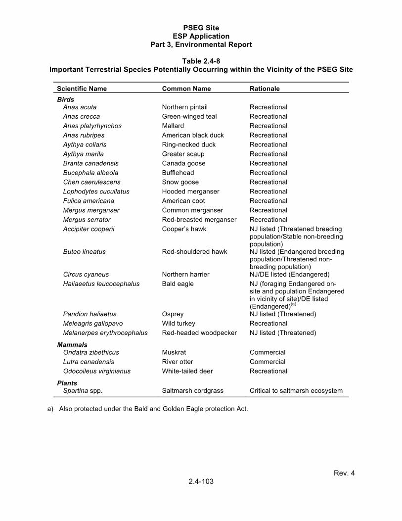
PSEG Site ESP Application
Part 3, Environmental Report
Rev. 4 2.4-103
Table 2.4-8 Important Terrestrial Species Potentially Occurring within the Vicinity of the PSEG Site
Scientific Name Common Name Rationale
Birds Anas acuta Northern pintail Recreational
Anas crecca Green-winged teal Recreational
Anas platyrhynchos Mallard Recreational
Anas rubripes American black duck Recreational
Aythya collaris Ring-necked duck Recreational
Aythya marila Greater scaup Recreational
Branta canadensis Canada goose Recreational
Bucephala albeola Bufflehead Recreational
Chen caerulescens Snow goose Recreational
Lophodytes cucullatus Hooded merganser Recreational
Fulica americana American coot Recreational
Mergus merganser Common merganser Recreational
Mergus serrator Red-breasted merganser Recreational
Accipiter cooperii Cooper’s hawk NJ listed (Threatened breeding population/Stable non-breeding population)
Buteo lineatus Red-shouldered hawk NJ listed (Endangered breeding population/Threatened non-breeding population)
Circus cyaneus Northern harrier NJ/DE listed (Endangered)
Haliaeetus leucocephalus Bald eagle NJ (foraging Endangered on-site and population Endangered in vicinity of site)/DE listed (Endangered)(a)
Pandion haliaetus Osprey NJ listed (Threatened)
Meleagris gallopavo Wild turkey Recreational
Melanerpes erythrocephalus Red-headed woodpecker NJ listed (Threatened)
Mammals Ondatra zibethicus Muskrat Commercial
Lutra canadensis River otter Commercial
Odocoileus virginianus White-tailed deer Recreational
Plants Spartina spp. Saltmarsh cordgrass Critical to saltmarsh ecosystem
a) Also protected under the Bald and Golden Eagle protection Act.

PSEG Site ESP Application
Part 3, Environmental Report
Rev. 4 2.4-104
Table 2.4-9 (Sheet 1 of 7) Terrestrial Plants Observed Seasonally On-Site and in the Vicinity of the PSEG Site, 2009
Botanical Name Common Name Taxa
Season Observed Qualitative Abundance in Area
Surveyed(a)
Ca
us
ew
ay
(b)
Ex
isti
ng
A
cc
es
s
Ro
ad
(c)
Spring Summer Fall TS
-03
TS
-04
TS
-05
TS
-06
TS
-07
TS
-08
TS
-17
TS
-18
Trees/Saplings
Acer negundo Box elder 1 1 R
Acer rubrum Red maple 1 1 1 x
Acer saccharinum Silver maple 1 1 x
Albizzia julibrissin Mimosa 1 1 1 1 x
Baccharis halimifolia Groundsel tree, sea myrtle
1 1 1 1 O C C O C x
Celtis occidentalis Hackberry 1 1 1 U
Diospyros virginiana Persimmon 1 1 1 1 x
Gleditsia triacanthos Honey locust 1 1 x
Juglans nigra Black walnut 1 1 x
Juniperus virginiana Eastern red cedar 1 1 1 1 O O O C x
Liquidambar styraciflua Sweetgum 1 1 1 x
Morus alba White mulberry 1 1 1 1 O O x
Nyssa sylvatica Blackgum 1 1 x
Paulownia tomentosa Empress tree 1 1 x
Platanus occidentalis Sycamore 1 1 x
Populus deltoides Cottonwood 1 1 1 1 R x
Populus grandidentata Bigtooth aspen 1 1 x
Prunus serotina Wild black cherry 1 1 1 1 O R O x
Quercus rubra Northern red oak 1 1 x
Robinia pseudoacacia Black locust 1 1 x
Salix nigra Black willow 1 1 1 1 x

PSEG Site ESP Application
Part 3, Environmental Report
Rev. 4 2.4-105
Table 2.4-9 (Sheet 2 of 7) Terrestrial Plants Observed Seasonally On-Site and within the Vicinity of the PSEG Site, 2009
Botanical Name Common Name Taxa
Season Observed Qualitative Abundance in Area
Surveyed(a)
Ca
us
ew
ay
(b)
Ex
isti
ng
A
cc
es
s
Ro
ad
(c)
Spring Summer Fall TS
-03
TS
-04
TS
-05
TS
-06
TS
-07
TS
-08
TS
-17
TS
-18
Trees/Saplings, cont.
Salix sp. Willow 1 x
Sassafras albidum Sassafras 1 1 1 1 x
Shrubs
Eleagnus umbellata Autumn olive 1 1 1 1 O U O C C x
Myrica cerifera Wax myrtle 1 1 x
Rhus copallinum Winged sumac 1 1 1 1 U R x
Rhus glabra Smooth sumac 1 1 1 1 R U x
Rhus typhina Staghorn sumac 1 1 1 x
Rosa multiflora Multiflora rose 1 1 1 1 O R O C O x
Rubus sp. Blackberry 1 1 U x
Sambucus canadensis Common elderberry 1 1 O
Symphoricarpos orbiculatus Coralberry 1 1 x
Viburnum dentatum Arrow-wood 1 1 1 R x
Vines
Campsis radicans Trumpet creeper 1 1 1 x
Lonicera japonica Japanese honeysuckle 1 1 1 1 C C O C x
Parthenocissus quinquefolia Virginia creeper 1 1 1 1 U O x
Toxicodendron radicans Poison ivy 1 1 1 1 C x
Vicia villosa Hairy vetch 1 1 U O
Vitis sp. Wild grape 1 1 1 x

PSEG Site ESP Application
Part 3, Environmental Report
Rev. 4 2.4-106
Table 2.4-9 (Sheet 3 of 7) Terrestrial Plants Observed Seasonally On-Site and within the Vicinity of the PSEG Site, 2009
Botanical Name Common Name Taxa
Season Observed Qualitative Abundance in Area
Surveyed(a)
Ca
us
ew
ay
(b)
Ex
isti
ng
A
cc
es
s
Ro
ad
(c)
Spring Summer Fall TS
-03
TS
-04
TS
-05
TS
-06
TS
-07
TS
-08
TS
-17
TS
-18
Herbs
Achillea millefolium Common yarrow 1 1 x
Allium canadense Onion 1 1 U
Amaranthus cannabinus Tidalmarsh amaranth 1 1 x
Ambrosia artemisiifolia Common ragweed 1 1 1 1 O C O A O
Andropogon virginicus Broomsedge 1 1 1 1 U O A A O U U x
Apocynum cannabinum Dogbane 1 1 1 1 O O O x
Arenaria serpyllifolia Thyme-leaf sandwort 1 1 U C O
Artemisia vulgaris Mugwort 1 1 1 1 A A A A C A A O x
Artemisia sp. 1 U
Asclepias syriaca Common milkweed 1 1 1 1 O U O O O x
Aster sp. 1 1 U U
Capsella bursa-pastoris Shepard's purse 1 1 O
Carex sp. Sedge 1 U
Carex stricta Upright sedge 1 1 x
Carex vulpinoidea Fox sedge 1 1 U
Cichorium intybus Chickory 1 1 1 x
Cirsium vulgare Bull thistle 1 1 1 U R x
Conyza canadensis Horseweed 1 1 1 R A U x
Cyperus strigosus False nutsedge 1 1 1 U U U
Daucus carota Queen Anne's lace 1 1 1 1 O C C C C C x
Digitaria ischaemum Smooth crabgrass 1 1 O O O U
Echinochloa crusgalli Barnyard grass 1 1 1 U U

PSEG Site ESP Application
Part 3, Environmental Report
Rev. 4 2.4-107
Table 2.4-9 (Sheet 4 of 7) Terrestrial Plants Observed Seasonally On-Site and within the Vicinity of the PSEG Site, 2009
Botanical Name Common Name Taxa
Season Observed Qualitative Abundance in Area
Surveyed(a)
Ca
us
ew
ay
(b)
Ex
isti
ng
A
cc
es
s
Ro
ad
(c)
Spring Summer Fall TS
-03
TS
-04
TS
-05
TS
-06
TS
-07
TS
-08
TS
-17
TS
-18
Herbs, cont.
Eleocharis palustris Common spike rush 1 1 1 A
Eleocharis ovata Ovate spike rush 1 1 U
Erigeron annuus Annual fleabane 1 1 1 1 C O R U
Erigeron strigosus Daisy fleabane 1 1 U
Eupatorium serotinum Late boneset 1 1 1 1 O C O U C U U x
Festuca sp. Fescue 1 1 1 1 O O A A C O x
Galium aparine Cleavers 1 1 U U x
Geranium carolinianum Carolina crane's-bill 1 1 1 O C O
Glycine max Soybean 1 1 1 x
Hordeum jubatum Foxtail barley 1 1 1 U R U R A
Humulus japonicus Japanese hops 1 1 O
Hypericum punctatum Spotted St. John's wort 1 1 U U
Impatiens capensis Orange touch-me-not 1 1 x
Juncus acuminatus Rush 1 1 O O x
Juncus effusus Soft rush 1 1 1 1 R O
Juncus tenuis Path rush 1 1 O U
Juncus torreyi Torrey's rush 1 1 O
Lactuca serriola Prickly lettuce 1 1 R
Lactuca sp. 1 U
Lamium amplexicaule Henbit 1 1 R x
Lepidium campestre Field cress 1 1 U U
Lepidium sp. Field cress 1 O
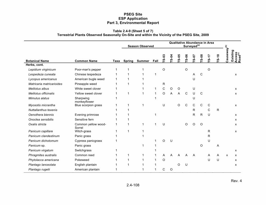
PSEG Site ESP Application
Part 3, Environmental Report
Rev. 4 2.4-108
Table 2.4-9 (Sheet 5 of 7) Terrestrial Plants Observed Seasonally On-Site and within the Vicinity of the PSEG Site, 2009
Botanical Name Common Name Taxa
Season Observed Qualitative Abundance in Area
Surveyed(a)
Ca
us
ew
ay
(b)
Ex
isti
ng
A
cc
es
s
Ro
ad
(c)
Spring Summer Fall TS
-03
TS
-04
TS
-05
TS
-06
TS
-07
TS
-08
TS
-17
TS
-18
Herbs, cont.
Lepidium virginicum Poor-man's pepper 1 1 1 O O O
Lespedeza cuneata Chinese lespedeza 1 1 1 1 A C x
Lycopus americanus American bugle weed 1 1 1 U
Matricaria matricarioides Pineapple weed 1 1 1 R
Melilotus albus White sweet clover 1 1 1 C O O U x
Melilotus officinalis Yellow sweet clover 1 1 1 1 O A A C U C x
Mimulus alatus Sharpwing monkeyflower
1 1 U
Myosotis micrantha Blue scorpion grass 1 1 1 U O C C C C x
Nuttallanthus texenis 1 1 R C R
Oenothera biennis Evening primrose 1 1 1 R R U x
Onoclea sensibilis Sensitive fern 1 1 x
Oxalis stricta Common yellow wood-Sorrel
1 1 1 1 U O O O x
Panicum capillare Witch-grass 1 1 1 R x
Panicum clandestinum Panic grass 1 1 R
Panicum dichotomum Cypress panicgrass 1 1 O U U
Panicum sp. Panic grass 1 1 O A
Panicum virgatum Switchgrass 1 1 x
Phragmites australis Common reed 1 1 1 1 A A A A A A A x x
Phytolacca americana Pokeweed 1 1 1 1 O U U x
Plantago lanceolata English plantain 1 1 1 1 O U x
Plantago rugelii American plantain 1 1 1 C O

PSEG Site ESP Application
Part 3, Environmental Report
Rev. 4 2.4-109
Table 2.4-9 (Sheet 6 of 7) Terrestrial Plants Observed Seasonally On-Site and within the Vicinity of the PSEG Site, 2009
Botanical Name Common Name Taxa
Season Observed Qualitative Abundance in Area
Surveyed(a)
Ca
us
ew
ay
(b)
Ex
isti
ng
A
cc
es
s
Ro
ad
(c)
Spring Summer Fall TS
-03
TS
-04
TS
-05
TS
-06
TS
-07
TS
-08
TS
-17
TS
-18
Herbs, cont.
Plantago virginica Plantain 1 1 1 U A C
Poa compressa Canada bluegrass 1 1 1 1 A U A x
Polygonum hydropiper Water pepper 1 1 1 U U x x
Polygonum perfoliatum Mile-a-minute vine 1 1 1 1 U U R C O x x
Polygonum persicaria Spotted ladysthumb 1 1 U
Polygonum sp. 1 U
Ranunculus scleratus Cursed crowfoot 1 1 U
Ranunculus sp. Buttercup 1 1 U x
Rumex acetosella Red sorrel 1 1 1 U C x
Rumex crispus Curly dock 1 1 1 1 C O U U x
Sagittaria latifolia Arrowhead 1 1 1 x x
Scirpus americanus Olney's-threesquare 1 1 x
Scirpus atrovirens Black bulrush 1 1 x
Scirpus robustus Sturdy bulrush 1 1 x
Scleranthus annuus Annual knawel 1 1 O
Senecio vulgaris Common groundsel 1 1 1 U x
Setaria faberi Giant foxtail grass 1 1 1 R O
Setaria viridus Green foxtail grass 1 1 C U C C
Sibara virginica Virginia rock cress 1 1 U U
Solanum carolinense Carolina horsenettle 1 1 R
Solidago altissima Canada goldenrod 1 1 1 O C C O x
Solidago graminifolia Lance-leaved goldenrod 1 1 U

PSEG Site ESP Application
Part 3, Environmental Report
Rev. 4 2.4-110
Table 2.4-9 (Sheet 7 of 7) Terrestrial Plants Observed Seasonally On-Site and within the Vicinity of the PSEG Site, 2009
Botanical Name Common Name Taxa
Season Observed Qualitative Abundance in Area
Surveyed(a)
Ca
us
ew
ay
(b)
Ex
isti
ng
A
cc
es
s
Ro
ad
(c)
Spring Summer Fall TS
-03
TS
-04
TS
-05
TS
-06
TS
-07
TS
-08
TS
-17
TS
-18
Herbs, cont.
Solidago sempervirens Seaside goldenrod 1 1 U O O x
Solidago sp. Goldenrod 1 1 O C C C O x
Spartina alterniflora Smooth cordgrass 1 1 1 x x
Spartina cynosuroides Big cordgrass 1 1 x
Spartina patens Salt-meadow cordgrass 1 1 x
Spergula morisonii Spurrey 1 1 1 O O
Taraxacum officinale Common dandelion 1 1 1 1 U x
Thlaspi arvense Field penny-cress 1 1 1 O
Tridens flavus Purpletop 1 1 1 C C x
Trifolium arvense Rabbit foot clover 1 1 U
Trifolium repens White clover 1 1 1 U x
Typha latifolia Cattail 1 1 x
Verbascum thapsus Common mullein 1 1 1 1 U U U
Viola bicolor Violet 1 1 U
Xanthium strumarium Common cocklebur 1 1 1 U U
Zea mays Corn 1 1 x
Total Taxa 134 92 91 72
a) Abundance Categories: A=abundant; C=common; O=occasional; U=uncommon; R=rare b) Surveyed by boat at selected creek locations along proposed causeway - presence/absence only, abundance categories not assigned c) Represents baseline conditions of roadside vegetation along existing access road - presence/absence only, abundance categories not assigned

PSEG Site ESP Application
Part 3, Environmental Report
Rev. 4 2.4-111
Table 2.4-10 Land Use/Land Cover (LULC) (Acres) within Each Off-Site Transmission Macro-Corridor
6-Mile
Vicinity 6 to 50+ Mile
Region Total Percent
South Corridor(a)
Open Water 4468 21,686 26,154 8%
Developed - Open Space 282 6360 6642 2%
Developed - Low Intensity 199 5696 5895 2%
Developed - Medium Intensity 90 2684 2774 1%
Developed - High Intensity 192 1394 1586 1%
Barren Land 493 3110 3603 1%
Deciduous Forest 2243 39,052 41,295 13%
Evergreen Forest 58 4106 4165 1%
Mixed Forest 11 1807 1817 1%
Pasture Hay 3416 32,175 35,591 11%
Cultivated Crops 11,704 110,191 121,895 39%
Woody Wetlands 7742 18,707 26,448 8%
Emergent Herbaceous Wetlands 11,648 26,915 38,563 12%
Total 42,545 273,884 316,429 100%
West Corridor(b)
Open Water 1976 18,744 20,721 11%
Developed - Open Space 98 7609 7706 4%
Developed - Low Intensity 97 8769 8867 5%
Developed - Medium Intensity 64 3726 3789 2%
Developed - High Intensity 191 1420 1610 1%
Barren Land 351 2570 2921 2%
Deciduous Forest 1086 33,969 35,055 18%
Evergreen Forest 13 1064 1077 1%
Mixed Forest 9 32 42 0%
Pasture Hay 934 45,122 46,055 24%
Cultivated Crops 4310 31,396 35,706 19%
Woody Wetlands 4276 11,534 15,810 8%
Emergent Herbaceous Wetlands 7675 4490 12,164 6%
Total 21,077 170,446 191,523 100%
a) Total length = 94 mi. b) Total length = 55 mi.

PSEG Site ESP Application
Part 3, Environmental Report
Rev. 4 2.4-112
Table 2.4-11
National Wetland Inventory (NWI) Wetlands within the 5-Mile Wide Macro-Corridor Study Area
South Corridor(a)
5-Mi. Wide Corridor
6-Mile Vicinity 6-50+ Mile Region TotalEstuarine and Marine Deepwater 3858 8749 12,607Estuarine and Marine Wetland 16,551 32,707 49,257Freshwater Emergent Wetland 1522 3934 5457Freshwater Forested/Shrub Wetland 1677 22,730 24,408Freshwater Pond 284 1017 1301Lake 1 766 767Riverine 17 328 344Other 63 208 271
Total 23,973 70,440 94,413West Corridor(b)
Estuarine and Marine Deepwater 2347 4333 6680Estuarine and Marine Wetland 10,121 5241 15,362Freshwater Emergent Wetland 1400 2788 4188Freshwater Forested/Shrub Wetland 1164 6173 7337Freshwater Pond 172 833 1005Lake 1 335 336Riverine 17 414 430Other 63 114 177
Total 15,285 20,231 35,516
a) Total length = 94 mi. b) Total length = 55 mi.

PSEG Site ESP Application
Part 3, Environmental Report
Rev. 4 2.4-113
Table 2.4-12 Species Composition and Abundance of Fish Collections from Ponds on the PSEG Site, by Season, 2009(b)
Scientific Name
Common Name
February(a) May July September
Stations AS
-04
AS
-09
AS
-04
AS
-09
AS
-01
4
AS
-04
AS
-09
AS
-14
AS
-04
AS
-09
AS
-01
4
Anguilla rostrata American eel 1 1 Cyprinodon variegatus Sheepshead
minnow 19 78 41 Cyprinus carpio Common carp 105 37 Fundulus diaphanus Banded killifish 50 8 6 Fundulus heteroclitus Mummichog 41 1 51 1 16 Gambusia affinis Mosquitofish 1 Lepomis gibbosus Pumpkinseed 20 34 3 230 6 27 Lepomis macrochirus Bluegill 49 50 Menidia beryllina Inland silverside 4 8 1 2 54 3 73 Micropterus salmoides Largemouth bass 1 1 10 71 Morone americana White perch 1 3
Total Number of Individuals 4 22 152 55 1 318 67 183 98 78 130
Total Number of Species 1 3 5 5 1 4 4 3 4 4 3
a) Sampling location AS-14 was established after the February 2009 sampling event and therefore no data was obtained for the winter season. Winter sampling at AS-14 could not be performed in January 2010 due to ice cover.
b) Information in this table collected as part of ESPA sampling program.

PSEG Site ESP Application
Part 3, Environmental Report
Rev. 4 2.4-114
Table 2.4-13 Taxonomic Composition and Abundance in Macroinvertebrate Surveys Collected
by Ponar Dredge in Ponds on the PSEG Site, 2009(a)
Scientific Name Spring Fall
AS-04 AS-09 AS-14 AS-04 AS-09 AS-14 PHYLUM NEMATODA
Unidentified Nematoda 1
PHYLUM ANNELIDA Class Oligochaeta Limnodrilus sp. 51 137 48 Pristina sp. 1 Unidentified Naididae 1 Unidentified Oligochaeta 1 Unidentified Tubificidae 11 185 2
PHYLUM ARTHROPODA Subphylum Crustacea
Order Amphipoda Gammarus daiberi 1 1 Order Isopoda Cyathura polita 1 Subphylum Mandibulata
Class Insecta Order Diptera
Ceratopogonidae 5 Chironomus sp. 117 6 31 Glyptotendipes sp. 1 1 Micropsectra sp. 2 Polypedilum sp. 1 Tanypus sp. 3 2 4 Tanytarsus sp. 1 Unidentified Chironomidae 2 Total Number of Individuals 195 334 84 3 1 0 Total Number of Taxa 11 8 4 2 1 0
a) Information in this table collected as part of ESPA sampling program.

PSEG Site ESP Application
Part 3, Environmental Report
Rev. 4 2.4-115
Table 2.4-14 Species Composition and Abundance of Fish Collections from Small Marsh Creeks
on or near the PSEG Site, by Season, 2009(a)
February May July September Scientific Name Common Name
AS-05 AS-06 AS-10 AS-05 AS-06 AS-10 AS-05 AS-06 AS-10 AS-05 AS-06 AS-10
Anguilla rostrata American eel 1
Brevoortia tyrannus Atlantic menhaden 31 13
Notemigonus crysoleucas Golden shiner 1
Ameiurus nebulosus Brown bullhead 2
Cyprinodon variegatus Sheepshead minnow 10
Fundulus heteroclitus Mummichog 51 56 37 49 40 16 21 16 282 11 9 56
Morone americana White perch 4 3 1
Morone saxatilis Striped bass 1 2 1 1
Gobiesoma bosc Naked goby 1
Total number of individuals 53 56 37 50 73 16 26 32 292 16 9 56
Total number of species 3 1 1 2 3 1 3 3 2 5 1 1
a) Information in this table collected as part of ESPA sampling program.

PSEG Site ESP Application
Part 3, Environmental Report
Rev. 4 2.4-116
Table 2.4-15 (Sheet 1 of 2) Taxonomic Composition and Abundance in Macroinvertebrate Surveys Collected by Ponar Dredge in Marsh Creeks
on or near the PSEG Site, 2009(a)
Scientific Name Spring 2009 Fall 2009
Large Marsh Creeks Small Marsh Creeks Large Marsh Creeks Small Marsh CreeksAS-01 AS-02 AS-03 AS-11 AS-05 AS-06 AS-10 AS-01 AS-02 AS-03 AS-11 AS-05 AS-06 AS-10
PHYLUM NEMERTEA Unidentified Nemertea 1
PHYLUM ANNELIDA Unidentified Annelida 1
Class Oligochaeta Limnodrilus sp. 15 52 19 1 Unidentified Naididae 1 Unidentified Tubificidae 29 68 11 Unidentified Oligochaeta 1 1 3
Class Polychaeta Ampharetidae 4 6 1 Marenzellaria viridis 1 1 Nereis (=Neanthes) succinea 1 21 1 Nereis virens 8 Unidentified Polychaeta 1 2 1 4 4
PHYLUM MOLLUSCA Class Pelecypoda
Mya arenaria 1 Rangea cuneata 1 Unidentified Pelecypoda 2 PHYLUM ARTHROPODA
Subphylum Crustacea Order Amphipoda
Corophium sp. 705 163 1 1 Gammarus sp. 68 1 Gammarus daiberi 33 37 11 75 Leptocheirus plumulosis 12 8 116 Photis sp. 4 Unidentified Amphipoda 4 2 3 1 2 7

PSEG Site ESP Application
Part 3, Environmental Report
Rev. 4 2.4-117
Table 2.4-15 (Sheet 2 of 2) Taxonomic Composition and Abundance in Macroinvertebrate Surveys Collected by Ponar Dredge in Marsh Creeks
on or near the PSEG Site, 2009(a)
Scientific Name Spring 2009 Fall 2009
Large Marsh Creeks Small Marsh Creeks Large Marsh Creeks Small Marsh CreeksAS-01 AS-02 AS-03 AS-11 AS-05 AS-06 AS-10 AS-01 AS-02 AS-03 AS-11 AS-05 AS-06 AS-10
Order Decapoda Callinectes sapidus 1 Hemigrapsus sanguineus 1
Order Isopoda Chiridotea almyra 3 Cyathura polita 9 1 2 Edotea triloba 1
Order Mysidacea Neomysis sp. 3 Neomysis americana 3 Subphylum Mandibulata
Class Insecta Order Diptera
Chironomus sp. 5 1 13 1 Serromyia sp. 4 Total Number of Individuals 12 756 228 26 84 401 48 3 1 1 2 1 1 1 Total Number of Taxa 4 8 8 9 11 9 5 3 1 1 2 1 1 1 a) Information in this table collected as part of ESPA sampling program.

PSEG Site ESP Application
Part 3, Environmental Report
Rev. 4 2.4-118
Table 2.4-16 (Sheet 1 of 10) Species Composition and Abundance in Fish Surveys of Small (Sampled by Weir) and Large (Sampled by Trawling) Segments of Marsh Creek Systems in the Vicinity of the
PSEG Site, 2003 – 2007
Scientific Name Common Name
2003 Mad Horse Creek Alloway Creek Mill Creek Large Small Large Small Large Small
Anguilla rostrata American eel 1 2 51 5 11 3 Alosa aestivalis Blueback herring 3 - 14 - - - Alosa mediocris Hickory shad - - - - 2 - Alosa pseudahorengus Alewife 7 - 63 - 7 2 Alosa sapidissima American shad - - 1 - - - Brevoortia tyrannus Atlantic menhaden 20 3 78 - 12 2 Clupea harengus Atlantic herring 3 - - - - - Clupea spp. Unidentified herrings - - - - - - Clupeidae Unidentified herrings - - - - - - Dorosoma cepedianum Gizzard shad - - - - 15 -
Anchoa hepsetus Broad-striped anchovy - - - - - -
Anchoa mitchilli Bay anchovy 317 10 579 8 480 1471 Carassius auratus Goldfish - - 15 - - - Cyprinus carpio Common carp - - - - 1 1
Hybognathus regius Eastern silvery minnow - - 4 1 12 1
Notemigonus crysoleucas Golden shiner - - - - - - Notropis hudsonius Spottail shiner - - 1 - - - Catostomus commersoni White sucker - - - - - - Ameiurus catus White catfish 1 - 14 - 2 - Ameiurus nebulosus Brown bullhead - - 190 - 29 9 Ictaluras punctatus Channel catfish 1 - 186 - 3 - Opsanus tau Oyster toadfish - - - - - - Fundulus heteroclitus Mummichog 76 177 1 1849 - 822 Fundulus majalis Striped killifish - - - - - 1 Lucania parva Rainwater killifish - - - - - - Menidia menidia Atlantic silverside 701 48 - 19 1 15 Syngnathus fuscus Northern pipefish 2 - 1 - - - Morone americana White perch 109 5 5329 59 686 15 Morone saxatillis Striped bass 65 3 1122 4 18 1
Morone sp. Unidentified percithyids - - 1 - 13 -
Lepomis cyanellus Green sunfish - - - - - - Lepomis gibbosus Pumpkinseed - - - - - - Lepomis macrochirus Bluegill - - 1 - - - Micropterus salmoides Largemouth bass - - - - - - Pomoxis nigromaculatus Black crappie - - - - - - Etheostoma olmstedi Tessellated darter - - - - - - Perca flavescens Yellow perch - - 3 - - - Pomatomus saltatrix Bluefish 2 - 5 - 1 - Stentotomus chrysops Scup - - 1 - - -

PSEG Site ESP Application
Part 3, Environmental Report
Rev. 4 2.4-119
Table 2.4-16 (Sheet 2 of 10) Species Composition and Abundance in Fish Surveys of Small (Sampled by Weir) and Large (Sampled by Trawling) Segments of Marsh Creek Systems in the Vicinity of the
PSEG Site, 2003 – 2007
Scientific Name Common Name
2003 Mad Horse Creek Alloway Creek Mill Creek Large Small Large Small Large Small
Bairdiella chrysoura Silver perch - - 5 1 - - Cynoscion regalis Weakfish 13 - 24 - 40 1 Leiostomus xanthurus Spot 1 - 3 - - - Menticirrhus saxatilis Northern kingfish - - - - - - Micropogonias undulatus Atlantic croaker 20 - 87 - 7 - Pogonias cromis Black drum 78 - 9 - 2 - Sciaenidae Unidentified drums - - - - - - Mugil curema White mullet - - - - - - Gobiosoma bosc Naked goby 2 92 14 5 - 5 Etropus microstomus Smallmouth flouder - - - - - - Paralichthys dentatus Summer flounder 3 1 2 - - -
Scopthalmus aquosus Windowpane flounder - - - - - -
Trinectes maculatus Hogchoker 49 - 497 - 55 -
Symphurus plagiusa Blackcheek tonguefish - - - - - -
Number of individuals 4169 502 1055 3668 1062 87 Number of species 26 11 21 17 23 7
Callinectes sapidus Blue crab 280 76 49 10 15 2

PSEG Site ESP Application
Part 3, Environmental Report
Rev. 4 2.4-120
Table 2.4-16 (Sheet 3 of 10) Species Composition and Abundance in Fish Surveys of Small (Sampled by Weir) and Large (Sampled by Trawling) Segments of Marsh Creek Systems in the Vicinity of the
PSEG Site, 2003 – 2007
Scientific Name Common Name
2004 Mad Horse
Creek Alloway Creek Mill Creek Large Small Large Small Large Small
Anguilla rostrata American eel 6 6 47 2 11 12 Alosa aestivalis Blueback herring 4 - 11 - - - Alosa mediocris Hickory shad 2 - 17 2 - - Alosa pseudahorengus Alewife 8 - 61 63 7 - Alosa sapidissima American shad - - 30 - 1 - Brevoortia tyrannus Atlantic menhaden 516 - 147 33 44 1 Clupea harengus Atlantic herring - - - - - - Clupea spp. Unidentified herrings - - - - - - Clupeidae Unidentified herrings - - - - - - Dorosoma cepedianum Gizzard shad - - - - 13 -
Anchoa hepsetus Broad-striped anchovy - - - - - -
Anchoa mitchilli Bay anchovy 553 79 370 11 722 303 Carassius auratus Goldfish - - - - - - Cyprinus carpio Common carp - - 9 - 1 5
Hybognathus regius Eastern silvery minnow - - - - 3 7
Notemigonus crysoleucas Golden shiner - - - - - 1 Notropis hudsonius Spottail shiner - - - - - - Catostomus commersoni White sucker - - - - - - Ameiurus catus White catfish - - 126 - 2 6 Ameiurus nebulosus Brown bullhead 4 - 73 5 44 31 Ictaluras punctatus Channel catfish - - 216 1 1 - Opsanus tau Oyster toadfish - - - - - - Fundulus heteroclitus Mummichog 11 197 2 708 5 4540 Fundulus majalis Striped killifish - - - - - - Lucania parva Rainwater killifish - - - - - - Menidia menidia Atlantic silverside 78 67 - 8 3 31 Syngnathus fuscus Northern pipefish 1 - 3 - - - Morone americana White perch 197 2 4176 37 811 62 Morone saxatillis Striped bass 51 - 314 2 11 -
Morone sp. Unidentified percithyids - - 10 - 2 -
Lepomis cyanellus Green sunfish - - - - - - Lepomis gibbosus Pumpkinseed - - 1 - - - Lepomis macrochirus Bluegill - - - 1 - - Micropterus salmoides Largemouth bass - - 1 - - - Pomoxis nigromaculatus Black crappie - - - - - - Etheostoma olmstedi Tessellated darter - - - - - - Perca flavescens Yellow perch - - 6 - - - Pomatomus saltatrix Bluefish 1 - 5 - 2 - Stentotomus chrysops Scup - - - - - -

PSEG Site ESP Application
Part 3, Environmental Report
Rev. 4 2.4-121
Table 2.4-16 (Sheet 4 of 10) Species Composition and Abundance in Fish Surveys of Small (Sampled by Weir) and Large (Sampled by Trawling) Segments of Marsh Creek Systems in the Vicinity of the
PSEG Site, 2003 – 2007
Scientific Name Common Name
2004 Mad Horse Creek Alloway Creek Mill Creek Large Small Large Small Large Small
Bairdiella chrysoura Silver perch 4 - 3 - - - Cynoscion regalis Weakfish 23 - 126 - 19 2 Leiostomus xanthurus Spot 1 - 6 - - - Menticirrhus saxatilis Northern kingfish - - - - - - Micropogonias undulatus Atlantic croaker 8 - 325 - 122 - Pogonias cromis Black drum 14 - 3 - 5 1 Sciaenidae Unidentified drums 1 - 2 - - - Mugil curema White mullet - - 2 - - - Gobiosoma bosc Naked goby 3 14 10 4 - - Etropus microstomus Smallmouth flouder - - - - - - Paralichthys dentatus Summer flounder 3 - 3 - - -
Scopthalmus aquosus Windowpane flounder - - - - - -
Trinectes maculatus Hogchoker 20 - 478 - 21 -
Symphurus plagiusa Blackcheek tonguefish - - - - - -
Number of individuals 1509 365 6583 877 1850 5002 Number of species 21 6 28 13 20 13
Callinectes sapidus Blue crab 231 82 71 11 30 7
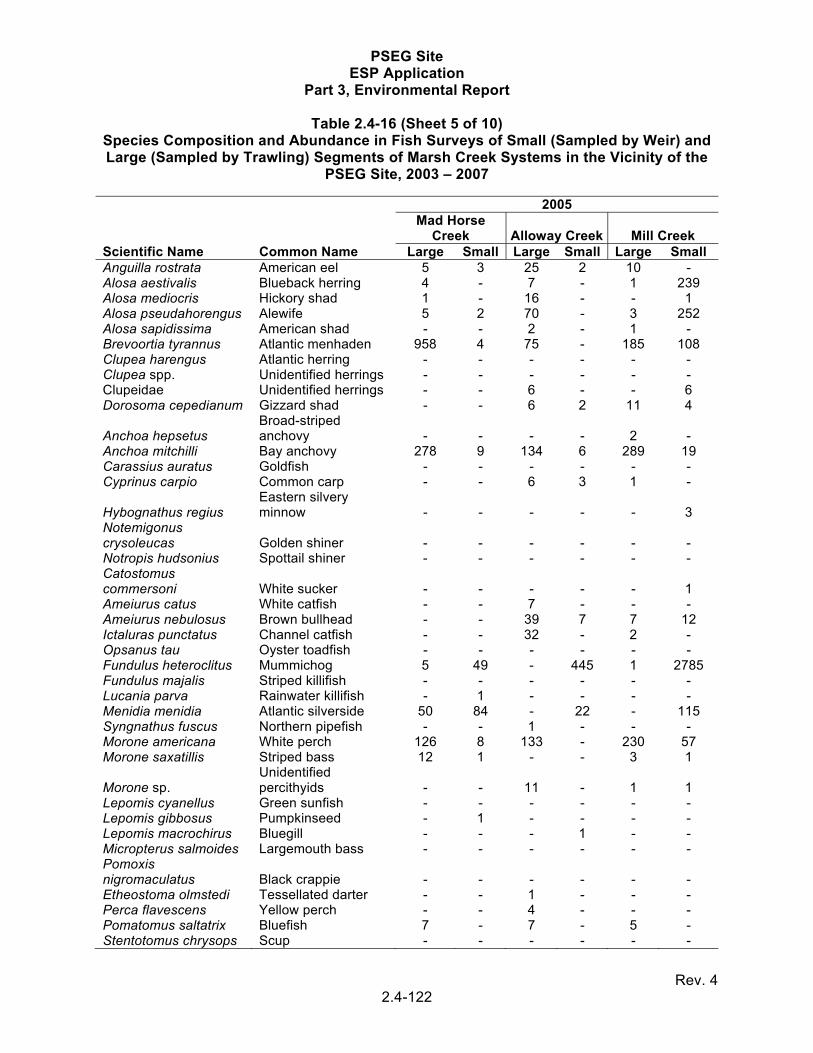
PSEG Site ESP Application
Part 3, Environmental Report
Rev. 4 2.4-122
Table 2.4-16 (Sheet 5 of 10) Species Composition and Abundance in Fish Surveys of Small (Sampled by Weir) and Large (Sampled by Trawling) Segments of Marsh Creek Systems in the Vicinity of the
PSEG Site, 2003 – 2007
Scientific Name Common Name
2005 Mad Horse
Creek Alloway Creek Mill Creek Large Small Large Small Large Small
Anguilla rostrata American eel 5 3 25 2 10 - Alosa aestivalis Blueback herring 4 - 7 - 1 239 Alosa mediocris Hickory shad 1 - 16 - - 1 Alosa pseudahorengus Alewife 5 2 70 - 3 252 Alosa sapidissima American shad - - 2 - 1 - Brevoortia tyrannus Atlantic menhaden 958 4 75 - 185 108 Clupea harengus Atlantic herring - - - - - - Clupea spp. Unidentified herrings - - - - - - Clupeidae Unidentified herrings - - 6 - - 6 Dorosoma cepedianum Gizzard shad - - 6 2 11 4
Anchoa hepsetus Broad-striped anchovy - - - - 2 -
Anchoa mitchilli Bay anchovy 278 9 134 6 289 19 Carassius auratus Goldfish - - - - - - Cyprinus carpio Common carp - - 6 3 1 -
Hybognathus regius Eastern silvery minnow - - - - - 3
Notemigonus crysoleucas Golden shiner - - - - - - Notropis hudsonius Spottail shiner - - - - - - Catostomus commersoni White sucker - - - - - 1 Ameiurus catus White catfish - - 7 - - - Ameiurus nebulosus Brown bullhead - - 39 7 7 12 Ictaluras punctatus Channel catfish - - 32 - 2 - Opsanus tau Oyster toadfish - - - - - - Fundulus heteroclitus Mummichog 5 49 - 445 1 2785 Fundulus majalis Striped killifish - - - - - - Lucania parva Rainwater killifish - 1 - - - - Menidia menidia Atlantic silverside 50 84 - 22 - 115 Syngnathus fuscus Northern pipefish - - 1 - - - Morone americana White perch 126 8 133 - 230 57 Morone saxatillis Striped bass 12 1 - - 3 1
Morone sp. Unidentified percithyids - - 11 - 1 1
Lepomis cyanellus Green sunfish - - - - - - Lepomis gibbosus Pumpkinseed - 1 - - - - Lepomis macrochirus Bluegill - - - 1 - - Micropterus salmoides Largemouth bass - - - - - - Pomoxis nigromaculatus Black crappie - - - - - - Etheostoma olmstedi Tessellated darter - - 1 - - - Perca flavescens Yellow perch - - 4 - - - Pomatomus saltatrix Bluefish 7 - 7 - 5 - Stentotomus chrysops Scup - - - - - -

PSEG Site ESP Application
Part 3, Environmental Report
Rev. 4 2.4-123
Table 2.4-16 (Sheet 6 of 10) Species Composition and Abundance in Fish Surveys of Small (Sampled by Weir) and Large (Sampled by Trawling) Segments of Marsh Creek Systems in the Vicinity of the
PSEG Site, 2003 – 2007
Scientific Name Common Name
2005 Mad Horse
Creek Alloway Creek Mill Creek Large Small Large Small Large Small
Bairdiella chrysoura Silver perch 18 - 20 - 1 - Cynoscion regalis Weakfish 14 - 358 - 6 11 Leiostomus xanthurus Spot 86 13 622 5 252 47 Menticirrhus saxatilis Northern kingfish - - - - - - Micropogonias undulatus Atlantic croaker 26 - 330 7 28 - Pogonias cromis Black drum 30 - 44 - 13 3 Sciaenidae Unidentified drums 1 - - - - - Mugil curema White mullet - - - - - - Gobiosoma bosc Naked goby - 1 5 2 - 3 Etropus microstomus Smallmouth flouder - - - - - - Paralichthys dentatus Summer flounder - - 1 - - -
Scopthalmus aquosus Windowpane flounder - - - - - -
Trinectes maculatus Hogchoker 8 - 127 - 3 -
Symphurus plagiusa Blackcheek tonguefish - - - - - -
Number of individuals 1634 176 4169 502 1055 3668 Number of species 17 12 26 11 21 17
Callinectes sapidus Blue crab 375 176 115 45 29 46

PSEG Site ESP Application
Part 3, Environmental Report
Rev. 4 2.4-124
Table 2.4-16 (Sheet 7 of 10) Species Composition and Abundance in Fish Surveys of Small (Sampled by Weir) and Large (Sampled by Trawling) Segments of Marsh Creek Systems in the Vicinity of the
PSEG Site, 2003 – 2007
Scientific Name Common Name
2006 Mad Horse
Creek Alloway Creek Mill Creek Large Small Large Small Large Small
Anguilla rostrata American eel 6 1 NS 1 9 1 Alosa aestivalis Blueback herring - - NS - - - Alosa mediocris Hickory shad - - NS - - - Alosa pseudahorengus Alewife - - NS - - - Alosa sapidissima American shad 2 - NS - - - Brevoortia tyrannus Atlantic menhaden 9 11 NS 2 52 32 Clupea harengus Atlantic herring - - NS - - - Clupea spp. Unidentified herrings - - NS - - - Clupeidae Unidentified herrings - - NS - - - Dorosoma cepedianum Gizzard shad 3 - NS 1 36 31
Anchoa hepsetus Broad-striped anchovy - - NS - - -
Anchoa mitchilli Bay anchovy 254 12 NS 1 702 77 Carassius auratus Goldfish - - NS - - - Cyprinus carpio Common carp - - NS - 7 1
Hybognathus regius Eastern silvery minnow - - NS - 1 -
Notemigonus crysoleucas Golden shiner - - NS - - - Notropis hudsonius Spottail shiner - - NS - - - Catostomus commersoni White sucker - - NS - - - Ameiurus catus White catfish 1 - NS - - - Ameiurus nebulosus Brown bullhead 1 - NS 4 119 74 Ictaluras punctatus Channel catfish 3 - NS - 4 1 Opsanus tau Oyster toadfish 1 - NS - - - Fundulus heteroclitus Mummichog 19 50 NS 1178 3 1565 Fundulus majalis Striped killifish - - NS - - - Lucania parva Rainwater killifish - - NS - - - Menidia menidia Atlantic silverside 3 2 NS 7 - 58 Syngnathus fuscus Northern pipefish - - NS - - - Morone americana White perch 485 9 NS 10 1305 67 Morone saxatillis Striped bass 16 - NS - 9 1
Morone sp. Unidentified percithyids - - NS - - -
Lepomis cyanellus Green sunfish - - NS - 1 - Lepomis gibbosus Pumpkinseed - - NS - - - Lepomis macrochirus Bluegill - - NS - - - Micropterus salmoides Largemouth bass - - NS - - - Pomoxis nigromaculatus Black crappie - - NS - 1 - Etheostoma olmstedi Tessellated darter - - NS - - - Perca flavescens Yellow perch - - NS - - - Pomatomus saltatrix Bluefish - - NS - 3 1 Stentotomus chrysops Scup - - NS - - -

PSEG Site ESP Application
Part 3, Environmental Report
Rev. 4 2.4-125
Table 2.4-16 (Sheet 8 of 10) Species Composition and Abundance in Fish Surveys of Small (Sampled by Weir) and Large (Sampled by Trawling) Segments of Marsh Creek Systems in the Vicinity of the
PSEG Site, 2003 – 2007
Scientific Name Common Name
2006 Mad Horse
Creek Alloway Creek Mill Creek Large Small Large Small Large Small
Bairdiella chrysoura Silver perch 10 - NS - 1 - Cynoscion regalis Weakfish 9 - NS - 6 - Leiostomus xanthurus Spot 4 - NS - 88 - Menticirrhus saxatilis Northern kingfish 1 - NS - - - Micropogonias undulatus Atlantic croaker 190 - NS 2 656 5 Pogonias cromis Black drum - - NS - - - Sciaenidae Unidentified drums - - NS - - - Mugil curema White mullet - - NS - - - Gobiosoma bosc Naked goby 2 2 NS 1 - 1 Etropus microstomus Smallmouth flouder - - NS - - - Paralichthys dentatus Summer flounder 1 - NS - - -
Scopthalmus aquosus Windowpane flounder 1 - NS - - -
Trinectes maculatus Hogchoker 40 - NS - 3 -
Symphurus plagiusa Blackcheek tonguefish 1 - NS - - -
Number of individuals 1062 87 NS 1207 3006 1915 Number of species 23 7 NS 10 19 14
Callinectes sapidus Blue crab 572 275 NS 122 90 137

PSEG Site ESP Application
Part 3, Environmental Report
Rev. 4 2.4-126
Table 2.4-16 (Sheet 9 of 10) Species Composition and Abundance in Fish Surveys of Small (Sampled by Weir) and Large (Sampled by Trawling) Segments of Marsh Creek Systems in the Vicinity of the
PSEG Site, 2003 – 2007
Scientific Name Common Name
2007 Mad Horse
Creek Alloway Creek Mill Creek Large Small Large Small Large Small
Anguilla rostrata American eel 16 7 NS 1 10 3 Alosa aestivalis Blueback herring - - NS - 11 - Alosa mediocris Hickory shad - - NS - 1 - Alosa pseudahorengus Alewife 1 - NS - 9 - Alosa sapidissima American shad 10 - NS - 15 - Brevoortia tyrannus Atlantic menhaden 65 15 NS - 84 72 Clupea harengus Atlantic herring - - NS - - - Clupea spp. Unidentified herrings - - NS - 1 - Clupeidae Unidentified herrings - - NS - - - Dorosoma cepedianum Gizzard shad - - NS - 141 46
Anchoa hepsetus Broad-striped anchovy - - NS - - -
Anchoa mitchilli Bay anchovy 305 10 NS - 568 82 Carassius auratus Goldfish - - NS - - 1 Cyprinus carpio Common carp - - NS - 5 4
Hybognathus regius Eastern silvery minnow - - NS - 1 3
Notemigonus crysoleucas Golden shiner - - NS - - - Notropis hudsonius Spottail shiner - - NS - - - Catostomus commersoni White sucker - - NS - - - Ameiurus catus White catfish 4 - NS - - - Ameiurus nebulosus Brown bullhead 2 - NS 3 49 23 Ictaluras punctatus Channel catfish 4 - NS - 2 - Opsanus tau Oyster toadfish - - NS - - - Fundulus heteroclitus Mummichog - 20 NS 582 - 2693 Fundulus majalis Striped killifish - - NS - - - Lucania parva Rainwater killifish - - NS - - - Menidia menidia Atlantic silverside 75 15 NS 8 4 106 Syngnathus fuscus Northern pipefish - - NS - 1 - Morone americana White perch 210 3 NS 5 1040 19 Morone saxatillis Striped bass 60 - NS - 40 -
Morone sp. Unidentified
percithyids 33 - NS - 4 - Lepomis cyanellus Green sunfish - - NS - - - Lepomis gibbosus Pumpkinseed - - NS - - - Lepomis macrochirus Bluegill - - NS - - - Micropterus salmoides Largemouth bass - - NS - - - Pomoxis nigromaculatus Black crappie - - NS - - - Etheostoma olmstedi Tessellated darter - - NS - - - Perca flavescens Yellow perch - NS - - - Pomatomus saltatrix Bluefish - - NS - 2 1 Stentotomus chrysops Scup - - NS - - -

PSEG Site ESP Application
Part 3, Environmental Report
Rev. 4 2.4-127
Table 2.4-16 (Sheet 10 of 10) Species Composition and Abundance in Fish Surveys of Small (Sampled by Weir) and Large (Sampled by Trawling) Segments of Marsh Creek Systems in the Vicinity of the
PSEG Site, 2003 – 2007
Scientific Name Common Name
2007 Mad Horse
Creek Alloway Creek Mill Creek Large Small Large Small Large Small
Bairdiella chrysoura Silver perch 2 - NS - - - Cynoscion regalis Weakfish 22 - NS - 31 - Leiostomus xanthurus Spot 30 - NS - 53 6 Menticirrhus saxatilis Northern kingfish - - NS - - - Micropogonias undulatus Atlantic croaker 50 - NS - 113 - Pogonias cromis Black drum 82 - NS - 46 2 Sciaenidae Unidentified drums 1 - NS - - - Mugil curema White mullet - - NS - - - Gobiosoma bosc Naked goby 10 2 NS 5 1 5 Etropus microstomus Smallmouth flouder 6 - NS - - - Paralichthys dentatus Summer flounder 2 - NS - - -
Scopthalmus aquosus Windowpane flounder - - NS - - -
Trinectes maculatus Hogchoker 59 - NS - 11 -
Symphurus plagiusa Blackcheek tonguefish - - NS - - -
Number of individuals 1049 72 NS 604 2243 3066 Number of species 20 7 NS 6 23 15
Callinectes sapidus Blue crab 578 193 NS 65 129 112
References 2.4-159 through 2.4-163
NS – Not Sampled

PSEG Site ESP Application
Part 3, Environmental Report
Rev. 4 2.4-128
Table 2.4-17 (Sheet 1 of 3) Species Composition and Density (#/106 m3) in Impingement Samples at SGS,
2003 – 2007
Scientific Name Common Name Study Year 5-Year
Mean2003 2004 2005 2006 2007 Petromyzon marinus
Sea lamprey 0.74 0.14 0.28 0.21 0.57 0.4
Acipenser oxyrhynchus
Atlantic sturgeon 0.05 0.05 0.1
Anguila rostrata American eel 2.79 4.12 4.2 4.39 5.75 4.3Conger oceanicus Conger eel 0.07 0.28 0.05 0.1Alosa aestivalis Blueback herring 23.27 156.55 19.75 25.37 17.76 48.5Alosa pseudoharengus
Alewife 4.84 25.99 8.19 2.41 7.66 9.8
Alosa sapidissima American shad 6.43 43.24 10.11 4.01 16.98 16.2Brevoortia tyrannus
Atlantic menhaden 6.26 4.82 22.22 44.00 27.49 21.0
Clupea harengus Atlantic herring 0.21 0.2Dorosoma cepedianum
Gizzard shad 21.05 26.61 53.11 22.43 87.22 42.1
Anchoa hepsetus Striped anchovy 0.11 0.07 0.11 0.36 0.2Anchoa mitchilli Bay anchovy 89.5 93.89 49.33 202.44 132.62 113.6Umbra pygmnea Eastern
mudminnow 0.07 0.05 0.05 0.1
Cyprinus carpio Common carp 0.17 0.17 0.07 0.05 0.1Hybognathus regis Silvery minnow 16.67 16.67 5.37 4.66 2.85 9.2Notemingonus crysoleucas
Golden shiner 0.21 0.05 0.1
Ameiurus catus White catfish 0.06 0.21 0.1 0.1Ameiurus nebulosis
Brown bullhead 1.71 2.31 0.28 0.11 0.31 0.9
Ictalurus punctatus
Channel catfish 4.84 14.74 2.55 1.28 32.77 11.2
Synodus foetens Inshore lizardfish 0.07 0.1 0.1Opsanus tau Oyster toadfish 0.28 0.28 1.31 2.89 2.33 1.4Lophius americanus
Goosefish 0.06 0.1
Urophycis chuss Red hake 10.81 10.8Urophycis regia Spotted hake 59.17 159.97 24.15 267.32 11.75 104.5Merluccius bilinearis
Silver hake 0.11 0.07 0.16 0.1
Ophidion marginatum
Striped cusk-eel 12.8 5.45 31.92 3.16 12.63 13.2
Strongylura marina
Atlantic needlefish 0.51 0.28 0.21 0.11 0.1 0.2
Cyprinodon variegatus
Sheepshead minnow
0.14 0.07 0.1
Fundulus heteroclitus
Mummichog 1.59 1.82 0.62 0.48 1.81 1.3
Fundulus majalis Striped killifish 1.19 1.26 0.83 3.32 0.16 1.4Membras martinica
Rough silverside 0.7 0.34 0.21 0.4
Menidia beryllina Inland silverside 0.14 0.48 0.3Menidia menidia Atlantic silverside 35.67 25.71 24.08 46.89 44.52 35.4

PSEG Site ESP Application
Part 3, Environmental Report
Rev. 4 2.4-129
Table 2.4-17 (Sheet 2 of 3) Species Composition and Density (#/106 m3) in Impingement Samples at SGS,
2003 – 2007
Scientific Name Common Name Study Year 5-Year
Mean2003 2004 2005 2006 2007Gasterosteus aculeatus
Threespine stickleback
0.17 4.89 0.55 0.11 0.05 1.2
Hippocampus erectus
Lined seahorse 0.07 0.14 0.05 0.1
Syngnathus fuscus
Northern pipefish 3.47 2.03 1.93 2.46 4.5 2.9
Prionotus carolinus
Northern sea robin 0.63 0.77 2.68 23.82 5.9 6.8
Prionotus evolans Striped sea robin 0.46 0.21 0.07 0.2Morone americana
White perch 1771.18 2113.19 1042.62 360.51 429.81 1143.5
Morone saxatilus Striped bass 159.93 110.86 29.72 10.22 47.88 71.7Centropristis striata
Black sea bass 0.06 0.54 0.31 0.3
Lepomis cyanellus Green sunfish 0.07 0.1Lepomis gibbosus Pumpkinseed 0.06 0.07 0.16 0.1 0.1Lepomis macrochirus
Bluegill 1.59 3.28 2.48 3.91 1.5 2.6
Lepomis microlophus
Redeared sunfish 0.06 0.07 0.1
Micropterus salmoides
Largemouth bass 0.05 0.1
Pomoxis annularis White crappie 0.05 0.1Pomoxis nigromaculatus
Black crappie 0.06 0.14 0.1
Perca flavescens Yellow perch 1.59 2.58 1.93 1.12 6.21 2.7Pomatomus saltatrix
Bluefish 8.14 11.67 2.06 7.44 2.95 6.5
Caranx hippos Crevalle jack 0.06 0.14 0.14 0.11 0.1Selene vomer Lookdown 0.06 0.16 0.05 0.1Trachinotus carolinus
Florida pompano 0.05 0.1
Trachinotus falcatus
Permit 0.06 0.1
Archosargus probatocephalus
Sheepshead 0.11 0.05 0.1
Stenotomus chrysops
Scup 3.91 0.1 2.0
Bairdiella chrysoura
Silver perch 0.11 9.15 7.22 12.26 4.71 6.7
Cynoscion regalis Weakfish 530.71 725.72 930.88 343.81 379.65 582.2Leiostomus xanthurus
Spot 0.8 0.14 55.11 10.38 3.73 14.0
Menticirrhus saxatilis
Northern kingfish 16.28 7.36 3.69 18.95 11.6
Micropogonias undulatus
Atlantic croaker 101.22 626.74 845.57 1405.31 951.09 786.0
Pogonias cromis Black drum 0.85 0.07 8.26 0.21 5.85 3.0

PSEG Site ESP Application
Part 3, Environmental Report
Rev. 4 2.4-130
Table 2.4-17 (Sheet 3 of 3) Species Composition and Density (#/106 m3) in Impingement Samples at SGS,
2003 – 2007
Scientific Name Common Name
Study Year 5-Year Mean2003 2004 2005 2006 2007
Chaetodipterus faber
Atlantic spadefish 0.1 0.1
Chaetodon ocellatus
Spotfin butterflyfish 0.06 1.45 0.21 0.6
Mugil cephalus Striped mullet 0.68 0.7
Mugil curema White mullet 0.55 0.6
Tautoga onilis Tautog 0.07 0.05 0.1
Astroscopus guttatus
Northern stargazer 0.06 0.07 0.05 0.41 0.1
Hypsoblennius hentz
Feather blenny 0.05 0.1
Gobiosoma bosci Naked goby 4.1 5.87 2.61 1.5 2.43 3.3
Dormitator maculatus
Fat sleeper 0.05 0.1
Peprilus alepidotus Harvestfish 0.78 0.8
Peprilus triacanthus Butterfish 0.46 1.82 1.1
Scomberomorus maculatus
Spanish mackerel 0.07 0.1
Etropus microstomus
Smallmouth flounder 0.23 0.14 0.14 0.75 19.52 4.2
Paralichthys dentatus
Summer flounder 2.5 4.82 0.83 7.82 3.42 3.9
Paralichthys oblongus
Fourspot flounder 0.14 0.1
Scophthalmus aquosus
Windowpane flounder 3.19 2.51 0.96 10.71 0.1 3.5
Pseudopleuronectes americanus
Winter flounder 1.31 0.14 1.17 1.77 1.1
Trinectes maculatus Hogchoker 102.3 99.4 136.57 184.72 126.98 130.0
Symphurus plagiusa Blackcheek tonguefish 0.06 0.05 0.31 0.1
Sphoeroides maculatus
Northern puffer 0.06 0.05 0.05 0.1
Total density 2986.1 4330.6 3341.6 3044.4 2424.1 3243.3
Number of species 56 57 50 61 58 56.4
Callinectes sapidus Blue crab 76.4 171.3 1895.8 694.7 797.7 727.2
References 2.4-159 through 2.4-163

PSEG Site
ESP Application Part 3, Environmental Report
Rev. 4 2.4-131
Table 2.4-18 (Sheet 1 of 5) Comparison of Species Composition and Mean Density (#/106 m3) in Impingement and Entrainment Samples at SGS,
5-Year Mean (2003 – 2007) Versus 13-Year Mean (1995 – 2007)
Scientific Name Common Name
Impingement Entrainment
5-Year Mean
13-Year Mean
Occurrence Frequency*
5-Year Mean
13-Year Mean
Occurrence Frequency(a)
Petromyzon marinus Sea lamprey 0.4 0.5 Mustelus canis Smooth dogfish 0.0 0.0 1 Rhinoptera bonasus Cownose ray 0.0 0.0 1 Acipenser oxyrhynchus Atlantic sturgeon 0.1 0.0 Anguila rostrata American eel 4.3 5.4 8 0.1 0.1 8 Conger oceanicus Conger eel 0.1 0.3 5 0.0 1 Alosa aestivalis Blueback herring 48.5 62.5 8 0.0 0.0 6 Alosa pseudoharengus Alewife 9.8 12.2 8 0.0 0.0 3 Alosa sapidissima American shad 16.2 8.5 8 0.0 3 Brevoortia tyrannus Atlantic menhaden 21.0 30.6 8 1.6 1.8 8 Clupea harengus Atlantic herring 0.2 3.7 7 0.0 0.0 5 Dorosoma cepedianum Gizzard shad 42.1 39.3 8 0.0 5 Opisthonema oglinum Atlantic thread herring 0.0 0.0 1 Anchoa hepsetus Striped anchovy 0.2 0.2 5 0.0 1 Anchoa mitchilli Bay anchovy 113.6 136.6 8 88.7 74.6 8 Umbra pygmnea Eastern mudminnow 0.1 0.0 Cyprinus carpio Common carp 0.1 0.1 3 0.0 0.0 3 Hybognathus regius Silvery minnow 9.2 4.3 7 0.0 0.0 1 Notemingonus crysoleucas Golden shiner 0.1 0.0 2 Notropis analostanus Satinfin shiner 0.0 0.0 1 Notropis hudsonius Spottail shiner 0.0 0.0 1 Carpiodes cyprinus Quillback carpsucker 0.0 0.1 0.0 Catostomus commersoni White sucker 0.0 0.0 2 0.0 0.0

PSEG Site
ESP Application Part 3, Environmental Report
Rev. 4 2.4-132
Table 2.4-18 (Sheet 2 of 5) Comparison of Species Composition and Mean Density (#/106 m3) in Impingement and Entrainment Samples at SGS,
5-Year Mean (2003 – 2007) Versus 13-Year Mean (1995 – 2007)
Scientific Name Common Name
Impingement Entrainment
5-Year Mean
13-Year Mean
Occurrence Frequency*
5-Year Mean
13-Year Mean
Occurrence Frequency(a)
Ameiurus catus White catfish 0.1 0.1 4 Ameiurus nebulosis Brown bullhead 0.9 0.8 8 Ictalurus punctatus Channel catfish 11.2 4.8 8 0.0 0.0 Oncorhynchus mykiss Rainbow trout 0.0 0.0 1 Osmerus mordax Rainbow smelt 0.0 0.0 1 Synodus foetens Inshore lizardfish 0.1 0.0 2 0.0 0.0 2 Opsanus tau Oyster toadfish 1.4 3.7 8 0.0 0.0 2 Lophius americanus Goosefish 0.1 0.0 2 Gobiesox strumosus Skilletfish 0.0 0.0 2 Urophycis chuss Red hake 10.8 1.0 2 Urophycis regia Spotted hake 104.5 144.3 8 0.0 0.0 4 Merluccius bilinearis Silver hake 0.1 0.2 6 Ophidion marginatum Striped cusk-eel 13.2 19.6 8 0.0 0.0 3 Strongylura marina Atlantic needlefish 0.2 0.2 5 0.0 0.0 5 Cyprinodon variegatus Sheepshead minnow 0.1 0.0 2 0.0 0.0 Fundulus diaphanus Banded killifish 0.0 0.1 3 0.0 0.0 Fundulus heteroclitus Mummichog 1.3 2.2 8 0.0 0.0 6 Fundulus luceia Spotfin killifish 0.0 0.0 2 Fundulus majalis Striped killifish 1.4 1.1 0.0 0.0 Membras martinica Rough silverside 0.4 0.1 1 0.1 0.0 2 Menidia beryllina Inland silverside 0.3 0.1 1 0.2 0.1 1 Menidia menidia Atlantic silverside 35.4 46.0 8 0.3 0.5 8 Apeltes quadraticus Fourspine stickleback 0.0 0.1 3

PSEG Site
ESP Application Part 3, Environmental Report
Rev. 4 2.4-133
Table 2.4-18 (Sheet 3 of 5) Comparison of Species Composition and Mean Density (#/106 m3) in Impingement and Entrainment Samples at SGS,
5-Year Mean (2003 – 2007) Versus 13-Year Mean (1995 – 2007)
Scientific Name Common Name
Impingement Entrainment
5-Year Mean
13-Year Mean
Occurrence Frequency*
5-Year Mean
13-Year Mean
Occurrence Frequency(a)
Gasterosteus aculeatus Threespine stickleback 1.2 29.8 8 0.0 1 Fistularia tabacaria Bluespotted cornetfish 0.0 0.0 2 Hippocampus erectus Lined seahorse 0.1 0.1 6 Syngnathus fuscus Northern pipefish 2.9 3.6 8 0.1 0.2 8 Prionotus carolinus Northern sea robin 6.8 11.1 8 0.0 0.0 3 Prionotus evolans Striped sea robin 0.2 0.7 2 0.0 0.0 2 Morone americana White perch 1143.5 792.4 8 0.6 1.2 7 Morone saxatilus Striped bass 71.7 63.6 8 10.8 7.4 8 Centropristis striata Black sea bass 0.3 0.6 6 Acantharchus pomotis Mud sunfish 0.0 1 Lepomis auritus Redbreast sunfish 0.0 0.0 1 Lepomis cyanellus Green sunfish 0.1 0.0 Lepomis gibbosus Pumpkinseed 0.1 0.1 6 Lepomis macrochirus Bluegill 2.6 1.8 7 0.0 0.0 1 Lepomis microlophus Redeared sunfish 0.1 0.0 Micropterus salmoides Largemouth bass 0.1 0.0 Pomoxis annularis White crappie 0.1 0.0 1 0.0 1 Pomoxis nigromaculatus Black crappie 0.1 0.1 4 Orthopristis chrysoptera Pigfish 0.0 0.0 1 Etheostoma olmstedi Tessellated darter 0.0 0.0 2 Perca flavescens Yellow perch 2.7 8.2 8 0.0 0.0 4 Pomatomus saltatrix Bluefish 6.5 5.6 8 0.0 2 Caranx hippos Crevalle jack 0.1 0.2 5

PSEG Site
ESP Application Part 3, Environmental Report
Rev. 4 2.4-134
Table 2.4-18 (Sheet 4 of 5) Comparison of Species Composition and Mean Density (#/106 m3) in Impingement and Entrainment Samples at SGS,
5-Year Mean (2003 – 2007) Versus 13-Year Mean (1995 – 2007)
Scientific Name Common Name
Impingement Entrainment
5-Year Mean
13-Year Mean
Occurrence Frequency*
5-Year Mean
13-Year Mean
Occurrence Frequency(a)
Selene vomer Lookdown 0.1 0.1 2 Trachinotus carolinus Florida pompano 0.1 0.0 3 Trachinotus falcatus Permit 0.1 0.0 2 Eucinostomus argenteus Spotfin mojarra 0.0 0.0 2 Archosargus probatocephalus Sheepshead 0.1 0.0 2 Lagodon rhomboides Pinfish 0.0 0.0 1 Stenotomus chrysops Scup 2.0 0.3 1 Bairdiella chrysoura Silver perch 6.7 4.5 8 0.0 0.0 2 Cynoscion regalis Weakfish 582.2 586.1 8 1.2 2.8 8 Leiostomus xanthurus Spot 14.0 14.2 8 0.1 0.0 6 Menticirrhus americanus Southern kingfish 0.0 0.0 1 Menticirrhus saxatilis Northern kingfish 11.6 4.2 8 0.0 0.0 Micropogonias undulatus Atlantic croaker 786.0 946.6 8 5.9 7.0 8 Pogonias cromis Black drum 3.0 4.8 6 0.0 0.0 2 Chaetodipterus faber Atlantic spadefish 0.1 0.0 2 Chaetodon ocellatus Spotfin butterflyfish 0.6 0.2 4 Mugil cephalus Striped mullet 0.7 0.1 3 Mugil curema White mullet 0.6 0.0 1 Tautoga onilis Tautog 0.1 0.0 0.0 0.0 Ammodytes americanus American sand lance 0.0 0.0 0.0 1 Astroscopus guttatus Northern stargazer 0.1 0.3 5 0.0 1 Trichiurus lepturus Atlantic cutlassfish 0.0 0.0 1 Hypsoblennius hentz Feather blenny 0.1 0.0 2 0.0 3

PSEG Site
ESP Application Part 3, Environmental Report
Rev. 4 2.4-135
Table 2.4-18 (Sheet 5 of 5) Comparison of Species Composition and Mean Density (#/106 m3) in Impingement and Entrainment Samples at SGS,
5-Year Mean (2003 – 2007) Versus 13-Year Mean (1995 – 2007)
Scientific Name Common Name
Impingement Entrainment
5-Year Mean
13-Year Mean
Occurrence Frequency*
5-Year Mean
13-Year Mean
Occurrence Frequency(a)
Gobiosoma bosc Naked goby 3.3 3.3 8 32.7 28.5 8
Microgobius thalassinus Green goby 0.0 0.0 1 0.0 0.0
Dormitator maculatus Fat sleeper 0.1 0.0
Peprilus alepidotus Harvestfish 0.8 0.3 3
Peprilus triacanthus Butterfish 1.1 0.7 8 Scomberomorus maculates Spanish mackerel 0.1 0.0 3 0.0 1
Etropus microstomus Smallmouth flounder 4.2 2.0 7 0.0 0.0 4
Paralichthys dentatus Summer flounder 3.9 4.7 8 0.1 0.1 7
Paralichthys oblongus Fourspot flounder 0.1 0.0 1
Scophthalmus aquosus Windowpane flounder 3.5 2.4 7 0.0 0.0 2 Pseudopleuronectes americanus Winter flounder 1.1 2.4 8 0.0 0.0 4
Trinectes maculatus Hogchoker 130.0 223.3 8 0.1 0.1 8
Symphurus plagiusa Blackcheek tonguefish 0.1 0.1 2 0.0 0.0 3
Sphoeroides maculatus Northern puffer 0.1 0.1 3 0.0 0.0 2
Total density 3243 3247.2 142.7 124.4
Number of species 82 104 47 57
a) Number of years in the period 1995 - 2002 in which the species was encountered.
References 2.4-153 through 2.4-157 and 2.4-159 through 2.4-166.

PSEG Site ESP Application
Part 3, Environmental Report
Rev. 4 2.4-136
Table 2.4-19 (Sheet 1 of 3)
Comparison of Species Composition and Density (#/106 m3) Between Impingement Samples at SGS (2003 – 2007) and Samples at HCGS (1986 – 1987)
Scientific Name Common Name SGS 5-Year
Mean HCGS
1986-1987
Petromyzon marinus Sea lamprey 0.4 0.1
Acipenser oxyrhynchus Atlantic sturgeon 0.1
Anguila rostrata American eel 4.3 19.7
Conger oceanicus Conger eel 0.1 0.6
Alosa aestivalis Blueback herring 48.5 5.3
Alosa pseudoharengus Alewife 9.8 1.1
Alosa sapidissima American shad 16.2 0.2
Brevoortia tyrannus Atlantic menhaden 21.0 4.9
Clupea harengus Atlantic herring 0.2
Dorosoma cepedianum Gizzard shad 42.1 2.0
Anchoa hepsetus Striped anchovy 0.2 0.2
Anchoa mitchilli Bay anchovy 113.6 521.5
Umbra pygmnea Eastern mudminnow 0.1 1.5
Cyprinus carpio Common carp 0.1
Hybognathus regius Silvery minnow 9.2
Notemingonus crysoleucas Golden shiner 0.1
Ameiurus catus White catfish 0.1 0.1
Ameiurus nebulosis Brown bullhead 0.9 2.2
Ictalurus punctatus Channel catfish 11.2 1.0
Synodus foetens Inshore lizardfish 0.1
Opsanus tau Oyster toadfish 1.4 46.5
Lophius americanus Goosefish 0.1
Urophycis chuss Red hake 10.8 0.9
Urophycis regia Spotted hake 104.5 12.5
Merluccius bilinearis Silver hake 0.1 0.1
Ophidion marginatum Striped cusk-eel 13.2 27.2
Strongylura marina Atlantic needlefish 0.2
Cyprinodon variegatus Sheepshead minnow 0.1 0.6
Fundulus diaphanus Banded killifish 0.0 2.2
Fundulus heteroclitus Mummichog 1.3 1.9
Fundulus majalis Striped killifish 1.4 0.5
Membras martinica Rough silverside 0.4
Menidia beryllina Inland silverside 0.3 3.5
Menidia menidia Atlantic silverside 35.4 17.3
Gasterosteus aculeatus Threespine stickleback 1.2 1.8
Hippocampus erectus Lined seahorse 0.1 0.3
Syngnathus fuscus Northern pipefish 2.9 42.0
Prionotus carolinus Northern sea robin 6.8 1.5

PSEG Site ESP Application
Part 3, Environmental Report
Rev. 4 2.4-137
Table 2.4-19 (Sheet 2 of 3) Comparison of Species Composition and Density (#/106 m3) Between Impingement
Samples at SGS (2003 – 2007) and Samples at HCGS (1986 – 1987)
Scientific Name Common Name SGS 5-Year
Mean HCGS
1986-1987
Prionotus evolans Striped sea robin 0.2
Morone americana White perch 1143.5 25.3
Morone saxatilus Striped bass 71.7 0.7
Centropristis striata Black sea bass 0.3 2.4
Lepomis cyanellus Green sunfish 0.1
Lepomis gibbosus Pumpkinseed 0.1 2.4
Lepomis macrochirus Bluegill 2.6 2.1
Lepomis microlophus Redeared sunfish 0.1
Micropterus salmoides Largemouth bass 0.1
Pomoxis annularis White crappie 0.1
Pomoxis nigromaculatus Black crappie 0.1 3.4
Perca flavescens Yellow perch 2.7 0.1
Pomatomus saltatrix Bluefish 6.5 1.0
Caranx hippos Crevalle jack 0.1 0.2
Selene vomer Lookdown 0.1
Trachinotus carolinus Florida pompano 0.1
Trachinotus falcatus Permit 0.1
Archosargus probatocephalus Sheepshead 0.1
Stenotomus chrysops Scup 2.0
Bairdiella chrysoura Silver perch 6.7 3.8
Cynoscion regalis Weakfish 582.2 169.2
Leiostomus xanthurus Spot 14.0 2.1
Menticirrhus saxatilis Northern kingfish 11.6
Micropogonias undulatus Atlantic croaker 786.0 1063.9
Pogonias cromis Black drum 3.0 0.3
Chaetodipterus faber Atlantic spadefish 0.1
Chaetodon ocellatus Spotfin butterflyfish 0.6 0.2
Mugil cephalus Striped mullet 0.7
Mugil curema White mullet 0.6
Tautoga onilis Tautog 0.1
Astroscopus guttatus Northern stargazer 0.1 0.8
Hypsoblennius hentz Feather blenny 0.1
Gobiosoma bosc Naked goby 3.3 296.8
Dormitator maculatus Fat sleeper 0.1
Peprilus alepidotus Harvestfish 0.8
Peprilus triacanthus Butterfish 1.1
Scomberomorus maculates Spanish mackerel 0.1

PSEG Site ESP Application
Part 3, Environmental Report
Rev. 4 2.4-138
Table 2.4-19 (Sheet 3 of 3) Comparison of Species Composition and Density (#/106 m3) Between Impingement
Samples at SGS (2003 – 2007) and Samples at HCGS (1986 – 1987)
Scientific Name Common Name SGS 5-Year
Mean HCGS
1986-1987
Etropus microstomus Smallmouth flounder 4.2 0.6
Paralichthys dentatus Summer flounder 3.9 5.5
Paralichthys oblongus Fourspot flounder 0.1
Scophthalmus aquosus Windowpane flounder 3.5 2.3
Limanda ferruginea Yellowtail flounder 0.0 0.1
Pseudopleuronectes americanus
Winter flounder 1.1 0.3
Trinectes maculatus Hogchoker 130.0 119.0
Symphurus plagiusa Blackcheek tonguefish 0.1
Lactophrys triqueter Smooth trunkfish 0.0 0.1
Sphoeroides maculatus Northern puffer 0.1 0.1
Total density 3243 2421.6
Number of species 82 53
References 2.4-159 through 2.4-163, 2.4-219, and 2.4-222

PSEG Site ESP Application
Part 3, Environmental Report
Rev. 4 2.4-139
Table 2.4-20 (Sheet 1 of 3) Seasonal Patterns of Species Composition and Mean Density (#/106 m3) in
Impingement Samples at SGS, 2003 – 2007
Scientific Name Common Name Winter Spring Summer Fall
Petromyzon marinus Sea lamprey 0.33 0.04
Acipenser oxyrhynchus Atlantic sturgeon 0.01 0.01
Anguila rostrata American eel 0.59 1.58 0.91 0.81
Conger oceanicus Conger eel 0.01 0.07
Alosa aestivalis Blueback herring 24.70 10.46 0.89 11.48
Alosa pseudoharengus Alewife 1.88 0.80 1.82 4.55
Alosa sapidissima American shad 4.94 1.27 2.55 6.18
Brevoortia tyrannus Atlantic menhaden 0.71 12.57 4.97 1.80
Clupea harengus Atlantic herring 0.03 0.02
Dorosoma cepedianum Gizzard shad 22.12 0.10 0.07 19.70
Anchoa hepsetus Striped anchovy 0.07 0.04
Anchoa mitchilli Bay anchovy 7.03 64.72 14.35 25.84
Umbra pygmnea Eastern mudminnow
0.04
Cyprinus carpio Common carp 0.01 0.02 0.20
Hybognathus regis Silvery minnow 5.57 0.46 3.39
Notemingonus crysoleucas Golden shiner 0.01 0.01 0.02
Ameiurus catus White catfish 0.03 0.02 0.02
Ameiurus nebulosis Brown bullhead 0.65 0.11 0.04 0.05
Ictalurus punctatus Channel catfish 9.04 0.36 0.24 0.37
Synodus foetens Inshore lizardfish 0.01 0.02
Opsanus tau Oyster toadfish 0.02 0.49 0.52 0.25
Lophius americanus Goosefish 0.01
Urophycis chuss Red hake 0.20 2.25 0.01
Urophycis regia Spotted hake 16.74 91.49 2.13
Merluccius bilinearis Silver hake 0.04 0.04
Ophidion marginatum Striped cusk-eel 1.18 5.28 4.89
Strongylura marina Atlantic needlefish 0.04 0.14
Cyprinodon variegatus Sheepshead minnow
0.04
Fundulus heteroclitus Mummichog 0.13 0.45 0.03 0.68
Fundulus majalis Striped killifish 0.25 0.09 0.02 0.87
Membras martinica Rough silverside 0.07 0.08 0.06
Menidia beryllina Inland silverside 0.01 0.06 0.01
Menidia menidia Atlantic silverside 11.46 1.40 4.16 16.59
Gasterosteus aculeatus Threespine stickleback
0.99 0.08
Hippocampus erectus Lined seahorse 0.01 0.04
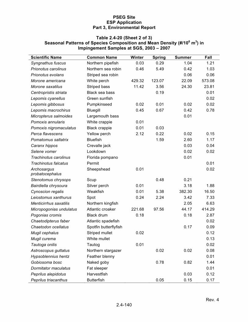
PSEG Site ESP Application
Part 3, Environmental Report
Rev. 4 2.4-140
Table 2.4-20 (Sheet 2 of 3) Seasonal Patterns of Species Composition and Mean Density (#/106 m3) in
Impingement Samples at SGS, 2003 – 2007 Scientific Name Common Name Winter Spring Summer Fall
Syngnathus fuscus Northern pipefish 0.03 0.29 1.04 1.21
Prionotus carolinus Northern sea robin 0.46 5.49 0.42 1.03
Prionotus evolans Striped sea robin 0.06 0.06
Morone americana White perch 429.32 123.07 22.09 573.08
Morone saxatilus Striped bass 11.42 3.56 24.30 23.81
Centropristis striata Black sea bass 0.19 0.01
Lepomis cyanellus Green sunfish 0.02
Lepomis gibbosus Pumpkinseed 0.02 0.01 0.02 0.02
Lepomis macrochirus Bluegill 0.45 0.67 0.42 0.78
Micropterus salmoides Largemouth bass 0.01
Pomoxis annularis White crappie 0.01
Pomoxis nigromaculatus Black crappie 0.01 0.03
Perca flavescens Yellow perch 2.12 0.22 0.02 0.15
Pomatomus saltatrix Bluefish 1.59 2.60 1.17
Caranx hippos Crevalle jack 0.03 0.04
Selene vomer Lookdown 0.02 0.02
Trachinotus carolinus Florida pompano 0.01
Trachinotus falcatus Permit 0.01
Archosargus probatocephalus
Sheepshead 0.01 0.02
Stenotomus chrysops Scup 0.48 0.21
Bairdiella chrysoura Silver perch 0.01 3.18 1.88
Cynoscion regalis Weakfish 0.01 5.38 382.30 16.50
Leiostomus xanthurus Spot 0.24 2.24 3.42 7.33
Menticirrhus saxatilis Northern kingfish 2.05 6.63
Micropogonias undulatus Atlantic croaker 221.68 97.56 44.17 414.29
Pogonias cromis Black drum 0.18 0.18 2.87
Chaetodipterus faber Atlantic spadefish 0.02
Chaetodon ocellatus Spotfin butterflyfish 0.17 0.09
Mugil cephalus Striped mullet 0.02 0.12
Mugil curema White mullet 0.13
Tautoga onilis Tautog 0.01 0.02
Astroscopus guttatus Northern stargazer 0.02 0.02 0.08
Hypsoblennius hentz Feather blenny 0.01
Gobiosoma bosc Naked goby 0.78 0.82 1.44
Dormitator maculatus Fat sleeper 0.01
Peprilus alepidotus Harvestfish 0.03 0.12
Peprilus triacanthus Butterfish 0.05 0.15 0.17

PSEG Site ESP Application
Part 3, Environmental Report
Rev. 4 2.4-141
Table 2.4-20 (Sheet 3 of 3) Seasonal Patterns of Species Composition and Mean Density (#/106 m3) in
Impingement Samples at SGS, 2003 – 2007
Scientific Name Common Name Winter Spring Summer Fall
Scomberomorus maculates Spanish mackerel 0.01
Etropus microstomus Smallmouth flounder
0.01 0.16 0.03 4.26
Paralichthys dentatus Summer flounder 0.05 2.30 0.93 0.36
Paralichthys oblongus Fourspot flounder 0.02
Scophthalmus aquosus Windowpane flounder
0.15 3.54 0.03
Pseudopleuronectes americanus
Winter flounder 0.37 0.35 0.02
Trinectes maculatus Hogchoker 2.60 45.06 36.22 35.73
Symphurus plagiusa Blackcheek tonguefish
0.03 0.03 0.01
Sphoeroides maculatus Northern puffer 0.01 0.02
Total density 776.30 483.27 561.84 1193.41
Number of species 46 53 57 62
References 2.4-159 through 2.4-163

PSEG Site ESP Application
Part 3, Environmental Report
Rev. 4 2.4-142
Table 2.4-21 (Sheet 1 of 3) Species Composition and Density (#/100 m3) in Entrainment Samples from SGS, 2003 – 2007
Name Egg Larva Juvenile Adult 2003 2004 2005 2006 2007 5-Year Mean
American eel X X X 0.12 0.06 0.21 0.12 0.18 0.1
Clupeidae X X 0.02 0.01 0.01 0.02 0.07 0.0
Alosa sp. X X 0.08 0.07 0.06 0.04 0.1
Blueback herring X X 0.01 0.03 0.01 0.01 0.01 0.0
Alewife X X 0.02 0.03 0.01 0.03 0.05 0.0
Atlantic menhaden X X X 0.20 0.47 1.06 5.02 1.47 1.6
Atlantic herring X 0.01 0.0
Bay anchovy X X X X 13.15 100.52 54.58 101.45 173.80 88.7
Cyprinidae X 0.01 0.01 0.01 0.23 0.01 0.1
Common carp X 0.01 0.01 0.01 0.0
Eastern silvery minnow X 0.01 0.0
Catostomidae X 0.01 0.01 0.0
Quillback carpsucker X 0.09 0.1
White sucker X 0.01 0.0
Channel catfish X 0.01 0.0
Inshore lizardfish X 0.01 0.0
Oyster toadfish X 0.01 0.0
Spotted hake X 0.01 0.01 0.01 0.01 0.0
Striped cusk-eel X X 0.01 0.01 0.01 0.0
Atlantic needlefish X X 0.01 0.01 0.01 0.0
Sheepshead minnow X 0.01 0.0
Fundulus sp. X 0.01 0.02 0.02 0.01 0.0
Banded killifish X X 0.01 0.01 0.0
Mummichog X X 0.01 0.01 0.01 0.02 0.01 0.0
Striped killifish X 0.01 0.0
Rough silverside X X 0.14 0.04 0.1

PSEG Site ESP Application
Part 3, Environmental Report
Rev. 4 2.4-143
Table 2.4-21 (Sheet 2 of 3) Species Composition and Density (#/100 m3) in Entrainment Samples from SGS, 2003 – 2007
Name Egg Larva Juvenile Adult 2003 2004 2005 2006 2007 5-Year Mean
Menidia sp. X X X X 0.01 0.10 0.12 2.25 0.28 0.6
Inland silverside X X X X 0.01 0.62 0.03 0.02 0.2
Atlantic silverside X X X X 0.15 0.47 0.55 0.28 0.12 0.3
Northern pipefish X X X 0.07 0.07 0.10 0.06 0.05 0.1
Northern sea robin X 0.01 0.0
Striped sea robinsea robin
X 0.01 0.0
Morone sp. X 0.87 0.44 0.40 0.11 10.69 2.5
White perch X X X 0.44 0.64 0.25 0.55 1.21 0.6
Striped bass X X X 5.07 1.84 4.02 0.54 42.34 10.8
Centrarchidae X 0.01 0.0
Bluegill X 0.01 0.0
Yellow perch X 0.02 0.01 0.01 0.01 0.02 0.0
Sciaenidae X 0.01 0.01 0.01 0.01 0.0
Silver perch X X X 0.02 0.03 0.02 0.0
Weakfish X X X 0.43 1.10 2.09 0.70 1.44 1.2
Spot X X 0.01 0.25 0.01 0.03 0.1
Northern kingfish X X 0.01 0.01 0.0
Atlantic croaker X X 2.63 5.05 5.56 10.51 5.88 5.9
Black drum X X 0.01 0.01 0.02 0.0
Tautog X 0.01 0.0
American sand lance X 0.01 0.0
Gobiosoma sp. X X 0.01 0.01 0.0
Naked goby X X X X 30.09 22.33 30.86 54.89 25.42 32.7
Green goby X X X 0.02 0.02 0.01 0.0
Smallmouth flounder X X 0.01 0.01 0.01 0.02 0.0
Summer flounder X X 0.08 0.06 0.01 0.12 0.11 0.1

PSEG Site ESP Application
Part 3, Environmental Report
Rev. 4 2.4-144
Table 2.4-21 (Sheet 3 of 3) Species Composition and Density (#/100 m3) in Entrainment Samples from SGS, 2003 – 2007
Name Egg Larva Juvenile Adult 2003 2004 2005 2006 2007 5-Year Mean
Windowpane X X 0.01 0.01 0.0
Winter flounder X X 0.01 0.02 0.02 0.02 0.0
Hogchoker X X 0.07 0.05 0.09 0.09 0.09 0.1
Blackcheek tonguefish X 0.01 0.0
Northern puffer X 0.01 0.0
Total density 53.7 133.5 101.1 177.5 263.5 146.2
Number of species 31 33 35 44 36 57
References 2.4-159 through 2.4-163

PSEG Site ESP Application
Part 3, Environmental Report
Rev. 4 2.4-145
Table 2.4-22 (Sheet 1 of 4) Seasonal Patterns of Species Composition and Mean Density (#/106 m3) in Entrainment Samples at SGS, 2003 – 2007
Common Name Winter Spring
Eggs Larvae Juvenile Adult Eggs Larvae Juvenile AdultAmerican eel 585.19 223.02 261.62 87.16Blueback herring 11.73 4.38 4.71Alewife 6.05 127.82 2.39Atlantic menhaden 6.05 53.92 4855.22 319.65 1008.00 4761.95Atlantic herring 6.05Bay anchovy 392.16 6.18 142,045.94 41,356.00 1089.24 440.00Common carp 4.79Silvery minnow 3.63White sucker Channel catfish Inshore lizardfish Oyster toadfish Spotted hake 5.95 18.15Striped cusk-eel 0.99 2.42Atlantic needlefish 0.99Sheepshead minnow 1.21Banded killifish 1.10Mummichog 6.69Striped killifish Rough silverside 95.95Inland silverside 2.89 544.61Atlantic silverside 9.07 14.43 64.61 845.11 48.05 14.47Northern pipefish 8.74 1.32 42.91 2.64Northern sea robin Striped sea robin White perch 68.60 1.21 2178.28 25.11Striped bass 182.29 50,717.97 452.70Bluegill Yellow perch 57.88

PSEG Site ESP Application
Part 3, Environmental Report
Rev. 4 2.4-146
Table 2.4-22 (Sheet 2 of 4) Seasonal Patterns of Species Composition and Mean Density (#/106 m3) in Entrainment Samples at SGS, 2003 – 2007
Common Name Winter Spring
Eggs Larvae Juvenile Adult Eggs Larvae Juvenile AdultSilver perch 1.21 1.21Weakfish 62.01 1200.04 423.45Spot 33.10 179.32Northern kingfish Atlantic croaker 3.02 18.04 9001.74 1.32 966.41Black drum 8.21Tautog 1.32American sand lance 6.94Naked goby 2.79 3.02 5.59 4.84 33,776.70 38.88 81.51Green goby 3.16Smallmouth flounder 0.99Summer flounder 93.78 277.61 5.88 30.27Windowpane flounder 7.01Winter flounder 20.53 8.81Hogchoker 2.97 5.61 1.10Blackcheek tonguefish Northern puffer 0.99 Total Density 9.07 753.72 14,871.93 32.25 142,776.50 132,188.06 8184.79 542.25Number of Species 2 5 14 5 8 28 21 6

PSEG Site ESP Application
Part 3, Environmental Report
Rev. 4 2.4-147
Table 2.4-22 (Sheet 3 of 4) Seasonal Patterns of Species Composition and Mean Density (#/106 m3) in Entrainment Samples at SGS, 2003 – 2007
Common Name Summer Fall
Eggs Larvae Juvenile Adult Eggs Larvae Juvenile AdultAmerican eel 3.44 26.61 1.68 11.62Blueback herring 38.69 10.66 45.62Alewife 241.80 6.53Atlantic menhaden 463.31 131.68 890.76 262.42Atlantic herring Bay anchovy 280,645.21 80,216.01 12,128.00 30.59 9.26 1662.27 2566.15 6.23Common carp 3.24Silvery minnow White sucker 1.62Channel catfish 1.62Inshore lizardfish 1.63Oyster toadfish 4.90Spotted hake Striped cusk-eel Atlantic needlefish 1.81 3.24Sheepshead minnow
Banded killifish 5.64Mummichog 13.31 1.68 20.47Striped killifish 1.62Rough silverside 117.15 1.81Inland silverside 5.05 70.09Atlantic silverside 10.13 621.45 54.12 57.90 2.92 25.21Northern pipefish 1.68 303.66 29.95 22.75 5.75Northern sea robin 1.63

PSEG Site ESP Application
Part 3, Environmental Report
Rev. 4 2.4-148
Table 2.4-22 (Sheet 4 of 4) Seasonal Patterns of Species Composition and Mean Density (#/106 m3) in Entrainment Samples at SGS, 2003 – 2007
Common Name Summer Fall
Eggs Larvae Juvenile Adult Eggs Larvae Juvenile AdultStriped sea robin 1.68White perch 1.62 849.55 125.91 136.15Striped bass 2513.81 1400.80 13.31Bluegill 4.44Yellow perch Silver perch 15.16 23.47 2.92Weakfish 530.00 2008.95 3056.87 35.50Spot 6.53 66.93 3.41Northern kingfish 1.81 3.24Atlantic croaker 1134.91 2504.82 2.92 4616.31 54,607.08Black drum 5.00 3.41Tautog 1.62American sand lance
Naked goby 51.49 179,031.12 1723.09 189.73 121.77 145.22 182.65Green goby 5.69 2.84Smallmouth flounder
4.86 1.68 2.92
Summer flounder 272.05 249.01Windowpane flounder
1.62
Winter flounder Hogchoker 471.25 6.75 4.44 12.57Blackcheek tonguefish
1.62 2.92
Northern puffer Total Density 281,360.65 267,725.88 21,591.20 311.66 12.18 7576.21 58,150.73 225.48Number of Species
7 27 24 6 2 8 20 5
References 2.4-159 through 2.4-163

PSEG Site ESP Application
Part 3, Environmental Report
Rev. 4 2.4-149
Table 2.4-23 (Sheet 1 of 4) Species Composition and Abundance in Fish Surveys of the Delaware River (River Miles 40 – 60) near the PSEG Site, 2003 – 2007
Scientific Name Common Name
2003 2004 Trawl
(Bottom) Trawl
(Pelagic) Seine Trawl
(Bottom) Trawl
Seine (Pelagic) Acipenser brevirostrum Shortnose sturgeon 1 Acipenser oxyrhinchus Atlantic sturgeon x Anguilla rostrata American eel 167 x 64 3 x Conger oceanicus Conger eel Hyporhamphus unifasciatus Halfbeak Alosa aestivalis Blueback herring 14 x 43 x Alosa pseudoharengus Alewife 30 22 x 3 42 x Alosa sapidissima American shad 5 x 7 x Brevoortia tyrannus Atlantic menhaden 22 x 22 x Clupea harengus Atlantic herring 1 22 Dorosoma cepedianum Gizzard shad x 1 x Anchoa hepsetus Striped anchovy 40 x 6 Anchoa mitchilli Bay anchovy 84 11,694 x 305 8568 x Cyprinus carpio Common carp x x Hybognathus regius Eastern silvery minnow x Ameiurus catus White catfish 3 x Ameiurus nebulosus Brown bullhead 1 1 Ictaluras punctatus Channel catfish 19 x 79 x Synodus foetans Inshore lizardfish Opsanus tau Oyster toadfish 81 12 Gobiesox strumosus Skilletfish Urophysis chuss Red hake 1 Urophysis regia Spotted hake 1019 87 232 Ophidion marginata Striped cusk-eel 155 3 14 1 Strongylura marina Atlantic needlefish 1 x 1 Cyprinodon variegatus Sheepshead minnow x Fundulus diaphanus Banded killifish x Fundulus heteroclitus Mummichog x x Fundulus luciae Spotfin killifish x Fundulus majalis Striped killifish x x Membras martinica Rough silverside Menidia beryllina Inland silverside Menidia menidia Atlantic silverside 24 x 2 x

PSEG Site ESP Application
Part 3, Environmental Report
Rev. 4 2.4-150
Table 2.4-23 (Sheet 2 of 4) Species Composition and Abundance in Fish Surveys of the Delaware River (River Miles 40 – 60) near the PSEG Site, 2003 – 2007
Scientific Name Common Name
2003 2004 Trawl
(Bottom) Trawl
(Pelagic) Seine Trawl
(Bottom) Trawl
Seine (Pelagic) Syngnathus fuscus Northern pipefish 1 6 x 6 x Prionotus carolinus Northern sea robin 9 1 2 1 Prionotus evolans Striped sea robin 1 Morone americana White perch 468 16 x 674 38 x Morone saxatilis Striped bass 126 27 x 56 7 x Centropristis striata Black sea bass 2 Enneacanthus gloriosus Bluespotted sunfish Lepomis macrochirus Bluegill x Micropterus salmoides Largemouth bass Etheostoma olmstedi Tessellated darter 1 Pomatomus saltatrix Bluefish 4 x 7 x Caranx hippos Crevalle jack Trachinotus carolinus Pompano Stenotomus chrysops Scup Bairdiella chrysoura Silver perch 1 Cynoscion regalis Weakfish 267 468 x 1707 546 x Leiostomus xanthurus Spot x Menticirrhus saxatilis Northern kingfish 1 29 Micropogonias undulatus Atlantic croaker 3260 6663 7626 8725 x Pogonias cromis Black drum x 1 x Chaetodipterus faber Atlantic spadefish Mugil curema White mullet x Astroscopus guttatus Northern stargazer 1 Chasmodes bosquianus Striped blenny Gobiosoma bosc Naked goby 87 27 17 40 Peprilus triacanthus Butterfish 3 Scomberomerus maculatus Spanish mackerel 1 x Etropus microstomus Smallmouth flounder 1 Paralichthys dentatus Summer flounder 1 2 x Scophthalmus aquosus Windowpane flounder 2 Pseudopleuronectes americanus Winter flounder 1 Trinectes maculatus Hogchoker 1192 17 x 1660 16 Symphurus plagiusa Blackcheek tonguefish
Total number of individuals 6972 19,166 12,492 18,087 Total number of species 21 23 27 23 23 24

PSEG Site ESP Application
Part 3, Environmental Report
Rev. 4 2.4-151
Table 2.4-23 (Sheet 3 of 4) Species Composition and Abundance in Fish Surveys of the Delaware River (River Miles 40 – 60) near the PSEG Site, 2003 – 2007
Scientific Name Common Name
2005 2006 2007 Trawl
Seine Trawl
(Bottom) Seine Trawl
(Bottom) Seine (Bottom) Acipenser brevirostrum Shortnose sturgeon Acipenser oxyrhinchus Atlantic sturgeon Anguilla rostrata American eel 93 x 70 x 46 x Conger oceanicus Conger eel 2 Hyporhamphus unifasciatus Halfbeak x Alosa aestivalis Blueback herring 6 x 2 x Alosa pseudoharengus Alewife 9 x 22 x Alosa sapidissima American shad x 1 x 1 x Brevoortia tyrannus Atlantic menhaden x 1 x x Clupea harengus Atlantic herring Dorosoma cepedianum Gizzard shad 2 x x x Anchoa hepsetus Striped anchovy x x x Anchoa mitchilli Bay anchovy 105 x 227 x 220 x Cyprinus carpio Common carp x x Hybognathus regius Eastern silvery minnow 2 1 Ameiurus catus White catfish 1 x 3 x 7 x Ameiurus nebulosus Brown bullhead x 2 Ictaluras punctatus Channel catfish 33 x 5 x 20 x Synodus foetans Inshore lizardfish x Opsanus tau Oyster toadfish 36 33 49 Gobiesox strumosus Skilletfish 1 Urophysis chuss Red hake 2 Urophysis regia Spotted hake 34 457 60 Ophidion marginata Striped cusk-eel 66 30 17 Strongylura marina Atlantic needlefish x Cyprinodon variegatus Sheepshead minnow Fundulus diaphanus Banded killifish Fundulus heteroclitus Mummichog x x x Fundulus luciae Spotfin killifish Fundulus majalis Striped killifish x x x Membras martinica Rough silverside x Menidia beryllina Inland silverside x Menidia menidia Atlantic silverside x x x Syngnathus fuscus Northern pipefish 7 1 4

PSEG Site ESP Application
Part 3, Environmental Report
Rev. 4 2.4-152
Table 2.4-23 (Sheet 4 of 4) Species Composition and Abundance in Fish Surveys of the Delaware River (River Miles 40 – 60) near the PSEG Site, 2003 – 2007
Scientific Name Common Name
2005 2006 2007 Trawl
Seine Trawl
(Bottom) Seine Trawl
(Bottom) Seine (Bottom) Prionotus carolinus Northern sea robin 3 9 9 Prionotus evolans Striped sea robin Morone americana White perch 470 x 243 x 435 x Morone saxatilis Striped bass 169 x 9 x 9 x Centropristis striata Black sea bass 2 12 Enneacanthus gloriosus Bluespotted sunfish x Lepomis macrochirus Bluegill Micropterus salmoides Largemouth bass x Etheostoma olmstedi Tessellated darter Pomatomus saltatrix Bluefish x x 2 x Caranx hippos Crevalle jack x x Trachinotus carolinus Pompano x Stenotomus chrysops Scup 1 5 Bairdiella chrysoura Silver perch 9 x 8 7 x Cynoscion regalis Weakfish 4497 x 682 x 845 x Leiostomus xanthurus Spot 147 x 1 x 29 x Menticirrhus saxatilis Northern kingfish 8 x 46 x 87 x Micropogonias undulatus Atlantic croaker 2001 x 3295 x 2948 x Pogonias cromis Black drum 9 x x 10 x Chaetodipterus faber Atlantic spadefish 3 Mugil curema White mullet x x Astroscopus guttatus Northern stargazer 1 6 Chasmodes bosquianus Striped blenny 1 Gobiosoma bosc Naked goby 21 2 2 Peprilus triacanthus Butterfish 1 Scomberomerus maculatus Spanish mackerel Etropus microstomus Smallmouth flounder 1 25 Paralichthys dentatus Summer flounder 4 x 1 4 x Scophthalmus aquosus Windowpane flounder 1 14 Pseudopleuronectes americanus Winter flounder 1 Trinectes maculatus Hogchoker 1854 1594 x 1221 x Symphurus plagiusa Blackcheek tonguefish 10 Total number of individuals 9590 6752 6110 Total number of species 28 29 30 25 31 28
x = present in collections from PSEG Beach Seine Program References 2.4-159 through 2.4-163
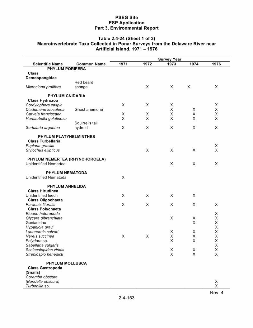
PSEG Site ESP Application
Part 3, Environmental Report
Rev. 4 2.4-153
Table 2.4-24 (Sheet 1 of 3) Macroinvertebrate Taxa Collected in Ponar Surveys from the Delaware River near
Artificial Island, 1971 – 1976
Scientific Name Common Name Survey Year
1971 1972 1973 1974 1976 PHYLUM PORIFERA
Class Demospongidae
Microciona prolifera Red beard sponge X X X X
PHYLUM CNIDARIA
Class Hydrozoa Cordylophora caspia X X X X Diadumene leucolena Ghost anemone X X X Garveia franciscana X X X X X Hartlaubella gelatinosa X X X X X
Sertularia argentea Squirrel's tail hydroid X X X X X
PHYLUM PLATYHELMINTHES
Class Turbellaria Euplana gracilis X Stylochus ellipticus X X X X PHYLUM NEMERTEA (RHYNCHOROELA)
Unidentified Nemertea X X X
PHYLUM NEMATODA Unidentified Nematoda X
PHYLUM ANNELIDA Class Hirudinea Unidentified leech X X X X Class Oligochaeta Paranais litoralis X X X X X Class Polychaeta Eteone heteropoda X Glycera dibranchiata X X X Goniadidae X X Hypaniola grayi X Laeonereis culveri X X X Nereis succinea X X X X X Polydora sp. X X X Sabellaria vulgaris X Scolecolepides viridis X X X Streblospio benedicti X X X
PHYLUM MOLLUSCA Class Gastropoda (Snails) Corambe obscura (Boridella obscura) X Turbonilla sp. X

PSEG Site ESP Application
Part 3, Environmental Report
Rev. 4 2.4-154
Table 2.4-24 (Sheet 2 of 3) Macroinvertebrate Taxa Collected in Ponar Surveys from the Delaware River near
Artificial Island, 1971 – 1976
Scientific Name Common Name Survey Year
1971 1972 1973 1974 1976 Class Pelecypoda Crassostrea virginica Eastern oyster X X X X X Macoma balthica Baltic macoma X X X X X
Macoma tenta Elongate macoma X
Modiolus demissus Ribbed mussel X X X X X Mulinia lateralis Dwarf surfclam X X Mya arenaria Soft-shell clam X Mytilopsis(Congeria leucophaeata) Dark falsemussel X X X X Rangea cuneata Common rangia X X X X X Macoma sp. X
PHYLUM ARTHROPODA Subphylum Chelicerata Class Arachnida Acarina Aquatic mites X Subphylum Crustacea Order Amphipoda (Scuds) Caprellidae X Corophium lacustre X X X X X Gammarus spp. X X X X X Leptocheirus plumulosis X X X X X Melita nitida X X X X Monoculodes edwardsi X X X Parahaustorius sp. X X X Parapleustes sp. X Order Cumacea (Hooded shrimps) Leucon americanus X X X X Order Decapoda Callinectes sapidus Blue crab X X Crangon septemspinoza Sand shrimp X X X X X
Palaemonetes pugio Daggerblade grass shrimp X X X X
Panopeus herbstii Atlantic mud crab X
Rhithropanopeus harrisii Estuarine mud crab X X X X X
Order Isopoda (Pill bugs, wood lice) Cassidinidea lunifrons X X X Chiridotea almyra X X X X X Cyathura polita X X X X X Edotea triloba X X X X X Order Mysidacea (Opossum shrimps) Mysidopsis bigelowi Neomysis americana X X X X X Order Thoracica Balanus improvisus Bay barnacle X X X X X

PSEG Site ESP Application
Part 3, Environmental Report
Rev. 4 2.4-155
Table 2.4-24 (Sheet 3 of 3) Macroinvertebrate Taxa Collected in Ponar Surveys from the Delaware River near
Artificial Island, 1971 – 1976
Scientific Name Common Name Survey Year(a)
1971 1972 1973 1974 1976 Subphylum Mandibulata Class Insecta Order Diptera Chironomidae Non-biting midges X X X X X Tipulidae Craneflies X X
PHYLUM BRYOZOA (ECTOPROCTA) Class Gymnolaemata Amathia vidovici X X X X X Membraniporidae X
PHYLUM CHORDATA Class Ascidiacea Molgula manhattensis Sea grape X X
Reference 2.4-25
a) No data reported for 1975.

PSEG Site ESP Application
Part 3, Environmental Report
Rev. 4 2.4-156
Table 2.4-25 Taxonomic Composition and Abundance in Macroinvertebrate Surveys Collected by
Ponar Dredge in the Delaware River near the PSEG Site, 2009(a)
Scientific Name
Spring Fall
AS-07 AS-12 AS-13 AS-15 AS-07 AS-12 AS-13 AS-15
PHYLUM ANNELIDA
Class Oligochaeta
Unidentified Enchytraeidae 1
Unidentified Naididae 1 1
Unidentified Oligochaeta 1
Class Polychaeta
Unidentified Polychaeta 2 5 15 Order Spionida (Spionids)
Marenzelleria viridis 9 21
PHYLUM MOLLUSCA
Class Pelecypoda
Mya arenaria 1
Rangea cuneata 1
PHYLUM ARTHROPODA
Subphylum Crustacea Order Amphipoda (Scuds)
Unidentified Amphipoda 1
Corophium lacustre 5
Corophium sp. 1
Gammarus sp. 2 6
Gammarus daiberi 3
Haustorius canadensis 1
Monoculodes edwardsi 4 1 12
Protohaustorius wigleyi 1 Order Isopoda (Pill bugs, wood lice)
Chiridotea almyra 7 10
Chiridotea sp. 6 2
Cyathura polita 2
Order Mysida (Mysids)
Neomysis americana 3 2
Total number of individuals 29 11 21 43 0 0 0 23
Total number of taxa 10 2 5 5 0 0 0 1
a) Information in this table collected as part of ESPA sampling program.

PSEG Site ESP Application
Part 3, Environmental Report
Rev. 4 2.4-157
Table 2.4-26 (Sheet 1 of 2) Important Aquatic Species Potentially Occurring
in the Vicinity of the PSEG Site
Scientific Name Common Name Rationale Invertebrates
Horseshoe crab Limulus polyphemus Commercial - NJ and DE Eastern oyster Crassostrea virginica Commercial - NJ and DE Northern quahog clam Mercenaria mercenaria Commercial - NJ and DE Blue crab Callinectes sapidus Commercial - NJ and DE
Fish Shortnose sturgeon Acipenser brevirostrum Endangered - federal Atlantic sturgeon Acipenser oxyrhynchus Endangered candidate – federal; Endangered
- DE American eel Anguilla rostrata Commercial/recreational - NJ and DE Conger eel Conger oceanicus Commercial - NJ and DE Blueback herring Alosa aestivalis Representative Important Species - NJPDES Alewife Alosa pseudoharengus Representative Important Species - NJPDES American shad Alosa sapidissima Commercial - NJ and DE Atlantic menhaden Brevoortia tyrannus Commercial - NJ and DE Bay anchovy Anchoa mitchilli Representative Important Species - NJPDES Channel catfish Ictaluras punctatus Commercial - DE; recreational - NJ and DE Silver hake Merluccius bilinearis Commercial - NJ Atlantic silverside Menidia menidia Representative Important Species - NJPDES Northern sea robin Prionotus carolinus Commercial - NJ; recreational - NJ and DE White perch Morone americana Commercial/recreational - NJ and DE Striped bass Morone saxatilis Commercial - DE; recreational - NJ and DE Black sea bass Centropristis striata Commercial/recreational - NJ and DE Bluefish Pomatomus saltatrix Commercial/recreational - NJ and DE Scup Stenotomus chrysops Commercial - NJ; recreational - NJ and DE Weakfish Cynoscion regalis Commercial/recreational - NJ and DE Spot Leiostomus xanthurus Commercial - NJ and DE; recreational - DE Northern kingfish Menticirrhus saxatilis Commercial/recreational - NJ and DE Atlantic croaker Micropogonias undulatus Commercial/recreational - NJ and DE Black drum Pogonias cromis Commercial/recreational - NJ and DE Butterfish Peprilus tricanthus Commercial - NJ and DE Summer flounder Paralichthys dentatus Commercial/recreational - NJ and DE Windowpane flounder Scophthalmus aquosus Commercial - NJ Winter flounder Pseudopleuronectes
americanus Commercial - NJ; recreational - NJ

PSEG Site ESP Application
Part 3, Environmental Report
Rev. 4 2.4-158
Table 2.4-26 (Sheet 2 of 2) Important Aquatic Species Potentially Occurring
in the Vicinity of the PSEG Site
Scientific Name Common Name Rationale
Other Vertebrates Atlantic loggerhead turtle Caretta caretta Threatened – federal; Endangered – NJ and
DE Atlantic green turtle Chelonia mydas Threatened – federal and NJ; Endangered –
DE Leatherback turtle Dermochelys coriacea Endangered – federal; Endangered – NJ
and DE Hawksbill turtle Eretmochelys imbricata Endangered – federal; Endangered – NJ
and DE Kemp's ridley turtle Lepidochelys kempii Endangered – federal; Endangered – NJ
and DE References 2.4-37, 2.4-129, and 2.4-13442
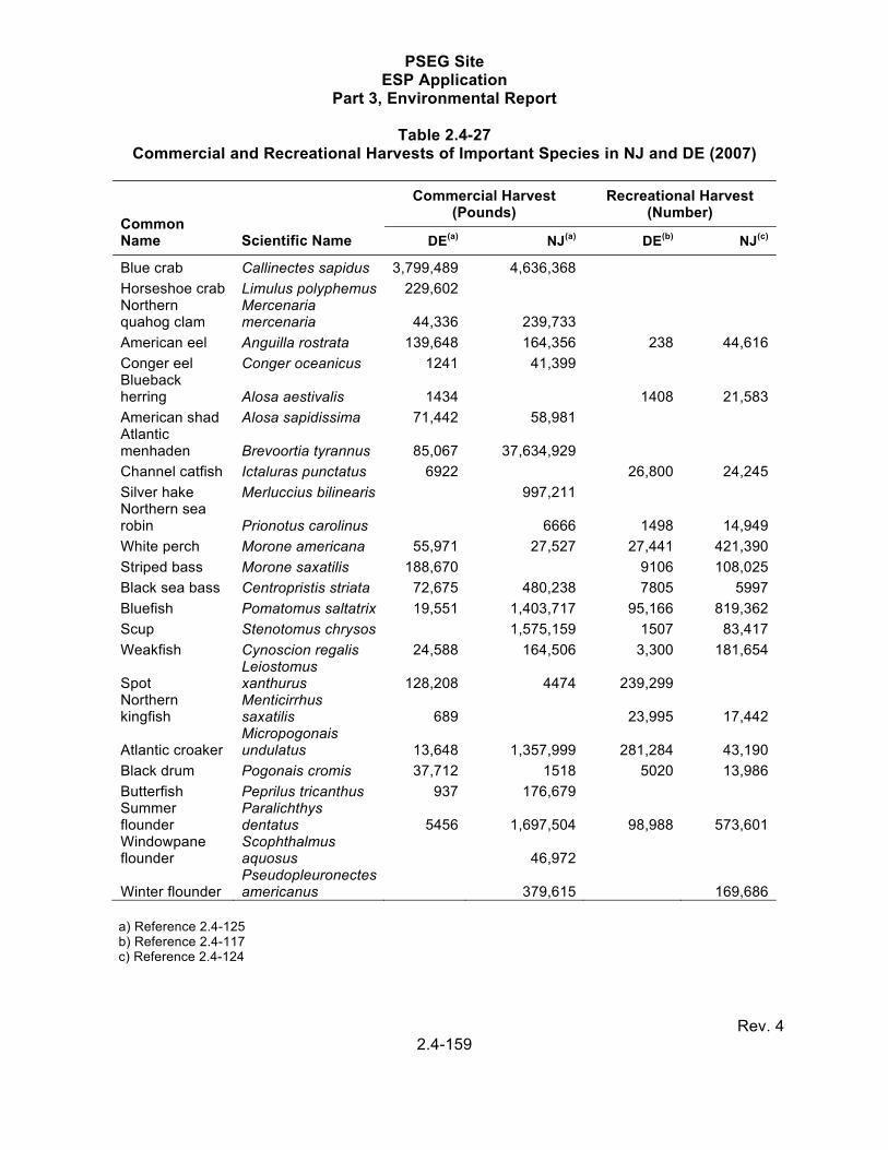
PSEG Site ESP Application
Part 3, Environmental Report
Rev. 4 2.4-159
Table 2.4-27 Commercial and Recreational Harvests of Important Species in NJ and DE (2007)
Common Name Scientific Name
Commercial Harvest (Pounds)
Recreational Harvest (Number)
DE(a) NJ(a) DE(b) NJ(c)
Blue crab Callinectes sapidus 3,799,489 4,636,368
Horseshoe crab Limulus polyphemus 229,602 Northern quahog clam
Mercenaria mercenaria 44,336 239,733
American eel Anguilla rostrata 139,648 164,356 238 44,616
Conger eel Conger oceanicus 1241 41,399 Blueback herring Alosa aestivalis 1434 1408 21,583
American shad Alosa sapidissima 71,442 58,981 Atlantic menhaden Brevoortia tyrannus 85,067 37,634,929
Channel catfish Ictaluras punctatus 6922 26,800 24,245
Silver hake Merluccius bilinearis 997,211 Northern sea robin Prionotus carolinus 6666 1498 14,949
White perch Morone americana 55,971 27,527 27,441 421,390
Striped bass Morone saxatilis 188,670 9106 108,025
Black sea bass Centropristis striata 72,675 480,238 7805 5997
Bluefish Pomatomus saltatrix 19,551 1,403,717 95,166 819,362
Scup Stenotomus chrysos 1,575,159 1507 83,417
Weakfish Cynoscion regalis 24,588 164,506 3,300 181,654
Spot Leiostomus xanthurus 128,208 4474 239,299
Northern kingfish
Menticirrhus saxatilis 689 23,995 17,442
Atlantic croaker Micropogonais undulatus 13,648 1,357,999 281,284 43,190
Black drum Pogonais cromis 37,712 1518 5020 13,986
Butterfish Peprilus tricanthus 937 176,679 Summer flounder
Paralichthys dentatus 5456 1,697,504 98,988 573,601
Windowpane flounder
Scophthalmus aquosus 46,972
Winter flounder Pseudopleuronectes americanus 379,615 169,686
a) Reference 2.4-125 b) Reference 2.4-117 c) Reference 2.4-124

PSEG Site ESP Application
Part 3, Environmental Report
Rev. 4 2.4-160
Table 2.4-28 EFH for Relevant Federally Managed Species in the Vicinity of the PSEG Site
Scientific Name Common Name Egg Larva Juvenile Adult
Prepilus triacanthus Butterfish X
Scophthalmus aquosus Windowpane flounder
X X X X
Pleuronectes americanus Winter flounder X X X X
Paralicthys dentatus Summer flounder X X

PSEG Site ESP Application
Part 3, Environmental Report
Rev. 4 2.4-161
Table 2.4-29
Stream Length (miles) within Each Potential Off-Site Transmission Macro-Corridor
South Corridor(a)
5-Mi. Wide Corridor
6-Mile Vicinity 6-50+ Mile
Region Total Channelized Waterway 197.3 431.2 628.5 Intermittent Stream 0.2 130.0 130.2 Perennial Stream 320.4 617.6 938.0
Total 518.0 1178.8 1696.7 West Corridorb Channelized Waterway 140.0 184.0 324.1 Intermittent Stream 0.0 79.7 79.7 Perennial Stream 236.0 330.3 566.3
Total 376.0 594.0 970.1
a) Total length = 94 mi. b) Total length = 55 mi.

PSEG Site ESP Application
Part 3, Environmental Report
Rev. 4 2.5-1
2.5 SOCIOECONOMICS This section characterizes the current socioeconomic resources within the 50-mi. region surrounding the PSEG Site. It provides the basis for assessing potential impacts to these resources as a result of the construction and operation of the new plant at the PSEG Site. The socioeconomic resources characterized are demographics, community characteristics, historic properties, and populations potentially subject to environmental justice considerations. The characterization of socioeconomic resources is presented on a spatial and temporal (demography) basis. The larger geographic area of analysis is a circular region extending 50 mi. from the center point of the new plant. Socioeconomic resources are also characterized for the 10-mi. vicinity, the 5-mi. low population zone (LPZ), and the exclusion area as required by NUREG-1555, Standard Review Plans for Environmental Reviews of Nuclear Power Plants: Environmental Standard Review Plan. For purposes of socioeconomic analysis, it is assumed that the residential distribution of the new plant construction and operational workforce resembles the residential distribution of the current workforce for HCGS and SGS, as shown in Table 2.5-1. Approximately 96.8 percent of the current workforce of the existing plants resides within nine counties in four states. Five of these counties are in NJ and include Salem (41.0 percent), Gloucester (14.6 percent), Cumberland (10.0 percent), Camden (3.6 percent), and Burlington (2.4 percent). Two PA counties are Chester (3.6 percent) and Delaware (2.5 percent). The remaining two counties are New Castle, DE (17.0 percent) and Cecil, MD (2.1 percent). The remaining 3.2 percent of the workforce resides in 22 other counties and five other states, with one to nine employees (0.1 to 0.6 percent of the existing workforce) per county. A total of 82.6 percent of the operational workforce for SGS and HCGS resides in Salem, Gloucester, and Cumberland counties in NJ, and New Castle County, DE. The construction and operational workforce of the new plant is assumed to have the same distribution. Therefore, these four counties represent the socioeconomic Region of Influence and serve as the basis for assessment of potential project effects from construction and operation. 2.5.1 DEMOGRAPHY The demography within the vicinity and region of the PSEG Site is characterized in the following subsections. This characterization includes a description of the resident and transient population distribution from 0 to 10 mi. and the resident population distribution from 10 to 50 mi. for: 2000, the resident populations from the U.S. Census Bureau (USCB) census 2010, the year of application submittal 2021, the first year of operation 2031 to 2081, the life of the plant at 10-yr increments This section also provides a description of resident population characteristics within the 0 to 10 mi. vicinity, the nearest special facilities and population centers, the 0 to 5 mi. LPZ, and the population densities within 20 mi. and 50 mi. of the site. As shown in Table 2.5-2, the 0 to 10 mi. vicinity includes parts of the four county Region of Influence in DE and NJ. The 10 to 50 mi. area includes parts or all of an additional 21 counties within DE, MD, NJ, and PA. Twenty-

PSEG Site ESP Application
Part 3, Environmental Report
Rev. 4 2.5-2
five counties, in four states, fall within 0 to 50 mi. of the PSEG Site, including all three counties in DE, seven counties each in MD and NJ, and eight counties in PA. Using USCB 2000 census block data (Reference 2.5-124), population estimates are developed for concentric circles divided into 22.5 degree sectors extending in intervals from 0 to 1 mi., 1 to 2 mi., 2 to 3 mi., 3 to 4 mi., 4 to 5 mi., 5 to 10 mi., 10 to 20 mi., 20 to 30 mi., 30 to 40 mi., and 40 to 50 mi. These intervals and sectors for the 0 to 10 mi. and 10 to 50 mi. areas are shown in Figures 2.5-1 and 2.5-2, respectively. For each sector grid, the percentage of each census block’s land area that fall within that sector, is calculated using the GIS software ArcMap 9.2. The equivalent proportion of each census block’s population is assigned to each sector grid. If portions of two or more census blocks fall within the same sector grid, the proportional population estimates for each census block are summed to obtain the population estimate. Population projections for 2010 are derived from the net change between the 2000 USCB population data and the 2008 USCB population estimates for each county. This net change over the eight-year period was extrapolated for an additional two years to derive the 2010 county population projections. The difference between the 2000 USCB population data and the derived 2010 population projection was used to determine the overall rate of change for each county. These rates of change were applied to the USCB 2000 census block data to obtain estimates of population change and distribution by sector and grid. Within the 0 to 10 mi. radius, USCB 2000 local population data and USCB 2007 local population estimates were used to refine 2010 projected populations, using the methodology described in the previous paragraph. These local rates of changes were used to modify the census block data within the 0 to 10 mi. radius. The 2010 county level projections were held constant for the remaining portion of the county that fell outside the 0 to 10 mi. radius, and the rate of change for this portion of the county was adjusted proportionately. The developed population baseline for 2010, which includes the redistributed local populations, is used to develop projections for 2021 and 2031. Using USCB census data and estimates, DE, MD, NJ, and PA have published population projections out to 2025 (NJ) and 2030 (DE, MD, and PA) at the county level (References 2.5-27, 2.5-60, 2.5-76, 2.5-89). The 2010 populations are determined by using the USCB growth rates for the 2000 through 2008 period (Reference 2.5-121). From 2010 onward, the growth rates are derived from published county population projections for each of the four states. These derived growth rates are used to extrapolate the baseline 2010 estimates out to 2021 and 2031 for each county within each state. No published data is available beyond the 2031 projections. Population projections beyond 2031 are based on the county-specific annual growth rate calculated for each county between 2021 and 2031. The county-specific growth rates for this 10-yr period are used to develop the population projections for each successive 10-yr period (2041, 2051, 2061, 2071 and 2081).

PSEG Site ESP Application
Part 3, Environmental Report
Rev. 4 2.5-3
2.5.1.1 Current and Projected Population Levels 2.5.1.1.1 Resident Population Distribution within 0 to 10 Miles Figure 2.5-1 shows a 10-mi. radius sector chart from the center point for the new plant location, which is north (N) of and adjacent to HCGS. A total of 96 individual sectors are included in the 0 to 10 mi. area. Resident population data are calculated for each of the 96 sectors. The resultant population distributions are summarized in Table 2.5-3 by distance and year. Based on 2000 USCB census data, 33,871 people reside within 10 miles of the new plant. Approximately 94 percent of the population resides in the 5 to 10 mi. area. There is no resident population within 2 mi. of the PSEG Site. An estimated 75 individuals reside within 2 to 3 mi. of the site. The most densely populated sectors are the west-southwest (WSW), west (W), west-northwest (WNW) and northwest (NW) sectors located in DE, with a combined population of 17,690 residents. The north-northeast (NNE), northeast (NE), east-northeast (ENE), and east (E) sectors in NJ have a combined population of 11,351 residents. The nearest residence to the PSEG Site is approximately 2.8 mi. west in DE. The closest residences in Salem County are more than 3 mi. from the PSEG Site. The three largest communities in the 10-mi. vicinity, based on USCB 2007 population estimates, are Middletown, DE (11,153), Pennsville Township, NJ (13,363), and Salem, NJ (5678) (Table 2.5-4). Lower Alloways Creek and Elsinboro Townships are the NJ townships nearest to the PSEG Site with 2007 estimated populations of 1883 and 1054, respectively. Hancocks Bridge is nearest community and is located 5 mi. east of the PSEG Site in Lower Alloways Creek Township. A comparison of the Census 2000 data and 2007 estimates indicates that Middletown grew over the 7-yr period at an average rate of 8.8 percent per year, as compared to an average rate of only 0.7 percent per year (2000 to 2008) for all of New Castle County, DE. Salem City, NJ experienced an average rate of decline of 0.4 percent per year over this 7-yr period, while Salem County grew at an average rate of 0.4 percent per year. Cumberland County grew at an annual rate of 0.9 percent. Using the population projection methodology described in Subsection 2.5.1 to determine the 2010 to 2081 projected populations, the population within 10 mi. of the PSEG Site is projected to increase from 33,871 in 2000 to 42,743 in 2010 (Table 2.5-3). This represents an annual rate of growth of 2.35 percent per year, primarily due to the rapid growth in the Middletown-Odessa-Townsend, DE area. The population is projected to reach 45,527 in 2021 and 60,892 by the end of the new plant operation (2081). 2.5.1.1.2 Transient Population Distribution within 0 to 10 Miles In addition to the permanent resident population within 10 mi. of the PSEG Site, there are transient populations comprised of people that do not live within the 10-mi area but enter this area on a routine basis for employment, education (schools and daycare), recreation (parks, wildlife areas, resorts, beaches, lodging, and restaurants), and medical care (hospitals and assisted living). These transient populations are shown in Table 2.5-5, based primarily on surveys conducted in 2009 (Reference 2.5-44). Inmates at correctional facilities are considered to be transients, but there are no such facilities within a 10-mi. radius of the PSEG Site (Reference 2.5-44).

PSEG Site ESP Application
Part 3, Environmental Report
Rev. 4 2.5-4
The 2008 transient population within the 10-mi. area is estimated to be 12,085, with the majority of the transient population occurring within 5 to 10 mi. of the PSEG Site. Assuming the transient population grows at the same rate as the resident population, the transient population within 10 mi. is projected to increase to 12,549 in 2010, 13,378 in 2021, and 18,063 in 2081. Approximately 97.8 percent of the transient population within 10 miles of the PSEG Site is located between 5 and 10 mi. away and no individuals are less than 3 mi. from the PSEG Site. No transient facilities are within 3 mi. of the PSEG Site, however occasional recreational users and hunters visit portions of the Mad Horse Creek WMA in NJ, the Delaware River, adjoining coastal marsh systems, and the Cedar Swamp and Augustine WMAs in DE that fall within this 3-mi. radius. The main access points for these three WMAs fall outside the 3-mi. area. The daily usage data collected at these points provides the best estimates of where the major usage occurs, because there is limited land access to areas beyond the main access points. Transients in the 10-mi. area are primarily school students, tourists, employees (other than those at SGS and HCGS), and people undergoing medical care. As shown in Table 2.5-6, 66 percent of the transient population is located in DE and 34 percent in NJ. The transient population in NJ is concentrated in the NNE sector, and in the NNW to WSW sectors in DE. Students attending schools within the area comprise 34 percent of the transients. Visitors and tourists at local resorts, beaches, wildlife areas, parks, and marinas make up 26 percent of the transient population. Employees commuting to work represent another 34 percent of the transients, while people seeking medical care represent the smallest component of the transient population, at 5 percent. An undetermined portion of the transient population is double counted as they may reside in the 10 mile area surrounding the site. A survey was performed to collect information on the number of people per household and number of school age children per household within the 10-mi. vicinity. Based on this information, it is estimated that 72.7 percent of the students attending schools within the 10-mi. area are residents. Therefore, the number of students counted as transients in Table 2.5-6 represents 27.3 percent of all students attending schools within the 10-mi. vicinity. There are a number of influences on the future size and distribution of transient populations. For example, a large new employer locating in the area could dramatically increase the number of transient employees. Conversely, consolidation of several small schools into a single larger facility could increase or decrease this population based on the choice of location (for example, 9 mi. versus 11 mi. from the center point), and the area that the school serves. 2.5.1.1.3 Resident Population Distribution within 10 to 50 Miles Sixty-four sectors fall within the 10- to 50-mile area from the PSEG Site as indicated in Figure 2.5-2. Population data are calculated for each of the sectors. The resultant population distributions are summarized in Table 2.5-7 by distance and year. Based on Census 2000 data, an estimated 5,230,454 residents are located within 50 mi. of the PSEG Site; 5,196,583 people reside within 10 to 50 mi. Less than 1 percent of the regional population resides within 10 mi. of the site.

PSEG Site ESP Application
Part 3, Environmental Report
Rev. 4 2.5-5
Populations within 10 to 20, 20 to 30, 30 to 40 and 40 to 50 mi. represent 9.5, 12.7, 35.2, and 42.0 percent of the regional population, respectively. 10.1 and 22.8 percent of the regional population are within 20 and 30 mi. of the PSEG Site, respectively, while over 77 percent is within 30 to 50 mi. Over 70 percent of the 10 to 50 mi. population resides in the N, NNE, or NE sectors. This distribution corresponds with the location of the primary population centers in the region. The three largest population centers within the region are Philadelphia in the NNE (1,517,550), Camden in the NE (79,904), and Wilmington in the N (72,664). Based on the population projection methodology described in Subsection 2.5.1, the areas within 10 to 20 mi. and 20 to 30 mi. of the PSEG Site center point have 2000 to 2010 average annual growth rates of 0.8 and 1.1 percent, respectively. This is more than double the 0.4 percent annual growth rate within 30 to 40 mi. The area within 40 to 50 mi. of the PSEG Site had the lowest average annual growth rate at 0.2 percent. The Philadelphia metropolitan area falls in this 30 to 50 mi. area and accounts for the majority of its population. Table 2.5-7 shows that projected population levels within the 50-mi. region increase to 5,806,512 at the projected construction completion date (2021) for the new plant and increase to 8,138,635 by the end of the plant life (2081). Within 10 to 20 mi. of the plant, the population is projected to increase from 2010 to 2021 from 535,164 to 579,362, and from 535,164 to 828,052 in 2081. The greatest increase in population is in the 20 to 30 mi. area with projected populations of 737,825 in 2010, 811,029in 2021, and 1,321,698 in 2081. The lowest projected population growth is 40 to 50 mi. from the PSEG Site where populations are projected as 2,237,530 in 2010 and 2,346,225 in 2021, and 3,024,126 in 2081. 2.5.1.1.4 Complete Distribution and Projection of the Resident Population Table 2.5-8 shows the distribution and projection of the resident population for all 16 sectors and distances from 2000 to 2081. The most populated sectors are the NNE, NE and N, while the least populated sectors are the south-southeast (SSE), southwest (SW), and southeast (SE). Based on 2010 population projections, the NNE sector contains 37.5 percent (2,045,463) of the total population (5,460,955) within 50 mi. of the PSEG Site, the NE sector 18.9 percent (1,034,261), and the N sector 11.5 percent (626,269). The SSE, SW, and SE sectors each contain less than one percent, and cumulatively 1.4 percent (77,966), of the total population within the 50-mi. region. 2.5.1.2 Population Data by Political Jurisdiction All or parts of 25 counties are located within 50 mi. of the PSEG Site (Figure 2.5-2). As in Section 2.5, Cumberland, Gloucester, and Salem counties in NJ, and New Castle County in DE, are the four counties most affected by the construction and operation of a new plant at the PSEG Site. Portions of Cumberland, Salem and New Castle counties account for all of the area within 10 mi. of the PSEG site (Figure 2.5-1). As presented in Table 2.5-9, growth rates in Salem County were lower than the other counties and typically lower than statewide averages in both NJ and DE. While Salem County had a 7.2 percent population increase from 1970 to 1980, the county experienced negative growth in the decade from 1990 to 2000 (from 65,294 to 64,285). More recent data indicates that the population has increased to 66,141 (2.9 percent increase) from the years 2000 to 2008. By comparison, the growth rates of Gloucester, Cumberland and New Castle counties were higher over similar time periods. Overall, Gloucester County has experienced the highest rate of growth in the Region of Influence.

PSEG Site ESP Application
Part 3, Environmental Report
Rev. 4 2.5-6
All or part of the following jurisdictions (other than counties) are located within 10 mi. of the PSEG Site: Salem City, Lower Alloways Creek Township, Elsinboro Township, Pennsville Township, Quinton Township, Stow Creek Township, and Greenwich Township (all within NJ); and Delaware City, Middletown, Odessa, and Townsend (all within DE), as well as unincorporated areas of New Castle County in Delaware. Table 2.5-9 shows the USCB populations for these political jurisdictions for 1970, 1980, 1990, 2000, and 2007 to 2008. These data indicate that the population of Salem City, NJ has steadily declined from 7648 in 1970 to 5678 in 2007 (a decline of 26 percent). By contrast, the population of Middletown, DE has increased by 191 percent, from 3834 to 11,153 (between the years 1990 to 2007). Between these extremes, most of the other jurisdictions exhibit slow rates of change, often fluctuating between small gains and losses of population from decade to decade. 2.5.1.2.1 Characteristics of the Resident Population Table 2.5-10 presents demographic profiles from USCB 2000 for the counties and local jurisdictions presented in Table 2.5-9. County and state 2000 census information is also updated with information from the USCB 2005 – 2007 American Community Survey (ACS) 3-yr estimates for NJ, DE, and the four counties representing the socioeconomic Region of Influence. These profiles describe social structure characteristics such as gender, age, racial make-up, income, poverty levels, educational attainment, and housing characteristics for the four counties; and selected local communities within these counties that are likely to be affected by the construction and operation of a new plant. 2.5.1.2.1.1 New Jersey Comparing USCB 2000 averages for the counties within 10 mi. and NJ, Cumberland County has the lowest per capita income ($17,376), lowest levels of educational attainment, lowest median home values ($91,200) and the highest percentages of families and individuals living below the poverty line (11.3 percent). The racial profile exhibits the lowest percentage of whites (65.9 percent) and the highest percentage of Blacks (20.2 percent). The county also exhibits the highest ratio of Hispanics (19.0 percent), an ethnic category that is enumerated independently of racial identity. Compared to the other counties, Cumberland has more foreign born individuals and more households in which a language other than English is spoken. These numbers (foreign born and foreign language household) are below NJ state averages. In common with the other counties, Cumberland County has low numbers of Asians, as well as all other racial categories. The median age of the population is younger than the other counties. It is the only county in the four-county Region of Influence in which males are a majority of the population. The large and growing Hispanic population may be the most distinctive element of the demographic profile for this county. Gloucester County has the highest percentage of whites (87.1 percent), highest incomes ($22,708), home values ($120,100), levels of educational attainment, and home ownership in the four-county Region of Influence. The per capita income in USCB 2000 is approximately 84 percent of the NJ average, and the county exhibits lower levels of families and individuals living below the poverty line (4.3 percent, versus 11.3 and 7.2 percent for Cumberland and Salem Counties, respectively). Salem County falls between Cumberland and Gloucester Counties on most of the demographic profile items. Based on USCB 2000 data, the population of Salem County is

PSEG Site ESP Application
Part 3, Environmental Report
Rev. 4 2.5-7
older (median age 38.0) than the other counties in the four-county Region of Influence, as well as the state (36.7) or national (35.3) averages. The per capita income is $20,874 which is lower than the state average. The numbers of families and individuals living below the poverty line are higher than state averages. High school graduation rates in Salem County are close to the state average, but attainment of a college degree is slightly more than half of the state average. Owner-occupied housing in Salem County is 73 percent, which is higher than the state average (65.6 percent). The amount of vacant housing in Salem County (7.1 percent) is approximately the same as the state average (7.4 percent). The white population and the black population in Salem County are both higher than the state averages. Asian and Hispanic populations are below the state averages. Foreign-born residents make up 2.5 percent of the county population, compared to 17.5 percent of NJ’s population. Only 6.3 percent of Salem County households speak a language other than English at home, compared to a state average of 25.5 percent. Within Salem County, the largest concentrations of black populations and people living below the poverty level reside in Salem City. USCB 2000 reports that 56.8 percent of Salem City residents are black, and that 24.7 percent of families, and 26.6 percent of individuals live below the poverty line. The population is younger than the county average, with a median age of 33.5, compared to 38.0 for the county. People 18 yr and older total 69.0 percent in the city compared to 74.4 percent in the county. However, the population 65 yr and over is approximately the same for the city and the county. Males comprise 44.6 percent of the population. The per capita income of Salem City residents is $13,559. This is lower than the county ($20,874) and state averages ($27,006). Compared to county and state averages, fewer Salem City residents have completed high school or college and fewer people live in owner-occupied housing (41 percent versus 73 percent for the county). The value of owner-occupied housing is lower than the county average ($74,300 versus $105,200) while the percentage of vacant housing is more than twice the county average (16.8 percent versus 7.1 percent). Quinton Township is the only other local jurisdiction in the NJ portion of the study area with a per capita income ($18,921) below the Salem County average. It is also below the county average for educational attainment. More families and fewer individuals live below the poverty level. Quinton is above average for percent of owner-occupied housing (84 percent versus 73 percent for the county) and has a smaller percentage of vacant housing (5.2 percent versus 7.1 percent for the county). Its racial profile is similar to county averages, while the median age of the population is 1 year over the Salem County average. Economic and housing indicators for Elsinboro, Lower Alloways Creek and Pennsville townships are generally above Salem County averages, with Elsinboro generally scoring higher than the other townships. Families or individuals living in poverty range from 2 percent in Elsinboro Township to 4 percent in Lower Alloways Creek Township. Elsinboro has the highest owner-occupied housing, but also has more than twice the vacant housing units. Educational attainment for the three localities is similar to the county average. The number of racial minorities in all three townships is low; over 95 percent of the population in these localities is white, compared to the county average of 81.2 percent. The gender profiles are generally similar to the Salem County profile, but the median age of the Elsinboro population

PSEG Site ESP Application
Part 3, Environmental Report
Rev. 4 2.5-8
is 5.6 yr older than the county average, while the median age for the other two townships is 1.3 to 1.5 yr over the county average. A small portion of Stow Creek and Greenwich townships fall within the 10-mi. area. These townships have higher median ages (40.7 and 43.4, respectively), educational attainment, percentage of owner-occupied homes (87.9 percent and 86.2 percent, respectively), and median home values ($114,400 and $112,000, respectively) than the other NJ political jurisdictions. The populations in these two townships are predominantly white (93.4 percent and 90.0 percent, respectively). A small percent (5.7 percent and 6.1 percent, respectively) of the families are below poverty level. 2.5.1.2.1.2 Delaware In DE, New Castle County accounts for approximately 64 percent of the total state 2000 population, which results in little differentiation in the demographic profiles between the county and state. In the areas within 10 mi. of the PSEG Site, demographic profiles are available for four municipalities, two of which represent populations of less than 500 persons each. Much of the population in this area resides in unincorporated areas for which specific demographic profiles are not available. Middletown is the largest municipality in the area within 10 mi. of the PSEG Site. Middletown has a residential population that increased markedly from 3834 in 1990 to 11,153 in 2007 (Table 2.5-9). The population of the town was reported as 6161 in USCB 2000. At that time, the community exhibited a 4.8 percent gender gap. It also had the highest percentage of population under 5 yr of age (9.3 percent), the lowest over 65 years (7.9 percent) and the youngest median age (30.9 yr) of any jurisdiction in the vicinity. The racial distribution was similar to the county average; 74.4 percent white and 21.3 percent black. Per capita income was below the county average. Families and individuals living below the poverty level were highest among the DE municipalities within 10 mi. of the PSEG Site, and educational attainment was the lowest. Median home values and percent vacant housing ranked in the middle of the range of DE municipalities in the vicinity, while percent owner-occupied was the lowest. The oldest and wealthiest municipality was the small community of Odessa (population 286 in 2000) (Table 2.5-9), with 17.8 percent over 65 yr, and a median age of 42. Odessa had the highest percentage of whites and lowest percentage of all minorities. Per capita income was highest among the DE municipalities within 10 mi. of the PSEG Site and the only municipality higher than the county average. No families, and 3.2 percent of individuals, lived below the poverty level. Household and family sizes were among the smallest in the study area, and educational attainment was the highest. Percent owner-occupied housing was average for the DE municipalities within 10 mi. of the PSEG Site, median home value was highest, and percent vacancy was lowest. Delaware City, and the small community of Townsend, in comparison to the averages for New Castle County, have more whites, half as many blacks, and fewer other races, foreign born, or households that speak a foreign language at home. Both have per capita incomes below the county average. Delaware City has an average number of families and individuals living in poverty; Townsend has far fewer. High school attainment is slightly below average, but college graduation rates are less than half the county average. Owner-occupied housing is

PSEG Site ESP Application
Part 3, Environmental Report
Rev. 4 2.5-9
above the county average while the median value of those homes is well below the county average. 2.5.1.3 Low Population Zone The LPZ for the new plant is the area within 5 mi. of the new plant center point (Reference 2.5-133) and is illustrated in Figure 2.5-3. This area is dominated by the open waters of Delaware River and Bay and the low coastal wetlands to the east and west of the PSEG Site. Much of these coastal wetlands are state owned and managed as wildlife areas and are protected from future development. Most of the land within 2 mi. of the PSEG Site in NJ is owned by PSEG, NJDEP or by the USACE. The majority of the privately owned land within this LPZ is managed for agricultural production and private access hunting and fishing. A total of 1929 people resided within the LPZ as of USCB 2000 (Figure 2.5-3). Two sectors (W and WNW) have a combined population of 877 (45.5 percent of LPZ total). The most populated sector in NJ was the ENE sector, with a total of 229 residents (11.9 percent) within the LPZ. The population within the LPZ is projected to grow to 2047, 2178, and 2903 by the years 2010, 2021, and 2081, respectively (Table 2.5-3). 2.5.1.4 Special Facilities and Population Centers 2.5.1.4.1 Special Facilities Ninety-six special facilities were identified within the 10-mi. radius of the PSEG Site. These special facilities include schools and daycare centers, employers, parks and recreation areas, medical and assisted-living facilities, and lodgings where people may have to be evacuated by responsible officials during an emergency. Table 2.5-11 lists the schools and daycare centers, their sectors, and approximate distance from the PSEG Site. Table 2.5-12 lists additional employment locations including medical and assisted-living facilities. Table 2.5-13 lists parks and recreation areas, and lodging. As shown in Table 2.5-11, a total of 39 schools and daycare centers are located within the 10-mi. radius of the PSEG Site. Twenty-four of these educational facilities are located in DE and 15 are in NJ. Twenty-one of these schools and daycare centers are between 8 and 10 mi. from the PSEG Site, five are less than 7 mi., and one is less than 5 mi. from the PSEG Site. In NJ, the majority (nine) of the schools and daycare centers are to the NNE, at distances varying from 5.4 to 9.0 mi. In DE, the schools and daycare centers are fairly evenly distributed between the WSW, W, WNW, and NW sectors. Twenty-two of these special facilities are located in DE between 8 and 10 mi. from the center point of the PSEG Site and 10 are located between 7 and 10 mi. from the site. School enrollments range from a low of 4 students to a high of over 1700. While PSEG’s HCGS and SGS are major employers (1574 employees), they are not considered special facilities. Excluding HCGS and SGS, a total of 28 employers are located within the vicinity; 15 in DE and 13 in NJ (Table 2.5-12). The highest concentration of employers occurs in the NNW and W sectors of DE, with most located between 9.6 to 9.9 mi. from the PSEG Site. The remaining businesses are 7.2 to 8.9 mi. away. Twelve of the businesses in NJ are located in the NNE sector at a distance of 6.9 to 9.1 mi. and one in the ENE sector at a distance of 5.9 mi. Employee estimates range from 3 to 720 for businesses

PSEG Site ESP Application
Part 3, Environmental Report
Rev. 4 2.5-10
in this area, with Valero Oil Refinery (600) in Delaware City, Mannington Mills (550) in Salem City, Memorial Hospital (720) in Salem City, and the Office of Salem County (491) in Salem City, being the largest employers. The Valero Oil Refinery closed in late 2009. The final disposition of the refinery, including the potential for sale and/or reopening is not currently known. All the remaining businesses have from 3 to 150 employees. (Reference 2.5-44) As indicated in Table 2.5-13, there are 27 parks and recreational facilities in the vicinity. The 27 recreational areas are distributed between DE and NJ, and are generally located along the Delaware River or its tributaries. Daily usage rates vary from 10 to 300 people for the 13 areas in NJ, and from 6 to 350 people for the 14 areas in DE. Total daily usage at all the DE and NJ recreational areas is estimated to be approximately 1900 and 1200 people, respectively. There are 12 medical and assisted-living facilities located within the 10-mi. radius of the PSEG Site (Table 2.5-12). Seven medical and assisted-living facilities are located in DE, near Middletown and Delaware City. Three of the five medical and assisted-living facilities in NJ are located in and around Salem City, and the remaining two are located near Pennsville and Hancock’s Bridge. Lodging facilities within the 10-mi. radius of the PSEG Site are listed on Table 2.5-13. Three are located in DE (Smyrna-Middletown area) and one is in Salem City, NJ. These are small facilities ranging in capacity from 16 to 34 units for DE, and 41 units in NJ (Reference 2.5-44). 2.5.1.4.2 Population Centers A list of the population centers (defined in 10 CFR 100.3 as densely populated communities containing more than about 25,000 residents) located within the 50-mi. radius of the PSEG Site is shown in Table 2.5-14. The sector, distance, USCB 2000 and 2007 estimated populations, and annual growth rates of these population centers are also included. There are no population centers of 25,000 or more within a 0 to10 mi. radius of the PSEG Site. Seventeen population centers exist within 10 to 50 mi. of the PSEG Site. The nearest population centers are in DE and include Newark, Dover and Wilmington, with estimated populations of 29,992, 35,811 and 72,868, respectively in 2007 (Reference 2.5-122). A comparison of USCB 2000 data and 2007 population estimates indicates that Newark and Dover populations have increased at annual rates of 0.7 and 1.6 percent, respectively; while Wilmington’s population has increased 0.04 percent annually. These communities are located 15 to 20 mi. NW, S, and N of the PSEG Site, respectively. The nearest population center in NJ is the town of Bridgeton, which has an estimated 2007 population of 24,575, and therefore may be considered a population center per the 10 CFR 100.3 definition of “about 25,000 residents.” The nearest boundry of Bridgeton is 15.5 miles east of the new plant center point. The largest population center, Philadelphia (population 1,449,634, in 2007), is located over 30 mi. to the NNE. Philadelphia’s population has been decreasing since 2000 at an annual rate of approximately 0.7 percent. Vineland and Millville are the closest population centers in NJ and are located 20 to 25 mi. to the E and ESE from the PSEG Site, respectively. Vineland has an estimated 2007 population of 58,505, while Millville has an estimated population of 28,459. Both communities have experienced population increases since 2000 at annual rates of approximately 0.6 percent for Vineland and 0.8 percent for Millville. The remaining 10

PSEG Site ESP Application
Part 3, Environmental Report
Rev. 4 2.5-11
population centers are located 20 to 49 mi. from the PSEG Site, with 2007 estimated populations ranging from 28,179 to 78,675. 2.5.1.5 Population Density for Socioeconomic Analyses The distribution and density of populations living in proximity to nuclear plants are an important consideration in the siting, relicensing or expansion of generating facilities. NUREG-1437 (Generic Environmental Impact Statement for License Renewal of Nuclear Plants) presents a population characterization methodology based on two factors: sparseness and proximity. Sparseness measures population density and city size within 20 mi. of a site and categorizes the demographic information, as presented in Table 2.5-15. Additionally, proximity is described in NUREG-1437 as a measure of population density and city size within 50 mi. of a site. Based on these population indicators, NUREG-1437 uses the matrix presented in Table 2.5-16 to rank the population density category as low, medium, or high. Data from USCB 2000 and ArcMap 9.2 are used to determine demographic density characteristics in the vicinity of the proposed new plant. 529,579 people live within 20 mi. of the PSEG Site (Tables 2.5-3 and 2.5-7). This area represents 1256 sq. mi., yielding a population density of approximately 422 persons per square mile (sq. mi.). Based on the NUREG – 1437 criteria within the sparseness matrix, this density is in the least sparse category: (Category 4 [greater than or equal to 120 persons per sq. mi. within 20 mi.]) for the PSEG Site. A total of 5,230,454 people live within 50 mi. of the PSEG Site (Table 2.5-7). This area represents approximately 7854 sq. mi., yielding a population density of 666 persons per sq. mi. Based on the criteria within the NUREG-1437 proximity matrix, the population density is classified as Category 4 (greater than or equal to 190 persons per sq. mi. within 50 mi.). According to the NUREG sparseness and proximity matrices (regional population ranks of sparseness Category 4 and proximity Category 4) the PSEG Site is in a high population area. 2.5.1.6 Exclusion Area Boundary Most of the land within the EAB (Figure 3.1-2) is owned by PSEG. As described in Section 2.1, PSEG is developing an agreement in principle with the USACE to acquire an additional 85 ac. immediately to the north of HCGS. Therefore, with the land acquisition, the entire PSEG Site is 819 acres. The specific timing of land acquisition is not currently known and is subject to further PSEG and USACE actions. However, the agreement in principle with the USACE serves to establish the basis for eventual land acquisition and EAB control, necessary to support the issuance of a future COL. Although a portion of the exclusion area extends beyond the PSEG property boundaries, no one resides within the exclusion area and the closest residence is more than 2 mi. away from the EAB. The agreement in principle with the USACE provides a reasonable assurance that PSEG will have exclusive control over the area within the EAB by the time a COL is issued.

PSEG Site ESP Application
Part 3, Environmental Report
Rev. 4 2.5-12
2.5.2 COMMUNITY CHARACTERISTICS This subsection addresses the following community characteristics within the 50-mi. radius of the PSEG Site:
economic base political tax jurisdictions and regional planning authorities personal income and housing education system aesthetics and recreation tax structure and distribution of present revenues land use community infrastructure and public services transportation
Portions of four counties are located within a 10-mi. radius of the new plant location, two in DE (New Castle and Kent) and two in NJ (Cumberland and Salem). An additional 21 counties are located within the region (50-mi. radius) of the plant location including one in DE, seven in MD, five in NJ, and eight in PA. Table 2.5-2 lists the counties located within the vicinity and region of the plant location, by state. Table 2.5-17 lists the average number of PSEG employees assigned to HCGS or SGS, by state and county along with associated payroll information. An average of 83 percent of the PSEG employees for HCGS and SGS reside in four counties for the period from 2005 to 2008. These counties are New Castle in DE (17.4 percent) and Salem (40.8 percent), Gloucester (14.6 percent), and Cumberland (10.3 percent) in NJ. Burlington (2.4 percent) and Camden (4.2 percent) counties in NJ, and Chester (3.0 percent) and Delaware (2.3 percent) counties in PA accounted for another 11.9 percent of the permanent workforce at the two plants. Approximately 97 percent of the permanent work force for SGS and HCGS reside in NJ (73.2 percent), DE (17.5 percent), and PA (6.7 percent). The remaining 3 percent reside in MD (2.1 percent) and other states outside the region (Table 2.5-17). Approximately 81 percent of the total compensation (salaries, wages, and fringe benefits) paid to permanent employees at SGS and HCGS from 2005 to 2008 was to residents of New Castle, Cumberland, Gloucester, and Salem counties. Approximately 97 percent of the total compensation was paid to employees residing in NJ (70.6 percent), DE (18.5 percent), and PA (8.2 percent). The remaining 3 percent was paid to residents in MD (2.3 percent) and other states outside the region (Table 2.5-17). As the majority of the SGS and HCGS workforce come from a four-county area, the following discussion focuses on New Castle County in DE, and Cumberland, Gloucester, and Salem counties in NJ as the Region of Influence. The greatest potential for any adverse and/or beneficial impacts are likely to be reflected in these counties.

PSEG Site ESP Application
Part 3, Environmental Report
Rev. 4 2.5-13
2.5.2.1 Economic Base This subsection characterizes the following categories which contribute to the economic base of the 25-county region and four-county Region of Influence:
Major industries and associated employment levels Heavy construction industries and associated labor force Total labor force by construction trade category Unemployment levels and future employment outlook Characterization of construction and operations workforce associated with the new
plant 2.5.2.1.1 Regional Economic Base (50-Mile Radius) 2.5.2.1.1.1 Major Industries and Associated Employment Levels The major economic centers located within 50 mi. of the PSEG Site are Baltimore in Baltimore County, MD, Camden in Camden County, NJ, Philadelphia in Philadelphia County, PA, and Wilmington in New Castle County, DE. These economic centers represent concentrations of people and businesses that contribute significantly to the regional economy. Table 2.5-18 lists the top employers in these counties within 50 mi. of the plant site. Table 2.5-19 lists the available total workforce within the region. The three DE counties have diversified industries. The top 15 employers employ a total of 103,176 of the available labor force (442,902 in 2008). The State of DE government is the largest employer (17,346). Dover Air Force Base (military) in Kent County is the state’s second largest public employer. Financial (in New Castle County) and healthcare companies (in New Castle and Kent counties) are the largest private employers, with 17,000 and 16,450 employees, respectively. The manufacturing sector is also a top employer accounting for more than 14,000 employees. Two food processing companies, Mountainaire Farms of DelMarVa and Perdue, Incorporated, in Sussex County have a combined total of 6,185 employees (Table 2.5-18). The top 20 employers in the seven MD counties employ a total of 82,183 of the available labor force (687,862 in 2008) in these counties. Seventeen of the top 20 employers are located in Baltimore County with a total of 65,384 employees. The two of the other three top employers are located in Harford County and one in Cecil County. Government agencies, educational facilities, and healthcare providers accounted for 13 out of the top 20 employers, with 33,536, 18,249, and 15,134 employees, respectively. Aberdeen Proving Grounds, (government-military) in Harford County, is the second largest employer in the 7-county area (Table 2.5-18). The top 20 employers in the seven NJ counties employ a total of 81,338 of the available labor force (954,898). Eleven of the top 20 employers are located in Atlantic County and employ 39,607 people. Seven are located in Burlington and Camden counties, employing 36,950 people. Ten of the top employers are casinos located in Atlantic City with a combined employment of 36,657. The largest single employer is Lockheed Martin in Burlington County, which employs 10,873 at four locations. Healthcare facilities account for six of the top employers with a total of 23,114 employees.

PSEG Site ESP Application
Part 3, Environmental Report
Rev. 4 2.5-14
Fifteen of the top 20 employers in the eight Pennsylvania counties are located in Philadelphia County, and employ the majority of the available workforce (2,670,937 in 2008) in these counties. Large employers include government agencies, educational facilities, and healthcare providers with a total of 76,465 employees. Delaware, Chester, and Montgomery are the only other counties to have top employers (one, three and two top employers, respectively). 2.5.2.1.1.2 Heavy Construction Industries and Construction Trade Workforce Construction of a new plant at the PSEG Site starts in 2016. Heavy construction industry and construction trade workforce projections for relevant construction trades within the region are available for 2016 for DE, MD, NJ, and PA, and are shown in Table 2.5-20. Based on these projections, a large number of the required construction trade workforce is expected to be available at the estimated construction start time. The size of the construction trade workforce in the 25-county area varies from a low of 29,400 for the three DE counties to a high of 105,980 for the seven PA counties (no separate statistics were available for York County, PA). While a construction trade workforce of approximately 234,000 is projected to be available within 50 mi. of the plant, some construction trades may have a limited number of workers available for construction of the new plant at the PSEG Site due to other construction projects. These include boilermakers (385), insulation workers (2700), millwrights (1215), and structural iron and steel workers (2340). 2.5.2.1.1.3 Labor Force and Employment Trends Table 2.5-21 presents the breakdown of employment for the 25 counties within a 50-mi. radius of the PSEG Site using the 11 categories of the U.S. Department of Commerce’s Bureau of Economic Analysis (BEA). The data are summarized for the appropriate counties in each state for 1990, 2000, and 2007. All four states are similar in that the services, government, retail trade, and financial (finance, insurance, and real estate) sectors represent more than 75 percent of the total employment for 2007. PA had the highest percentage of employees in the service sector (46.4 percent). NJ is highest in the government sector (14.3 percent), DE had the highest percentage in the financial sector (13.1 percent), and MD in the construction sector (7.7 percent). DE and MD had the highest annual growth rates from 1990 to 2007, 1.5 and 1.7 percent, respectively, whereas NJ had a total employment growth rate of 1.1 percent, and PA 0.7 percent. Agricultural services, forestry, fishing and hunting (hereafter referred to as agricultural) declined in all four states during this period ranging from annual losses of 7.3 percent (PA) to 9.4 percent (MD). Based on the 2007 BEA data, the services industry employed the greatest number of employees (39.2 percent) in the three DE counties. Other important sectors of employment in the three DE counties include government (12.9 percent); financial (13.1 percent), and retail trade (11.8 percent). From 1990 to 2007, the services, financial, and construction sectors had the highest annual growth rates in the three counties, ranging from 2.2 percent (construction) to 3.8 percent (services). The farm, manufacturing, retail trade, transportation and utilities, and wholesale trade sectors all experienced declines ranging from 0.4 percent (retail trade) to 9.0 percent (manufacturing). The decline in manufacturing was much higher in the three DE counties than for the other counties in the other three states, which had rates of decline ranging from 2.1 percent in NJ to 2.7 percent in PA.
PSEG Site ESP Application
Part 3, Environmental Report
Rev. 4 2.5-15
The services industry employed the greatest number of workers (42 percent) in the seven MD counties within 50 mi. of the PSEG Site in 2007. Government (12.3 percent), retail (11.9 percent), and financial (11.3 percent) were also major employment sectors. The financial, construction, and services sectors had the highest growth rates in the seven MD counties, with growth rates ranging from 1.7 percent (construction) to 4.0 percent (services). Government and mining sector employment in the MD counties only increased 0.3 percent and 0.1 percent, respectively, whereas all the remaining sectors experienced declines ranging from 0.4 percent (wholesale trade) to 5.1 percent (transportation and utilities) to 9.4 percent for agricultural (Table 2.5-21). The four top employment sectors for the seven NJ counties were services (40.9 percent), government (14.3 percent), retail trade (12.3 percent), and financial (9 percent). Annual growth rates in employment were highest in the NJ counties for the services, construction, farm, and financial sectors; ranging from a low of 2 percent (farm and financial) to a high of 3.0 percent (services). Government employment increased 0.6 percent from 1990 to 2007. All remaining employment sectors in the NJ counties experienced declines in employment ranging from 0.4 percent for wholesale trade, 4.2 percent for transportation and utilities, and 7.6 percent for agricultural (Table 2.5-21). Similar to NJ, MD and DE, the service (46.4 percent), retail trade (10.3 percent), government (9.5 percent), and financial sectors (9.2 percent) in the eight PA counties had the highest employment. In addition to having the highest percentage of employees in the service sector, PA also had the highest percentage of employees in the manufacturing sector (8.7 percent). PA had the lowest annual rates of increase in employment. The highest annual growth rates were for the services (2.9 percent), construction (1.3 percent), and financial (1.0 percent) sectors. All remaining sectors experienced declines in employment from 0.1 percent for government, 2.7 percent for manufacturing, and 7.3 percent for agricultural (Table 2.5-21). Table 2.5-19 presents labor workforce, employment, and unemployment trends for the 25-county region for 1995, 2000, and 2008. Collectively, the three counties in DE had the highest growth in the total labor force at 15.6 percent, while the seven counties in MD had the highest growth in the number of workers employed, at 16.2 percent from 1995 to 2008. The DE and MD counties had higher growth rates for both total labor force and numbers of workers employed than the counties in NJ and PA. The counties in PA had the lowest rate of growth in labor force and number employed, averaging approximately 10 percent for both categories. The rate of increase for the counties in NJ was 10.9 percent for the total labor force and 12.0 percent for the number employed. Being the least populated of the four states, DE had the smallest 2008 labor force, while the most populated state, PA, had the largest labor force. The number of employed has been increasing for the four states. However, the rate of increase was less during 2000 to 2008 than during 1995 to 2000. A comparison of the numbers of unemployed indicates that the counties in the four states experienced a decrease in unemployment between 1995 and 2000 (18.5 percent to 40.2 percent). However, from 2000 to 2008 all the counties experienced increases in unemployment. The percent increase in the unemployment rate ranged from 35.7 percent for the MD counties to 61.1 percent for the NJ counties. DE’s unemployment rates were the lowest, ranging from 3.3 percent to 4.8 percent, while NJ had the highest unemployment rates (4.0 percent to 7.0 percent).

PSEG Site ESP Application
Part 3, Environmental Report
Rev. 4 2.5-16
2.5.2.1.1.4 Characterization of Construction Workforce Large scale construction projects require a sizeable workforce that includes construction trade workers and supervisors, engineering contractors, quality control personnel, vendor staff and contractors, and start-up personnel. Table 2.5-22 presents the workforce expected to support construction of a two-unit AP1000 plant, and is used as a guide for characterizing the labor force of the Region of Influence (Subsection 2.5.2.1.2). Additionally, as indicated in Table 2.5-23, construction of a two-unit AP1000 must be supported by a labor force that is available for an extended time period. Most of the required workforce is trade labor. The three largest trade workforce requirements are for electricians/instrument fitters (12.0 percent), structural steel and iron workers (12.0 percent), and pipefitters (11.0 percent). Carpenters (6.7 percent), laborers (6.7 percent) and operating engineers (5.4 percent) account for 19 percent of the required construction trade workforce. The non-trade workforce accounts for 30 percent (1230) of the peak workforce requirement. Operations and maintenance and start-up staff account for 11 percent of the total non-trade workforce. The vendors and subcontractors, and the engineering, procurement and construction (EPC) contractor non-trade workforce represent 10 percent. Indirect labor supporting trade labor represents 7 percent of the peak construction labor. 2.5.2.1.2 Economic Base within the Four-County Region of Influence 2.5.2.1.2.1 Major Industries and Associated Employment Levels The major economic centers within the four-county Region of Influence are Wilmington in New Castle County, Vineland in Cumberland County, Washington Township in Gloucester County, and Pennsville Township in Salem County. These economic centers represent concentrations of people and businesses that contribute significantly to the regional economy. Table 2.5-24 lists the top 10 employers for these counties. Table 2.5-25 lists the available total workforce within the Region of Influence. The top employers in New Castle County had a workforce of 44,200. While Wilmington has a resident population of less than 80,000 (Table 2.5-14), favorable corporate laws in DE attract many large national and international businesses. Many of these businesses have offices in New Castle County, principally in the Wilmington-Newark area. Four of the top 10 employers are financial institutions (Bank of America, J P Morgan Chase & Co., Chase Manhattan, and Wilmington Trust) employing approximately 18,500 workers. Two major manufacturing companies, DuPont and AstraZeneca, account for another 12,200 employees. Two healthcare providers, Christiana Care Health Systems and Alfred I. DuPont Hospital, employ another 9200 workers combined (Table 2.5-24). The three counties in NJ have smaller populations than New Castle County and are less industrialized. Consequently, employers tend to be smaller and more localized. The top 10 employers for these three counties employ a total of 24,666 workers (Table 2.5-24). Healthcare providers, manufacturers, and service providers are the main employers in these three counties. The top employers for each of the three counties are South Jersey Hospital System (Health Services) in Cumberland, Underwood Hospital Systems (Heath Services) in Gloucester, and PSEG (Utilities) in Salem. Companies providing financial services are not among the top employers in any of the three NJ counties.

PSEG Site ESP Application
Part 3, Environmental Report
Rev. 4 2.5-17
The top 10 employers in Cumberland County employ a total of 8931 workers in 2008. Healthcare providers, retail trade, and manufacturing companies account for nine of the 10 top employers. Two healthcare providers, South Jersey Hospital System and Elwyn, employ 3311 workers. Three retail trade companies (Wal-Mart, WaWa, and ShopRite) employ 2541 workers. Manufacturing companies include two glass companies (Gerrsheimer Glass and Durand Glass) and two food companies (General Mills/Progresso and Seabrook Brothers & Sons) and employ 2579 workers. Five different employment categories are represented by the top 10 employers in Gloucester County. These top employers have 9290 workers. Two of the three largest employers are healthcare providers, Underwood Memorial Hospital (1860 employees) and Kennedy Memorial Hospital (1200 employees). The second largest employer is Rowan University (education services) with 1300 employees. Three manufacturing companies (Direct Group, Missa Bay, LLC, and Sony DADC) employ 2150 workers. Two transportation and warehousing entities (U.S. Postal Service and Delaware Valley Floral Group) and two wholesale trade companies (U.S. Foodservices and Godwin Pumps) have 2780 employees. (Table 2.5-24). Of the four counties in the Region of Influence, Salem County has the lowest population with 6445 workers within six employment sectors. The utilities, manufacturing and health services sectors had the most employees (2050, 2437, and 950), respectively. PSEG (utilities) and E. I. DuPont (manufacturing) are the two top employers with 1624 and 1250 workers, respectively. Two other manufacturing companies (Mannington Mills and Anchor Glass) employ 1187 employees. In addition to the major industries in the four-county Region of Influence, a commercial fishery does exist in the immediate vicinity of the PSEG Site (Delaware River and surrounding coastal marsh). However, the commercial fishing activities are small, for the most part family-based, operations. Use of the waters and lands surrounding the PSEG Site by commercial fishermen and trappers is reflected in the harvest information presented in Section 2.4. 2.5.2.1.2.1.1 Heavy Construction Industries and Construction Trade Workforce Workforce projection data by construction trade was developed by the labor departments of the four counties for 2016 (Table 2.5-26). The four-county Region of Influence has a projected 2016 total construction trade workforce of 34,523. More than half of this total is in New Castle County. The Cumberland County and Salem County year 2016 construction trade workforces are 4450 and 2050, respectively. Gloucester County is projected to have a more diverse construction trade workforce with a projected 2016 total of 10,000. 2.5.2.1.2.1.2 Labor Force and Employment Trends A breakdown of the employed labor force, by industry, for the four-county Region of Influence is shown in Table 2.5-27 for 1990, 2000, and 2007. Employment and unemployment trends for these counties are listed in Table 2.5-25. Based on BEA data, the service industries accounted for approximately 43 percent of the total employment in New Castle County in 2007 (Table 2.5-27). The number of employees in the service sector has increased by 87 percent from 1990 to 2007. The financial sector is the second fastest growing employment industry with a 54 percent increase. The other two major

PSEG Site ESP Application
Part 3, Environmental Report
Rev. 4 2.5-18
employment sectors in New Castle County are government and retail trade. The construction sector had the third highest growth (29 percent) from 1990 to 2000. The number of workers employed by the farm, transportation and utility, and retail trade sectors has decreased since 2007, offsetting gains between 1990 and 2000. Since 2000, farm, transportation, and retail trade employment have all declined by 32, 28, and 29 percent, respectively The service, government, retail trade, and manufacturing sectors employ the most workers in Cumberland County. Farm, agricultural, government, and services were the only sectors showing consistent increases in employment from 1990 to 2007. Employment in the service and farm sectors increased by 64 and 41 percent, respectively. Employment in the government and agricultural sectors increased by 33 and 26 percent, respectively. The mining, manufacturing, and financial sectors decreased in employment during this period (52, 39, and 34 percent, respectively). In Gloucester County, services, retail trade, and government employed the most workers. Six of the employment sectors showed an increase in employment from 1990 to 2007. Over this period, total growth within the employment sectors ranged from 6 to 306 percent. Services had the highest number of employees and a growth rate of 85 percent. While the mining sector had the fewest employees, the number of workers employed increased by 306 percent. Construction, financial, government, and wholesale trade sector employment increased by 48, 51, 30, and 81 percent, respectively. Agricultural, farm, and manufacturing were the only sectors to decline in employment. The agricultural sector had the largest decline (76 percent) from 1990 to 2007. Employment in the manufacturing sector declined consistently from 1990 to 2007, whereas employment increased for the agricultural and farm sectors from 1990 to 2000 then declined back below 1990 employment levels from 2000 to 2007. The 2007 total employment in Salem County was 30,555. Major employment sectors include services, government, transportation and utilities, retail trade, and manufacturing. The financial, government, services, and transportation and utilities were the only sectors showing consistent increases in employment from 1990 to 2007. Increases in employment in these sectors ranged from 15 percent (government) to 48 percent (financial). While the farm sector had an overall increase in employment of 8 percent since 1990, the number of workers in this sector decreased from 2000 to 2007. The manufacturing sector has consistently declined a total of 45 percent since 1990. The wholesale and retail trade sectors have also declined at an overall rate of 18 and 19 percent, respectively Labor workforce, employment and unemployment trends for the four-county Region of Influence are presented in Table 2.5-25 for 1995, 2000, and 2008. New Castle County had a 2008 labor force that was slightly larger than all the total labor force for Cumberland, Gloucester and Salem counties. Of the three NJ counties, Gloucester had the largest labor force and also had the largest increase in labor force and number employed 23.6 and 25.1 percent, respectively. New Castle County had the second largest increase, at approximately 12 percent for both labor force and number employed. Salem County had very little growth in its labor force and number of employed from 1995 to 2008. The labor force in Cumberland and Gloucester counties increased with higher growth in the 2000 to 2008 period than the 1995 to 2000 period. The number of persons employed decreased from 2000 to 2008 in New Castle and Salem Counties. The greatest percentage decrease in the number of employed was in Salem County, with a 2.3 percent decline from 2000 to 2008, compared to a 3.1 percent increase from 1995 to 2000. An increasing trend in the number of employed occurred in Cumberland and Gloucester counties with a 3.2 and 13.1 percent increase from 2000 to

PSEG Site ESP Application
Part 3, Environmental Report
Rev. 4 2.5-19
2008, compared to 5.2 and 10.6 percent from 1995 to 2000, respectively. Increases in labor force and number of employed in New Castle were slightly below DE averages. Labor force and number of employed increases for Salem and Cumberland counties were below NJ averages, but Gloucester County’s increases were more than twice as high as the state’s average. A comparison of the number of unemployed indicates that all four counties experienced a decrease in unemployment between 1995 and 2000, 16.2 percent in New Castle County and 41 percent in each of the other three counties. However, from 2000 to 2008, all the counties experienced increases in unemployment, ranging from 46.7 percent for Cumberland County to 74.1 percent for Gloucester County. The unemployment rate for New Castle County was the lowest, ranging from 3.2 to 4.7 percent and slightly lower than the DE averages in 1995 and 2000. Unemployment rates in Cumberland, Gloucester, and Salem counties were generally higher than the averages for NJ. The unemployment rates were highest in Cumberland County, ranging from 5.8 to 9.9. Unemployment rates for 2008 are still below the 1995 rates in Cumberland, Gloucester, and Salem counties, but are above the 1995 rates in New Castle County (Table 2.5-25). 2.5.2.2 Political Tax and Regional Planning Authorities The construction and operation of a new plant at the PSEG Site results in the payment of taxes to political tax jurisdictions in DE, MD, NJ, and PA. Currently PSEG owns the HCGS and SGS in Lower Alloways Creek Township and the Energy and Environmental Resource Center (EERC) in Salem City. As of 2008, there were 1574 employees at the generating stations and 50 at the EERC. PSEG and these employees are paying a variety of taxes to political jurisdictions within DE, MD, NJ, and PA. These include payroll taxes (federal and state) for employees, sales and usage taxes for purchases, taxes on property owned and corporate income tax associated with revenues from HCGS and SGS. A new plant constructed at the PSEG Site results in similar taxes being paid to these political tax jurisdictions. Regional planning authorities are responsible for coordinating and controlling the use of regional resources, promoting economic development, and establishing standards for protecting the environment. Most of the regional planning agencies in the region of the PSEG Site are metropolitan planning organizations mandated by the Federal Highway Administration to oversee federal funds for transportation projects. 2.5.2.2.1 Political Tax Jurisdictions About 83 percent of PSEG’s workforce at the existing HCGS and SGS are employees residing in New Castle County, DE (17.4 percent of total employees) and Salem, Gloucester, and Cumberland counties in NJ (40.8, 14.6, and 10.3 percent of total employees, respectively). Camden County, NJ was the only other political tax jurisdictions whose residents received more than 4 percent of the total payroll (Table 2.5-17). During the 2005 to 2008 period, PSEG purchased more than $3 billion in goods and services required for the operation of the HCGS and SGS. As indicated in Table 2.5-28, 97 percent of these purchases were in DE, NJ, and PA. Payroll and purchases are expected to follow a similar pattern for a new plant. The tax rates for these three states and five counties are discussed below.

PSEG Site ESP Application
Part 3, Environmental Report
Rev. 4 2.5-20
2.5.2.2.1.1 Delaware Taxes The DE assesses a variable tax rate on earned income. The income tax rate increases from 0.5 percent (taxable income of $20,500) to 5.95 percent (for taxable incomes over $60,000) (Table 2.5-29). PSEG spent a total of $30.5 million on materials and services in DE from 2005 to 2008 (Table 2.5-28). DE has no sales tax. Property tax on owned property is assessed at the county and municipal levels. The rates for New Castle County include the county assessment and assessments for local municipalities and school districts. The county collects $0.56 per $100 of assessed value, while the various municipalities and their associated school districts collect from $1.86 to $3.532 per $100 of assessed value. PSEG employees owning property in New Castle County are required to pay property tax. PSEG is not expected to own property in this county as a result of the construction and operation of a new plant. Public Service Enterprise Group does not pay corporate income tax in DE because it has no tax nexus in DE. PSEG Power, LLC and PSEG Nuclear, LLC income taxes are included in those paid by Public Service Enterprise Group. Therefore, additional tax revenues from a new plant at the PSEG Site, to political jurisdictions in DE, are resident employee payroll and property taxes. 2.5.2.2.1.2 New Jersey Earned income in NJ is assessed at a variable rate of 1.4 percent (up to $20,000) to 8.97 percent (over $500,000) of taxable income. Generally a sales tax of 7 percent is assessed by NJ on purchases that are not specifically exempted by statute. All real property located in the state is subject to property tax unless specifically exempted by statute. Real property taxes are assessed and collected by the assessors and collectors of the respective cities and townships, but are subject to supervision and review by the county boards of taxation. The rates vary with county and municipality or township. The range of rates for Cumberland, Gloucester, and Salem counties are shown in Table 2.5-29. In addition to PSEG employees paying taxes on owned property in their respective towns/counties of residence, PSEG also owns property in Salem City and Lower Alloways Creek Township and must pay property taxes. The Salem City and Lower Alloways Creek Township property tax rates are $3.34 and $1.03 per $100 of assessed value, respectively. PSEG also pays property taxes for EEP restoration and preservation properties in Salem, Cumberland and Cape May counties in NJ. PSEG has a tax nexus in NJ, therefore a 9 percent corporate income tax is expected to apply to NJ taxable income from the new plant. 2.5.2.2.1.3 Pennsylvania PA has a flat tax rate of 3.07 percent on earned income, with no standard deductions or personal exemptions (Table 2.5-29). A sales tax of 6 percent is collected on the purchases of materials and services (with exceptions) by the state. Taxes on real estate and personal property are assessed by the counties, school districts, and municipalities. The tax rates on real estate and personal property vary with each county, and with each school district and municipality within the counties. Public Service Enterprise Group pays a corporate income tax to PA because it has tax nexus in PA. PSEG Power, LLC and PSEG Nuclear, LLC income taxes are paid by Public Service Enterprise Group. PSEG Power, LLC and PSEG Nuclear, LLC pay taxes to PA.

PSEG Site ESP Application
Part 3, Environmental Report
Rev. 4 2.5-21
2.5.2.2.2 Regional Planning Authorities The primary regional planning authorities with jurisdiction within a 50-mi. radius of the PSEG Site are the Delaware Valley Regional Planning Commission (DVRPC), Wilmington Area Planning Council (WILMAPCO), South Jersey Transportation Planning Organization (SJTPO), and the Delaware River Basin Commission (DRBC). These regional planning authorities are focused primarily on transportation and water use and quality. The DVRPC is comprised of members from a nine-county area in NJ and PA. Eight of these counties are in the 50-mi region and include Bucks, Chester, Delaware, Montgomery and Philadelphia counties in PA, and Burlington, Camden and Gloucester counties in NJ. The ninth county is Mercer County. This regional planning authority is comprised of representatives from the federal government, States of NJ and PA, and the nine counties. It is the federally designated metropolitan planning organization (MPO) for the greater Philadelphia area. As such, it is responsible for identifying and prioritizing regional transportation projects and allocating federal and local matching funds accordingly. Its long-range mission is to promote the core goals of increasing safety and mobility, decreasing congestion, supporting strong communities, protecting natural resources, and rebuilding existing highway and transit systems. The DVRPC had a 2008 operating budget of $23.5 million, and the 2009 to 2012 transportation improvement projects they oversee is expected to total $1.5 billion for NJ and $4 billion for PA (Reference 2.5-31). Coordination is required only if construction and operation of the new plant requires major roadway improvements under their jurisdiction. Coordination with DVRPC is not expected for the new plant. The SJTPO is a MPO for the southern NJ region. Formed in mid-1993, SJTPO replaced three smaller MPOs, while incorporating other areas not previously served. Covering Atlantic, Cape May, Cumberland, and Salem counties, SJTPO works to provide a regional approach to solving transportation problems. In addition, SJTPO adopts long-range plans to guide transportation investment decisions, and maintains the eligibility of its member agencies to receive federal transportation funds for planning, capital improvements, and operations. Coordination with SJTPO is necessary if construction and operation of the new plant requires major improvements to roadways in Salem County. This need will be determined during the development of a COL application. WILMAPCO is the federally designated MPO for Cecil County, MD, and New Castle County, DE. Its long-range plans are similar to the DVRPC, with a 2008 operating budget of $2.28 million. WILMAPCO is expected to oversee approximately $1.1 billion in transportation improvement projects from 2009 to 2012 (Reference 2.5-138). WILMAPCO coordination is required if construction and operation of the new plant requires major improvements to roadways under their jurisdiction. Coordination with WILMAPCO is not anticipated for the new plant. The DRBC includes four commissioners (DE, NJ, NY and PA) and a federal representative appointed by the President of the United States. The commission is responsible for water quality protection, water supply allocation, regulatory review (permitting), water conservation initiatives, watershed planning, drought management, flood loss reduction, and recreation within the Delaware River Basin. The DRBC has both planning and regulatory functions with regard to projects that affect water use and water quality of Delaware River waters. Funding for the DRBC comes from the signatory parties, project review fees, water use charges, and

PSEG Site ESP Application
Part 3, Environmental Report
Rev. 4 2.5-22
federal, state, and private grants. The DRBC’s Fiscal Year 2009 budget is $5.088 million, most of which comes from the four states and federal government (Reference 2.5-28). Construction and operation of the new plant at the PSEG Site results in consumptive and noncontact cooling water use of the Delaware River and discharge of effluents to the river. Dockets for the water use/withdrawal are required from the DRBC. 2.5.2.3 Personal Income and Housing This subsection provides an overview of the personal income levels and housing availability at the regional level and within the four-county Region of Influence (Tables 2.5-30, 2.5-31, and 2.5-32). 2.5.2.3.1 Personal Income within the 50-Mile Region Personal income increased for all the counties within 50-mi. of the PSEG Site from 1990 to 2007 (Table 2.5-30). Personal incomes were highest in the eight PA counties (2007 average of $44,598), and lowest in the three DE counties (2007 average of $35,993). Average personal income for these counties was lower than the statewide averages in MD, DE, and NJ and higher in PA. The 2007 state wide average personal incomes were $3000 and $12,000 higher than the counties in MD and NJ, respectively. The counties in PA had 2007 average personal incomes approximately $6000 higher than the statewide averages. Increases in personal incomes in the 25 counties varied from a low of 3.7 percent for the seven NJ counties to a high of 4.5 percent for the seven MD counties. The eight counties in PA include Philadelphia County, which has the sixth largest population in the United States. As such, it is one of the major economic centers within the United States, and the surrounding counties benefit from this economic activity. This accounts for higher personal incomes in these eight counties. Camden, Burlington, and Gloucester counties in NJ and New Castle County in DE are close enough to Philadelphia to also benefit from this economic activity. The remaining counties in NJ and those in MD within 50 miles of the PSEG Site are too far removed to benefit from this economic activity. Additionally, these counties are more rural with lower populations, and limited economic activity and associated personal income. 2.5.2.3.2 Personal Income within the Four-County Region of Influence The 2007 average personal income for the four-county Region of Influence, ranged from a low of $29,599 for Cumberland County to a high of $45,755 for New Castle County. Of the three NJ counties in the Region of Influence, Gloucester had the highest personal income, $37,331. Average annual growth of personal incomes from 1990 to 2007 ranged from 3.2 percent for Cumberland to 4.1 percent for Gloucester County. The annual growth of personal income in Salem County was 3.6 percent, which was the second lowest growth in the Region of Influence. The higher personal income in New Castle County is a result of its higher population and proximity to the Philadelphia metropolitan area. Salem County, on the other hand, has the smallest population and has limited development to preserve open space. While Cumberland County has a larger population than Salem County, it is further from the Philadelphia area and also has limited development. Gloucester has the largest population of the three NJ counties in the Region of Influence portions of this county lie adjacent to the Philadelphia metropolitan area (Table 2.5-9).

PSEG Site ESP Application
Part 3, Environmental Report
Rev. 4 2.5-23
2.5.2.4 Housing During 2005 to 2008, a total of 1488 (approximately 99 percent) of the 1504 average number of people employed at HCGS and SGS lived within a 50-mi. radius of the PSEG Site (Table 2.5-17). Over the 2005 to 2008 employment period, 73.0 percent of these employees resided in NJ, 17.5 percent in DE, 6.7 percent in PA and 2.1 percent in MD. Approximately 83 percent of the HCGS and SGS employees (1250) resided in the counties of Salem, Cumberland, Gloucester, and New Castle. Another 16 percent if these employees (238) lived in 14 of the remaining counties within 50 mi. of the PSEG Site. The operations and maintenance workforce for the new plant, is expected to have a similar pattern of residential distribution. 2.5.2.4.1 Housing within the 50-Mile Region The large workforce within a 50-mi radius of the PSEG Site means a large majority of these workers have existing homes and do not require new housing. Some workers relocate to the area or choose to move closer to the new plant. An abundant supply of vacant homes is available on a regional basis (Table 2.5-31). According to the USCB, the number of vacant units in the 2005-2007 survey is approximately 380,000 for the region. The seven counties in MD had the least vacant units (31,500), while the eight counties in PA had the most vacant units (179,300). The number of vacant units increased between 1990 and 2005 to 2007 in all four states. NJ had the lowest overall increase of 13.7 percent, while DE and PA both increased approximately 42 percent. The 2005 to 2007 median home value was similar for the 18 counties in DE, NJ, and PA, averaging $216,000 to $218,000. The average cost of homes in the seven Maryland counties was higher at approximately $278,300. The median value of homes within the region have shown an overall increase between 2000 and 2005 to 2007, ranging from a low of 69 percent for the eight counties in PA to a high of 108 percent for the counties in MD. The median value of homes for 2008 and 2009 are not currently available from USCB. However, it is likely that the percentage increase in home values from 2000 to 2009 is less than those noted between the 2000 and 2005 to 2007 period due to the nationwide housing market declines during 2008 and 2009. These data indicate that there is an abundance of housing available in the 25-county region, and the value of these homes has appreciated since 1990. 2.5.2.4.2 Housing within the Four-County Region of Influence There were 273,102 owner-occupied, 95,278 renter-occupied, and 30,181vacant units available for the period 2005 to 2007 for the four-county Region of Influence (Table 2.5-32). The number of vacant units provides an indication of the housing that would be available for construction and operations workforces for the PSEG Site. The available housing units varied from a low of 2240 in Salem County to a high of 17,639 in New Castle County. Of the available 30,181 housing units in 2005 to 2007, 16,583 were rental units, ranging from a low of 685 rental units in Salem County to a high of 10,586 rental units in New Castle County. Salem County decreased in the number of rental units available between 2000 and 2005 to 2007 by 15.8 percent, while the number of rental units increased by 70.3 percent in New Castle County and 23.2 percent in Gloucester County. Median monthly rental rates in 2005 to 2007 varied from a low of $620 in Cumberland County to a high of $764 in New Castle County. The overall rate of growth in vacant units was lowest in Cumberland and Salem counties at 44 percent, and highest in New Castle County at 88 percent. The 2005 to 2007

PSEG Site ESP Application
Part 3, Environmental Report
Rev. 4 2.5-24
median home values were lowest for Cumberland and Salem counties ($156,500 and $173,600, respectively) and highest for New Castle ($237,400) and Gloucester ($220,400) counties. The median home value in the four counties has increased, ranging from 65 percent in Salem County to 84 percent in Gloucester County. The difference in the number of available units and the median home values appears to be related to differences in population, development goals, and proximity to Philadelphia. As indicated in Subsection 2.5.1, Cumberland and Salem counties have smaller populations, promote open space and preservation of farmlands, and have no large municipalities located near Philadelphia. New Castle and Gloucester counties have larger populations, promote economic development, and New Castle County has two major population centers (Wilmington and Newark) in close proximity to Philadelphia. Less than 10 percent of the vacant units within the 25-county region are located in the four-county Region of Influence. This number (30,181) is still considerable and compares favorably to the anticipated requirements of the construction and operational workforces. 2.5.2.5 Education System There are a large number of public schools and institutions of higher learning in the 25-county region and the four-county Region of Influence. The number of public schools, enrollments, and unused capacities for the Region and Region of Influence are provided in Tables 2.5-33 and 2.5-34. The number of colleges and universities and enrollments are provided in Table 2.5-35. 2.5.2.5.1 Schools within the 50-Mile Radius 2.5.2.5.1.1 Public Schools In 2008, enrollments in the 1376 schools identified for the 25-county region totaled 831,982 students. There were 789 elementary schools with a total enrollment of 383,158 students; 324 middle schools with a total enrollment of 185,360 students; and 263 high schools with a total enrollment of 263,464 students. The counties in PA had the largest populations and, therefore, had the largest enrollment (418,435) and number of schools (644). Four hundred and forty public schools were identified in the seven counties in NJ and these schools had an enrollment of 236,405 students. DE has 179 schools within the 50-mi. radius with a total enrollment of 104,609 students. The seven counties in MD had the fewest schools (113) and lowest in total enrollment (72,533 students) (Table 2.5-33). Capacities of the schools in the region were readily available for 149 schools in DE and 113 schools in MD. Based on these capacity data, it is estimated that the schools in the three DE counties are at 81 percent of their capacity. As of 2008, elementary, middle, and high schools in DE had enrollments equivalent to 80, 84, and 81 percent of their respective capacities. The seven counties in MD are at approximately 92 percent of their capacity, with elementary, middle and high school enrollments equivalent to approximately 96, 80, and 96 percent of their respective capacities.

PSEG Site ESP Application
Part 3, Environmental Report
Rev. 4 2.5-25
2.5.2.5.1.2 Colleges and Universities The eight counties in PA within 50 mi. of the PSEG Site had 53 colleges and universities with enrollments of 219,865; most were located in Philadelphia County. Temple University, University of Pennsylvania, Drexel University, and Community College of Philadelphia are the largest institutions of higher learning in the eight counties in PA. DE has nine colleges and universities located within the 50-mi. radius, with enrollments of 48,039. The University of Delaware is the largest with 20,352 students. Eleven colleges and universities are located in the portions of the seven NJ counties that are within 50 mi. of the PSEG Site, and these have a combined enrollment of 59,820 students. The largest of these is Rowan University with an enrollment of 9770 students. The portions of the seven counties in MD in the 50-mi. radius had the least number of colleges and universities (3). These three institutions had a combined enrollment of 10,565 with Harford Community College having the largest enrollment (5841) (Table 2.5-35). 2.5.2.5.2 Schools within the Four-County Region of Influence Three hundred eight public schools were identified in Cumberland, Gloucester, Salem, and New Castle counties, and these schools had a combined enrollment of 162,435 students (Table 2.5-34). There are 185 elementary, 71 middle schools, and 52 high schools within the four counties. Ten colleges and universities with total enrollments of 59,724 students are located in the four counties (Table 2.5-35). 2.5.2.5.2.1 Public Schools Fifty-seven schools were identified in Cumberland County with a combined total enrollment of 26,679 students. Of the 57 schools, seven are high schools, 11 are middle schools, and 39 are elementary schools. The combined total enrollments for these high, middle, and elementary schools are 7706, 4125, and 14,848, respectively. The average enrollment per school is 1101 for high schools, 375 for middle schools, and 381 for elementary schools. There is one proposed new high school in Cumberland County, and several schools are undergoing expansions to add capacity for projected future enrollments due to projected population growth (References 2.5-62 and 2.5-107). Gloucester County had the most schools and highest enrollments of the three NJ counties with 85 schools and a combined total enrollment of 49,693 students. The 14 high schools had an enrollment of 14,442 students or a per school average of 1032 students. Seventeen middle schools had enrollments totaling 11,452, and 54 elementary schools had enrollments of 23,799 students. The average enrollment per school for these middle and elementary schools was 674 and 441 students, respectively. No new schools are currently planned. However, many of the schools are undergoing expansion to add capacity for projected increases in enrollments due to projected population growth in the county (Reference 2.5-107). Being the least populated of the four Region of Influence counties, Salem County had the fewest schools (39) and lowest enrollments. The seven high schools, 12 middle schools and 20 elementary schools had combined enrollments of 3764, 2812, and 5561 students, respectively. The average enrollment per school for high (538), middle (234) and elementary (278) schools were the lowest of the four counties. A new middle school has been proposed

PSEG Site ESP Application
Part 3, Environmental Report
Rev. 4 2.5-26
and many of the schools are undergoing expansion to add capacity based on projected population growth in the county (References 2.5-37 and 2.5-107). New Castle County had the most schools (127) and highest combined enrollment (73,926 students) of the four counties. Twenty-four high schools had a total enrollment of 20,863 students, or 869 students per school. Thirty-one middle schools had a total enrollment of 16,622 students, or 536 students per school. A total of 36,441 students were enrolled in 72 elementary schools for a per school enrollment of 506 students. Capacity data was available for 50 of the 127 schools in New Castle County. Overall, the schools in New Castle County have an unused capacity of 22.8percent. Elementary schools are at 80 percent of capacity, middle schools at 71 percent of capacity, and high schools at 79 percent of capacity. Many of the schools are undergoing expansion and some new schools are planned to add capacity based on projected population growth in the county (Reference 2.5-3). 2.5.2.5.2.2 Colleges Ten colleges and universities are located within the four-county Region of Influence. Six of these are located in New Castle County with a total enrollment of 38,690 students. The University of Delaware had the highest enrollment, 20,352 students. Wilmington University and Delaware Technical/Community College were the other major institutions of higher learning with 2008 enrollments of 8353 and 7519, respectively. The remaining four colleges and university were located in Cumberland (1), Gloucester (2), and Salem (1) counties. Rowan University had the highest enrollment (9770) of the four NJ educational institutions and is located in Gloucester County. Gloucester County College had the second highest enrollment (6135 students), and Cumberland County and Salem Community Colleges had enrollments of 3822 and 1306 students, respectively (Table 2.5-35). 2.5.2.6 Aesthetics and Recreation (50-Mile Region) 2.5.2.6.1 Visual Resources Visual resources of the immediate area of the PSEG Site include those of the adjacent Delaware River, the coastal marsh environment, the developed PSEG Site, and the rural/low density residential lands in the uplands. The USACE CDF is surrounded by a berm, which is covered by an invasive strain of Phragmites. The area within 15 mi. of the site is primarily used for agriculture. The area adjacent to the PSEG Site is in the Delaware River Estuary Transition Zone. The Delaware River, comprised of riverine viewscapes, consists of large expanses of open water, occasional recreational and commercial watercraft, and distant vegetated shorelines. The existing structures of the HCGS and SGS represent a developed viewshed within the immediate area of the PSEG Site. As noted in Section 2.2, the HCGS and SGS occupy 373 ac. of the 734-ac. site currently owned by PSEG. The land use within the property boundary is industrial. Visible structures include the turbine buildings, the reactor containment buildings for each station, and the existing HCGS cooling tower, which is the tallest on-site structure. This natural draft cooling tower rises 512 ft. above the surrounding landscape. The cooling tower, and its associated plume, is prominently visible. The nearest residence to the new plant is 2.8 mi. in DE (W direction), and 3.4 mi. in NJ (ENE direction). There are no major highways close

PSEG Site ESP Application
Part 3, Environmental Report
Rev. 4 2.5-27
enough to the site for the public to have close-up view of the existing plants or the cooling tower. Wooded areas on uplands exist two to four miles to the east of the site that obstruct the view of the containment, turbine buildings, and support structures from local roads. No trees or structures exist to the west of the site and all structures are fully visible from the river by boat. Coastal marsh viewscapes are characterized by expanses of herbaceous-dominated plant communities interspersed by tidally influenced channels and marsh creek systems. Transmission lines cross the marsh from SGS and HCGS, and are apparent from various vantage points. The lands immediately north of the PSEG Site are part of the 305-ac. confined disposal facility (CDF) and adjacent land owned by the USACE and NJDEP (Section 2.3). This CDF area has been used since approximately 1900 as a disposal area for materials derived from maintenance dredging of the navigation channel in the Delaware River. These lands are flat marshlands or fill areas surrounded by earth berms rising over 20 ft. above the surrounding marsh. The viewscapes of the upland areas are characterized by predominantly open, herbaceous lands in cultivation, dominated by weedy naturalized plant communities, or characterized by scattered broken woodlots. The terrain is almost uniformly flat coastal plain, with minimal relief. The highest elevation in the county has not been specifically reported, but is likely one of seven low rises in Upper Pittsgrove Township. Sea level is the lowest point in Salem County. A roadway network consisting of Alloway Creek Neck Road and other smaller local roadways is part of the upland viewscape. 2.5.2.6.2 Recreation Table 2.5-36 provides a summary listing of national parks, national wildlife refuges (NWR), private parks, state parks, wildlife management areas (WMA), and other parks within 50 mi. of the PSEG Site. Figure 2.5-5 shows the location of the major recreational areas within the region. Within DE, the portions of the three counties within the 50-mi. radius include two NWRs (Bombay and Prime Hook, 25,978 ac. combined) and 12 state parks (7469 ac.). Within the four-county Region of Influence, New Castle County has 11 state parks totaling 7403 ac. (Table 2.5-36). MD has portions of seven counties that fall within the 50-mi. radius that include two NWRs (Susquehanna and Eastern Neck), one national trust, three private parks and six state parks. A total of 39,711 ac. of these recreational lands occur in the seven MD counties (Table 2.5-36). NJ has the greatest land area within the 50-mi. radius dedicated to recreational use (217,196 ac.). This includes two NWRs (Cape May and Supawna Meadows) which together make up 15,600 ac. Additional recreational resources include three land trusts (8365 ac.) and eight state parks (193,231 ac.). The National Park Service has designated a 300-mi. long area of the NJ coastline as the NJ Coastal Heritage Trail. This area is an auto-trail which extends from Deepwater on the Delaware River to Raritan Bay on the Atlantic Ocean. The NJ Coastal Heritage Trail is comprised of five regions Sandy Hook, Barnegat Bay, Absecon, Cape May, and Delsea (Refernce 2.5-139). Portions of the Delsea, Cape May, and Absecon regions are

PSEG Site ESP Application
Part 3, Environmental Report
Rev. 4 2.5-28
located within the 50-mi. radius of the PSEG Site. Within the four-county Region of Influence, Cumberland County has a total of 7756 ac. that is committed to two natural land trusts (Glades Wildlife Refuge and Peak Reserve). Salem County has 17,775 ac. that are primarily associated with the Supawna Meadows NWR (4600 ac.), four state parks (12,566 ac.), the Burdon Hill Preserve (609 ac.), Mad Horse Creek WMA (9500 ac.), and Abbott Meadows (1011 ac.) (Table 2.5-36). A portion of the Delsea Region of the NJ Coastal Heritage Trail is located in Salem and Cumberland Counties, including a Welcome Center at Fort Mott State Park. PA has the lowest acreage dedicated to recreational land within the 50-mi. radius. Within the eight PA counties within 50 mi. from the PSEG Site, a total of 17,775 ac. of lands are recreational. This includes 200 ac. of the John Heinz NWR at Tinicum, 3500 ac. at Valley Forge National Historical Park, 9718 ac. within six state parks, and 4357 ac. within 17 land trusts (Table 2.5-36). Festivals and sporting events throughout the region bring in tourists year round. The closest park to the PSEG Site is Meadow View Acres Campground in Salem, approximately 7 miles east of the PSEG Site. The Supawna Meadows NWR is also close to the Meadow View Acres Campground. The National Park Service and USFWS track annual visitations to the major National Parks, and NWRs. Data from SSAR Table 2.1-6 indicate that 5.97 million people visit the five NWRs and two national parks located within 50 mi. of the new plant on an annual basis. As indicated in Table 2.5-13, 27 recreational facilities are identified within 10 mi. of the PSEG Site. Transient data for recreation facilities within 10 mi. of the new plant in Table 2.5-6 shows that approximately 3100 people visit these facilities on a daily basis. The average daily usage for the 27 recreational facilities is 110 visitors per day. Public recreational use is also available on PSEG-owned lands in the EEP, which includes marsh and uplands areas along the Delaware Bay in NJ and DE. The EEP is a large-scale wetlands restoration program that includes day-use public facilities for ecotourism recreation, education and research. 2.5.2.7 Tax Structure and Distribution of Present Revenues The HCGS, SGS and EERC had a total payroll of $614.2 million from 2005 to 2008 (Table 2.5-17). As indicated in Table 2.5-28, more than $3 billion of materials and services were purchased for the operation and maintenance of the HCGS, SGS, and EERC over this same period of time. Property taxes paid for the facilities and EEP mitigation site properties owned by PSEG are listed in Table 2.5-37. DE, NJ, and PA accounted for 97 percent of the total purchases and payroll expenditures. A breakdown of the purchases, payrolls and property taxes paid to these states is presented below. 2.5.2.7.1 Delaware The total payroll for HCGS, SGS, and EERC employees living in DE (over 99 percent in New Castle County) from 2005 to 2008 was $113.3 million (Table 2.5-17). Purchases of material and services over this same period of time for DE amounted to $30.5 million (Table 2.5-28). The precise amount of income tax and property tax paid by HCGS, SGS, and EERC employees residing in DE is not known.
PSEG Site ESP Application
Part 3, Environmental Report
Rev. 4 2.5-29
2.5.2.7.2 New Jersey Payroll expenditures and purchases of materials and services related to the operation and maintenance of the HCGS, SGS, and EERC in NJ were 71 and 65 percent of the respective total expenditures. From 2005 to 2008, payroll expenditures and purchases totaled $432.8 million (Table 2.5-17) and $2.013 billion (Table 2.5-28) in NJ. The income tax paid to NJ from the payroll expenditures is not known. At a tax rate of 7 percent on taxable purchases, NJ received considerable tax revenues from the 2005 to 2008 purchases of materials and services. Property tax revenues from the HCGS, SGS, and EERC employees that were residents and owned property in NJ are not known; however, over 1000 employees resided in the counties of Burlington, Camden, Cumberland, Gloucester, and Salem from 2005 to 2008. More than 600 of the NJ employees lived in Salem County. As indicated in Table 2.5-37, PSEG paid property taxes for HCGS and SGS to Salem County and Lower Alloways Creek Township. Property taxes for the EERC were paid to Salem City. PSEG owns portions of several EEP mitigation sites and paid property taxes on these to the townships in which they are located. The property taxes paid to Salem City totaled $1.4 million from 2005 to 2009 or 2.8 percent of the total property tax revenues collected by the city. A total of $6.4 million of property taxes were paid to Lower Alloways Creek Township from 2005 to 2009. This represented 54.4 percent of the total property taxes collected from 2005 to 2009. Residents do not pay taxes on residences, local school taxes, or local open space municipal taxes to Lower Alloways Creek Township. The residents pay Salem County taxes and county open space taxes. As such, property taxes collected in Lower Alloways Creek Township are not retained by the township but are provided to Salem County, which provides services to residents of Lower Alloways Creek Township. PSEG owns portions of several restoration and preservation sites managed under the EEP. PSEG retains ownership of these restored wetland and upland parcels, and paid a total of $1.4 million in property taxes to eight townships from 2005 to 2009 (Table 2.5-37). 2.5.2.7.3 Pennsylvania From 2005 to 2008, approximately 8 percent of the HCGS, SGS, and EERC employees resided in PA with a total payroll of $50.6 million (Table 2.5-17). The majority of these employees lived in Chester County. During this same period, purchases of materials and services for the HCGS, SGS and EERC from PA accounted for 31.1 percent of the total purchases or $964 million (Table 2.5-28). The amount of income tax and property tax collected by the State of Pennsylvania and Chester County is not specifically known. Tax revenues to PA come from sales tax (6 percent) collected on the purchases. 2.5.2.8 Land Use This subsection provides a characterization of land use planning within each of the four counties of the Region of Influence. All of these counties have planning departments which maintain land use plans and related documents. In NJ, the counties provide resources and services to municipalities and townships, and participate in regional planning organizations. Land use zoning is administered at the municipal level. NJ has a statewide land use plan and has established a process for certifying county and local plans under the State Plan.

PSEG Site ESP Application
Part 3, Environmental Report
Rev. 4 2.5-30
2.5.2.8.1 New Castle County New Castle County is the northernmost county in DE, and has the highest population density of the three counties in the state, with a density of 1239 people per sq. mi. Population growth is influenced by the accessibility to the major metropolitan areas of Philadelphia, northern NJ, New York City, and Washington, DC. Zoning ordinances at the municipal and county level set the permitted uses and intensities of uses for New Castle County. State-certified comprehensive plans adopted by the county and municipalities establish future land uses for these jurisdictions and guide development patterns. Zoning must reflect the future land-use designation in the comprehensive plan. Agricultural and residential/urban uses accounted for approximately 29 and 28 percent respectively, of New Castle County’s land area in 2002 (Reference 2.5-67). New Castle County’s 2007 comprehensive plan update, projects an additional 40,805 households by 2030 and new land requirements (principally open and agricultural lands) for these new households of over 15,300 ac. (Reference 2.5-100). With this continued growth in New Castle County, particularly south of the C&D Canal, residential land use is expected to be the largest land use. New Castle County includes two of DE’s three largest cities (Newark and Wilmington) and the rapidly growing Middletown-Odessa-Townsend area in southern New Castle County. A comparison of the 2000 USCB data and 2007 estimates indicates that the Middletown-Odessa-Townsend area has grown over the 7-yr period at an average rate of 8.8 percent per year as compared to an average rate of only 0.7 percent per year for New Castle County (Table 2.5-4). Permitted land use and intensities of use across New Castle County are established by both municipal zoning ordinances and the county’s unified development code (Reference 2.5-69). The New Castle County Comprehensive Plan-2007 Update (Reference 2.5-67) generally calls for medium-high density residential and commercial development along major roadways and within existing developments in northern New Castle County. Pockets of industrial and office uses are planned across the northern part of the county. Low and very-low density residential developments are planned for most of the remaining areas in the county, particularly those areas south of the Middletown-Odessa-Townsend area. The 2004 Strategies for State Policies and Spending (Reference 2.5-102) generally prioritizes the most intense state investments for areas north of the C&D Canal, south of the canal along Routes 301, 13, and 1, and in and around municipalities. Large areas along the Delaware Bay, C&D Canal, and throughout the county are limited to development due to environmental constraints and protections. The majority of the level 4 areas (the least intense investment level) in New Castle County are found south of the Middletown-Odessa-Townsend region. State-certified comprehensive plans, laying the groundwork for future growth and development, have been adopted by the majority of the New Castle County municipalities. As the most heavily developed county in DE, New Castle County has large areas of existing commercial and industrial uses. This characteristic creates the opportunity for the development of additional complementary uses and the revitalization of underutilized sites. Municipalities have outlined their growth plans in comprehensive plans and the state has generally promoted investment in existing communities through the Livable Delaware program

PSEG Site ESP Application
Part 3, Environmental Report
Rev. 4 2.5-31
(Reference 2.5-102). Many municipalities have land appropriately zoned for economic development purposes. Due to environmentally sensitive features, nearly 200,000 ac. in New Castle County are either completely or partially protected from development by the Unified Development Code (Reference 2.5-69). These protections inhibit certain economic-development efforts in these areas. Intense economic-development efforts are inhibited in the area generally south of the Middletown-Odessa-Townsend area due to the lack of public sewer provision in the area and land-use policies allowing for only very-low-density residential development in the area. 2.5.2.8.2 Salem County Salem County has the smallest population and slowest rate of growth among the four Region of Influence counties (Table 2.5-9). While Salem County has no measures to limit growth, several strategies are in place to influence the location of potential growth. The county has a master plan to guide future commercial and industrial development within portions of the county that already have sufficient infrastructure to sustain such development. Residential development is encouraged to concentrate in established communities. Several measures are in practice to promote and sustain the county’s agricultural base, which had a value of approximately $72.5 million in 2002. In addition to protecting farmland and farming practices, these measures help to reinforce the programs guiding the location of industrial, commercial and residential development. Land use planning and economic development objectives are documented in the Salem County Smart Growth Plan; Open Space and Recreation Plan and Farmland Preservation Plan (References 2.5-93, 2.5-95, and 2.5-96). These three plans represent the Salem County’s master plan for land use and economic development. The 2004 Salem County Smart Growth Plan (Salem County, 2004) (References 2.5-93 and 2.5-97) established strategic goals to promote smart growth within the county’s planned growth corridor (Delaware River and I-295/NJ Turnpike). Since 1996, Salem County and municipal leadership have participated in economic development conferences and collaborated with business groups and people interested in the future of the county. The consensus of these efforts is that future growth should be directed to the developed areas of the county, where it is supported by existing infrastructure and major roadways, and should be managed to embrace the traditional agricultural nature of the county. This vision is consistently represented throughout the county’s 2004 Smart Growth Plan. The Growth Management Element of this plan encourages concentrating development within developed areas, preserving open space, and maintaining the county’s rural character and the community character of rural towns and villages. The Economic Development portion of the plan details the need to enhance and sustain rural environments, encourage agribusiness and tourism, and direct future development efforts to those areas most suited to or capable of growth. In support of the plan to concentrate new development in existing developed areas, the Agriculture Development Board specifically excludes the I-295 corridor from the county’s 188 sq. mi. Agriculture Development Area, and these areas do not appear as prime farmlands in the Office of State Planning database (References 2.5-93 and 2.5-97). Salem County’s approach to the relationship between commercial and residential development and the promotion of agriculture is addressed in the 2008 Farmland Preservation

PSEG Site ESP Application
Part 3, Environmental Report
Rev. 4 2.5-32
Plan (References 2.5-96 and 2.5-97). According to this plan, Salem County’s total area is 216,320 ac. and 130,835 of the total acreage is farm-assessed property (which includes cropland, woodland, farm structures, and the wetlands and waterways that are located on these farms). There are 753 farms in Salem County, totaling 96,238 ac. A total of 23,571 ac. of farmland are permanently preserved in Salem County due to the efforts of the Salem County Agriculture Development Board and the State Agriculture Development Committee. There are an additional 334 acres pending preservation this year; once these farms are preserved Salem County will have permanently protected 23,905 ac. of farmland. As of 2006, this represents:
18 percent of the land under farmland assessment 11 percent of the total land in the County 24.8 percent of the active farmland
Salem County is a largely rural area with 38 percent of its land devoted to tilled farmland and agricultural uses (Reference 2.5-93). The county also contains a significant amount of low lying land, with 30 percent of its land covered by wetlands, and 5 percent of its land composed of open waters. Forests (17 percent) and urban areas (10 percent) comprise the remainder of Salem County. Open space lands in Salem County include national wildlife refuges, wildlife management areas, and state, county, and local parks. Approximately 25 percent of 216,320 ac. in the county are permanently protected as open space:
28,322 acres are permanently protected as open space 23,571 acres of farmland are permanently preserved
The Open Space Recreation and Farmland Preservation Plans offer interconnected systems of open space and farmland preservation for the county. These preservation corridors are a system based upon: blueways, to protect surface and groundwater; greenways, as linear corridors preserving the rich forests, stream buffers, and wildlife habitats; and brownways, to ensure conservation of agricultural fields and pastures. The 10-yr goal of the 2008 Farmland Preservation Plan is to have an additional 26,000 ac. of farmlands preserved (Reference 2.5-96). Accomplishment of this plan is through a variety of incentive plans, including land donation or bargain sale, out-right purchase, easement purchases, cost-offsets for setting aside land for agricultural use, and transfer of development rights. County and municipal tax assessments are used to help fund the farmland and open space preservation program. 2.5.2.8.3 Cumberland County Cumberland County, NJ, is located to the south of Salem County, encompasses approximately 500 sq. mi. and has over 40 mi. of Delaware Bay coastline. It is similar to Salem County in that it has extensive wetlands along the Delaware Bay coastline, and agriculture is a mainstay of its economy. The nursery and landscape industry remains the leading sector of the agricultural industry in the area. Cumberland County accounts for 16 percent of the entire state agricultural market value. In addition to maintaining its strong agricultural base, the county has targeted industry sectors that include health care, construction, hospitality/tourism, and advanced manufacturing. The Department of Planning and Development for Cumberland County describes its land use policy as a balance between economic development, infrastructure requirements, and

PSEG Site ESP Application
Part 3, Environmental Report
Rev. 4 2.5-33
environmental preservation. The county has developed a number of plans covering economic development, environment, open space and recreation, and transportation. Combined, these represent a comprehensive and coordinated strategy for the growth, development, and conservation in Cumberland County. The principal plans are described below. The 2005 Western/Southern Cumberland Region Strategic Plan (Reference 2.5-18) is the most recent strategic plan and focuses primarily on economic development. The Plan, which focuses on 12 municipalities in the western and southern portion of Cumberland County, listed the following goals:
Address the existing needs for jobs, infrastructure and economic development
Provide balance between economic development and environmental protection
Achieve intermunicipal agreement on development goals and strategies
This strategic plan focuses on strongly targeting and recruiting specific manufacturing industries (specialized laboratory glass manufacturing, packaging and shipping container manufacturing), business services (commercial printing, financial services and support centers, and call/customer service centers), and industries that support the pharmaceutical industry cluster in Central NJ and Southeastern Pennsylvania, including the growing biotech industry. The 2000-2001 Cumberland County Economic Development Strategy for Action (Reference 2.5-16) identified the following strategic goals:
Focus county economic development in and around existing centers and villages Identify ways that business costs in Cumberland County can be reduced Continue to expand and improve training and educational opportunities Maintain and improve the quality of life for the county's businesses, citizens and
visitors Target specific industrial development projects
The goals are being addressed by the Cumberland County Empowerment Zone Corporation (2009). This corporation focuses on targeted areas in Bridgeton, Millville, Vineland and Port Norris. The targeted communities have significant economic and social needs. Empowerment Zone designation enhances Cumberland County's ability to link its communities with other economic development opportunities in the area. Working relationships with these partner communities ensure that new growth and development occur in ways that protect the natural, cultural and historic character of the area. Economic development projects are promoted in these communities through loans, bonds and tax incentives that foster job creation, business development/expansion, technical assistance and training, transportation, educational programs, and community development. The 1996 Cumberland County Farmland Preservation, Open Space, Parks and Recreation Trust Fund Plan (Reference 2.5-16) was based on several principles. It recognized the importance of recreational facilities to health and fitness, and hunting, fishing and birding to Cumberland County's ecotourism program; that agriculture has long been the backbone of

PSEG Site ESP Application
Part 3, Environmental Report
Rev. 4 2.5-34
Cumberland County's economy, generating over $2 billion per year and employing over 5000 people; that farms require relatively little public services; and that businesses view these attributes to be important aspects of the County's quality of life. In order to promote and preserve these principles, the county assesses a tax of $0.01 per $100 of assessed property value. These revenues go to the Cumberland County Farmland Preservation, Open Space, Parks and Recreation Trust Fund Plan to be used as matching funds for the County’s Easement Purchase Farmland Preservation Program. 2.5.2.8.4 Gloucester County Gloucester County is located north of Salem County and is almost the same size at 215,471 ac. With an estimated population of 287,860 people in 2008 (Table 2.5-9) it has almost four times the population of Salem County and almost twice the population of Cumberland County. Since 1990, its rate of growth has been higher than Cumberland County, higher than the average for NJ, and much higher than Salem County (Table 2.5-9). Much of the population and growth has been concentrated in suburban communities in the north part of the county, which are adjacent to major population centers in Delaware and Philadelphia Counties, Pennsylvania and Camden County, NJ. Another concentration of population is clustered around Glassboro, in the center of the county. The south and southeast portions of the county are predominantly rural and more closely resemble the agricultural character of Salem and Cumberland counties. Gloucester County has prepared two planning documents for economic development and preservation of open space and farmlands. The 2008 Comprehensive Economic Development Plan for Gloucester County (Reference 2.5-108) identifies areas of high economic growth potential and measures to promote this growth. The 2008 Comprehensive Farmland Preservation for Gloucester County (Reference 2.5-64) identifies the County’s Agricultural Development Areas and targets specific farmland preservation projects within these areas. The goals established in the 2008 Comprehensive Economic Development Plan for Gloucester County are as follows:
Expand and diversify the County’s economic base Reduce unemployment, municipal distress, and economic inequities Focus development and jobs around centers of employment and population Improve public transportation Enhance and coordinate local, state, and regional marketing efforts to promote the
County While this plan promotes the development of a broader and stronger economic base, the plan calls for new industrial and commercial development to be centers-based. The pattern of development is expected to be condensed so that new industry is located in industrial parks or in redevelopment areas. New town centers are expected to be created in the more rapidly developing municipalities in order to focus commercial activity more effectively. The agricultural industry is expected to be enhanced through the promotion of farm markets and support for the economics of agriculture, thereby more effectively preserving the land base. The aim of these planning efforts is to minimize the loss of green space, farmlands, and other open spaces.

PSEG Site ESP Application
Part 3, Environmental Report
Rev. 4 2.5-35
According to the 2008 Comprehensive Farmland Preservation for Gloucester County, farmland preservation is a crucial link in preventing the concentration of active farmland from falling below critical levels. Since the program’s inception in 1989, Gloucester County has preserved 10,559 ac. of farmland. In 2002, a total 50,753 ac. of active, productive farmland contributed approximately $66 million to the county’s economic base. The county has established the goal of preserving 1000 acres of farmland per year for each of the next 10 yr for a total of 20,559 ac. of preserved farmland by the end of 2017. To accomplish this goal, efforts are focused on delineating the County’s Agricultural Development Area. Eleven farmland preservation projects within this area have been identified. Funding for the farmland preservation program is from the Gloucester County Farmland and Open Space Preservation Fund and from the issuance of bonds by Gloucester County Board of Freeholders. A levy of four cents is collected by the county for this fund and bonds totaling $27 million have been issued for farmland and open space preservation. 2.5.2.9 Community Infrastructure and Public Services Public services and community infrastructure consist of public water and waste water treatment systems, police and fire departments, medical facilities, social services, and schools. They are typically located within municipalities or near population centers. Schools have previously been described in Subsection 2.5.2.5. Potential effects of the new plant development at the PSEG Site include alterations (additions) to the demography in the communities within the four-county Region of Influence. This additional population and the potential development that it represents may have secondary effects on the support services offered by these same communities. This subsection provides a characterization of these resources as a baseline for the assessment of these potential secondary impacts in Subsections 4.4.2 and 5.8.2. 2.5.2.9.1 Public Water Supplies and Water Treatment Systems This subsection provides a characterization of the existing public water supplies and waste water treatment systems within the four-county Region of Influence. Table 2.5-38 lists the largest municipal water suppliers that each serve more than 5000 people in the counties of Salem, Gloucester, Cumberland and New Castle. It also indicates their peak daily demands, total daily capacity and excess capacity. Waste water treatment is provided by local jurisdictions. The treatment method used is based on the jurisdiction’s needs and the technology and funds available. Table 2.5-39 details public waste water treatment systems, their permitted capacities, and their average daily usage. 2.5.2.9.1.1 Salem County The communities of Salem County are served by a total of 15 public water systems. In addition to the large public systems, there are some small private systems that serve individual communities such as mobile home parks. Public water systems serve approximately 41,700 people in Salem County. The water systems serving the largest populations are those in Penns Grove which serves approximately 14,400 people in Salem and Gloucester counties (for this discussion, all customers of Penns Grove are assumed to reside in Salem County). The Pennsville Water Department serves approximately 13,500 people, making it the second-

PSEG Site ESP Application
Part 3, Environmental Report
Rev. 4 2.5-36
largest provider of treated water in the county. The source for these water supply systems is primarily groundwater. Collectively, the three largest water suppliers in Salem County serve a population of 34,105, meeting a peak daily demand of 5.29 Mgd. These three providers have a total combined capacity of 8.75 Mgd, resulting in a net excess capacity of 3.53 Mgd (Table 2.5-38). The present capacity utilization of the Penns Grove Water Supply is approximately 75 percent. In order to provide additional storage capacity, Carneys Point Township, which receives water from Penns Grove Water Supply, has secured federal and state grants for the Penns Grove Water Supply to construct an additional 500,000 gallon storage tank. The Penns Grove Water Supply Company has requested additional permitted capacity from NJDEP to meet the projected demand (Reference 2.5-97). In Salem County, a population of 35,393 is served by eight wastewater treatment plants that range in size from 0.02 Mgd to 1.88 Mgd. The three smallest units serve 1820 people in Lower Alloways Creek Township. The service population in Salem City (5793) generates an average of 0.86 Mgd and is served by a plant with a capacity of 1.40 Mgd, resulting in an excess capacity of 0.54 Mgd. The average daily usage for all of Salem County is 4.17 Mgd and the total available capacity is 5.95 Mgd, which leaves an excess capacity of 1.78 Mgd (Table 2.5-39). 2.5.2.9.1.2 Cumberland County The three largest public water systems in Cumberland County serve approximately 83,300 people. Water systems serving the largest populations are Vineland Water and Sewer Utility (33,000 people), the Millville Water Department, (27,500 people) and the Bridgeton Water Department, (22,770 people). The sources of these systems are primarily ground water. These systems supply a peak daily demand of 25.52 Mgd with a capacity of 26.95 Mgd. The net excess capacity of these systems is 1.43 Mgd. Twelve small private systems serve additional customer populations throughout Cumberland County (Table 2.5-38). Sewer service is provided to 83,925 residents of Cumberland County by three treatment works with a combined capacity of 20.2 Mgd. County-wide usage of 11.4 Mgd results in a net excess capacity of 8.8 Mgd (Table 2.5-39). 2.5.2.9.1.3 Gloucester County Gloucester County has 32 public water systems serving approximately 220,450. Water systems serving the largest populations are Washington Municipal Utilities Authority (48,000 people), the Monroe Municipal Utilities Authority (26,145 people), the Deptford Municipal Utilities Authority (26,000 people), and the West Deptford Water Department (20,000 people). The sources for these systems are primarily groundwater with the exception of the Deptford Municipal Utilities Authority, which uses purchased surface water. The 14 largest systems (excluding Penns Grove Water Supply) (Subsection 2.5.2.9.1.1) provide a peak daily demand of 42.34 Mgd to a customer base of 211,234. These systems have a net excess capacity of 20.84 Mgd (Table 2.5-38).

PSEG Site ESP Application
Part 3, Environmental Report
Rev. 4 2.5-37
Five treatment plants in Gloucester County range in size from maximum capacity of 0.4 to 24.1 Mgd (Table 2.5-39). The population with sewer service generates 19.3 Mgd and the total available capacity is 27.1 Mgd, resulting in excess capacity of 7.8 Mgd (Table 2.5-39). 2.5.2.9.1.4 New Castle County Seventy-five percent of drinking water in New Castle County comes from surface water sources and 25 percent is from groundwater. New Castle County is served by three privately owned water utilities and four city-owned water utilities. Table 2.5-38 lists the daily demand, total capacity and excess capacity for these seven water systems, which serve a population of 542,400 customers. For the four systems that report average daily production; a population of 287,400 uses an average of 36 Mgd. The five systems that report maximum capacity can provide up to 101.3 Mgd. For the four systems that report both average daily usage and peak capacity, there is an excess capacity of 38.3 Mgd. A significant portion of New Castle County’s population is served by the Wilmington Sewage Treatment Plant, which has a maximum capacity of approximately103 Mgd. Two small plants in Delaware City and Port Penn provide wastewater treatment for an additional population of 2141. The county has net excess waste water treatment capacity of 31.8 Mgd (Table 2.5-39). 2.5.2.9.2 Police, Fire, and Medical Services 2.5.2.9.2.1 Police Protection Table 2.5-40 provides police and fire protection data for the 25 counties within a 50 mi. radius of the PSEG Site and highlights data from the four counties within the Region of Influence. Based on 2007 Federal Bureau of Investigation law enforcement statistics and 2007 Census Bureau population estimates, the ratio of police to citizens varies from 1:424 (one officer for 424 residents) in each of the seven MD counties to 1:566 for the seven NJ counties. The estimated total number of state, county, and municipal police ranged from 1780 for the three DE counties to over 9800 for the eight PA counties. Salem County had the lowest ratio of residents per police officer at 241, based on an estimated total of 273 state, county, and municipal police officers within the county. There are seven municipal police departments with a total of 95 police officers in Salem County. These departments vary considerably in size from one officer (Elmer) to 24 officers (Pennsville). Carneys Point and Salem City are comparable to Pennsville in size with 22 and 23 police officers, respectively. Gloucester had the highest ratio at one police officer to 832 residents, based on an estimated 343 police officers county-wide. Of this total, 168 officers worked for 11 different police departments across the county. These police departments varied in size from 6 officers (Newfield) to 45 officers (Glassboro). Cumberland County had a ratio of 387 residents per police officer. Only three police departments were reported by the Federal Bureau of Investigation: Bridgeton, Millville and Vineland. A total of 298 police officers are employed at these municipal police departments. Bridgeton has the smallest police force at 62 officers and Vineland the largest at 155 officers. New Castle County had the second highest ratio of 478 residents per police officer. An estimated 1101 state, county, and municipal law enforcement officers are employed in the county. Of this total 432 officers work for eight different municipal police departments. The

PSEG Site ESP Application
Part 3, Environmental Report
Rev. 4 2.5-38
Wilmington Police Department is the largest with 302 police officers, followed by the Newark Police Department with 65 police officers. Delaware City has the smallest operational police department which is staffed by two officers. 2.5.2.9.2.2 Firefighting and Emergency Medical Services Fire protection and emergency medical services (paramedics) are typically characterized by residents-per-firefighter ratios. Table 2.5-40 lists these ratios for the 25 counties in the 50-mi. region and four-county Region of Influence. The seven counties in MD had the lowest number of residents per firefighter (132) while the eight counties in PA had the highest ratio (273 residents per firefighter). The total number of firefighters for the three DE counties was 4040 (213 residents per firefighter) while the eight counties in PA had the highest number at 19,057 firefighters. Many of the fire and emergency service departments are staffed by volunteers and this accounts for the higher numbers of firefighters as compared to the number of police officers. For the three NJ counties in the Region of Influence, the ratio varied from 195 in Cumberland County to 215 for Gloucester County. Gloucester County had the highest number of fire and emergency service personnel (1326) with a resultant ratio of 215 residents per staff member. These three counties have a total of 2728 fire and emergency service personnel to respond to fires and other emergencies (Table 2.5-40). Firefighting and related services (emergency medical services) in Salem County are provided by approximately 37 organizations. Services include firefighting, ambulance, rescue, emergency medical, and paramedical. A county-wide 911 system routes emergency calls to the appropriate responder. Most of the county’s 605 firefighters and emergency service personnel are volunteers, while some of the providers of emergency medical or paramedic services are salaried. The Salem City Fire Department operates four volunteer fire companies. Elsinboro Township operates a combined fire and ambulance station. Lower Alloways Creek Township maintains a firefighting station and a separate ambulance station. Response services are augmented through a variety of mutual aid agreements among these organizations. For example, the Salem City Fire Department participates in a mutual aid community that includes the townships of Elsinboro, Mannington and Pennsville. Four fire departments in Salem County maintain full emergency medical services; county-wide availability of such resources is accomplished through the mutual aid agreements. Additionally, Underwood-Memorial hospital provides mobile intensive care units with paramedic personnel. Many of the municipalities in Cumberland and Gloucester County follow this same mode of operation. Of the four counties in the Region of Influence, New Castle had the highest number of fire and emergency service personnel (1649). Most of the fire fighters and emergency service personnel are volunteers and are members of the New Castle County Volunteer Firefighter’s Association. This association’s membership includes a total of 22 volunteer fire departments, one career fire department, and three industrial fire brigades. 2.5.2.9.2.3 Medical Services As indicated in Table 2.5-24, there are major hospitals/hospital systems within the Region of Influence. South Jersey Hospital Regional Medical Center in Vineland and Elmer Hospital in

PSEG Site ESP Application
Part 3, Environmental Report
Rev. 4 2.5-39
Elmer are located in Cumberland County. Underwood Memorial Hospital and Kennedy Memorial Hospital are located in Woodbury and Sewell in Gloucester County. Memorial Hospital of Salem is located in Salem City in Salem County. A.I. Dupont Hospital for Children is located in Wilmington, and Christiana Care Health System in Wilmington and Newark in New Castle County. As indicated in Table 2.5-41, the hospitals within the Region of Influence have a combined capacity of 1925 beds. Table 2.5-41 lists the number of licensed beds and number of physicians for the 25 counties within the 50 mi. region of the new plant and four-county Region of Influence. Within the 25-county region there are an estimated 24,000 hospital beds and over 32,000 physicians. Based on the population of the counties within the region, the number of physicians per 1000 residents varies from 2.4 for the seven NJ counties (4460 physicians), to 4.0 for the eight PA counties (20,582 physicians). The eight PA counties have a total of 15,723 hospital beds and the highest number of beds per 1000 persons (3.0). The seven MD counties had the lowest number of beds (1836) and also the lowest number of hospital beds per 1000 persons (1.5). In addition to having the lowest ratio of physicians per 1000 residents, the seven counties in NJ had the second lowest ratio of beds per 1000 people (2.2). There are an estimated combined total of 613 physicians and 759 hospital beds in Cumberland, Gloucester, and Salem counties. The combined total 2007 population of these three counties is 507,000 and this yields a ratio of 1.2 for the number of physicians and 1.5 for the number of beds per 1000 people. By comparison, New Castle County has a comparable population size to the total for these three counties, but has almost two times the number of physicians and 400 more hospital beds. 2.5.2.9.2.4 Social Services and Major Community Structures Social services primarily handles family and children services; public health, and mental health; developmental disabilities; and addictive diseases; and aging services. Social services in DE are overseen by the DE Department of Health and Social Services. Social services in MD are overseen by Maryland Department of Health and Mental Hygiene. Social services in NJ are overseen by NJ Department of Health and Senior Services. Social services in PA are overseen by the Pennsylvania Department of Health. All counties in NJ are required to have public health facilities, and these facilities must meet the standards established by the NJ Department of Health and Senior Services. Salem and Cumberland counties share a common Department of Public Health and Safety facility located in Salem City. Cumberland also has a Department of Health that is located in Milleville, NJ. Gloucester County has its Department of Health and Senior Services in Sewell. These public health facilities provide services under categories of communicable disease, environmental, nursing, public health preparedness and response, and special child. Services include communicable disease response, education, sexually transmitted disease clinic and immunizations, environmental investigations, monitoring and enforcement; counseling, and health screening (Reference 2.5-74). The NJ Department of Human Services also has offices in each county to provide financial support, transportation, supplement Medicare, health and wellness support, assistance with housekeeping, and finding affordable housing for people with disabilities, traumatic brain damage, and AIDS. In Cumberland, Gloucester, and Salem counties, the Office for the

PSEG Site ESP Application
Part 3, Environmental Report
Rev. 4 2.5-40
Disabled or Office of Disability Services are located in the cities of Millville, Woodbury, and Salem, respectively. The NJ Department of Human Services also operates the Vineland Development Center in Cumberland County in the City of Vineland. This development center provides care and training for persons who have mental retardation and/or other developmental disabilities (Reference 2.5-75). The State of DE Department of Health and Social Services has an office in New Castle County and provides a variety of services including child support enforcement, developmental disabilities, long-term care resident protection, Medicaid and Medicare assistance, public health, substance abuse and mental health, and assistance for the aging and adults with disabilities (Reference 2.5-20). DE Department of Health and Social Services operates the Governor Bacon Health Center located in Delaware City. This 292-ac. campus is the center for a 94-bed long-term care residential facility which provides intermediate care. Other special programs provided on the campus include, the privately contracted Meadows Program, and the Recovery Center of DE, an alcohol and drug rehabilitation program. The Herman M. Holloway, Sr. Campus is a 100-ac. campus located in the city of New Castle. This facility serves as the home of the DE Psychiatric Center, the only state-operated psychiatric facility for the care and treatment of mentally ill adults. Other DE Department of Health and Social Services social service facilities located in New Castle County include: the Emily P. Bissell Hospital, a long-term care facility in Wilmington; seven State Service Centers for people who experience difficulty in meeting their basic needs of food, housing, utilities, medication and other necessities; and one Child Support Enforcement facility, four community mental health facilities (crisis services), and a Treatment Access Center (substance abuse and mental health). Major community structures within Salem City and Hancocks Bridge (the two communities closest to the PSEG Site) include churches, community centers, and a library. The Lower Alloways Creek Township Community Center and the United Methodist Church are located in Hancocks Bridge. The Tri-County Community Action Center, Salem Free Public Library, and 31 churches of various denominations are located in Salem City. The church denominations located in Salem City include African Methodist Episcopal, Baptist, Catholic, Episcopal, Evangelical, Jehovah Witnesses, Methodist, Pentecostal, Presbyterian, Seventh-Day Adventists, and Society of Friends. Non-denominational churches in Salem City include Harvest Time Worship Center and Spirit of Life Fellowship. 2.5.2.9.3 Emergency Planning The four states within the 50-mi. radius of the PSEG Site all have agencies that are responsible for developing and implementing emergency plans for mobilizing resources required to protect their citizens against biological, chemical, radiological, flooding and storm events. These state level agencies are the DE Emergency Management Agency (DEMA), Maryland Emergency Management Agency, New Jersey Office of Emergency Management (NJOEM), and the Pennsylvania Emergency Management Agency. These agencies coordinate with power plant owners, the FEMA, and the NRC to develop emergency response plans in the event of an accidental radiological release. Each of these agencies is responsible for coordinating their respective responsibilities in the event of an accidental radiological release.

PSEG Site ESP Application
Part 3, Environmental Report
Rev. 4 2.5-41
Delaware and NJ are the only two states that fall within the 10-mi. Emergency Planning Zone (EPZ) around the PSEG Site. DEMA and NJOEM have developed Radiological Emergency Response Plans (RERP). The primary responsibility for public implementation of the emergency response plans reside with the NJ State Police and the DE Department of Safety and Homeland Security. The NJOEM falls under the Homeland Security Branch of the NJ State Police. Within this Branch, the Radiological Emergency Response Planning & Technical Unit has the responsibility for emergency preparedness. The unit’s staff responds on a 24-hr. basis to all radiological incidents or potential incidents that occur in, or threaten NJ. The majority of the 10-mi. portion of the EPZ in NJ covers Salem County. A small portion of Cumberland County is also within the EPZ, however, it is very close to the 10-mi. boundary and the area is sparsely populated. Therefore, major evacuation efforts are focused on the Salem County portion of the EPZ. The NJOEM is responsible for mobilizing law enforcement officers and fire fighters within the county to help evacuate this portion of Salem County. As indicated in Table 2.5-40, approximately 273 law enforcement personnel (including NJ State Police officers) and 605 firefighters are available within Salem County to assist with evacuation efforts. DEMA is a division within the DE Department of Safety and Homeland Security. It is the lead state agency for coordination of comprehensive emergency preparedness, training, response, recovery and mitigation services in order to save lives, protect Delaware's economic base, and reduce the impact of emergencies. In the event of an accidental radiological release requiring evacuation of the areas of New Castle County and a small portion of Kent County located within the 10-mi. EPZ, DEMA mobilizes the law enforcement personnel and fire fighters to manage and control traffic flow, maintain order, and aid in the evacuation of people requiring special assistance (elderly, disabled, ill, and children). As indicated in Table 2.5-40, approximately 1101 law enforcement and 1649 firefighters are available within New Castle County to assist with evacuation efforts. 2.5.2.10 Transportation The primary roadways near the PSEG Site in Salem County, NJ are:
The existing Site Access Road/Alloway Creek Neck Road Locust Island Road (Salem-Hancocks Bridge Road) Grieves Parkway NJ Routes 45 and 49
New Jersey has two major highways in the area of the PSEG Site:
Interstate Route 295 New Jersey Turnpike
There are no accessible highways or railroads in NJ within 7 mi. of the PSEG Site. As shown in Figure 2.5-6, several major highways are located within the region and include Interstate Routes 76, 95, 276, 295, 476, 495 and 676. Public transportation is available in all four of the counties within the Region of Influence. The Cumberland Area Transit System provides bus transportation service to residents who are 60 and over, disabled, Veterans, blind, and the general public. The Gloucester County Special

PSEG Site ESP Application
Part 3, Environmental Report
Rev. 4 2.5-42
Transportation Service provides transportation to residents who are 60 and over, disabled or who are eligible for Medicaid. The Salem County Specialized Transportation Service is available to residents who are 60 and over and disabled. New Castle County public transportation is provided by the Delaware Transit Corporation which has its principal hub in Wilmington. This transit corporation provides full-service busing, including paratransit services and has fixed bus routes available through much of New Castle County. The NJ Transit has several bus routes that serve local needs, as well as service to Philadelphia and Atlantic City. NJ Transit provides two local bus routes in Gloucester and Salem Counties, nine bus routes that provide service to Philadelphia, and one bus route for service to Atlantic City. 2.5.2.10.1 Roads Major highways are shown on Figure 2.5-6. Salem County is traversed by two major highways, Interstate Route 295 and the NJ Turnpike. In relation to the new plant center point, NJ Routes 45 and 49 are located 7.5 mi. northeast, and Interstate Route 295 is 14 mi. to the north. DE Route 9 is located 3.1 mi. to the west. DE Routes 1 and 13 are located just over 5 mi. to the west. The existing access road is the only land access to the PSEG Site. The combined HCGS and SGS workforce uses this road. 7 mi. east of the PSEG Site, it intersects County Road (CR) 658, which has a north-south orientation. The workforce of HCGS and SGS travel to the PSEG Site from locations to the north, northeast, or northwest, and use a variety of interstate, state, and secondary roads for access. PSEG proposes construction of a causeway from the PSEG Site to the intersection of Money Island Road and Masons Point Road to the north-northeast. The construction and operational workforce for the new plant is expected to use this causeway in lieu of the existing access road. The proposed causeway is 4.8 mi. long and connects to CR 627. Figure 2.5-7 presents the existing roadway network that is located in proximity to the proposed causeway. Planned transportation projects within Salem County that may affect traffic flow to and from the PSEG Site were investigated by reviewing the Draft 2010-2019 State Transportation Improvement Plan (Reference 2.5-80). According to this plan, roadway improvements being considered in Salem County that may be used by plant-related traffic include the following:
Resurfacing of Commissioners Pike from Woodstown Road (CR 603) to Watson Mill Road (CR 672)
Reconstruction of Salem Hancocks Bridge Road (CR 658) from Route 49 to Hagarville Road (CR 637)
Reconstruction of Salem Hancocks Bridge Road (CR 658) from Hagarville Road (CR 637) to Fort Elfsborg Road (CR 624)
Reconstruction of Salem Hancocks Bridge Road (CR 658) from Fort Elfsborg Road (CR 624) to Hancocks Bridge
2.5.2.10.2 Road and Highway Mileage within the Region and Region of Influence Table 2.5-42 shows the highway mileage within the 50-mi. radius of the PSEG Site and highlights the miles of roadway within the four-county Region of Influence. Of the total roadway mileage within the 50-mi. radius (51,764), 1.9 percent is either interstate or

PSEG Site ESP Application
Part 3, Environmental Report
Rev. 4 2.5-43
expressway roads, 12.9 percent is arterial roadways, and 14.2 percent is collector roads. Local roads account for the majority of the roadway network, representing approximately 71 percent of the entire transportation system within the 50-mi. radius. In the four-county Region of Influence, more than 90 percent of the total mileage is paved (References 2.5-24 and 2.5-79). 2.5.2.10.2.1 Traffic Conditions Table 2.5-43 lists the roadways and annual average daily traffic counts (AADTs) for the roads in the area of the PSEG Site for which traffic counts were available. Vehicle volume on the roads, as measured by AADT counts, reflects the urban and rural character of Salem County, NJ in the area of the PSEG Site. The largest volume of traffic occurs on NJ Route 49 between NJ Route 45 and Yorke Street in Salem City where the recorded volume in 2005 was 12,920 vehicles per day (vpd). The second highest volume roadway is NJ Route 45 north of NJ Route 49 between CR 657 and Howell Street where the recorded volume in 2007 was 8748 vpd. Volumes in the area of Fort Elfsborg Road and Money Island Road are low (below 500 vpd). The locations of these sites, along with several others, are identified on Figure 2.5-7. 2.5.2.10.2.2 Atlantic Coast Hurricane Evacuation Routes The State of NJ has identified coastal evacuation routes to support emergency management activities in response to hurricanes. Within Salem County the following identified coastal evaluation routes have application to the PSEG Site: CR 623 between Canton and Salem, CR 667 between Harmersville and Woodmere, NJ Route 49 north to I-295, CR 551 north to Interstate 295, NJ Route 49 south to Bridgeton, and NJ Route 45 from Salem to Woodstown (Reference 2.5-82). 2.5.2.10.3 Rail Major rail lines or rail systems within the region include those owned by Conrail, Amtrak, Southeastern Pennsylvania Transportation Authority, Port Authority Transit Corporation, and Southern Railroad of New Jersey. As shown in Figure 2.5-6, there are no major railroads within 8 mi. of the PSEG Site. The nearest railroad is located 8.2 mi. to the north-northeast. There is no passenger rail service in the immediate area. The closest Amtrak stations to the PSEG Site are in Newark, DE, (17 mi.) and Wilmington, DE (18 mi.). 2.5.2.10.4 Waterways The Delaware Bay, Delaware River, Chesapeake Bay, and C&D Canal represent the major waterways within the region. As indicated in Section 2.1, the PSEG Site is located at RM 52, 14 mi. south of the Delaware Memorial Bridge. Barge traffic has access to the PSEG Site by way of the Delaware River barge slips at the southern end and western portion of the PSEG Site.

PSEG Site ESP Application
Part 3, Environmental Report
Rev. 4 2.5-44
2.5.2.10.5 Airports There are nine general aviation and business airports within 50 mi. of the PSEG Site (Table 2.5-44 and Figure 2.5-8). The Philadelphia International Airport in PA is the closest major airport within 50 mi. that provides commercial flights (Reference 2.5-34). In DE, the New Castle County Airport provides limited commercial and private air services to and from other major airports in the area. Several large commercial airports are located outside the 50-mi. radius and include Trenton-Mercer Airport, Atlantic City International Airport, and Baltimore Washington International Airport. 2.5.3 HISTORIC PROPERTIES PSEG performed cultural resource studies in support of the ESP for the PSEG Site consisting of a GIS analysis, a records level review of properties listed on the National Register of Historic Properties (NRHP) and field surveys. GIS/records reviews were performed on an area within a 10-mi. radius of the PSEG Site. Field surveys and reviews consisted of Phase I archaeological surveys of the upland portion of the proposed causeway and an underwater survey of nearshore areas within the Delaware River. An archaeological survey was not performed at the PSEG Site on Artificial Island. Artificial Island was constructed using hydraulic fill taken from the Delaware Bay and is unlikely to contain intact archaeological resources within the fill material. However, studies considered the potential occurrence of any intact prehistoric soils (paleosols) underneath the hydraulic fill. 2.5.3.1 Prehistoric Background The prehistory of southern NJ is divided into three broad periods describing Native American habitation and development: (1) the Paleoindian period, (2) the Archaic period, and (3) the Woodland period. All time periods are described chronologically in years Before Present (BP). The Paleoindian period (14,800 to 10,000 BP) represents the earliest evidence of human occupation. Small groups of hunter-gatherers likely moved across the landscape exploiting resource-rich environments. Paleoindian artifacts typically associated with this period include a variety of lithic tools with the Clovis projectile point the most recognizable artifact. There are no identified stratified Paleoindian sites in southern NJ. Evidence for this period comes from the recovery of isolated Clovis points. The Archaic period (circa 10,000 to 3000 BP) is subdivided into Early Archaic, Middle Archaic, and Late Archaic periods. The social organization during the Early (10,000 to 8500 BP) and Middle Archaic periods (8500 to 6000 BP) continued with mobile groups of hunter-gatherers with an increasingly sedentary lifestyle during the Late Archaic period (6000 to 3000 BP). The Woodland period is subdivided into the Early Woodland, Middle Woodland, and Late Woodland periods. Changes that occurred during the Woodland period include the appearance of pottery and the introduction of the bow and arrow. The Early Woodland period (3250 to 2500 BP) is characterized by the appearance of flat bottomed vessels tempered with soapstone and Jack’s Reef Corner-Notched, Fishtail, Hellgrammite, and Meadowood projectile points. The appearance of jars and pots decorated with net impressions and cord marking occurred during the Middle Woodland period (2000 to 1100 BP). The Late Woodland

PSEG Site ESP Application
Part 3, Environmental Report
Rev. 4 2.5-45
period (1000 to 400 BP) saw more intricate pottery decorations including Riggins Fabric-Impressed, Point Peninsula, and Owasco (Reference 2.5-46). 2.5.3.2 Historic Background The Dutch were the first Europeans to explore the Delaware Bay area. By 1631, they had established a trading post and whaling station near Gloucester Point. Dutch influence weakened due to conflicts with local Native American tribes, culminating in the destruction of the trading post and whaling station circa 1632. The Swedes and Finns began to settle the Delaware Bay area and constructed Fort Christina in Wilmington, DE, around 1638. By the 1660s, the Swedes had also settled on the NJ side of Delaware Bay with an initial settlement just south of present day Salem City at Fort Elfsborg. Salem City was incorporated in 1695, with Salem County boundaries established in 1748. Salem County had an active role during the American Revolution. The British captured Salem City in 1778. Throughout the 19th and 20th centuries, southern NJ was primarily an agricultural economy based on tobacco, rye, barley, flax, hemp, cabbage, lettuce, and root vegetables. Water-based trade was also important and, by the end of the 19th century, 13 wharves were located on the Salem River (Reference 2.5-46). 2.5.3.3 Archaeological Sites within or Near the PSEG Site 2.5.3.3.1 Upland Archaeology PSEG performed a Phase I archeological survey on a 0.9-mi. upland portion of the proposed causeway, including adjacent parcels for potential parking and lay-down areas. Archaeological surveys were performed by qualified archaeologists. Surveys were performed following consultation with the NJ Historic Preservation Office (HPO) and used methodologies established by the State of New Jersey. The Phase I field survey identified six archaeological sites (28SA179, 28SA180, 28SA181, 28SA182, 28SA183 and 28SA186) (Table 2.5-45). All but site 28SA186 are multi-component sites with artifacts dating to the Archaic and Woodland periods, and to the mid 18th to 19th centuries. Site 28SA186 is a historic site dating to the mid 18th to 19th century. The presence of sand-tempered and grit-tempered pottery, flake debitage, and historic ceramics spanning the 18th to 19th centuries identifies these sites. Historic ceramics include porcelains, stonewares, and pearlwares (Reference 2.5-46). All six sites are recommended as potentially eligible for inclusion in the NRHP. Table 2.5-45 provides a description of these sites. Based on initial causeway alignments, three sites (28SA181, 28SA182, 28SA183) are located in areas that can be avoided during final causeway design. Sites 28SA179, 28SA180 and 28SA186 are located within the proposed causeway footprint. Additional coordination with the NJ HPO will be conducted during causeway geotechnical investigations and detailed design, as part of the NJ land use permitting process to identify further Phase II investigation scope and a Historic Properties Management Plan may be necessary.

PSEG Site ESP Application
Part 3, Environmental Report
Rev. 4 2.5-46
2.5.3.3.2 Underwater Archaeology In response to consultation with the NJ HPO, an underwater archaeological survey was conducted near the proposed intake and barge facility. The survey consisted of the use of magnetometer, sidescan sonar, and subbottom profiler equipment to evaluate the potential presence of underwater anomalies that may represent archaeological resources. The survey area consisted of an approximate 100-ac. area potentially affected by dredging and near-shore construction activities. This survey created a 3-D map of the bay floor that is used to evaluate anomalies that may represent subsurface archaeological remains associated with sunken ships, barges or boats. The survey identified a total of 84 magnetic anomalies, 17 sidescan sonar targets, and no subbottom profiler impedance contrasts within the project area, as identified in Figure 2.5-9. Three clusters of magnetic anomalies and two associated acoustic images exhibit characteristics indicative of vessel remains. The survey identified three near-shore features (clusters) in the proximity of the proposed barge facility and intake structure that may represent potential archaeological structures. Cluster 1 is represented by two magnetic anomalies and a sonar image that have characteristics suggestive of either shipwreck remains or bulkhead material. Cluster 2 is represented by five magnetic anomalies and a sonar image that consist of an area of small debris. The complex nature of the anomalies and debris on the bottom surface may be associated with vessel remains. Cluster 3 is composed of four magnetic anomalies. Although the Cluster 3 anomalies have no corresponding sonar image, the complex nature of the magnetic signature may be suggestive of shipwreck remains (Reference 2.5-83). It is not known if these features are archaeological sites. Further coordination will be conducted with the NJ HPO during detailed design and subsequent NJ and USACE permitting regarding the need for additional investigations of these sites if it is determined that they are unavoidable. 2.5.3.3.3 Buried Prehistoric Soils at the PSEG Site Background research conducted prior to the field survey showed no previously identified archaeological sites associated with buried prehistoric soils (paleosols) located on or within a 10-mi. radius of the PSEG Site. In about 1900, the USACE began disposal of dredge spoils behind a naturally occurring sandbar and bulkhead projecting into the Delaware River (Reference 2.5-46). Over the years, this diked area was enlarged to accommodate additional spoils materials produced through dredging activities associated with the maintenance of the Delaware River navigation channel. As this area was filled in and enlarged, it became known as Artificial Island. Due to the use of hydraulic fill to construct the island, intact archaeological deposits are considered unlikely within the fill material. Review of soil borings collected in 2009 as part of a geotechnical investigation of the PSEG Site was performed to determine if intact paleosols were buried during the construction of Artificial Island. The soil borings reveal a soil stratigraphy consisting of 40 to 50 ft. of hydraulic fill material overlying a rocky streambed deposit. Review reveals no evidence to support the presence of buried prehistoric soils underneath Artificial Island.

PSEG Site ESP Application
Part 3, Environmental Report
Rev. 4 2.5-47
2.5.3.4 Historic Structures and Districts Identified within the Vicinity of the PSEG Site Table 2.5-46 lists historic structures and districts listed on the NRHP and located within a 10-mi. radius of the PSEG Site. The 10-mi. radius covers counties in both DE and New Jersey. There are 10 NRHP-listed properties identified in NJ and 78 NRHP listed properties identified in DE. The NJ portion of the vicinity contains districts located in Salem City and several properties located within the vicinity of the Hancocks Bridge community. Salem City is 7-1/2 mi. north of the PSEG Site and contains three historic districts. The Hedge-Carpenter-Thompson Historic District contains Late Victorian architecture dating to the mid 19th to early 20th century. The Broadway Historic District is a historically African-American neighborhood while the Market Street Historic District contains architecture associated with the city’s commerce, industry, and government. Another collection of historic properties is located in the Hancocks Bridge community, 5 mi. east of the PSEG Site. The Hancocks Bridge community contains examples of regional architecture with the Ware House (circa 1730), the Hancock House (circa 1734), and the Alloways Creek Friends Meeting House. The Alloways Creek Friends Meeting House, an 18th century structure, served the community as a meeting place for religious activities. The Abel and Mary Nicholson House (circa 1722) is located 1.5 mi. west of the Hancocks Bridge community and was constructed by one of the first families to settle Fenwick’s Colony (Salem City) (Reference 2.5-46 and Reference 2.5-65). Eight historic districts are located in the DE portion of the vicinity. The nearest historic district, the Port Penn Historic District, is located 4.2 mi. from the PSEG Site. The furthest districts, the Townsend Historic District and the Middletown Historic District, are located 9.7 mi. from the PSEG Site. While the remaining historic properties are primarily houses distributed throughout the vicinity, additional properties include a Civil War fort, canals, hotels, and churches. Constructed in the mid 19th century, Fort Delaware played a prominent role during the American Civil War. The fort is located 8.9 mi. from the PSEG Site on Pea Patch Island in the Delaware River. The Eastern Lock of the C&D Canal is a transportation related property used during the early 19th to early 20th century. It is located 8.4 mi. from the PSEG Site. The two NRHP listed hotels include the Short’s Landing Hotel Complex located northeast of the community of Smyrna and the Augustine Beach Hotel. Constructed during the mid 19th century, the Augustine Beach Hotel was a recreational attraction through the 20th century. The hotel is located 3.9 mi. from the PSEG Site just south of Port Penn. Historic churches distributed throughout the vicinity include the Old Union Methodist Church, St. Joseph’s Church, Old Drawyers Church, Old St. Paul’s Methodist Episcopal Church, Old St. Anne’s Church, and St. Georges Presbyterian Church (Reference 2.5-65). 2.5.3.5 Potentially Eligible Structures and Districts in Near Off-Site Areas. This section describes several features of the project vicinity in the near off-site areas that are potentially affected by off-site access road development. The John Mason House is potentially eligible for the NRHP as a house and as a contributing element to the Elsinboro/Lower Alloways Creek Rural Agricultural Historic District (Reference 2.5-134). This potential district was identified by the Cultural Resource Consulting Group in 1996 and reported as part of the

PSEG Site ESP Application
Part 3, Environmental Report
Rev. 4 2.5-48
PSEG EEP. The district was described as a collection of late seventeenth to nineteenth century farmhouses associated with salt hay farming and includes the John Mason House. The John Mason house is located at the intersection of Money Island Road and Mason Point Road and is anticipated to be outside of the zone of construction for the proposed causeway. 2.5.3.6 Native American and State Agency Consultation New Jersey currently does not have a federally recognized Native American tribe. Representatives from MACTEC and PSEG conducted meetings in February and August 2009 with the NJ HPO and the DE State Historic Preservation Office (SHPO). The February meeting with the NJ Historic Preservation Office consisted of a review of the Phase I archaeological investigation and overall project approach for historic properties. An additional meeting was held in August to review the results from the Phase I investigation and to discuss viewshed issues for historic properties located within the 10-mi. radius of the PSEG Site. Consultation with the DE SHPO concentrated on viewshed issues at NRHP listed historic properties located within the 10 mi. radius of the PSEG Site. Consultation with the NJ HPO and the DE SHPO will continue throughout the duration of the new plant licensing process. 2.5.3.7 Transmission Corridors As summarized in Subsection 1.2.5, PSEG completed a conceptual evaluation during development of the ESP application to identify potential transmission requirements associated with the addition of generation at the PSEG Site. This evaluation included the PJM Regional Transmission Expansion Plan, existing operational limits at HCGS and SGS, and other PJM transmission planning inputs. PJM routinely performs analyses of the regional transmission system and forecasts appropriate upgrades to the system as part of its long-term planning cycle. These evaluations are not specific to the addition of new generation at the PSEG Site. In order to capture the potential effects of developing off-site transmission, PSEG analyzed the potential effects of two new off-site macro-corridors during development of the ESP application. Information pertaining to alternative off-site transmission system corridors considered by PSEG is presented in Subsection 9.4.3. The two, 5-mi. wide macro-corridors analyzed are the South and West Macro-Corridors. The West Macro-Corridor (55-mi.) generally follows existing transmission line corridors, extending from the PSEG Site to Peach Bottom Substation. The South Macro-Corridor (94-mi.) also follows existing transmission line corridors and is generally consistent with the MAPP line that was preliminarily planned by PJM to extend from Indian River Substation to the PSEG Site. Each of these macro-corridors was developed with a common segment. From the PSEG Site, the hypothetical macro-corridor extends north and then west across the Delaware River to the Red Lion Substation. From this location, each of the potential macro-corridors diverge extending to the west (Peach Bottom) or south (Indian River). Based on GIS analysis of NRHP listed sites, the South Macro-Corridor contains a total of 147 listed properties within the 5-mi. wide area. New Castle and Kent counties (DE) contain the most sites (61 and 54, respectively), whereas fewer sites are found in the macro-corridor in Salem (NJ) and Sussex County (DE) (11 and 21, respectively). In comparison, the West Macro-Corridor contains a total of 52 NRHP listed sites. The three counties containing NRHP listed sites in the macro-corridor are New Castle (21), Cecil (MD, 20), and Salem (11).

PSEG Site ESP Application
Part 3, Environmental Report
Rev. 4 2.5-49
Additional discussion regarding potential off-site transmission and its potential impact is provided in Chapter 4 (Impacts of Construction), Chapter 5 (Impacts of Station Operation) and Chapter 9 (Alternatives). 2.5.4 ENVIRONMENTAL JUSTICE 2.5.4.1 Methodology The USEPA defines environmental justice as “the fair treatment and meaningful involvement of all people regardless of race, color, national origin, or income with respect to the development, implementation, and enforcement of environmental laws, regulations, and policies” (Reference 2.5-128). Concern that minority and/or low-income populations may bear a disproportionate share of adverse health and environmental impacts led President Clinton to issue Executive Order 12898, Federal Actions to Address Environmental Justice in Minority Populations and Low-Income Populations, in 1994, to address these issues. The order directs federal agencies to consider environmental justice issues within their programs, policies, and decision-making. Both the Council on Environmental Quality (Reference 2.5-15) and NRC, LIC 203, Revision 1, Procedural Guidance for Preparing Environmental Assessments and Considering Environmental Issues provide guidance for addressing environmental justice. The NRC concluded that potential environmental justice impacts could reasonably be limited to a geographic area within a 50-mi. radius of a nuclear site. Secondly, the NRC concluded that the state was appropriate as the geographic area for comparative context for impact analysis. NRC’s methodology identifies minority and low-income populations within the 50-mi. region and then determines if these populations could receive disproportionately high adverse impacts from the proposed action. PSEG has adopted this approach for identifying the minority and low-income populations and associated impacts that could be affected by the proposed action. This subsection identifies populations that may be the subject of environmental justice considerations. Potential adverse impacts to these populations are identified and discussed in Chapters 4 and 5. USCB 2000 data along with geographic information system software (ArcGIS) is used to determine the minority characteristics of resident populations by block group. Block groups represent the smallest subdivision of a census tract for which the Census Bureau tabulates population data. If any part of a block group is located within 50 mi. of the new plant, the entire block group is included in the analysis. A total of 4616 block groups are evaluated as part of this analysis (Table 2.5-47). 2.5.4.2 Minority Populations The NRC defines a “minority” as persons having American Indian or Alaskan Native, Asian, Native Hawaiian or other Pacific Islander, Black (including African Americans), or Hispanic ethnicity. Additionally, NRC’s guidance requires that (1) all other single minorities are to be treated as one population and analyzed (collectively referred to as “Other”), (2) multiracial populations are to be analyzed, and (3) the aggregate of all minority populations (collectively referred to as “Aggregate”) is to be treated as one population and analyzed collectively. The guidance indicates that a minority population exists if either of the following two conditions exists:

PSEG Site ESP Application
Part 3, Environmental Report
Rev. 4 2.5-50
The minority population of the block group of the impacted area exceeds 50 percent
The minority population percentage of the impacted area significantly (20 percentage
points) exceeds the geographic area chosen for comparative analysis For each of the 4616 block groups within the 50-mi. radius, PSEG the percentage of the block group’s population represented by each minority is calculated. If any block group minority percentage exceeded 50 percent, then the block group is identified as containing a minority population. Depending on which state the block groups fell within, the states of DE, MD, NJ, and PA were selected as the geographic area for comparative analysis for the block groups. Percentages of each minority category within each state are then calculated. If any block group percentage exceeded the corresponding state percentage by more than 20 percent, then a minority population is determined to exist. Table 2.5-47 presents the results of the analysis for minority populations. The table displays the total number of block groups for each county, the number of block groups meeting the criteria for each category of minority population, and the totals for the complete 50-mi. radius. The percentage of each minority category within each state is also presented as the basis for determining block groups that meet the criteria. The distribution of minority block groups within the 50-mi. radius is displayed in Figures 2.5-10 to 2.5-16. Minority populations vary between the four states. The statewide Black population ranged from 9.9 percent of the population in PA to 27.7 percent in MD (Table 2.5-47). Comparatively, the population of Asians varied from 1.8 percent in PA to 5.7 percent in NJ. The category for Other varied from 1.5 percent in PA to 5.4 percent in NJ and Multiracial varied from 1.3 percent in PA to 2.7 percent in NJ. Populations of American Indian or Alaskan Native and Native Hawaiian or Other Pacific Islander groups accounted for less than 1 percent in all of the states. The Aggregate population varied from 14.6 percent in PA to 36.0 percent in MD. For persons of Hispanic ethnicity, statewide percentages of these populations varied from 3.2 percent in PA to 13.3 percent in NJ. Of the 4616 census block groups within the 50-mi radius, 1332 met the NRC criteria for Black minority population and 1583 met the criteria for Aggregate. A total of 285 census blocks met the criteria for Hispanic, 188 for Other and 85 for Asian populations. Only 10 census blocks met the criteria for the Multiracial ethnic group. A single census block met the criteria for American Indian or Alaskan Native and none met the criteria for Native Hawaiian or Other Pacific Islander. For all categories but the Aggregate in MD, the “more than 20 percent greater than the state average” is the limiting criterion. For the Aggregate category in MD, 50 percent is the controlling criterion. As illustrated by a comparison of Figures 2.5-10 through 2.5-15, many census block groups met the criteria for two or more categories. 2.5.4.3 Low-Income Populations NRC guidance defines low-income households based on statistical poverty thresholds. A block group is considered low-income if either of the following two conditions is met:
The minority population of the block group of the impacted area exceeds 50 percent

PSEG Site ESP Application
Part 3, Environmental Report
Rev. 4 2.5-51
The minority population percentage of the impacted area significantly (20 percentage points) exceeds the geographic area chosen for comparative analysis
The number of low-income households in each census block group is divided by the total households for that block group to obtain the percentage of low-income households per block group. Table 2.5-47 and Figure 2.5-16 illustrate the number and distribution of low-income block groups within the 50-mi. radius from the PSEG Site based on NRC’s criteria. Table 2.5-47 also presents the percentage of low-income households within each state. Low-income households varied from 8.3 percent of total households in MD and NJ to 11.0 percent of households in PA. Among the 4616 census block groups within the 50-mi. radius, 666 met the NRC criteria. Figures 2.5-10 through 2.5-15 illustrate that many of these are also minority and/or Hispanic census block groups. 2.5.4.4 Distribution of Minority and Low-Income Populations Table 2.5-47 presents the distribution of all classifications of environmental justice populations within the region. This distribution is illustrated for most classifications in Figures 2.5-10 through 2.5-15 (American Indian or Native Alaskan is not illustrated as this population is limited to a single block group in Philadelphia County). The majority of all environmental justice populations are concentrated within Philadelphia County, PA. Additional concentrations occur in Delaware and Montgomery counties, PA; Camden County, NJ; and New Castle County, DE. Table 2.5-48 indicates that the portion of Philadelphia County within the 50-mi. region represented 38.3 percent of all block groups. With respect to the 50-mi. radius, this portion of Philadelphia County included 73.6 percent of all Black minority block groups, 85.9 percent of Asian, 75.0 percent of Other, 90.0 percent of Multiracial, 74.0 percent of Aggregate, 68.4 percent of Hispanic, and 83.5 percent of low-income household block groups. The four counties that account for over 82 percent of combined employment at SGS and HCGS have been previously characterized as the socioeconomic Region of Influence (Subsection 2.5.2). As compared to the above description of Philadelphia County, this four-county area represented 15.1 percent of all block groups within the 50-mi. radius, 8.1 percent of all Black block groups, 0.0 percent of Asian, 9.0 percent of Other, 7.3 percent of Aggregate, 9.9 percent of Hispanic, and 5.5 percent of low-income household block groups (the counties highlighted in Table 2.5-48). More than half of the Black, Aggregate, and low-income block groups within the Region of Influence occur in New Castle County, DE; whereas the preponderance of Other and Hispanic populations are shared between both New Castle and Cumberland counties. One Multiracial and no Asian block groups occur within the four county Region of Influence. Within 10 mi. of the PSEG Site, all three of the block groups that encompass Salem City record minority populations of Black and Aggregate categories (Figures 2.5-10 through 2.5-15). One of the Salem City block groups meets the NRC criterion for low-income households. In Middletown, DE, one block group meets the NRC criteria for Black and Aggregate minority populations. No other block groups within the 10-mi. radius meet any of the NRC criteria for minority, ethnic or low-income household classification. Between 10 and 20 mi. of the PSEG Site, a concentration of block groups that meet NRC criteria occurs along the I-95 corridor through Wilmington, DE, and other communities in New Castle County. This area includes block groups that meet NRC criteria for one or more of the

PSEG Site ESP Application
Part 3, Environmental Report
Rev. 4 2.5-52
following categories: Black, Other, Multiracial, Aggregate, Hispanic, and low-income household. Other locations within the 10 to 20-mi. radius include several Black and Aggregate block groups in Dover, DE to the south, and a single low-income block group in Cecil County, MD to the west-northwest. In Salem County, NJ, Pennsville has several Black and Aggregate block groups, one Hispanic, and one low-income block group. A single minority block group meeting NRC criteria characterized by Black populations is located in rural Pilesgrove Township. In Cumberland County, NJ, the city of Bridgeton includes block groups meeting one or more of NRC criteria for minorities (Black, Other, Aggregate), Hispanic ethnicity, and low-income household. Similarly, a rural area north of Bridgeton includes two block groups meeting NRC criteria for Black and Aggregate, and one block group meeting NRC criteria for low-income household. Within the 10 to 20-mi. radius, there are no minority block groups that meet NRC criteria for Asian races. A search was made for information regarding other potential groups (e.g., subsistence based populations) that may be vulnerable to potential disproportionate impacts. No such special population groups are identified. Potential populations occur at a distance from the PSEG Site at which they are not vulnerable to potential construction and/or operational effects. 2.5.4.5 Minority and Low-Income Population Trends Short-term trends for minority and low-income populations for counties with half or more of their area within the 50-mi. radius are presented in Table 2.5-49. Population data from U.S. Census American Fact Finder, which compares 2000 USCB data and the 2005 to 2007 Data from the ACS suggest that there is little to no growth of the White population. Comparatively, the Black population is slow growing, and the growth of Asian and Hispanic populations is rapid. For the 16 counties presented in Table 2.5-49, the White population grew by a total of 1085 persons, or 0.027 percent. As a share of the total, the White population declined in 15 of the 16 counties, from 79.7 percent to 78.1 percent, overall. Over the same time period, the Black population grew by 51,625, for a net growth of 4.4 percent. The Black share of total population grew in 13 of the 16 counties, from 23.8 to 24.4 percent, overall. This pattern can be compared to national population data, in which Blacks had a growth rate of 7 percent and accounted for 12.3 percent of the population in USCB 2000 data and 12.4 percent in the 2005 to 2007 ACS. The Asian population exhibited the most rapid growth of any minority category, demonstrating a net increase of 51,746 and a percent increase of 28.3. The Asian population grew from 3.7 to 4.6 percent of the total population and shows proportional growth in 14 of the 16 counties. These trends compare closely with national data in which the Asian population has grown from 3.6 to 4.3 percent, representing a growth rate of 26.8 percent.
PSEG Site ESP Application
Part 3, Environmental Report
Rev. 4 2.5-53
The rate of growth for the Hispanic population within the 50-mi. region was also high, with a net growth of 81,422 and an overall growth rate of 25.0 percent. The Hispanic share of total population grew from 6.6 to 8.1 percent. While the rate of growth is close to the national average of 24.8 percent, the regional population of Hispanics is about one-half of the national figure of 14.7 percent in the 2005 to 2007 ACS. During the period between the 2000 Census and the 2005 to 2007 ACS, the percent of families living below the poverty level increased on a proportional basis in 14 of the 16 counties. The largest increase was recorded in Cumberland County (11.3 to 13.4 percent). By comparison, the largest decrease was in Salem County, NJ (7.2 to 6.3 percent). The percent of families living below the poverty level is generally lower than the national average. Only two counties (Cumberland, NJ and Philadelphia, PA) exceed the national average; however, they accounted for 33.6 percent of regional population in Census 2000 and 31.8 percent in the 2005 to 2007 ACS. The short-term trends illustrated in Table 2.5-49 reflect a continuation of trends reported in a demographic study of the greater Philadelphia region, most of which overlaps the 50-mi. radius (Reference 2.5-29). Seven of the 10 counties addressed in the DVRPC study are included in Table 2.5-49. Results of the DVRPC study are summarized in Table 2.5-50. From 1980 to 2000, the population of the DVRPC 10-county region grew by 8.6 percent, from 5,421,835 to 5,887,672. During this period, the White population declined by 50,707, but minority races (exclusive of Hispanics) grew by approximately 45 percent, from 1.14 million to over 1.65 million. The proportion of Whites in the population declined from 79.1 percent in 1980 to 71.9 percent in 2000. During the same period, the proportion of Blacks grew from 18.4 to 20.0 percent, and Asians grew from 1.0 to 3.5 percent. The Hispanic ethnic group, which may include individuals of any race, grew from 2.5 to 5.3 percent of the population in the 10-county area. 2.5.4.6 Migrant Populations The U.S. Department of Agriculture conducts a Census of Agriculture that collects information on migrant workers. Results of the 2007 Census were released in February 2009. Farm operators were asked whether any hired or contract workers were migrant workers. A migrant worker is defined as a farm worker whose employment requires travel that prevents the worker from returning to his permanent place of residence the same day (Reference 2.5-126). The Census of Agriculture reports the number of farms that employed migrant labor in 2007, but is inconclusive regarding actual numbers of migrant farm workers in each county. Table 2.5-51 provides information on farms within the 50-mi. radius of the PSEG Site that employ general farm labor as well as those employing migrant labor. Although the number of migrant workers is not reported, the number of farms employing migrant labor can be compared to the larger number of farms employing general farm labor and the still larger number of farms that do not employ hired labor. As illustrated in Table 2.5-51, four counties in southern NJ (Atlantic, Cumberland, Gloucester and Salem) and one county in PA (Chester) account for a relatively large share of farms that employ migrant labor. Table 2.5-52 illustrates the important role these farms play in NJ’s agricultural economy. These four NJ counties account for 24.6 percent of all farms in the state but encompass 33.1 percent of statewide agricultural land area. This area also includes

PSEG Site ESP Application
Part 3, Environmental Report
Rev. 4 2.5-54
28.6 percent of all farms that use hired labor, and employs 54.3 percent of all farm workers within the state. The four counties account for 52 percent of all farms hiring migrant workers in NJ. The 2007 Census of Agriculture also collected information on the racial characteristics of farm operators. Table 2.5-53 provides information on minority farm operators within the 50-mi. radius from the PSEG Site. In general, minority farm operators represent only a small proportion of all farm operators in this area. On an individual basis, the largest number of Hispanic farm operators (46) is found in Chester County, PA. The highest number of Black farm operators (17) work in Gloucester County, NJ and the most Asian farm operators (8) are in Salem County, NJ. 2.5.5 NOISE Monitoring to establish ambient day and night noise levels, during normal plant operating conditions, was conducted at seven locations around the perimeter of the PSEG Site and near key plant facilities. The location of each of the noise monitoring stations is shown in Figure 2.5-17. Monitoring was for short-term (10 minute) continuous measurements, because of the remote nature of the site and the distance to the nearest residences and recreational or other public use facilities,. Day and night measurements were taken at each location. Sources of environmental sounds noted during the observations at the PSEG Site included the HCGS cooling tower, vehicle traffic, overhead transmission lines, transformers, heating, ventilating, and air conditioning units, and aircraft in the area. PSEG security operates a small arms firing range on-site. The firing range was not active during the monitoring periods. A commonly used measure of noise is A-weighted decibels (dBA). The overall sound level is defined as the summed level in decibels over the entire audible frequency range of approximately 16 to 20,000 cycles per second (Hertz). Measurements are recorded as Equivalent Sound Levels (Leq) which is the average of the varying sound levels over the measurement period at each location. The USEPA has determined that Leq is an appropriate measure for establishing protective noise levels (Reference 2.5-129). The monitoring results for Leq for each location for the day and night measurement periods and the location and site specific attributes are presented in Table 2.5-54. The Leq ambient noise samples indicate higher noise levels at two locations, near the cooling tower (location 5) and the high-use on-site road (location 3). However, the higher noise levels recorded at location 3 reflect the effects of activities associated with an operating work force shift change during the pre-dawn hours. At location 5, no noticeable variation in the sound level was obtained, reflecting a relatively steady sound level due to continuous operation of the HCGS cooling tower. The noise monitoring data indicate that noise levels associated with plant operations (cooling tower, switchyard, work force shift traffic, etc.) attenuate to levels well below 65 dBA at more distant locations along the eastern and western property boundaries. This is evident from recorded noise levels at locations 2 and 6, at which maximum values were reported to be 51.6 dBA (Table 2.5-54).

PSEG Site ESP Application
Part 3, Environmental Report
Rev. 4 2.5-55
2.5.6 REFERENCES 2.5-1 About.com, Philadelphia/South Jersey: Largest Employers in the Greater
Philadelphia / South Jersey Area, Website, http://philadelphia.about.com/od/employment/a/large_employers.htm, accessed on August 18, 2009.
2.5-2 Adkins Arboretum, Who We Are, Website, http://www.adkinsarboretum.org/, accessed on August 31, 2009.
2.5-3 Appoquinimink School District, 2009, Construction; Available online at http://www.apposchooldistrict.com/construction.cfm, 2009, accessed August 10, 2009.
2.5-4 Atlantic Cape Community College, College Experiences Highest Enrollment Ever, Website, http://www.atlantic.edu/about/news/article.php?article=643, accessed on August 31, 2009.
2.5-5 Baltimore County, Department of Economic Development, Baltimore County’s Largest Employers, Website, http://www.baltimorecountymd.gov/Agencies/economicdev/edd_memployers.html, Revised July 2009, accessed July 21, 2009.
2.5-6 Baltimore County Public Schools, September 2008 Enrollments, Projections, and Capacities Report, Office of Strategic Planning, Towson, MD, 2009.
2.5-7 Braintrack.com, College and University Directory, Pennsylvania College Of Optometry, Website, http://www.braintrack.com/college/u/pennsylvania-college-of-optometry, accessed on August 18, 2009.
2.5-8 Brandywine Park, Friends of Wilmington Parks, Website, http://www.brandywinepark.org/parks.html, accessed on October 2, 2009.
2.5-9 Burlington County, Top List of Full-time Employees, Website, http://www.co.burlington.nj.us/departments/economic/development/employers/lists/fulltime.htm, accessed on July 22, 2009.
2.5-10 Baltimore Metropolitan Council, Baltimore County, Maryland, Major Employers List, Private Sector Employers, Website, http://www.baltometro.org/content/view/35/197/, accessed August 11, 2009.
2.5-11 Camden County Improvement Authority, Top Employers, Top Camden County Employers 2006 – 2007, Website, http://business.camdencounty.com/TopEmployers.aspx, accessed July 22, 2009.
2.5-12 Caroline County, Outdoors Hunting and Shooting Sports, Website, http://www.tourcaroline.com/outdoors-hunting.shtml, accessed on August 31, 2009.
2.5-13 Cecil County Public Schools, Budget Request: Fiscal Year 2010, Board of Education, Elkton, MD, 2009.

PSEG Site ESP Application
Part 3, Environmental Report
Rev. 4 2.5-56
2.5-14 CollegeToolkit.com, Colleges and Universities by State, Website, https://www.collegetoolkit.com/college-search/colsearchstate.aspx, accessed on August 17, 2009.
2.5-15 Council on Environmental Quality, Environmental Justice Guidance Under the National Environmental Policy Act, Executive Office of the President, Washington, D.C., December 10, 1997.
2.5-16 Cumberland County, New Jersey, Planning for the Future, Economic Development, A Summary of Cumberland County Planning Initiatives, Cumberland County Economic Development Strategy for Action (2001); Cumberland Empowerment Zone (2009); and Cumberland County Farmland Preservation Open Space, Parks, and Recreation Trust Plan (1996), Website, http://www.co.cumberland.nj.us/content/173/251/761/2947/3098/2975/default.aspx, 2001, accessed August 11, 2009.
2.5-17 Cumberland County, New Jersey, Top Employers in Cumberland County, Non-Government Employers of 100 or More Employees, Website,http://www.co.cumberland.nj.us/content/165/183/555/4050.aspx, January 2009, accessed August 24, 2009.
2.5-18 Cumberland Development Corporation, Western/Southern Cumberland Region Strategic Plan – The Plan, Bridgeton, NJ.
2.5-19 Delaware Department of Education, DE Enrollment Reports: Detailed Enrollment Reports (1997-2009), Website, http://www.doe.k12.de.us/reports_data/enrollment/files/Sept30Enrollment08.xls, accessed on June 16, 2009.
2.5-20 Delaware Department of Health and Social Services, DHSS Divisions and Programs, Website, http://dhss.delaware.gov/dhss/main/dhssdivs.htm, 2009, accessed August 13, 2009.
2.5-21 Delaware Department of Labor, Delaware Department of Labor, Delaware 2016 Occupation and Industry Projections, Website, http://www.delawareworks.com/oolmi/Information/LMIData/Projections/Delaware.aspx, accessed July 20, 2009.
2.5-22 Delaware Department of Natural Resources and Environmental Control, Protecting the Sources of Your Drinking Water, Fast Facts, Dover, DE, 2007.
2.5-23 Delaware Department of Natural Resources and Environmental Control, Source Water Assessment of the United Water Delaware Public Water Supply Intake Located on the Christina River at Smalleys Pond, Available at http://www.wr.udel.edu/swaphome_old/phase2/Final_assess/SurfaceWater/UWD%20Smalleys%20SWALL.pdf, 2002.
2.5-24 Delaware Department of Transportation, Highway Performance Monitoring Systems (HPMS) Mileage and Travel Data Summary, Website, http://www.deldot.gov/information/projects/hpms/pdfs/mileage_travel_cty2005.pdf, 2005, accessed August 7, 2009.

PSEG Site ESP Application
Part 3, Environmental Report
Rev. 4 2.5-57
2.5-25 Delaware Economic Development Office, Delaware Property Tax Rates 2008-2009, Website, http://dedo.delaware.gov/pdfs/main_root/publications/2008-2009_Property_Tax_Report.pdf, September 2008.
2.5-26 Delaware Economic Development Office, Comprehensive Economic Development Strategy for the State of Delaware, New Castle Co. Water Supply Facts, 2005.
2.5-27 Delaware Population Consortium (DPC), Annual Population Projections Data Tables, Version 2008 (Excel), http://stateplanning.delaware.gov/information/dpc_projections.shtml, October 31, 2008, accessed May 18, 2009.
2.5-28 Delaware River Basin Commission, DRBC Budget – 2009 Fiscal Year, Website, http://www.state.nj.us/drbc/budget.htm, March 2009, accessed July 31, 2009.
2.5-29 Delaware Valley Regional Planning Commission, Demographic Trends and Forecasts in the Philadelphia Region, April 2008.
2.5-30 Delaware State Parks, Please Choose a Park, Website, http://www.destateparks.com/park/index.asp, accessed on August 31, 2009.
2.5-31 Delaware Valley Regional Planning Commission, 2009 Weekly Planner – 2008 Annual Report, Good Planning, Website, Available at http://www.dvrpc.org/reports/AR2008.pdf, February 2009.
2.5-32 Delaware State Police, 2005 Annual Report, Website, http://dsp.delaware.gov/2005%20Annual%20Report.pdf, 2005, accessed March 17, 2009.
2.5-33 Delaware State Police, 2006-2007 Annual Report, Website, http://dsp.delaware.gov/2006-07%20Annual%20Report.pdf, accessed on August 18, 2009.
2.5-34 Federal Aviation Administration, Airport Data (5010) & Contact Information, Website, http://www.faa.gov/airports/airport_safety/airportdata_5010/, 2009, accessed February 22, 2009.
2.5-35 Federal Aviation Administration, Community: J. Hughes Technical Center in Atlantic City, Website, http://www.faa.gov/about/office_org/headquarters_offices/ato/tc, accessed on July 20, 2009.
2.5-36 Federal Bureau of Investigation, Police Employee Data by State, County, and City, Website, http://www.fbi.gov/ucr/cius2007/police/index.html, accessed on October 9, 2009.
2.5-37 Garrison Architects, Salem Considers Two New Schools, Website, http://www.garrisonarch.com/n-SalemSchools011705.html, 2005, accessed August 10, 2009.

PSEG Site ESP Application
Part 3, Environmental Report
Rev. 4 2.5-58
2.5-38 Gloucester County Economic Development, Facts and Incentives, Major Employers, Website, http://www.co.gloucester.nj.us/Government/Departments/EconomicDev/factsinc/majoremp.cfm, accessed August 24, 2009.
2.5-39 Harford County Public Schools, September 30, 2008 Enrollment Report, Website, http://hcps.org/schools/Enrollmentreports.aspx, accessed on October 19, 2009.
2.5-40 Holiday Park Campground, Holiday Park Campground on Maryland’s Eastern Shore, Website, https://holidaypark.com/, accessed on August 31, 2009.
2.5-41 Hoover’s, PHH Corporation Company Overview, Website, http://hoover’s.com/phh-corp/--ID__137686--/free-co-factsheet.xhtml, accessed on July 20, 2009.
2.5-42 Kent County, Maryland Parks and Recreation: Sassafras River Natural Resource Management Area, Website, http://www.kentcounty.com/gov/parkrec/parks/sassaf.htm, accessed on September 1, 2009.
2.5-43 Kent Economic Partnership, Dover Major Employers – Kent County, Delaware, Website, http://www.kentpartnership.org/pdf/Kent%20County%20Major%20Employers%202009%20_new.pdf, accessed July 20, 2009.
2.5-44 KLD Engineering, P.C., Development of Evacuation Time Estimates, Salem and Hope Creek Nuclear Generating Stations, Commack, New York, 2009.
2.5-45 Lockheed Martin, Careers for College Students in the Northeast, Website, http://lockheedmartinjobs.com/college_locations_northeast.asp, accessed on July 20, 2009.
2.5-46 MACTEC Engineering and Consulting, Inc., “Report of Phase I Archaeological Survey for Selected Portions of Two Access Road Alternatives,” PSEG Early Site Permit Application Salem County, New Jersey, December 30, 2009.
2.5-47 Manta, Air Liquide America LP profile based on data provided by Dun and Bradstreet, 2009, Website, http:/www.manta.com/company/mm77bp3, accessed June 11, 2009.
2.5-48 Manta, Autotype Holdings (USA), Inc. profile based on data provided by Dun and Bradstreet, 2009, Website, http:/www.manta.com/company/mm2s0m1, accessed June 11, 2009.
2.5-49 Manta, Delstar Technologies, Inc. profile based on data provided by Dun and Bradstreet, 2009, http:/www.manta.com/company/mmmm29ctk, accessed June 11, 2009.
2.5-50 Manta, Letica Corporation profile based on data provided by Dun and Bradstreet, 2009, Website, http:/www.manta.com/company/mmj9wv0, accessed June 11, 2009.

PSEG Site ESP Application
Part 3, Environmental Report
Rev. 4 2.5-59
2.5-51 Manta, Memorial Hospital of Salem County, Inc. profile based on data provided by Dun and Bradstreet, 2009, Website, http://www.manta.com/coms2/dnbcompany_dy11qv, accessed June 10, 2009.
2.5-52 Maryland Department of Business and Economic Development, Maryland Employers in Cecil County, Maryland, Website, http://www.choosemaryland.org/Resources/pdffiles/briefeconomicfacts/CecilBEF.pdf, accessed on February 27, 2009.
2.5-53 Maryland Department of Business and Economic Development, Maryland Momentum, Maryland Employers in Harford County, Maryland, Website, http://www.choosemaryland.org/Resources/pdffiles/briefeconomicfactsy/HarfordCountyBEF.pdf, accessed on February 25, 2009.
2.5-54 Maryland State Department of Education, Maryland School Performance Record: Enrollment Data, Website, http://msp.msde.state.md.us/downloadindex.asp, accessed on July 27, 2009.
2.5-55 Maryland State Department of Labor, Licensing, and Regulation, Maryland Occupational Projections 2006-2016 (Baltimore County, Susquehanna, and Uppershore), Website, http://www.dllr.maryland.gov/lmi/iandoproj/, accessed on October 6, 2009.
2.5-56 Maryland State Department of Natural Resources, Eastern Maryland Public Lands, Website, http://www.dnr.state.md.us/publiclands/eastern.html, accessed on October 2, 2009.
2.5-57 Maryland State Department of Natural Resources, Central Maryland Public Lands, Website, http://www.dnr.state.md.us/publiclands/central.html, accessed on September 1, 2009.
2.5-58 Maryland State Department of Natural Resources, Maryland Forestry and Parks Centennial 1906-2006: History, The Nature Center at Martinak State Park, Website, http://www.dnr.state.md.us/centennial/MartinekSP_History.asp, accessed on August 31, 2009.
2.5-59 Maryland Public School Construction Program, Facility Inventory, Website, http://www.pscp.state.md.us/fi/MainSheet1.cfm, accessed on October 19, 2009.
2.5-60 Maryland State Data Center, Population Projections, Projections by Type for All Counties - Historic Census 1970 to 2000, Projected 2005 to 2030, Population Projections: XLS, Website, http://www.mdp.state.md.us/msdc/dw_Popproj.htm, accessed May 18, 2009.
2.5-61 Maryland State Highway Administration, 2009, Annual Highway Mileage Reports, 2008 HISD-FCMI-ALL Report. Available online at http://www.sha.maryland.gov/SHAServices/TrafficReports/OPPE/hisdreports.asp, accessed July 23, 2009.
2.5-62 Millville Public Schools, Millville Public Schools Strategic Plan, Website, http://www.millville.org/counties/cumberland/0610/schools/home/Board/strategic_plan.pdf, Revised July 21, 2008, accessed August 7, 2009.

PSEG Site ESP Application
Part 3, Environmental Report
Rev. 4 2.5-60
2.5-63 Montgomery County Economic Development Corporation, Major Employers, Website, http://www.montcoedc.com/business/major.aspx, January 2009, accessed July 22, 2009.
2.5-64 Morris Land Conservancy, County of Gloucester Comprehensive Farmland Preservation Plan – 2008, Clayton, NJ.
2.5-65 National Register of Historic Places, Website, http://www.nps.gov/nr/, 2009, accessed August 5, 2009.
2.5-66 Natural Lands Trusts, Nature Preserves in Greater Philadelphia Area, Website, http://www.natlands.org/preserves/default.asp, accessed on August 31, 2009.
2.5-67 New Castle County, Delaware Comprehensive Development Plan – 2007, Website, http://www2.nccde.org/landuse/Planning/ComprehensivePlan/default.aspx, 2007, accessed August 7, 2009.
2.5-68 New Castle County, Delaware, Office of Redevelopment, Major Employers, Website, http://www2.nccde.org/redevelopment/Pages/Employers.aspx, accessed August 24, 2009.
2.5-69 New Castle County, Delaware, 2009. Unified Development Code-New Castle County: Chapter 40 of the New Castle County Code, Unified Development Code. Available online at http://www.co.new-castle.de.us/CZO/maintain/allCodePub.asp, 2009, accessed August 7, 2009.
2.5-70 New Jersey Department of Education, Fall Survey Collections: Enrollments 2007-2008, Website, http://www.state.nj.us/education/data/enr/enr08/stat_doc.htm, accessed on June 12, 2009.
2.5-71 New Jersey Department of Environmental Protection, Open Public Records Act, SDW – Water System General Information, Website, http://datamine2.state.nj.us/DEP_OPRA/OpraMain/get_long_report?, accessed July 28, 2009.
2.5-72 New Jersey Department of Environmental Protection, Division of Parks and Forestry, New Jersey State Parks, Forests, Recreation Areas and Marinas, Website, http://www.state.nj.us/dep/parksandforests/parks/parkindex.html, accessed on September 2, 2009.
2.5-73 New Jersey Department of Environmental Protection, Division of Fish and Wildlife, Wildlife Management Areas, Website, http://www.state.nj.us/dep/fgw/wmaland.htm, accessed on April, 24, 2009.
2.5-74 New Jersey Department of Health and Senior Services, Programs and Services, Website, http://www.state.nj.us/health/commiss/org.shtml, 2009, accessed August 13, 2009.

PSEG Site ESP Application
Part 3, Environmental Report
Rev. 4 2.5-61
2.5-75 New Jersey Department of Human Services, Division of Disability Services, Trenton, NJ, 2009, http://www.state.nj.us/humanservices/, accessed on 3-21-10.
2.5-76 New Jersey Department of Labor, Population & Labor Force Projections, Projections of Total Population by County: New Jersey, 2004 to 2025, Website, http://www.wnjpin.net/OneStopCareerCenter/LaborMarketInformation/lmi03/index.html, accessed May 18, 2009.
2.5-77 New Jersey Department of Labor, New Jersey Resident Population by Municipality: 1930 – 1990, http://www.wnjpin.net/OneStopCareerCenter/LaborMarketInformation/lmi01/poptrd6.htm, accessed June 12, 2009.
2.5-78 New Jersey Department of Labor and Workforce Development, Long-term Occupational Employment Projections, Website, http://lwd.state.nj.us/lpaapp/DataTools.html?newPage=OccProjInstant, accessed on October 6, 2009.
2.5-79 New Jersey Department of Transportation, Bureau of Transportation Data Development (BTDD), 2007, Roadway Systems Section, New Jersey's Roadway Mileage and Daily VMT by Functional Classification Distributed by County; http://www.nj.gov/transportation/refdata/roadway/pdf/hpms2007/VMTFCC_07.pdf, Accessed June 6, 2009.
2.5-80 New Jersey Department of Transportation, Draft FY 2010 - 2019 Statewide Transportation Improvement Program, Website, http://www.state.nj.us/transportation/capital/stip1019/, 2009, accessed July 30, 2009.
2.5-81 New Jersey Department of Transportation, Roadway Information and Traffic Counts - Interactive Traffic Count Reports. Website, http://www.state.nj.us/transportation/refdata/roadway/traffic_counts/, 2009, accessed July 30, 2009.
2.5-82 New Jersey Office of Environmental Management, Protective Actions: NJ Coastal Evacuation Maps; Website, http://www.state.nj.us/njoem/plan/pdf/maps/salem_evac.pdf, accessed July 30, 2009.
2.5-83 MACTEC Engineering and Consulting, Inc. December 2009. Submerged Cultural Resources Survey of a Proposed Barge Facility and Water Intake. PSEG Early Site Permit Environmental Review, Delaware River, Salem County, New Jersey. Report Submitted to New Jersey Historic Preservation Office.
2.5-84 Pennsylvania Department of Conservation and Natural Resources, State Parks: Philadelphia and the Countryside, Website, http://www.dcnr.state.pa.us/stateparks/parks/region_philadelphia.aspx, accessed on September 2, 2009.

PSEG Site ESP Application
Part 3, Environmental Report
Rev. 4 2.5-62
2.5-85 Pennsylvania Department of Education, PreK-12 School Statistics: Public School Enrollments, 2007-2008, Website, http://www.education.state.pa.us/portal/server.pt/community/pre_k-12_schools_statistics/8775/home, accessed on September 8, 2009.
2.5-86 Pennsylvania Department of Labor and Industry, Long-term Occupational Employment Projections for Workforce Investment Areas, Website, http://www.paworkstats.state.pa.us/gsipub/index.asp?docid=409, accessed on September 29, 2009.
2.5-87 Pennsylvania Department of Revenue, Tax Rates for Individual Taxpayers and Sales and Use Tax, Website, http://www.revenue.state.pa.us/revenue/, accessed August 1, 2009.
2.5-88 Pennsylvania Department of Transportation (PENN DOT), 2007, Highway Statistics, Highway Functional Classification, Website, http://www.dot.state.pa.us/Internet/Bureaus/pdPlanRes.nsf/infoBPRHighwayStats2008Rpt, 2007, accessed June 9, 2009.
2.5-89 Pennsylvania State Data Center, Estimates and Projections: Pennsylvania County Population Projections, 2000 – 2030, Website, http://pasdc.hbg.psu.edu/pasdc/PA_Stats/estimates_and_projections/estimates.html, accessed May 18, 2009.
2.5-90 Philadelphia Inquirer, The Top 100 Businesses in the Philadelphia Region, 2008 100 Top Non-Governmental Employers, Website, http://www.philly.com/business/top10100/21567844.html, 2009, accessed July 21, 2009.
2.5-91 Rowan University, About Rowan University at Camden, Website, http://www.rowan.edu/camden/about/index.cfm, accessed on July 24, 2009.
2.5-92 Rutgers University, Rutgers-Camden at a Glance, Website, http://www.camden.rutgers.edu/about-us/rutgers-camden-glance, accessed on August 18, 2009.
2.5-93 Rukenstein and Associates, Smart Growth Plan: Delaware River and I-295/NJ Turnpike Planned Growth Corridor, Salem County, New Jersey, January, 2004.
2.5-94 Salem County, New Jersey, An Economic Resource Guide, The Best Side of the Bay, Website, available at http://www.salemcountynj.gov/cmssite/downloads/new%20tourism/Salem_Co_NJ06.pdf, accessed on March 21, 2010.
2.5-95 Salem County, New Jersey, Open Space and Farmland Preservation Plan, Volume 2: Farmland Preservation Plan, August 2008, Available at http://www.salemcountynj.gov/cmssite/default.asp?contentID=1101.
2.5-96 Salem County, New Jersey, Open Space and Farmland Preservation Plan, Volume 1: Open Space and Recreation Plan, December 2006, Available at http://www.salemcountynj.gov/cmssite/default.asp?contentID=1101.

PSEG Site ESP Application
Part 3, Environmental Report
Rev. 4 2.5-63
2.5-97 Salem County, New Jersey, Smart Growth Plan: Delaware River and I-295/NJ Turnpike Planned Growth Corridor Salem County, New Jersey, 2004, Salem City, NJ.
2.5-98 Select Greater Philadelphia, Burlington County, New Jersey Economic Profile, Website, www.selectgreaterphiladelphia.com/data/counties/burlington.cfm, accessed on July 22, 2009.
2.5-99 State of Delaware, Comprehensive Annual Financial Report – Fiscal Year Ended June 30, 2008, Dover, DE, 2009.
2.5-100 State of Delaware, Delaware CEDS, Delaware Economic Development Office (DEDO), A Comprehensive Economic Development Strategy for the State of Delaware – New Castle County Land Use Facts, Website, http://dedo.delaware.gov/ceds/downloads/landuseN_factsheet.pdf, September 2005, accessed August 7, 2009.
2.5-101 State of Delaware, Delaware Department of Education, Planning, Detailed School Level Enrollment History (1997 to 2009) Excel File, Grade Sum, Website, http://www.doe.k12.de.us/reports_data/planning.shtml, accessed September 8, 2009.
2.5-102 State of Delaware, Office of Management and Budget, Budget Development, Planning, and Administration, Office of State Planning Coordination, Livable Delaware: The Strategies for State Policies and Spending, Website, http://stateplanning.delaware.gov/strategies/strategies.shtml, 2004, accessed August 11, 2009.
2.5-103 State of Delaware, Department of Finance, Division of Revenue, 2008 State Income Tax Table, Website, http://revenue.delaware.gov/services/current_pit/TY08_TaxTable.pdf, accessed on July 31, 2009.
2.5-104 State of New Jersey, Department of the Treasury, Division of Taxation, Corporation Business Tax, Income Tax, and Sales and Use Tax, Website, http://www.state.nj.us/treasury/taxation/corp_over.shtml, accessed July 31, 2009.
2.5-105 State of New Jersey Casino Control Commission, The New Jersey Casino Industry Facility Statistics, Website, http://www.state.nj.us/casinos/financial/histori/docs/annual_report_infac_%202008.pdf, accessed on July 16, 2009.
2.5-106 State of New Jersey Commission on Higher Education, Fall 2008 Enrollment in New Jersey Colleges and Universities, Website, http://www.nj.gov/highereducation/statistics/Enr2008.htm, accessed on August 31, 2009.
2.5-107 State of New Jersey, Schools Development Authority, School project information throughout the State of New Jersey, Cumberland County; Gloucester County, and Salem County, Website,

PSEG Site ESP Application
Part 3, Environmental Report
Rev. 4 2.5-64
http://www.njsda.gov/Schools/Visit_My_School.asp, 2009, accessed August 10, 2009.
2.5-108 Triad Associates, Comprehensive Economic Development Strategy for Gloucester County, 2008, Website, http://www.co.gloucester.nj.us/Government/Departments/EconomicDev/ceds.cfm Vineland, NJ.
2.5-109 Underwood Memorial Hospital, About Underwood Memorial Hospital, Website, http://www.umhospital.org/about/index.html, accessed on July 22, 2009.
2.5-110 University of Delaware, UD Facts and Figures, 2007-2008: Enrollment, Website, http://www.udel.edu/IR/fnf/0708/enrol.html, August 18, 2009.
2.5-111 University of Medicine and Dentistry of New Jersey, Fast Facts, Website, http://www.umdnj.edu/about/fastfacts.pdf, accessed on August 18, 2009.
2.5-112 U.S. Bureau of Economic Analysis, CA1-3; Per Capita Personal Income for 1995, 2000, and 2007, Website, http://www.bea.gov/regional/reis/default.cfm?selTable=CA1-3§ion=2, accessed on June 9, 2009.
2.5-113 U.S. Bureau of Economic Analysis, CA25: Total Employment by Industry for 1990 and 2000, Website, http://www.bea.gov/regional/reis/default.cfm?selTable=CA25&series=SIC, accessed February 26, 2009.
2.5-114 U.S. Bureau of Economic Analysis, CA25: Total Employment by Industry for 2007, Website, http://www.bea.gov/regional/reis/default.cfm?selTable=CA25&series=NAICS, accessed February 26, 2009.
2.5-115 U.S. Bureau of Labor Statistics, Labor Force Data by County, 1995 Annual Averages, Website, ftp://ftp.bls.gov/pub/special.requests/la/laucnty95.txt, accessed on August 24, 2009.
2.5-116 U.S. Bureau of Labor Statistics, Labor Force Data by County, 2000 Annual Averages, Website, ftp://ftp.bls.gov/pub/special.requests/la/laucnty00.txt, accessed on August 24, 2009.
2.5-117 U.S. Census Bureau, County Population Census Counts 1900-1990, by State, Website, http://www.census.gov/population/censusdata/cencounts, accessed on May 8, 2009.
2.5-118 U.S. Bureau of Labor Statistics, Labor Force Data by County, 2008 Annual Averages, Website, ftp://ftp.bls.gov/pub/special.requests/la/laucnty08.txt, accessed on August 24, 2009.
2.5-119 U.S. Census Bureau, American FactFinder, Fact Sheet, 2000, and 2005-2007, American Community Survey 3-Year Estimates, Demographic Data Profile Highlights, Website, http://factfinder.census.gov/servlet/ACSSAFFFacts?_event=&geo_id=01000US

PSEG Site ESP Application
Part 3, Environmental Report
Rev. 4 2.5-65
&_geoContext=01000US%7C04000US10&_street=&_county=&_cityTown=&_state=04000US10&_zip=&_lang=en&_sse=on&ActiveGeoDiv=&_useEV=&pctxt=fph&pgsl=040&_submenuId=factsheet_1&ds_name=ACS_2008_3YR_SAFF&_ci_nbr=null&qr_name=null®=null%3Anull&_keyword=&_industry=, accessed February 9, 2009.
2.5-120 U.S. Census Bureau, Table 4: Annual Estimates of Population for Incorporated Places, 2000 to 2007, by State, Website, http://www.census.gov/popest/cities/SUB-EST2007-4.html, accessed on May 8, 2009.
2.5-121 U.S. Census Bureau, Geographical Comparison Tables, Population Estimates 2000 to 2008, by State and County, Website: http://factfinder.census.gov/servlet/GCTGeoSearchByListServlet?ds_name=PEP_2008_EST&_lang=en&_ts=281556534886, accessed on June 8, 2009.
2.5-122 U.S. Census Bureau, American FactFinder, Population Finder, 2000 to 2008 Estimates, Website, http://factfinder.census.gov/servlet/SAFFPopulation?Event=Search&geoid=05000US340, accessed June 10, 2009.
2.5-123 U.S. Census Bureau, American FactFinder, Selected Social Characteristics, 1990 to 2005-2007 American community Survey 3-Year Estimates, Website, http://factfinder.census.gov/servlet/ADPTable?_bm=y&-geo_id=01000US&-ds_name=ACS_2007_3YR_G00_&-_lang=en&-_caller=geoselect&-format=, accessed May 5, 2009.
2.5-124 U.S. Census Bureau, Census 2000 Summary File 1 ASCII text data files, http://www.census.gov/support/SF1ASCII.html, accessed May 05, 2009.
2.5-125 U.S. Census Bureau, TIGER/Line® Shapefiles, 2008, Website, http://www.census.gov/geo/www/tiger/tgrshp2008/tgrshp2008.html, accessed May 05, 2009.
2.5-126 U.S. Department of Agriculture, 2007 Census of Agriculture, release date February 4, 2009, Website, http://www.agcensus.usda.gov/, accessed July 17, 2009.
2.5-127 U.S. Department of Energy, 2005. DOE NP2010 Nuclear Power Plant Construction Infrastructure Assessment.
2.5-128 U.S. Environmental Protection Agency, Environmental Justice, Website, http://www.epa.gov/compliance/environmentaljustice/index.html, accessed May 20, 2009.
2.5-129 U.S. Environmental Protection Agency, "Information on Levels of Environmental Noise Requisite to Protect Public Health and Welfare with an Adequate Margin of Safety," EPA/ONAC 550/9-74-004, March, 1974 (Condensed Version), Washington, D.C.

PSEG Site ESP Application
Part 3, Environmental Report
Rev. 4 2.5-66
2.5-130 U.S. Environmental Protection Agency, Safe Drinking Water Information System (SDWIS), Website, http://www.epa.gov/enviro/html/sdwis/sdwis_ov.html, accessed August 6, 2009.
2.5-131 U.S. Fire Administration, USFA National Fire Department Census State Download, http://www.usfa.dhs.gov/applications/census/states.cfm, March 17, 2009.
2.5-132 U.S. Fish and Wildlife Service, List of Wildlife Refuges, by State, Website, http://www.fws.gov/refuges/, accessed on August 31, 2009.
2.5-133 U.S. Nuclear Regulatory Commission. 1984. Final Environmental Impact Statement Related to the Operation of the Hope Creek Generating Station. Docket No. 50-354. U.S. Nuclear Regulatory Commission, Office of Nuclear Reactor Regulation. Washington, D.C.
2.5-134 Veit, Richard, and Carla Cielo, Phase IB Cultural Resource Investigations Alloway Creek Watershed Site, PSE & G Watershed Enhancement Program. Cultural Resource Consulting Group. Submitted to Public Services Electric and Gas, 1996.
2.5-135 Waymarking, Alapocas Run State Park - Wilmington, DE" Waymark, Website, http://www.waymarking.com/waymarks/WM4XZD, accessed on August 31, 2009.
2.5-136 Wikipedia, Fort Delaware State Park, Website, http://en.wikipedia.org/wiki/Fort_Delaware_State_Park, accessed on August 31, 2009.
2.5-137 Wikipedia, White Clay Creek State Park, Website, http://en.wikipedia.org/wiki/White_Clay_Creek_State_Park, accessed on August 31, 2009.
2.5-138 Wilmington Area Planning Council (WILMAPCO), Transporter, Fall 2008 – WILMAPCO’s 2008 Annual Report, Newark, Delaware.
2.5-139 U.S. Department of Interior, National Park Service, Find a Park, Website, Website, http://www.nps.gov, accessed April 22, 2010.

PSEG Site ESP Application
Part 3, Environmental Report
Rev. 4 2.5-67
Table 2.5-1 HCGS and SGS Employee Distribution by State and County as of 2008
Residence State and County Number of Employees Percent of Total
New Jersey Atlantic 5 0.3 Burlington 37 2.4 Camden 56 3.6 Cape May 5 0.3 Cumberland 157 10.0 Gloucester 230 14.6 Salem 645 41.0
Subtotal 1135 72.1 Delaware New Castle 268 17.0 Kent 1 0.1
Subtotal 269 17.1 Pennsylvania Berks 4 0.3 Bucks 1 0.1 Chester 56 3.6 Delaware 39 2.5 Lancaster 5 0.3 Montgomery 9 0.6 Philadelphia 2 0.1
Subtotal 116 7.4 Maryland Cecil 33 2.1 Harford 3 0.2
Subtotal 36 2.3 Outside 50-mile Radius Bergen, NJ 1 0.1 Hunterdon, NJ 1 0.1 Mercer, NJ 1 0.1 Middlesex, NJ 1 0.1 Ocean, NJ 1 0.1 Calvert, MD 1 0.1 Montgomery, MD 1 0.1 Cambria, PA 1 0.1 Columbia, PA 1 0.1 Lehigh, PA 1 0.1 Luzerne, PA 1 0.1 Northumberland, PA 1 0.1 Washington, PA 1 0.1
Subtotal 13 0.8 Other States (5) 5 0.3 Total All States 1574 100 Total Nine Counties(a) 1521 96.8 Total Four County Region of Influence(b) 1300 82.6
a) Burlington, Camden, Cumberland, Gloucester, Salem, New Castle, Chester, Delaware, and Cecil b) Cumberland, Gloucester, Salem, and New Castle

PSEG Site ESP Application
Part 3, Environmental Report
Rev. 4 2.5-68
Table 2.5-2
Counties (by State) within 10 Miles and 50 Miles of the PSEG Site
State 0 to 10 Miles 10 to 50 Miles
Delaware Counties Kent Kent New Castle New Castle Sussex Maryland Counties Baltimore Caroline Cecil Harford Kent Queen Anne's Talbot New Jersey Counties Cumberland Atlantic Salem Burlington Camden Cape May Cumberland Gloucester Salem Pennsylvania Counties Berks Bucks Chester Delaware Lancaster Montgomery Philadelphia York Figure 2.5-2
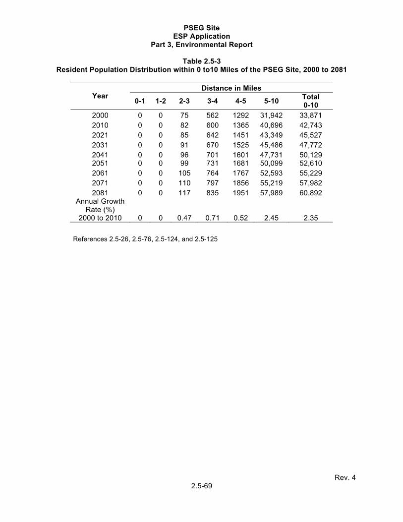
PSEG Site ESP Application
Part 3, Environmental Report
Rev. 4 2.5-69
Table 2.5-3 Resident Population Distribution within 0 to10 Miles of the PSEG Site, 2000 to 2081
Year Distance in Miles
0-1 1-2 2-3 3-4 4-5 5-10 Total 0-10
2000 0 0 75 562 1292 31,942 33,871 2010 0 0 82 600 1365 40,696 42,743 2021 0 0 85 642 1451 43,349 45,527 2031 0 0 91 670 1525 45,486 47,772 2041 0 0 96 701 1601 47,731 50,129 2051 0 0 99 731 1681 50,099 52,610 2061 0 0 105 764 1767 52,593 55,229 2071 0 0 110 797 1856 55,219 57,982 2081 0 0 117 835 1951 57,989 60,892
Annual Growth Rate (%)
2000 to 2010 0 0 0.47 0.71 0.52 2.45 2.35
References 2.5-26, 2.5-76, 2.5-124, and 2.5-125

PSEG Site ESP Application
Part 3, Environmental Report
Rev. 4 2.5-70
Table 2.5-4 Populations and Growth Rates of Municipalities within 10 Miles of the PSEG Site
Township/Municipality Population
2000 Population2007/2008a
Annual Growth Rate (%)
Population 2010
Salem County, New Jersey Lower Alloways Creek Township 1851 1883 0.25 1897 Quinton Township 2786 2838 0.26 2861 Elsinboro Township 1092 1054 -0.50 1038 Salem 5857 5678 -0.44 5603 Mannington Township 1559 1555 -0.04 1553 Pennsville Township 13,194 13,363 0.18 13,436 Total County 64,285 66,141 0.36 66,613
Cumberland County, New Jersey Stow Creek Township 1429 1528 0.96 1573 Greenwich Township 847 886 0.65 903 Total County 146,438 156,830 0.86 159,541
New Castle County, Delaware Odessa 286 334 2.24 357 Townsend 346 378 1.27 393 Middletown 6161 11,153 8.85 14,383 Delaware City 1453 1516 0.61 1544 Total County 500,265 529,641 0.72 537,251
References 2.5-122 and 2.5-125
a) 2008 estimates apply to counties, 2007 estimates apply to all others.

PSEG Site ESP Application
Part 3, Environmental Report
Rev. 4 2.5-71
Table 2.5-5 Transient Population Distribution within 10 Miles of the PSEG Site, 2008 to 2081
Year
Distance in Miles
0-1 1-2 2-3 3-4 4-5 5-10 Total 0-10
2008 0 0 0 163 97 11,825 12,085 2010 0 0 0 166 98 12,285 12,549 2021 0 0 0 176 105 13,097 13,378 2031 0 0 0 183 109 13,765 14,057 2041 0 0 0 191 116 14,470 14,777 2051 0 0 0 199 122 15,212 15,533 2061 0 0 0 206 129 15,997 16,332 2071 0 0 0 215 136 16,824 17,175 2081 0 0 0 224 143 17,696 18,063
References 2.5-27, 2.5-44, 2.5-47-- 2.5-51, and 2.5-76

PSEG Site ESP Application
Part 3, Environmental Report
Rev. 4 2.5-72
Table 2.5-6 Transient Population Estimates within 10 Miles of PSEG Site, 2008
Distance in Miles
Source of Transients
Employers Recreation Lodging Schools
and Daycare
Medical Care (Hospitals
and Assisted Living)
Totals
0-1 0 0 0 0 0 0
1-2 0 0 0 0 0 0
2-3 0 0 0 0 0 0
3-4 0 163 0 0 0 163
4-5 2 88 0 7 0 97
5-10 4144 2843 121 4114 603 11,825
0-10 4146 3094 121 4121 603 12,085
Percent 34 26 1 34 5 100
Delaware 2244 1899 80 3432 336 7991
Percent of Total 66
New Jersey 1902 1195 41 689 267 4094
Percent of Total 34
References 2.5-21, 2.5-44, and 2.5-47 to 2.5-51.

PSEG Site ESP Application
Part 3, Environmental Report
Rev. 4 2.5-73
Table 2.5-7 Resident Population Distribution within 10 to 50 Miles of the PSEG Site, 2000 to 2081(a)
Year
Population/Distance in Miles
10 – 20 20 – 30 30 – 40 40 – 50 Total
10 – 50 Total 0 – 50
2000 495,708 663,385 1,839,777 2,197,713 5,196,583 5,230,454
2010 535,164 737,825 1,907,693 2,237,530 5,418,212 5,460,955
2021 579,362 811,029 2,024,369 2,346,225 5,760,985 5,806,512
2031 612,502 875,214 2,134,825 2,434,175 6,056,716 6,104,488
2041 648,433 946,388 2,257,452 2,530,748 6,383,021 6,433,150
2051 687,502 1,025,479 2,393,789 2,636,891 6,743,661 6,796,271
2061 730,126 1,113,552 2,545,595 2,753,673 7,142,946 7,198,175
2071 776,789 1,211,819 2,714,864 2,882,300 7,585,772 7,643,754
2081 828,052 1,321,698 2,903,867 3,024,126 8,077,743 8,138,635
Annual Growth Rate
(%) 2000 to 2010 0.77 1.07 0.36 0.18 0.42 0.43 References 2.5-27, 2.5-60, 2.5-76, 2.5-89, 2.5-124, and 2.5-125 a) Population for 0-10 mile vicinity is shown in Table 2.5-3

PSEG Site ESP Application
Part 3, Environmental Report
Rev. 4 2.5-74
Table 2.5-8 (Sheet 1 of 4) Resident Population Distribution and Projections within 50 Miles of the PSEG Site
Year Sectors Population/Distance in Miles
0 – 1 1 –2 2 – 3 3 – 4 4 – 5 5 – 10 Total 0 – 10
10 – 20 20 – 30 30 – 40 40 – 50 Total
10 – 50 Total0 – 50
2000 N 0 0 0 0 110 224 334 139,009 121,179 157,479 154,146 571,813 572,147 2010 N 0 0 0 0 105 224 329 146,379 127,017 180,586 171,958 625,940 626,269 2021 N 0 0 0 0 112 240 352 155,730 134,747 210,005 194,320 694,802 695,154 2031 N 0 0 0 0 120 257 377 162,469 140,863 237,903 214,653 755,888 756,265 2041 N 0 0 0 0 129 275 404 169,510 147,356 269,731 237,612 824,209 824,613 2051 N 0 0 0 0 138 295 433 176,867 154,261 306,050 263,562 900,740 901,173 2061 N 0 0 0 0 148 316 464 184,555 161,618 347,503 292,921 986,597 987,061 2071 N 0 0 0 0 158 338 496 192,589 169,469 394,822 326,165 1,083,045 1,083,541 2081 N 0 0 0 0 170 362 532 200,986 177,866 448,847 363,839 1,191,538 1,192,070
2000 NNE 0 0 3 6 33 5611 5653 16,119 132,180 907,397 1,033,412
2,089,108 2,094,761 2010 NNE 0 0 3 5 31 5398 5437 17,013 135,920 883,240 1,003,853 2,040,026 2,045,463 2021 NNE 0 0 3 6 33 5775 5817 18,210 141,555 886,469 1,006,508 2,052,742 2,058,559 2031 NNE 0 0 4 6 36 6186 6232 19,519 147,943 896,061 1,012,808 2,076,331 2,082,563 2041 NNE 0 0 4 7 38 6627 6676 20,924 154,763 906,131 1,019,671 2,101,489 2,108,165 2051 NNE 0 0 4 7 41 7100 7152 22,430 162,055 916,696 1,027,119 2,128,300 2,135,452 2061 NNE 0 0 5 8 44 7606 7663 24,045 169,864 927,771 1,035,179 2,156,859 2,164,522 2071 NNE 0 0 5 8 47 8148 8208 25,777 178,240 939,374 1,043,880 2,187,271 2,195,479 2081 NNE 0 0 5 9 50 8729 8793 27,634 187,239 951,522 1,053,252 2,219,647 2,228,440 2000 NE 0 0 1 6 42 3240 3289 8542 68,340 423,003 492,289 992,174 995,463 2010 NE 0 0 1 5 42 3200 3248 9052 79,314 443,708 498,939 1,031,013 1,034,261 2021 NE 0 0 1 6 44 3423 3474 9707 88,435 473,816 525,180 1,097,138 1,100,612 2031 NE 0 0 2 6 48 3667 3723 10,425 98,741 503,842 550,506 1,163,514 1,167,237 2041 NE 0 0 2 7 51 3928 3988 11,198 110,249 536,375 577,796 1,235,618 1,239,606 2051 NE 0 0 2 7 55 4209 4273 12,029 123,099 571,658 607,203 1,313,989 1,318,262 2061 NE 0 0 2 8 59 4509 4578 12,924 137,449 609,960 638,891 1,399,224 1,403,802 2071 NE 0 0 2 8 63 4830 4903 13,887 153,473 651,580 673,037 1,491,977 1,496,880 2081 NE 0 0 2 9 67 5174 5252 14,923 171,366 696,849 709,835 1,592,973 1,598,225 2000 ENE 0 0 11 30 188 1130 1359 4420 34,671 87,605 42,859 169,555 170,914 2010 ENE 0 0 12 31 193 1160 1396 4681 39,356 94,959 45,462 184,458 185,854 2021 ENE 0 0 12 33 206 1240 1491 5006 43,441 103,127 49,543 201,117 202,608 2031 ENE 0 0 13 36 221 1329 1599 5353 48,004 111,616 53,473 218,446 220,045 2041 ENE 0 0 14 38 237 1424 1713 5724 53,066 120,923 57,732 237,445 239,158 2051 ENE 0 0 15 41 254 1525 1835 6120 58,682 131,133 62,349 258,284 260,119 2061 ENE 0 0 16 44 272 1634 1966 6545 64,915 142,343 67,355 281,158 283,124 2071 ENE 0 0 17 47 291 1750 2105 6999 71,834 154,660 72,783 306,276 308,381 2081 ENE 0 0 19 50 312 1875 2256 7485 79,517 168,204 78,672 333,878 336,134

PSEG Site ESP Application
Part 3, Environmental Report
Rev. 4 2.5-75
Table 2.5-8 (Sheet 2 of 4) Resident Population Distribution and Projections within 50 Miles of the PSEG Site
Year Sectors Population/Distance in Miles
0 – 1 1 – 2 2 – 3 3 – 4 4 – 5 5 – 10 Total 0 – 10
10 – 20 20 – 30 30 – 40 40 – 50 Total
10 – 50 Total0 – 50
2000 E 0 0 8 28 25 989 1050 24,456 68,481 21,954 41,989 156,880 157,930 2010 E 0 0 9 29 26 1020 1084 26,614 74,640 23,952 45,739 170,945 172,029 2021 E 0 0 9 31 28 1091 1159 28,407 79,806 26,125 50,365 184,703 185,862 2031 E 0 0 10 33 30 1166 1239 29,724 83,782 28,230 55,176 196,912 198,151 2041 E 0 0 11 36 32 1247 1326 31,103 87,973 30,520 60,446 210,042 211,368 2051 E 0 0 11 38 34 1333 1416 32,546 92,392 33,010 66,219 224,167 225,583 2061 E 0 0 12 41 36 1426 1515 34,056 97,054 35,721 72,543 239,374 240,889 2071 E 0 0 13 44 39 1525 1621 35,637 101,974 38,671 79,472 255,754 257,375 2081 E 0 0 14 47 42 1631 1734 37,292 107,168 41,884 87,062 273,406 275,140 2000 ESE 0 0 0 0 3 350 353 18,638 22,893 9952 22,939 74,422 74,775 2010 ESE 0 0 0 0 3 380 383 20,279 24,928 10,673 21,323 77,203 77,586 2021 ESE 0 0 0 0 3 405 408 21,644 26,606 11,362 22,000 81,612 82,020 2031 ESE 0 0 0 0 3 425 428 22,636 27,825 11,887 22,947 85,295 85,723 2041 ESE 0 0 0 0 3 446 449 23,674 29,100 12,437 23,939 89,150 89,599 2051 ESE 0 0 0 0 3 467 470 24,759 30,434 13,012 24,978 93,183 93,653 2061 ESE 0 0 0 0 4 490 494 25,893 31,829 13,615 26,067 97,404 97,898 2071 ESE 0 0 0 0 4 514 518 27,080 33,288 14,247 27,210 101,825 102,343 2081 ESE 0 0 0 0 4 539 543 28,321 34,813 14,908 28,408 106,450 106,993 2000 SE 0 0 0 0 0 6 6 90 588 37 39,744 40,459 40,465 2010 SE 0 0 0 0 0 6 6 97 641 40 36,596 37,374 37,380 2021 SE 0 0 0 0 0 6 6 104 684 43 37,592 38,423 38,429 2031 SE 0 0 0 0 0 7 7 108 715 45 39,073 39,941 39,948 2041 SE 0 0 0 0 0 7 7 113 748 47 40,611 41,519 41,526 2051 SE 0 0 0 0 0 7 7 118 782 49 42,211 43,160 43,167 2061 SE 0 0 0 0 0 8 8 124 818 51 43,873 44,866 44,874 2071 SE 0 0 0 0 0 8 8 130 856 53 45,601 46,640 46,648 2081 SE 0 0 0 0 0 9 9 135 895 56 47,396 48,482 48,491 2000 SSE 0 0 0 0 0 4 4 119 1200 1027 5588 7934 7938 2010 SSE 0 0 0 0 0 6 6 152 1539 1304 6981 9976 9982 2021 SSE 0 0 0 0 0 6 6 170 1726 1510 8528 11,934 11,940 2031 SSE 0 0 0 0 0 7 7 182 1847 1659 9750 13,438 13,445 2041 SSE 0 0 0 0 0 7 7 195 1976 1824 11,148 15,143 15,150 2051 SSE 0 0 0 0 0 8 8 209 2115 2007 12,745 17,076 17,084 2061 SSE 0 0 0 0 0 8 8 224 2264 2211 14,572 19,271 19,279 2071 SSE 0 0 0 0 0 9 9 239 2422 2439 16,660 21,760 21,769 2081 SSE 0 0 0 0 0 10 10 256 2592 2693 19,048 24,589 24,599

PSEG Site ESP Application
Part 3, Environmental Report
Rev. 4 2.5-76
Table 2.5-8 (Sheet 3 of 4) Resident Population Distribution and Projections within 50 Miles of the PSEG Site
Year Sectors Population/Distance in Miles
0 – 1 1 – 2 2 – 3 3 – 4 4 – 5 5 – 10 Total 0 – 10
10 – 20 20 – 30 30 – 40 40 – 50 Total
10 – 50 Total0 – 50
2000 S 0 0 0 0 3 111 114 10,744 62,964 26,379 16,824 116,911 117,025 2010 S 0 0 0 0 4 128 132 13,777 80,752 33,679 21,093 149,301 149,433 2021 S 0 0 0 0 4 139 143 15,453 90,578 38,350 25,476 169,857 170,000 2031 S 0 0 0 0 4 147 151 16,537 96,933 41,554 28,890 183,914 184,065 2041 S 0 0 0 0 4 154 158 17,697 103,733 45,056 32,777 199,263 199,421 2051 S 0 0 0 0 4 163 167 18,938 111,011 48,887 37,202 216,038 216,205 2061 S 0 0 0 0 5 171 176 20,266 118,800 53,084 42,243 234,393 234,569 2071 S 0 0 0 0 5 180 185 21,688 127,135 57,684 47,985 254,492 254,677 2081 S 0 0 0 0 5 190 195 23,209 136,055 62,733 54,529 276,526 276,721 2000 SSW 0 0 0 4 6 566 576 16,445 11,543 9480 14,309 51,777 52,353 2010 SSW 0 0 0 4 7 612 623 20,410 14,540 11,162 16,338 62,450 63,073 2021 SSW 0 0 0 4 7 651 662 22,708 16,471 13,139 19,344 71,662 72,324 2031 SSW 0 0 0 5 7 677 689 24,202 17,802 14,720 21,791 78,515 79,204 2041 SSW 0 0 0 5 8 705 718 25,798 19,249 16,501 24,564 86,112 86,830 2051 SSW 0 0 0 5 8 734 747 27,501 20,825 18,511 27,709 94,546 95,293 2061 SSW 0 0 0 5 8 764 777 29,319 22,542 20,779 31,274 103,914 104,691 2071 SSW 0 0 0 5 9 795 809 31,260 24,413 23,340 35,319 114,332 115,141 2081 SSW 0 0 0 6 9 828 843 33,333 26,456 26,232 39,908 125,929 126,772 2000 SW 0 0 1 6 7 1635 1649 3785 5345 5739 9719 24,588 26,237 2010 SW 0 0 1 6 8 1772 1787 4269 6256 6815 11,477 28,817 30,604 2021 SW 0 0 1 7 8 1885 1901 4645 7170 7856 13,174 32,845 34,746 2031 SW 0 0 1 7 9 1962 1979 4890 7878 8687 14,513 35,968 37,947 2041 SW 0 0 1 7 9 2042 2059 5149 8661 9607 15,995 39,412 41,471 2051 SW 0 0 1 8 9 2126 2144 5423 9525 10,627 17,634 43,209 45,353 2061 SW 0 0 2 8 10 2213 2233 5712 10,481 11,757 19,447 47,397 49,630 2071 SW 0 0 2 8 10 2303 2323 6018 11,536 13,010 21,455 52,019 54,342 2081 SW 0 0 2 9 11 2398 2420 6341 12,703 14,398 23,676 57,118 59,538 2000 WSW 0 0 1 15 142 2979 3137 3297 3450 10,912 26,875 44,534 47,671 2010 WSW 0 0 2 16 154 4262 4434 3687 3722 11,737 28,284 47,430 51,864 2021 WSW 0 0 2 17 163 4532 4714 4303 4170 13,003 29,950 51,426 56,140 2031 WSW 0 0 2 18 170 4718 4908 4782 4454 13,760 30,266 53,262 58,170 2041 WSW 0 0 2 19 177 4911 5109 5335 4764 14,564 30,592 55,255 60,364 2051 WSW 0 0 2 19 184 5112 5317 5975 5104 15,422 30,928 57,429 62,746 2061 WSW 0 0 2 20 192 5321 5535 6718 5479 16,335 31,275 59,807 65,342 2071 WSW 0 0 2 21 200 5539 5762 7582 5893 17,309 31,632 62,416 68,178 2081 WSW 0 0 2 22 208 5766 5998 8588 6352 18,349 32,002 65,291 71,289

PSEG Site ESP Application
Part 3, Environmental Report
Rev. 4 2.5-77
Table 2.5-8 (Sheet 4 of 4) Resident Population Distribution and Projections within 50 Miles of the PSEG Site
Year Sectors Population/Distance in Miles
0 – 1 1 – 2 2 – 3 3 – 4 4 – 5 5 – 10 Total 0 – 10
10 – 20 20 – 30 30 – 40 40 – 50 Total
10 – 50 Total0 – 50
2000 W 0 0 2 124 298 7366 7790 4983 5245 50,087 180,185 240,500 248,290 2010 W 0 0 2 134 322 14,199 14,657 6170 6108 56,270 198,557 267,105 281,762 2021 W 0 0 2 143 343 15,099 15,587 7274 7366 62,969 218,504 296,113 311,700 2031 W 0 0 2 148 357 15,718 16,225 8181 8219 64,348 222,304 303,052 319,277 2041 W 0 0 2 154 371 16,361 16,888 9237 9218 65,758 226,183 310,396 327,284 2051 W 0 0 2 161 386 17,031 17,580 10,471 10,391 67,198 230,141 318,201 335,781 2061 W 0 0 2 167 402 17,729 18,300 11,913 11,770 68,669 234,180 326,532 344,832 2071 W 0 0 2 174 419 18,455 19,050 13,602 13,391 70,173 238,303 335,469 354,519 2081 W 0 0 3 181 436 19,211 19,831 15,582 15,301 71,710 242,510 345,103 364,934 2000 WNW 0 0 48 150 255 3614 4067 22,539 25,101 29,728 23,971 101,339 105,406 2010 WNW 0 0 52 162 276 3906 4396 26,208 30,162 34,621 26,919 117,910 122,306 2021 WNW 0 0 55 173 293 4154 4675 32,151 38,578 41,817 29,726 142,272 146,947 2031 WNW 0 0 57 180 305 4324 4866 37,126 45,710 47,031 30,866 160,733 165,599 2041 WNW 0 0 60 187 318 4501 5066 42,982 54,163 53,142 32,063 182,350 187,416 2051 WNW 0 0 62 195 331 4685 5273 49,881 64,181 60,313 33,321 207,696 212,969 2061 WNW 0 0 64 203 344 4877 5488 58,012 76,052 68,738 34,644 237,446 242,934 2071 WNW 0 0 67 211 358 5077 5713 67,604 90,120 78,647 36,035 272,406 278,119 2081 WNW 0 0 70 220 373 5284 5947 78,925 106,793 90,311 37,500 313,529 319,476 2000 NW 0 0 0 112 155 2429 2696 97,184 27,214 27,081 42,640 194,119 196,815 2010 NW 0 0 0 121 167 2625 2913 104,022 31,899 31,100 46,300 213,321 216,234 2021 NW 0 0 0 129 178 2791 3098 113,104 38,686 35,933 49,289 237,012 240,110 2031 NW 0 0 0 134 185 2906 3225 119,859 44,703 40,473 51,956 256,991 260,216 2041 NW 0 0 0 140 193 3025 3358 127,285 51,704 45,634 54,781 279,404 282,762 2051 NW 0 0 0 145 201 3148 3494 135,481 59,853 51,501 57,775 304,610 308,104 2061 NW 0 0 0 151 209 3277 3637 144,565 69,343 58,177 60,949 333,034 336,671 2071 NW 0 0 0 157 218 3412 3787 154,675 80,401 65,775 64,317 365,168 368,955 2081 NW 0 0 0 164 227 3551 3942 165,975 93,291 74,425 67,892 401,583 405,525 2000 NNW 0 0 0 81 25 1688 1794 125,338 72,991 71,917 50,224 320,470 322,264 2010 NNW 0 0 0 87 27 1798 1912 132,354 81,031 83,847 57,711 354,943 356,855 2021 NNW 0 0 0 93 29 1912 2034 140,746 91,010 98,845 66,726 397,327 399,361 2031 NNW 0 0 0 97 30 1990 2117 146,509 99,795 113,009 75,203 434,516 436,633 2041 NNW 0 0 0 101 31 2071 2203 152,509 109,665 129,202 84,838 476,214 478,417 2051 NNW 0 0 0 105 33 2156 2294 158,754 120,769 147,715 95,795 523,033 525,327 2061 NNW 0 0 0 109 34 2244 2387 165,255 133,274 168,881 108,260 575,670 578,057 2071 NNW 0 0 0 114 35 2336 2485 172,022 147,374 193,080 122,446 634,922 637,407 2081 NNW 0 0 0 118 37 2432 2587 179,067 163,291 220,746 138,597 701,701 704,288
References 2.5-26, 2.5-60, 2.5-76, 2.5-89, 2.5-124, and 2.5-125
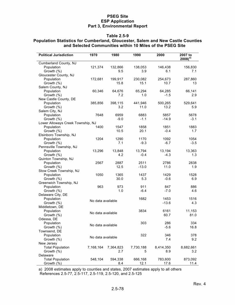
PSEG Site ESP Application
Part 3, Environmental Report
Rev. 4 2.5-78
Table 2.5-9 Population Statistics for Cumberland, Gloucester, Salem and New Castle Counties
and Selected Communities within 10 Miles of the PSEG Site
Political Jurisdiction 1970 1980 1990 2000 2007 to2008(a)
Cumberland County, NJ Population 121,374 132,866 138,053 146,438 156,830 Growth (%) 9.5 3.9 6.1 7.1
Gloucester County, NJ Population 172,681 199,917 230,082 254,673 287,860 Growth (%) 15.8 15.1 10.7 13
Salem County, NJ Population 60,346 64,676 65,294 64,285 66,141 Growth (%) 7.2 1.0 -1.5 2.9
New Castle County, DE Population 385,856 398,115 441,946 500,265 529,641 Growth (%) 3.2 11.0 13.2 5.9
Salem City, NJ Population 7648 6959 6883 5857 5678 Growth (%) -9.0 -1.1 -14.9 -3.1
Lower Alloways Creek Township, NJ Population 1400 1547 1858 1851 1883 Growth (%) 10.5 20.1 -0.4 1.7
Elsinboro Township, NJ Population 1204 1290 1170 1092 1054 Growth (%) 7.1 -9.3 -6.7 -3.5
Pennsville Township, NJ Population 13,296 13,848 13,794 13,194 13,363 Growth (%) 4.2 -0.4 -4.3 1.3
Quinton Township, NJ Population 2567 2887 2511 2786 2838 Growth (%) 12.5 -13.0 11.0 1.9
Stow Creek Township, NJ Population 1050 1365 1437 1429 1528 Growth (%) 30.0 5.3 -0.6 6.9
Greenwich Township, NJ Population 963 973 911 847 886 Growth (%) 1.0 -6.4 -7.0 4.6
Delaware City, DE Population
No data available 1682 1453 1516
Growth (%) -13.6 4.3 Middletown, DE
Population No data available
3834 6161 11,153 Growth (%) 60.7 81.0
Odessa, DE Population
No data available 303 286 334
Growth (%) -5.6 16.8 Townsend, DE
Population No data available
322 346 378 Growth (%) 7.4 9.2
New Jersey Total Population 7,168,164 7,364,823 7,730,188 8,414,350 8,682,661 Growth (%) 2.7 5 8.9 3.2
Delaware Total Population 548,104 594,338 666,168 783,600 873,092 Growth (%) 8.4 12.1 17.6 11.4
a) 2008 estimates apply to counties and states, 2007 estimates apply to all others References 2.5-77, 2.5-117, 2.5-119, 2.5-120, and 2.5-125

PSEG Site ESP Application
Part 3, Environmental Report
Rev. 4 2.5-79
Table 2.5-10 (Sheet 1 of 3) Population Characteristics for Counties and Selected Communities within 10 Miles of the PSEG Site(a)
Population Characteristics
Census 2000 Demographic Profile 2005-2007 ACS 3-Year Estimates Cumberland
County Gloucester
County Salem
County New
Jersey United States
Cumberland County
Gloucester County
Salem County
New Jersey
United States
Gender Male (%) 51.0 48.4 48.3 48.5 49.1 51.5 48.7 48.8 48.9 49.2 Female (%) 49.0 51.6 51.7 51.5 50.9 48.5 51.3 51.2 51.1 50.8 Age Under 5 years (%) 6.3 6.6 6.1 6.7 6.8 7.2 6.0 5.9 6.5 6.9 18 years and over (%) 74.6 73.6 74.4 75.2 74.3 75.5 76.1 76.7 76.0 75.3 65 years and over (%) 13.0 11.7 14.5 13.2 12.4 12.4 11.5 13.9 13.0 12.5 Median Age 35.6 36.1 38.0 36.7 35.3 35.9 37.3 39.2 38.2 36.4 Race/Ethnicity (%) White 65.9 87.1 81.2 72.6 75.1 66.9 84.8 80.2 69.7 74.1 Black 20.2 9.1 14.8 13.6 12.3 20.8 9.6 15.5 13.6 12.4 Asian 1.0 1.5 0.6 5.7 3.6 1.1 2.2 0.5 7.3 4.3 Hispanic 19.0 2.6 3.9 13.3 12.5 22.7 3.5 4.9 15.6 14.7 Foreign Born 6.2 3.4 2.5 17.5 11.1 8.3 4.3 2.8 19.7 12.5 Home language not English 20.4 6.5 6.3 25.5 17.9 22.0 7.1 7.2 27.5 19.5
Per capita income $17,376 $22,708 $20,874 $27,006 $21,587 $21,060 $29,627 $26,581 $33,219 $26,178 Families below poverty (%) 11.3 4.3 7.2 6.3 9.2 13.4 5.4 6.3 6.5 9.8
Individuals below poverty (%) 15.0 6.2 9.5 8.5 12.4 15.1 7.3 9.9 8.7 13.3
Average household size 2.7 2.8 2.6 2.7 2.6 2.9 2.8 2.6 2.7 2.6 Average family size 3.2 3.2 3.1 3.2 3.1 3.5 3.3 3.1 3.3 3.2
High school graduates (%) 68.5 84.3 79.4 82.1 80.4 73.1 88.3 85.7 86.3 84.0 College graduates (%) 11.7 22.0 15.2 29.8 24.4 12.7 25.6 18.0 33.7 27.0
Owner-occupied housing (%) 67.9 79.9 73.0 65.6 66.2 68.4 81.5 75.1 67.4 67.3
Median value owner-occupied $91,200 $120,100 $105,200 $170,800 $119,600 $156,500 $220,400 $173,600 $358,400 $181,800
Housing vacant (%) 7.0 4.6 7.1 7.4 9.0 8.4 5.4 8.2 9.5 11.6

PSEG Site ESP Application
Part 3, Environmental Report
Rev. 4 2.5-80
Table 2.5-10 (Sheet 2 of 3) Population Characteristics for Counties and Selected Communities within 10 Miles of the PSEG Site(a)
Population Characteristics
Census 2000 Demographic Profile
Salem City Elsinboro Township
Lower Alloways Township
Quinton Township
Pennsville Township
Stow Creek Township
Greenwich Township
Gender Male (%) 44.6 47.4 48.3 49.9 48.0 49.2 49.6 Female (%) 55.4 52.6 51.7 50.1 52.0 50.8 50.4 Age Under 5 years (%) 8.8 4.8 6.5 5.8 5.7 5.2 5.5 18 years and over (%) 69.0 78.8 75.6 76.4 76.8 76.5 78.0 65 years and over (%) 14.0 19.8 13.9 15.8 15.5 14.5 14.9 Median Age 33.5 43.6 39.5 39.0 39.3 40.7 43.4 Race/Ethnicity (%) White 37.5 95.1 96.4 82.1 96.7 93.4 90.0 Black 56.8 3.6 2.2 14.5 1.0 3.5 5.1 Asian 0.2 0.0 0.6 0.3 1.0 0.2 0.2 Hispanic 4.9 0.6 0.5 1.5 1.6 1.7 1.5 Foreign Born 0.8 0.6 0.8 1.8 3.2 2.0 0.5 Home language not English 6.3 1.6 2.6 4.9 5.8 3.9 1.6 Per capita income $13,559 $25,415 $21,962 $18,921 $22,717 $20,925 $22,233 Families below poverty (%) 24.7 2.1 4.2 7.8 3.1 5.7 6.1 Individuals below poverty (%) 26.6 1.7 7.3 9.3 4.9 6.7 8.0 Average household size 2.4 2.3 2.7 2.6 2.5 2.7 2.6 Average family size 3.1 2.8 3.0 3.0 3.0 3.0 3.1 High school graduates (%) 67.8 83.9 82.4 72.1 82.0 83.1 86.3 College graduates (%) 7.9 16.5 11.7 10.3 13.6 18.9 22.0 Owner-occupied housing (%) 41.0 86.1 81.1 84.0 75.4 87.9 86.2 Median value owner-occupied $74,300 $110,100 $118,000 $101,300 $103,700 $114,400 $112,000 Housing vacant (%) 16.8 11.7 5.1 5.2 5.4 4.3 9.7
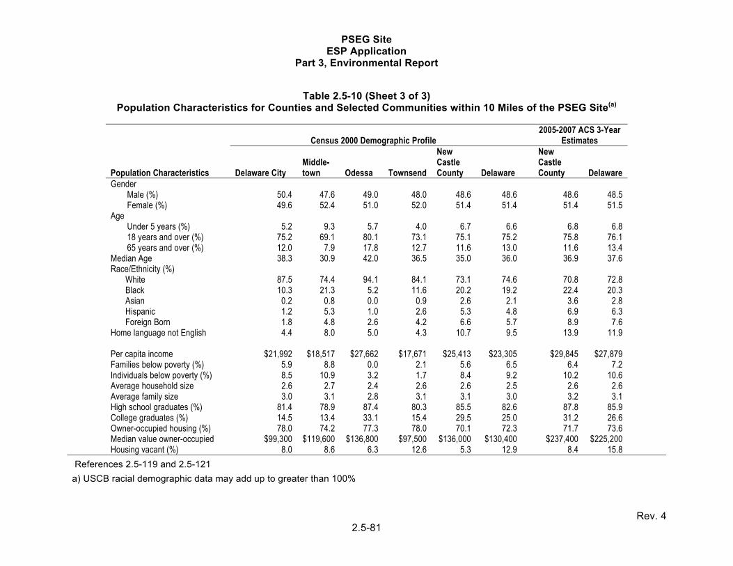
PSEG Site ESP Application
Part 3, Environmental Report
Rev. 4 2.5-81
Table 2.5-10 (Sheet 3 of 3)
Population Characteristics for Counties and Selected Communities within 10 Miles of the PSEG Site(a)
Population Characteristics
Census 2000 Demographic Profile 2005-2007 ACS 3-Year
Estimates
Delaware City Middle-town Odessa Townsend
New Castle County Delaware
New Castle County Delaware
Gender Male (%) 50.4 47.6 49.0 48.0 48.6 48.6 48.6 48.5 Female (%) 49.6 52.4 51.0 52.0 51.4 51.4 51.4 51.5 Age Under 5 years (%) 5.2 9.3 5.7 4.0 6.7 6.6 6.8 6.8 18 years and over (%) 75.2 69.1 80.1 73.1 75.1 75.2 75.8 76.1 65 years and over (%) 12.0 7.9 17.8 12.7 11.6 13.0 11.6 13.4 Median Age 38.3 30.9 42.0 36.5 35.0 36.0 36.9 37.6 Race/Ethnicity (%) White 87.5 74.4 94.1 84.1 73.1 74.6 70.8 72.8 Black 10.3 21.3 5.2 11.6 20.2 19.2 22.4 20.3 Asian 0.2 0.8 0.0 0.9 2.6 2.1 3.6 2.8 Hispanic 1.2 5.3 1.0 2.6 5.3 4.8 6.9 6.3 Foreign Born 1.8 4.8 2.6 4.2 6.6 5.7 8.9 7.6 Home language not English 4.4 8.0 5.0 4.3 10.7 9.5 13.9 11.9 Per capita income $21,992 $18,517 $27,662 $17,671 $25,413 $23,305 $29,845 $27,879 Families below poverty (%) 5.9 8.8 0.0 2.1 5.6 6.5 6.4 7.2 Individuals below poverty (%) 8.5 10.9 3.2 1.7 8.4 9.2 10.2 10.6 Average household size 2.6 2.7 2.4 2.6 2.6 2.5 2.6 2.6 Average family size 3.0 3.1 2.8 3.1 3.1 3.0 3.2 3.1 High school graduates (%) 81.4 78.9 87.4 80.3 85.5 82.6 87.8 85.9 College graduates (%) 14.5 13.4 33.1 15.4 29.5 25.0 31.2 26.6 Owner-occupied housing (%) 78.0 74.2 77.3 78.0 70.1 72.3 71.7 73.6 Median value owner-occupied $99,300 $119,600 $136,800 $97,500 $136,000 $130,400 $237,400 $225,200 Housing vacant (%) 8.0 8.6 6.3 12.6 5.3 12.9 8.4 15.8
References 2.5-119 and 2.5-121
a) USCB racial demographic data may add up to greater than 100%

PSEG Site ESP Application
Part 3, Environmental Report
Rev. 4 2.5-82
Table 2.5-11 Schools and Daycare Facilities within 10 Miles of the PSEG Site
Schools and Daycare Centers Sector Distance in
Miles Delaware
ABC1 Child Care Learning W 9.6 AdvoServe School NW 9.4 Alfred Waters Middle School WNW 8.1 Appoquinimink Early Childhood Center WSW 9.6 Bethesda Child Development Center W 9.4 Brick Mill Elementary School W 7.9 Bright Beginnings Preschool WNW 8.0 Cedar Lane Elementary School WNW 8.0 Cedar Lane Early Childhood Center WNW 8.0 Everett Meredith Middle School WSW 9.6 Green Acres Preschool W 6.5 Gunning Bedford Middle School NW 7.8 Groves Adult High School WSW 9.6 Kathleen H. Wilbur (Wrangle Hill) Elementary School NW 10.0 Louis L. Redding Middle School W 9.1 Middletown High School W 8.3 Silver Lake Elementary School W 9.3 St. Andrews School WSW 8.5 St. Anne's Episcopal School WSW 8.9 St. George's Technical High School WNW 7.7 Southern Elementary School NW 7.7 Townsend Elementary School WSW 9.6 Townsend Early Childhood Center SW 9.5 Van Hook Walsh School, Inc. NW 5.8
New Jersey The ARC of Salem County NNE 9.0 Children’s Space Child Care NNE 7.4 Community Center NNE 7.7 Community Center NE 7.7 Elsinboro Township Elementary School NNE 5.4 John Fenwick Elementary School NNE 7.4 Lower Alloways Creek Elementary School E 7.0 Noah’s Ark NE 7.6 Quinton Elementary School NE 8.4 St. John’s Pentecostal Outreach Day Care Center NNE 7.8 Salem City High School NNE 6.8 Salem City Middle School NNE 7.6 Salvation Army Services Center NNE 7.8 Silver Lake Elementary School W 9.3 Sugar & Spice Preschool Day Care Center ENE 4.8 Reference 2.5-44

PSEG Site ESP Application
Part 3, Environmental Report
Rev. 4 2.5-83
Table 2.5-12 Employment Locations within 10 Miles of the PSEG Site
Employment Locations Sector Distance in
Miles Delaware
Air Liquide American LP NNW 8.0 Blackbird Landing Group Home(a) SW 8.4 Broadmeadow Healthcare(a) WSW 9.7 Cornerstone Residential(a) NNW 7.2 DelStar Technologies W 9.8 Formosa Plastics NW 9.6 Gateway Foundation (Cottage 2) (a) NNW 7.2 Governor Bacon Health Center(a) NNW 7.2 Johnson Controls, Inc W 9.7 Letica Corporation WNW 9.8 MacDermid Autotype, Inc. WSW 9.9 Middletown Residential Treatment Center(a) W 8.6 Quaker City Motor Parts/NAPA Dist. Center W 9.7 Silver Lake Day Treatment Center(a) W 8.6 Valero (Delaware City Refinery)(b) NNW 8.9
New Jersey
Anchor Hocking Glass NNE 8.0 Cooper Interconnect NNE 7.6 Homecare & Hospicecare of South Jersey(a) NNE 7.8 Lindsay House(a) NNE 9.5 Lower Alloways Creek Twp: Leisure Arms
Complex(a) ENE 5.9
Mannington Mills, Inc NNE 8.7 Memorial Hospital of Salem County(a) NNE 8.0 Midtown Rest Haven(a) NNE 7.8 National Freight, Inc. NNE 8.3 Office of Salem County NNE 7.9 PSEG (EERC) NNE 6.9 Salem County Mannington Center NNE 9.1 The ARC of Salem County NNE 9.0
References 2.5-44, 2.5-47 thru 2.5-51 a) Medical care facilities b) Industrial employer closed in 2009. Facilities remain in place and are available for reuse. Other employment locations include schools listed in Table 2.5-11.

PSEG Site ESP Application
Part 3, Environmental Report
Rev. 4 2.5-84
Table 2.5-13 Other Special Facilities within 10 Miles of the PSEG Site
Special Facilities State Sector Distance in
Miles Parks and Recreation
Aquatic Resource Education Center DE S 9.9 Augustine Beach Boat Ramp DE NW 3.1 Augustine Wildlife Area DE NNW 3.6 Cedar Swamp: Collins Beach DE S 6.0 Cedar Swamp: The Rock Tract DE SW 4.1 Chesapeake & Delaware Canal DE NW 6.7 Delaware City Marina DE NNW 7.4 Fort Delaware State Park DE NNW 7.9 Fort DuPont State Park DE NNW 7.2 Frog Hollow Golf Club DE W 9.1 Grass Dale Center DE NNW 6.6 Port Penn Interpretive Center DE NW 3.7 Sliver Lake Park DE W 9.2 Vandergrift Golf Club DE WNW 5.8
Abbot's Farm NJ NE 4.4 Barber's Basin, Inc. NJ NNE 7.5 Country Club of Salem NJ NNE 6.1 Fort Mott State Park NJ N 9.0 Hancock House NJ ENE 4.9 Mad Horse Creek WMA NJ ESE 7.1 Meadow View Acres Campground NJ E 7.8 Penn-Salem Marina NJ NNE 8.0 Salem Public Ramp (PSEG) NJ NNE 7.3 Salem Boat Club NJ NNE 8.2 Stow Creek State Park NJ ESE 7.3 Supawna Meadows National Wildlife Refuge NJ N 9.5 Wild Oaks Country Club NJ ENE 7.4
Lodging
Mallard Lodge DE S 9.9 Parkway Motel DE WNW 6.2 Pleasant Hill Motel DE WSW 6.9 Salem Motor Lodge NJ NNE 7.8
Reference 2.5-44
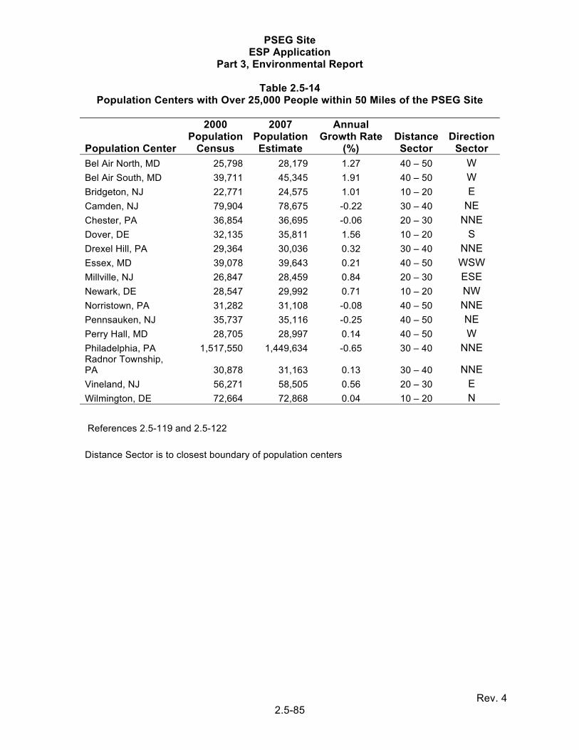
PSEG Site ESP Application
Part 3, Environmental Report
Rev. 4 2.5-85
Table 2.5-14 Population Centers with Over 25,000 People within 50 Miles of the PSEG Site
Population Center
2000 Population
Census
2007 Population Estimate
Annual Growth Rate
(%) Distance Sector
Direction Sector
Bel Air North, MD 25,798 28,179 1.27 40 – 50 W Bel Air South, MD 39,711 45,345 1.91 40 – 50 W Bridgeton, NJ 22,771 24,575 1.01 10 – 20 E Camden, NJ 79,904 78,675 -0.22 30 – 40 NE Chester, PA 36,854 36,695 -0.06 20 – 30 NNE Dover, DE 32,135 35,811 1.56 10 – 20 S Drexel Hill, PA 29,364 30,036 0.32 30 – 40 NNE Essex, MD 39,078 39,643 0.21 40 – 50 WSW Millville, NJ 26,847 28,459 0.84 20 – 30 ESE Newark, DE 28,547 29,992 0.71 10 – 20 NW Norristown, PA 31,282 31,108 -0.08 40 – 50 NNE Pennsauken, NJ 35,737 35,116 -0.25 40 – 50 NE Perry Hall, MD 28,705 28,997 0.14 40 – 50 W Philadelphia, PA 1,517,550 1,449,634 -0.65 30 – 40 NNE Radnor Township, PA 30,878 31,163 0.13 30 – 40 NNE Vineland, NJ 56,271 58,505 0.56 20 – 30 E Wilmington, DE 72,664 72,868 0.04 10 – 20 N
References 2.5-119 and 2.5-122
Distance Sector is to closest boundary of population centers

PSEG Site ESP Application
Part 3, Environmental Report
Rev. 4 2.5-86
Table 2.5-15 Description of Sparseness and Proximity Demographic Categories
Demographic Categories Based on Sparseness Category Description Most sparse 1. Less than 40 persons per sq. mi. and no community with
25,000 or more persons within 20 mi. 2. 40 to 60 persons per sq. mi. and no community with
25,000 or more persons within 20 mi. 3. 60 to 120 persons per sq. mi. or less than 60 persons per
sq. mi. with at least one community with 25,000 or more persons within 20 mi.
Least sparse 4. Greater than or equal to 120 persons per sq. mi. within 20 mi.
Demographic Categories Based on Proximity Category Description Not in close proximity 1. No city with 100,000 or more persons and less than
50 persons per sq. mi. within 50 mi. 2. No city with 100,000 or more persons and between 50
and 190 persons per sq. mi. within 50 mi. 3. One or more cities with 100,000 or more persons and
less than 190 persons per sq. mi. within 50 mi. In close proximity 4. Greater than or equal to 190 persons per sq. mi. within 50
mi.
NUREG-1437

PSEG Site ESP Application
Part 3, Environmental Report
Rev. 4 2.5-87
Table 2.5-16
Generic Environmental Impact Statement Sparseness and Proximity Matrix
Proximity Value 1 2 3 4
Sp
ars
en
ess
V
alu
e 1 1.1 1.2 1.3 1.4
2 2.1 2.2 2.3 2.4
3 3.1 3.3 3.3 3.4
4 4.1 4.2 4.3 4.4 Low Population Area Medium Population Area High Population Area NUREG-1437

PSEG Site ESP Application
Part 3, Environmental Report
Rev. 4 2.5-88
Table 2.5-17 Operation-Related Payroll for HCGS and SGS (2005 to 2008) for States and
Counties within 50 Miles of the PSEG Site
State County
Number of Employees Total Payroll Range Average Percent 2005 to 2008 Percent
Delaware Kent 1 – 2 2 0.1% $801,650 0.1%New Castle 254 – 269 261 17.4% $112,544,189 18.3%Subtotal 256 – 271 263 17.5% $113,345,839 18.5%
Maryland Cecil 27 – 33 29 1.9% $12,552,333 2.0%Harford 3 3 0.2% $1,481,635 0.2%Subtotal 30 – 36 32 2.1% $14,033,968 2.2%
New Jersey Atlantic 3 – 5 4 0.3% $1,729,482 0.3%Burlington 33 – 38 36 2.4% $15,133,933 2.5%Camden 56 – 68 64 4.2% $25,820,401 4.2%Cape May 5 – 7 6 0.4% $2,682,541 0.4%Cumberland 148 – 161 155 10.3% $60,774,838 9.9%Gloucester 210 – 230 220 14.6% $92,672,170 15.1%Salem 586 – 645 614 40.8% $234,000,031 38.1%Subtotal 1072 – 1135 1099 73.0% $432,813,395 70.5%
Pennsylvania Berks 3-4 4 0.2% $1,677,594 0.3%Bucks 0 – 1 0 0.0% $7,606 >0.1%Chester 37 – 56 45 3.0% $25,929,807 4.2%Delaware 29 – 39 34 2.3% $14,528,833 2.4%Lancaster 4 – 6 5 0.3% $2,701,025 0.4%Montgomery 5 – 9 7 0.4% $3,371,928 0.5%Philadelphia 1 – 2 1 0.1% $139,441 >0.1%Subtotal 79 – 116 96 6.3% $48,356,234 7.9%
Total 18 Counties $608,549,436 99.1%Total Four Counties(a) 1211 – 1300 1250 83.1% $499,991,227 81.4%Total Delaware 256 – 271 263 17.5% $113,345,839 18.5%Total Maryland 30 – 38 32 2.1% $14,296,461 2.3%Total New Jersey 1072 – 1140 1101 73.2% $433,607,381 70.6%Total Pennsylvania 84 – 122 101 6.7% $50,637,062 8.2%Counties Outside
50-Mile Area 12 – 19 16 1.1% $5,703,216 0.9%Other States 5 – 12 7 0.5% $2,365,910 0.4%Total All States 1453 – 1574 1504 100% $614,252,652 100%
a) New Castle (DE), Cumberland (NJ), Gloucester (NJ), and Salem (NJ)

PSEG Site ESP Application
Part 3, Environmental Report
Rev. 4 2.5-89
Table 2.5-18 (Sheet 1 of 2) Top Employers for Counties within 50 Miles of the PSEG Site
Location County Industry Employees
Three Delaware Counties State of Delaware Government(a) All Government 17,346 State Schools and Universities(a) All Education 16,655 Christiana Care Health System(b) New Castle Healthcare 10,790 E.I. Dupont(b) New Castle Manufacturing 9484 Dover Air Force Base(b) Kent Government 8595 Bank of America(b) New Castle Finance 8000 JP Morgan Chase & Co.(b) New Castle Finance 6500 AstraZeneca(b) New Castle Manufacturing 4600 Wal-Mart, Inc.(a) New Castle Retail 3932 Mountainaire Farms of DelMarVa(a) Sussex Agriculture 3513 Dover Downs, Inc.(a) Kent Entertainment 2929 Bayhealth Medical Center(a) Kent Healthcare 2915 Alfred. I. Dupont Institute(a) New Castle Healthcare 2745 Perdue Farms, Inc.(a) Sussex Agriculture 2672 Wilmington Trust(c) All Finance 2500 Total 103,176
Seven Maryland Counties Baltimore County Public Schools Baltimore Education 13,976 Aberdeen Proving Ground Harford Government 12,200 Social Security Administration Baltimore Government 9800 Baltimore County Government Baltimore Government 8568 Greater Baltimore Medical Center Baltimore Healthcare 3331 Centers for Medicare & Medicaid
Services—CMS Baltimore Government 2968
Erickson Retirement Communities Baltimore Healthcare 2809 Franklin Square Hospital Center Baltimore Healthcare 2800 W. L. Gore & Associates Cecil Manufacturing 2667 T. Rowe Price Associates, Inc. Baltimore Finance 2600 Reversal North America Inc. Baltimore Manufacturing 2530 University of Maryland Baltimore
County Baltimore Education 2490
St. Joseph Medical Center Baltimore Healthcare 2300 McCormick & Company, Inc. Baltimore Manufacturing 2267 CareFirst, Inc. Baltimore Healthcare 1962 Upper Chesapeake Health Medical
Services Harford Healthcare 1932
Lockheed Martin Baltimore Manufacturing 1800 Towson University Baltimore Education 1783 BD Diagnostic Systems Baltimore Manufacturing 1700 Solo Cup Company Baltimore Manufacturing 1700 Total 82,183
Seven New Jersey Counties Lockheed Martin Burlington Manufacturing 10,873 Borgata Hotel and Casino (2008 Atlantic Entertainment 6840 Virtua - West Jersey Health System Burlington and Camden Healthcare 7716 PHH Corp. Burlington Finance 5080 Bally's Park Place Atlantic Entertainment 4759 Trump Taj Mahal Atlantic Entertainment 4096

PSEG Site ESP Application
Part 3, Environmental Report
Rev. 4 2.5-90
Table 2.5-18 (Sheet 2 of 2) Top Employers for Counties within 50 Miles of the PSEG Site
Location County Industry Employees Cooper University Hospital Camden Healthcare 5284 Harrah's Atlantic Entertainment 4001 Caesar's Atlantic Entertainment 3645 Aztar Corporation Atlantic Entertainment 3517 Lourdes Health System Burlington and Camden Healthcare 3002 Federal Aviation Administration Atlantic Government 2950 Showboat Casino and Hotel Atlantic Entertainment 2710 Commerce Bank of Burlington Burlington Finance 2664 South Jersey Hospital System Cumberland Healthcare 2581 Resorts Casino Atlantic Entertainment 2422 Trump Plaza Atlantic Entertainment 2406 Kennedy Health System Camden Healthcare 2331 Hilton Hotel and Casino Atlantic Entertainment 2261 Underwood Memorial Hospital Gloucester Healthcare 2200 Total 81,338
Eight Pennsylvania Counties U.S. Government Philadelphia Government 52,000 Jefferson Health System Philadelphia Healthcare 23,000 School District of Philadelphia Philadelphia Education 26,000 City of Philadelphia Philadelphia Government 30,000 University of Pennsylvania Philadelphia Education 20,381 Catholic Archdiocese Philadelphia Education 15,400 University of Pennsylvania Health
Systems Philadelphia Healthcare
14,487 Comcast Corporation Philadelphia Information 12,795 Merck & Company, Inc. Montgomery Manufacturing 12,500 Catholic Health East Chester and Philadelphia Healthcare 11,834 Main Line Health Systems Montgomery Healthcare 9990 United Parcel Service Philadelphia Transportation 9919 Aramark Philadelphia Food Service 9450 Vanguard Group Chester Finance 9200 Children's Hospital of Philadelphia Philadelphia Healthcare 9150 Southeastern Pennsylvania
Transportation Authority Philadelphia Transportation
8800 Verizon Communications, Inc. Philadelphia Information 8800 WaWa, Inc. Delaware Retail 8170 Independence Blue Cross Philadelphia Healthcare 8004 Siemens AG Chester Manufacturing 7583 Total 307,463
References 2.5-1,2.5-5, 2.5-9, 2.5-10, 2.5-11, 2.5-17, 2.5-35, 2.5-41, 2.5-43, 2.5-45, 2.5-52, 2.5-53,2.5-63, 2.5-90, 2.5-98, 2.5-99, 2.5-105, and 2.5-109
a) As of 2006 b) As of 2007 c) As of 2009

PSEG Site ESP Application
Part 3, Environmental Report
Rev. 4 2.5-91
Table 2.5-19 Employment and Unemployment Trends in the 25 Counties within 50 Miles
of the PSEG Site, 1995 to 2008
Employment/Unemployment Growth Rate (%)
1995 2000 2008 1995-2000
2000-2008
1995-2008
Delaware(Three Counties)
Labor Force 383,034 416,504 442,902 8.7% 6.3% 15.6%
Employed 366,200 402,777 421,837 10.0% 4.7% 15.2%
Unemployed 16,834 13,727 21,065 -18.5% 53.5% 25.1%
Unemployment Rate 4.4% 3.3% 4.8%
Maryland (Seven Counties)
Labor Force 598,045 641,380 687,862 7.2% 7.2% 15.0%
Employed 565,264 618,423 656,699 9.4% 6.2% 16.2%
Unemployed 32,781 22,957 31,163 -30.0% 35.7% -4.9%
Unemployment Rate 5.5% 3.6% 4.5%
New Jersey (Seven Counties)
Labor Force 860,960 892,085 954,898 3.6% 7.0% 10.9%
Employed 800,556 855,956 896,689 6.9% 4.8% 12.0%
Unemployed 60,404 36,129 58,209 -40.2% 61.1% -3.6%
Unemployment Rate 7.0% 4.0% 6.1%
Pennsylvania (Eight Counties)
Labor Force 2,437,182 2,539,670 2,670,937 4.2% 5.2% 9.6%
Employed 2,306,141 2,440,728 2,531,765 5.8% 3.7% 9.8%
Unemployed 131,041 98,942 139,172 -24.5% 40.7% 6.2%
Unemployment Rate 5.4% 3.9% 5.2% Reference 2.5-115 thru 2.5-118

PSEG Site ESP Application
Part 3, Environmental Report
Rev. 4 2.5-92
Table 2.5-20
Projected Employment Levels for Relevant Construction Trades within 50 Miles of the PSEG Site
Occupation Code Occupation Title
DE Three
Counties
MD Seven
Counties
PA Eight
Counties(a)
New Jersey Seven
Counties Total
471011 First Line Supervisors 2230 4780 7460 4900 19,690
472011 Boilermakers - 185 460 150 385
472021 Brickmasons/Blockmasons 650 970 2850 1150 6060
472031 Carpenters 4960 7845 22,900 8350 41,795
472051 Cement Mason/Concrete Finishers
690 1120 2230 1250 5000
472061 Construction Laborers 5450 8350 14,000 6350 33,190
472073 Operating Engineers/Equipment Operators
1740 2570 5730 2100 11,780
472111 Electricians 2590 4130 11,610 3550 21,450
472131 Insulation Workers, Floor, Ceiling, and Wall
300 270 410 400 1300
472132 Insulation Workers, Mechanical
340 480 260 50 1400
472141 Painters, Construction and Maintenance
1060 2505 4060 2550 11,535
472152 Plumbers, Pipefitters, and Steamfitters
2380 3610 6580 4200 18,220
472211 Sheet Metal Workers 860 1435 2120 1100 6755
472221 Structural Iron and Steel Workers
250 640 1070 300 2340
499044 Millwrights 190 55 590 250 1215
533032 Truck Drivers, Heavy and Tractor-Trailer
5710 7045 23,650 12,250 51,805
Totals 29,400 45,990 105,980 48,900 233,920
References 2.5-21, 2.5-55, 2.5-76, and 2.5-86 Projections are for 2016 for DE, MD, and NJ and 2014 for PA a) Totals do not include York County since no county-specific information was available

PSEG Site ESP Application
Part 3, Environmental Report
Rev. 4 2.5-93
Table 2.5-21 (Sheet 1 of 2) Employment by Industry within 50 Miles of the PSEG Site, 1990 to 2007
Employment Industry
Annual Growth
1990-2007
Percent by Industry
2007 1990 2000 2007 Delaware (Three County) Total Employment 422,940 507,820 548,130 1.5%
Wage and Salary Employment 373,181 441,363 457,322 1.1% 83.4%Proprietors Employment 49,759 66,457 90,808 3.4% 16.6%
Specific Industry Farm 4646 4492 3651 -1.3% 0.7%Agricultural Services, Forestry,
Fishing and Other 3461 1673 No Data No Data No DataMining 398 No Data No Data No Data No DataConstruction 26,682 31,581 39,248 2.2% 7.2%Manufacturing 72,988 59,528 13,387 -9.0% 2.4%Transportation and Utilities 16,931 19,365 10,352 -2.7% 1.9%Wholesale Trade 14,251 16,371 12,443 -0.8% 2.3%Retail Trade 70,170 85,741 64,729 -0.4% 11.8%Finance, Insurance, and Real
Estate 44,961 70,499 72,000 2.7% 13.1%Services 109,501 148,587 214,793 3.8% 39.2%Government 58,951 66,249 70,838 1.0% 12.9%
Maryland (Seven County) Total Employment 560,693 649,681 754,476 1.7%
Wage and Salary Employment 473,061 540,408 587,083 1.2% 77.8%Proprietors Employment 87,632 109,273 167,393 3.7% 22.2%
Specific Industry Farm 6429 5983 5377 -1.0% 0.7%Agricultural Services, Forestry,
Fishing and Other 6504 6147 1107 -9.4% 0.1%Mining 609 489 616 0.1% 0.1%Construction 43,230 41,321 58,363 1.7% 7.7%Manufacturing 63,725 51,620 40,300 -2.5% 5.3%Transportation and Utilities 20,322 25,109 7973 -5.1% 1.1%Wholesale Trade 23,250 26,780 21,543 -0.4% 2.9%Retail Trade 107,791 122,594 89,929 -1.0% 11.9%Finance, Insurance, and Real
Estate 43,459 56,314 85,181 3.8% 11.3%Services 157,205 219,648 318,328 4.0% 42.2%Government 87,718 89,953 92,895 0.3% 12.3%

PSEG Site ESP Application
Part 3, Environmental Report
Rev. 4 2.5-94
Table 2.5-21 (Sheet 2 of 2) Employment by Industry within 50 Miles of the PSEG Site, 1990 to 2007
Employment Industry 1990 2000 2007
Annual Growth
1990-2007
Percent by Industry
2007 New Jersey (Seven County) Total Employment 854,014 930,701 1,035,452 1.1%
Wage and Salary Employment 738,311 800,561 852,773 0.8% 82.4%Proprietors Employment 115,703 130,140 182,679 2.6% 17.6%
Specific Industry Farm 7869 9502 9034 0.8% 0.9%Agricultural Services, Forestry,
Fishing and Other 7475 4306 1800 -7.6% 0.2%Mining 907 437 471 -3.6% 0.0%Construction 36,536 46,618 53,851 2.2% 5.2%Manufacturing 96,643 80,739 66,030 -2.1% 6.4%Transportation and Utilities 26,624 42,347 12,289 -4.2% 1.2%Wholesale Trade 41,520 46,595 38,871 -0.4% 3.8%Retail Trade 149,423 165,354 127,759 -0.9% 12.3%Finance, Insurance, and Real
Estate 65,230 69,317 93,514 2.0% 9.0%Services 249,208 322,963 423,811 3.0% 40.9%Government 133,416 136067 147,669 0.6% 14.3%
Pennsylvania (Eight Counties) Total Employment 2,747,757 2,979,754 3,138,972 0.7%
Wage and Salary Employment 2,386,596 2,580,547 2,622,328 0.5% 83.5%Proprietors Employment 361,161 399,207 516,644 2.0% 16.5%
Specific Industry Farm 23,247 23,924 21,384 -0.5% 0.7%Agricultural Services, Forestry,
Fishing and Other 22,581 28,178 5765 -7.3% 0.2%Mining 3588 2884 2667 -1.6% 0.1%Construction 143,125 15,1178 180,162 1.3% 5.7%Manufacturing 450,051 396,844 274,207 -2.7% 8.7%Transportation and Utilities 113,083 128,735 103,695 -0.5% 3.3%Wholesale Trade 145,606 138,349 123,350 -0.9% 3.9%Retail Trade 432,975 472,630 324,802 -1.6% 10.3%Finance, Insurance, and Real
Estate 241,127 250,407 289,657 1.0% 9.2%Services 867,786 1,090,724 1,455,802 2.9% 46.4%Government 304,588 294,066 299,059 -0.1% 9.5%
References 2.5-78, 2.5-113, and 2.5-114

PSEG Site ESP Application
Part 3, Environmental Report
Rev. 4 2.5-95
Table 2.5-22 Peak Construction Trade Labor and On-Site Labor Estimates for a
Two-Unit AP1000 Plant
Workforce AP1000(a)
Requirement Percent
Trade Labor Boilermakers 103 2.5% Carpenters 274 6.7% Electricians/Instrument Fitters 495 12.0% Iron Workers 495 12.0% Insulators 51 1.3% Laborers 274 6.7% Masons 51 1.3% Millwrights 85 2.1% Operating Engineers 222 5.4% Painters 51 1.3% Pipefitters 462 11.2% Sheetmetal Workers 85 2.1% Teamsters 85 2.1% Trade Supervision 137 3.3%
Subtotal 2870 70.0%
Non-Trade Workforce
Site Indirect Labor 273 6.7% Quality Control Inspectors 68 1.7% Vendors and Subcontractors 239 5.8% EPC Contractor Staff 171 4.2% Owner's O&M Staff 342 8.3% Start-up Personnel 103 2.5% NRC Inspectors 34 0.8% Subtotal 1230 30.0%
Total Trade and Non-Trade 4100 100.0%
References: 2.5-127
a) Based on two units.

PSEG Site ESP Application
Part 3, Environmental Report
Rev. 4 2.5-96
Table 2.5-23 Estimated Construction Workforce Requirements by Construction Month for a Two-Unit
AP1000 Plant
Construction Month
Construction Workforce On-site Percent of
Peak Workforce Shift 1 Shift 2 Shift 3 Total
1 125 73 10 208 5% 3 311 182 26 519 13% 6 592 345 49 986 24% 9 872 509 73 1453 35%
12 1059 618 88 1765 43% 15 1246 727 104 2076 51% 18 1432 836 119 2387 58% 21 1619 945 135 2699 66% 24 1806 1054 151 3010 73% 27 1931 1126 161 3218 78% 30 2024 1181 169 3373 82% 33 2117 1235 176 3529 86% 36 2211 1290 184 3685 90% 39 2335 1362 195 3892 95% 42 2460 1435 205 4100 100% 45 2460 1435 205 4100 100% 48 2460 1435 205 4100 100% 51 2460 1435 205 4100 100% 54 2398 1399 200 3996 97% 57 2242 1308 187 3737 91% 60 2055 1199 171 3425 84% 63 1775 1035 148 2958 72% 66 872 509 73 1453 35% 68 343 200 29 571 14%
Reference 2.5-44

PSEG Site ESP Application
Part 3, Environmental Report
Rev. 4 2.5-97
Table 2.5-24 Top 10 Employers in Four-County Region of Influence of the PSEG Site
Employer Employees Percent NAICS Category
New Castle, Delaware Bank of America 11,000 24.9% Finance and Insurance DuPont 9600 21.7% Manufacturing Christiana Care Health System 6500 14.7% Health and Social Assistance JP Morgan Chase & Co. 3600 8.1% Finance and Insurance Alfred I. DuPont Hospital for Children 2700 6.1% Health and Social Assistance AstraZeneca 2600 5.9% Manufacturing Daimler-Chrysler Corp.(a) 2200 5.0% Manufacturing Wilmington Trust Co. 2200 5.0% Finance and Insurance Happy Harry's, Inc. 2100 4.8% Retail Trade Chase Manhattan 1700 3.8% Finance and Insurance Total 44,200 100%
Cumberland, New Jersey South Jersey Hospital System 2581 28.9% Health and Social Assistance Wal-Mart 1115 12.5% Retail Trade Gerresheimer Glass 899 10.1% Manufacturing WaWa (multiple locations) 748 8.4% Retail Trade Elwyn New Jersey 730 8.2% Health and Social Assistance Durand Glass Manufacturing
Company 700 7.8% Manufacturing
ShopRite 678 7.6% Retail Trade General Mills/Progresso 500 5.6% Manufacturing Tri-County Community Action
Agency, Inc. 500 5.6% Other Services
Seabrook Brothers & Sons, Inc. 480 5.4% Manufacturing Total 8931 100%
Gloucester, New Jersey Underwood Memorial Hospital 1860 20.0% Health and Social Assistance Rowan University 1300 14.0% Educational Services Kennedy Memorial Hospital 1200 12.9% Health and Social Assistance US Foodservices 900 9.7% Wholesale Trade Direct Group 850 9.1% Manufacturing Missa Bay LLC 750 8.1% Manufacturing US Postal Service 700 7.5% Transportation and Warehousing Godwin Pumps 640 6.9% Wholesale Trade Sony DADC 550 5.9% Manufacturing Valero Refining Company 540 5.8% Oil and Gas Refining Total 9290 100%
Salem, New Jersey PSEG 1624 25.2% Utilities E I Du Pont 1250 19.4% Manufacturing Mannington Mills 826 12.8% Manufacturing Memorial Hospital of Salem County 600 9.3% Health and Social Assistance Atlantic City Electric 426 6.6% Utilities Richard E. Pierson Construction 400 6.2% Construction Anchor Glass 361 5.6% Manufacturing McLane NJ 352 5.5% Wholesale Trade Elmer Hospital 350 5.4% Health and Social Assistance Wal-Mart 256 4.0% Retail Trade Total 6445 100%
References 2.5-17, 2.5-38, 2.5-68, and 2.5-94 a) These industrial employers closed in 2009. Facilities remain in place and are available for reuse.

PSEG Site ESP Application
Part 3, Environmental Report
Rev. 4 2.5-98
Table 2.5-25 Employment Trends in the Four-County PSEG Site Region of Influence, 1995 to 2008
Employment/Unemployment Growth Rate (%)
1995 2000 2008
1995-2000
2000-2008
1995-2008
Delaware
Labor Force 383,000 409,000 443,000 6.8% 8.3% 15.7%
Employed 366,000 393,000 422,000 7.4% 7.4% 15.3%
Unemployed 17,000 16,000 21,000 -5.9% 31.3% 23.5%
Unemployment Rate 4.4% 3.9% 4.7%
New Castle County
Labor Force 245,613 272,540 275,830 11.0% 1.2% 12.3%
Employed 235,222 263,830 262,807 12.2% -0.4% 11.7%
Unemployed 10,391 8710 13,023 -16.2% 49.5% 25.3%
Unemployment Rate 4.2% 3.2% 4.7%
New Jersey
Labor Force 4,067,000 4,188,000 4,497,000 3.0% 7.4% 10.6%
Employed 3,806,000 4,030,000 4,251,000 5.9% 5.5% 11.7%
Unemployed 261,000 157,000 246,000 -39.8% 56.7% -5.7%
Unemployment Rate 6.4% 3.7% 5.5%
Cumberland County
Labor Force 65,112 65,539 69,292 0.7% 5.7% 6.4%
Employed 58,680 61,744 63,726 5.2% 3.2% 8.6%
Unemployed 6432 3795 5566 -41.0% 46.7% -13.5%
Unemployment Rate 9.9% 5.8% 8.0%
Gloucester County
Labor Force 125,789 134,838 155,446 7.2% 15.3% 23.6%
Employed 117,495 129,971 146,971 10.6% 13.1% 25.1%
Unemployed 8294 4867 8475 -41.3% 74.1% 2.2%
Unemployment Rate 6.6% 3.6% 5.5%
Salem County
Labor Force 31,477 31,545 31,593 0.2% 0.2% 0.4%
Employed 29,408 30,329 29,618 3.1% -2.3% 0.7%
Unemployed 2069 1216 1975 -41.2% 62.4% -4.5%
Unemployment Rate 6.6% 3.9% 6.3% References 2.5-115 thru 2.5-118

PSEG Site ESP Application
Part 3, Environmental Report
Rev. 4 2.5-99
Table 2.5-26 Projected 2016 Employment Levels for Relevant Construction Trades for PSEG Site Region of Influence
Occupation Code
Occupation Title Delaware New Jersey
Total
Workers Required
for AP1000 New Castle Cumberland Gloucester Salem
471011 First Line Supervisors 1436 350 750 200 2736 137
472011 Boilermakers 0 50 100 0 150 103
472021 Brickmasons/Blockmasons 391 100 400 0 891 0
472031 Carpenters 3193 650 1500 150 5493 274
472051 Cement Mason/Concrete Finishers 405 100 250 0 755 51
472061 Construction Laborers 3451 500 1250 250 5451 274
472073 Operating Engineers/Equipment Operators 966 200 200 200 1566 222
472111 Electricians 1713 250 200 200 2363 495
472131 Insulation Workers, Floor, Ceiling, and Wall 0 0 0 0 0 0
472132 Insulation Workers, Mechanical 269 0 0 0 269 51
472141 Painters, Construction and Maintenance 939 200 750 300 2189 51
472152 Plumbers, Pipefitters, and Steamfitters 1629 500 1150 0 3279 462
472211 Sheet Metal Workers 600 0 550 0 1150 85
472221 Structural Iron and Steel Workers 149 50 100 0 299 495
499044 Millwrights 149 0 100 0 249 85
533032 Truck Drivers, Heavy and Tractor-Trailer 2733 1500 2700 750 7683 85
Total 18,023 4450 10,000 2050 34,523 2870
References 2.5-21 and 2.5-76

PSEG Site ESP Application
Part 3, Environmental Report
Rev. 4 2.5-100
Table 2.5-27 (Sheet 1 of 2) Employment by Industry for the Four-County Region of Influence for the PSEG Site,
1990 to 2007
Employment Industry 1990 2000 2007 1990-2007
Change (%)
Delaware Total Employment 422,940 507,820 548,130 30%
Wage and Salary Employment 373,181 441,363 457,322 23% Proprietors Employment 49,759 66,457 90,808 82%
Farm 4646 4492 3651 -21% Agricultural Services, Forestry, Fishing and Other 3461 NA 1119 -68% Mining 398 NA 238 -40% Construction 26,682 31,581 39,248 47% Manufacturing 72,988 59,528 34,262 -53% Transportation and Utilities 16,931 19,365 16,461 -3% Wholesale Trade 14,251 16,371 16,243 14% Retail Trade 70,170 85,741 64,729 -8% Finance, Insurance, and Real Estate 44,961 70,499 72,000 60% Services 109,501 148,587 221,348 102% Government 58,951 66,249 70,838 20%
New Castle County Total Employment 298,418 352,024 360,929 21%
Wage and Salary Employment 269,384 313,105 308,713 15% Proprietors Employment 29,034 38,919 52,216 80%
Farm 665 749 511 -23% Agricultural Services, Forestry, Fishing and Other 1837 NA NA NA Mining 350 NA NA NA Construction 17,753 20,215 22,947 29% Manufacturing 53,783 41,420 NA NA Transportation and Utilities 12,768 14,365 10,352 -19% Wholesale Trade 10,976 12,453 12,443 13% Retail Trade 46,457 54,367 38,767 -17% Finance, Insurance, and Real Estate 36,581 57,027 56,430 54% Services 83,710 110,378 156,476 87% Government 33,538 38,010 39,136 17%
New Jersey Total Employment 4,344,458 4,755,379 5,128,341 18%
Wage and Salary Employment 3,755,915 4,100,287 4,184,945 11% Proprietors Employment 588,543 655,092 943,396 60%
Farm 15,710 18,594 17,115 9% Agricultural Services, Forestry, Fishing and Other 28,951 39,707 6799 -77% Mining 4597 2894 3452 -25% Construction 204,341 212,758 272,204 33% Manufacturing 603,503 484,165 326,471 -46% Transportation and Utilities 255,151 302,807 218,621 -14% Wholesale Trade 292,995 305,660 254,731 -13% Retail Trade 657,389 723,317 555,402 -16% Finance, Insurance, and Real Estate 413,173 444,551 542,188 31% Services 1,268,801 1,616,883 2,161,887 70% Government 599,847 604,043 656,710 9%

PSEG Site ESP Application
Part 3, Environmental Report
Rev. 4 2.5-101
Table 2.5-27 (Sheet 2 of 2) Employment by Industry for the Four-County Region of Influence for the PSEG Site,
1990 to 2007
Employment Industry 1990 2000 2007 1990-2007
Change (%)
Cumberland County Total Employment 68,853 71,076 76,090 11%
Wage and Salary Employment 59,907 62,757 65,721 10% Proprietors Employment 8946 8319 10,369 16%
Farm 1857 2261 2610 41% Agricultural Services, Forestry, Fishing and Other 699 730 879 26% Mining 402 282 194 -52% Construction 3204 3104 4395 37% Manufacturing 15,486 12,513 9449 -39% Transportation and Utilities 2769 3484 NA NA Wholesale Trade 2652 2931 2608 -2% Retail Trade 10,029 11,689 9598 -4% Finance, Insurance, and Real Estate 6298 3631 4131 -34% Services 14,063 16,299 23,045 64% Government 11,394 14,152 15,189 33%
Gloucester County Total Employment 92,222 109,742 132,406 44%
Wage and Salary Employment 77,559 95,359 111,880 44% Proprietors Employment 14,663 14,383 20,526 40%
Farm 1697 1885 1543 -9% Agricultural Services, Forestry, Fishing and Other 1042 1440 253 -76% Mining 52 72 211 306% Construction 6442 7308 9551 48% Manufacturing 13,134 12,731 10,998 -16% Transportation and Utilities 3772 4339 3789 0% Wholesale Trade 4987 8364 9022 81% Retail Trade 19,657 23,685 20,881 6% Finance, Insurance, and Real Estate 4966 5505 7519 51% Services 21,677 28,408 40,024 85% Government 14,796 16,005 19,293 30%
Salem County Total Employment 29,232 28,313 30,555 5%
Wage and Salary Employment 25,119 23,407 24,272 -3% Proprietors Employment 4113 4906 6283 53%
Farm 1135 1377 1230 8% Agricultural Services, Forestry, Fishing and Other 474 441 NA NA Mining 20 NA 13 -35% Construction 2082 1368 NA NA Manufacturing 5843 3993 3197 -45% Transportation and Utilities NA 3368 3445 NA Wholesale Trade 593 NA 486 -18% Retail Trade 4107 4301 3331 -19% Finance, Insurance, and Real Estate 1348 1644 1990 48% Services NA 7042 8926 NA Government 4203 4315 4843 15%
References 2.5-113 and 2.5-114
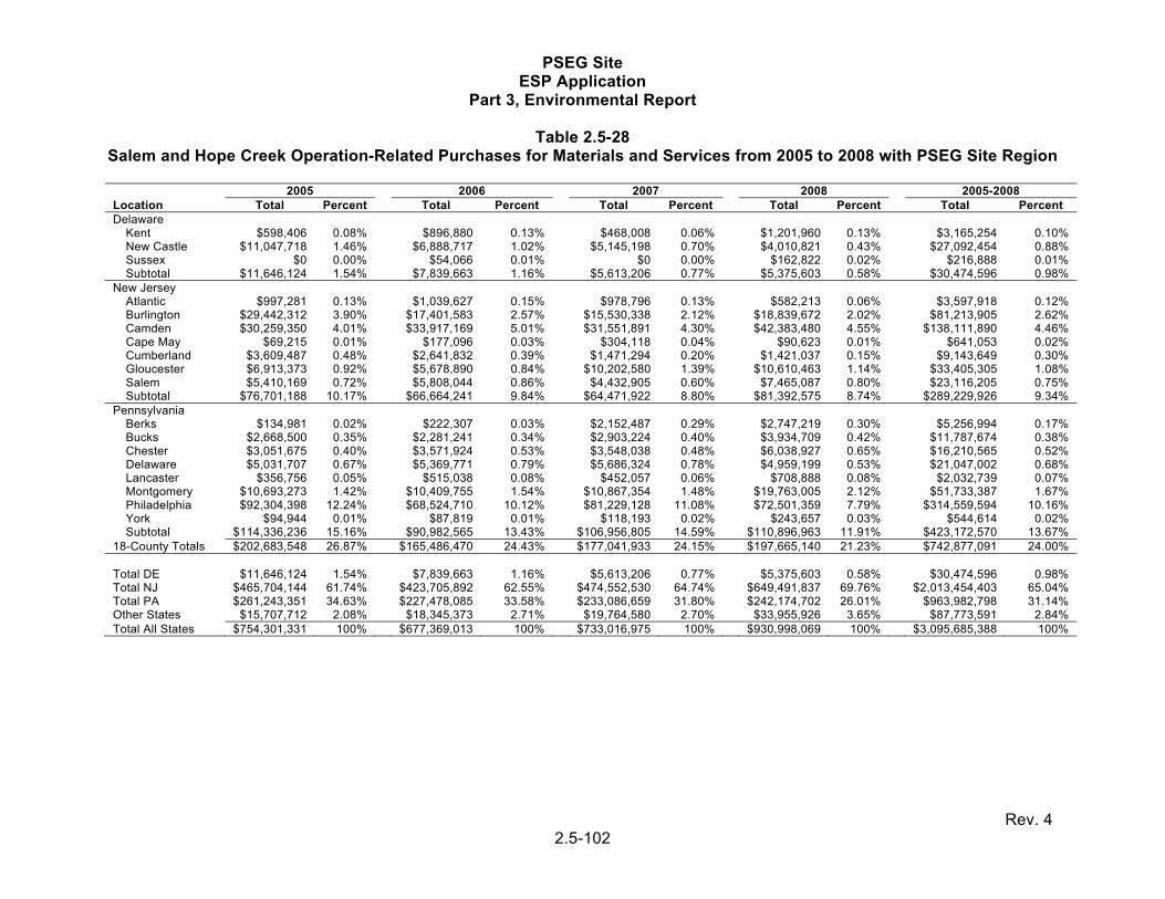
PSEG Site ESP Application
Part 3, Environmental Report
Rev. 4 2.5-102
Table 2.5-28 Salem and Hope Creek Operation-Related Purchases for Materials and Services from 2005 to 2008 with PSEG Site Region
Location 2005 2006 2007 2008 2005-2008
Total Percent Total Percent Total Percent Total Percent Total Percent Delaware
Kent $598,406 0.08% $896,880 0.13% $468,008 0.06% $1,201,960 0.13% $3,165,254 0.10% New Castle $11,047,718 1.46% $6,888,717 1.02% $5,145,198 0.70% $4,010,821 0.43% $27,092,454 0.88% Sussex $0 0.00% $54,066 0.01% $0 0.00% $162,822 0.02% $216,888 0.01% Subtotal $11,646,124 1.54% $7,839,663 1.16% $5,613,206 0.77% $5,375,603 0.58% $30,474,596 0.98%
New Jersey Atlantic $997,281 0.13% $1,039,627 0.15% $978,796 0.13% $582,213 0.06% $3,597,918 0.12% Burlington $29,442,312 3.90% $17,401,583 2.57% $15,530,338 2.12% $18,839,672 2.02% $81,213,905 2.62% Camden $30,259,350 4.01% $33,917,169 5.01% $31,551,891 4.30% $42,383,480 4.55% $138,111,890 4.46% Cape May $69,215 0.01% $177,096 0.03% $304,118 0.04% $90,623 0.01% $641,053 0.02% Cumberland $3,609,487 0.48% $2,641,832 0.39% $1,471,294 0.20% $1,421,037 0.15% $9,143,649 0.30% Gloucester $6,913,373 0.92% $5,678,890 0.84% $10,202,580 1.39% $10,610,463 1.14% $33,405,305 1.08% Salem $5,410,169 0.72% $5,808,044 0.86% $4,432,905 0.60% $7,465,087 0.80% $23,116,205 0.75% Subtotal $76,701,188 10.17% $66,664,241 9.84% $64,471,922 8.80% $81,392,575 8.74% $289,229,926 9.34%
Pennsylvania Berks $134,981 0.02% $222,307 0.03% $2,152,487 0.29% $2,747,219 0.30% $5,256,994 0.17% Bucks $2,668,500 0.35% $2,281,241 0.34% $2,903,224 0.40% $3,934,709 0.42% $11,787,674 0.38% Chester $3,051,675 0.40% $3,571,924 0.53% $3,548,038 0.48% $6,038,927 0.65% $16,210,565 0.52% Delaware $5,031,707 0.67% $5,369,771 0.79% $5,686,324 0.78% $4,959,199 0.53% $21,047,002 0.68% Lancaster $356,756 0.05% $515,038 0.08% $452,057 0.06% $708,888 0.08% $2,032,739 0.07% Montgomery $10,693,273 1.42% $10,409,755 1.54% $10,867,354 1.48% $19,763,005 2.12% $51,733,387 1.67% Philadelphia $92,304,398 12.24% $68,524,710 10.12% $81,229,128 11.08% $72,501,359 7.79% $314,559,594 10.16% York $94,944 0.01% $87,819 0.01% $118,193 0.02% $243,657 0.03% $544,614 0.02% Subtotal $114,336,236 15.16% $90,982,565 13.43% $106,956,805 14.59% $110,896,963 11.91% $423,172,570 13.67%
18-County Totals $202,683,548 26.87% $165,486,470 24.43% $177,041,933 24.15% $197,665,140 21.23% $742,877,091 24.00% Total DE $11,646,124 1.54% $7,839,663 1.16% $5,613,206 0.77% $5,375,603 0.58% $30,474,596 0.98% Total NJ $465,704,144 61.74% $423,705,892 62.55% $474,552,530 64.74% $649,491,837 69.76% $2,013,454,403 65.04% Total PA $261,243,351 34.63% $227,478,085 33.58% $233,086,659 31.80% $242,174,702 26.01% $963,982,798 31.14% Other States $15,707,712 2.08% $18,345,373 2.71% $19,764,580 2.70% $33,955,926 3.65% $87,773,591 2.84% Total All States $754,301,331 100% $677,369,013 100% $733,016,975 100% $930,998,069 100% $3,095,685,388 100%

PSEG Site ESP Application
Part 3, Environmental Report
Rev. 4 2.5-103
Table 2.5-29 Corporate, Income, Property, and Sales Tax Rates for 2008 for States and Region of Influence Counties within a 50-Mile
Radius of the PSEG Site
Location
Percent of 2005-2008
PSEG Payroll(a)
Percent of 2005-2008
PSEG Purchases(b)
Tax Rates (in Percent)
Corporate Income Property
Sales County Local
Delaware 18.4 0.98 NA 0.5 – 5.95 0
New Castle 18.3 0.5614 1.8635-3.5267
New Jersey 70.6 65 9 1.4 – 8.97 7
Cumberland 9.9 3.025-4.888
Gloucester 15.1 2.199-6.251
Salem 38.1 1.033-6.190 Lower Alloways Creek
Township
1.033
Salem City 3.339
Pennsylvania 8.2 31.1 NA 3.07 6
References 2.5-25, 2.5-87, 2.5-103, and 2.5-104
a) Values from Table 2.5-17 b) Values from Table 2.5-28

PSEG Site ESP Application
Part 3, Environmental Report
Rev. 4 2.5-104
Table 2.5-30 Personal Income for 25 Counties within 50 Miles of the PSEG Site and
Four-County Region of Influence, 1990 to 2007
Years Average Annual
1990 2000 2007 Growth (%) Delaware
New Castle County $23,810 $34,751 $45,755 3.9% Three County Average(a) $19,087 $27,585 $35,993 3.8%
State Average(a) $21,422 $30,871 $40,112 3.8%
Maryland
Seven County Average $20,420 $31,356 $43,216 4.5%
State Average $22,852 $34,264 $46,471 4.3%
New Jersey
Cumberland County $17,295 $23,375 $29,599 3.2%
Gloucester County $18,830 $28,027 $37,331 4.1%
Salem County $19,165 $27,672 $35,236 3.6%
Seven County Average $20,185 $29,545 $37,698 3.7%
State Average $24,572 $38,377 $49,511 4.2%
Pennsylvania
Eight County Average $22,810 $34,802 $44,598 4.0%
State Average $19,687 $29,698 $38,793 4.1% a) Three County Average and State Average values as given in reference Reference2.5-112

PSEG Site ESP Application
Part 3, Environmental Report
Rev. 4 2.5-105
Table 2.5-31 Housing Information for Counties within 50 Miles of the PSEG Site, 1990 to 2007
1990 2000 2005 to 2007(a)
Overall Growth (%)
Delaware (Three-County Total)
Total Housing Units 289,919 343,072 382,149 31.8%
Occupied 247,497 298,736 321,748 30.0%
Owner-Occupied 173,896 216,038 236,646 36.1%
Renter-Occupied 73,601 82,698 85,102 15.6%
Vacant Units 42,422 44,336 60,401 42.4%
Median value (dollars) NA 124,167 215,667 73.7%
Maryland (Seven-County Total)
Total Housing Units 423,222 485,953 511,636 20.9%
Occupied 398,049 459,152 480,117 20.6%
Owner-Occupied 273,998 324,765 343,535 25.4%
Renter-Occupied 124,051 134,387 136,582 10.1%
Vacant Units 25,173 26,801 31,519 25.2%
Median value (dollars) NA 133,686 278,333 108.2%
New Jersey (Seven-County Total)
Total Housing Units 683,897 740,202 789,408 15.4
Occupied 588,048 641,442 680,395 15.7
Owner-Occupied 421,110 467,521 502,165 19.2
Renter-Occupied 166,938 173,921 178,230 6.8
Vacant Units 95,849 98,760 109,013 13.7
Median value (dollars) 117,814 216,674 83.9
Pennsylvania (Eight-County Total)
Total Housing Units 1,917,015 2,052,573 2,135,781 11.4%
Occupied 1,790,479 1,921,468 1,956,507 9.3%
Owner-Occupied 1,242,176 1,337,662 1,373,314 10.6%
Renter-Occupied 548,303 583,806 583,193 6.4%
Vacant Units 126,536 131,105 179,274 41.7%
Median value (dollars) NA 128,700 217,688 69.1% NA-Not Available
a) Based on three year interim reporting period between census dates Reference 2.5-123

PSEG Site ESP Application
Part 3, Environmental Report
Rev. 4 2.5-106
Table 2.5-32 Housing Information for Four-County Region of Influence of the PSEG Site,
1990 to 2007
1990 2000 2005-2007 Overall Growth
(%)
New Castle County, DE Total Housing Units 173,560 199,521 211,073 21.6% Occupied 164,161 188,935 193,434 17.8%
Owner-Occupied 112,122 132,514 138,742 23.7% Renter-Occupied 52,039 56,421 54,692 5.1%
Vacant Units 9399 10,586 17,639 87.7% Rental Units NA 6216 10,586 70.3% Median Monthly Rent (dollars) NA 593 764 28.8% Median value (dollars) 136,000 237,400 74.6%
Cumberland County, NJ Total Housing Units 50,294 52,863 54,749 8.9% Occupied 47,118 49,143 50,165 6.5%
Owner-Occupied 32,276 33,389 34,322 6.3% Renter-Occupied 14,842 15,754 15,843 6.7%
Vacant Units 3176 3720 4584 44.3% Rental Units NA 2269 2278 0.4% Median Monthly Rent (dollars) NA 518 620 19.7% Median value (dollars) 91,200 156,500 71.6%
Gloucester County, NJ Total Housing Units 82,459 95,054 105,426 27.9% Occupied 78,845 90,717 99,708 26.5%
Owner-Occupied 61,736 72,516 81,213 31.5% Renter-Occupied 17,109 18,201 18,495 8.1%
Vacant Units 3614 4337 5718 58.2% Rental Units NA 2462 3034 23.2% Median Monthly Rent (dollars) NA 557 734 31.8% Median value (dollars) 120,100 220,400 83.5%
Salem County, NJ Total Housing Units 25,349 26,158 27,313 7.7% Occupied 23,794 24,295 25,073 5.4%
Owner-Occupied 17,203 17,724 18,825 9.4% Renter-Occupied 6591 6571 6248 -5.2%
Vacant Units 1555 1863 2240 44.1% Rental Units NA 814 685 -15.8% Median Monthly Rent (dollars) NA 516 674 30.6% Median value (dollars) 105,200 173,600 65.0%
NA-Not Available
Reference 2.5-123

PSEG Site ESP Application
Part 3, Environmental Report
Rev. 4 2.5-107
Table 2.5-33 School Enrollments and Capacities within 50 Miles of the PSEG Site, 2008
Location Number
of Schools Total
Enrollments Average
Enrollment
Unused Capacity
(%)(a)
Delaware (Three Counties) High School 36 31,462 874 18.6 Middle School 40 23,760 594 16.3 Elementary School 103 49,387 479 20.5 Subtotals 179 104,609 584 19.0
Maryland (Seven Counties) High School 21 23,290 1109 4.4 Middle School 23 15,796 687 20.5 Elementary School 69 33,447 485 4.1 Subtotals 113 72,533 642 8.3
New Jersey (Seven Counties) High School 74 75,644 1022 NA Middle School 95 49,388 520 NA Elementary School 271 111,373 411 NA Subtotals 440 236,405 537
Pennsylvania (Eight Counties) High School 132 133,068 1008 NA Middle School 166 96,416 581 NA Elementary School 346 188,951 546 NA Subtotals 644 418,435 650
Region Totals High School 263 263,464 1002 Middle School 324 185,360 572 Elementary School 789 383,158 486 All Schools 1376 831,982 605
References: 2.5-6, 2.5-13, 2.5-19, 2.5-39, 2.5-54, 2.5-59, 2.5-70, 2.5-85, and 2.5-101
a) Capacity figures are based on 149 schools in Delaware and 113 schools in Maryland. No school capacity data was found for New Jersey and Pennsylvania schools.

PSEG Site ESP Application
Part 3, Environmental Report
Rev. 4 2.5-108
Table 2.5-34 School Enrollments and Capacities in the PSEG Site Four-County Region of Influence
Location
Number of
Schools Total
Enrollments Average
Enrollment
Unused Capacity
(%)(a)
New Castle County, DE High School 24 20,863 869 21.3% Middle School 31 16,622 536 29.4% Elementary School 72 36,441 506 20.0% Totals 127 73,926 582 22.8%
Cumberland County, NJ High School 7 7706 1101 NA Middle School 11 4125 375 NA Elementary School 39 14,848 381 NA Totals 57 26,679 468
Gloucester County, NJ High School 14 14,442 1032 NA Middle School 17 11,452 674 NA Elementary School 54 23,799 441 NA Totals 85 49,693 585
Salem County, NJ High School 7 3764 538 NA Middle School 12 2812 234 NA Elementary School 20 5561 278 NA Totals 39 12,137 311
References 2.5-19, 2.5-70, and 2.5-101
a) Capacity figures were only available for 50 schools in DE

PSEG Site ESP Application
Part 3, Environmental Report
Rev. 4 2.5-109
Table 2.5-35 Colleges and Universities within 50 Miles of the PSEG Site and Four-County
Region of Influence
Total Enrollments Number Institutions(a) Enrollments
Within 50 Miles Delaware (3 counties) 48,039 9 Maryland (7 counties) 10,565 3 Harford Community College 5841New Jersey (7 counties) 57,820 11 Pennsylvania (8
counties) 219,865 53Community College of
Philadelphia 17,334 Drexel University 20,682 Temple University 35,489 University of Pennsylvania 23,980Total 336,289 76
Total Enrollments Number Institutions(b) Enrollments
Region of Influence New Castle County, DE 38,690 6 University of Delaware 20,352 Wilmington University 8353
Delaware Technical/Community
College 7519Salem County, NJ 1306 1 Cumberland County College 3822Cumberland County, NJ 3822 1 Rowan University 9770Gloucester County, NJ 15,906 2 Gloucester County College 6135 Salem Community College 1306Total 59,724 10
a) Includes only major institutions with enrollments greater than 5,000 b) All institutions
References 2.5-4, 2.5-7, 2.5-14, 2.5-91, 2.5-92, 2.5-106, 2.5-110, and 2.5-111

PSEG Site ESP Application
Part 3, Environmental Report
Rev. 4 2.5-110
Table 2.5-36 Refuges, Trusts and Parks within 50 Miles of PSEG Site
Location Total Acres
National Wildlife Refuges
National Trust / Preserves Private Parks State Parks
# Acres # Acres # Acres # Acres
Delaware
New Castle 7403 0 0 0 0 0 0 11 7403
3 Counties 33,447 2 25,978 0 0 0 0 12 7469
Maryland
7 Counties 39,711 2 2287 1 400 3 25,900 6 11,124
New Jersey
Cumberland 7756 0 0 2 7756 0 0 0 0
Gloucester 0 0 0 0 0 0 0 0 0
Salem 17,775 1 4600 1 609 0 0 4 12,566
7 Counties 217,197 2 15,600 3 8365 0 0 8 193,231
Pennsylvania
8 Counties 17,775 3 3700 17 4357 0 0 6 9718
Total 308,130 9 47,565 21 13,122 3 25,900 32 221,542 References 2.5-2, 2.5-8, 2.5-12, 2.5-30, 2.5-40, 2.5-42, 2.5-56, 2.5-57, 2.5-58, 2.5-66, 2.5-72, 2.5-73, 2.5-84, 2.5-132, 2.5-135, 2.5-136, and 2.5-137 Note: The data for the four counties in the Region of Influence are shaded.

PSEG Site ESP Application
Part 3, Environmental Report
Rev. 4 2.5-111
Table 2.5-37 Taxes Paid by PSEG for the Hope Creek and Salem Generating Stations, and Energy and
Environmental Resource Center
Taxing Authority Year 2005 to 2009
Type of Tax 2005 2006 2007 2008 2009 Total
Salem City
Property Tax $220,822 $228,492 $318,910 $265,276 $387,353 $1, 420,853
Salem City Total Tax Revenues $6,294,613 $6,485,947 $7,389,319 $8,474,461 $8,364,553 $37,008,893
PSEG Percent of Total Tax Revenues 3.5% 3.5% 4.3% 3.1% 4.6% 3.8%
Lower Alloways Creek Township
Property Tax $1,269,268 $1,191,870 $1,253,019 $1,168,202 $1,512,997 $6,395,356
Township Total Tax Revenues $2,325,378 $2,195,746 $2,310,262 $2,145,098 $2,789,386 $11,765,870
PSEG Percent of Total Tax Revenues 54.6% 54.3% 54.2% 54.5% 54.2% 54.4%
Other New Jersey Townships
Property Tax
Elsinboro $30,607 $33,021 $34,932 $38,754 $40,194 $177,508
Hopewell $4547 $4906 $5190 $9541 $9378 $33,562
Greenwich $102,400 $110,477 $116,869 $118,124 $117,105 $564,975
Fairfield $17,652 $19,044 $20,146 $34,989 $26,097 $117,928
Dennis $7563 $8160 $8632 $9071 $9385 $42,811
Commercial $66,137 $71,354 $75,482 $80,279 $69,384 $362,636
Maurice River $11,458 $12,362 $13,077 $14,002 $14,255 $65,154
Lower Alloways Creek $8259 $8910 $9426 $2328 $756 $29,679
Total for Other Townships $248,623 $268,234 $283,754 $307,088 $286,554 $1,394,253
Total $1,738,713 $1,688,596 $1,855,683 $1,740,566 $2,186,904 $9,210,462 Salem County
County Total Tax Revenues $40,562,971 $43,382,037 $46,667,551 $50,139,854 $51,302,437 $232,054,850
PSEG Percent of Total Tax Revenues(a) 3.7% 3.3% 3.4% 2.9% 3.7% 3.4%

PSEG Site ESP Application
Part 3, Environmental Report
Rev. 4 2.5-112
Table 2.5-38 (Sheet 1 of 2) Major Water Suppliers (Serving 5000 or More People) within PSEG Site Region of Influence
Water System Name Population
Served
Primary Water
Source
Total Daily Capacity
(Mgd)
Peak Daily Demand
(Mgd)
Demand as a % of Capacity
Excess Capacity
(Mgd)
Excess as a % of Capacity
Delaware - New Castle County Artesian Water Company, Inc. 215,100 Wells 27 NA NA NA NACity of Wilmington Water 140,000 Surface 61 29 47.5% 32 52.5%Tidewater Utilities, Inc. 30,000 Ground NA NA NA NA NAUnited Water Delaware 105,270 Surface 6 2.5 41.7% 3.5 58.3%New Castle Water Department 6000 Ground 1.3 0.5 38.5% 0.8 61.5%Middletown Water Department 9900 Ground NA NA NA NA NANewark Water Department 36,130 Surface 6 4 66.7% 2 33.3%Total or Average 542,400 101.3 36 35.5%
Total or Average Excess (4 providers)
287,400 74.3 36 48.5% 38.3 51.5%
New Jersey
Cumberland County Bridgeton Water Department 22,770 Ground 3.31 4.06 122.7% -0.75 -22.7%Millville Water & Sewer Utility 27,500 Ground 7.24 6.37 88.0% 0.87 12.0%Vineland Water & Sewer Utility 33,000 Ground 16.39 15.08 92.0% 1.31 8.0%Subtotal or Average 83,270 26.95 25.52 94.7% 1.43 5.3%
Gloucester County Clayton Water Department 7155 Ground 1.94 1.06 54.6% 0.88 45.4%Deptford Municipal Water Authority 26,000 Purchased
Surface 8.60 4.72 54.9% 3.88 45.1%
Glassboro Water Department 19,238 Ground 6.04 4.13 68.4% 1.91 31.6%Greenwich Water Department 4921 Ground 1.73 1.30 74.9% 0.43 25.1%Mantua Municipal Water Authority 11,713 Ground 2.38 2.33 98.2% 0.04 1.8%Monroe Municipal Water Authority 26,145 Ground 7.15 6.22 86.9% 0.94 13.1%NJ American Water Company -
Logan 5967 Ground 2.15 1.66 77.5% 0.48 22.5%
Paulsboro Water Department 6200 Ground 1.80 1.25 69.3% 0.55 30.7%Pitman Water Department 9445 Ground 1.59 0.96 60.1% 0.64 39.9%

PSEG Site ESP Application
Part 3, Environmental Report
Rev. 4 2.5-113
Table 2.5-38 (Sheet 2 of 2) Major Water Suppliers (Serving 5000 or more People) within PSEG Site Region of Influence
Water System Name Population
Served
Primary Water
Source
Total Daily Capacity
(Mgd)
Peak Daily Demand
(Mgd)
Demand as a % of Capacity
Excess Capacity
(Mgd)
Excess as a % of Capacity
Gloucester County (cont’d) NJ American Water Company -
Harrison 9450 Ground 3.80 3.80 100.0% 0.00 0.0%
Washington Municipal Water Authority 48,000 Ground 12.92 8.25 63.9% 4.67 36.1%
West Deptford Water Department 20,000 Ground 7.03 4.21 59.9% 2.82 40.1% Westville Water Department 6000 Ground 1.73 0.70 40.3% 1.03 59.7%
Woodbury Water Department 11,000 Purchased
surface 4.32 1.76 40.6% 2.57 59.4%
Subtotal or Average 211,234 63.18 42.34 67.0% 20.84 33.0% Salem County
Pennsville Water Department 13,500 Ground 1.87 1.63 87.1% 0.24 12.9% Hope Creek Water Department 6199 Ground 4.27 1.66 38.7% 2.62 61.3% Subtotal 19,699 6.15 3.29 53.5% 2.86 46.5%
Gloucester/Salem Shared Penns Grove Water Supply
Company 14,406 Ground 2.6 2.0 74.5% 0.67 25.5%
Total or Average 328,609 99 73.1 73.9% Total or Average Excess 25.8 26.1%
References 2.5-22, 2.5-23, 2.5-26, and 2.5-71

PSEG Site ESP Application
Part 3, Environmental Report
Rev. 4 2.5-114
Table 2.5-39 Public Wastewater Treatment Systems in Four-County Region of Influence of PSEG Site
Waste Water Treatment Plants Population
Served
Total Capacity
(Mgd)
Average Daily Usage
(Mgd)
Usage as a % of Total Capacity
Excess Capacity
(Mgd)
Excess as a % of total Capacity
(Mgd) New Castle, DE
Wilmington STP 503,708 102.8 71.2 69.3% 31.5 30.7% Delaware City STP 1879 0.50 0.25 50.0% 0.25 50.0% Port Penn STP 262 0.05 0.04 80.0% 0.01 20.0% Subtotal or Average 505,849 103.3 71.5 69.2% 31.8 30.8%
Cumberland, NJ Cumberland Co. UA-Cohansey RV STP 22,771 7.00 3.41 48.7% 3.59 51.3% Landis Sewerage Authority 34,307 8.20 5.36 65.4% 2.84 34.6% City of Millville STP 26,847 5.00 2.59 51.8% 2.41 48.2% Subtotal or Average 83,925 20.2 11.4 56.2% 8.84 43.8%
Gloucester, NJ Gloucester County Utilities Authority NA 24.1 17.2 71.4% 6.90 28.6% Greenwich Township STP 4511 1.00 0.91 91.0% 0.09 9.0% Harrison Township STP 6246 0.40 0.31 77.5% 0.09 22.5% Logan Township MUA 6032 1.20 0.59 49.2% 0.61 50.8% Swedesboro Consolidated STP 2008 0.35 0.27 77.1% 0.08 22.9% Subtotal or Average 18,797 27.1 19.3 71.2% 7.77 28.8%
Salem, NJ Carney's pt. TWP SA 7597 1.30 0.72 55.4% 0.58 44.6% Penns Grove SA 4840 0.75 0.66 88.0% 0.09 12.0% Pennsville SA 12,083 1.88 1.58 84.0% 0.30 16.0% Salem City STP 5793 1.40 0.86 61.4% 0.54 38.6% Woodstown STP 3260 0.50 0.30 60.0% 0.20 40.0% Lower Alloways Creek-Leisure Arms
STP 231 0.02 0.01 50.0% 0.01 50.0% Lower Alloways Creek-Hancock STP 817 0.05 0.02 40.0% 0.03 60.0% Lower Alloways Creek-Canton STP 772 0.05 0.02 40.0% 0.03 60.0% Subtotal or Average 35,393 5.95 4.17 70.1% 1.78 29.9%
Total or Average for Four-County Region of Influence 643,964 156.5 106.3 67.9% 50.2 32.1%
Reference 2.5-130

PSEG Site ESP Application
Part 3, Environmental Report
Rev. 4 2.5-115
Table 2.5-40 Police and Fire Personnel within 50 Miles of the PSEG Site and
Four-County Region of Influence
Location Police
Personnel
Residents Per
Officer Fire
Personnel
Residents Per
Firefighter
Delaware New Castle 1101 478 1649 319 Three Counties 1780 484 4040 213
Maryland Seven Counties 2969 424 9513 132
New Jersey Cumberland 402 387 797 195 Gloucester 343 832 1326 215 Salem 273 241 605 109 Seven Counties 3245 566 8823 208
Pennsylvania Eight Counties 9855 528 19,057 273
References 2.5-32, 2.5-33, 2.5-36, and 2.5-131
Note: The data for the four counties in the Region of Influence are shaded.

PSEG Site ESP Application
Part 3, Environmental Report
Rev. 4 2.5-116
Table 2.5-41 Physicians and Hospital Beds within 50 Miles of the PSEG Site and
Four-County Region of Influence
Location PhysiciansPhysicians Per 1000 Residents
Hospital Beds
Hospital BedsPer 1000
Residents
Delaware New Castle 1708 3.3 1166 2.2 Three Counties 2325 2.7 1955 2.3
Maryland Seven Counties 4765 3.8 1836 1.5
New Jersey Cumberland 217 1.4 409 2.7 Gloucester 321 1.1 240 0.9 Salem 75 1.1 110 1.7 Seven Counties 4460 2.4 4086 2.2
Pennsylvania Eight Counties 20,582 4.0 15,723 3.0
Reference 2.5-123
Note: The data for the four counties in the Region of Influence are shaded.
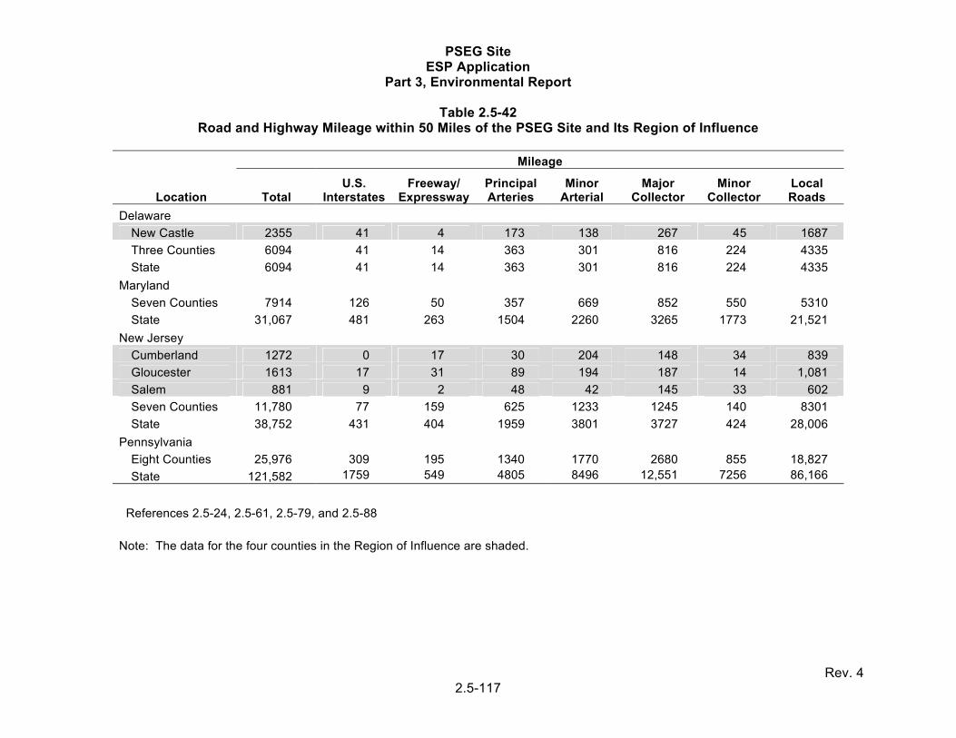
PSEG Site ESP Application
Part 3, Environmental Report
Rev. 4 2.5-117
Table 2.5-42 Road and Highway Mileage within 50 Miles of the PSEG Site and Its Region of Influence
Location
Mileage
Total U.S.
InterstatesFreeway/
ExpresswayPrincipal Arteries
Minor Arterial
Major Collector
Minor Collector
Local Roads
Delaware
New Castle 2355 41 4 173 138 267 45 1687
Three Counties 6094 41 14 363 301 816 224 4335
State 6094 41 14 363 301 816 224 4335
Maryland
Seven Counties 7914 126 50 357 669 852 550 5310
State 31,067 481 263 1504 2260 3265 1773 21,521
New Jersey
Cumberland 1272 0 17 30 204 148 34 839
Gloucester 1613 17 31 89 194 187 14 1,081
Salem 881 9 2 48 42 145 33 602
Seven Counties 11,780 77 159 625 1233 1245 140 8301
State 38,752 431 404 1959 3801 3727 424 28,006
Pennsylvania
Eight Counties 25,976 309 195 1340 1770 2680 855 18,827
State 121,582 1759 549 4805 8496 12,551 7256 86,166
References 2.5-24, 2.5-61, 2.5-79, and 2.5-88
Note: The data for the four counties in the Region of Influence are shaded.

PSEG Site ESP Application
Part 3, Environmental Report
Rev. 4 2.5-118
Table 2.5-43 Annual Average Daily Traffic Counts on Roads in Proximity to the PSEG Site
Annual Average
Daily Traffic (AADT) Year Roadway and Location
NJ 49, between NJ 45 and York Street 12,920 2005
NJ 45, between CR 657 and Howell Street 8748 2007 Alloway Creek Neck Road, between Grosscup Road and Pancoast Road 3175 2007
Fort Elfsborg Road, between CR 627 and Mason Point 351 2005
Money Island Road, just south of CR 627 403 2006 Chestnut Street, between Grieves Pkwy and Maple Avenue 1787 2008 Grieves Parkway, between CR 625 (Chestnut) and CR 665 (Walnut) 3342 2007
Oak Street, between Chestnut Street and Wesley Street 1324 2007
Reference 2.5-81

PSEG Site ESP Application
Part 3, Environmental Report
Rev. 4 2.5-119
Table 2.5-44 International and General Aviation Airports within 50 Miles of the PSEG Site
Airport Name County Closest City State Type of Airport
New Castle Airport New Castle Wilmington DE Business Airport of Local Impact
Delaware Airpark Kent Cheswold DE General Aviation Airport(a)
Summit Airport New Castle Middletown DE General Aviation Airport
Millville Municipal Airport
Cumberland Millville NJ General Aviation Airport
Philadelphia International Airport
Philadelphia Philadelphia PA Business Airport of Regional Impact
Brandywine Airport Chester West Chester PA General Aviation Airport
Chester County G.O. Carlson Airport
Chester Coatesville PA General Aviation Airport
New Garden Airport Chester Toughkenamon PA General Aviation Airport
Wings Field Montgomery Blue Bell PA General Aviation Airport
Reference 2.5-34
a) General aviation (GA) is one of two categories of civil aviation. It refers to all flights other than military and scheduled airline flights, both private and commercial.

PSEG Site ESP Application
Part 3, Environmental Report
Rev. 4 2.5-120
Table 2.5-45
Identified Historic Properties Located in the Proposed Causeway and Parking Areas
State Site Number
Site Components Eligibility
28SA179 Mid 18th to 19th Century, Middle to Late Woodland Period
Both components potentially eligible
28SA180 18th to 19th Century, Middle to Late Woodland Period
Both components potentially eligible
28SA181 18th to 19th Century, Middle to Late Woodland Period
Historic component potentially eligible
28SA182 18th to 19th Century, Middle to Late Woodland Period
Both components potentially eligible
28SA183 18th to 19th Century, Middle to Late Woodland Period
Both components potentially eligible
28SA186 18th to 19th Century Historic component potentially eligible
Reference 2.5-46

PSEG Site ESP Application
Part 3, Environmental Report
Rev. 4 2.5-121
Table 2.5-46 (Sheet 1 of 5) Historic Properties Listed on the NRHP Located within a 10-Mile Radius of the PSEG Site
Name Address City County StateDistance from
PSEG Site (mi.) Joseph Ware House 134 Poplar Street Hancock's Bridge
Area Salem NJ 3.9
Alloways Creek Friends Meetinghouse
Buttonwood Ave, 150 ft. west of Main Street
Hancock's Bridge Salem NJ 4.9
Hancock House Route 49 and Front Street Lower Alloways Creek Township
Salem NJ 5.1
Hedge-Carpenter-Thompson Historic District
Bounded by Hedge, Thompson, South Third streets and Oak Street Alley
Salem Salem NJ 8.1
Broadway Historic District Broadway from Front to Yorke Street Salem Salem NJ 8.2 Market Street Historic District Market Street from Broadway to Fenwick
Creek Salem Salem NJ 8.5
Abel and Mary Nicholson House Junction of Hancock's Bridge and Fort Elfsborg Road
Elsinboro Area Salem NJ 4.8
Sarah and Samuel Nicholson House
2 mi. south of Salem on Amwellbury Road Salem Area Salem NJ 5.4
Benjamin Holmes House West of Salem on Fort Elfsborg-Hancock's Bridge Road
Salem Area Salem NJ 5.8
Fort Mott and Finns Point National Cemetery District
Northwest of Salem on Fort Mott Road Salem Area Salem NJ 9.8
Short's Landing Hotel Complex Northeast of Smyrna Smyrna Area Kent DE 8.0 Thomas Sutton House DE 79, with Woodland Beach Wildlife
Area Woodland Beach
Area Kent DE 9.6
Liston Range Front Lighthouse 1600 Belts Road Bay View Beach New Castle DE 3.3 Old Union Methodist Church 0.2 mi. north of Blackbird Crossroads on
U.S. 13 Blackbird
Crossroads New Castle DE 8.6
Fort Dupont Historic District DE 9, South of C&D Canal Delaware City New Castle DE 7.9 Delaware City Historic District Roughly bounded by the Delaware River,
Dragon Creek, DE 9, and the C&D Canal Delaware City New Castle DE 8.4
Eastern Lock of the C&D Canal Battery Park Delaware City New Castle DE 8.4 Chelsea DE 9 Delaware City New Castle DE 8.6

PSEG Site ESP Application
Part 3, Environmental Report
Rev. 4 2.5-122
Table 2.5-46 (Sheet 2 of 5) Historic Properties Listed on the NRHP Located within a 10-Mile Radius of the PSEG Site
Name Address City County StateDistance from
PSEG Site (mi.) Fort Delaware on Pea Patch Island
Pea Patch Island in the Delaware River Delaware City New Castle DE 8.9
Fairview U.S. 13 Delaware City Area New Castle DE 8.1 Philip Reading Tannery 201 East Main Street Middletown New Castle DE 9.4 Middletown Academy 218 North Broad Street Middletown New Castle DE 9.7 Middletown Historic District Roughly bounded by Redding, Scott,
Lockwood, and Catherine streets Middletown New Castle DE 9.7
St. Joseph's Church 15 West Cochran Street Middletown New Castle DE 9.7 Greenlawn North Broad Street Middletown New Castle DE 9.8 Okolona Route 429 Middletown Area New Castle DE 5.2 Belleview Route 428 Middletown Area New Castle DE 7.3 Noxontown South of Middletown off DE 896 Middletown Area New Castle DE 8.1 Pharo House Odessa and Silver Lake Roads Middletown Area New Castle DE 8.6 Maple Grove Farm Route 299 Middletown Area New Castle DE 8.9 Achmester North of Middletown on SR 429 Middletown Area New Castle DE 9.3 Weston Off DE 71 Middletown Area New Castle DE 9.4 Arnold S. Naudain House South of Middletown on DE 71 Middletown Area New Castle DE 9.5 Old St. Anne's Church South of Middletown off DE 71 Middletown Area New Castle DE 9.6 Idalia Manor Route 13 Mt. Pleasant Area New Castle DE 8.1 Old Drawyers Church U.S. 13 Odessa New Castle DE 6.3 Odessa Historic District Roughly Main and High streets between
Appoquinimink River and DE 4 Odessa New Castle DE 6.5
Corbit-Sharp House Southwest corner of Main and 2nd streets Odessa New Castle DE 6.6 Old St. Paul's Methodist Episcopal Church
High Street Odessa New Castle DE 6.6
Appoquinimink Friends Meetinghouse
Main Street Odessa New Castle DE 6.9
A. M. Vail House Rt. 299 Odessa New Castle DE 8.8 Hell Island Site Address Restricted Odessa Area New Castle DE 3.5

PSEG Site ESP Application
Part 3, Environmental Report
Rev. 4 2.5-123
Table 2.5-46 (Sheet 3 of 5) Historic Properties Listed on the NRHP Located within a 10-Mile Radius of the PSEG Site
Name Address City County StateDistance from
PSEG Site (mi.) Riverdale Off Bay View and Silver Run roads Odessa Area New Castle DE 3.9 Green Meadow Thomas Landing Road (DE 440),
Appoquinimink Hundred Odessa Area New Castle DE 4.3
David W. Thomas House 326 Thomas Landing Road, Appoquinimink Hundred
Odessa Area New Castle DE 4.8
J. M. Gordon House Route 44 Odessa Area New Castle DE 4.8 J. Vandegrift House Route 44 Odessa Area New Castle DE 5.1 S. Higgins Farm Route 423 Odessa Area New Castle DE 5.4 Misty Vale Route 423 Odessa Area New Castle DE 5.8 Monterey North of Odessa on Bayview Road Odessa Area New Castle DE 6.1 Fairview Southeast of Odessa Odessa Area New Castle DE 6.2 Comdr. Thomas MacDonough House
North of Odessa on U.S. 13 Odessa Area New Castle DE 6.5
Elm Grange U.S. 13 Odessa Area New Castle DE 6.6 Retirement Farm U.S. 13 Odessa Area New Castle DE 6.8 Mondamon Farm Route 2 Odessa Area New Castle DE 7.0 Hill Island Farm 3379 Dupont Parkway (U.S. 13),
Appoquinimink Hundred Odessa Area New Castle DE 7.3
Williams House 1.2 mi. northwest of Odessa on Marl Pit Road
Odessa Area New Castle DE 7.8
Duncan Beard Site Address Restricted Odessa Area New Castle DE 8.0 Old Ford Dairy U.S. 13 Odessa Area New Castle DE 8.1 Sereck Shallcross House West of Odessa off U.S. 13 Odessa Area New Castle DE 8.3 J. K. Williams House DE 4 Odessa Area New Castle DE 8.4 McWhorter House Route 412 Odessa Area New Castle DE 8.7 Fairview Route 412 Odessa Area New Castle DE 9.2 Port Penn Historic District DE 9 Port Penn New Castle DE 4.2 Augustine Beach Hotel South of Port Penn on DE 9 Port Penn Area New Castle DE 3.9 Robert Grose House 1000 Port Penn Road Port Penn Area New Castle DE 5.1

PSEG Site ESP Application
Part 3, Environmental Report
Rev. 4 2.5-124
Table 2.5-46 (Sheet 4 of 5) Historic Properties Listed on the NRHP Located within a 10-Mile Radius of the PSEG Site
Name Address City County StateDistance from
PSEG Site (mi.) Dilworth House Off DE 9 Port Penn Area New Castle DE 5.3 Ashton Historic District North of Port Penn on Thornton Road Port Penn Area New Castle DE 5.4 Hazel Glen West of Port Penn on DE 420 Port Penn Area New Castle DE 5.5 Cleaver House Off Biddle's Corner Road Port Penn Area New Castle DE 6.0 Liston Ranger Rear Light Station West of Port Penn on DE 2 Port Penn Area New Castle DE 7.0 John B. Nelson House West of Port Penn off U.S. 13 Port Penn Area New Castle DE 7.1 Windsor 1060 Dutch Neck Road, St. Georges
Hundred Port Penn Area New Castle DE 7.1
Fleming House Northeast of Smyrna on DE 9 Smyrna Area New Castle DE 7.6 Sutton House Broad and Delaware streets St. Georges New Castle DE 8.8 Vernacular Frame House Delaware Street St. Georges New Castle DE 8.8 North Saint Georges Historic District
Roughly along Main, Broad, Delaware and Church streets, Red Lion Hundred
St. Georges New Castle DE 8.9
St. Georges Presbyterian Church
Main Street St. Georges New Castle DE 8.9
Biddle House South of St. Georges on U.S. 13 St. Georges Area New Castle DE 7.3 Bloomfield U.S. 13 St. Georges Area New Castle DE 9.1 Linden Hill U.S. 13 St. Georges Area New Castle DE 9.4 St. Georges Cemetery Caretaker's House
Kirkwood and St. Georges Rd. St. Georges Area New Castle DE 9.8
Hart House East of Taylors Bridge on DE 453 Taylors Bridge Area New Castle DE 4.1 Liston House East of Taylors Bridge on DE 453 Taylors Bridge Area New Castle DE 4.1 Johnson Home Farm CR 453 east of junction with DE 9,
Blackbird Hundred Taylors Bridge Area New Castle DE 4.4
Reedy Island Range Rear Light Junction of DE 9 and Road 453 Taylors Bridge Area New Castle DE 4.9

PSEG Site ESP Application
Part 3, Environmental Report
Rev. 4 2.5-125
Table 2.5-46 (Sheet 5 of 5) Historic Properties Listed on the NRHP Located within a 10-Mile Radius of the PSEG Site
Name Address City County StateDistance from
PSEG Site (mi.) Huguenot House West of Taylors Bridge on DE 9 Taylors Bridge Area New Castle DE 6.1 Townsend Historic District Roughly bounded by Gray, Ginn and
South, Lattamus and Main streets and Commerce Street and Cannery Lane and Railroad Avenue
Townsend New Castle DE 9.7
Reference 2.5-65

PSEG Site ESP Application
Part 3, Environmental Report
Rev. 4 2.5-126
Table 2.5-47 Environmental Justice Populations(a) within 50-Mile Radius of the PSEG Site
State/County Nu
mb
er
of
Blo
ck
Gro
up
s
Bla
ck
Am
eri
ca
n I
nd
ian
o
r N
ati
ve
Ala
sk
an
As
ian
Na
tiv
e H
aw
aii
an
or
Oth
er
Pa
cif
ic
Isla
nd
er
So
me
Oth
er
Ra
ce
Mu
ltir
ac
ial
Ag
gre
ga
te
His
pa
nic
Lo
w-I
nc
om
e
Ho
us
eh
old
s
Delaware Kent 69 6 0 0 0 0 0 10 0 1New Castle 352 70 0 0 0 7 1 74 13 21Sussex 21 2 0 0 0 0 0 2 1 0
Maryland Baltimore 70 7 0 0 0 0 0 10 0 1Caroline 17 2 0 0 0 0 0 2 1 0Cecil 55 0 0 0 0 0 0 0 0 1Harford 138 2 0 0 0 0 0 7 2 2Kent 19 0 0 0 0 0 0 0 0 0Queen
Anne's 16 0 0 0 0 0 0 0 0 0Talbot 2 0 0 0 0 0 0 0 0 0
New Jersey Atlantic 52 2 0 0 0 0 0 2 3 0Burlington 136 0 0 0 0 0 0 1 0 0Camden 407 89 0 3 0 28 0 103 40 47Cape May 53 2 0 0 0 0 0 2 0 0Cumberland 100 12 0 0 0 10 0 23 14 9Gloucester 196 16 0 0 0 0 0 11 0 4Salem 49 9 0 0 0 0 0 7 1 2
Pennsylvania Berks 2 0 0 0 0 0 0 0 0 0Bucks 2 0 0 0 0 0 0 0 0 0Chester 248 15 0 1 0 1 0 21 8 6Delaware 463 83 0 7 0 1 0 96 2 13Lancaster 46 0 0 0 0 0 0 0 0 0Montgomery 326 35 0 1 0 0 0 41 5 3Philadelphia 1770 980 1 73 0 141 9 1171 195 556York 7 0 0 0 0 0 0 0 0 0
Total 4616 1332 1 85 0 188 10 1583 285 666 Percentage of State Population
Delaware 783,600 19.0 0.4 2.0 0.0 2.1 1.8 25.4 4.8 8.8Maryland 5,296,486 27.7 0.3 4.0 0.0 1.8 2.1 36.0 4.3 8.3New Jersey 8,414,350 13.4 0.2 5.7 0.0 5.4 2.7 27.5 13.3 8.3Pennsylvania 12,281,054 9.9 0.2 1.8 0.0 1.5 1.3 14.6 3.2 11.0
a) Number of block groups that meet NRC criteria for minority and/or low-income populations (NRC, 2004) Note: Shaded counties are completely within the 50-mile radius References 2.5-119, 2.5-124, and 2.5-124

PSEG Site ESP Application
Part 3, Environmental Report
Rev. 4 2.5-127
Table 2.5-48 Environmental Justice Populations for Selected Counties(a) within 50-Mile Radius of the PSEG Site
County
Block Groups with Environmental Justice Populations(b)
Total Block Groups Black Asian Other Multiracial Aggregate Hispanic Low-Income
Household
#
Blocks % of Total
# Blocks
% of Total
# Blocks
% of Total
# Blocks
% of Total
# Blocks
% of Total
# Blocks
% of Total
# Blocks
% of Total
# Blocks
% of Total
Delaware New Castle 352 7.6% 70 5.3% 0 0.0% 7 3.7% 1 10.0% 74 4.7% 13 4.6% 21 3.2%
New Jersey Camden 407 8.8% 89 6.7% 3 3.5% 28 14.9% 0 0.0% 103 6.5% 40 14.0% 47 7.1% Cumberland 100 2.2% 12 0.9% 0 0.0% 10 5.3% 0 0.0% 23 1.5% 14 4.9% 9 1.4% Gloucester 196 4.2% 16 1.2% 0 0.0% 0 0.0% 0 0.0% 11 0.7% 0 0.0% 4 0.6% Salem 49 1.1% 9 0.7% 0 0.0% 0 0.0% 0 0.0% 7 0.4% 1 0.4% 2 0.3%
Pennsylvania Chester 248 5.4% 15 1.1% 1 1.2% 1 0.5% 0 0.0% 21 1.3% 8 2.8% 6 0.9% Delaware 463 10.0% 83 6.2% 7 8.2% 1 0.5% 0 0.0% 96 6.1% 2 0.7% 13 2.0% Montgomery 326 7.1% 35 2.6% 1 1.2% 0 0.0% 0 0.0% 41 2.6% 5 1.8% 3 0.5% Philadelphia 1770 38.3% 980 73.6% 73 85.9% 141 75.0% 9 90.0% 1171 74.0% 195 68.4% 556 83.5%
All Others 705 15.3% 23 1.7% 0 0.0% 0 0.0% 0 0.0% 36 2.3% 7 2.5% 5 0.8% Total 4616 1332 85 188 10 1583 285 666 a) Includes counties within the four-county Region of Influence and counties containing more than 200 minority block groups b)"American Indian or Native Alaskan" and "Native Hawaiian or Other Pacific Islander excluded from table due to poor representation within 50-mile radius (Table 2.5.4-1) Shaded counties comprise the socioeconomic Region of Influence. References 2.5-119 and 2.5-124

PSEG Site ESP Application
Part 3, Environmental Report
Rev. 4 2.5-128
Table 2.5-49 Population Trends in the 50-Mile Region(a)
County
Total Population White Black Asian All Other Minorities Hispanic Family-Poverty 2000 2005-2007 2000 2005-2007 2000 2005-2007 2000 2005-2007 2000 2005-2007 2000 2005-2007 2000 2005-
2007 Delaware
Kent 126,697 147,974 73.5% 71.3% 20.7% 21.2% 1.7% 2.2% 4.1% 5.3% 3.2% 4.1% 8.1% 8.8% New Castle 500,265 524,682 73.1% 70.8% 20.2% 22.4% 2.6% 3.6% 4.1% 3.2% 5.3% 6.9% 5.6% 6.4%
New Jersey Cumberland 146,438 154,086 65.9% 66.9% 20.2% 20.8% 1.0% 1.1% 12.9% 11.2% 19.0% 22.7% 11.3% 13.4% Gloucester 254,673 281,218 87.1% 84.8% 9.1% 9.6% 1.5% 2.2% 2.3% 3.4% 2.6% 3.5% 4.3% 5.4% Salem 64,285 65,789 81.2% 80.2% 14.8% 15.5% 0.6% 0.5% 3.4% 3.8% 3.9% 4.9% 7.2% 6.3% Atlantic 252,552 269,774 68.4% 65.9% 17.6% 16.3% 5.1% 6.4% 8.9% 11.4% 12.2% 14.1% 7.6% 7.8% Camden 508,932 513,147 70.9% 66.7% 18.1% 18.7% 3.7% 4.5% 7.3% 10.1% 9.7% 11.7% 8.1% 8.8% Cape May 102,326 97,555 91.6% 91.0% 5.1% 5.9% 0.6% 0.2% 2.7% 2.9% 3.3% 4.1% 6.4% 6.7%
Maryland Caroline 29,772 32,240 81.7% 81.4% 14.8% 13.5% 0.5% 0.8% 3.0% 4.3% 2.7% 4.2% 9.0% 8.6% Cecil 85,951 98,358 93.4% 91.4% 3.9% 5.1% 0.7% 1.2% 2.0% 2.3% 1.5% 2.1% 5.4% 6.6% Harford 218,590 238,960 86.8% 83.3% 9.3% 11.4% 1.5% 1.9% 2.4% 3.4% 1.9% 2.5% 3.6% 3.9% Queen Anne's 40,563 45,826 89.0% 88.9% 8.8% 8.4% 0.6% 1.0% 1.6% 1.7% 1.1% 1.8% 4.4% 4.6%
Pennsylvania Chester 433,501 478,821 89.2% 87.6% 6.2% 6.4% 2.0% 3.0% 2.6% 3.0% 3.7% 4.5% 3.1% 3.6% Delaware 550,864 553,511 80.3% 75.8% 14.5% 17.8% 3.3% 4.3% 1.9% 2.1% 1.5% 2.0% 5.8% 6.7% Montgomery 750,097 774,424 86.5% 84.3% 7.5% 8.1% 4.0% 5.2% 2.0% 2.4% 2.0% 2.9% 2.8% 3.2% Philadelphia 1,517,550 1,454,382 45.0% 42.7% 43.2% 43.8% 4.5% 5.4% 7.3% 8.1% 8.5% 10.3% 18.4% 19.3%
Totals 4,956,094 5,058,091 3,947,844 3,948,929 1,181,582 1,233,207 182,570 234,316 (355,903) (358,362) 326,063 407,485 Proportional Totals 79.7% 78.1% 23.8% 24.4% 3.7% 4.6% -7.2% -7.1% 6.6% 8.1% Net Growth 101,997 1085 51,625 51,746 (2459) 81,422 Percent Growth 2.06% 0.027% 4.4% 28.3% 0.7% 25.0% U.S. Totals 281,421,906 298,757,310 211,347,851 221,379,167 34,614,894 37,045,906 10,131,189 12,846,564 25,327,972 27,485,673 35,177,738 43,917,325 U.S. Proportional 75.1% 74.1% 12.3% 12.4% 3.6% 4.3% 9.0% 9.2% 12.5% 14.7% 9.2% 9.8% U.S. Net Growth 17,335,404 10,031,315 2,431,012 2,715,376 2,157,701 8,739,586 U.S. Percent Growth 6.16% 4.7% 7.02% 26.8% 8.5% 24.8% Region of Influence(b) 465,396 501,093 736,216 765,794 163,323 186,773 18,677 27,099 47,445 46,109 63,466 84,247 Proportional 158.2% 152.8% 35.1% 37.3% 4.0% 5.4% 10.2% 9.2% 13.6% 16.8% Net Growth 29,578 23,449 8422 (1336) 20,781 Percent Growth 4.0% 14.36% 45.1% -2.8% 32.7% a) Includes counties with half or more of area within the 50-mile radius, (no ACS data for Kent County, Maryland) b) Region of Influence includes New Castle County (DE), and Cumberland, Gloucester, and Salem counties (NJ) Note: Shaded counties comprise the socioeconomic Region of Influence Reference 2.5-119

PSEG Site ESP Application
Part 3, Environmental Report
Rev. 4 2.5-129
Table 2.5-50 Population Trends in 10-County Delaware Valley Regional Planning Commission
(DVRPC) Region
1980 2000 1980 to 2000
Race Number Percent Number Percent Net Change %
Change
White 4,286,104 79.1% 4,235,397 71.9% -50,707 -1.2%
Black 999,086 18.4% 1,176,651 20.0% 177,565 17.8%
Asian/Pacific Islander 53,605 1.0% 203,770 3.5% 150,165 280.1%
Other 83,040 1.5% 271,854 4.6% 188,814 227.4%
Total 5,421,835 5,887,672 465,837 8.6%
Hispanic 135,021 2.5% 314,598 5.3% 179,577 133.0% Reference 2.5-29

PSEG Site ESP Application
Part 3, Environmental Report
Rev. 4 2.5-130
Table 2.5-51
Farms that Employ Migrant Labor in the 50-Mile Region(a)
County
Total Farms
Farms with Hired Labor
Number of Hired
Laborers
Farms with Migrant
Labor
Delaware 2546 647 3223 75Kent 825 169 996 22New Castle 347 81 565 10
Maryland 12,834 3508 14,938 236Caroline 574 153 681 13Cecil 583 128 1110 5Harford 704 155 579 12
Kent 377 111 729 8Queen Anne's 521 126 587 13
New Jersey 10,327 2415 24,385 470
Atlantic 499 163 5924 78Camden 225 52 656 17Cape May 201 46 358 8Cumberland 615 192 3716 70Gloucester 669 163 2191 60Salem 759 172 1407 36
Pennsylvania 63,163 11,722 60,721 811Chester 1733 580 7708 101Delaware 79 25 228 2Montgomery 719 155 888 14Philadelphia 17 5 (D) 0
a) Includes counties with half or more of area within the 50-mile radius Note: Shaded counties are included with four-county Region of Influence (D) = withheld to avoid disclosing data for individual farms Reference 2.5-126

PSEG Site ESP Application
Part 3, Environmental Report
Rev. 4 2.5-131
Table 2.5-52 Farms that Employ Migrant Labor for Selected Counties in New Jersey
Atlantic Cumberland Gloucester Salem4-County
Total
New Jersey
Total
Total Farms 499 615 669 759 2542 10,327
% Farms in State 4.8% 6.0% 6.5% 7.3% 24.6%
Land in Farms (acres) 30,372 69,489 46,662 96,530 243,053 733,450
% Farm Land in State 4.1% 9.5% 6.4% 13.2% 33.1%
Farms Hiring Labor 163 192 163 172 690 2415
% Farms Hiring Labor 6.7% 8.0% 6.7% 7.1% 28.6%
Number of Laborers 5924 3716 2191 1407 13,238 24,385
% Laborers in State 24.3% 15.2% 9.0% 5.8% 54.3% Farms Hiring Migrant Labor 78 70 59 36 243 470
% Farms with Migrant Labor 16.5% 14.9% 12.6% 7.7% 51.7%
Note: Shaded counties are included with four-county Region of Influence.
Reference 2.5-126

PSEG Site ESP Application
Part 3, Environmental Report
Rev. 4 2.5-132
Table 2.5-53 Minority Farm Operators in the 50-Mile Region(a)
County All(b) All Non-
White% Non-
WhiteBlack
OperatorsAsian
Operators Hispanic
Operators
Delaware 3894 127 3.26% 27 36 35
Kent 1243 15 1.21% 4 3 3
New Castle 540 22 4.07% 9 2 11
Maryland 19,917 727 3.65% 223 139 144
Caroline 831 29 3.49% 11 4 8
Cecil 919 20 2.18% 1 0 9
Harford 1113 19 1.71% 4 0 5
Kent 570 9 1.58% 1 1 1
Queen Anne's 800 21 2.63% 1 7 0
New Jersey 16,143 544 3.37% 92 147 207
Atlantic 798 30 3.76% 1 3 24
Camden 353 29 8.22% 13 7 6
Cape May 290 6 2.07% 4 0 1
Cumberland 900 35 3.89% 13 1 10
Gloucester 1070 44 4.11% 17 4 12
Salem 1156 30 2.60% 6 8 9
Pennsylvania 93,316 1239 1.33% 101 100 526
Chester 2734 68 2.49% 8 5 46
Delaware 120 1 0.83% 1 0 0
Montgomery 1081 17 1.57% 2 2 6
Philadelphia 26 5 19.23% 2 0 2
a) Includes counties with half or more of area within the 50-mile radius b) Data was collected for a maximum of three operators per farm Note: Shaded counties are included with four-county Region of Influence Reference 2.5-126

PSEG Site ESP Application
Part 3, Environmental Report
Rev. 4 2.5-133
Table 2.5-54 Ambient Noise Levels at the HCGS and SGS in February 2009
Monitoring Location
Location Specific Attributes Noise Levels (dBA) Day Leq Night Leq
1 Open Area 500 ft. South of SGS Switchyard near Delaware River Shoreline
58.9 57.4
2 Open Area near Meteorological Tower 51.6 51.6 3 Open Area Adjacent to High-use On-site
Road 54.3 65.6
4 Open Area under 500 kV Transmission Line
53.2 53.6
5 Open Area near HCGS Cooling Tower, Small Arms Firing Range, and low-use on-site road
60.9 61.5
6 Open Area near Delaware River Shoreline 43.4 51.6 7 Open Area near Material Services
Building, HCGS Intake Pump House and Delaware River Shoreline
52.0 51.6
Notes: Leq is the true equivalent sound level measured over the run time.
Refer to Figure 2.5-17 for the positions of the seven monitoring locations.
PSEG Site ESP Application
Part 3, Environmental Report
Rev. 4 2.6-1
2.6 GEOLOGY This section provides a description of the geologic conditions at and in the vicinity of the PSEG Site. Section 2.5 of the ESPA SSAR presents a detailed site geologic evaluation. 2.6.1 GEOLOGIC SETTING The PSEG Site lies within the Coastal Plain physiographic province. This province is in the subaerial portion of the North American continental shelf. Within 200 mi. of the PSEG Site, the Coastal Plain province extends eastward from the fall line to the Atlantic Ocean along the length of the North American Atlantic margin (Figure 2.6-1). The fall line marks the area where the upland region (continental bedrock) and a coastal plain (coastal alluvia) meet. The Coastal Plain province is characterized by low-lying, gently rolling terrain developed on sequences of deltaic, shallow marine and continental shelf sediments consisting primarily of unconsolidated to semi-consolidated gravels, sands, silts, and clays that dip gently oceanward. The land surface has been modified by erosional and depositional landforms associated with several cyclical changes in sea level and varies from flat to deeply incised. However, the Coastal Plain province generally exhibits lower topographic relief than the Piedmont province to the west. The PSEG Site lies within the Outer Coastal Plain physiographic subprovince. The Middle Coastal Plain Terrace subprovince resides outside the site boundary to the east. The Middle Coastal Plain Terraces and the Upland Sands and Gravels subprovinces lie east of the PSEG Site. West-central and south-central portions of the PSEG Site are bordered by the Delaware River channel. (Figure 2.6-2) Coastal Plain sediments ranging in age from Early Cretaceous to Holocene underlie the PSEG Site. These sediments overlie a basement complex composed of fractured continental crust. The regional stratigraphic column is shown in Figure 2.6-3. Regional geologic maps (Figure 2.6-4) depict the geologic setting for the PSEG Site region. Borings completed as part of this ESP are shown on Figure 2.6-5, and the stratigraphic column (inferred from the site borings) for the PSEG Site (Figure 2.6-6) is discussed in the following subsections. Subsection 2.6.1.1 describes the PSEG Site stratigraphy. Subsection 2.6.2.1.2 describes the local stratigraphic units and geologic formations.
2.6.2 PSEG SITE STRATIGRAPHY As part of the ESP, 16 geotechnical borings were completed at the PSEG Site. Figure 2.6-5 shows the locations of these borings and identifies the locations of geologic cross-sections discussed later in this subsection. Integration and comparison of the regional geologic stratigraphy and geotechnical boring logs provide the basis for developing the site-specific stratigraphic model at the PSEG Site. Fourteen stratigraphic layers, most of which can be correlated to the regional geologic strata, are identified in the borings. The stratigraphic layers encountered during the ESPA exploration at the PSEG Site (Figure 2.6-6) are grouped into the following four periods according to geologic age (from oldest to youngest):
PSEG Site ESP Application
Part 3, Environmental Report
Rev. 4 2.6-2
Cretaceous (Lower and Upper) Paleogene (Lower Tertiary) Neogene (Upper Tertiary) Quaternary (Pleistocene and Holocene)
Stratigraphic cross-sections (Figures 2.6-7 and 2.6-8), and a surface contour map of the top of the Vincentown Formation (Figure 2.6-9), illustrate the stratigraphy and subsurface conditions at the PSEG Site. The following subsection provides a description of stratigraphic units present that fall within each of the geologic time periods listed above. 2.6.2.1.1 PSEG Site Stratigraphic Units and Geologic Formations Several stratigraphic units are recognized within each of the categories listed in Subsection 2.6.2.1. Descriptions are provided for stratigraphic units that lie within 500 to 600 ft. of the surface, within a depth range considered to be of greater importance in evaluating geologic conditions in the vicinity of the site. The following is a description of these units as they relate to the PSEG Site. The Lower Cretaceous strata encountered during the geotechnical investigation at the PSEG Site is composed of a single unit, the Potomac Formation, which is recognized in only the deepest borings performed during the investigation. This unit forms the base of the shallow subsurface (less than 500 ft.) profile at the site. The Upper Cretaceous strata encountered during the geotechnical investigation at the PSEG Site is composed of the following eight formations, listed from oldest to youngest:
Magothy Formation Merchantville Formation Woodbury Formation Englishtown Formation Marshalltown Formation Wenonah Formation Mount Laurel Formation Navesink Formation
The Paleogene strata (Lower Tertiary) encountered during the ESPA investigation at the PSEG Site is composed of two formations, listed from oldest to youngest:
Hornerstown Formation (Lower Tertiary and Upper Cretaceous) Vincentown Formation
The Neogene strata (Upper Tertiary) encountered during the geotechnical investigation at the PSEG Site is composed of the Kirkwood Formation. The Kirkwood Formation is subdivided at the site into upper and lower units based on variations in lithology. The Quaternary strata encountered during the ESPA investigation at the PSEG Site is composed of two stratigraphic units, listed from oldest to youngest:

PSEG Site ESP Application
Part 3, Environmental Report
Rev. 4 2.6-3
Alluvium Artificial and Hydraulic Fill
Subsection 2.6.2.1.2 provides detailed geologic material descriptions. 2.6.2.1.2 Description of PSEG Site Stratigraphic Units and Geologic Formations The 14 major stratigraphic layers defining the shallow subsurface profile at the PSEG Site occur between the ground surface and 631.5 ft. below ground surface (elevation -615.0 ft. NAVD). The site stratigraphic layers and geologic formations are described and characterized in the following subsections, from the Potomac Formation (oldest formation encountered) to the ground surface (Figures 2.6-6 through 2.6-8). 2.6.2.1.2.1 Cretaceous Strata
2.6.2.1.2.1.1 Potomac Formation The Potomac Formation is the deepest stratigraphic unit encountered by the ESPA borings at the PSEG Site. The Potomac Formation consists of Lower Cretaceous age non-marine, continentally-derived sediments deposited in multichanneled fluvial to deltaic environments (Reference 2.6-15). Two borings penetrated the top of the Potomac Formation during the geotechnical investigation. The top of the formation is at approximate elevation -454 ft. NAVD in the northern portion of the site, and at approximate elevation -484 ft. NAVD in the eastern portion of the site. These two borings are along a southeasterly line, in the regional dip direction. The vertical elevation difference corresponds to an apparent southeasterly dip of approximately 34 ft/mi (less than 1 percent). This is consistent with the gentle dip reported for the NJ Coastal Plain in SSAR Subsection 2.5.1.1. At the PSEG Site, the top of the Potomac Formation is interpreted from the geophysical testing conducted in the two deepest borings completed as part of the ESPA investigation. The borings are compared to and correlated with published geophysical logs from the region (References 2.6-14 and 2.6-1) to aid in identification of the top of the stratigraphic unit. Sediments in the upper portion of the Potomac Formation are typically dark gray to gray clay and sand with variable silt content. In the deeper portion of the formation, the sediments are typically mottled gray and red clay. No borings encountered the bottom of the Potomac Formation during the ESPA investigation. 2.6.2.1.2.1.2 Magothy Formation The Magothy Formation unconformably overlies the Potomac Formation and consists of Upper Cretaceous age non-marine and marine sediments deposited in fluvial to marginal marine environments (Reference 2.6-15). The two deep borings performed during the ESPA investigation penetrated the top of the Magothy Formation at approximate elevation -402 ft. NAVD, in the northern portion of the PSEG Site, and at approximate elevation -429 ft. NAVD in the eastern portion of the site. This corresponds to an apparent southeasterly dip of approximately 30 ft/mi. Borings showed the unit to range from 52 to 55 ft. thick. Sediments of the Magothy Formation typically consist of gray to very dark gray, carbonaceous/lignitic clay and
PSEG Site ESP Application
Part 3, Environmental Report
Rev. 4 2.6-4
silt at the top of the unit, interbedded with sands with variable silt and clay content at the bottom of the unit. The Magothy Formation is distinguished from the underlying Potomac Formation by comparing and correlating the geophysical logs for the two deep borings, completed as part of the ESPA investigation, with published geophysical logs from the region (References 2.6-14 and 2.6-1). 2.6.2.1.2.1.3 Merchantville Formation The Merchantville Formation conformably overlies the Magothy Formation. This formation consists of Upper Cretaceous age marine sediments deposited in a neritic or shallow marine environment during a marine transgression, as described in Subsection 2.5.1.1.3.4.1 of the SSAR. The two deep borings performed during the ESPA investigation penetrated the top of the Merchantville Formation at approximate elevation -372 ft. NAVD in the northern portion of the PSEG Site, and at approximate elevation -398 ft. NAVD in the eastern portion of the site. This corresponds to an apparent southeasterly dip of approximately 29 ft/mi. The unit is approximately 30 ft. thick. Sediments of the Merchantville Formation consist of greenish-black to black, glauconitic silt and clay with trace to some fine sand and trace mica; locally with trace friable to moderately indurated layers. Content of glauconite, considered indicative of a continental shelf marine depositional environment with a slow rate of accumulation, ranged from trace to little. The Merchantville Formation is distinguished from the overlying Woodbury Formation by the increase in glauconite content, and general decrease in plasticity and mica content. 2.6.2.1.2.1.4 Woodbury Formation The Woodbury Formation conformably overlies the Merchantville Formation. This formation consists of Upper Cretaceous age marine sediments deposited in an inner shelf environment associated with a marine regression (Reference 2.6-11). Two deep borings penetrated the top of the unit during the ESPA investigation at approximate elevation -336 ft. NAVD in the northern portion of the site, and at approximate elevation -368 ft. NAVD in the eastern portion of the site. This corresponds to an apparent southeasterly dip of approximately 36 ft/mi. The thickness of the Woodbury Formation ranges from 30 to 36 ft. across the PSEG Site. Sediments of the Woodbury Formation consist of very dark gray and black to greenish-black, highly plastic clay with trace glauconite, fine sand, mica, and shell fragments; and locally with trace indurated layers. Sediments of the Woodbury Formation are very similar to those of the overlying Englishtown Formation, and the two formations appear to have a gradational contact. The results of the geophysical logging reveal little difference in natural gamma response or resistivity between these two units, or with the underlying Merchantville Formation. 2.6.2.1.2.1.5 Englishtown Formation The Englishtown Formation conformably overlies the Woodbury Formation and consists of Upper Cretaceous age marine sediments deposited in a near-shore environment associated with a marine regression, as described in Subsection 2.5.1.1.3.4.1 of the SSAR. Five borings were advanced to the top of the unit during the ESPA investigation, at approximate elevation -

PSEG Site ESP Application
Part 3, Environmental Report
Rev. 4 2.6-5
291 ft. NAVD in the northern portion of the site, and at approximate elevation -319 ft. NAVD in the eastern portion of the site. This corresponds to an apparent southeasterly dip of approximately 32 ft/mi. The thickness of the Englishtown Formation ranges from 44 to 49 ft. across the PSEG Site. Sediments in the upper portion of the Englishtown Formation consist of micaceous, very dark greenish-gray to very dark gray and black sandy silt and clay to clayey sand, with trace shell fragments and trace to little glauconite. Sediments grade downward into micaceous, black, highly plastic silt and clay with trace to few fine sand and trace shell fragments. 2.6.2.1.2.1.6 Marshalltown Formation The Marshalltown Formation conformably overlies the Englishtown Formation and consists of Upper Cretaceous age marine sediments deposited in a neritic environment during a marine transgression as described in SSAR Subsection 2.5.1.1.3.4.1. Five borings penetrated the top of the Marshalltown Formation during the ESPA investigation at elevations ranging from -265 to -277 ft. NAVD in the northern portion of the PSEG Site, and at approximate elevation -293 ft. NAVD in the eastern portion of the site. This corresponds to an apparent southeasterly dip of approximately 29 ft/mi. The Marshalltown Formation is approximately 25 ft. thick across the PSEG Site. Sediments of this unit typically consist of greenish-gray to very dark gray and black, clayey and silty, fine to medium sand, and fine sandy clay of variable plasticity, all with trace to little glauconite content. Trace amounts of shell fragments, pyrite nodules, friable layers, and subrounded fine gravel were locally encountered within the Marshalltown Formation. 2.6.2.1.2.1.7 Wenonah Formation The Wenonah Formation conformably overlies the Marshalltown Formation. This formation consists of Upper Cretaceous age marine sediments deposited in a neritic environment during a marine regression (Reference 2.6-11). Six borings penetrated the top of the formation during the ESPA investigation. The top of the Wenonah Formation was encountered at elevations ranging from -250 to -259 ft. NAVD in the northern portion of the PSEG Site, and at approximate elevations ranging from -279 to -289 ft. NAVD in the eastern portion of the PSEG Site. This corresponds to an apparent southeasterly dip of approximately 33 ft/mi. The Wenonah Formation has an average thickness of approximately 15 ft. across the PSEG Site. The formation typically consists of very dark gray to greenish-black, sandy clay with trace shell fragments and trace to few glauconite fragments. Locally, the formation consists of clayey and silty, fine to medium sand with trace to few glauconite fragments. 2.6.2.1.2.1.8 Mount Laurel Formation The Mount Laurel Formation conformably overlies the Wenonah Formation and consists of Upper Cretaceous age marine sediments deposited in a near-shore environment during a marine regression (Reference 2.6-11). All geotechnical borings penetrated the top of the formation during the ESPA investigation. The top of the Mount Laurel Formation was encountered at elevations ranging from -145 to -157 ft. NAVD in the northern portion of the PSEG Site, and at approximate elevations ranging from 168 to -177 ft. NAVD in the eastern portion of the PSEG Site. This corresponds to an apparent southeasterly dip of approximately 26 ft/mi. The unit has an average thickness of 103 ft. in the northern portion of the site,

PSEG Site ESP Application
Part 3, Environmental Report
Rev. 4 2.6-6
thickening slightly to the southeast, with an average thickness of 111 ft. in the eastern portion of the site. Sediments of the Mount Laurel Formation typically consist of dark olive-gray, dark grayish- brown, and greenish-gray, clayey and silty, fine to medium sand, grading with depth into fine to medium sand with variable silt and clay content, all with trace to little glauconite, and shell fragments. The amount of glauconite and shell fragments was found to decrease to trace amounts with increasing depth. The upper 15 to 20 ft. of the formation typically contains trace to little subrounded, coarse sand and fine gravel, and is locally composed of sandy clay. 2.6.2.1.2.1.9 Navesink Formation The Navesink Formation conformably overlies the Mount Laurel Formation. This formation consists of Upper Cretaceous age marine sediments deposited in a neritic environment during a marine transgression (Reference 2.6-11). The top of the Navesink Formation is encountered at elevations ranging from -121 to -133 ft. NAVD in the northern portion of the PSEG Site, and at approximate elevations ranging from -147 to -157 ft. NAVD in the eastern portion of the PSEG Site. This corresponds to an apparent southeasterly dip of approximately 31 ft/mi. The thickness of the unit averages 24 ft. in the northern portion of the site, thinning slightly to the southeast, with an average thickness of 20 ft. in the eastern portion of the site. Sediments of the Navesink Formation are typically composed of very dark greenish-gray to very dark grayish-green and greenish-black, silty and clayey, fine to medium grained glauconite, and quartz sand with trace to little shell fragments. The Navesink Formation is a distinctive marker unit across the PSEG Site due to its composition being almost entirely glauconite. 2.6.2.1.2.2 Paleogene Strata (Lower Tertiary)
2.6.2.1.2.2.1 Hornerstown Formation The Hornerstown Formation conformably overlies the Navesink Formation and consists of Upper Cretaceous to Paleocene age marine sediments (Reference 2.6-11). The top of the Hornerstown Formation is encountered at elevations ranging from -105 to -114 ft. NAVD in the northern portion of the PSEG Site, and at approximate elevations ranging from -127 to -137 ft. NAVD in the eastern portion of the PSEG Site. This corresponds to an apparent southeasterly dip of approximately 26 ft/mi. The formation averages 20 ft. thick across the PSEG Site. Regionally, the Hornerstown Formation is described as well-sorted, almost purely glauconitic sand that imparts a distinctive green color to the unit (Reference 2.6-11). At the PSEG Site, the sediments of the Hornerstown Formation are typically composed of greenish-gray to very dark greenish-gray, silty and clayey, fine to medium sand, with trace to few shell fragments, and trace to some glauconite. Glauconite content typically increases with depth and is estimated from field sample observations to comprise greater than 30 percent of the sand fraction near the base of the formation. The formation contains numerous, discontinuous, friable to indurated calcium carbonate-cemented sandstone layers. These cemented zones are typically 0.1 to 1 ft. thick, as observed
PSEG Site ESP Application
Part 3, Environmental Report
Rev. 4 2.6-7
from split-spoon sampling and drilling operations. The sediments of the Hornerstown Formation are very similar to, and grade into, those of the overlying Vincentown Formation, making the units difficult to distinguish in the field. In general, the Hornerstown Formation is differentiated from the overlying Vincentown Formation on the basis of increasing silt/clay content and increasing glauconite content relative to the Vincentown Formation. 2.6.2.1.2.2.2 Vincentown Formation The Vincentown Formation serves as the bearing layer for the foundations of the existing nuclear units (Hope Creek and Salem Generating Stations) (References 2.6-12 and 2.6-13). The formation conformably overlies the Hornerstown Formation and consists of Paleocene age marine sediments deposited in a shallow marine environment as sea levels receded (Reference 2.6-11). The Vincentown Formation shows significant erosional relief on its upper surface, making both the elevation of its upper contact and its thickness somewhat variable. In the northern portion of the site, the elevation of the top of the formation ranges from -33 to -70 ft. NAVD. In the eastern portion of the PSEG Site, the elevation ranges from -40 to -91 ft. NAVD. Figure 2.6-9 illustrates the variability of the top of the Vincentown Formation in the northern portion of the site. The thickness of the Vincentown Formation ranges from 35 to 79 ft., averaging 52 ft. in the northern portion of the site. Thickness ranges from 37 to 93 ft. and averages 55 ft. in the eastern portion of the site. Due to the erosional nature of the upper surface of the Vincentown Formation, the sediments of the uppermost portion of the unit typically show signs of weathering characterized by oxidation of iron-bearing minerals such as glauconite. The weathering and oxidation of the formation is subject to the vagaries of post-depositional processes, such as subaerial exposure and fluvial erosion, prior to deposition of the overlying sediments, as well as groundwater movement through the formation. This results in distinct, but irregular contacts with the underlying unoxidized sediments that are not the result of depositional or stratigraphic control. Oxidized sediments are typically yellowish-brown to reddish-brown, and unoxidized sediments are typically light greenish-gray to dark greenish-gray. The oxidized and unoxidized Vincentown Formation sediments are typically composed of glauconitic, calcareous, silty and clayey, fine to medium sand, and fine to medium sand with variable silt content. Glauconite and shell fragments are typically present in trace amounts with locally higher concentrations observed during field sampling. The formation contains interbedded calcium carbonate-cemented sandstone layers. These layers are typically 0.1 to 1 ft. thick, as observed from split-spoon sampling and drilling operations. 2.6.2.1.2.3 Neogene Strata (Upper Tertiary)
2.6.2.1.2.3.1 Kirkwood Formation Where present, the Kirkwood Formation unconformably overlies the Vincentown Formation. This formation consists of Miocene age marine sediments deposited in a delta and shore-dominated shelf environment (Reference 2.6-15). The Kirkwood Formation rests on the erosional unconformity formed on top of the Vincentown Formation, and the upper surface of the Kirkwood Formation forms an erosional unconformity with the overlying alluvial sediments,
PSEG Site ESP Application
Part 3, Environmental Report
Rev. 4 2.6-8
making the elevation of the unit’s upper surface, as well as the thickness of the unit, somewhat variable. In the northern portion of the PSEG Site, the top of the Kirkwood Formation ranges from approximate elevations of -34 to -43 ft. NAVD. In the eastern portion of the PSEG Site, the top of the formation ranges from approximate elevations of -23 to -49 ft. NAVD. The thickness of the formation ranges from 12 to 29 ft., averaging 17 ft. in the northern portion of the site. Thickness of the Kirkwood Formation ranges from 14 to 54 ft., and averages 35 ft. in the eastern portion of the site. The large variation in thickness observed in the Kirkwood Formation is directly related to the erosional contact with the underlying Vincentown Formation, which displays up to 37 ft. of relief in the northern portion of the site, and up to 51 ft. of relief in the eastern portion of the site. Where the top of the Vincentown Formation is topographically low, the Kirkwood Formation is generally thick. Where the top of the Vincentown Formation is topographically high, the Kirkwood Formation is generally thin. The sediments of the Kirkwood Formation consist of two distinct units. The upper unit of the formation typically consists of dark gray, green, and brown to olive-gray, highly plastic clay and silt, with trace fine sand and rounded gravel, trace shell fragments, and trace to little organic content. Locally, interbeds of silty and clayey, fine to medium sand occur within this upper unit. In the eastern portion of the PSEG Site, a thick section of light greenish-gray, silty, fine to medium sand is locally encountered above the finer grained sediments. The lower, basal unit of the Kirkwood Formation typically consists of a 2 to 14 ft. thick layer composed of dark greenish-gray, olive gray, and dark gray to brown, silty and clayey, fine to medium sand and fine to coarse gravel. The sand and gravel in this lower unit is typically rounded to subangular. Six of the 16 borings completed during the ESPA investigation did not encounter the lower unit sediments of the Kirkwood Formation. This may indicate that the lower unit has some discontinuity across the site, or that the layer is thinner than the distance between the 5-ft. standard penetration test sample intervals at these locations. Boring NB-2, completed in the northern portion of the site, did not encounter the upper unit of the Kirkwood Formation. This is most likely due to fluvial scour during deposition of the overlying alluvial sediments at this location. At boring NB-7, completed in the northern portion of the PSEG Site, sediments of the Kirkwood Formation are completely absent, with alluvial sand and gravel unconformably overlying strongly oxidized Vincentown Formation sediments. This condition is most likely due to fluvial scour during deposition of the alluvial sediments at this location. 2.6.2.1.2.4 Quaternary Strata
2.6.1.1.2.4.1 Alluvium Alluvium unconformably overlies the Kirkwood Formation. This stratigraphic unit consists of Quaternary age sediments representing the bed of a former location of the Delaware River (Reference 2.6-13). The unit is typically encountered at approximate elevations ranging from -22 to -35 ft. NAVD in the northern portion of the PSEG Site, and at approximate elevations ranging from -16 to -25 ft. NAVD in the eastern portion of the site. The unit shows a slightly undulating upper surface, and generally slopes gently westward towards the Delaware River. The thickness of the Alluvium ranges from 5 to 24 ft. across the PSEG Site. Average thickness in the

PSEG Site ESP Application
Part 3, Environmental Report
Rev. 4 2.6-9
northern portion of the PSEG Site is approximately 13 ft. Average thickness in the eastern portion of the site is approximately 17 ft. Alluvial soils consist typically of gray to grayish-brown, fine to coarse sand with trace to little, rounded to angular, fine to coarse gravel, and trace to little silt and clay content. In borings completed in the northern and eastern portions of the PSEG Site, 2 to 5 ft. thick discontinuous layers of fine-grained soils, consisting of sandy silts and clays and highly organic soils consisting of peat, were locally encountered intercalated with the alluvial sand and gravel layers. In the eastern portion of the site, a 4 to 15 ft. thick discontinuous layer of non-organic silt and clay was locally encountered below the alluvial sand and gravel. Geophysical logging did not encompass sufficient portions of the Alluvium to allow an interpretation. 2.6.1.1.2.4.2 Hydraulic and Artificial Fill Hydraulic fill was deposited at the PSEG Site as the result of channel dredging of the Delaware River (Reference 2.6-13). The combined Hydraulic and Artificial Fill stratigraphic unit overlies alluvial soils at an average elevation of -29 ft. NAVD in the northern portion of the site, and at an average elevation of -21 ft. NAVD in the eastern portion of the site. Hydraulic fill consists typically of dark gray to dark greenish-gray, highly plastic clay and silt with trace to some organic material, and locally interbedded discontinuous layers of clayey and silty, fine to medium grained sand up to 5 ft. thick. Thickness of the hydraulic fill ranges from 24 to 44 ft., with an average thickness of 33 ft. across the northern and eastern portions of the site. Artificial fill comprises the surface material at the PSEG Site, overlying hydraulic fill. Artificial fill consists of typically grayish-brown to brown, silt, clay, and sand with variable silt and clay content, and clayey and silty gravels. Thickness of the artificial fill ranges from 2 to 10 ft., and averages 4 ft. across the northern and eastern portions of the site. These materials were placed at the site during previous construction activities and grade downward into the hydraulic fill. 2.6.3 REFERENCES 2.6-1 Benson, R. N., “Internal Stratigraphic Correlation of the Subsurface Potomac
Formation, New Castle County, Delaware, and Adjacent Areas in Maryland and New Jersey,” Delaware Geologic Survey Report of Investigations No. 71, 15 pp., 2006.
2.6-2 Dames & Moore, “Report of Foundation Studies, Proposed Hope Creek
Generating Station, Lower Alloways Creek Township, New Jersey Public Service Electric and Gas Company,” May 23, 1974.
2.6-3 Dames & Moore, “Report of Foundation Studies, Proposed Salem Nuclear
Generating Station, Salem, New Jersey, Public Service Electric & Gas Company,” August 28, 1968.
2.6-4 Dillon, W. P. and R. N. Oldale, “Late Quaternary Sea-Level Curve:
Reinterpretation Based on Glaciotectonic Influence,” Geology 6: 56 – 60, 1978.

PSEG Site ESP Application
Part 3, Environmental Report
Rev. 4 2.6-10
2.6-5 Fenneman, N.M. and D.W. Johnson, “Physiographic Divisions of the Conterminous U.S.,” USGS Publications, 1946.
2.6-6 Garrity, C.P. and D.R. Soller, “Database of the Geologic Map of North
America,” adapted from the map by J.C. Reed, Jr. and others (2005): U.S. Geological Survey Data Series 424, http://pubs.usgs.gov/ds/424/, 2009.
2.6-7 Hack, J. T., “Geomorphology of the Appalachian Highlands,” in “The
Appalachian – Ouachita Orogen in the United States,” in Hatcher, R. D., W. A. Thomas, and G. W. Viele, eds., The Geology of North America, The Geological Society of America, Volume F-2: 459 – 470, 1989.
2.6-8 NOT USED 2.6-9 NOT USED 2.6-10 McKenna, T.E., P.P. McLaughlin, and R.N. Benson, “Characterization of the
Potomac Aquifer, an Extremely Heterogeneous Fluvial System in the Atlantic Coastal Plain of Delaware,” in the Atlantic Coastal Plain of Delaware: Delaware Geological Survey Open File Report 45, 2004.
2.6-11 Olsson, R. K., T. G. Gibson, H. J. Hansen, and J. P. Owens, “Geology of the
Northern Atlantic Coastal Plain: Long Island to Virginia,” in R. E. Sheridan and J. A. Grow, eds., The Geology of North America, The Atlantic Continental Margin: U. S., Geological Society of America, I-2: 87 – 105, 1988.
2.6-12 Public Service Enterprise Group (PSEG), “Salem Generating Station Updated
Final Safety Analysis Report,” p. 2.4.5, February 15, 1987. 2.6-13 Public Service Enterprise Group (PSEG), “Hope Creek Generating Station
Updated Final Safety Analysis Report,” p. 2.4.5, 1988. 2.6-14 Sugarman, P.J. and D.H. Monteverde, “Correlation of Deep Aquifers Using
Coreholes and Geophysical Logs in Parts of Cumberland, Salem, Gloucester and Camden Counties, New Jersey,” New Jersey Geological Survey, Geologic Map Series 08-1, 2008.
2.6-15 Sugarman, P. J., K. G. Miller, J. V. Browning, A. A. Kulpecz, P. P. McLaughlin,
and D. H. Monteverde, “Hydrostratigraphy of the New Jersey Coastal Plain: Sequences and Facies Predict Continuity of Aquifers and Confining Units,” Stratigraphy 2(3): 259 – 275, 2005.
2.6-16 U.S. Geological Survey, “Professional Paper 1680, Plate 1,”
http://pubs.usgs.gov/pp/2005/pp1680/pdf/Plate1.pdf, accessed October 21, 2009.

PSEG Site ESP Application
Part 3, Environmental Report
Rev. 4 2.7-1
2.7 METEOROLOGY AND AIR QUALITY This section provides a meteorological description of the new plant site and surrounding climate area. The information supports independent evaluations and assessments of atmospheric diffusion characteristics and new plant impacts on the environment. The information presented here is based on the methodology and data analysis described in SSAR Section 2.3. Included are regional, local, and site specific climatological and meteorological information. 2.7.1 REGIONAL CLIMATOLOGY 2.7.1.1 Data Sources Several sources of data are used to characterize regional climatological conditions pertinent to the PSEG Site, as follows:
Thirty-two yr of data collected during the period of record 1977 through 2008 by the existing HCGS and SGS primary on-site meteorological monitoring system
Regional Cooperative Network surface observing stations for which Climatography of
the United States No. 20 summaries, Daily Surface Data DS 3200 digital datasets, or Climatography of the United States No. 81 summaries are available
Regional first-order surface observing stations for which Local Climatological Data
summaries and International Station Meteorological Climate Summary temperature joint frequency distributions (JFDs) are available
Regional hourly surface observing stations for which American Society of Heating,
Refrigerating and Air-Conditioning Engineers and Air Force Combat Climatology Center climatic design information tables are available
Tornado, waterspout, hurricane, and other weather event statistics for counties in the
area of the PSEG Site, from the National Climatic Data Center online Storm Events Database
Tracks of tropical cyclones from an NOAA Coastal Services Center historical
database, for an area within a radius of 115 nautical miles (nmi) from the PSEG Site
American Society of Civil Engineers structure design standards for the PSEG Site area
Maps of relative humidity in the PSEG Site region from the Climate Atlas of the United States
SSAR Subsection 2.3.1.4 provides explanations of the selection of primary sources of regional data used to characterize regional climatology at the PSEG Site. As described in SSAR Subsection 2.3.1.3, the region referred to here is an area surrounding the site that is determined by analysis to be representative of the site climate.

PSEG Site ESP Application
Part 3, Environmental Report
Rev. 4 2.7-2
2.7.1.2 General Climate Description The climate of the PSEG Site region is dominated by winds with offshore components (eastward components, with respect to the Atlantic Ocean shoreline) except in the immediate vicinity of the shoreline. Therefore, the regional climate has a lee shore character which allows features of a continental climate to be present over inland areas. The climate is continental in character, includes extremes, has a marine influence, and is quite changeable. SSAR Subsections 2.3.1.1 and 2.3.1.2 further describe the general climate of the new plant site. 2.7.1.3 Normal, Mean, and Extreme Regional Climatological Conditions 2.7.1.3.1 Temperature Extreme temperatures in the PSEG Site climate region range from 108 °F (at Marcus Hook, PA) to -15°F (at Millington 1 SE, NJ). Mean conditions are relatively homogeneous across the surrounding climate area. The mean annual temperature ranges from 56.8°F at Dover, DE, to 53.9°F at Hammonton 1 NE, NJ. SSAR Subsections 2.3.1.7 and 2.3.2.2.3 identify the sources and locations of the extreme and normal temperature values given above. 2.7.1.3.2 Atmospheric Water Vapor The mean annual wet bulb temperature at Wilmington, DE, is 48.9°F. Maximum monthly mean wet bulb temperature at Wilmington is 69.0°F in July, and lowest mean monthly wet bulb temperature is 29.0°F in January. Mean annual dew point temperature at Wilmington is 44.6°F. Highest and lowest mean monthly dew point temperatures at Wilmington are 66.1°F in July and 24.1°F in January. Based on 32 yr of on-site SGS and HCGS data, mean annual dew point temperature is 41.1°F and highest and lowest monthly mean dew point temperatures are 61.5°F in July and 21.0°F in January. Mean annual relative humidity values at Wilmington and the PSEG Site (based on 32 years of on-site data at HCGS and SGS) are 68 and 65.6 percent, respectively. Based on Wilmington statistics, relative humidity typically reaches a diurnal maximum during early morning (at 0700 local time) and a diurnal minimum typically during early afternoon (at 1300 local time). Mean Wilmington early morning relative humidity (at 0100 local time) exceeds 80 percent during the months of June through October. SSAR Subsection 2.3.2.2.4 presents the selection criteria and sources for the mean atmospheric water vapor values given above.

PSEG Site ESP Application
Part 3, Environmental Report
Rev. 4 2.7-3
2.7.1.3.3 Precipitation Mean annual total rainfall for the PSEG Site and its climate surroundings ranges from 36.04 in. at the site, to 46.28 in. at Dover, DE. Regional mean annual total snowfall ranges from 7.5 in. at Glassboro 2 NE, NJ, to 19.3 in. at Philadelphia International Airport in PA. Maximum recorded 24-hr. snowfall from records for regional stations is 30.7 in. at Marcus Hook, PA, on January 8, 1996. Maximum recorded 24-hr. water-equivalent precipitation from records for HCGS and SGS and regional stations is 11.68 in. at Marcus Hook, PA, on September 16, 1999, and is associated with Tropical Storm Floyd. SSAR Subsections 2.3.1.5.4 and 2.3.2.2 present selection criteria, sources, and additional assessment of the precipitation values given above. 2.7.1.3.4 Wind Conditions The PSEG Site lies within the mid-latitude prevailing westerly wind belt. There is some variation of prevailing winds across southern NJ, from the Atlantic Ocean shoreline at the southeast corner of the state to the Delaware River Valley at the southwest corner of the state. SSAR Subsections 2.3.1.2 and 2.3.2.2.1 present selection criteria, sources, detailed statistics, and additional assessments of regional wind data that support the mean wind conditions described above. 2.7.2 REGIONAL AIR QUALITY 2.7.2.1 Background Air Quality There are three areas of interest for air quality as follows.
Salem County, NJ, in which the PSEG Site is located, is in attainment with the National Ambient Air Quality Standards for all criteria pollutants except ozone. Salem County is non-attainment for ozone (8 hr.).
New Castle County, DE, which is located to the north and west of the PSEG Site, is in attainment for all criteria pollutants except ozone (8 hr.) and particles with diameters less than 2.5 microns (PM2.5).
Brigantine Wilderness at the Edwin B. Forsythe National Wildlife Refuge in Brigantine, NJ is a Federal Class I area under Section 169A of the Clean Air Act for visibility criteria.
SSAR Subsection 2.3.2.4 provides further discussion of the air quality status of the area. 2.7.2.2 Projected Air Quality Generation of electricity at the new plant is not a source of criteria or toxic pollutants. Supporting equipment such as cooling towers, auxiliary boilers, emergency diesel generators and/or combustion turbines emit criteria pollutants. Air quality impacts of these sources are

PSEG Site ESP Application
Part 3, Environmental Report
Rev. 4 2.7-4
discussed in Subsection 5.8.1.4. Impacts of air emissions during construction are discussed in Subsection 4.4.1.3. SSAR Subsection 2.3.2.4 presents additional information on particulate emissions from the new plant. 2.7.2.3 Restrictive Dispersion Conditions Stagnation conditions, which can contribute to pollution episodes occur at the PSEG Site approximately 11 days per year. The potential for air pollution is also related to atmospheric mixing heights and wind speeds. Table 2.7-1 summarizes approximate mean seasonal and annual morning and afternoon mixing heights and wind speeds interpolated to the new plant site on isopleth maps (Reference 2.7-1). Lowest morning mixing heights occur during summer and highest morning mixing heights occur during winter. Afternoon mixing heights are lowest during winter and highest during summer. Lowest mean wind speeds occur during summer mornings. Highest mean wind speeds occur during spring afternoons. SSAR Subsection 2.3.1.8 presents additional explanation of, and a source for, stagnation statistics. 2.7.3 SEVERE WEATHER 2.7.3.1 Thunderstorms and Lightning The data in SSAR Tables 2.3-1 and 2.3-3 indicate that thunderstorms occur at the PSEG Site and in its surrounding climate area at any time of year. The average number of thunderstorm days per year is 27.7 days at Wilmington, DE, during the 61-yr period of record (SSAR Table 2.3-1). The frequency of lightning strikes to earth per square mile per year is approximately 8.6 for the PSEG Site and surrounding area. The power block area of the new plant is an area of approximately 70 ac. or 0.11 square mile. Given the annual average lightning strike to earth frequency of 8.6 per square mile per year, the frequency of lightning strikes in the power block area is 0.95 strikes per year. SSAR Subsection 2.3.1.5.6 presents sources of the climate statistics and methods described above. 2.7.3.2 Extreme Winds The basic wind speed is used for design and operating bases. Basic wind speeds are nominal design 3-second gust wind speeds in miles per hour (mph) at 33 ft. above ground for Exposure C category.
The basic wind speed for the PSEG Site is approximately 90 mph. Basic wind speeds reported for hourly weather monitoring stations in the site area are as follows: 100 mph for Dover Air Force Base, 110 mph for Philadelphia, PA, and 100 mph for Wilmington, DE. Therefore, the highest of the four basic wind speed values selected is 110 mph for

PSEG Site ESP Application
Part 3, Environmental Report
Rev. 4 2.7-5
Philadelphia. These values apply to a recurrence interval of 50 yr. Wind speed for a 100-yr return period is determined by multiplying the 50-yr return period value by a factor of 1.07. That approach produced a 100-yr return period 3 second gust wind speed for the new plant site area of 117.7 mph. SSAR Subsection 2.3.1.5.1 presents sources of the climate statistics and methods described above. 2.7.3.3 Tornadoes Total tornadoes and waterspouts recorded in a surrounding eight-county area during a 59.4-yr period of record were 82 and 1, respectively. The strongest tornado found in the database for Salem County, NJ, is rated F2 and occurred on July 14, 1960. That storm damaged and destroyed several rural and residential structures, and had a path length of 8 mi. and width of 450 yards. The strongest tornado found in the database for New Castle County, DE, is rated F3 and occurred on April 28, 1961. That storm damaged a warehouse, and had a path length of one-quarter mi. and a width of 30 yards. SSAR Subsection 2.3.1.5.2 presents sources of the climate statistics described above, tornado site characteristics, and a discussion of the regulatory compliance of the new plant tornado site characteristics. 2.7.3.4 Hail, Snowstorms, and Ice Storms Salem County, NJ, where the PSEG Site is located, and New Castle County, DE, to the west of the PSEG Site, experienced on average less than 0.5 days per year with hail greater than approximately an inch in diameter during the period from 1961 to 1990. The largest hailstones experienced during the period from 1955 to 2009 were of diameter 1.75 in. (golf ball size). Those hailstones occurred on three occasions in Salem County and on three occasions in New Castle County. On average, during the period from 1961 to 1990, snow fall occurred at the PSEG Site and within the surrounding area during 2.5 to 4.4 days per year, and freezing precipitation occurred in that area during 5.5 to 10.4 days per year. Annual snowfall is highly variable and can range from 10 in. to 50 in. The largest recorded daily snowfall for the site climate region is 30.7 in. at Marcus Hook, Pennsylvania on January 8, 1996. The highest monthly total of 40.0 in. occurred at Hammonton 1 NE, NJ, during February 1899. Freezing precipitation events in Salem County, NJ, and New Castle County, DE, were reviewed for the period of record 1950 through winter 2008-2009. Those results indicate that freezing precipitation events tend to occur each year. However, maximum thicknesses of ice accumulation are typically 0.1 or 0.2 in. The maximum observed ice thickness in the two counties was approximately 0.5 in. SSAR Subsection 2.3.1.5.5 indicates sources of the climate statistics described above.

PSEG Site ESP Application
Part 3, Environmental Report
Rev. 4 2.7-6
2.7.3.5 Tropical Cyclones The National Hurricane Center online historical database of tracks of tropical cyclones, including the years 1851 through 2008, was accessed for an area within a radius of 115 mi. around the PSEG Site. The total number of storms identified was 109. Frequencies of tropical storms of various intensities during the 158 year period of record are listed in SSAR Table 2.3-8. Tropical cyclones have occurred within this area as early in the year as May and as late as November. The highest frequency of storms occurs during September. Monthly frequencies are identified in SSAR Table 2.3-9. SSAR Subsection 2.3.1.5.3 presents sources of the climate statistics described above. 2.7.4 LOCAL METEOROLOGY Local meteorology here refers to conditions at the PSEG Site. Those conditions are described using available data collected at the site, and supplemented using data collected within the surrounding site region, as necessary, where sufficient site data are not available. 2.7.4.1 Normal, Mean, and Extreme Values 2.7.4.1.1 Temperature Extreme temperatures at the PSEG Site and in its climatic region range from 108°F (at Marcus Hook, PA) to -15°F (at Millington 1 SE, NJ). Mean temperatures are relatively homogeneous across the region that includes the site and the climate area that surrounds it. The mean annual temperature ranges from 56.8°F at Dover, DE, to 53.9°F at Hammonton 1 NE, NJ. SSAR Subsections 2.3.1.7 and 2.3.2.2, present sources of the climate statistics described above. 2.7.4.1.2 Atmospheric Moisture Content At Wilmington, DE, the mean annual wet bulb temperature is 48.9°F, maximum monthly mean wet bulb temperature is 69.0°F in July, and lowest mean monthly wet bulb temperature is 29.0°F in January. Mean annual dew point temperature at Wilmington is 44.6°F. Highest and lowest mean monthly dew point temperatures at Wilmington are 66.1°F in July and 24.1°F in January. Based on 32 yr of HCGS and SGS data, mean annual dew point is 41.1°F and highest and lowest monthly mean dew points are 61.5°F in July and 21.0°F in January. Mean annual relative humidity values at Wilmington and the PSEG Site (based on 32 yr of on-site data at HCGS and SGS) are 68 and 65.6 percent, respectively. Based on Wilmington statistics, relative humidity typically reaches a diurnal maximum during early morning (at 0700 local time) and a diurnal minimum typically during early afternoon (at 1300 local time). Mean

PSEG Site ESP Application
Part 3, Environmental Report
Rev. 4 2.7-7
Wilmington early morning relative humidity (at 0100 local time) exceeds 80 percent during the months of June through October. SSAR Subsection 2.3.2.2.4 presents sources of the climate statistics described above. 2.7.4.1.3 Precipitation Maximum recorded 24-hr. water-equivalent precipitation from records for HCGS and SGS and regional stations is 11.68 in. at Marcus Hook, PA, on September 16, 1999 and is associated with Tropical Storm Floyd. The maximum monthly water-equivalent precipitation is associated with Tropical Storm Floyd and is 16.13 in. at Marcus Hook, PA. Maximum recorded 24-hr. snowfall from records for regional stations is 30.7 in. at Marcus Hook, PA, on January 8, 1996. The maximum monthly snowfall from records for regional stations is 40.0 in. at Hammonton, NJ, during February 1899. The estimated weight of the 100-yr return period ground level snowpack for the PSEG Site is approximately 20 pounds per square foot (lb/ft2). The estimated weight of the 48–hr. probable maximum winter precipitation is approximately 109 lb/ft2. Mean annual total rainfall for HCGS and SGS and its climate surroundings ranges from 36.04 in. at the site, to 46.28 in. at Dover, DE. Mean annual total snowfall at those same stations ranges from 7.5 in. at Glassboro 2 NE, NJ, to 19.3 in. at Philadelphia International Airport, PA. SSAR Subsections 2.3.1.5.4 and 2.3.2.2 present sources of climate statistics described above, as well as additional information on the probable maximum precipitation. 2.7.4.1.4 Fog As described in SSAR Table 2.3-1, at Wilmington, DE, the mean annual number of days with heavy fog and visibility less than or equal to one-quarter mi. is 26.1. The frequency of fog at the PSEG Site is expected to be similar to the frequency at Wilmington because of similar geographic features (near the Delaware River) at both locations. SSAR Subsection 2.3.2.2.6 provides additional basis for selection of the fog statistics described above. 2.7.4.2 Average Wind Direction and Wind Speed Conditions The PSEG Site lies within the mid-latitude prevailing westerly wind belt. There is some variation of prevailing winds across southern NJ from the Atlantic Ocean shoreline to the Delaware River Valley. On-site winds from directions other than the two dominant directions, northwest and southeast, appear to be due to a complex mix of several minor phenomena including: flows around transient storm systems, local shoreline breezes, and flow around the southwest perimeter of the Atlantic Ocean high pressure system. The winter wind rose shows more frequent flow from the northwest than any other season. Also, airflows from those directions

PSEG Site ESP Application
Part 3, Environmental Report
Rev. 4 2.7-8
are expected during precipitation events, as moist maritime air masses are drawn into low pressure systems to the southwest and west, to feed precipitation areas east and northeast of synoptic-scale low-pressure areas. SSAR Subsection 2.3.1.2 presents sources of selected regional climate information described above. Subsections 2.3.2.2.1.2 and 2.3.2.2.1.3 present PSEG Site wind statistics. 2.7.4.3 Wind Direction Persistence SSAR Tables 2.3-21 through 2.3-25 present PSEG Site wind direction/persistence/wind speed distributions for selected durations from 1 hr. through 48 hr. based on 33 ft. level measurements for the 3-yr period 2006 through 2008. SSAR Subsection 2.3.2.2.1.5 presents additional explanation of the wind direction persistence statistics. 2.7.4.4 Atmospheric Stability SSAR Table 2.3-26 indicates annual mean joint frequency distributions of wind direction and wind speed versus Pasquill atmospheric stability class for the 3-yr period 2006 to 2008. Stability class is based on the HCGS and SGS on-site primary meteorological tower 150-33 ft. vertical temperature difference (delta-T), and winds are based on 33 ft. level measurements. Statistics in SSAR Table 2.3-27 shows that E (slightly stable) stability class is most frequent at the site, occurring approximately 34 percent of the time. Class D (neutral) is next most frequent, at approximately 26 percent of the time. Class G (extremely stable), which would be associated with highest estimated /Q values for the new plant ground level release, occurs approximately 7 percent of the time. The /Q and ground desposition factor (D/Q) values for the MEI locations are provided in Table 5.4-5. SSAR Subsection 2.3.5 discusses longterm diffusion estimates. SSAR Tables 2.3-33 through 2.3-36 provide the /Q and D/Q values. SSAR Subsection 2.3.2.2.2 presents additional explanation of the atmospheric stability statistics. 2.7.4.5 Topographic Description and Potential Modifications The terrain in the PSEG Site area out to a distance of approximately 20 mi. is flat to gently rolling. The highest elevation at a radial distance of 25 mi. is approximately 400 ft. above msl, in sectors NW, NNW, and N. The overall highest elevation, through all direction sectors and within a radius of 50 mi., is approximately 975 ft. above msl at a distance of approximately 48 mi. in the NNW direction. If natural draft cooling towers (NDCTs) are used, they are expected to produce elevated plumes that somewhat alter overall local frequencies of overhead clouds. However, no increases of ground level fog are expected from the cooling systems because of the high release elevation. Additionally, no lasting changes in ground level temperature or moisture are

PSEG Site ESP Application
Part 3, Environmental Report
Rev. 4 2.7-9
expected due to high elevations of those plumes, which are typically several hundred feet above the tops of the towers. If linear mechanical draft cooling towers (LMDCTs) are used, like NDCTs they are also expected to produce elevated plumes that somewhat alter overall local frequencies of overhead clouds. LMDCTs are also expected to produce small increases of ground level fog. An additional 50 hr., or less, of fog are expected per year. A majority of that fog occurs within a distance of approximately 300 meters from the LMDCTs, and most occurs on-site, not affecting roadway conditions in the PSEG Site vicinity or commercial traffic on the Delaware River. No icing events are expected due to the LMDCTs. Additionally, no lasting changes in ground level temperature or moisture are expected due to the very limited number of hours of increased fog. SSAR Subsection 2.3.2.5 provides additional description of topography of the area near the new plant site. SSAR Subsection 2.3.2.3 provides additional description of potential modifications of the local climate due to the new plant. 2.7.5 REFERENCES 2.7-1 Holzworth, G. C., “Mixing Heights, Wind Speeds, and Potential for Urban Air Pollution
throughout the Contiguous United States”, USEPA AP-101, NTIS PB 207 103, U. S. Environmental Protection Agency (USEPA), Office of Air Programs, Research Triangle Park, North Carolina, January 1972.

PSEG Site ESP Application
Part 3, Environmental Report
Rev. 4 2.7-10
Table 2.7-1 Mean Seasonal and Annual Morning and Afternoon Mixing Heights and Wind Speeds at the PSEG Site
Parameter Winter Spring Summer Autumn Annual
Morning Mixing Height (m) 825 750 600 725 700
Morning Wind Speed (mph) 18.46 15.10 10.07 12.30 12.86
Morning Wind Speed (m/s) 8.25 6.75 4.50 5.50 5.75
Afternoon Mixing Height (m) 1000 1650 1700 1250 1350
Afternoon Wind Speed (mph) 18.46 19.01 13.42 15.66 16.78
Afternoon Wind Speed (m/s) 8.25 8.50 6.00 7.00 7.50
Reference 2.7-1

PSEG Site ESP Application
Part 3, Environmental Report
Rev. 4 2.8-1
2.8 RELATED FEDERAL AND OTHER PROJECT ACTIVITIES This section describes federal and other major activities within the region which may warrant consideration along with the construction and operation of the new plant as part of a cumulative effects analysis in accordance with 40 CFR 1508.25. PSEG chose to identify other non-federal project activities within the region for consideration as part of the cumulative impact analysis required for the PSEG Site. This section does not include a description of the existing HCGS and SGS as the environmental effects of these facilities and their on-going operations are included as part of the baseline conditions characterized earlier in this chapter. The potential federal action related to SGS and HCG is the issuance of a license renewal to extend plant operations. Relevant information regarding the operations of the existing plants is discussed further in the cumulative impact analysis in Section 10.5. According to the guidance of NUREG-1555, federal project activities meeting the following criteria need to be identified and described: Project activities related to the acquisition and/or use of the PSEG Site and
transmission corridors or of any other off-site property needed for the proposed project
Project activities required either to provide an adequate source of plant cooling water or to ensure an adequate supply of cooling water over the operating lifetime of the plant
Project activities completed as a condition of plant construction or operation
Project activities that result in significant new power purchases within the applicant’s service area that have been used to justify the need for power
Planned federal projects that are contingent on the new plant construction and operation
According to the guidance of NUREG-1555, the identification of other federal activities related to the granting of licenses, permits or other approvals by other Federal agencies is not included as these activities are subject to their own independent environmental review process. 2.8.1 FEDERAL PROJECT ACTIVITIES There are two federal project activities identified within the region:
USACE Delaware River Main Channel Deepening Planned land acquisition between USACE and PSEG involving a portion of the USACE
CDF that abuts the northern boundary of the existing PSEG property 2.8.1.1 USACE Delaware River Channel Deepening The USACE actively maintains the shipping channel in the Delaware River and Bay to a depth of approximately 40 ft., specific to the various reaches of the channel (Reference 2.8-11). In

PSEG Site ESP Application
Part 3, Environmental Report
Rev. 4 2.8-2
1992, the USACE completed a feasibility study for deepening the Delaware Bay and River main channel from 40 ft. to 45 ft. This feasibility study found that the proposed deepening project was environmentally sound, economically justified and technically feasible. As a result of the feasibility study findings, Congress supported and authorized the proposed channel deepening project. Since 1992, there have been additional authorized modifications to the project. The USACE issued an additional supplemental environmental impact statement (EIS) in 1997 and more recently, an environmental assessment (EA) in 2009. A Project Partnership Agreement was signed by the USACE and the Philadelphia Regional Port Authority in 2008. Initial construction of the project is planned to start in 2010. (Reference 2.8-11) This deepening project affects a stretch of the Delaware Bay and Delaware River extending from the Philadelphia Harbor (including Camden, NJ) to the mouth of the Delaware Bay. The proposed deepening project follows the existing 40 ft. deep federal main shipping channel alignment. No change is proposed to the existing authorized widths in the straight portions of the channel including the 400-ft. wide channel in Philadelphia Harbor, the 800-ft. wide channel from the Philadelphia Navy Yard to Bombay Hook, and the 1000-ft. wide channel from Bombay Hook to the mouth of the Delaware Bay. However, 11 of the existing 16 bends in the channel will be widened for safer navigation. In addition, the Marcus Hook Anchorage will be deepened to 45 ft. The USACE estimates that 16 million cubic yards of material may be dredged as part of this project. The dredged material from the river portion is proposed to be placed within existing federal upland CDFs in NJ and DE (Reference 2.8-11). Project activities in the vicinity of the new plant include deepening of the main channel and widening of two bends on the DE side of the river. The construction of the discharge and intake structures is not located in areas that will be dredged by the USACE. Therefore, this project should not affect the siting and construction of the new plant. 2.8.1.2 Use of USACE Lands The USACE owns approximately 305 ac. of land to the north of the PSEG property that are used as CDFs for dredge material from Delaware River channel maintenance operations. These CDFs are comprised of three cells, and the southernmost cell abuts the northern PSEG property boundary. This cell is used intermittently and currently consists of fill material that is overgrown by common reed (Phragmites australis). As part of an on-going effort to avoid and minimize impacts to wetlands (coastal wetlands and NJ freshwater wetlands), PSEG has developed a plant layout that uses this previously disturbed CDF and limited adjoining marsh areas as part of its plant facility and construction area. The acquisition of the USACE CDF land reduces the new plant construction and operation impacts to wetlands. PSEG is developing an agreement in principle with the USACE to acquire an additional 85 ac. immediately to the north of HCGS. Therefore, with the land acquisition, the entire PSEG Site will be 819 acres. The specific timing of land acquisition is not currently known and is subject to further PSEG and USACE actions. However, the agreement in principle with the USACE

PSEG Site ESP Application
Part 3, Environmental Report
Rev. 4 2.8-3
serves to establish the basis for eventual land acquisition and EAB control, necessary to support the issuance of a future combined license. Subsequent to the agreement in principle with the USACE, PSEG will develop a lease agreement for the USACE CDF land to the north of the PSEG Site, depicted on the Site Utilization Plan for the concrete batch plant and temporary construction / laydown use. At the completion of construction, the leased land will be returned to USACE use, subject to any required long-term EAB control conditions. Section 4.3 provides additional detail. It is anticipated that, as part of the federal decision-making process the USACE will evaluate the potential environmental impacts of the property transfer. This land transfer is expected to be a relevant factor to the overall nature and composition of impacts associated with the construction and operation of the new plant. 2.8.2 NON-FEDERAL PROJECT ACTIVITIES There are several non-federal project activities within the region that are not dependent on the new plant and are not likely to have any direct impact on its construction and operation. These other major activities will require various federal and state permits. EAs or EISs may also be prepared by any involved federal permitting agencies. The non-federal project activities identified within the region are as follows:
Mid-Atlantic Power Pathway Liquidfied Natural Gas (LNG) Terminal and Facilities in Logan Township, NJ and
Philadelphia, PA Southern NJ to Philadelphia Mass Transit and Philadelphia Waterfront Transit
Expansions. NJ and Philadelphia Port Improvements Mad Horse Creek Wildlife Management Area Wetland Restoration
2.8.2.1 Mid-Atlantic Power Pathway (MAPP) PJM is the Federal Energy Regulatory Commission (FERC) approved Regional Transmission Organization for the District of Columbia and all or parts of 13 states including DE, Illinois, Indiana, Kentucky, MD, Michigan, NJ, North Carolina, Ohio, PA, Tennessee, Virginia, and West Virginia. PJM coordinates the movement of wholesale electricity and manages the high-voltage electric grid. PJM develops Regional Transmission Expansion Plans which identify required transmission system upgrades and enhancements to preserve grid reliability (Reference 2.8-9). In October 2007, the PJM Board approved a new 500 kV interstate electricity transmission line, known as the MAPP that will help relieve congestion on the power grid and provide access to more affordable sources of electricity (Reference 2.8-6). The proposed line was originally planned to be built primarily along existing rights–of-way and was intended to originate in Possum Point, Virginia and pass through Burches Hill, Chalk Point, Calvert Cliffs, and Vienna generating stations in Maryland, and Indian River and Cedar Creek generating stations in DE before terminating at the SGS. The line was expected to be

PSEG Site ESP Application
Part 3, Environmental Report
Rev. 4 2.8-4
overhead construction with the exception of the Chesapeake Bay crossing, which was expected to be submarine cable construction. In 2009, PJM indicated that the section from Indian River to the SGS is undergoing continuing study, and there are no plans for immediate construction of this project. Subsequently, PJM determined that the MAPP project in its entirety is no longer warranted based on subsequent transmission studies and removed the project from its transmission queue. 2.8.2.2 Liquified Natural Gas Facilities Two LNG terminals are planned within the region of the PSEG Site. FERC approved British Petroleum’s proposed Crown Landing LNG Terminal in Logan Township, NJ, and listed the Freedom Energy Center LNG Import Terminal in Philadelphia as a proposed LNG facility (References 2.8-5 and 2.8-7). In 2006, FERC issued a final EIS for the Crown Landing LNG Terminal (Reference 2.8-4). This EIS addressed impacts from British Petroleum’s proposed LNG off-loading and processing facility to be located on a 175-ac. site along the Delaware River. This new facility would also involve the construction of 11 mi. of natural gas pipeline in NJ and PA from the terminal site to an existing facility in Brookhaven, PA. The facility would include an off-loading pier that extends into DE waters. The project is delayed by jurisdictional disputes between DE and NJ, which resolved in favor of DE. In 2009, Hess Corporation announced that they acquired the British Petroleum project and property to pursue future development of the terminal. Philadelphia Gas Works has a LNG storage facility in Philadelphia’s Port Richmond that stores supplemental gas during the low-demand warm months for use during the peak heating season. Philadelphia Gas Works proposed to modify its current Richmond storage facility to accept LNG from tankers and build an additional storage container to turn the facility into a state-of-the-art import shipping terminal for the delivery of shipments of LNG directly from ocean-going tankers (Reference 2.8-7). The new LNG facility would be called the Freedom Energy Center LNG Import Terminal. However, in February 2006 the Philadelphia City Council voted against any LNG import facility plans within the city's limits (Reference 2.8-1). These projects remain as either “approved” (Crown Landing LNG Terminal) or “potential” (Freedom Energy Center LNG Import Terminal) projects on FERC’s Website, but it is not clear that either project will move forward. Neither of these projects is expected to have any direct impact on the construction and operation of the new plant. 2.8.2.3 Southern New Jersey to Philadelphia Mass Transit and Philadelphia Waterfront
Transit Expansions The Port Authority Transit Corporation, a subsidiary of the Delaware River Port Authority, is currently evaluating the need and potential for expanded rapid transit service to Gloucester, Camden, Cumberland and portions of Atlantic and Salem counties in NJ. Several alternatives for rail transit expansion are being studied. This report discussed a number of alternatives that would benefit the Gloucester, Camden, Cumberland, Atlantic and Salem counties.

PSEG Site ESP Application
Part 3, Environmental Report
Rev. 4 2.8-5
The Port Authority Transit Corporation is also evaluating alternatives to expand transit services along Philadelphia’s Waterfront. One alternative is a streetcar/trolley service that would serve the waterfront area along the median of Columbus Boulevard, from existing tracks. This service would travel north along the waterfront to a terminus at the Market-Frankfort Line’s Spring Garden Station and south to a terminus at the Pier 70 Shopping Plaza. A second alternative is an extension of the Southeastern Pennsylvania Transportation Authority’s Subway-Surface Lines that would allow their vehicles to continue eastward to Columbus Boulevard. (Reference 2.8-3) Neither of these projects is expected to have any direct impact on the construction and operation of the new plant. 2.8.2.4 New Jersey and Philadelphia Ports Improvements The South Jersey Port Corporation (SJPC) and the Philadelphia Regional Port Authority (PRPA) are proposing to build and improve the current port infrastructure in NJ and Philadelphia. Port expansion and new construction are being considered by the SJPC for Camden and Gloucester counties and at the Philadelphia Naval Yard by PRPA. The SJPC, which operates marine terminals in Camden County across the Delaware River from Philadelphia, is planning to expand its existing ports in Camden County and is planning to build a new bulk terminal at a 200-ac. site in Paulsboro, in Gloucester County. SJPC has a long-term lease on the Paulsboro property from Paulsboro and is trying to determine how best to configure the terminal, which it intends to open by 2011. Several properties would require environmental remediation before they are ready for development. An environmental study is in progress (Reference 2.8-10). The PRPA is planning to build Southport, a new 150-ac. container terminal located near the southern tip of the Philadelphia Naval Shipyard (Reference 2.8-8). The USACE Delaware Bay and Delaware River main channel dredging project is integral to the development of PRPA’s proposed Southport terminal, as the USACE channel deepening project would provide fill for the Southport facility, specifically for the areas between Piers 122 and 124, as well as a parcel at the east end of the Philadelphia Naval shipyard. In August 2008, a Request for Concessionaire Qualifications was published by the Commonwealth of Pennsylvania for the Southport Development Project as part of the on-going planning effort for the project (Reference 2.8-2). The proposed SJPC and PRPA projects are not expected to have any direct impact on the construction and operation of the new plant. 2.8.2.5 Mad Horse Creek Wildlife Management Area Habitat Restoration Under the federal Oil Pollution Act, state and federal natural resource agencies are responsible for restoring the environment and compensating the public for injuries to natural resources and natural resource services resulting from a discharge of oil. As a result of the 2004 Athos I oil spill incident on the Delaware River at Paulsboro, NJ, natural resource agencies worked together to determine the extent of injuries, the need for restoration, and the preferred restoration projects to compensate the public. As part of that effort, a plan was

PSEG Site ESP Application
Part 3, Environmental Report
Rev. 4 2.8-6
formulated that identified ten preferred restoration projects. Habitat restoration at Mad Horse Creek WMA, which is located in the immediate vicinity of the PSEG Site, was one such project. The proposed Mad Horse Creek restoration would restore nearly 200 ac. of the Mad Horse Creek WMA to address injuries to shoreline and bird resources. NJDEP and NOAA are proposing a tidal wetland restoration project that would allow construction of Spartina alterniflora habitat at the appropriate elevations. Restoration would be accomplished through the removal of fill material to lower the marsh elevation and allow tidal inundation. Additional projects on the site include creation of wet meadow and grassland areas on former agricultural lands. There is no relationship between the restoration project and the new plant. 2.8.3 REFERENCES 2.8-1 City of Philadelphia, Council of the City of Philadelphia Resolution Number 060123
Opposing the Expansion of Philadelphia Gas Works Port Richmond LNG Facility, Adopted 16 February 2006, Philadelphia, PA, Website, http://webapps.phila.gov/council/detailreport/?key=6021, accessed May 24, 2009.
2.8-2 Commonwealth of Pennsylvania, Philadelphia Southport Marine Container Terminal
Development: Request for Concessionaire Qualifications, Harrisburg, PA, 2008. 2.8-3 Delaware River Port Authority, Southern New Jersey to Philadelphia Transit Study,
Final Report, Camden, NJ, 2005. 2.8-4 Federal Energy Regulatory Commission, FERC North American LNG Facilities,
Approved, Website, http://www.ferc.gov/industries/lng/indus-act/terminals/lng-approved.pdf, accessed May 8, 2009.
2.8-5 Federal Energy Regulatory Commission, Final Environmental Impact Statement on
the Crown Landing LNG and Logan Lateral Projects (Docket Nos. CP04-411-000 and CP04-416-000, 2006), Website, http://www.ferc.gov/industries/lng/enviro/eis/2006/04-28-06-eis-crown.asp, accessed June 1, 2009.
2.8-6 Pepco Holdings, PJM Board Approves PHI’s Proposed Interstate Transmission
Line500-kV Line Will Increase Capacity to Enhance Reliability, Transmit More Affordable Power, 17 October 2007 News Release, Washington, DC, 2007.
2.8-7 Philadelphia Gas Works, PGW Reveals Plan for LNG Freedom Energy Center, 2009,
Website, http://www.pgworks.com/archives/45/March%2031,%202005.pdf, accessed March 10, 2009.
2.8-8 Philadelphia Regional Port Authority, 2008 Marketing Brochure, available online at
http://www.philaport.com/marketing/brochure 2008.pdf, accessed March 10, 2009. 2.8-9 PJM Interconnection, Inc., PJM 2008 Regional Transmission Expansion Plan,
Executive Summary, Valley Forge, PA. 2009.

PSEG Site ESP Application
Part 3, Environmental Report
Rev. 4 2.8-7
2.8-10 South Jersey Port Corporation, SJPC 2007 Annual Report, Camden, NJ, 2008. 2.8-11 U.S. Army Corps of Engineers, Delaware River Main Stem and Channel Deepening
Project, Environmental Assessment. Philadelphia, PA., 2009.


![ESP 162: Environmental Policy Mike Springborn Department of Environmental Science & Policy [image: USGCRP, 2010]](https://img.dokumen.tips/doc/110x75/56649d785503460f94a5b46d/esp-162-environmental-policy-mike-springborn-department-of-environmental-science.jpg)


![2014/10/06 - Comment (4) E-mail regarding PSEG Site ESP – Draft … · 2014-10-16 · 1 PSEGESPCEm Resource From: Michael P. Weinstein [mweinstein_fishguy@verizon.net] Sent: Monday,](https://img.dokumen.tips/doc/110x75/5f02343a7e708231d403170e/20141006-comment-4-e-mail-regarding-pseg-site-esp-a-draft-2014-10-16-1.jpg)