Embed Size (px)
Citation preview

PS 271B: Quantitative Methods IILecture Notes
(Part 4: Categorical and Ordinal Data)
Langche Zeng

2
Models for Categorical and Ordinal Data
1. Binary Data: Logit and Probit
Yi can take 0 or 1. Bernoulli. Yi and Yj independent for i 6= j.
Pr(Yi = 1) = π,
Pr(Yi = 0) = 1− π −→
Pr(yi) = πyii (1− πi)1−yi
Recall that E(Yi) = πi
Logit: Assumes πi = 11+e−xiβ
; Probit: Assumes πi = Φ(xiβ), where Φ() is
the normal cumulative density function.

3
A deeper, utility theory motivation, for the general case of mixed type ofindependent variables:
There are two alternatives, {0,1}, for decision maker i to choose from (ab-stain/vote; peace/war, etc.) with utility functions
uij = xiβj + wijγ + εij, (j = 0, 1; i = 1, 2, . . . , n)
where xi are individual specific and do not vary w.r.t. alternatives, and wijare alternative specific covariates.
The decision maker maximizes utility, and chooses alternative 1 over 0 ifui1 > ui0, or ui1 − ui0 > 0 , orxi(β1 − β0) + (wi1 − wi0)γ + (εi1 − εi0) > 0, orε∗i > −(xiβ
∗ + w∗i γ) = −ziθ
where “*” denotes differenced version (so alternative specific variables enterthe model as differenced values. e.g., diff in thermometer scores for twocandidates.)

4
Thus, a model for Pr(Yi = 1) is obtained if we assume a distribution forthe “disturbances” εi (and in turn ε∗i ). Logit model results from the socalled “extreme value distributions”, and Probit results from assuming nor-mal distributions. The two are nearly identical. For symmetrical distribu-tions, Pr(εi > −xiβ) = Pr(εi < xiβ) (thus Φ(xiβ) for the Probit.)
Some start with Y ∗i = xi(β1 − β0) + (wi1 − wi0)γ + (εi1 − εi0) = ziθ + εiand call this the index or latent function for the observed Yi.
Draw logit/probit curve.
—Likelihood function for Logit:
P (y|π) =∏
i πyii (1− πi)1−yi −→
lnL =∑i
{yi ln πi + (1− yi) ln(1− πi)}

5
=∑i
{−yi ln(1 + e−xiβ)− (1− yi) ln(1 + exiβ)}
= −∑i
ln(1 + e(1−2yi)xiβ)
(Verify: what does the last expression become when yi = 1 or yi = 0?)
MLE: numerical methods.
Probit likelihood can be similarly derived using the probit expression for πi.Note that probit error variance is 1, while that for logit is π2/3. Thus, divid-ing the logit latent equation by the sd (about 1.81) will make the variancesequal. the estimated logit coefs are therefore roughly 1.8 that of the probit.the pr is not affected.
—Interpretation:

6
1) Marginal effects plots: Graph Pr(Y = 1|X) as a function of one (or two)X ’s, holding other X ’s at some meaningful values.
2) fitted values: Pr(Y = 1|X∗), X∗: some hypothetical profile, typicallythat of a “representative” individual.
3) First difference: Pr(Y = 1|X1) − Pr(Y = 1|X0). dummy var: 0 to 1;continuous: typically 1 sd increase.
4) Risk ratio: Pr(Y = 1|X1)/Pr(Y = 1|X0)
5) Partial derivatives/marginal effects:
∂ Pr(Y=1|X)∂Xj
= βjπ(1−π) where π = Pr(Y = 1|X). (what value of π makes
the derivative the largest? motivation for scobit.)
“odds ratio”: unintuitive.

7
All the estimated quantities of interest involve uncertainties, as they arefunctions of the estimated parameters.
Uncertainty info can be obtained either analytically (e.g., the delta method–Taylor expand the function of coeffs, then take variance of the first orderapproximation) or through simulation. Simulation involves drawing M ran-dom numbers from the distribution of the parameters (obtained either fromasymptotic normal approximation, or as Bayesian posterior samples, or fromBootstrapping), which translate into M values for a given quantity of in-terest. Use these M values we can do histogram, mean/sd, CI’s, etc. forthe quantity. (Zelig uses normal approximation or bootstrapping or posteriorsampling.)
Note the difference between expected value and individual predicted value.The former does not involve fundamental uncertainty, the latter does. Inlogit, the former is a probability, the latter is binary, 0/1.

8
Do demo(vertci); marginal.effects.R (and plot.ci)
–Model evaluation
1) Residuals and influence
Various residual and influence measures can be obtained after model fitting,similar to the linear model case. The deviance residual is based on the indi-vidual point’s contribution to the deviance (−2 lnL). The Pearson residualcompares the observed y (0 or 1) with the predicted probability, π, takinginto consideration the s.d. of y: ri = yi−π̂i√
π̂i(1−π̂i)
These residuals can be standardized by the s.d. of ri itself. Graphing theseresiduals against observation number may reveal outliers. relevant R func-tions: residuals(), rstudent(), rstandard().
Influence.measures() computes an array of influence measures. Other func-
9
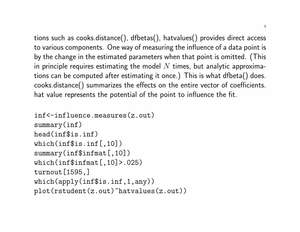
tions such as cooks.distance(), dfbetas(), hatvalues() provides direct accessto various components. One way of measuring the influence of a data point isby the change in the estimated parameters when that point is omitted. (Thisin principle requires estimating the model N times, but analytic approxima-tions can be computed after estimating it once.) This is what dfbeta() does.cooks.distance() summarizes the effects on the entire vector of coefficients.hat value represents the potential of the point to influence the fit.
inf<-influence.measures(z.out)
summary(inf)
head(inf$is.inf)
which(inf$is.inf[,10])
summary(inf$infmat[,10])
which(inf$infmat[,10]>.025)
turnout[1595,]
which(apply(inf$is.inf,1,any))
plot(rstudent(z.out)~hatvalues(z.out))

10
plot(1:nrow(turnout),cooks.distance(z.out))
summary(dfbeta(z.out))
plot(density(residuals(z.out)))
See Faraway 6.4 for more details.
2) Scalar measures of goodness of fit
Single number summary of fit, in the spirit of R2, or adjusted R2. Variousmeasures proposed, none having the clear interpretation of the linear modelR2, and no clear evidence of which ones are superior to others.
Information measures:
AIC = −2 ln L̂ + 2P
AIC is part of summary() output. −2 ln L̂ is the deviance of the model(deviance()), measuring how far the fit is from the best possible (for which

11
−2 ln L̂ = 0). So AIC is goodness of fit with penalty for model complexity(as reflected in P , number of parameters.) AIC the smaller the better.
BIC (Bayesian information criterion) is similar in spirit:
BIC = −2 ln L̂ + P lnN
Can show that 2 ln[Pr(D|M2)Pr(D|M1)
] ≈ BIC1 − BIC2 where the Bayes factor,Pr(D|M2)Pr(D|M1)
is the posterior odds of the models, if we have no prior preference
for one model against another. BIC smaller the better.
3) Goodness of fit should not be the criterion, at least not the only criterion,for evaluating models. Out of sample performance is what really matters.
A model could overfit and miss the underlying structure.

12
The possibility of over-fitting increases with model complexity. Generally,fitting gets better and better as the complexity increases, but out of sampleperformance worsens after certain point. [draw figure]
Make it a standard practice to reserve some of your data for out of sampleevaluation.
Dividing data into in-sample/out-of-sample is a special case of “cross vali-dation”, which involves dividing the data into k parts, each time leave onepart out in estimation and evaluate the model on the observations left out,then average the results over the k passes. the extreme form is “leave oneout”. Computationally intensive.
4) ROC curve:
If misclassifying a 1 is C times more costly than a 0 (e.g., war/peace), thendecision theory says predict Y = 1 if π̂ > 1/(1 +C). When C = 1, the cut
13
point is the usual .5.
If unsure what value of C to use, could draw the ROC curve, which plots %of 0’s correctly predicted against the % of 1’s correctly predicted, resultingfrom all sorts of cut point values in [0, 1] (reflecting all sorts of C values.) Abetter model has a larger area under the ROC curve. Ideally dominates theother model everywhere. (demo(roc) in Zelig; rocr package)
5) Calibration: Sort estimated probabilities into bins, say [0, 0.1), [0.1,0.2),... compute the mean predicted Pr in each bin, and the fraction of 1’s actuallyobserved in the corresponding observations. Plot the pairs. Systematicdeviation from the 45 degree line indicates problem.

14
2. Ordinal data: Ordered Logit and Probit
Start with the model for the latent Y ∗: Y ∗ = xβ + ε
Suppose the observed Y can take J ordered values, and suppose the obser-vation mechanism is
Pr(Y = j) = Pr(τj−1 ≤ Y ∗ < τj), j = 1, 2, . . . , J ; τ0 = −∞, andτJ =∞
Define Yij = 1 if Yi = j, 0 otherwise, then the likelihood function is:
P (Y ) =
n∏i=1
[
J∏j=1
Pr(Yij = 1)yij ] (1)
where
Pr(Yij = 1) = Pr(Yi = j) = Pr(τj−1 ≤ Y ∗i < τj)
= Pr(τj−1 ≤ xiβ + εi < τj)

15
= Pr(τj−1 − xiβ ≤ εi < τj − xiβ)
Assuming εi follows normal distribution, this becomes:
Pr(Yij = 1) = Φ(τj − xiβ)− Φ(τj−1 − xiβ) (2)
which is the Ordered Probit model. Ordered logit results from assumingthe logistic distribution for the errors. Interpretation is done using theseprobabilities (which sum to 1, of course). In general, the sign of the marginaleffects is unambiguous only for the smallest and the largest Y values!
Inserting this into (1), we have the likelihood function as a function of thedata (yij, xi) and the parameters (β, plus the J − 2 τ ’s—normalization getsrid of another τ ). MLE for the parameters are obtained by maximizing the(log) likelihood.
Zelig :
z.out <- zelig(as.factor(Y) ~ X1 + X2, model = ‘‘oprobit’’,

16
data = mydata)
(if Y is discrete integer with values reflecting the right order; otherwise firstcreate an ordered factor, see Zelig manual on ordered probit for an example.)
Interpretation can be similarly done as for binary probabilities (fitted values,first difference, marginal effect plot, etc.)
* demo(ologit)
Parallel regression assumption: Consider carefully the data observation mech-anism assumed in the ordered probit/logit models: there is one underlyingy∗ whose values give rise to the observed (ordered) categorical values ony. This assumption implies, in addition to the order probit/logit proba-bility expression, also expressions for a group of cumulative probabilities:pr(Y <= j), j = 1, 2, . . . , J − 1, which are given by:
Pr(Y <= j) = Pr(Y ∗ < τj) = Pr(xβ+ ε < τj) = Pr(ε < τj−xβ) (3)

17
which means that if you run a set of binary logit/probit models for Zj =(Y <= j), the β parameters in all of them should be identical, with onlythe constants differing from one another.
(see propodds() in library VGAM for model fitting and testing the assump-tion.)
When parallel regression assumption does not hold, consider models for un-ordered data. (Below.)

18
3. Multinomial Choice Models: Multinomial Logit and Pro-bit
Example: Vote choice with more than two candidates.
There are I decision makers, each individual i choosing among Ji (for no-tational simplicity, J hereafter) alternatives. Utility of alternative j to i isuij = vij + εij, where vij is a deterministic component, and εij is an un-observed, stochastic disturbance. vij is usually specified as a linear functionof observed independent variables, xiβj (multinomial logit), or wijγ (condi-tional logit or McFadden’s choice model), or xiβj +wijγ (mixed). mlogit inzelig estimates the multinomial logit model. for the other two with alterna-tive specific covariates, stata command asclogit is handy.
Under stochastic utility maximization, i chooses j if and only if uij > uikfor all k 6= j. So the probability of i choosing j is:
pij = Pr{uij > uik ∀k 6= j}

19
= Pr{vij + εij > vik + εik ∀k 6= j}= Pr{εik < vij + εij − vik ∀k 6= j}
=
∫ +∞
−∞
∫ vij+εij−vi1
−∞. . .
∫ vij+εij−viJ
−∞f (εi1, . . . , εiJ)dεiJ . . . dεi1dεij(4)
where f (εi1, . . . , εiJ) is the joint density of the ε′ijs. Let F (εi1, . . . , εiJ) bethe cumulative distribution function of the disturbances. Equation 4 can beequivalently expressed as:
pij =
∫ +∞
−∞Fj(vij + εij − vi1, . . . , εij, . . . , vij + εij − viJ)dεij (5)
where Fj is the partial derivative of F with respect to its jth argument.
From (4) or (5) a particular choice model is obtained by specifying the jointdistribution of the disturbances.
Criteria for choosing f (.) include functional flexibility (allow general patternsof heterogeneity and interdependence of the disturbances) and computational

20
ease.
The Multinomial Probit model is obtained by assuming that εij’s followa multivariate normal distribution. This allows relatively general covariancestructure. However, the multivariate normal cumulative distribution functionF (.) (and its partial derivatives) has no closed form solutions, so for probitchoice probabilities expression (5) is a simplification of (4) only in notation.The computation involves dealing with multiple integrals (through numericalmethods or by simulation). Costly when the choice set contains more thana few alternatives.
The Multinomial Logit model results from assuming that εij have i.i.d. ex-
treme value distribution: F (εij) = e−e−εij
. Unlike the normal distributionfunction, the cumulative distribution function F (.) here has a closed form,

21
and logit choice probabilities pij can be derived from equation (5) as:
pij = evij/
J∑k=1
evik, j = 1, 2, . . . , J (6)
with∑
j pij = 1.
Likelihood function formed similar to ordered probit (1). Note that onlyJ−1 sets of parameters can be estimated (any alternative k can serve as the“base” category. If none of the variables matter for a particular comparison,the two categories can be combined.)
The mlogit probabilities have intuitive interpretations: the higher the relativeutility provided by an alternative, the higher the probability of that alternativebeing chosen. mlogit is a generalization of binary logit, of course. (show it.)mprobit similarly generalizes binary probit.
Zelig :

22
z.out <- zelig(as.factor(Y) ~ X1 + X2, model = "mlogit",
data = mydata)
“setx()” and “sim()” used the standard way. Quantities of interest evolvearound the J probabilities (first differences, risk ratios, etc.) If J = 3, coulddo ternary plot. (See Zelig manual, example for mlogit. Mexican 3-partyelection. Substantive question: if voters had thought the ruling PRI partywas weakening, who’d have won??)
Run “demo(mlogit)”.
Generalizations. The mlogit model is computationally simple. However, εij’sare assumed to be independent and identically distributed. → Homoscedas-tic errors. Restrictions also include the IIA (independence from irrelevantalternatives) property: the ratio of the choice probabilities of any two alter-natives not affected by the presence of other alternatives (show.) IIA notplausible when some alternatives are close substitutes.

23
The Nested logit model generalizes the mlogit and relaxes the IIA restriction:“similar” alternatives grouped into subsets, error terms within the subsetscan be correlated. The GEV (generalized extreme value) model is a furthergeneralization, the choice probabilities taking the form:
pij = evijGj(evi1, . . . , eviJ)/G(evi1, . . . , eviJ) (7)
where G(Y1, . . . , YJ) is a non-negative generating function (satisfying a setof technical conditions that ensure the joint distribution and the resultingmarginal distributions are well defined), and Gj is the partial derivative of Gwith respect to its jth argument.
The standard mlogit model results when
G(Y1, . . . , YJ) =∑J
k=1 Yk. (verify)
24
The nested logit model results from G taking the form:
G(Y1, . . . , YJ) =
K∑k=1
(∑i∈Ik
Y1/σki )σk (8)
where Ik ⊂ {1, . . . , J} , ∪Kk=1Ik = {1, . . . , J}, and 0 < σk ≤ 1. Thus theJ alternatives are grouped into K subsets. The parameter σk is interpretedas an index of the similarities of the alternatives within subset Ik. Whenσk ≡ 1, the nested logit model reduces to the mlogit model. (stata: nlogit.)
However, the entire GEV class of models still imposes homoscedasticity. Thegeneralized GEV class (Zeng 2000) allows for heteroscedasticity, with the het-eroscedastic logit/mlogit model being a special case. When heteroscedastic-ity is across individuals only (not alternatives), the choice probabilities retaina simple/intuitive form:
pij = evijθi/
J∑k=1
evikθi (9)
25
where θi’s are inversely related to the standard error of the error terms.Intuitively, meaning more weight is given to individuals whose utility functionshave smaller error variances. With heteroscedasticity across alternatives also,the model is:
pij =
∫ ∞
−∞θije
−εθij exp{−J∑k=1
e−(vij+ε−vik)θik}dε (10)
This involves only one dimensional integration, regardless of the numberof alternatives J (unlike mprobit). θi or θij can be specified as functionsof covariates with unknown parameters to be estimated along with otherparameters in the model, and in the θij = θi case the model can be estimatedwith programs for standard models with simple transformation of variables.Alternatively, θ’s can be given their own distributions, resulting in a class ofrandom parameter logit models.