PRR Is Not Enough

Kannan Srinivasan, Maria A. Kazandjieva, Mayank Jain, Philip LevisComputer Systems Lab

Stanford UniversityStanford, CA 94131

{srikank,mariakaz,mayjain}@stanford.edu, pal@cs.stanford.edu.

AbstractWe study the effects of wireless channel burstiness on TCP.We measure TCP throughput over single-hop link traces fromMIT’s 802.11b Roofnet and Intel Berkeley’s 802.15.4 Mi-rage testbeds. We observe that links with the same packetreception ratio (PRR) have throughput variations of up to320%. We find that differences in throughput are accom-panied by differences in link burstiness. Using the Gilbert-Elliott model, we compute the parameter µ as a measure ofburstiness. We show that for sufficiently large data traces, asimple second-order fit over both PRR and µ lowers the es-timation error of TCP throughput by 50%. The estimationerror reduces by 60%-99% for a more general fit over PRRand µ. We find that while µ has good deductive quality, thecorresponding Gilbert-Elliott model is not accurate for simu-lation: TCP throughput values from empirical links and theircorresponding simulated links based on the Gilbert-Elliottmodel can differ by up to 80%. These results help developa better understanding of the underlying causes for the widevariations seen wireless network performance.

1. Introduction

This paper is a measurement study of the dynamics andbehavior of wireless links. It strives to broaden the insightinto real-world systems as well as take a step toward bridgingthe gap between empirical observations and simulation.

Wireless protocol design is notoriously difficult. This isespecially true with open-spectrum technologies, such as802.11b, 802.11g, 802.11n, Bluetooth and 802.15.4, all ofwhich share a 2.4GHz band with cordless phones, microwaves,and other consumer devices. Being in an open band makesthese technologies inexpensive and therefore ubiquitious. How-ever, in practice, this means that their RF environments tendto be complex, interference-heavy, and hard to tackle withclean analytical approaches or simulations.

Researchers have addressed this challenge by deploying,testing, and evaluating protocols on indoor and outdoor meshtestbeds [27, 4, 8, 9, 10, 17, 19, 20, 29]. Deploymentsdemonstrate that a protocol can work in practice, but their

results are difficult to generalize. Two separate testbeds canproduce completely different results. To explain this varia-tion, deployment studies typically report high-level networkproperties, such as a connectivity graph, reception ratios, av-erage hop count, and average degree.

These properties seek to succinctly describe the dynam-ics of a very complex system. While useful for highly gen-eral observations – e.g., lossier networks will have lowerthroughput – they are not sufficient for explaining fine-grainedperformance results. Deployments can demonstrate whethera protocol works, but generalizing to predicting performanceon another wireless mesh remains out of reach.

If these metrics are insufficient for explaining networkperformance, then what else should we measure? A com-plete answer to this question would enable a rigorous analyt-ical understanding of wireless protocols that matches experi-mental results. This paper is a first step towards developing asystematic methodology for characterizing wireless deploy-ments. It provides an insight on a new measurement, channelburstiness, and its effect on TCP throughput.

This paper examines the most simple and basic commu-nication case: a single pair of communicating nodes. Usingpacket traces from 802.11b and 802.15.4 testbeds, we findthat single-hop TCP throughput for two links with the samepacket reception ratio can vary by as much as 320%. There-fore, packet reception ratio measurements are not enough topredict TCP throughput. Looking at what differs betweensuch links, we see that links with the same reception ratio lostpackets in very different ways. Links with higher throughputhave bursts of losses, while links with lower throughput haverandom, independent losses.

If loss burstiness can affect protocol performance, we needa way to measure it. We draw on several proposals from liter-ature and choose µ as a metric of burstiness. µ is computedfrom the Gilbert-Elliott channel model and measures aver-age link burstiness. We find that µ, combined with the PRR,can accurately predict TCP throughput for links with PRRbetween 20% and 60%. Section 7 shows that adding µ intoconsideration reduces the error of estimated TCP throughputby 50%-99% as opposed to using only the reception ratio of

1

the link. Therefore, reporting a link’s µ can give an enhancedunderstanding of a wireless network.

The strong correlation that µ has with the behavior ofTCP raises the question of whether µ describes the actualunderlying dynamics in wireless links. If the Gilbert-Elliottmodel accurately captures what causes these performancevariations, then it can be used in simulators to improve theirresults. To test this hypothesis, we derive Gilbert-Elliottmodels from measured µ values and link reception ratios.Comparing the TCP throughput of the real links with sim-ulated links shows that they can differ by as much as 80%.While µ describes some link property that is correlated withTCP performance, links do not follow a Gilbert-Elliott model.

This paper’s three research contributions are scientific anddescriptive. First, we observe that there are TCP throughputvariations that PRR cannot fully account for. Second, wefind that burstiness can explain much of these variations andreduce throughput estimation error by 50%-99%. Third, wefind that while µ has significant deductive value in explain-ing a network, the Gilbert-Elliott model from which it comesdoes not accurately describe a link, and that more informa-tion, such as burst lengths, is necessary for simulation.

The rest of the paper is structured as follows. Section 2describes related work on burstiness, TCP, and modeling wire-less links. Section 3 describes the testbeds and data traces,as well as our TCP NewReno implementation. Section 4shows that PRR is not enough to understand TCP’s perfor-mance. Section 5 presents the Gilbert-Elliott model and amethod for quantifying burstiness. Section 6 examines howµ correlates with TCP performance in 802.15.4 and 802.11bnetworks. Section 8 shows that the time over which we ob-serve a link needs to be long enough for µ to converge to astable value. Section 9 explores whether the TCP results im-ply simulators can use a Gilbert-Elliott model to good effect.Finally, Section 10 concludes and discusses future work.

2. Related Work

Although TCP was designed for wired networks, it is widelyused in the wireless domain for easy interoperability betweenthe wired backbone and the last mile 802.11 and cellularnetworks. In addition, TCP/IP over 802.15.4 has recentlygained momentum within the embedded network industrybecause to its interoperability and openness, with the IETFforming working groups [25, 3] to support the effort.

One of the main reasons for TCP’s poor performance overwireless is its rate adaptation for packet losses: TCP assumesthat all losses are due to congestion while in wireless net-works losses can be because of channel errors [7]. This leadsto degraded performance of TCP over wireless.

In the past, TCP performance analysis took in to accountonly the average loss rate [22, 21]. Lakshman et. al. [22] an-alyze TCP/IP performance in networks where the bandwidth-delay product is higher than the buffering, assuming randompacket losses. Kumar et. al. [21] also assume random packet

losses but analyze the effects of fast retransmit, fast recoveryand coarse timeouts of different types of TCP.

Ignoring correlation of reception in links can lead to in-accurate results [32, 31, 6]. Correlation of reception in wire-less links is typically modeled as a simple two state markovchain [13, 28, 32], the Gilbert-Elliott model being the mostpopular. Altman et. al. [6] model packet loss as a two stateMarkov process and analyze moments of TCP throughput.Yet, for simplicity, protocol designs typically assume links tohave time independent reception [1, 2] with the packet recep-tion ratio being the only modeling parameter. For instance,the immediate retransmissions in many MAC protocols as-sume that a packet failure and the immediate retry attempthave independent fates.

In practice, many wireless links are not as simple as a 2-state markov model [18, 20]. While it is an easy model toanalyze, it is not accurate for all real links.

Jiao et. al. have shown that the two state markov modelis inadequate to model link burstiness and that wireless linksmay be better modeled using inhomogenous markov chainsin which the transition probabilities are not constants[18].Kopke et. al. use real data traces and show that simplemodels like the Gilbert-Elliott model do not simulate the reallinks well by comparing the run-length distributions of reallinks and the links generated by simple models[20]. Theyshow that chaotic maps can yield far better simulation mod-els. There is also work that shows simple models such asthe 2-state model can yield inaccurate predictions of higherlayer protocol performance [18, 12].

In this paper, we do not propose a new way to quantifyburstiness nor do we propose a new model to make simula-tions better. We look deeply at a simple parameter, µ fromthe Gilbert-Elliott model and see how correlated it is withTCP’s performance. Unlike most work in the literature, westart from testbed data traces to study the TCP performance.We do not use simulations that use abstracted statistical mod-els for the wireless channel but rather feed the real worldtraces as input to the simulator.

3. Methodology

This section describes the experimental methodologies ofthis paper, including the data sets, their high-level properties,and the simulation setup used to measure TCP throughput.

3.1 TCP ImplementationTo measure TCP throughput, we use a nesC implemen-

tation of the NewReno TCP stack [5, 11, 30, 16] on top ofTOSSIM [23]. TOSSIM simulates an environment of sen-sor nodes running TinyOS [15]. TinyOS is an event-drivenoperating system, specifically designed for network protocolimplementations on embedded systems. nesC is an extensionof the C language for programming in TinyOS.

To evaluate the performance of TCP, we feed datatraces ofpacket receptions and losses into TOSSIM. TCP signals the

2

0.0 0.2 0.4 0.6 0.8 1.0Packet Reception Ratio

0%

20%

40%

60%

80%

100%%

Lin

ks

(a) Mirage - Channel 26

0.0 0.2 0.4 0.6 0.8 1.0Packet Reception Ratio

0%

20%

40%

60%

80%

100%

% L

inks

(b) Mirage - Channel 16

0.0 0.2 0.4 0.6 0.8 1.0Packet Reception Ratio

0%

20%

40%

60%

80%

100%

% L

inks

(c) Roofnet - 11Mbps

Figure 1: Cumulative distribution of packet reception ratios in the three data sets. Most links are either poor or excellentbut there are about 20% to 30% which fall in the intermediate PRR range.

simulator for a packet transmission; the success or failure ofthat packet is determined by the datatrace entry at the corre-sponding time. We are only interested in single-hop trans-missions in order to understand a link’s most basic behavior;we calculate the TCP throughput in packets per second.

While the RFC documents detail most TCP specifications,TCP sender and receiver timeout values are not explicitlystated. The timeout values in typical implementations aretuned for a multi-hop wired network with long Round-triptimes. These values are not applicable to the single-hop wire-less links studied in this paper. Here we briefly explain ourchoice of values for these variables.

On the sender’s side, the retransmission timeout is subjectto an upper and a lower bound. Ideally, the timeout mustbe greater than the time it takes to transmit one window ofdata, so not all packets in flight are retransmitted. In ourTCP implementation, the maximum congestion window is130 packets, but this number is rarely reached. For datatraceswith 10ms interpacket interval it would take 1.3 seconds tosend a window of data, but the size of the window is usuallymuch smaller. Based on this, we can choose the lower boundof the retransmission timeout as 1 second, together with 60seconds for the upper bound.

The ACK timeout on the receiver’s side governs how longto wait for a packet before sending an acknowledgement.The timeout should be significantly lower than the sender’sretransmission timeout, so the sender gets up-to-date infor-mation when there are a lot of losses. We choose an ACKtimeout of 300ms for the data traces with 10ms interpacketinterval. Since both timeouts depend on the interval betweenpacket transmissions, in the following subsection we men-tion how TCP timeout values vary between data sets.

3.2 DatasetsWe use datasets from two testbeds, namely Mirage and

Roofnet.

3.2.1 802.15.4 Mirage Data802.15.4 is an IEEE PHY-MAC standard for low power,

low data rate networks. We measure 802.15.4 using the IntelMirage testbed [17] - a set of indoor ceiling nodes.

10% 90%0% 100%

Intermediate VeryGood

VeryPoor

NoLink

Perfect

Packet Reception Rate

Poor Good

60%20%

Figure 2: Terminology used to describe links based onPRR. Very poor links have a PRR < 10%, poor arebetween 10% and 20%, intermediate links are between20% and 60%, and good and very good links are > 60%.A PRR of 100% is a perfect link.

To collect the Mirage datatraces, each node transmits broad-cast packets every 10ms for a 1000-second duration, giving atotal of 100,000 packets. All other nodes listen and a centralserver logs packet receptions. We collected data for two dif-ferent 802.15.4 channels, channel 16 and channel 26. Chan-nel 16 overlaps with the 802.11b transmission band and thusis subject to external interference from Intel’s WiFi network,while channel 26 has very little interference.

3.2.2 802.11b Roofnet DataIn addition to Mirage, we used 802.11b datatraces from

MIT’s Roofnet study [4]. The traces were collected from anoutdoor, wireless mesh network, operating at 11Mbps and1Mbps. Similarly to Mirage, every node take its turn tobroadcast packets.

In the 11Mbps case, packets were sent as fast as possiblefor 60 seconds; we subsample this data to produce 20000-packet traces with an inter-packet interval of 2ms and totalrunning time of 40 seconds. Since packet transmissions takemuch longer in the 1Mbps experiments, the inter-packet in-terval is 20ms, and the the total number of packets - 3000.Section 8 shows that a trace length of 3000 is not enough forvalues of µ to converge. Therefore, in this paper we onlyuse the 11Mbps Roofnet data traces. Since the Roofnet andMirage data differ in the number of packets sent per second,100 versus 500, we scale the TCP timeout parameters appro-priately. This reduces the retransmission timeout upper andlower bounds to 200ms and 12 seconds respectively, and theACK timeout to 60ms.

3

0.0 0.2 0.4 0.6 0.8 1.0Packet Reception Ratio

0

20

40

60

80

100Pack

ets

per

Seco

nd

70% difference

250% difference

(a) Mirage Channel 26

0.0 0.2 0.4 0.6 0.8 1.0Packet Reception Ratio

0

20

40

60

80

100

Pack

ets

per

Seco

nd

up to 320% difference

(b) Mirage Channel 16

0.0 0.2 0.4 0.6 0.8 1.0Packet Reception Ratio

0

100

200

300

400

500

Pack

ets

per

Seco

nd

200% difference

(c) Roofnet

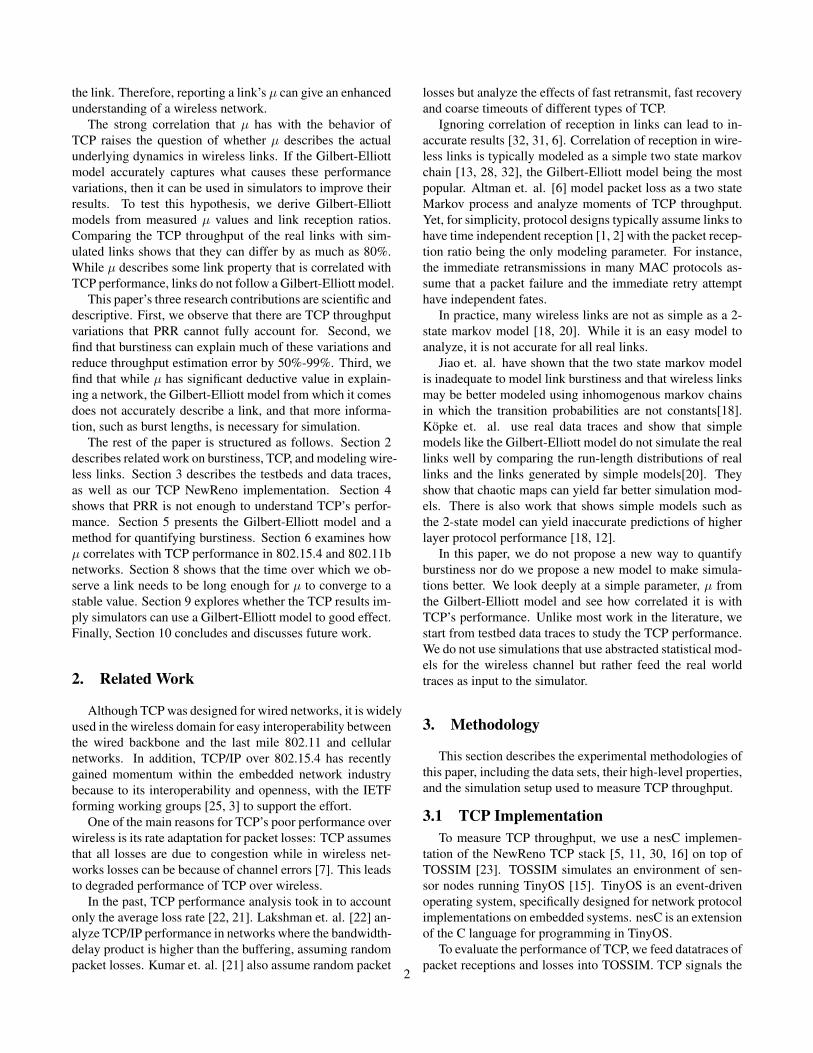
Figure 3: Single-hop TCP throughput measurements for 802.11b and 802.15.4 datatraces. Within a given receptionratio, throughput varies by 20 to 320%.

3.3 Link Packet Reception RatiosFigure 1 shows the cumulative distribution of reception

ratios for the three datasets. A majority of the links haveeither a very high or very low PRR. The first, rarely leavespace for improvement, while the latter might be impossibleto improve.

Between 25% and 40% of the links have a variety of PRRsbetween 0.1 and 0.9. In addition, Sections 4 and 6 show thatlinks with PRR between 0.2 and 0.6 are of significant interestwhen analyzing TCP throughput.

Figure 2 defines the terminology used in the rest of thispaper to describe the reception ratios of wireless links. Weuse the terms very poor, poor, intermediate, good, very good,or perfect. We begin by examining all links that are poor,intermediate, and good, and then concentrate only on the in-termediate links with PRR between 0.2 and 0.6. In the twoMirage datasets there are about 50 single-hop intermediatelinks, while in the Roofnet dataset there are over 120 inter-mediate data traces.

4. PRR Is Not Enough

The performance of multihop flows in wireless meshestypically falls well below what link-level bitrates would sug-gest. For example, simple unicast routing protocols, suchas Srcr [8], exhibit approximately ten-fold reduction in TCPthroughput between single-hop paths and paths longer than4 hops. Approaches that take advantage of the broadcast na-ture of a wireless channel, such as ExOR’s opportunistic re-ceptions [9], or COPE and MORE’s network coding [19, 10]see significant (35-1000%) throughput gains on some paths,but they still exhibit a ten-fold spectrum in performance.

The poor quality of wireless links is one possible expla-nation for this disparity. Another explanation is the choicesmade by routing protocols. It is important to first understandhow TCP performance varies for single-hop paths, before in-vestigating performance over multi-hop paths.

Figure 3 shows results for the three datasets described inSection 3. The TCP throughput is plotted against the link’sPRR. As expected, PRR captures the general trend of in-

creased throughput for higher reception ratio links. However,there are a number of cases in which two or more links havevery similar PRR, yet different TCP throughput. The major-ity of throughput discrepancies happen in the intermediatereception ratio range, 20% to about 60%. For example, in theMirage channel 26 data, a link with a PRR of 0.33 achievesTCP throughput of barely 2 packets per second, while an-other link with a PRR of 0.35 is at over 7 packets per second.

These two links will appear the same based on PRR alone,yet have a difference of over 250% in TCP performance.Similar observations are true for Channel 16 – for examplethree links with a PRR of 0.37 have TCP throughputs of 3, 8,and 14 packets per second respectively, resulting in a differ-ence of up to 320%. In Roofnet, links with equal receptionratio can experience throughput variations of over 200%.

Therefore, even though PRR gives a coarse-grained un-derstanding of what the expected throughput of a link is, it isnot enough. However, in these experiments, PRR is the onlyvariable in the classical formula for TCP throughput, as bothRTT and MTU are fixed. The formula for predicting TCPthroughput is:

Throughput = 1.3 · MTU

RTT ·√Loss

There have been many modifications proposed to this equa-tion to account for other TCP parameters such as timeoutsand the number of packets acknowleged by a single ACK [24].One drawback that Padhye et al. [26] have addressed is thatthe equation does not work well for channels with more than2% losses.

All suggested modifications to the TCP throughput for-mula consider a wired multi-hop packet switched network.On the other hand, our experiments look at single-hop wire-less TCP connections where packets are sent at regular in-tervals, and flight size and TCP performance are not RTT-constrained. In addition, links in the Mirage and Roofnetdatasets exhibit losses much greater than 2%, and it is notclear how well the classic throughput equation will handlelinks with such low PRRs.

Furthermore, current TCP equations assume uniformlyspaced losses. This is a worst case scenario since each loss

4

5 10 15 20Length of Burst

0%

20%

40%

60%

80%

100%B

urs

tsLink 1

Link 2

Link 1

Link 2

Figure 4: CDF of loss burst length for two links with thesame PRR, in the Mirage testbed. Since one link has iso-lated losses more than 95% of the time, its TCP through-put is much lower than the other link.

maximally decreases the congestion window size. Losses onwireless links are often correlated, making links bursty. It isthe temporal distribution of losses, in addition to their num-ber, that affects TCP performance.

Figure 4 shows the cumulative distribution of loss burstlengths for the two links in the Mirage channel 26 dataset,shown in Figure 3, that have a TCP throughput differenceof 250%. In order to focus on shorter runs of losses, weonly show the x-axis up to 40 packets, capturing 99% of thebursts. For one link, 55% of all losses happen in isolation –the lost packet was preceded and followed by one or moresuccesses. For the second link, that value is over 95%. In-tuitively, the latter link has more independent losses, and asexpected [14], is the link with lower throughput. These ob-servations suggest that channel burstiness is a useful param-eter that can give an insight in to protocol performance.

If such large differences in TCP throughput are possibleover single-hop paths, then it is no surprise that multi-pathmesh networks can exhibit significant variations in their per-formance. Aguayo et al.’s study of Roofnet [4] found thatmany of its links had bursty behavior, and studies of 802.15.4have found similar behavior [29].

Therefore, in such networks, PRR is not enough to accu-rately characterize links. Instead, we need to expand the setof properties we measure and report on wireless links – ourexperimental lexicon. We need to find a suitable parameterfor reporting burstiness in addition to other measurements.First, we must find the best way to quantify burstiness andthen understand how this new parameter alters TCP through-put predictions.

5. Quantifying Burstiness

This section introduces the Gilbert-Elliott channel modelthat has been widely used in the RF community. It is amethod for modeling channel memory, which has a directimplication on its burstiness. Although most literature treats

Bad Good

b

g

1-b1-g

µ = 1 - b - g

Figure 5: The Gilbert-Elliott model of a wireless link.

the Gilbert-Elliott model as a bit model, we use it as a packetmodel, i.e. we model bursts of packet errors and successesrather bursts of bit errors and successes.

5.1 Defining BurstinessIn simple terms, link burstiness is the property of hav-

ing temporally correlated losses and successes on a wirelesslink. A good first step towards defining what a bursty linklooks like is to define what a bursty link does not look like.A link is not bursty when its packet successes and failuresare not temporally correlated, i.e. the success and failure ofeach packet delivery is independent of all previous and fu-ture packet transmissions. While such a link will have runsof successes and failures, the lengths of these runs will fol-low a geometric distribution.

A bursty link is one where there is a positive correlationbetween similar packet events. Given a reception ratio R, theprobability of receiving a second packet after one arrives suc-cessfully is greater than R, while the probability of receivinga second packet after one does not arrive successfully is lessthan R.

It is also possible for a link to be oscillatory. In an os-cillatory link, there is a negative correlation between similarpacket events. Links that quickly swing back and forth be-tween periods of good and bad reception can introduce thisbehavior. Receiving a packet makes it more likely that a pe-riod of bad reception is about to follow and not receiving apacket makes it more likely that a period of good receptionis about to occur.

5.2 Gilbert-Elliott ModelThe Gilbert-Elliott model of a wireless link, shown in Fig-

ure 5 is a two-state Markov process. The states of the processcorrespond to the link being in a “good” state (zero probabil-ity of packet errors) or the link being in a “bad” state (non-zero probabiity of packet errors). The Gilbert-Elliott modelhas three parameters, g, the probability of transitioning tothe good state from the bad state; b, the probability of tran-sitioning to the bad state from the good state; and h, the lossrate in the bad state. The model assumes the good state hasno errors and many analytical formulations assume, for sim-plicity, that the bad state loses all packets (h = 100%). Therest of this paper assumes h equal to 100%.

The memory of the Gilbert-Elliott model is given by aparameter µ. A model’s µ, defined as 1− g − b, has a directimplication on the burstiness of the channel. If µ is zero, then

5

b = (1−g) and g = (1−b). Put another way, the probabilityof transitioning to the good or bad state is independent ofwhat state the model is in. As µ approaches 1, the probabilityof transitioning away from states approaches zero, causingthe links to be very bursty. As µ approaches -1, the statesare more likely to transition than to stay the same, causingoscillatory behavior.

In the case where h = 100%, the parameters g and b arethe probability of a successful packet following a packet fail-ure and the probability of a packet failure following a suc-cessful packet. Encoding packet delivery as a binary string,g = |01|

|01|+|00| and b = |10||10|+|11| .

5.3 Calculating µ For Empirical Channelsµ can be calculated for empirical channels from the data

traces outlined in Section 3. As mentioned earlier, we usea simplified Gilbert-Elliott model where each failure corre-sponds to the bad state and each success corresponds to thegood state. Looking at empirical data traces can give all statetransitions for this model by labeling each failure as bad stateand success as good state. States can then be encoded by bi-nary numbers with 0 denoting bad state and 1 denoting goodstate. For example, a good to bad state transition will corre-spond to the occurance of a “10” in the bit stream and a badto good transition to the occurance of a “01”. Thus, usingthe packet delivery data encoded as a binary string and theequations for g and b from above, we can find g and b andalso µ = 1− g − b.

6. TCP Performance

This section investigates the effect of burstiness on TCPperformance for different testbeds. The TCP simulator (ex-plained in Section 3) is run on packet traces obtained for thevarious testbeds, Mirage on Channels 26 and 16 and Roofnet,to evaluate TCP performance in packets per second.

In order to measure the effect of burstiness for differentlinks, we synthesize an independent link with the same PRRas the empirical link under consideration. For an indepen-dent link, each packet has a probability of success equal tothe PRR of the link,regardless of the fate of previous or fu-ture packets. Thus, to generate data for the independent link,we generate a bit pattern where each bit is 1 (meaning suc-cess) with a probability equal to PRR and 0 otherwise. Thelength of the synthesized trace is made equal to the lengthof the empirical trace for each link. For comparison of TCPthroughput, the TCP simulator is then run on the data tracesfor the empirical link and the corresponding synthesized in-dependent link and difference in throughput for the burstylink is noted.

6.1 Initial ObservationsFigure 6 shows the plot of TCP throughput difference for

the Mirage channel 26 trace for all links with PRRs between10% and 90%. TCP throughput difference for various links

0.0 0.2 0.4 0.6 0.8Mu

-200%

-100%

0%

100%

200%

300%

400%

500%

600%

700%

Thro

ughput

Diffe

rence

0.2

0.3

0.4

0.5

0.6

0.7

0.8

Figure 6: TCP throughput difference compared to a syn-thesized independent link for links with different µ andPRRs for Channel 26 Mirage testbed.

0.0 0.2 0.4 0.6 0.8Mu

-200%

-100%

0%

100%

200%

300%

400%

500%

600%

700%

Thro

ughput

Diffe

rence

0.1

0.2

0.3

0.4

0.5

0.6

0.7

0.8

Figure 7: TCP throughput difference compared to a syn-thesized independent link for links with different µ andPRRs for the Roofnet testbed running at 11mbps.

is measured in comparison to the synthesized independentlinks for the same PRR and plotted versus the µ values forthese links. The PRR levels are coded in shades of gray.Figure 7 shows the same plot for Roofnet data. The generaltrend of increasing throughput with increasing µ is visible inboth plots, but there are a lot of outliers.

The outliers tend to occur at high PRRs (> 60%), wherethe difference is less than expected and very low PRRs (<20%), where the difference is greater than expected. A betterunderstanding of behavior of the Gilbert-Elliott model forhigh and low PRRs can explain the existance of outliers forthese PRR values.

6.2 Gilbert-Elliott Model Behavior On ExtremePRRs

The increase in TCP throughput as an effect of burstinessis the result of an increase in the number and the length ofruns of successes in a link trace compared to the independentlink with the same PRR. As an approximation, we can com-pare the difference by looking at the probability of 2 consec-utive successes in a trace for the two cases. To calculate thisprobability for the Gilbert-Elliott model explained in Section5, we need to calculate the values of parameters g and b and

6

-0.1 0.0 0.1 0.2 0.3 0.4 0.5 0.6 0.7 0.8Mu

-100%

-50%

0%

50%

100%

150%

200%

250%

300%

350%Thro

ughput

Diffe

rence

0.24

0.28

0.32

0.36

0.40

0.44

0.48

0.52

0.56

Figure 8: TCP throughput difference compared to a syn-thesized independent link for links with different µ andintermediate links for channel 26 Mirage testbed.

the steady state probabilities of being in the good and the badstates in terms of PRR and µ.

We call the steady state probabilities of being in the goodand the bad statesG andB respectively. Then, G = PRR andB = 1 - PRR. Further, in steady state, G ∗ b = B ∗ g. Usingthese and µ = 1− b− g, we get b = (1− PRR) ∗ (1− µ)and g = PRR ∗ (1 − µ). The probability of 2 consecutivesuccesses is given by G ∗ (1− b).

For a PRR of 0.1 and µ of 0.6, the probability of 2 con-secutive successes is 0.06 for the bursty link and 0.01 for theindependent link. This represents a large percentage increasein the probability of getting a burst and correspondingly, alarge increase in the observed TCP throughput difference.

For a PRR of 0.9 and µ of 0.6, the probability of 2 con-secutive successes is 0.864 for the bursty link and 0.81 forthe independent link. This represents a very small percent-age increase in the probability of getting a burst and corre-spondingly, a small increase in the observed TCP throughputdifference. Therefore very high and very low PRR values donot adhere to the general trend observed for TCP throughputdifference.

6.3 Observations For Intermediate LinksFigure 8 shows the plot of TCP throughput difference

for intermediate links for channel 26 on the Mirage testbed.These links show a clear correlation between increasing through-put difference and increasing µ. Figure 9 shows the sameplot for Mirage channel 16. Figure 10 shows the TCP through-put difference with µ for the Roofnet traces. In all threetestbeds, an increase in µ has an accompanying increase inTCP throughput: this effect appears across different wirelesschannels in the 2.4Ghz band and across different data rates.

7. Data Fitting Analysis

Section 4 observed large variations of TCP throughput atintermediate PRR values. Section 6 showed that the varia-tions in TCP throughput can be attributed to link burstiness

-0.1 0.0 0.1 0.2 0.3 0.4Mu

-80%

-60%

-40%

-20%

0%

20%

40%

60%

80%

100%

Change in T

hro

ughput

0.24

0.28

0.32

0.36

0.40

0.44

0.48

0.52

0.56

Figure 9: TCP throughput difference compared to a syn-thesized independent link for links with different µ andintermediate links for channel 16 Mirage testbed.

-0.1 0.0 0.1 0.2 0.3 0.4 0.5 0.6 0.7 0.8Mu

-100%

0%

100%

200%

300%

400%

500%

Thro

ughput

Diffe

rence

0.24

0.28

0.32

0.36

0.40

0.44

0.48

0.52

0.56

Figure 10: TCP throughput difference compared to asynthesized independent link for links with different µand intermediate links for Roofnet testbed running at11mbps.

and the Gilbert-Elliott channel memory parameter µ can beused to quantify this burstiness.

To evaluate the effect of the calculated µ on TCP through-put, this section looks at the accuracy of estimation of TCPthroughput using only PRR and compares this with the accu-racy obtained by using both PRR and µ. TCP estimates arecalculated by finding the best fits based on the least L1 normof error1. L1 norm is used rather than Least Squares becauseit is more robust to outliers.

The TCP throughput expression in Section 4 shows thethroughput to be proportional to the inverse square root ofthe loss rate, i.e. ∝ 1√

1−PRR . As discussed before, this ex-pression may not be applicable to single hop links with highloss rates. Our experiments have also shown that a second or-der estimate provides a good fit for observed TCP throughputbased on PRR values. Comparing best fits for TCP through-put for linear fit, quadratic fit and fit with 1√

1−PRR shows the

1L1 norm of the error is the sum of the absolute values of error ateach data point

7

(a) Mirage - Channel 26 (b) Mirage - Channel 16 (c) Roofnet

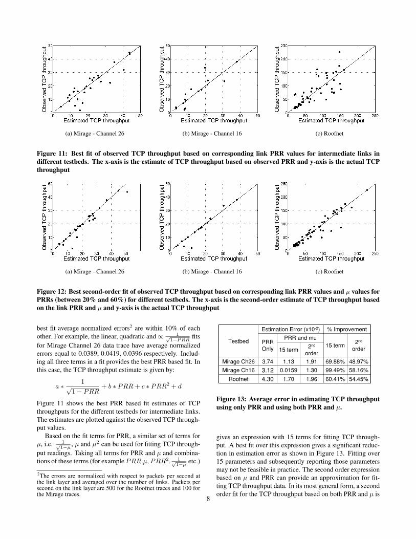
Figure 11: Best fit of observed TCP throughput based on corresponding link PRR values for intermediate links indifferent testbeds. The x-axis is the estimate of TCP throughput based on observed PRR and y-axis is the actual TCPthroughput

(a) Mirage - Channel 26 (b) Mirage - Channel 16 (c) Roofnet

Figure 12: Best second-order fit of observed TCP throughput based on corresponding link PRR values and µ values forPRRs (between 20% and 60%) for different testbeds. The x-axis is the second-order estimate of TCP throughput basedon the link PRR and µ and y-axis is the actual TCP throughput

best fit average normalized errors2 are within 10% of eachother. For example, the linear, quadratic and ∝ 1√

1−PRR fitsfor Mirage Channel 26 data trace have average normalizederrors equal to 0.0389, 0.0419, 0.0396 respectively. Includ-ing all three terms in a fit provides the best PRR based fit. Inthis case, the TCP throughput estimate is given by:

a ∗ 1√1− PRR

+ b ∗ PRR+ c ∗ PRR2 + d

Figure 11 shows the best PRR based fit estimates of TCPthroughputs for the different testbeds for intermediate links.The estimates are plotted against the observed TCP through-put values.

Based on the fit terms for PRR, a similar set of terms forµ, i.e. 1√

1−µ , µ and µ2 can be used for fitting TCP through-put readings. Taking all terms for PRR and µ and combina-tions of these terms (for example PRR.µ, PRR2. 1√

1−µ etc.)

2The errors are normalized with respect to packets per second atthe link layer and averaged over the number of links. Packets persecond on the link layer are 500 for the Roofnet traces and 100 forthe Mirage traces.

48.97%69.88%1.911.133.74Mirage Ch26

58.16%99.49%1.300.01593.12Mirage Ch16

2nd

order15 term

2nd

order15 term

PRR and muPRR Only

54.45%60.41%1.961.704.30Roofnet

% ImprovementEstimation Error (x10−2)

Testbed

Figure 13: Average error in estimating TCP throughputusing only PRR and using both PRR and µ.

gives an expression with 15 terms for fitting TCP through-put. A best fit over this expression gives a significant reduc-tion in estimation error as shown in Figure 13. Fitting over15 parameters and subsequently reporting those parametersmay not be feasible in practice. The second order expressionbased on µ and PRR can provide an approximation for fit-ting TCP throughput data. In its most general form, a secondorder fit for the TCP throughput based on both PRR and µ is

8

given by an equation of the form:

a ∗ PRR+ b ∗ PRR2 + c ∗ µ+ d ∗ µ2 + e ∗ PRR ∗ µ+ f

where a, b, c, d, e and f are constant coefficients. Figure 12shows the best PRR and µ based second order fit estimatesof TCP throughputs for the different testbeds and intermedi-ate PRRs. As can be seen from the figures, incorporating µfor estimating TCP throughput improves the fit considerablyeven with the second order approximate fit being used. Nu-merically, incorporating µ into the estimate reduces the L1norm of the error by more than 60% by using the 15 termexpression and by approximately 50% by using the secondorder fit expression. Figure 13 summarizes the results for theaverage error in estimation for different datasets using onlyPRR and both PRR and µ. The table shows results from bothusing the 15 term expression combining µ and PRR and thesecond order approximation. The percentage improvementshown is improvement of each fit over the PRR only fit. Theaverage errors are normalized based on the link level packetsper second and averaged over the number of links.

An observation in the best fitting process is that the coeffi-cients for the fits over different traces vary significantly. Thiscan mean that the nature of dependance of TCP throughputon PRR and µ changes across different rates and protocols.However, it is clear that including µ into an expression forestimating TCP throughput over a wireless link can signif-icantly improve the estimate. The expressions used in thissection are all heuristic and only serve to compare the es-timation qualities of PRR alone and PRR combined with µ.These results point to the fact that deriving analytical expres-sions for TCP throughput on wireless channels should take ameasure of channel burstiness into account.

8. Convergence of µ

This section investigates the number of packets needed tomeasure µ. For short packet traces containing 6000 packets,the throughput differences in TCP do not form a very goodfit with µ and PRR.

This observation can be explained by looking at somespecific links in the Roofnet datasets with a reduced tracelength. The traces are sub-sampled at a packet interval of10ms to reduce the length of each trace to 6000 packets. Fig-ure 14 shows the TCP throughput difference versus µ for thesub-sampled links. Two links, marked as points A and Bin the figure, have similar values for PRR and µ but showvery different TCP throughput values. Figure 15 shows thedistribution for the bursts of successes for A and B. Thelarger values of the distribution occuring for smaller burstshave been capped off to look at the infrequent occurancesof longer bursts. A shows a couple of instances of very longbursts of successes, one being 117 packets long and the other158 packets long. These long bursts are missing from thetrace of B. Very long bursts, though infrequent, can causea considerable improvement in TCP throughput. Since the

-0.2 0.0 0.2 0.4 0.6 0.8 1.0Mu

0%

50%

100%

150%

200%

250%

300%

Thro

ughput

Diffe

rence

A

B

0.20

0.24

0.28

0.32

0.36

0.40

0.44

0.48

0.52

0.56

Figure 14: TCP throughput difference for sub-sampleddata compared to a synthesized independent link forlinks with different µ and intermediate PRRs for Roofnettestbed. The sub-sampling interval is 10 ms

0 20 40 60 80 100 120 140 160Length of Burst

0

2

4

6

8

10

Num

ber

of

Burs

ts

(a) Link A

0 20 40 60 80 100 120 140 160Length of Burst

0

2

4

6

8

10

Num

ber

of

Burs

ts

(b) Link B

Figure 15: Distribution of burst lengths for 2 links. LinkA has two bursts of successes longer than 100 packets.Link B does not exhibit any burst longer than 100 pack-ets

overall number of packets is not too large (6000 packets),the effect of such a burst does not get completely amortized.

These observations show that the length of the sub-sampledtraces (6000 packets) may not be enough for the values ofµ and PRR to converge for a given link. To validate thisclaim, we divide the Mirage testbed packet traces containing

9

0.0 0.2 0.4 0.6 0.8 1.0mu

0.0

0.1

0.2

0.3

0.4

0.5

Devia

tion

Figure 16: Root mean square of deviations from the over-all trace µ for µmeasured over all chunks of 6000 packetsin each trace plotted against the overall trace µ.

20000 40000 60000 80000 100000Packet Number

0.0

0.2

0.4

0.6

0.8

1.0

Mu

Figure 17: A set of representative links for Mirage chan-nel 26 showing that in most cases the value of µ levels offas the number of packets exceeds 40000. There are a fewoutliers that have their µ change towards the very end ofthe data trace, but we see this in under 10% of all Miragelinks.

100,000 packets each in chunks of 6000 packets and com-pute the deviation of the µ calculated for every chunk fromthe µ calculated over the entire trace. The overall deviationfor a trace is calculated as the root mean square of the devi-ation values for all the chunks in a trace. Figure 16 showsthe deviation values for different traces against their respec-tive µ values. The deviation values in the figure show thatchunks of 6000 packets in the traces give very different val-ues for µ compared to those obtained for the whole 100,000packet trace. This confirms the claim that 6000 packets arenot enough for the values of µ and PRR to converge for wire-less links.

While Figure 16 points to the fact that 6000 packets arenot enough, it does not immediately show that longer tracesdo have converging values for µ. Therefore, we look at howµ changes as more and more packets are added to a trace.Using the empirical data from Mirage channel 26, we com-pute µ for the first 1000, 2000, 3000 up to 100000 packets.Overall, the results show that after about 40000 packets µbegins to stabilize.

5000 10000 15000 20000Packet Number

0.0

0.2

0.4

0.6

0.8

1.0

Mu

Figure 18: A set of representative links for Roofnet11Mbps showing that in most cases the value of µ lev-els off as the number of packets exceeds 10000. There area few outliers that have their µ change towards the veryend of the data trace, but we see this in under 10% of allRoofnet links.

Figure 17 presents data from five links that serve as a rep-resentative subset of all Mirage links. Up until about 40000packets, there is a significant variation in µ values that beginsto level off afterwards. For three of the links in the figure, itis not hard to see that µ stabilizes; for the other two, how-ever, kinks appear at the very end of the trace. This happensin the last 8000 packets or so. We observe similar behaviorin under 10% of all empirical links, while all others followthe pattern of stabilizing after 40000 to 50000 packets. Onepossible explanation for the strange behavor of those outlierlinks is that they enter a more bursty state late in the datacollection experiment, but since we stop observing them at100000 packets we do not see the expected stabilization ofµ. Figure 18 shows the representative links for the Roofnettestbed. In this case, we observe that the value of mu con-verges for trace lengths greater than 10000 packets.

The length of packet traces is critical for convergence ofthe parameter µ and the estimation of TCP throughput usingµ and PRR. The 3000 packet long traces available for theRoofnet testbed running at 1Mbps are not long enough forthe value of µ to converge because of which they have beenomitted from the TCP analysis in this paper.

9. Modeling with µ

Previous sections showed that for both 802.11b and 802.15.4datatraces, the values of µ have strong correlation with TCPthroughput. A natural question is whether the Gilbert-Elliottmodel, which is the basis for µ, can be used to model linkswith behavior similar to that of empirically observed ones.This section explores whether given µ and reception ratio,the Gilbert-Elliott model simulates links accurately.

9.1 Gilbert-Elliott Synthetic LinksSection 5 presented how µ can be calculated from a data

trace of packet receptions and failures. With the Gilbert-10

Elliott model, the reverse is also possible. Knowing PRRand µ is enough to give the transition probabilities for thetwo-state Markov chain and these probabilities are enoughto produce a simulated link of losses and successes. If theGilbert-Elliot model is a valid approach to simulating links,we expect to see similar TCP performance for pairs of em-pirical and simulated links with equal PRR and µ values.

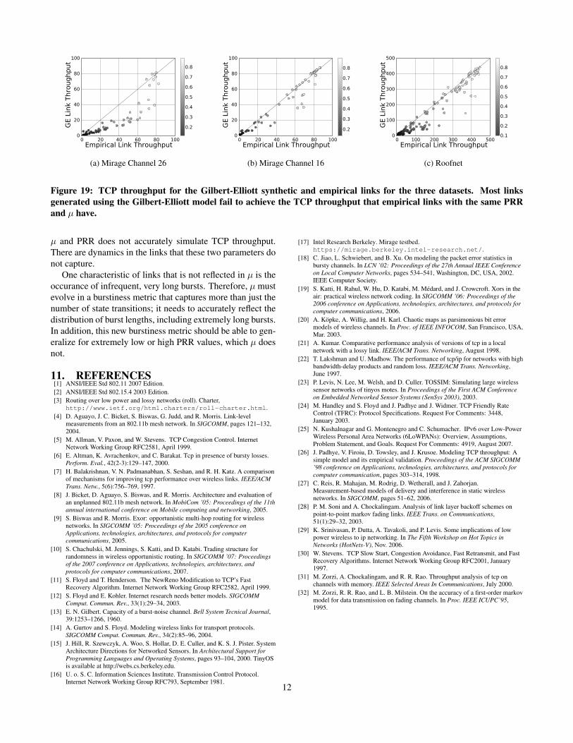
9.2 ResultsFigure 19 compares the TCP throughput values for the

empirical and simulated links for the different testbeds. In allthree figures, the x-axis shows the empirical TCP throughputand the y-axis the throughput for the link generated by theGilbert-Elliott model. Note that since the Roofnet data isevery 2ms instead of 10ms, the y-axis goes up to 500 packetsper second. The x = y is shown for reference – datapoints onthe line denote matched performance between simulated andreal-world links. This figure shows that synthesized linksperform very differently compared to the empirical data theytry to simulate.

For the Mirage channel 26 dataset, most datapoints fallunder the x = y line; simulated links have considerablylower TCP throughput. This leads to the conclusion thatlinks modeled using Gilbert-Elliott are not only quite differ-ent from empirical links, but also have a tendency to under-perform. Only about 12% of all links are within 10% of theirempirical partners. In the extreme cases, synthetic links canreport a throughput which is as much as 80% less than thatof real testbed measurements.

The results for Mirage channel 16 follow the same trend.About 50% of the links are within 10% of the empirical datatraces, while many have lower TCP throughput, as much as60% less. In the 802.11b experiments, we again see sim-ulated links with throughput that greately differs from theexpected – up to 80%.

Therefore while µ, as computed from a testbed trace, hasa good predictive value for TCP throughput, the reverse isnot true: simulation of a link using µ and the Gilbert-Elliottmodel is not accurate. More specifically, for our throughputmetric, synthetic links consistently underperform comparedto the empirical ones.

It must be that µ and TCP are correlated to a third vari-able, a characteristic that is currently missing from our ob-servations. More specifically, µ does not capture informationabout infrequently occuring long bursts of successes. This isa key ingredient in understanding the throughput that TCP’swindowing achieves due to the Additive Increase/Multiplica-tive Decrease scheme of congestion control. Very long burstsallow large size of the congestion window, larger flight size,and therefore, increased throughput.

Figure 20 shows the length of the longest burst of suc-cesses for each empirical link and its corresponding simu-lated link. If the Gilbert-Elliott model were to be used forsimulating wireless link behavior, we would expect data-points close to the 45-degree line. In reality, we discover

500 1000 1500 2000 2500Empirical Burst Length

500

1000

1500

2000

2500

Sim

ula

ted B

urs

t Le

ngth

Figure 20: About 50% of empirical links in the Miragechannel 26 data have maximum burst lengths that arelarger than the highest burst length the Gilbert-Elliottmodel ever produces.

that many empirical links have long bursts of successes thatthe Gilbert-Elliott model is unable to reproduce.

For example, over all 54 links from the Mirage channel 26data, the longest burst created by the Gilbert-Elliott model is149. At the same time, almost 50% of the empirical linkshave bursts much longer than that, up to 600 packets.

This observation explains why a Gilbert-Elliott syntheticlink cannot achieve a TCP throughput as high as that of anempirical link. A single burst on the order of hundreds ofpackets can cause a big difference in TCP’s windowing be-havior. Therefore, to be able to model and simulate links’behavior in terms of burstiness, future work must combinethe current version of µwith information about burst lengths.

10. Conclusion

This paper takes a first step towards extending the existinglexicon for describing wireless networks. While high-levelmetrics such as throughput and reception ratio can providesome coarse grained information, they are not enough to ac-curately describe a network. In Section 4 we saw that multi-ple TCP throughput values map to the same PRR, and mul-tiple PRRs to the same observed TCP performance. There-fore, simply reporting one or the other can lead to misleadingconclusions.

Observing links’ burstiness, i.e. the temporal correlationsof packet successes and losses, allowed us to refine our un-derstanding of link behavior. We used µ as a metric of bursti-ness and discovered that, when combined with PRR, it canreduce estimation error of TCP throughput by approximately50%. These results indicate that reporting a link burstinessmetric along with other network parameters can give a betterestimate of network performance.

While µ has a strong deductive value when computed onempirical links of intermediate reception ratios, it does notlend itself to simulations. Section 9 showed that using theGilbert-Elliot model to generate synthetic links with given

11

0 20 40 60 80 100Empirical Link Throughput

0

20

40

60

80

100

GE L

ink

Thro

ughput

0.2

0.3

0.4

0.5

0.6

0.7

0.8

(a) Mirage Channel 26

0 20 40 60 80 100Empirical Link Throughput

0

20

40

60

80

100

GE L

ink

Thro

ughput

0.2

0.3

0.4

0.5

0.6

0.7

0.8

(b) Mirage Channel 16

0 100 200 300 400 500Empirical Link Throughput

0

100

200

300

400

500

GE L

ink

Thro

ughput

0.1

0.2

0.3

0.4

0.5

0.6

0.7

0.8

(c) Roofnet

Figure 19: TCP throughput for the Gilbert-Elliott synthetic and empirical links for the three datasets. Most linksgenerated using the Gilbert-Elliott model fail to achieve the TCP throughput that empirical links with the same PRRand µ have.

µ and PRR does not accurately simulate TCP throughput.There are dynamics in the links that these two parameters donot capture.

One characteristic of links that is not reflected in µ is theoccurance of infrequent, very long bursts. Therefore, µ mustevolve in a burstiness metric that captures more than just thenumber of state transitions; it needs to accurately reflect thedistribution of burst lengths, including extremely long bursts.In addition, this new burstiness metric should be able to gen-eralize for extremely low or high PRR values, which µ doesnot.

11. REFERENCES[1] ANSI/IEEE Std 802.11 2007 Edition.[2] ANSI/IEEE Std 802.15.4 2003 Edition.[3] Routing over low power and lossy networks (roll). Charter,

http://www.ietf.org/html.charters/roll-charter.html.[4] D. Aguayo, J. C. Bicket, S. Biswas, G. Judd, and R. Morris. Link-level

measurements from an 802.11b mesh network. In SIGCOMM, pages 121–132,2004.

[5] M. Allman, V. Paxon, and W. Stevens. TCP Congestion Control. InternetNetwork Working Group RFC2581, April 1999.

[6] E. Altman, K. Avrachenkov, and C. Barakat. Tcp in presence of bursty losses.Perform. Eval., 42(2-3):129–147, 2000.

[7] H. Balakrishnan, V. N. Padmanabhan, S. Seshan, and R. H. Katz. A comparisonof mechanisms for improving tcp performance over wireless links. IEEE/ACMTrans. Netw., 5(6):756–769, 1997.

[8] J. Bicket, D. Aguayo, S. Biswas, and R. Morris. Architecture and evaluation ofan unplanned 802.11b mesh network. In MobiCom ’05: Proceedings of the 11thannual international conference on Mobile computing and networking, 2005.

[9] S. Biswas and R. Morris. Exor: opportunistic multi-hop routing for wirelessnetworks. In SIGCOMM ’05: Proceedings of the 2005 conference onApplications, technologies, architectures, and protocols for computercommunications, 2005.

[10] S. Chachulski, M. Jennings, S. Katti, and D. Katabi. Trading structure forrandomness in wireless opportunistic routing. In SIGCOMM ’07: Proceedingsof the 2007 conference on Applications, technologies, architectures, andprotocols for computer communications, 2007.

[11] S. Floyd and T. Henderson. The NewReno Modification to TCP’s FastRecovery Algorithm. Internet Network Working Group RFC2582, April 1999.

[12] S. Floyd and E. Kohler. Internet research needs better models. SIGCOMMComput. Commun. Rev., 33(1):29–34, 2003.

[13] E. N. Gilbert. Capacity of a burst-noise channel. Bell System Tecnical Journal,39:1253–1266, 1960.

[14] A. Gurtov and S. Floyd. Modeling wireless links for transport protocols.SIGCOMM Comput. Commun. Rev., 34(2):85–96, 2004.

[15] J. Hill, R. Szewczyk, A. Woo, S. Hollar, D. E. Culler, and K. S. J. Pister. SystemArchitecture Directions for Networked Sensors. In Architectural Support forProgramming Languages and Operating Systems, pages 93–104, 2000. TinyOSis available at http://webs.cs.berkeley.edu.

[16] U. o. S. C. Information Sciences Institute. Transmission Control Protocol.Internet Network Working Group RFC793, September 1981.

[17] Intel Research Berkeley. Mirage testbed.https://mirage.berkeley.intel-research.net/.

[18] C. Jiao, L. Schwiebert, and B. Xu. On modeling the packet error statistics inbursty channels. In LCN ’02: Proceedings of the 27th Annual IEEE Conferenceon Local Computer Networks, pages 534–541, Washington, DC, USA, 2002.IEEE Computer Society.

[19] S. Katti, H. Rahul, W. Hu, D. Katabi, M. Medard, and J. Crowcroft. Xors in theair: practical wireless network coding. In SIGCOMM ’06: Proceedings of the2006 conference on Applications, technologies, architectures, and protocols forcomputer communications, 2006.

[20] A. Kopke, A. Willig, and H. Karl. Chaotic maps as parsimonious bit errormodels of wireless channels. In Proc. of IEEE INFOCOM, San Francisco, USA,Mar. 2003.

[21] A. Kumar. Comparative performance analysis of versions of tcp in a localnetwork with a lossy link. IEEE/ACM Trans. Networking, August 1998.

[22] T. Lakshman and U. Madhow. The performance of tcp/ip for networks with highbandwidth-delay products and random loss. IEEE/ACM Trans. Networking,June 1997.

[23] P. Levis, N. Lee, M. Welsh, and D. Culler. TOSSIM: Simulating large wirelesssensor networks of tinyos motes. In Proceedings of the First ACM Conferenceon Embedded Networked Sensor Systems (SenSys 2003), 2003.

[24] M. Handley and S. Floyd and J. Padhye and J. Widmer. TCP Friendly RateControl (TFRC): Protocol Specifications. Request For Comments: 3448,January 2003.

[25] N. Kushalnagar and G. Montenegro and C. Schumacher. IPv6 over Low-PowerWireless Personal Area Networks (6LoWPANs): Overview, Assumptions,Problem Statement, and Goals. Request For Comments: 4919, August 2007.

[26] J. Padhye, V. Firoiu, D. Towsley, and J. Krusoe. Modeling TCP throughput: Asimple model and its empirical validation. Proceedings of the ACM SIGCOMM’98 conference on Applications, technologies, architectures, and protocols forcomputer communication, pages 303–314, 1998.

[27] C. Reis, R. Mahajan, M. Rodrig, D. Wetherall, and J. Zahorjan.Measurement-based models of delivery and interference in static wirelessnetworks. In SIGCOMM, pages 51–62, 2006.

[28] P. M. Soni and A. Chockalingam. Analysis of link layer backoff schemes onpoint-to-point markov fading links. IEEE Trans. on Communications,51(1):29–32, 2003.

[29] K. Srinivasan, P. Dutta, A. Tavakoli, and P. Levis. Some implications of lowpower wireless to ip networking. In The Fifth Workshop on Hot Topics inNetworks (HotNets-V), Nov. 2006.

[30] W. Stevens. TCP Slow Start, Congestion Avoidance, Fast Retransmit, and FastRecovery Algorithms. Internet Network Working Group RFC2001, January1997.

[31] M. Zorzi, A. Chockalingam, and R. R. Rao. Throughput analysis of tcp onchannels with memory. IEEE Selected Areas In Communications, July 2000.

[32] M. Zorzi, R. R. Rao, and L. B. Milstein. On the accuracy of a first-order markovmodel for data transmission on fading channels. In Proc. IEEE ICUPC’95,1995.

12