Provably Correct Derivation of Algorithms Using FermaT

Martin Ward and Hussein ZedanSoftware Technology Research Lab,

De Montfort University,Bede Island Building,

The Gateway,Leicester LE1 9BH, UK

martin@gkc.org.uk and zedan@dmu.ac.uk

Abstract

The transformational programming method of algorithm derivation starts with a formalspecification of the result to be achieved, plus some informal ideas as to what techniqueswill be used in the implementation. The formal specification is then transformed into animplementation, by means of correctness-preserving refinement and transformation steps, guidedby the informal ideas. The transformation process will typically include the following stages:(1) Formal specification (2) Elaboration of the specification, (3) Divide and conquer to handlethe general case (4) Recursion introduction, (5) Recursion removal, if an iterative solution isdesired, (6) Optimisation, if required. At any stage in the process, sub-specifications can beextracted and transformed separately. The main difference between this approach and theinvariant based programming approach (and similar stepwise refinement methods) is that loopscan be introduced and manipulated while maintaining program correctness and with no need toderive loop invariants. Another difference is that at every stage in the process we are workingwith a correct program: there is never any need for a separate “verification” step. These factorshelp to ensure that the method is capable of scaling up to the development of large and complexsoftware systems. The method is applied to the derivation of a complex linked list algorithmand produces code which is over twice as fast as the code written by Donald Knuth to solve thesame problem.

Contents

1 Introduction 2

1.1 Our Approach . . . . . . . . . . . . . . . . . . . . . . . . . . . . . . . . . . . . . . . . 41.2 Outline of the Algorithm Derivation method . . . . . . . . . . . . . . . . . . . . . . . 5

2 The WSL Language 7

3 Transformations Used in Derivations 10

4 Examples of Transformational Programming 15

4.1 Greatest Common Divisor . . . . . . . . . . . . . . . . . . . . . . . . . . . . . . . . . 154.1.1 Initial Program Derivation . . . . . . . . . . . . . . . . . . . . . . . . . . . . 164.1.2 Optimisation Transformations . . . . . . . . . . . . . . . . . . . . . . . . . . . 174.1.3 Alternate Program Derivation . . . . . . . . . . . . . . . . . . . . . . . . . . . 18

5 Knuth’s Polynomial Addition Algorithm 20

5.1 Abstract Polynomials . . . . . . . . . . . . . . . . . . . . . . . . . . . . . . . . . . . 205.2 Abstract Algorithm Derivation . . . . . . . . . . . . . . . . . . . . . . . . . . . . . . 215.3 Concrete Polynomials . . . . . . . . . . . . . . . . . . . . . . . . . . . . . . . . . . . 22

1

5.4 Algorithm Derivation . . . . . . . . . . . . . . . . . . . . . . . . . . . . . . . . . . . . 265.5 Execution Timings . . . . . . . . . . . . . . . . . . . . . . . . . . . . . . . . . . . . . 335.6 Polynomial Multiplication . . . . . . . . . . . . . . . . . . . . . . . . . . . . . . . . . 35

6 Conclusion 37

6.1 Software Evolution . . . . . . . . . . . . . . . . . . . . . . . . . . . . . . . . . . . . . 38

1 Introduction

The waterfall model of software development sees progress as flowing steadily downwards (like awaterfall) through the following stages:

1. Requirements Elicitation: analysing the problem domain and determining from the userswhat the program is required to do;

2. Design: developing the overall structure of the program;

3. Implementation: writing source code to implement the design in a particular programminglanguage;

4. Verification: running tests and debugging;

5. Maintenance: any modifications required after delivery to correct faults, improve perfor-mance, or adapt the product to a modified environment [06]

In theory, one proceeds from one phase to the next in a purely sequential manner. But in practice,at each stage in the process, information may be uncovered which affects previous stages. Forexample, during implementation it may be determined that the design is unsuitable and needsto be changed, during debugging the program implementation may have to be changed to fix thebugs, and so on. So the process described above will also require feedback loops from each stageto preceding stages.

It has long been recognised that while testing may increase our confidence in the correctness ofa program, no amount of testing can prove that a program is correct. As Dijkstra said: “Programtesting can be used to show the presence of bugs, but never to show their absence” [Dij70]. Toprove that a program is correct we need a precise mathematical specification which defines what theprogram is supposed to do, and a mathematical proof that the program satisfies the specification.

The program verification method of developing correct code involves writing code and thenverifying its correctness. A simple loop, for example, can be verified using the method of “loopinvariants”. This takes the following steps:

1. Determine the loop termination condition;

2. Determine the loop body;

3. Determine a suitable loop invariant;

4. Prove that the loop invariant is preserved by the loop body;

5. Determine a variant function for the loop;

6. Prove that the variant function is reduced by the loop body (thereby proving termination ofthe loop);

7. Prove that the combination of the invariant plus the termination condition satisfies thespecification for the loop.

2

However, loop invariants and postconditions can be difficult to determine with sufficient preci-sion, computing verification conditions can be tedious, and proving the correctness of verificationconditions can be difficult. Even with the aid of an automated proof assistant, there may still beseveral hundred remaining “proof obligations” to discharge (these are theorems which need to beproved in order to verify the correctness of the development) [BiM99, JJL91, NHW89]. In addition,should the implementation happen to be incorrect (i.e. the program has a bug), then the attemptat a proof is doomed to failure.

In a paper published in 1990, Sennett [Sen90] suggested that for “real” sized programs it wasimpractical to discharge more than a tiny fraction of the proof obligations. He presented a casestudy of the development of a simple algorithm, for which the implementation of one functiongave rise to over one hundred theorems which required proofs. Larger programs will require manymore proofs. However, since that time, there has been considerable research on the developmentof automated theorem provers (e.g. Event-B [ABH06]), which has led to a resurgence of interest inthe program verification approach in the form of a “posit and prove” style of programming. Notethat this approach still requires properties such as invariants and variants to be provided by thedevelopers [But06]. With improvements in automated theorem provers, a large proportion of proofobligations (POs) can be discharged automatically: but many still require user interaction whichoften requires (expensive) theorem proving experts [BGL11]. For commercial application this canbe thousands of proof obligations, requiring many man months or years of work. One industrialcase study using Event-B generated 300 POs, of which 100 required user intervention [BGL11].However, most of these may be handled using proof strategies leaving as few as 5%–10% of proofobligations which actually require manual proof.

An alternative to this a posteriori method, which was originally proposed by Dijkstra [Dij],is to control the process of program generation by constructing loop invariants in parallel withthe construction of the code. Combined with stepwise refinement [Dij70, Wir71], this approach isclaimed to scale up to fairly large programs.

A further refinement of this approach, called Invariant based programming, is to develop loopinvariants before the code itself is written. The idea has been proposed from the late 70’s byseveral researchers in different forms. Dijkstra’s later work on programming [Dij76] emphasises thedevelopment of a loop invariant as an important initial step before developing the body of the loop.Figure 1 summarises this approach. Notice that in the program verification method, Dijkstra’s

Pre/postconditions

Loop invariants

Program code

Verification

Figure 1: Invariant based programming

approach and the invariant based programming approach, the task of developing the loop invariantis moved to earlier and earlier phases in the process. Gries [Gri81] takes up the idea that a proof ofcorrectness and a program should be developed hand in hand. Back [Bac09] presents a notation for

3

writing invariant based programs, a method for finding invariants before writing code and methodsfor checking the correctness of invariant based programs. He points out that the natural structurefor the code may not be the same as the natural structure for the invariants and emphasises thatthe program should be structured around the invariants, so that the invariants are as simple aspossible, and therefore easier to manipulate: even if this results in more complicated code.

In all the development methods we have discussed so far, verification is the final step indevelopment. Up until the point where verification has been completed, the programmer cannotbe sure that the program is correct. Indeed, Back [Bac09] makes it clear that the program underdevelopment does not have to terminate or be free from deadlocks, and that the initial invariant isusually both incomplete and partially wrong. He stresses that it is essential to carefully check theconsistency of each transition when it is introduced.

1.1 Our Approach

In this paper we present a different method of programming, called transformational programmingor algorithm derivation. The method starts with a formal specification plus some informal ideasfor implementation techniques which might be useful. The formal specification is refined into acomplete program by applying a sequence of correctness-preserving refinement steps. The choiceof which transformation to apply at each stage is guided by the implementation ideas. Theseideas do not have to be formalised to any particular extent, since they are only used to selectbetween different transformations. The correctness of the transformation process guarantees thatthe transformed program is equivalent to the original. The method is summarised in Figure 2.

Formal

Program

Specification

Informal

Implementation

ideas

Program 1

Program n

Figure 2: Algorithm Derivation

Developing a program by stepwise transformation is an idea which dates back at least to the lateseventies, starting with Burstall and Darlington’s transformation work [BuD77, Dar78], the projectCIP (Computer-aided Intuition-guided Programming) [Bau79, BB85, BMP89, BaT87, Bro84] andcontinuing with the work of Morgan et al on the Refinement Calculus [Mor94, MRG88, MoV93]and the Laws of Programming [HHJ87]. However, the method presented here is very different fromthese. In the Refinement Calculus, the transformations for introducing and manipulating loopsrequire that any loops introduced must be accompanied by suitable invariant conditions and variantfunctions. Morgan says: “The refinement law for iteration relies on capturing the potentiallyunbounded repetition in a single formula, the invariant”, ([Mor94] p. 60, our emphasis). So, inorder to refine a statement to a loop, or, more generally, to introduce any loop into the program,

4

the developer still has to carry out all the steps 1–7 listed above for verifying the correctness of aloop.

In contrast with the refinement calculus, the method presented here does not require loopinvariants. We have transformations to introduce, manipulate and remove loops which do notdepend on the existence of loop invariants. Another key difference between Figure 2 and the othermethods is that there is no Verification step. This is because at each stage in the derivation processwe are working with a correct program. The program is always guaranteed to be equivalent tothe original specification, because it was derived from the specification via a sequence of proventransformations and refinements.

Over the last twenty-five years we have developed a powerful wide-spectrum specification andprogramming language, called WSL, together with a large catalogue of proven program trans-formations and refinements which can be used in algorithm derivations and reverse engineering.The method has been applied to the derivation of many complex algorithms from specifications,including the Schorr-Waite graph marking algorithm [War96], a hybrid sorting algorithm (anefficient combination of Quicksort and insertion sort) [War90], various tree searching algorithms[War99a] and a program slicing transformation [WaZ10]. The latter example shows that a programtransformation can itself be defined as a formal specification which can then be refined into animplementation of the transformation.

The transformation theory has also been used for reverse engineering and software migrationand forms the basis for the commercial FermaT software migration technology [War99b, War01,War04, WaZ05, WZH04].

1.2 Outline of the Algorithm Derivation method

A typical algorithm derivation takes the following steps:

1. Formal Specification: Develop a formal specification of the program, in the form of aWSL specification statement (see Section 2). This defines precisely what the program isrequired to accomplish, without necessarily giving any indication as to how the task is to beaccomplished. For example, a formal specification for the Quicksort algorithm for sorting thearray A[a . . b] is the statement SORT:

A[a . . b] := A′[a . . b].(sorted(A′[a . . b]) ∧ permutation(A[a . . b], A′[a . . b]))

This states that the array is assigned a new value which is sorted and also a permutation ofthe original value. The formula sorted(A) is defined:

∀1 6 i, j 6 ℓ(A). i 6 j ⇒ A[i] 6 A[j]

while permutation(A,B) is defined:

ℓ(A) = ℓ(B) ∧ ∃π : {1, . . . , ℓ(A)}→ {1, . . . , ℓ(A)}.∀1 6 i 6 ℓ(A). A[i] = B[π[i]]

where π : {1, . . . , ℓ(A)} → {1, . . . , ℓ(A)} means π is a bijection (a 1–1 and onto function)from the set {1, . . . , ℓ(A)} to itself.

The form of the specification should mirror the real-world nature of the requirements. It isa matter of constructing suitable abstractions such that local changes to the requirementsinvolve local changes to the specification.

The notation used for the specification should permit unambiguous expression of requirementsand support rigorous analysis to uncover contradictions and omissions. It should then bestraightforward to carry out a rigorous impact analysis of any changes.

The two most important characteristics of a specification notation are that it should permitproblem-oriented abstractions to be expressed, and that it should have rigorous semantics sothat specifications can be analysed for anomalies.

5

In [Dij72], Dijkstra writes:“In this connection it might be worthwhile to point out that thepurpose of abstracting is not to be vague, but to create a new semantic level in which onecan be absolutely precise.”

2. Elaboration: Elaborate the specification statement by taking out simple cases: for example,boundary values on the input or cases where there is no input data. These are applied bytransforming the specification statement, typically using the Splitting a Tautology transfor-mation (Transformation 1) followed by inserting assertions and then using the assertions torefine the appropriate copy of the specification to the trivial implementation. For Quicksort,an empty array or an array with a single element is already sorted, so SORT can be refinedas skip in these cases:

{a > b}; SORT ≈ {a > b}; skip

Elaboration will typically generate a somewhat larger program containing one or more copiesof the original specification statement.

3. Divide and Conquer: The general case is usually tackled via some form of “divide andconquer” strategy: this is where the informal implementation ideas come into play to directthe selection of transformations. For Quicksort the informal idea consists of two steps: (a)Partition the array around a pivot element: so that all the elements less than the pivot go onone side and the larger elements go on the other side. (b) Then the two sub-arrays are sortedusing copies of the original specification statement.

Divide and conquer will make the program still larger, often introducing more copies of thespecification statement.

At this point we still have a non-recursive program: so there are no induction proofs orinvariants required for the transformations. The proofs typically consist of a simple caseanalysis, plus analysis of the specification under certain restricted preconditions.

4. Recursion Introduction: The next step is to apply the Recursive Implementation (Trans-formation 5) to produce a recursive program with no remaining copies of the specification.This may be carried out in several stages, with each stage leaving fewer copies of thespecification statement, until all have been removed.

5. Recursion Removal: We now have an executable implementation of the specification. If aniterative implementation is required, then apply Recursion Removal (Transformation 8), or anappropriate special case of the transformation, to produce an iterative program. Again: thiscan be carried out in stages, or only partially: for example, tail recursion can be convertedto iteration, but inner recursive calls left in place.

6. Optimisation: Apply further optimising transformations as required.

The method is compositional at several levels:

1. At any stage in the development, any part of the program can be worked on in isolation andthe results “plugged back in” to the main program: this is due to the fact that refinement inWSL satisfies the replacement property [War89];

2. Different aspects of the development can often be handled separately: for example, correctnessand efficiency. We can derive a provably correct program and then apply various optimisingtransformations to improve its efficiency;

3. At any stage in the process we may use data transformations to change the data representationusing the “ghost variables” method [War94, War96, War93, War96] to convert abstract datastructures to concrete data structures.

6

These compositionality properties are important properties that any program development methodshould satisfy.

It should be noted that stages 1–3 of any transformational derivation involve analysing programswhich contain no recursion or iteration. This makes the analysis particularly straightforward: forexample, induction arguments are not needed. This is fortunate, as it is these stages which requirethe most input from the informal implementation ideas. Stages 4–6 involve standard transforma-tions for recursion introduction, recursion removal and optimisation. As the derivation progresses,the transformations involved become more generic and less domain-specific. The techniques ofcalculational programming [BiM96] may be relevant to these stages: these include rules such asfusion and tupling, generic maps, specialisations, abstract data types etc. In the later stages, theprogram will typically be getting larger, but the required transformations will become simpler andmore susceptible to automation. At some point, an optimising compiler will take over and generateexecutable code, or the code will be directly executed by an interpreter, as appropriate.

An important advantage of the transformational derivation approach, over the various “code andverify” approaches is that it enables a separation of concerns between implementing the algorithmand applying various optimisation techniques. Some of the optimisation transformations, recursionremoval for example (Transformation 8), produce code which is quite different in structure from theoriginal unoptimised code. This new structure is generated automatically by the transformationsequence. Using the “posit and prove” approach, the programmer would have to work out inadvance the structure of the optimised program: so that it can be “posited” as the next version.The programmer would also need to determine suitable loop invariants for the optimised code sothat it could be proved correct. This is not necessarily impossible, but could be difficult to carryout correctly for a large and complex program.

2 The WSL Language

WSL is a Wide Spectrum language in that the language covers the whole spectrum from veryhigh-level abstract specifications to detailed, low-level programming constructs. This means thatthe whole program derivation process can be carried out in a single language: we do not needseparate “specification” and “implementation” languages with the consequent difficulty of provingthe relationship between the two languages.

The WSL Language is constructed from a simple and tractable kernel language. New constructsare added to the language in a series of layers by means of definitional transformations. The mainlanguage layers are as follows, with each subsequent layer building on the previous layer:

• Kernel language;

• if statements, while loops;

• do . . . od loops and action systems;

• Procedures;

• Functions and expressions with side effects.

The syntax and semantics of the kernel language and higher levels of WSL have been describedin earlier papers [PrW94, War89, War04, WaZ07, YaW03] so will not be given here. In this paperwe make use of the following WSL language constructs:

• Skip: The statement skip terminates immediately without changing the value of any variable;

• Abort: The statement abort never terminates;

7

• Specification Statement: For any formula Q and list of variables x, let x′ be the corre-sponding list of primed variables. The statement x := x′.Q assigns new values to the variablesin x such that the condition Q becomes true. Within Q, x represents the original values ofx and x′ represents the new values. For example, the statement:

〈x, y〉 := 〈x′, y′〉.(x′ = y ∧ y′ = x)

swaps the values of variables x and y. The specification:

〈x〉 := 〈x′〉.(x′ = x2 − 2x + 2)

assigns x the value x2 − 2x + 2. The specification:

〈x〉 := 〈x′〉.(x′ = x′2 − 2x′ + 2)

will assign x the value 1 or 2 (with the particular value being chosen nondeterministically),while the specification:

〈x〉 := 〈x′〉.(x = x′2 − 2x′ + 2)

assigns x one of the two values: 1±√

x− 1

• Simple Assignment: For any variable v and expression e, the statement v := e is defined:

〈v〉 := 〈v′〉.(v′ = e)

• Deterministic Choice: if B1 then S1 elsif B2 then S2 . . . else Sn fi

• Nondeterministic Choice: if B1 → S1 ⊓⊔ . . . ⊓⊔ Bn → Sn fi

• While Loop: while B do S od

• Nondeterministic loop: do B1 → S1 ⊓⊔ . . . ⊓⊔ Bn → Sn od

• Floop: do S od The floop is an “unbounded” loop which is terminated by the execution ofa statement of the form exit(n) where n is a positive integer (not a variable or expression).exit(n) causes immediate termination of the n enclosing levels of nested floops. See [PrW94,War04] for more detailed discussion of these constructs and associated transformations.

• Recursive Statement: If S is any statement which contains occurrences of the symbol X assub-statements, then the statement (µX.S) is the recursive procedure whose body is S withX representing recursive calls to the procedure. For example, the while loop while B do S od

is equivalent to the recursive statement (µX.if B then S; X fi).

• Recursive procedures: A where statement contains a main body plus a collection of(possibly mutually recursive) procedures:

begin

S

where

proc F1(x1) ≡ S1.

. . .proc Fn(xn) ≡ Sn.

end

8

• Action System: An Action System is a set of parameterless mutually recursive procedurestogether with the name of the first action to be called. There may be a special action Z(with no body): call Z results in the immediate termination of the whole action system withexecution continuing with the next statement after the action system (if any). See [PrW94,War04] for more detailed discussion of action systems and associated transformations.

An action system has this syntax:

actions A1 :A1 ≡ S1.

A2 ≡ S2.

. . .An ≡ Sn. endactions

where, in this case, A1 is the starting action: so S1 is the first statement to be executed. Astatement of the form call Ai is a call to action Ai.

If the execution of any action body must lead to an action call, then the action systemis regular. In a regular action system, no call ever returns and the system can only beterminated by a call Z. A program written using labels and jumps translates directly into anaction system, provided all the labels appear at the top level (not inside a structure). Labelscan be promoted to the top level by introducing extra calls and actions, for example:

A : if B then L : S1 else S2 fi; S3

can be translated to the action system:

actions A :A ≡ if B then call L else call L2 fi.

L ≡ S1; call L3.

L2 ≡ S2; call L3.

L3 ≡ S3; call Z. endactions

So, using this “promotion” method, any program written using labels and jumps can betranslated directly into an action system. Any structured program can also be translateddirectly into an “unstructured” action system. For example, the while loop while B do S od

is equivalent to the regular action system:

actions A :A ≡ if B then S; call A else call Z fi. endactions

Recursive procedures and action systems are similar in several ways, the differences are:

• There is nothing in a where statement which corresponds to the Z action: all procedures mustterminate normally (and thus a “regular” set of recursive procedures could never terminate);

• Procedure calls can occur anywhere in a program, for example in the body of a while loop:action calls cannot occur as components of statements other than if statements and do . . . od

loops.

An action system which does not contain calls to Z can be translated to a where clause (theconverse is only true provided no procedure call is a component of a simple statement).

The nondeterministic programming constructs are based on Dijkstra’s guarded command lan-guage [Dij76].

9

3 Transformations Used in Derivations

In this section we list some of the main transformations which are used in algorithm derivations. Thesuccess of transformational programming is in a large part due to the development of a substantialcatalogue of proven transformations. These transformations are very widely applicable and can beused in many different situations.

There are various methods used to prove the correctness of a transformation, these include:

• A direct proof of the equivalence of the denotational semantics for the two programs;

• A proof based on the logical equivalence, or implication, between the corresponding weakestpreconditions. Given any program and a formula which defines a condition on the finalstate, the weakest precondition is the corresponding formula on the initial state such that ifthe program starts executing in a state satisfying the weakest precondition it is guaranteedto terminate in a state satisfying the given postcondition. In [War89] transformations areproved correct by using a “generic” postcondition in an extension of the logic. In [War04] weshow that two specific postconditions are sufficient to completely capture the semantics of aprogram.

• A proof based on induction over the set of truncations of the iterative or recursive constructsin the programs: see [War04] for details of the induction rules.

• A proof based on a sequence of existing transformations.

Many proofs use a combination of these methods. Although there has been some work on formal-ising the semantics and transformation proofs using the Coq Proof Assistant [ZMH02a, ZMH02b]most transformation proofs are manual. However, the work involved in proving a transformationonly has to be carried out once, while the transformation can be re-used in a huge number ofprogram derivations.

The first four transformations can be proved directly from the weakest preconditions (see[War89] Chapter One for the details).

Transformation 1 Splitting a TautologyIf B1 ∨ B2 is true then:

S ≈ if B1 → S ⊓⊔ B2 → S fi

For any formula B we have:S ≈ if B then S else S fi

These can be proved directly from the corresponding weakest preconditions: see [War89] Chap-ter One.

Transformation 2 Introduce assertions

if B then S1 else S2 fi ≈ if B then {B}; S1 else {¬B}; S2 fi

if B1 → S1 ⊓⊔ B2 → S2 fi ≈ if B1 → {B1}; S1 ⊓⊔ B2 → {B2}; S2 fi

Recall that an assertion in WSL is a statement, not an annotation of the program. Any transfor-mation which introduces an assertion is therefore guaranteeing that the condition in the assertionis always true at the point where the assertion is added.

Transformation 3 Append assertionIf the variables in x do not appear free in Q (i.e. the new value of x does not depend on the oldvalue) then:

x := x′.Q ≈ x := x′.Q; {Q[x/x′]}

10

where Q[x/x′] is the formula Q with every occurrence of a variable in x′ replaced by the corre-sponding variable in x. In particular, if x does not appear in the expression e, then:

x := e ≈ x := e; {x = e}

Transformation 4 Assignment MergingFor any variable x and expressions e1 and e2:

x := e1; x := e2 ≈ x := e2[e1/x]

Transformation 5 Recursive ImplementationSuppose we have a statement S′ which we wish to transform into the recursive procedure (µX.S).We claim that this is possible whenever:

1. The statement S′ is refined by S[S′/X] (which denotes S with all occurrences of X replaced byS′). In other words, if we replace recursive calls in S by copies of S′ then we get a refinementof S′;

2. We can find an expression t (called the variant function) whose value is reduced before eachoccurrence of S′ in S[S′/X].

Note that a refinement of a program is any program which is more defined (i.e. defined on at leastas many initial states as the original) and more deterministic (i.e. for each initial state on whichthe original program is defined, the refinement is also defined and has a smaller set of final states:therefore each of the final states for the refinement is an allowed final state for the original). If twoprograms are each a refinement of the other, then the programs are semantically equivalent.

The expression t need not be integer valued: any set Γ which has a well-founded order 4 issuitable. To prove that the value of t is reduced it is sufficient to prove that if t 4 t0 initially,then the assertion {t ≺ t0} can be inserted before each occurrence of S′ in S[S′/X]. The theoremcombines these two requirements into a single condition:

Theorem 3.1 The Recursive Implementation TheoremIf 4 is a well-founded partial order on some set Γ and t is a term giving values in Γ and t0 is a

variable which does not occur in S then if

{P ∧ t 4 t0}; S′ ≤ S[{P ∧ t ≺ t0}; S′/X]

then {P}; S′ ≤ (µX.S)

See [War89] Chapter One for the proof.

Transformation 6 Action call fold/unfoldIf S is any statement in an action system, one of whose actions is Ai ≡ Si., then:

S ≈ S[Si/call Ai]

This transformation can be used in either direction: to replace an action call by a copy of theaction body, or to replace a statement by a call to a suitable action body. In particular, let S beany statement in an action system (which is in a suitable position for a call to appear). Let An

be any new action name which is not already used in the system. Then we can add a new actionAn ≡ S. to the system: this transformation is trivial since the new action is unreachable. Nowapply Transformation 6 to replace S by call An.

See [War89] Chapter Four for the proof.

Transformation 7 Action Recursion RemovalLet Ai ≡ Si. be any action in a regular action system. Then we can remove “recursive” callscall Ai which appear in the action Ai ≡ Si. by the following process:

11

1. First enclose Si in a double-nested loop: do do Si; exit(2) od od

2. Next, replace each call Ai which appears in n nested loops by the statement exit(n + 1): soa call in Si which is not in any loops is replaced by exit(1), and so on.

Each call is therefore replaced by an exit which terminates the inner loop surrounding Si andre-iterates the outer loop, so that Si is executed again as required.

See [War89] Chapter Four for the proof.

The double loop is not always necessary: if all the recursive calls are in tail positions, then asingle loop is sufficient with the calls replaced by skip statements.

Transformation 8 Recursion RemovalSuppose we have a recursive procedure whose body is a regular action system in the followingform:

proc F (x) ≡actions A1 :A1 ≡ S1.

. . . Ai ≡ Si.

. . . Bj ≡ Sj0; F (gj1(x)); Sj1; F (gj2(x));. . . ; F (gjnj

(x)); Sjnj.

. . . endactions.

where Sj1, . . . ,Sjnjpreserve the value of x and no S contains a call to F (i.e. all the calls to F are

listed explicitly in the Bj actions) and the statements Sj0, Sj1, . . . ,Sjnj−1 contain no action calls.Note that, since the action system is regular, each of the statements Sjnj

must contain one or moreaction calls: in fact, they can only terminate by calling an action. There are M + N actions intotal: A1,. . . , AM , B1, . . . , BN . Note that the since the action system is regular, it can only beterminated by executing call Z which will terminate the current invocation of the procedure.

Our aim is to remove the recursion by introducing a local stack L which records “postponed”operations: When a recursive call to F (e) is required we “postpone” it by pushing the pair 〈0, e〉onto L (where e is the parameter required for the recursive call). Execution of the statements Sjk

also has to be postponed (since they occur between recursive calls), we record the postponementof Sjk and the current value of x, by pushing 〈〈j, k〉, x〉 onto L. Where the procedure body would

normally terminate (by calling Z) we instead call a new action F which pops the top item off Land carries out the postponed operation. If we call F with the stack empty then all postponedoperations have been completed and the procedure terminates by calling Z.

A recursive procedure in the form given above is equivalent to the following iterative procedurewhich uses a new local stack L and a new local variable m:

proc F ′(x) ≡var 〈L := 〈〉,m := 0〉 :

actions A1 :

A1 ≡ S1[call F /call Z].

. . . Ai ≡ Si[call F /call Z].

. . . Bj ≡ Sj0;L := 〈〈0, gj1(x)〉, 〈〈j, 1〉, x〉, 〈0, gj2(x)〉,

. . . , 〈0, gjnj(x)〉, 〈〈j, nj〉, x〉〉 ++ L;

call F .

. . . F ≡ if L = 〈〉then call Z

else 〈m,x〉 pop←− L;if m = 0 → call A1

12

⊓⊔ . . . ⊓⊔ m = 〈j, k〉→ Sjk[call F /call Z]; call F

. . . fi fi. endactions end.

where the substitutions Si[call F /call Z] are, of course, not applied to nested action systems whichare components of the Si.

See [War99a] for the proof, and some applications.

Within each Bj , at the point where F is called the top of the stack L is 〈0, gj1(x)〉. So this Fwill set x to gj1(x) and call Aj . We can therefore unfold F into Bj and simplify to get:

Bj ≡ Sj0;L := 〈〈〈j, 1〉, x〉, 〈0, gj2(x)〉,

. . . , 〈0, gjnj(x)〉, 〈〈j, nj〉, x〉〉 ++ L;

x := gj1;call Aj.

If nj = 1 for all j, then a value of the form 〈0, v〉 will never be pushed onto the stack, and each Bj

takes this form:

Bj ≡ Sj0;L := 〈〈〈j, 1〉, x〉〉 ++ L;x := gj1;call Aj.

If, in addition, the procedure is parameterless and there is only one B type action, then the onlyvalue pushed into the stack is 〈〈1, 1〉〉. So the stack can be replaced by a simple integer (whichrecords how many values were pushed onto the stack). So, for the special case of a parameterless,linear recursion we have:

proc F ≡actions A1 :A1 ≡ S1.

. . . Ai ≡ Si.

B1 ≡ S0; F ; S11. endactions.

is equivalent to:

proc F ′ ≡var 〈L := 0〉 :

actions A1 :

A1 ≡ S1[call F /call Z].

. . . Ai ≡ Si[call F /call Z].

. . . B1 ≡ Sj0; L := L + 1; call A1.

. . . F ≡ if L = 0then call Zelse L := L− 1;

S11[call F /call Z]; call F fi.

endactions end.

For example:

proc F ≡if B then S1 else S2; F ; S3 fi.

is equivalent to the iterative program:

13

proc F ′ ≡var 〈L := 0〉 :

actions A1 :

A1 ≡ if B then S1; call F else call B1 fi.

B1 ≡ S2; L := L + 1; call A1.

F ≡ if L = 0then call Zelse L := L− 1;

S3; call F fi. endactions end.

Remove the recursion in F , unfold into A1, unfold B1 into A1 and remove the recursion to give:

proc F ′ ≡var 〈L := 0〉 :

while ¬B do S2; L := L + 1 od;S1;while L 6= 0 do L := L− 1; S3 od.

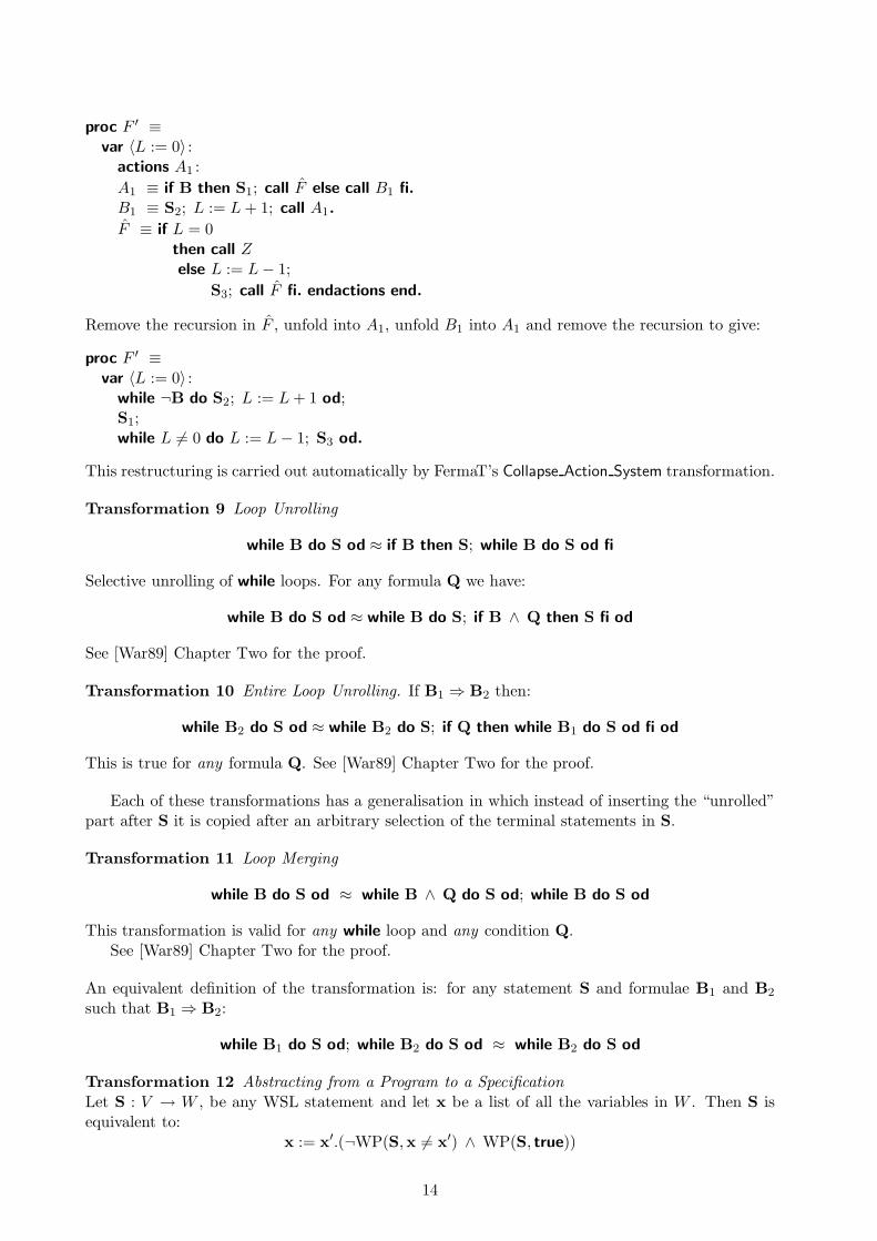
This restructuring is carried out automatically by FermaT’s Collapse Action System transformation.

Transformation 9 Loop Unrolling

while B do S od ≈ if B then S; while B do S od fi

Selective unrolling of while loops. For any formula Q we have:

while B do S od ≈ while B do S; if B ∧ Q then S fi od

See [War89] Chapter Two for the proof.

Transformation 10 Entire Loop Unrolling. If B1 ⇒ B2 then:

while B2 do S od ≈ while B2 do S; if Q then while B1 do S od fi od

This is true for any formula Q. See [War89] Chapter Two for the proof.

Each of these transformations has a generalisation in which instead of inserting the “unrolled”part after S it is copied after an arbitrary selection of the terminal statements in S.

Transformation 11 Loop Merging

while B do S od ≈ while B ∧ Q do S od; while B do S od

This transformation is valid for any while loop and any condition Q.See [War89] Chapter Two for the proof.

An equivalent definition of the transformation is: for any statement S and formulae B1 and B2

such that B1 ⇒ B2:

while B1 do S od; while B2 do S od ≈ while B2 do S od

Transformation 12 Abstracting from a Program to a SpecificationLet S : V → W , be any WSL statement and let x be a list of all the variables in W . Then S isequivalent to:

x := x′.(¬WP(S,x 6= x′) ∧ WP(S, true))

14

where for any program S and formula Q, the formula WP(S,Q) is the weakest precondition of S

on postcondition Q. This is the weakest condition on the initial state such that if S is started in astate which satisfies WP(S,Q) then it is guaranteed to terminate and the final state is guaranteedto satisfy Q. If S has any loops or recursion, then WP(S,Q) is defined as an infinite formula,so the specification statement will usually be infinitely large. But the transformation is still veryuseful during the “elaboration” and “divide and conquer” stages in the development process, andalso for analysing fragments of larger programs. See [War04] for the proof of this transformation.

In theory, this transformation solves all reverse engineering problems: since it defines an abstractspecification for any program [War04]. In practice, it is less useful because the specifications forprograms containing loops or recursion are infinite. But there are many programs and programfragments which do not contain loops or recursion: in one study [WZL08] over 40% of the modulesfrom a collection taken at random from several large assembler systems contained no loops.

Transformation 13 Refining a SpecificationGenerally, programmers find that a compound statement with assertions, if statements and simpleassignments to be easier to read and understand than the equivalent single specification state-ment. So we have implemented another transformation Refine Spec which analyses a specificationstatement and carries out the following operations:

1. Factor out any assertions: for example, if no variable in x′ appears free in P, then:

x := x′.(Q ∧ P) ≈ {P}; x := x′.Q

conversely, if no variable in x appears free in P then:

x := x′.(Q ∧ P) ≈ x := x′.Q; {P[x/x′]}

2. Expand into an if statement: for example, the specification x := x′.(Q ∨ (B ∧ P)) whereB does not contain any variables x′, is equivalent to

if B then x := x′.(Q′ ∨ P′) else x := x′.(Q′′) fi

where Q′ and P′ are the result of simplifying Q and P under the assumption that B istrue, and Q′′ is the result of simplifying Q under the assumption that B is false. Thesesub-specifications are then recursively refined;

3. Finally, any simple assignments or parallel assignments are extracted.

These transformations are proved in [War89] Chapter One.

4 Examples of Transformational Programming

A simple example of an algorithm derivation will demonstrate how the various transformationsintroduced in the previous section “fit together” to provide a complete derivation path from abstractspecification to efficient implementation. This example also shows that different informal ideascan drive the derivation process in different directions: resulting in a substantially different finalimplementation.

4.1 Greatest Common Divisor

The Greatest Common Divisor (GCD) of two numbers is the largest number which divides bothof the numbers with no remainder. A specification for a program which computes the GCD is thefollowing:

r := GCD(x, y)

15

where:GCD(x, y) = max

{

n ∈ N∣

∣ n|x ∧ n|y}

and n|x means “n divides x”. (Note that GCD(x, y) is undefined when both x and y are zero).It is easy to prove the following facts about GCD:

1. GCD(0, y) = y

2. GCD(x, 0) = x

3. GCD(x, y) = GCD(y, x)

4. GCD(x, y) = GCD(−x, y) = GCD(x,−y)

5. GCD(x, y) = GCD(x− y, y) = GCD(x, y − x) etc.

4.1.1 Initial Program Derivation

To refine our specification into a program, the obvious first step is to split a tautology on theconditions x = 0 and y = 0, using Fact (1) and Fact (2) respectively:

r := GCD(x, y) ≈ if x = 0 then r := yelsif y = 0

then r := xelse r := GCD(x, y) fi

Fact (3) does not appear to make much progress. If we restrict attention to non-negative integers,then Fact (4) does not apply. So we are left with Fact (5). If we take as our variant functionthe expression x + y, then, since we are restricted to non-negative integers, we can only transformr := GCD(x, y) to r := GCD(x− y, y) under the condition x > y. Similarly, for the condition y > xwe can transform r := GCD(x, y) to r := GCD(x, y − x). So we have the following elaboration ofthe specification:

if x = 0then r := y

elsif y = 0then r := x

elsif x > y then r := GCD(x− y, y)else r := GCD(x, y − x) fi

If x > y then x−y +y < x+y (since x and y are positive at this point) and similarly, if x < y thenx + y − x < x + y, so our variant function is reduced before each copy of the specification in theelaborated program. Applying Recursive Implementation (Transformation 5), we get the followingrecursive program:

proc gcd(x, y) ≡if x = 0

then r := yelsif y = 0

then r := xelsif x > y then r := gcd(x− y, y)

else r := gcd(x, y − x) fi end

This is a simple tail-recursion, so recursion removal (Transformation 8) produces this iterativeprogram:

16

proc gcd(x, y) ≡while x 6= 0 ∧ y 6= 0 do

if x > y then x := x− yelse y := y − x fi od;

if x = 0 then r := y else r := x fi end

This is essentially the same algorithm as Dijkstra produces by the method of invariants: exceptthat we have not needed to prove any invariants.

4.1.2 Optimisation Transformations

There is a problem with the algorithm in that, although it is correct, it is very inefficient whenx and y are very different in size. For example, if x = 1 and y = 231 then the program will take231 − 1 steps.

One solution would be to look for some other properties of GCD and generate a new, hopefullymore efficient, program which uses these properties. This requires throwing away the currentprogram: not a big issue in this case, since the program is so small. But in the case of a verylarge program, the suggestion that we throw it away and start again from scratch in order to solvea small efficiency problem is unlikely to be well received! Unfortunately, this is the only optionoffered by the “Invariant Based Programming” approach.

With the transformational programming approach, we have another option: attempt to trans-form the program in order to improve its efficiency. Consider the case where x is much larger thany. Then the statement x := x − y will be executed many times in succession. This suggests thatwe apply Entire Loop Unrolling (Transformation 10) to the program at the point just after thisassignment with the condition x > y. The result is:

proc gcd(x, y) ≡while x 6= 0 ∧ y 6= 0 do

if x > y then x := x− y;while x > y do

if x > ythen x := x− y fi od

else y := y − x fi od;r := x end

This simplifies to:

proc gcd(x, y) ≡while x 6= 0 ∧ y 6= 0 do

if x > y then while x > y do x := x− y od

else y := y − x fi od;if x = 0 then r := y else r := x fi end

Consider the inner while loop. This repeatedly subtracts y from x. Suppose the loop iterates qtimes (we know q > 0 since x > y initially). Then the final value of x is x = x0 − q.y where x0 wasthe initial value of x. We also have 0 6 x < y. These two facts show that the final value of x is infact the remainder obtained when x is divided by y. In other words:

while x > y do x := x− y od ≈ x := x mod y

when x > y initially.Similarly, entire loop unrolling can be applied after the assignment y := y − x and the same

optimisation applied to give:

17

proc gcd(x, y) ≡while x 6= 0 ∧ y 6= 0 do

if x > y then x := x mod yelse y := y mod x fi od;

if x = 0 then r := y else r := x fi end

We have transformed a program which was O(n) in execution time into an equivalent programwhich is O(log n)

4.1.3 Alternate Program Derivation

With a different informal idea and/or different constraints on the algorithm, the same derivationprocess will often produce a different result. For example, suppose the target machine does nothave a native integer division instruction, but does have efficient binary shift instructions. Ourinformal idea is to make use of the following additional information about the GCD function:

1. GCD(x, y) = 2.GCD(x/2, y/2) when x and y are both even;

2. GCD(x, y) = GCD(x/2, y) when x is even and y is odd;

3. GCD(x, y) = GCD(x, y/2) when x is odd and y is even;

4. GCD(x, y) = GCD((x− y)/2, y) when x and y are odd and x > y;

5. GCD(x, y) = GCD(x, (y − x)/2) when x and y are odd and y > x.

Applying Fact (1) above produces the following elaborated specification:

if x = 0 then r := yelsif y = 0 then r := xelsif 2|x ∧ 2|y

then r := 2.GCD(x/2, y/2)else r := GCD(x, y) fi

Applying Recursive Implementation (Transformation 5) plus Recursion Removal (Transforma-tion 8) to the first occurrence only of GCD produces:

if x = 0 then r := yelsif y = 0 then r := x

else var 〈L := 0〉 :while 2|x ∧ 2|y do

L := L + 1;x := x/2; y := y/2 od;

r := GCD(x, y);r := 2L.r end fi

Applying Fact (2) above, followed by Recursive Implementation (Transformation 5) and RecursionRemoval (Transformation 8) produces the following result:

if x = 0 then r := yelsif y = 0 then r := x

else var 〈L := 0〉 :while 2|x ∧ 2|y do

L := L + 1;x := x/2; y := y/2 od;

while 2|x do x := x/2 od;{x 6= 0 ∧ y 6= 0 ∧ ¬2|x};r := GCD(x, y);r := 2L.r end fi

18

We now focus attention on the case where x is known to be odd, and y is non-zero. Define:

GCDx(x, y) =DF{y 6= 0 ∧ ¬2|x}; r := GCD(x, y)

By Fact (3) we show that GCDx(x, y) is equivalent to:

while 2|y do y := y/2 od;GCDx(x, y)

Now apply Fact (4), and also Fact (3) from the first set of facts, to ensure that x is odd in everyoccurrence of GCDx:

while 2|y do y := y/2 od;if x = y then r := xelsif x > y then GCDx(y, (x− y)/2)

else GCDx(x, (y − x)/2) fi

Apply Recursive Implementation (Transformation 5) and Recursion Removal (Transformation 8):

do while 2|y do y := y/2 od;if x = y then r := x; exit fi;if x > y

then 〈x, y〉 := 〈y, x− y〉else y := y − x fi;

y := y/2 od

The final program is therefore:

if x = 0then r := y

elsif y = 0then r := xelse var 〈L := 0〉 :

while 2|x ∧ 2|y do

L := L + 1;x := x/2; y := y/2 od;

while 2|x do x := x/2 od;do while 2|y do y := y/2 od;

if x = y then r := x; exit fi;if x > y

then 〈x, y〉 := 〈y, x− y〉else y := y − x fi;

y := y/2 od

r := 2L.r end fi

If the CPU has an instruction which computes the ntz function (returning the number of terminatingzeros in the binary representation of the argument), and also efficient instructions for shifting binarynumbers, then three while loops can be implemented in straight-line code. For example, the firstwhile loop can be implemented as:

L := min(ntz(x), ntz(y));x := x/2L; y := y/2L;

An efficient method of computing the ntz function using de Bruijn sequences, was described in[LPR98].

19

5 Knuth’s Polynomial Addition Algorithm

In the introduction to Chapter Two of “Fundamental Algorithms” [Knu68] Knuth writes “AlthoughList processing systems are useful in a large number of situations, they impose constraints on theprogrammer that are often unnecessary; it is usually better to use the methods of this chapterdirectly in one’s own programs, tailoring the data format and the processing algorithms to theparticular application. . . .We will see that there is nothing magic, mysterious, or difficult aboutthe methods for dealing with complex structures; these techniques are an important part of everyprogrammer’s repertoire, and he can use them easily whether he is writing a program in assemblylanguage or in a compiler language like FORTRAN or ALGOL.”

He goes on to describe a data structure to implement multivariate polynomials using a four-waycircular-linked list structure. Using this data structure he presents an algorithm for polynomialaddition: given two polynomials, represented by pointers P and Q, which do not share any nodes,the algorithm adds polynomial P to polynomial Q, updating the structure for Q while leavingP unchanged. Despite Knuth’s confident assertion that “there is nothing. . . difficult about themethods”, the four-way linked list structure he used to implement polynomial addition turned outto be rather difficult to work with in practice. The algorithm is very complex and difficult to getright: there were at least three bugs in the version published in the first edition [Knu74].

We will use Knuth’s polynomial addition problem as a testbed for the transformational pro-gramming method applied to the derivation of complex linked-list algorithms. We will not makeany use of Knuth’s code (except to compare its efficiency with our generated code): instead we showthat simply following the derivation method leads to highly efficient code. Our derived algorithmturns out to be over twice as fast as Knuth’s in all test cases: and nearly four times faster in somecases.

A polynomial is either a constant or has the form:

∑

06j6n

gjxej

where x is a variable, n > 0, 0 = e0 < e1 < · · · < ej and gj are polynomials involving only variablesalphabetically less than x. Also, g1, . . . , gn are not zero.

5.1 Abstract Polynomials

For our first implementation of polynomial addition, we decided to suffer the constraints imposedby a list processing system by developing a WSL algorithm for polynomial addition which usesWSL sequences to implement polynomials. The WSL is compiled into Scheme code which in turnis compiled into C using the Hobbit Scheme compiler [Tam95].

A constant polynomial is represented as the singleton list 〈c〉 where c is an integer. Otherwise,a polynomial is represented as the list of three or more elements:

p = 〈x, 〈g0, e0〉, 〈g1, e1〉, . . . , 〈gn, en〉〉

Here, x is a string (the variable name), n > 0, 0 = e0 < e1 < · · · < en are the integer exponentsand gi are lists representing polynomials whose variables are all lexicographically less than x. Also,gj 6= 〈0〉 for all j > 0. The abstraction function abs(p) returns the polynomial represented by thelist p:

abs(p) =DF

{

p[1] if ℓ(p) = 1∑

06j6ℓ(p)−2 abs(p[j + 2][1]).p[1]p[j+2][2] otherwise

So, for example, for the list p = 〈x, 〈〈0〉, 0〉, 〈〈4〉, 1〉, 〈〈1〉, 2〉〉:

abs(p) = 0.x0 + 4.x1 + 1.x2

20

i.e.:abs(p) = x2 + 4.x

We call polynomials implemented as lists “abstract polynomials” and polynomials implementedas pointers “concrete polynomials”. The lists representing abstract polynomials have to satisfy thecondition I(p) where:

I(p) =DF

(ℓ(p) = 1 ∧ p[1] ∈ Z)∨

(

ℓ(p) > 3 ∧ p[1] ∈ Strings ∧ ∀v ∈ vars(p). (p[1] > v)∧ ℓ(p[2]) = 2 ∧ I(p[2][1]) ∧ p[2][2] = 0∧ ∀j : 3 6 j 6 ℓ(p). (ℓ(p[j]) = 2 ∧ I(p[j][1]) ∧ p[j][2] ∈ N

∧ p[j][2] > p[j − 1][2] ∧ p[j][1] 6= 〈0〉))

where Strings is the set of strings, and vars(p) is the set of variables used in the terms of polynomialp (i.e. all variables except the base variable):

vars(p) =DF

{

∅ if ℓ(p) = 1⋃

26j6ℓ(p) allvars(p[j][1]) otherwise

where:

allvars(p) =DF

{

∅ if ℓ(p) = 1

{p[1]} ∪⋃

26j6ℓ(p) allvars(p[j][1]) otherwise

With these definitions, the formal specification for a program which assigns r to the value of alist which represents a polynomial equal to abs(p) + abs(q) is simply:

add(r, p, q) =DF

r := r′.(I(r′) ∧ abs(r′) = abs(p) + abs(q))

5.2 Abstract Algorithm Derivation

With this data structure it is a simple task to derive a suitable recursive algorithm for adding twopolynomials. First, take out special cases: the obvious cases are when p and/or q are constantpolynomials (in which case, they are sequences of length 1):

add(r, p, q) ≈ if ℓ(p) = 1 then if ℓ(q) = 1 then r := 〈p[1] + q[1]〉else add(r, p, q[2][1]); r := 〈q[1], 〈r, 0〉〉 ++ q[3 . .] fi

elsif ℓ(q) = 1 then add(r, p[2][1], q); r := 〈q[1], 〈r, 0〉〉 ++ p[3 . .]else add(r, p, q) fi

Next, if p and q are polynomials in the same variable, then we add corresponding terms in thetwo sequences of terms. One slight complication is that if all the non-constant terms cancel, wemust make sure that we return the constant term rather than returning a constant polynomial (thisensures that the condition I(r′) is satisfied). Similarly, when adding two lists of terms, we musttake care not to generate a zero term when the exponent is non-zero.

After taking out all these cases, Recursive Implementation (Transformation 5) can be repeatedlyapplied to produce a set of mutually recursive procedures. These can be transformed into recursivefunctions using the definitional transformation for WSL functions:

funct Abs Add Poly(p, q) ≡(if ℓ(p) = 1

then if ℓ(q) = 1then 〈p[1] + q[1]〉else 〈q[1], 〈Abs Add Poly(p, q[2][1]), 0〉〉 ++ q[3 . .] fi

else if ℓ(q) = 1then 〈p[1], 〈Abs Add Poly(p[2][1], q), 0〉〉 ++ p[3 . .]

21

else if p[1] = q[1]then Abs Simplify(〈p[1]〉 ++ Abs Add Terms(p[2 . .], q[2 . .]))else if String Less?(p[1], q[1])

then 〈q[1], 〈Abs Add Poly(p, q[2][1]), 0〉〉 ++ q[3 . .]else 〈p[1], 〈Abs Add Poly(q, p[2][1]), 0〉〉 ++ p[3 . .] fi fi fi fi).;

The function Abs Add Terms takes two lists of terms (which are assumed to be in the same variable)and returns the result of adding the terms together:

funct Abs Add Terms(p, q) ≡(if p = 〈〉

then qelse if q = 〈〉

then pelse if p[1][2] = q[1][2]

then Abs Simplify Term(〈Abs Add Poly(p[1][1], q[1][1]), q[1][2]〉)++ Abs Add Terms(p[2 . .], q[2 . .])

else if p[1][2] < q[1][2]then 〈p[1]〉 ++ Abs Add Terms(p[2 . .], q)else 〈q[1]〉 ++ Abs Add Terms(p, q[2 . .]) fi fi fi fi).;

The function Abs Simplify simplifies a polynomial which has no terms apart from the constant termby returning the value in the constant term:

funct Abs Simplify(p) ≡(if ℓ(p) = 2

then p[2][1]else p fi).;

The function Abs Simplify Term returns an empty list if the term is zero, and otherwise returns asingleton list containing the term:

funct Abs Simplify Term(term) ≡(if term[2] > 0 ∧ term[1] = 〈0〉

then 〈〉else 〈term〉 fi).;

The code listed above was generated directly from the ASCII WSL code. After fixing a few typos,this code worked first time: this is in contrast to Knuth’s polynomial addition algorithm which hadat least three bugs in the published version [Knu74]. The abstract program was tested as follows:

1. First a few sample polynomials were used as test data and the results examined;

2. Then a small number of random polynomials were generated and used as test data and theresults examined;

3. Finally a huge number of polynomials were generated and tested by evaluating the polynomi-als with random values for the variables. The sum of the values for the two input polynomialswas compared with the value of the output polynomial.

5.3 Concrete Polynomials

Knuth’s algorithm for polynomial addition represents a polynomial using a complex linked structureof nodes or records. Each record has six fields:

1. UP is a pointer to the parent node in the tree (or the null pointer value Λ if this node is theroot of the whole polynomial);

22

• ••

• ••

Poly = g0 + g1xe1 + ... + gnx

en

• ••

...

g0 g1 gn

...

e1 en0

x •

Fields Poly = c (constant)

c Λ

UP

LEFT

EXP

CV DOWN

RIGHT

Figure 3: Representation of polynomials using four-directional links

2. DOWN is Λ for a constant polynomial, and otherwise a pointer to the first node in the list ofterms for this polynomial: this will be the term with a zero exponent;

3. LEFT and RIGHT are the pointers which form a doubly-linked circular list of terms. Theterms are linked in order of exponent, there is always a term with a zero exponent, and theterm with the highest exponent links back to the zero exponent term via its RIGHT pointer.Each list contains at least two terms (otherwise we would have a constant polynomial: andthis variable would be redundant);

4. CV is either the constant value for a constant polynomial (which has DOWN set to Λ) or thename of the variable for a non-constant polynomial (in which case DOWN points to the termwith a zero exponent in the list of terms);

5. EXP is the exponent value for this term. Note that the variable which has this exponentis given by the CV value of the node pointed at by UP: the CV value for this node is theconstant value or variable name for this term’s coefficient.

Figure 3 illustrates how the data structure is used to represent both a constant and a non-constantpolynomial. The crossed-out values are irrelevant.

We have implemented Knuth’s algorithm in WSL, using a set of arrays U,D,L,R,C and Eto implement the fields UP, DOWN, LEFT, RIGHT, CV and EXP respectively in the records, withpointers represented as indices in these arrays. The special value Λ represents a “null pointer”, asin Knuth’s code. For a constant polynomial (where D[P ] = Λ) C[P ] contains the integer value andthe other array values are irrelevant. Otherwise, C[P ] contains the variable name, and D[P ] pointsto the head of a circular-linked list of terms. The first term D[P ] has E[D[P ]] = 0 and C[D[P ]]is the constant polynomial, R[D[P ]] points to the next term (which has an E value greater thanzero), and so on. The L fields point back to the previous term in the list, creating a doubly-linkedlist, and the U fields point to the parent polynomial, also creating a doubly-linked list. The R field

23

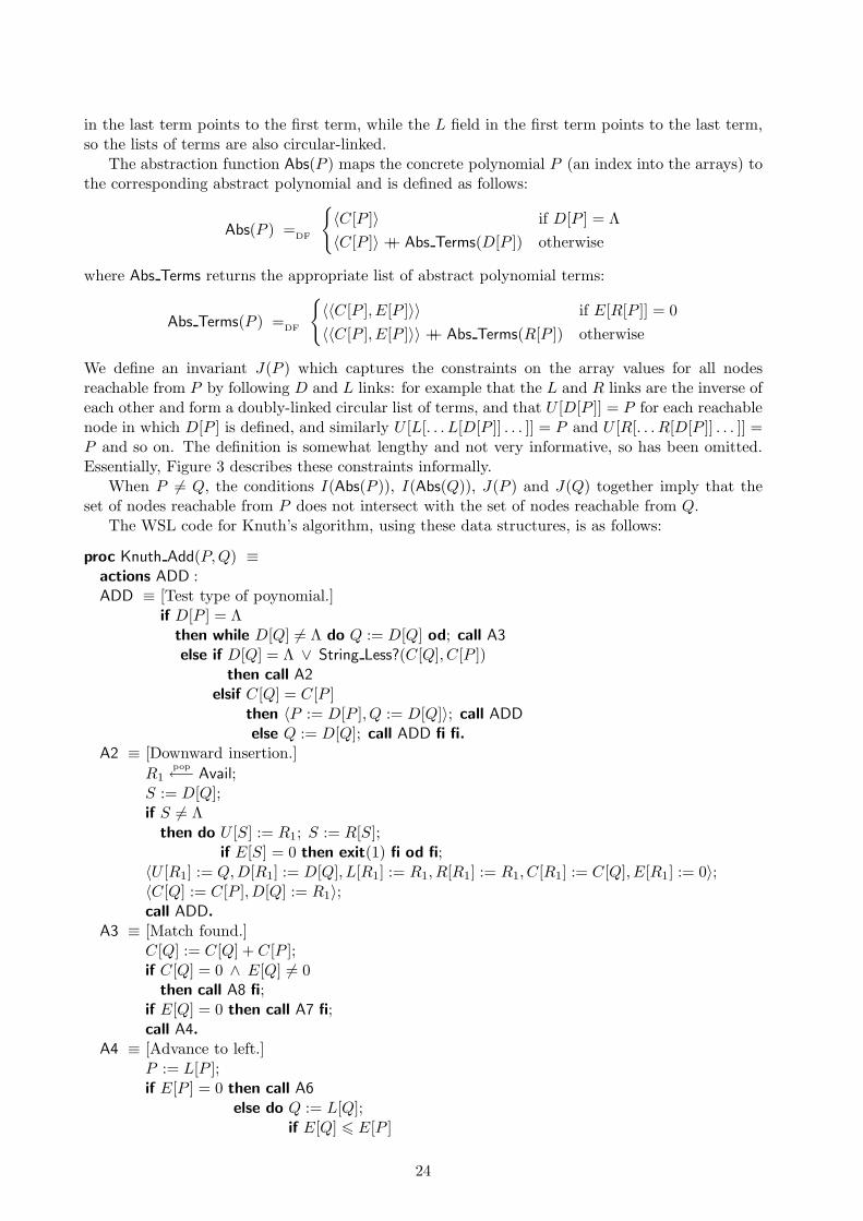
in the last term points to the first term, while the L field in the first term points to the last term,so the lists of terms are also circular-linked.

The abstraction function Abs(P ) maps the concrete polynomial P (an index into the arrays) tothe corresponding abstract polynomial and is defined as follows:

Abs(P ) =DF

{

〈C[P ]〉 if D[P ] = Λ

〈C[P ]〉 ++ Abs Terms(D[P ]) otherwise

where Abs Terms returns the appropriate list of abstract polynomial terms:

Abs Terms(P ) =DF

{

〈〈C[P ], E[P ]〉〉 if E[R[P ]] = 0

〈〈C[P ], E[P ]〉〉 ++ Abs Terms(R[P ]) otherwise

We define an invariant J(P ) which captures the constraints on the array values for all nodesreachable from P by following D and L links: for example that the L and R links are the inverse ofeach other and form a doubly-linked circular list of terms, and that U [D[P ]] = P for each reachablenode in which D[P ] is defined, and similarly U [L[. . . L[D[P ]] . . . ]] = P and U [R[. . . R[D[P ]] . . . ]] =P and so on. The definition is somewhat lengthy and not very informative, so has been omitted.Essentially, Figure 3 describes these constraints informally.

When P 6= Q, the conditions I(Abs(P )), I(Abs(Q)), J(P ) and J(Q) together imply that theset of nodes reachable from P does not intersect with the set of nodes reachable from Q.

The WSL code for Knuth’s algorithm, using these data structures, is as follows:

proc Knuth Add(P,Q) ≡actions ADD :ADD ≡ [Test type of poynomial.]

if D[P ] = Λthen while D[Q] 6= Λ do Q := D[Q] od; call A3

else if D[Q] = Λ ∨ String Less?(C[Q], C[P ])then call A2

elsif C[Q] = C[P ]then 〈P := D[P ], Q := D[Q]〉; call ADD

else Q := D[Q]; call ADD fi fi.

A2 ≡ [Downward insertion.]

R1pop←− Avail;

S := D[Q];if S 6= Λ

then do U [S] := R1; S := R[S];if E[S] = 0 then exit(1) fi od fi;

〈U [R1] := Q,D[R1] := D[Q], L[R1] := R1, R[R1] := R1, C[R1] := C[Q], E[R1] := 0〉;〈C[Q] := C[P ],D[Q] := R1〉;call ADD.

A3 ≡ [Match found.]C[Q] := C[Q] + C[P ];if C[Q] = 0 ∧ E[Q] 6= 0

then call A8 fi;if E[Q] = 0 then call A7 fi;call A4.

A4 ≡ [Advance to left.]P := L[P ];if E[P ] = 0 then call A6

else do Q := L[Q];if E[Q] 6 E[P ]

24

then exit(1) fi od;if E[P ] = E[Q] then call ADD fi fi;

call A5.

A5 ≡ [Insert to right.]

R1pop←− Avail;

〈U [R1] := U [Q],D[R1] := Λ, L[R1] := Q,R[R1] := R[Q]〉;L[R[R1]] := R1; R[Q] := R1;〈E[R1] := E[P ], C[R1] := 0〉; Q := R1;call ADD.

A6 ≡ [Return upward.]P := U [P ]; call A7.

A7 ≡ [Move Q up to right level.]if U [P ] = Λ

then call A11

else while C[U [Q]] 6= C[U [P ]] do Q := U [Q] od;call A4 fi.

A8 ≡ [Delete zero term.]R1 := Q; Q := R[R1]; S := L[R1]; R[S] := Q; L[Q] := S;

Availpush←− R1;

if E[L[P ]] = 0 ∧ Q = Sthen call A9 else call A4 fi.

A9 ≡ [Delete constant polynomial.]R1 := Q;Q := U [Q];〈D[Q] := D[R1], C[Q] := C[R1]〉;Avail

push←− R1;S := D[Q];if S 6= Λ then do U [S] := Q; S := R[S];

if E[S] = 0 then exit(1) fi od fi;call A10.

A10 ≡ [Zero detected?]if D[Q] = Λ ∧ C[Q] = 0 ∧ E[Q] 6= 0

then P := U [P ]; call A8 else call A6 fi.

A11 ≡ [Terminate.]while U [Q] 6= Λ do Q := U [Q] od; call Z. endactions.;

Here, Avail is the list of free nodes, R1pop←− Avail takes a free node from the list and returns its

pointer in R1, and Availpush←− R1 returns the node pointed at by R1 to the free list.

Later, in [Knu74] Knuth wrote: “I also know of places where I have myself used a complicatedstructure with excessively unrestrained goto statements, especially the notorious Algorithm 2.3.3Afor multivariate polynomial addition [Knu68]. The original program had at least three bugs;exercise 2.3.3–14, ‘Give a formal proof (or disproof) of the validity of Algorithm A,’ was thereforeunexpectedly easy. Now, in the second edition, I believe that the revised algorithm is correct, but Istill don’t know any good way to prove it; I’ve had to raise the difficulty rating of exercise 2.3.3–14,and I hope someday to see the algorithm cleaned up without loss of its efficiency.”

In a previous paper [War94] we proved the correctness of the above algorithm by transformingit into a suitable recursive procedure, applying our recursion removal theorem in reverse (in orderto introduce recursion) and then changing the data representation from concrete polynomials tothe corresponding abstract polynomials. So we were not surprised to find that the above programis indeed correct!

We were hopeful that the abstract algorithm would not be too inefficient, compared to Knuth’salgorithm: in fact we suspected that the abstract algorithm might even be more efficient in some

25

cases. Extensive testing with various sizes of random polynomials demonstrated that the abstractalgorithm was in reality more efficient than Knuth’s algorithm for every case tested!

With small polynomials (up to two variables and up to four terms at each level), the abstractalgorithm was only 14% faster than Knuth’s algorithm. As the polynomial size increased, theabstract algorithm became increasingly more efficient: with up to seven variables and up to fourterms at each level the abstract algorithm was three times faster. For very large polynomials (up toseven variables and up to 20 terms at each level) the abstract algorithm is about 750 times faster!See Section 5.5 for detailed timing results.

The dramatic speed advantage of the abstract algorithm on large polynomials is due to thefact that the abstract algorithm can “share” data structures, or parts of data structures. Knuth’salgorithm, although it apparently saves space by updating Q in place, cannot allow the result Qto share any nodes with polynomial P , due to the various “reverse pointers” (the “up” and “left”pointers in the linked lists). So, for example, adding a large polynomial P to a constant polynomialQ results in the creation of a complete copy of P : while the result for the abstract algorithm canshare sub-structures with the parameters. Knuth’s algorithm destroys the original polynomial inQ, while for the abstract algorithm, the original data structure is available via the original pointer.If it is not needed then any unshared nodes will be garbage-collected.

With regard to memory consumption: the abstract algorithm requires additional memory tostore the recursion stack. In the worst case, the stack length is proportional to the size of thepolynomial. However, each node in the abstract polynomial contains only two pointers, while thenodes in Knuth’s polynomials contain four pointers. So the abstract algorithm will actually use lessmemory in most, if not all, cases: especially in cases where sub-trees can be shared. For example,in the abstract representation of the polynomial:

(x2 + 2x + 3)z2 + (x2 + 2x + 3)z + 4

the pointers to the coefficients for z2 and z could point to the same location: which contains asingle copy of the representation of x2 + 2x + 3.

To be fair to Knuth, he does not claim that his algorithm is the best: “No claim is being madehere that the representation shown in Fig. 28 is the “best” for polynomials in several variables; . . .Our main interest in Algorithm A is the way it typifies manipulations on trees with many links.”[Knu68]. On the other hand, if this algorithm really “typifies manipulations on trees with manylinks”, perhaps the conclusion to be drawn from these empirical results is that trees with manylinks (in particular: doubly-linked circular lists) should be avoided wherever possible! By usingstandard list structures in a language with garbage collection, many link manipulations can beavoided and components of larger data structures can be shared. This sharing of data structureswould be especially valuable in programs which manipulate a large number of polynomials.

5.4 Algorithm Derivation

In the rest of this section we will apply the transformational programming method to derive animplementation of polynomial addition which uses Knuth’s data structures. Our specification istherefore:

ADD(P,Q) =DF〈U,D,L,R,E,C〉 := 〈U ′,D′, L′, R′, E′, C ′〉.

Abs′(P ) = Abs(P ) ∧ abs(Abs′(Q)) = abs(Abs(P )) + abs(Abs(Q))∧ I(Abs(P )) ∧ I(Abs(Q)) ∧ I(Abs′(Q))∧ J(P ) ∧ J(Q) ∧ J ′(Q)

where Abs′ is the analogue of the Abs function defined on U ′, D′, . . . etc., and J ′ is the correspondinganalogue of J .

26

With this specification, we start the derivation process in the usual way by taking out thespecial cases. If D[P ] = Λ then Abs(P ) is a constant polynomial:

ADD(P,Q) ≈ if D[P ] = Λ then ADD CONST(C[P ], Q) else ADD(P,Q) fi

where: ADD CONST adds a constant to a polynomial. The specification for ADD CONST can beelaborated as:

ADD CONST(c,Q) ≈ if D[Q] = Λthen C[Q] := C[Q] + celse Q := D[Q]; ADD CONST(c,Q); Q := U [Q] fi

This can be converted to a recursive procedure: but will need a stack, or at least a recursion depthcounter, to remove the recursion, since the inner copy of ADD CONST is not in a tail position, dueto the need to restore the original value of Q. However, if we make c and Q parameters, then wedo not need to restore their values. Applying the recursion introduction theorem to ADD CONST

gives a tail-recursive procedure which can be converted to a loop:

proc add const(c,Q) ≡while D[Q] 6= Λ do Q := D[Q] od;C[Q] := C[Q] + c.

We can therefore refine ADD as follows:

ADD(P,Q) ≤ if D[P ] = Λ then add const(C[P ], Q)else ADD(P,Q) fi

If D[P ] 6= Λ but D[Q] = Λ then we need to create a copy of the entire polynomial P , and then addthe original constant value of Q to the copy of P . The specification for this copy operation is:

COPY(P,Q) =DF〈U,D,L,R,E,C〉 := 〈U ′,D′, L′, R′, E′, C ′〉.

Abs′(P ) = Abs(P ) ∧ Abs′(Q)) = Abs(P ))∧ I(Abs(P )) ∧ I(Abs(Q)) ∧ I(Abs′(Q))∧ J(P ) ∧ J(Q) ∧ J ′(Q)

We will now elaborate on this specification.If P is a constant polynomial, then we just copy the constant and exponent to Q. Otherwise, we

create a suitable doubly-linked list of nodes and copy each of the children of P into these nodes:

COPY(P,Q) ≤ C[Q] := C[P ]; E[Q] := E[P ];if D[P ] = Λ

then D[Q] := Λ

else P := D[P ]; R1pop←− Avail; D[Q] := R1; U [R1] := Q; Q := R1;

do COPY(P,Q);if E[R[P ]] = 0 then S := D[U [Q]]; R[Q] := S; L[S] := Q; exit fi;P := R[P ];

R1pop←− Avail; U [R1] := U [Q]; L[R1] := Q; R[Q] := R1; Q := R1 od;

Q := U [Q]; P := U [P ] fi

At the copy of the specification in the elaborated version (on the right), the size of P has beenreduced. So we can apply Recursive Implementation (Transformation 5) to get a recursive proce-dure. To remove the recursion using Recursion Removal (Transformation 8), first restructure thebody of the recursive procedure as a regular action system:

27

proc copy(P,Q) ≡actions A :A ≡ C[Q] := C[P ]; E[Q] := E[P ];

if D[P ] = Λthen D[Q] := Λ; call Z

else P := D[P ]; R1pop←− Avail; D[Q] := R1; U [R1] := Q; Q := R1; call B1 fi.

B1 ≡ copy(P,Q); call A1.

A1 ≡ if E[R[P ]] = 0then var 〈S := D[U [Q]]〉 : R[Q] := S; L[S] := Q end; Q := U [Q]; P := U [P ]; call Zelse P := R[P ];

R1pop←− Avail; U [R1] := U [Q]; L[R1] := Q; R[Q] := R1; Q := R1;

call B1 fi. endactions.

For the recursion removal, we can avoid using a stack by noting that:

• The values of P and Q are preserved over the body of COPY(P,Q); and

• On returning from a call to COPY, if P has its original value, then this is the initial call,otherwise it is a recursive call.

Using these facts, and Recursion Removal (Transformation 8) we derive the following iterativeprocedure:

proc copy(P,Q) ≡var 〈P0 := P 〉 :

actions A :A ≡ C[Q] := C[P ]; E[Q] := E[P ];

if D[P ] = Λ

then D[Q] := Λ; call A

else P := D[P ]; R1pop←− Avail; D[Q] := R1; U [R1] := Q; Q := R1; call B1 fi.

B1 ≡ call A.

A ≡ if P = P0 then call Zelse call A1 fi.

A1 ≡ if E[R[P ]] = 0

then var 〈S := D[U [Q]]〉 : R[Q] := S; L[S] := Q end; Q := U [Q]; P := U [P ]; call Aelse P := R[P ];

R1pop←− Avail; U [R1] := U [Q]; L[R1] := Q; R[Q] := R1; Q := R1;

call B1 fi. endactions end.

The iterative algorithm was restructured automatically, using the FermaT Maintenance Environ-ment (see Section 6) to produce the following structured code:

proc copy(P,Q) ≡var 〈P0 := P 〉 :

do do C[Q] := C[P ]; E[Q] := E[P ];if D[P ] = Λ then exit(1) fi;

P := D[P ]; R1pop←− Avail; D[Q] := R1; U [R1] := Q; Q := R1 od;

D[Q] := Λ;do if P = P0 then exit(2) fi;

if E[R[P ]] 6= 0 then exit(1) fi;var 〈S := D[U [Q]]〉 : R[Q] := S; L[S] := Q end;Q := U [Q]; P := U [P ] od;

P := R[P ]; R1pop←− Avail; U [R1] := U [Q]; L[R1] := Q; R[Q] := R1; Q := R1 od end end

28

This code worked first time when it was tested.We therefore have the following refinement of ADD:

ADD(P,Q) ≤ if D[P ] = Λ then add const(C[P ], Q)elsif D[Q] = Λ then var 〈c := C[Q]〉 : COPY(P,Q); add const(c,Q) end

elsif C[Q] > C[P ] then ADD(P,Q)elsif C[Q] < C[P ] then ADD(P,Q)

else ADD(P,Q) fi

For the case where C[Q] > C[P ] we simply need to add Q to the constant element of P :

{C[Q] > C[P ]}; ADD(P,Q) ≤ {C[Q] > C[P ]}; Q := D[Q]; ADD(P,Q); Q := U [Q]

For the case where C[Q] = C[P ], we simply need to add the two lists of terms together as follows:

P := D[P ]; Q := D[Q]; ADD TERMS(P,Q); P := U [P ]; Q := U [Q]

where ADD TERMS adds the corresponding terms in the two polynomials, given that P and Qpoint to the first term in the list. Its implementation will be discussed below.

If C[Q] < C[P ] we need to convert Q to a constant polynomial with the same variable as Pby inserting a new parent node, after which we can add the terms of P to the terms of this newpolynomial:

R1pop←− Avail; C[R1] := C[P ]; D[R1] := Q; U [R1] := U [Q];

E[R1] := E[Q]; E[Q] := 0; L[R1] := L[Q]; R[R1] := R[Q];U [Q] := R1; L[Q] := Q; R[Q] := Q;P := D[P ]; ADD TERMS(P,Q); P := U [P ]; Q := U [Q]

We can implement ADD TERMS as a simple loop which uses ADD to add each term. After addingtwo terms, we need to check if the result has a zero coefficient with non-zero exponent. Theseterms are not allowed by the assertion I on the abstract version of the polynomial. Similarly, afteradding all the terms, we need to check if the result is a constant polynomial (i.e. all the terms withnon-zero exponent ended up with a zero coefficient and therefore were deleted). In this case, weneed to replace the polynomial by the constant (its first term). The specification ADD TERMS canassume that P and Q have the same exponent:

ADD TERMS(P,Q) ≈ ADD(P,Q);C : Check for a zero term with non-zero exponent;if E[Q] 6= 0 ∧ D[Q] = Λ ∧ C[Q] = 0

then var 〈R1 := Q,S := R[Q]〉 :Q := L[Q]; L[S] := Q; R[Q] := S;

Availpush←− R1 end fi;

ADD REST(P,Q)

The statement ADD REST(P,Q) will move Q to the appropriate term, and then continue addingterms. If there is no appropriate term (a term with the same exponent as E[P ]) then we needto insert a node in the list of terms and copy P over this node. We can then add the rest of theterms:

ADD REST(P,Q) ≈ P := R[P ];if E[P ] 6= 0

then Q := R[Q];while E[Q] > 0 ∧ E[Q] < E[P ] do Q := R[Q] od;if E[Q] = E[P ]

then ADD TERMS(P,Q)

29

else C : Insert a copy of P to the left of Q;var 〈R1 := 0〉 :

R1pop←− Avail;

L[R1] := L[Q]; R[R1] := Q; U [R1] := U [Q]; E[R1] := E[P ];R[L[Q]] := R1; L[Q] := R1; Q := R1 end;

copy(P,Q);ADD REST(P,Q) fi

This specification for ADD REST is tail-recursive, so it can be converted to a loop. Unfolding thisloop into the specification for ADD TERMS results in another tail-recursive specification, whichagain can be converted to a loop:

proc add terms(P,Q) ≡do ADD(P,Q);

C : Check for a zero term with non-zero exponent;if E[Q] 6= 0 ∧ D[Q] = Λ ∧ C[Q] = 0

then var 〈R1 := Q,S := R[Q]〉 :Q := L[Q]; L[S] := Q; R[Q] := S;

Availpush←− R1 end fi;

do P := R[P ];if E[P ] = 0 then exit(2) fi;Q := R[Q];while E[Q] > 0 ∧ E[Q] < E[P ] do Q := R[Q] od;if E[Q] = E[P ] then exit(1) fi;C : Insert a copy of P to the left of Q;var 〈R1 := 0〉 :

R1pop←− Avail;

L[R1] := L[Q]; R[R1] := Q; U [R1] := U [Q]; E[R1] := E[P ];R[L[Q]] := R1; L[Q] := R1; Q := R1 end;

copy(P,Q) od od.

Putting all these implementations together, and applying Recursive Implementation (Transfor-mation 5), we derive the following recursive implementation of ADD:

proc add(P,Q) ≡if D[P ] = Λ

then add const(C[P ], Q)elsif D[Q] = Λ

then var 〈c := C[Q]〉 : copy(P,Q); add const(c,Q) end

elsif C[Q] > C[P ]then Q := D[Q]; add(P,Q)else insert below Q;

P := D[P ]; Q := D[Q];do add(P,Q);

check for zero term;do P := R[P ];

if E[P ] = 0 then exit(2) fi;Q := R[Q];while E[Q] > 0 ∧ E[Q] < E[P ] do Q := R[Q] od;if E[Q] = E[P ] then exit fi;insert copy od od;

P := U [P ];check for const poly fi.

30

proc add const(c,Q) ≡while D[Q] 6= Λ do Q := D[Q] od;C[Q] := C[Q] + c.

proc insert below Q ≡if C[Q] < C[P ]

then C : Insert a node below Q and convert Q to a constant poly;var 〈R1 := 0, S := D[Q]〉 :

R1pop←− Avail; ;

do U [S] := R1; S := R[S];if E[S] = 0 then exit(1) fi od;

U [R1] := Q; D[R1] := S; L[R1] := R1; R[R1] := R1;C[R1] := C[Q]; E[R1] := 0; C[Q] := C[P ]; D[Q] := R1 end fi.

proc check for zero term ≡C : Check for a zero term with non-zero exponent;if E[Q] 6= 0 ∧ D[Q] = Λ ∧ C[Q] = 0

then var 〈R1 := Q,S := R[Q]〉 :Q := L[Q]; L[S] := Q; R[Q] := S;

Availpush←− R1 end fi.

proc insert copy ≡C : Insert a copy of P to the left of Q;var 〈R1 := 0〉 :

R1pop←− Avail;

L[R1] := L[Q]; R[R1] := Q; U [R1] := U [Q]; E[R1] := E[P ];R[L[Q]] := R1; L[Q] := R1; Q := R1 end;

copy(P,Q).proc check for const poly ≡

C : Check for a constant poly;if R[Q] = Q

then var 〈R1 := Q,S := 0〉 :Q := U [Q]; D[Q] := D[R1]; C[Q] := C[R1];

Availpush←− R1;

S := D[Q];if S 6= Λ

then do U [S] := Q; S := R[S];if E[S] = 0 then exit fi od fi end fi.

This recursive program was tested, and worked first time.In order to apply the recursion removal theorem, the first step is to restructure the body of the

procedure as a regular action system. The first recursive call to add is in a tail position, so it canbe replaced by an action call. At the point of the call, we know that D[P ] = Λ so we can unfoldand simplify the action. The resulting action system contains a single recursive call in action B1:

proc add(P,Q) ≡actions A :A ≡ if D[P ] = Λ

then add const; call Zelse call A1 fi.

A1 ≡ if D[Q] = Λthen copy and add; call Z

elsif C[Q] > C[P ]then Q := D[Q]; call A1

else insert below Q;

31

P := D[P ]; Q := D[Q];call B1 fi.

B1 ≡ add(P,Q); check for zero term; call A3.

A3 ≡ P := R[P ];if E[P ] = 0

then P := U [P ]; check for const poly; call Zelse Q := R[Q];

while E[Q] > 0 ∧ E[Q] < E[P ] do Q := R[Q] od;if E[Q] = E[P ] then call B1 fi;insert copy;call A3 fi. endactions.

In order to derive an equivalent efficient iterative program, we first wish to eliminate the parameters.The operations on parameter P restore its original value at the end of the procedure body: so theparameter can be converted to a global variable. For Q, the various operations will leave Q pointingat some element of the tree under the required final value: so Q can be restored by moving upa certain number of nodes in the tree. For the external call to add we can restore Q by movingup until U [Q] = Λ. For the recursive call, we can restore Q after the call by moving up untilC[U [Q]] = C[U [P ]]. So, both parameters can be replaced by global variables.

The recursive call to add is not in a tail position, so recursion removal would normally require astack. However, we know that for any external call U [P ] = Λ while for any internal call U [P ] 6= Λ,so we can use these conditions to eliminate the stack (since the stack is empty if and only ifU [P ] = Λ). The recursion removal theorem thus produces the following iterative algorithm:

proc add ≡actions A :A ≡ if D[P ] = Λ

then add const; call Aelse call A1 fi.

A1 ≡ if D[Q] = Λ

then copy and add; call Aelsif C[Q] > C[P ]

then Q := D[Q]; call A1

else insert below Q;P := D[P ]; Q := D[Q];call B1 fi.

B1 ≡ call A.

A3 ≡ P := R[P ];if E[P ] = 0

then P := U [P ]; check for const poly; call Aelse Q := R[Q];

while E[Q] > 0 ∧ E[Q] < E[P ] do Q := R[Q] od;if E[Q] = E[P ] then call B1 fi;insert copy;call A3 fi.

A ≡ if U [P ] = Λthen call Zelse while C[U [Q]] 6= C[U [P ]] do Q := U [Q] od;

check for zero term; call A3 fi. endactions.

The iterative algorithm was restructured automatically, using the FermaT Maintenance Environ-ment (see Section 6) to produce the following structured code:

32

proc add( var ) ≡do do if D[P ] = Λ then add const; exit(1) fi;

do if D[Q] = Λthen copy and add; exit(2)

elsif C[P ] < C[Q]then Q := D[Q]else exit(1) fi od;

insert below Q;P := D[P ];Q := D[Q] od;

do if U [P ] = Λ then exit(2) fi;while C[U [Q]] 6= C[U [P ]] do Q := U [Q] od;check for zero term;do P := R[P ];

if E[P ] = 0 then exit(1) fi;Q := R[Q];while E[Q] > 0 ∧ E[Q] < E[P ] do Q := R[Q] od;if E[Q] = E[P ] then exit(2) fi;insert copy od;

P := U [P ];check for const poly od od end

The iterative program was tested and after fixing a few typos, it worked first time. The programwas tested against the abstract algorithm by generating a huge number of random polynomials andchecking that the abstract version of the output of the algorithm was the same as the abstract sumof the abstract versions of the input polynomials.

It would be a very challenging task to verify the correctness of the iterative algorithm usingloop invariants: the loops are nested four deep, with exits which terminate up to two enclosingnested loops. It would be difficult to give meaningful loop invariants for these loops.

The method of “Invariant Based Programming” [Bac09] requires one to derive the invariantsand then use them to develop the code. I challenge any proponents of these methods to apply themsuccessfully to this programming task!

5.5 Execution Timings

Vars Terms Count Abstract Concrete Knuth K/A K/C

7 4 1,000,000 7.68s 10.77s 22.64s 2.95 2.107 4 10,000,000 78.02s 109.14s 229.57s 2.94 2.102 4 100,000,000 112.64s 34.46s 130.76s 1.16 3.792 20 10,000,000 24.48s 14.38s 31.66s 1.29 2.207 10 10,00,000 11.02s 158.68s 332.80s 30 2.107 20 400,000 4.47s 1,271.43s 3,129.33s 700 2.46

Table 1: Execution times for the algorithms

Table 1 shows the timings for the various algorithms applied to different sizes of polynomials.“Vars” is the maximum number of variables in the polynomial (and hence the maximum depth ofnesting of the tree structure). “Terms” is the maximum number of terms in the polynomials at eachlevel. “K/A” is the Knuth algorithm time divided by the abstract algorithm time, while “K/C”is the Knuth algorithm time divided by the concrete algorithm time: these are the two algorithmswhich use Knuth’s four-way linked data structure.

33

“Count” is the total number of executions: the program generated Count/100 different randompolynomials for each run and executed the algorithms 100 times for each polynomial. This gavemore accurate timings since the overhead for generating a random polynomial is quite large. Thewhole set of test runs were repeated several times to check the accuracy of the timings: usingthe same random number seed for each run, to ensure that the same sequence of polynomials wasgenerated.

As we can see from this table, the abstract algorithm is always faster than Knuth’s algorithm(though not always faster than our algorithm using Knuth’s data structures). For large polynomials,the abstract algorithm is considerably faster: with the speed ration increasing as the polynomialsget larger. This is due to the fact that the abstract algorithm can “share” large sub-polynomialsby setting up pointers to the same data structure.

The experimental setup did not allow us to measure the memory usage with any accuracy. Ingeneral, memory requirements for the two algorithms will differ depending on the size and type ofdata being processed. As discussed above, the abstract algorithm requires additional memory tostore the recursion stack, but less memory for the nodes, so may be expected to use less memorythan the concrete algorithm. In cases where sub-trees can be shared, the abstract algorithm willhave considerably smaller memory requirements along with much smaller processing time.

Our algorithm is consistently at least 2.1 times faster than Knuth’s algorithm. For very smallpolynomials (up to two variables and up to four terms per polynomial), our algorithm is nearlyfour times faster. Memory requirements for our concrete algorithm are identical to Knuth’s.

We had assumed that Knuth’s algorithm was probably close to optimal, for the data structureshe used, since Knuth is a very experienced and knowledgeable programmer, and the code had beensubjected to a number of reviews by other programmers. We had hoped that the code produced byour transformational programming method would be at least comparable to Knuth’s in efficiencyand that any minor inefficiencies would be compensated for by the greater transparency betweenthe specification and the code. The results (a speed improvement by a factor of at least 2.1)were a pleasant surprise which demanded some explanation: especially given that various otherapplications of transformational programming also produced highly efficient code. Naturally, theefficiency of the code produced by this method is subject to the limitations inherent in the ideasused to guide the transformation process: but even when these ideas produce inefficient code, thereare cases where optimising transformations can be applied to improve the result (see Section 4.1for an example).

One possible explanation for these efficiency results is that in the specification elaborationand divide and conquer stages, executable code is only inserted when it is necessary to achievea particular object. All code, therefore, makes a useful contribution to the final result. Incontrast, the invariant based programming method (in common with any “write and verify”programming method) does not prevent the programmer from computing superfluous results, orinserting superfluous tests. As long as the required invariants can be proved from the introducedcode, the verification proof will go through and the resulting program will be accepted: there isnothing to guide the programmer to the most efficient solution. For example, if it is possible towrite a single while loop which maintains the invariants and reduces the variant function, then thisis likely to be selected for verification even when a more efficient solution using multiply-nestedloops with exits from the middle of the loops is possible.

With the transformational programming method, the biggest impact on the efficiency of thederived algorithm is, of course, the quality of the informal implementation ideas which are broughtinto the process. However, given a good initial idea, an efficient implementation will be producedwithout unnecessary extra computation. This is because at each stage in the derivation processwe are working with a complete and correct program which only computes the required output.Multiply-nested loops with exits from the middle “fall out” of the derivation process in a naturalway when such loops are the most efficient implementation method.

34

5.6 Polynomial Multiplication

Exercise 2.3.3–15 of [Knu68] asks: “Design an algorithm to compute the product of two polynomialsrepresented as in Fig. 28.”.

The specification uses the same abstraction functions and invariants as the specification forpolynomial addition:

MULT(P,Q,R1) =DF〈U,D,L,R,E,C〉 := 〈U ′,D′, L′, R′, E′, C ′〉.

Abs′(P ) = Abs(P ) ∧ Abs′(Q) = Abs(Q)∧ abs(Abs′(R1)) = abs(Abs(P )) ∗ abs(Abs(Q))∧ I(Abs(P )) ∧ I(Abs(Q)) ∧ I(Abs′(R1))∧ J(P ) ∧ J(Q) ∧ J ′(R1)

The only differences are that the addition operation (+) has been replaced by the multiplicationoperation (∗), and instead of updating Q with the result, we return the result in R1. A node pointeris provided in parameter R1 and this node is used as the root of the result. (Since each term ofP has to be multiplied by each term of Q it would needlessly complicate matters to attempt toupdate Q in place.)

The informal ideas which drive the derivation process are as follows:

1. Multiplying a constant by a polynomial is a special case which is treated separately (as wedid with polynomial addition);

2. To multiply two polynomials which are in the same variable: Initialise the result to zero, thenfor each term of p:

(a) Multiply this term by each term of q to create a list of terms;

(b) Convert this list of terms to a polynomial;

(c) Add this polynomial to the total;

3. If the variable for p is larger than the variable for q then multiply each term of p by q

4. Otherwise, multiply each term of q by p

The derivation follows broadly the same stages as for polynomial addition:

1. Take out multiplication by a constant as a special case: this is implemented as Mult Const

below;

2. Otherwise, split into cases depending on the variables for the two polynomials;

3. Use Recursive Implementation (Transformation 5) to derive an abstract polynomial multipli-cation algorithm;

4. Convert this recursive algorithm to a recursive algorithm which operates on concrete polyno-mials;

5. Convert parameters and local variables to global variables;

6. Remove the recursion: this step uses the fact that we can determine the return point byexamining the nodes at P , Q and R1 to avoid the need for a control stack.

The details are omitted for brevity, but should be straightforward to anyone familiar with themethod. The resulting implementation worked first time when tested:

35

proc Mult(P,Q,R1) ≡var 〈L1 := 0, L2 := 0, S := 0, c := 0〉 :

do do if D[P ] = Λthen if C[P ] = 0

then C[R1] := 0; D[R1] := Λelse Mult Const(C[P ], Q,R1) fi;

exit(1)elsif D[Q] = Λ

then if C[Q] = 0then C[R1] := 0; D[R1] := Λelse Mult Const(C[Q], P,R1) fi;

exit(1)elsif C[P ] = C[Q]

then C[R1] := 0; D[R1] := Λ;Pop Avail( var L1); U [L1] := S; S := L1;L[S] := R1; P := D[P ]; Pop Avail( var R1);L[R1] := R1; R[R1] := R1; Q := D[Q]

elsif String Less?(C[P ], C[Q])then C[R1] := C[Q]; Q := D[Q]; Pop Avail( var L1);

D[R1] := L1; U [L1] := R1; L[L1] := L1; R[L1] := L1; R1 := L1

else C[R1] := C[P ]; P := D[P ]; Pop Avail( var L1);D[R1] := L1; U [L1] := R1; L[L1] := L1; R[L1] := L1; R1 := L1 fi od;

do if U [P ] = Λthen if U [Q] = Λ

then c := 0elsif C[U [Q]] = C[U [R1]]

then c := 2else c := 3 fi

elsif U [Q] = Λthen if C[U [P ]] = C[U [R1]] then c := 3 else c := 2 fi

elsif C[U [P ]] = C[U [Q]]then c := 1

elsif C[U [Q]] = C[U [R1]]then c := 2else c := 3 fi;

if c = 0 then exit(2)elsif c = 1

then E[R1] := E[P ] + E[Q]; Q := R[Q];if E[Q] = 0

then Q := U [Q]; R1 := R[R1];if E[R1] 6= 0

then Pop Avail( var L2);R[L2] := R1; R[L[R1]] := L2; L[L2] := L[R1]; L[R1] := L2;D[L2] := Λ; E[L2] := 0; C[L2] := 0; R1 := L2 fi;

Pop Avail( var L2);U [R1] := L2; D[L2] := R1; U [L2] := Λ;L[L2] := L2; R[L2] := L2; C[L2] := C[Q]; E[L2] := 0; R1 := R[R1];while E[R1] 6= 0 do

U [R1] := L2; R1 := R[R1] od;add(L2, L[S]);Free Poly(L2); P := R[P ];if E[P ] = 0

36

then R1 := L[S]; Availpush←− S; S := U [S]; P := U [P ]

else Pop Avail( var R1);L[R1] := R1; R[R1] := R1; Q := D[Q]; exit(1) fi

else Pop Avail( var L2);L[L2] := R1; L[R[R1]] := L2; R[L2] := R[R1]; R[R1] := L2;D[L2] := Λ; R1 := L2; exit(1) fi

elsif c = 2then E[R1] := E[Q]; Q := R[Q];

if E[Q] = 0then R1 := U [R1]; Q := U [Q]else Pop Avail( var L2); U [L2] := U [R1]; L[L2] := R1; L[R[R1]] := L2;

R[L2] := R[R1]; R[R1] := L2; D[L2] := Λ; R1 := L2; exit(1) fi

else E[R1] := E[P ]; P := R[P ];if E[P ] = 0

then R1 := U [R1]; P := U [P ]else Pop Avail( var L2);

U [L2] := U [R1]; L[L2] := R1; L[R[R1]] := L2; R[L2] := R[R1];R[R1] := L2; D[L2] := Λ; R1 := L2; exit(1) fi fi od od.;

proc Free Poly(P ) ≡U [P ] := Λ;

do do Availpush←− P ;

if D[P ] = Λ then exit(1) fi;P := D[P ] od;

do P := R[P ];if E[P ] = 0 then P := U [P ]; if U [P ] = Λ then exit(2) fi

else exit(1) fi od od.;

proc Mult Const(c, P,R1) ≡var 〈P0 := P,R2 := 0, S := 0〉 :

do do E[R1] := E[P ];if D[P ] = Λ

then D[R1] := Λ; C[R1] := c ∗ C[P ]; exit(1)else C[R1] := C[P ]; Pop Avail( var R2); D[R1] := R2;

U [R2] := R1; R1 := R2; P := D[P ] fi od;do if P = P0 then exit(2) fi;

if E[R[P ]] 6= 0 then exit(1) fi;S := D[U [R1]]; R[R1] := S; L[S] := R1; P := U [P ]; R1 := U [R1] od;

P := R[P ]; Pop Avail( var R2); U [R2] := U [R1]; L[R2] := R1;R[R1] := R2; R1 := R2 od end.

6 Conclusion

In this paper we have outlined the transformational programming method for program developmentand compared it with some popular formal methods for program development which have beenproposed. In this section we will reiterate the main advantages of transformational programming.

With transformational programming we are working with a correct program at every stage inthe development process. This is in contrast to the invariant-based program development methods,which all require a verification stage in which the correctness of the proposed implementation ischecked against the proposed invariants and, ultimately, against the original specification. If therehappens to be an error in the proposed code, then the only indication of this error is an inability

37

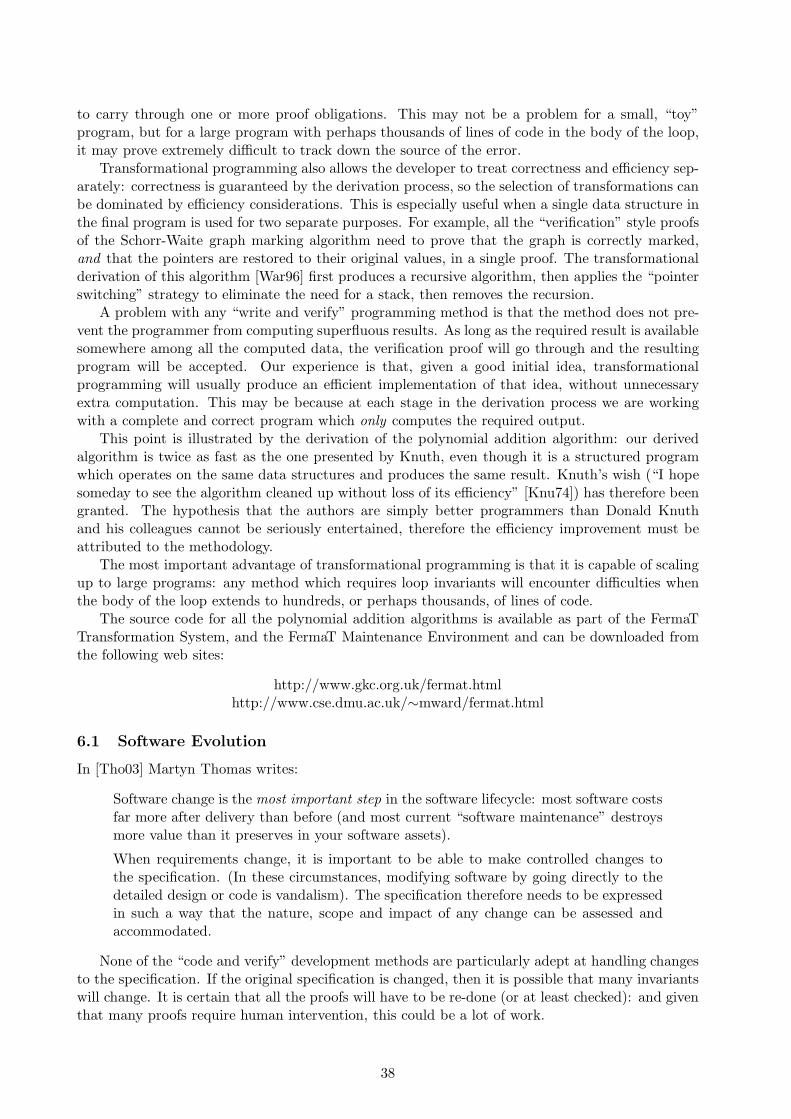
to carry through one or more proof obligations. This may not be a problem for a small, “toy”program, but for a large program with perhaps thousands of lines of code in the body of the loop,it may prove extremely difficult to track down the source of the error.

Transformational programming also allows the developer to treat correctness and efficiency sep-arately: correctness is guaranteed by the derivation process, so the selection of transformations canbe dominated by efficiency considerations. This is especially useful when a single data structure inthe final program is used for two separate purposes. For example, all the “verification” style proofsof the Schorr-Waite graph marking algorithm need to prove that the graph is correctly marked,and that the pointers are restored to their original values, in a single proof. The transformationalderivation of this algorithm [War96] first produces a recursive algorithm, then applies the “pointerswitching” strategy to eliminate the need for a stack, then removes the recursion.

A problem with any “write and verify” programming method is that the method does not pre-vent the programmer from computing superfluous results. As long as the required result is availablesomewhere among all the computed data, the verification proof will go through and the resultingprogram will be accepted. Our experience is that, given a good initial idea, transformationalprogramming will usually produce an efficient implementation of that idea, without unnecessaryextra computation. This may be because at each stage in the derivation process we are workingwith a complete and correct program which only computes the required output.

This point is illustrated by the derivation of the polynomial addition algorithm: our derivedalgorithm is twice as fast as the one presented by Knuth, even though it is a structured programwhich operates on the same data structures and produces the same result. Knuth’s wish (“I hopesomeday to see the algorithm cleaned up without loss of its efficiency” [Knu74]) has therefore beengranted. The hypothesis that the authors are simply better programmers than Donald Knuthand his colleagues cannot be seriously entertained, therefore the efficiency improvement must beattributed to the methodology.

The most important advantage of transformational programming is that it is capable of scalingup to large programs: any method which requires loop invariants will encounter difficulties whenthe body of the loop extends to hundreds, or perhaps thousands, of lines of code.

The source code for all the polynomial addition algorithms is available as part of the FermaTTransformation System, and the FermaT Maintenance Environment and can be downloaded fromthe following web sites:

http://www.gkc.org.uk/fermat.htmlhttp://www.cse.dmu.ac.uk/∼mward/fermat.html

6.1 Software Evolution

In [Tho03] Martyn Thomas writes:

Software change is the most important step in the software lifecycle: most software costsfar more after delivery than before (and most current “software maintenance” destroysmore value than it preserves in your software assets).

When requirements change, it is important to be able to make controlled changes tothe specification. (In these circumstances, modifying software by going directly to thedetailed design or code is vandalism). The specification therefore needs to be expressedin such a way that the nature, scope and impact of any change can be assessed andaccommodated.

None of the “code and verify” development methods are particularly adept at handling changesto the specification. If the original specification is changed, then it is possible that many invariantswill change. It is certain that all the proofs will have to be re-done (or at least checked): and giventhat many proofs require human intervention, this could be a lot of work.

38

With the transformational programming approach, it is likely that many of the informal ideasare still valid for the new specification, and therefore that much of the basic transformation sequencegenerated by these ideas can still be applied to the new specification (generating modified code ateach stage).

One example, which actually involves a small but significant change to the specification, isthe development of the polynomial multiplication algorithm. The change in the specificationsimply involves replacing “+” with “∗”, and adding a new variable for the result — but thisis quite a significant change! However, many of the implementation ideas and transformationsub-sequences used in the derivation of the addition program could also be used in the derivationof the multiplication program: so that, even though the final multiplication algorithm is much morecomplex than the addition algorithm, it took significantly less time to develop.

It would appear that with a properly-written specification (see Section 1.2), a small change to therequirements is likely to result in a small change to the specification. Any informal implementationideas may still be valid: in which case, the derivation process can repeat many of the steps fromthe original derivation. This is because the implementation ideas are used to select the sequence oftransformations to be applied: if the ideas are still valid then it is likely that the sequence is stillvalid and can be applied to the modified specification with only minimal changes. This process canbe streamlined even further with the aid of suitable tool support, such as the FermaT MaintenanceEnvironment.

In order to accommodate future changes to the specification or implementation environment(and to support software evolution in general) it is recommended that the original formal specifi-cation and development history be recorded and maintained: not just the final code. With propertools, there is no need to keep a copy of the final code: since it can be reconstructed automaticallyfrom the specification and development history.

This idea is a natural extension of the current practice with high level language compilers: no-body would dream of compiling a program and then throwing away the source code and maintainingthe generated object code!

References

[06] ISO JTC 1/SC 7, “Software Engineering – Software Life Cycle Processes – Maintenance,”ISO/IEC 14764:2006, 2006.

[ABH06] Jean-raymond Abrial, Michael Butler, Stefan Hallerstede & Laurent Voisin, “An openextensible tool environment for Event-B,” ICFEM , New York–Heidelberg–Berlin (2006).

[Bac09] Ralph-Johan Back, “Invariant Based Programming: Basic Approach and TeachingExperiences,” Formal Aspects of Computing 21#3 (May, 2009), 227–244.

[Bau79] F. L. Bauer, “Program Development By Stepwise Transformations—the Project CIP,” inProgram Construction, G. Goos & H. Hartmanis, eds., Lect. Notes in Comp. Sci. #69,Springer-Verlag, New York–Heidelberg–Berlin, 1979, 237–266.

[BB85] F. L. Bauer, R. Berghammer, et. al. & The CIP Language Group, The Munich Project CIP,Volume I: The Wide Spectrum Language CIP-L, Lect. Notes in Comp. Sci. #183,Springer-Verlag, New York–Heidelberg–Berlin, 1985.

[BMP89] F. L. Bauer, B. Moller, H. Partsch & P. Pepper, “Formal Construction byTransformation—Computer Aided Intuition Guided Programming,” IEEE Trans. SoftwareEng. 15#2 (Feb., 1989).

[BaT87] F. L. Bauer & The CIP System Group, The Munich Project CIP, Volume II: The ProgramTransformation System CIP-S, Lect. Notes in Comp. Sci. #292, Springer-Verlag, NewYork–Heidelberg–Berlin, 1987.

[BiM99] Juan C. Bicarregui & Brian M. Matthews, “Proof and Refutation in Formal SoftwareDevelopment ,” In 3rd Irish Workshop on Formal Software Development (July, 1999).

[BiM96] Richard Bird & Oege de Moor, The Algebra of Programming , Prentice-Hall, Englewood Cliffs,NJ, 1996.

39

[Bro84] M. Broy, “Algebraic Methods for Program Construction: the Project CIP,” in ProgramTransformation and Programming Environments Report on a Workshop directed by F. L.Bauer and H. Remus, P. Pepper, ed., Springer-Verlag, New York–Heidelberg–Berlin, 1984,199–222.

[BGL11] Alan Bundy, Gudmund Grov & Yuhui Lin, “Productive use of failure in top-down formalmethods,” Automated Reasoning Workshop (2011).

[BuD77] R. M. Burstall & J. A. Darlington, “A Transformation System for Developing RecursivePrograms,” J. Assoc. Comput. Mach. 24#1 (Jan., 1977), 44–67.

[But06] Michael Butler, “On the Verified-by-Construction Approach,” BCS FACS, Electronics &Computer Science EPrints Service, 2006, oai:eprints.soton.ac.uk:265110.

[Dar78] J. Darlington, “A Synthesis of Several Sort Programs,” Acta Informatica 11#1 (1978), 1–30.

[Dij] E. W. Dijkstra, “A Constructive Approach to the Problem of Program Correctness.,”Technische Hogeschool Eindhoven, EWD209, 〈 http://www.cs.utexas.edu/users/EWD/ewd02xx/EWD209.PDF〉.

[Dij76] E. W. Dijkstra, A Discipline of Programming , Prentice-Hall, Englewood Cliffs, NJ, 1976.

[Dij70] E. W. Dijkstra, “Notes On Structured Programming,” Technische Hogeschool Eindhoven,EWD249, Apr., 1970, 〈http://www.cs.utexas.edu/users/EWD/ewd02xx/EWD249.PDF〉.

[Dij72] E. W. Dijkstra, “The Humble Programmer,” Comm. ACM 15#10 (Oct., 1972), 859–866.

[Gri81] David Gries, The Science of Programming , Springer-Verlag, New York–Heidelberg–Berlin,1981.

[HHJ87] C. A. R. Hoare, I. J. Hayes, H. E. Jifeng, C. C. Morgan, A. W. Roscoe, J. W. Sanders, I. H.Sørensen, J. M. Spivey & B. A. Sufrin, “Laws of Programming,” Comm. ACM 30#8 (Aug.,1987), 672–686.

[JJL91] C. B. Jones, K. D. Jones, P. A. Lindsay & R. Moore, mural: A Formal Development SupportSystem, Springer-Verlag, New York–Heidelberg–Berlin, 1991.

[Knu74] D. E. Knuth, “Structured Programming with the GOTO Statement,” Comput. Surveys 6#4(1974), 261–301.

[Knu68] D. K. Knuth, Fundamental Algorithms, The Art of Computer Programming#1, AddisonWesley, Reading, MA, 1968.

[LPR98] Charles E. Leiserson, Harald Prokop & Keith H. Randall, “Using de Bruijn Sequences toIndex a 1 in a Computer Word,” CiteSeer, 1998, 〈http://citeseerx.ist.psu.edu/viewdoc/summary?doi=10.1.1.37.8562〉.

[Mor94] C. C. Morgan, Programming from Specifications, Prentice-Hall, Englewood Cliffs, NJ, 1994,Second Edition.

[MRG88] C. C. Morgan, K. Robinson & Paul Gardiner, “On the Refinement Calculus,” OxfordUniversity, Technical Monograph PRG-70, Oct., 1988.

[MoV93] C. C. Morgan & T. Vickers, On the Refinement Calculus, Springer-Verlag, NewYork–Heidelberg–Berlin, 1993.

[NHW89] M. Neilson, K. Havelund, K. R. Wagner & E. Saaman, “The RAISE Language, Method andTools,” Formal Aspects of Computing 1 (1989), 85–114 .

[PrW94] H. A. Priestley & M. Ward, “A Multipurpose Backtracking Algorithm,” J. Symb. Comput. 18(1994), 1–40, 〈http://www.cse.dmu.ac.uk/∼mward/martin/papers/backtr-t.ps.gz〉doi:10.1006/jsco.1994.1035.

[Sen90] C. T. Sennett, “Using Refinement to Convince: Lessons Learned from a Case Study,”Refinement Workshop, 8th–11th January, Hursley Park, Winchester (Jan., 1990).

[Tam95] T. Tammet, “Lambda lifting as an optimization for compiling Scheme to C,” ChalmersUniversity of Technology, Department of Computer Sciences, Goteborg, Sweden, 1995, 〈ftp://ftp.cs.chalmers.se/pub/users/tammet/hobbit.ps〉.

[Tho03] Martyn Thomas, “The Modest Software Engineer,” The Sixth International Symposium onAutonomous Decentralized Systems, ISADS (2003).

[War89] M. Ward, “Proving Program Refinements and Transformations,” Oxford University, DPhilThesis, 1989, 〈http://www.cse.dmu.ac.uk/∼mward/martin/thesis〉.

40

[War90] M. Ward, “Derivation of a Sorting Algorithm,” Durham University, Technical Report, 1990,〈http://www.cse.dmu.ac.uk/∼mward/martin/papers/sorting-t.ps.gz〉.

[War94] M. Ward, “Reverse Engineering through Formal Transformation Knuths “PolynomialAddition” Algorithm,” Comput. J. 37#9 (1994), 795–813, 〈http://www.cse.dmu.ac.uk/∼mward/martin/papers/poly-t.ps.gz〉 doi:10.1093/comjnl/37.9.795.

[War96] M. Ward, “Program Analysis by Formal Transformation,” Comput. J. 39#7 (1996), 〈http://www.cse.dmu.ac.uk/∼mward/martin/papers/topsort-t.ps.gz〉 doi:10.1093/comjnl/39.7.598.

[War99a] M. Ward, “Recursion Removal/Introduction by Formal Transformation: An Aid to ProgramDevelopment and Program Comprehension,” Comput. J. 42#8 (1999), 650–673, 〈http://www.cse.dmu.ac.uk/∼mward/martin/papers/recursion-t.ps.gz〉 doi:10.1093/comjnl/42.8.650.

[War99b] M. Ward, “Assembler to C Migration using the FermaT Transformation System,” InternationalConference on Software Maintenance, 30th Aug–3rd Sept 1999, Oxford, England (1999).

[War93] M. Ward, “Abstracting a Specification from Code,” J. Software Maintenance: Research andPractice 5#2 (June, 1993), 101–122, 〈http://www.cse.dmu.ac.uk/∼mward/martin/papers/prog-spec.ps.gz〉.

[War96] M. Ward, “Derivation of Data Intensive Algorithms by Formal Transformation,” IEEE Trans.Software Eng. 22#9 (Sept., 1996), 665–686, 〈http://www.cse.dmu.ac.uk/∼mward/martin/papers/sw-alg.ps.gz〉 doi:doi.ieeecomputersociety.org/10.1109/32.541437.

[War01] Martin Ward, “The FermaT Assembler Re-engineering Workbench,” International Conferenceon Software Maintenance (ICSM), 6th–9th November 2001, Florence, Italy (2001).

[War04] Martin Ward, “Pigs from Sausages? Reengineering from Assembler to C via FermaTTransformations,” Science of Computer Programming, Special Issue on ProgramTransformation52#1–3 (2004), 213–255, 〈http://www.cse.dmu.ac.uk/∼mward/martin/papers/migration-t.ps.gz〉 doi:dx.doi.org/10.1016/j.scico.2004.03.007.

[WaZ05] Martin Ward & Hussein Zedan, “MetaWSL and Meta-Transformations in the FermaTTransformation System,” 29th Annual International Computer Software and ApplicationsConference, Edinburgh, UK, November 2005 (2005).

[WaZ07] Martin Ward & Hussein Zedan, “Slicing as a Program Transformation,” Trans. ProgrammingLang. and Syst. 29#2 (Apr., 2007), 1–52, 〈http://www.cse.dmu.ac.uk/∼mward/martin/papers/slicing-t.ps.gz〉 doi:doi.acm.org/10.1145/1216374.1216375.

[WaZ10] Martin Ward & Hussein Zedan, “Deriving a Slicing Algorithm via FermaT Transformations,”IEEE Trans. Software Eng., IEEE computer Society Digital Library (Jan., 2010), 〈http://www.cse.dmu.ac.uk/∼mward/martin/papers/derivation2-a4-t.pdf〉doi:doi.ieeecomputersociety.org/10.1109/TSE.2010.13.

[WZH04] Martin Ward, Hussein Zedan & Tim Hardcastle, “Legacy Assembler Reengineering andMigration,” 20th IEEE International Conference on Software Maintenance, 11th-17th SeptChicago Illinois, USA. (2004).

[WZL08] Martin Ward, Hussein Zedan, Matthias Ladkau & Stefan Natelberg, “Conditioned SemanticSlicing for Abstraction; Industrial Experiment,” Software Practice and Experience 38#12(Oct., 2008), 1273–1304, 〈http://www.cse.dmu.ac.uk/∼mward/martin/papers/slicing-paper-final.pdf〉 doi:doi.wiley.com/10.1002/spe.869.

[Wir71] N. Wirth, “Program Development by Stepwise Refinement,” Comm. ACM 14#4 (1971),221–227.

[YaW03] H. Yang & M. Ward, Successful Evolution of Software Systems, Artech House, Boston,London, 2003, ISBN-10 1-58053-349-3 ISBN-13 978-1580533492.

[ZMH02a] Xingyuan Zhang, Malcolm Munro, Mark Harman & Lin Hu, “Mechanized OperationalSemantics of WSL,” IEEE International Workshop on Source Code Analysis and Manipulation(SCAM), Los Alamitos, California, USA (2002).

[ZMH02b] Xingyuan Zhang, Malcolm Munro, Mark Harman & Lin Hu, Weakest Precondition for GeneralRecursive Programs Formalized in Coq, Lect. Notes in Comp. Sci., Springer-Verlag, NewYork–Heidelberg–Berlin, 2002, Proceedings of the 15th International Conference on TheoremProving in Higher Order Logics (TPHOLs).

41