DESIGN AND SIMULATION OF A PASSIVE-SCATTERING NOZZLE IN PROTON

BEAM RADIOTHERAPY

A Thesis

by

FADA GUAN

Submitted to the Office of Graduate Studies of Texas A&M University

in partial fulfillment of the requirements for the degree of

MASTER OF SCIENCE

December 2009

Major Subject: Health Physics

DESIGN AND SIMULATION OF A PASSIVE-SCATTERING NOZZLE IN PROTON

BEAM RADIOTHERAPY

A Thesis

by

FADA GUAN

Submitted to the Office of Graduate Studies of Texas A&M University

in partial fulfillment of the requirements for the degree of

MASTER OF SCIENCE

Approved by:

Chair of Committee, John W. Poston, Sr. Committee Members, Leslie A. Braby Michael A. Walker Head of Department, Raymond J. Juzaitis

December 2009

Major Subject: Health Physics

iii

ABSTRACT

Design and Simulation of a Passive-Scattering Nozzle in Proton Beam Radiotherapy.

(December 2009)

Fada Guan, B.E., Tsinghua University, China

Chair of Advisory Committee: Dr. John W. Poston, Sr.

Proton beam radiotherapy is an emerging treatment tool for cancer. Its basic

principle is to use a high-energy proton beam to deposit energy in a tumor to kill the

cancer cells while sparing the surrounding healthy tissues. The therapeutic proton beam

can be either a broad beam or a narrow beam. In this research, we mainly focused on the

design and simulation of the broad beam produced by a passive double-scattering system

in a treatment nozzle.

The NEU codes package is a specialized design tool for a passive double-

scattering system in proton beam radiotherapy. MCNPX is a general-purpose Monte

Carlo radiation transport code. In this research, we used the NEU codes package to

design a passive double-scattering system, and we used MCNPX to simulate the

transport of protons in the nozzle and a water phantom. We used “mcnp_pstudy” script

to create successive input files for different steps in a range modulation wheel for SOBP

to overcome the difficulty that MCNPX cannot be used to simulate dynamic geometries.

We used “merge_mctal” script, “gridconv” code, and “VB script embedded in Excel” to

process the simulation results. We also invoked the plot command of MCNPX to draw

iv

the fluence and dose distributions in the water phantom in the form of two-dimensional

curves or color contour plots.

The simulation results, such as SOBP and transverse dose distribution from

MCNPX are basically consistent with the expected results fulfilling the design aim. We

concluded that NEU is a powerful design tool for a double-scattering system in a proton

therapy nozzle, and MCNPX can be applied successfully in the field of proton beam

radiotherapy.

v

DEDICATION

To my dear wife - Liuyang

No words can express my love and appreciation to her.

vi

ACKNOWLEDGEMENTS

I would like to thank my committee chair, Dr. John W. Poston, Sr. for his patient

guidance in my study and enthusiastic help in my life. I also would like to thank my

committee members Dr. Leslie A. Braby and Dr. Michael A. Walker for their support

and help throughout my study and research.

I want to thank Dr. Reece and Dr. Ford for teaching me about nuclear

instrumentation and internal dosimetry and radiation biology. Thanks go to faculty and

staff in the Department of Nuclear Engineering at Texas A&M University.

I want to thank the author of the NEU code, Dr. Bernard Gottschalk at Harvard

University, and all the members in MCNP and MCNPX development group at Los

Alamos National Laboratory for developing useful design and simulation tools. I thank

Daryl Hawkins for his maintenance of the computation codes on the grove server. I

thank the researchers at M.D. Anderson Cancer Center for their support in this research.

I thank Dr. Harald Paganetti from Massachusetts General Hospital for his excellent

presentation in the topic of proton therapy at Texas A&M University. Without their

cooperation and information, this research could not have been completed.

Very special thanks go to Ruoming Bi and his parents for their help in my life

and Zeyun Wu for his help in my study.

I also want to thank all my teachers, classmates, colleagues and friends.

Finally, thanks go to my family members and parents-in-law for their love and

encouragement.

vii

NOMENCLATURE

2D Two-dimensional

3D Three-dimensional

ASCII American Standard Code for Information Interchange

CATANA Centro di AdroTerapia e Applicazioni Nucleari Avanzate, Italy

CSDA Continuous Slowing-Down Approximation

EGS Electron and Gamma Shower

FLUKA FLUctuating KAscades

FWHM Full-Width at Half Maximum

GEANT4 GEometry ANd Tracks, version 4

GSI Helmholtzzentrum für Schwerionenforschung GmbH, Germany

HCL Harvard Cyclotron Laboratory (1949-2002)

IBA Ion Beam Applications, S.A., Belgium

LANL Los Alamos National Laboratory

LLUMC Loma Linda University Medical Center

MCNP Monte Carlo N-Particles

MCNPX Monte Carlo N-Particles eXtension

MCNP(X) MCNP or MCNPX

MGH Massachusetts General Hospital

NEU Nozzle with Everything Upstream

NIST National Institute of Standards and Technology, Gaithersburg, MD

viii

NPS Number of Particles to be run in MCNP(X)

PHITS Particle and Heavy Ion Transport code System

PSI Paul Scherrer Institute, Villigen, Switzerland

rms root mean square

SOBP Spread-Out Bragg Peak

SSD Source Surface Distance

VB Visual Basic

ix

TABLE OF CONTENTS

Page

ABSTRACT.............................................................................................................. iii

DEDICATION .......................................................................................................... v

ACKNOWLEDGEMENTS ...................................................................................... vi

NOMENCLATURE.................................................................................................. vii

TABLE OF CONTENTS.......................................................................................... ix

LIST OF FIGURES................................................................................................... xii

LIST OF TABLES .................................................................................................... xvii

1. INTRODUCTION................................................................................................ 1

1.1 Overview ................................................................................................. 1

1.2 Scope of This Thesis ............................................................................... 2

2. OVERVIEW OF PROTON BEAM RADIOTHERAPY..................................... 3

2.1 History and Principle of Proton Beam Radiotherapy.............................. 3

2.2 Proton Therapy Facility........................................................................... 6

2.2.1 Layout of a Typical Proton Therapy Facility ................................... 6

2.2.2 Proton Accelerators and Beam Transport System............................ 7

2.2.3 Beam Delivery System..................................................................... 9

2.2.4 Patient Positioning System............................................................... 19

2.3 Biological Effects.................................................................................... 20

2.4 Secondary Radiation ............................................................................... 20

x

Page

3. METHODS AND CODES USED IN DESIGN AND SIMULATION............... 22

3.1 NEU Codes Package ............................................................................... 22

3.2 Monte Carlo Codes.................................................................................. 24

3.3 Other Codes and Scripts.......................................................................... 26

3.3.1 Solution of Dynamic Geometries..................................................... 26

3.3.2 Mcnp_pstudy Script ......................................................................... 27

3.3.2 Merge_mctal Script .......................................................................... 29

3.3.4 VB Scripts Embedded in Excel........................................................ 29

3.4 Systematic Flow of the Application of These Codes .............................. 30

4. DESIGN OF A DOUBLE-SCATTERING SYSTEM ......................................... 31

4.1 Simulation of Pristine Bragg Peak by MCNPX...................................... 31

4.2 Fitting Process of SOBP Data by BPW .................................................. 35

4.3 Design of Double-Scattering System Using NEU .................................. 38

5. MONTE CARLO SIMULATION OF SIMPLIFIED NOZZLE.......................... 50

5.1 MCNPX Input File for a Passive-Scattering Nozzle............................... 50

5.1.1 Geometry Models............................................................................. 51

5.1.2 Proton Beam Source Definition ....................................................... 60

5.1.3 Physics Settings................................................................................ 63

5.1.4 Tally Types....................................................................................... 64

5.1.5 NPS Settings..................................................................................... 65

5.2 Mcnp_pstudy Parameters and Execution ................................................ 65

xi

Page

5.3 Visualization of Models .......................................................................... 66

5.4 Execution of Merge_mctal ...................................................................... 71

5.5 Simulation Results................................................................................... 73

5.5.1 Results No. 1 .................................................................................... 74

5.5.2 Results No. 2 .................................................................................... 77

5.5.3 Results No. 3 .................................................................................... 81

5.5.4 Results No. 4 .................................................................................... 84

5.5.5 Results No. 5 .................................................................................... 90

5.5.6 Results No. 6 .................................................................................... 92

5.5.7 Results No. 7 .................................................................................... 95

5.5.8 Results No. 8 .................................................................................... 97

6. SUMMARY AND FUTURE WORK.................................................................. 100

6.1 Summary ................................................................................................. 100

6.2 Future Work ............................................................................................ 101

REFERENCES.......................................................................................................... 104

APPENDIX A ........................................................................................................... 107

APPENDIX B ........................................................................................................... 109

APPENDIX C ........................................................................................................... 117

VITA ......................................................................................................................... 119

xii

LIST OF FIGURES

Page

Figure 2-1. Depth-dose distribution of a broad proton beam in soft tissue........................4

Figure 2-2. The formation of a spread-out Bragg peak......................................................4

Figure 2-3. A comparison of depth-dose distributions between photons and protons.......5

Figure 2-4. A typical layout of proton therapy facility ......................................................6

Figure 2-5. Proton therapy facility layout at MGH............................................................7

Figure 2-6. CSDA ranges of protons in water, adipose and bone......................................8

Figure 2-7. An IBA isochronous cyclotron........................................................................9

Figure 2-8. A horizontal beam at CATANA, Italy ..........................................................11

Figure 2-9. IBA gantry system at MGH...........................................................................11

Figure 2-10. PSI gantry in Switzerland............................................................................12

Figure 2-11. A schematic figure of a scanning beam.......................................................13

Figure 2-12. Schematic diagram of a passive-scattering nozzle at LLUMC ...................14

Figure 2-13. Three types of range modulation wheels.....................................................16

Figure 2-14. A final aperture and a patient-specific range compensator .........................17

Figure 2-15. Formation of the conformal dose by a passive-scattering method ..............17

Figure 2-16. The delivery process of a broad beam.........................................................18

Figure 2-17. A scanning pencil beam...............................................................................18

Figure 2-18. Patient positioning system...........................................................................19

Figure 2-19. Mass stopping power of protons in lead......................................................21

Figure 3-1. The structure of the BGware directory..........................................................23

xiii

Page

Figure 3-2. Modification of the “mcnp_pstudy” script ....................................................28

Figure 3-3. Flow chart of the application of codes ..........................................................30

Figure 4-1. The tracks of 250 MeV broad-beam protons.................................................33

Figure 4-2. Depth-dose curves for broad-beam protons ..................................................34

Figure 4-3. Snapshot of “bpw.inp”...................................................................................35

Figure 4-4. Execution of the BPW code ..........................................................................36

Figure 4-5. The fitted Bragg curve for 250 MeV protons................................................37

Figure 4-6. Snapshot of “MDA250.BPK” .......................................................................37

Figure 4-7. A simplified schematic of the NEU design ...................................................40

Figure 4-8. Various quantities on a SOBP curve .............................................................43

Figure 4-9. Contents of “neu.inp” for NEU-Case 1 .........................................................44

Figure 4-10. Contents of “BEAMPICT.INP” for NEU-Case 1 .......................................45

Figure 4-11. Output plots of “neu.inp” for NEU-Case 1 .................................................46

Figure 4-12. Output plot of “BEAMLINE.INP” for NEU-Case 1...................................47

Figure 4-13. Cross-section of lead part in S2 for NEU-Case 1........................................48

Figure 4-14. Comparison of transverse doses from different scattering strengths of S1 .49

Figure 5-1. Illustration of the geometry for a rectangular mesh tally ..............................56

Figure 5-2. Fixed-Y layer for depth-dose and transverse dose ........................................57

Figure 5-3. Fixed-X layer for transverse dose..................................................................57

Figure 5-4. Planes to show dose or fluence distribution ..................................................58

Figure 5-5. The spatial and energy distribution functions in MCNPX ............................61

xiv

Page

Figure 5-6. The spatial Gaussian distribution of proton source on Y-Z plane.................62

Figure 5-7. The energy Gaussian distribution (250 MeV) ...............................................62

Figure 5-8. 3D model of a passive-scattering nozzle in MCNPX-Case 7........................67

Figure 5-9. Schematic of one step on S1..........................................................................67

Figure 5-10. Schematic of a contour-shaped S2 ..............................................................68

Figure 5-11. Schematic of collimator and range shifter...................................................68

Figure 5-12. Schematic of final aperture and patient-specific range compensator..........69

Figure 5-13. Nozzle geometry and proton tracks in MCNPX-Case 1 .............................70

Figure 5-14. Nozzle geometry and proton tracks in MCNPX-Case 4 .............................70

Figure 5-15. Nozzle geometry and proton tracks in MCNPX-Case 7 .............................71

Figure 5-16. Contour depth-dose distribution on the central layer ..................................74

Figure 5-17. Contour transverse dose distribution at the depth of 5 cm ..........................75

Figure 5-18. The depth-dose distribution along the central axis (X-axis) .......................76

Figure 5-19. The transverse dose distribution at the depth of 7.6 cm along the Y-axis...77

Figure 5-20. Geometry and tracks of protons scattered by a scattering foil ....................78

Figure 5-21. The contour transverse dose distribution for Results No. 2 ........................78

Figure 5-22. The contour transverse dose distribution for Results No. 2 in 2D mode ....79

Figure 5-23. The contour transverse dose distribution for Results No. 2 in 3D mode ....79

Figure 5-24. The transverse dose along the Y-axis for Results No. 2..............................80

Figure 5-25. Geometry and tracks of protons scattered by a scattering foil and S2 ........81

Figure 5-26. The contour transverse dose distribution for Results No. 3 ........................82

xv

Page

Figure 5-27. The transverse dose along the Y-axis for Results No. 3..............................83

Figure 5-28. The energy spectrum of incident protons in water phantom .......................85

Figure 5-29. The angular distribution spectrum of incident protons in water phantom...86

Figure 5-30. The depth-dose and transverse dose distributions for Results No. 4...........87

Figure 5-31. The contour depth-dose distribution in the central layer for Results No. 4 88

Figure 5-32. The formation of the SOBP by weighted pristine peaks .............................89

Figure 5-33. The comparison of SOBP between NEU and MCNPX results...................89

Figure 5-34. The depth-fluence distribution along X-axis...............................................90

Figure 5-35. The depth-dose and transverse dose distributions for Results No. 5...........91

Figure 5-36. The contour dose distributions for Results No. 5 ........................................92

Figure 5-37. The depth-dose distribution for Results No. 6.............................................93

Figure 5-38. The contour depth-dose distribution for Results No. 6 ...............................94

Figure 5-39. The contour transverse dose distributions at different depths .....................95

Figure 5-40. The dose distributions in the central layer plotted by Excel .......................96

Figure 5-41. The relative errors for dose distributions in the central layer......................96

Figure 5-42. The depth-dose distributions in the central layer plotted by MCNPX ........97

Figure 5-43. The depth-dose distribution for Results No. 8.............................................98

Figure 5-44. The contour transverse dose distribution for Results No. 8 ........................99

Figure A-1. Results from NEU-Case 5 (180 MeV, medium field) ................................107

Figure A-2. Results from NEU-Case 9 (100 MeV, small field) ....................................108

Figure B-1. Command to execute the “mcnp_pstudy” script.........................................113

xvi

Page

Figure B-2. Creation of sub-directories and files by the “mcnp_pstudy” script ............114

Figure B-3. The content of “mergecsh” .........................................................................114

Figure B-4. The modifications of the “mctal” files from MCNPX-Case 1....................115

Figure B-5. The execution and print-out information from “mergecsh” .......................116

xvii

LIST OF TABLES

Page

Table 3-1. The list of files or codes in the BGware directory..........................................24

Table 3-2. Guidelines for interpreting the relative error Ra .............................................26

Table 4-1. The Bragg peak position and range in water phantom ...................................34

Table 4-2. Parameters modified in “bpw.inp”..................................................................36

Table 4-3. Materials used in NEU design ........................................................................40

Table 4-4. Expected SOBP width ....................................................................................41

Table 4-5. Uncollimated field sizes..................................................................................41

Table 4-6. NEU-Case No. for different settings...............................................................42

Table 4-7. The final parameters for 9 NEU cases ............................................................48

Table 5-1. Contents in an MCNPX input file for a passive nozzle..................................50

Table 5-2. Components used in a typical passive-scattering-nozzle problem .................52

Table 5-3. Composition of materials and CSDA ranges of 250 MeV protons ................52

Table 5-4. Components-in-nozzle conditions in a nozzle for MCNPX ...........................53

Table 5-5. Parameters for different field sizes .................................................................53

Table 5-6. Tally-geometry conditions..............................................................................55

Table 5-7. Parameters for mesh tally by collimated beams .............................................56

Table 5-8. Cases simulated by MCNPX ..........................................................................59

Table 5-9. Parameters of S1 and S2 from NEU-Case 1 ...................................................60

Table 5-10. Parameters for energy Gaussian distributions ..............................................61

Table C-1. Coordinate or Index of i in the mesh tally for transverse dose distribution.118

1

1. INTRODUCTION

1.1 Overview

Currently, cancer is one of the most threatening diseases for humans and other

beings. Scientists worldwide are trying to find more effective methods to conquer this

disease. The current cancer therapy methods mainly include surgery, chemotherapy,

radiotherapy or a combination of these (Bayle and Levin 2008). A little over 50% of all

cancer patients will require radiotherapy at some time during their illness. The basic

principle is to use ionizing radiation (internal or/and external) to deposit energy in a

tumor to kill the cancer cells. In this thesis, we will introduce an emerging radiation

treatment tool - proton beam radiotherapy, which is called “the state of the art” technique

in radiation therapy (Paganetti and Bortfeld 2005).

The purpose of radiation therapy is to maximize the dose delivered to the tumor

region while minimizing the dose to the surrounding healthy tissues or organs (Weber

2006). The optimized result from radiation therapy is that the profile of the spatial

distribution of absorbed dose is exactly the same as the profile of the tumor volume.

Although it is not so easy to obtain this optimized result, some techniques can be used to

achieve it. Conformal techniques have been and are being developed to achieve this aim

(Paganetti and Bortfeld 2005). “Conformal” means the shape or profile of the high dose

region is the same as the tumor region, while low-dose or non-dose regions cover the

____________ This thesis follows the style of Health Physics.

2

surrounding healthy tissues or organs. The depth-dose distributions for high-energy

protons make it possible for this radiation to offer a high degree of conformity to the

tumor volume. This is one important reason proton therapy techniques are increasingly

popular in clinical applications.

1.2 Scope of This Thesis

In this thesis, we will provide a detailed design and simulation procedure of a

passive-scattering nozzle in proton beam radiotherapy.

Section 2 will provide an overview of proton beam therapy, including the history,

basic principles, facilities, and some considerations about this treatment method.

Section 3 will introduce the design and simulation codes and several other scripts

used in this research.

Section 4 will provide a detailed design procedure of a double-scattering system.

The design results will be used in Section 5.

Section 5 will provide a detailed Monte Carlo simulation procedure of a passive-

scattering nozzle to verify the design results from Section 4 and obtain the dose and

fluence distributions. The geometric models, particle tracks, and simulation results will

be shown graphically.

Section 6 will summarize this research and point out the uncompleted tasks and

future work.

3

2. OVERVIEW OF PROTON BEAM RADIOTHERAPY

2.1 History and Principle of Proton Beam Radiotherapy

In 1946, Robert R. Wilson (Wilson 1946) first proposed the use of protons for

radiation therapy, at Harvard Cyclotron Laboratory (HCL). In 1954, the first patient was

treated at Lawrence Berkeley Laboratory. By December, 2007, thirty-three proton

therapy centers had been established worldwide, and twenty-six of them are still active.

Seven future proton therapy facilities are currently under construction or are fully funded.

From 1954 to 2007, 53,439 patients had received proton therapy (ICRU 2007).

Proton therapy is a tool to treat cancer. It uses the ionizing ability of protons to

damage the DNA of the cancer cells. Like other forms of radiotherapy, proton therapy

works by aiming energetic ionizing particles onto the target tumor.

The physical rationale of proton therapy is based on the well-defined penetration

range of protons. In the depth-dose curve, a dose peak (called the “Bragg peak”) occurs

at the end of range, shown in Figure 2-1. If a tumor is located at the Bragg peak, it can

obtain the highest dose from the radiation. Since a tumor is not a point but rather a

volume, a single Bragg Peak cannot cover the whole tumor. If several Bragg peaks from

protons with different ranges are superimposed properly to form a wide dose peak, the

target tumor can be covered longitudinally. This wide dose peak is called a “Spread-Out

Bragg Peak” (SOBP), shown in Figure 2-2. The incident proton beam can form an SOBP

4

by sequentially penetrating absorbers with different thickness, e.g., via a range

modulator or ridge filters (Chu et al. 1993).

Figure 2-1. Depth-dose distribution of a broad proton beam in soft tissue

Figure 2-2. The formation of a spread-out Bragg peak

(ICRU 2007)

5

The clinical rationale of proton therapy is the feasibility of delivering higher dose

to the tumor, leading to an increased tumor control probability (Paganetti and Bortfeld

2005). The physician can choose the energy and intensity of proton beam according to

the position and profile of the tumor. Compared with traditional photon therapy, proton

therapy has many advantages, e.g., good high-dose conformity to tumor and lower dose

to healthy tissue, lower tumor reoccurrence rate, and fewer adverse side effects, etc.

(Olsen et al. 2007). Proton therapy is a preferred treatment method for pediatric cancers

because it will not affect the growth of the young patients. A comparison of dose

distributions between photons and protons is shown in Figure 2-3.

Figure 2-3. A comparison of depth-dose distributions between photons and protons

(Weber 2006)

6

2.2 Proton Therapy Facility

2.2.1 Layout of a Typical Proton Therapy Facility

A typical proton-therapy facility includes three main components: an accelerator

with energy selection system, a beam transport system, and a treatment delivery system.

An illustration of a typical proton-therapy facility is shown in Figure 2-4, and the layout

of proton-therapy facility at Massachusetts General Hospital (MGH) is shown in Figure

2-5.

Figure 2-4. A typical layout of proton therapy facility

(The National Association for Proton Therapy 2009)

7

Figure 2-5. Proton therapy facility layout at MGH

(ICRU 2007)

2.2.2 Proton Accelerators and Beam Transport System

Accelerators are used to produce the treatment proton beams with the energy

high enough to reach the deepest position of the tumors. According to the range (Berger

et al. 2005) chart shown in Figure 2-6, the energy of 215 MeV is required for incident

protons to achieve the depth of 30 g cm-2 in the body. The protons can lose some energy

in the beam-modifying components, so the emerging energy of protons from an

accelerator should be a little higher, i.e., 225 to 250 MeV. In addition, the beam intensity

must be high enough to deliver the required therapeutic doses to the tumor within a

reasonable time. If the required dose rate delivered uniformly to a one liter target tumor

is 2 Gy per minute, the typical beam intensities should be in the range of 1.8×1011 to

8

3.6×1011 particles per minute. The exact energy and intensity requirements are

dependent on the beam delivery mode (either scattering or scanning) actually used in

therapy (ICRU 2007).

Figure 2-6. CSDA ranges of protons in water, adipose and bone

The types of accelerators that can be used to produce energetic protons include

linear accelerators, classical cyclotrons, isochronous cyclotrons, synchrocyclotrons or

synchrotrons. At present, only cyclotrons and synchrotrons are used in dedicated

hospital-based, proton-therapy facilities. The mechanisms of different accelerators

9

related to proton therapy can be found in ICRU Publication 78 (2007). One cyclotron

designed by Ion Beam Applications, S.A. (IBA) is shown in Figure 2-7.

Figure 2-7. An IBA isochronous cyclotron

(Medical Physics Web 2009)

The beam transport system is actually the connection part between the

accelerators and treatment rooms. It is used to transfer the beam from the outlet of the

accelerator to the entrance of the treatment rooms. A series of magnets are used to bend,

steer and focus the beam in the beam transport line.

2.2.3 Beam Delivery System

A beam delivery system can comprise several subsystems and may include some

or all of the following: a gantry, a beam nozzle (equipped with a snout), a volume-

10

tracking and beam-gating device, and a patient-positioning and immobilization system.

The beam delivery system is enclosed in a treatment room to separate the accelerator and

beam line. This protects the patients and allows personnel to move freely between

treatment rooms while the beam is in use within adjacent restricted areas (ICRU 2007).

According to the alignment of the treatment head (also called “nozzle”) in the

treatment rooms, the beam delivery systems are categorized into two types: a gantry

system or a stationary beam delivery system, previously shown in Figure 2-4 and Figure

2-5. A fixed horizontal beam (stationary beam) can only be used to treat patients in a

seated or near-seated position, e.g., a patient with an ocular tumor or tumor of the skull.

Figure 2-8 shows a fixed horizontal beam delivery device at Centro di AdroTerapia e

Applicazioni Nucleari Avanzate(CATANA), Italy. To irradiate a patient from any

desired angle, the gantry system is introduced. A gantry equipped with a treatment head

can rotate around the patient lying on a movable table. The nozzle delivers the beam to

the patient at the desired angle. Two typical gantries are shown in Figure 2-9 and Figure

2-10. One is the IBA gantry at MGH, and the other is the gantry used at Paul Scherrer

Institute (PSI) in Switzerland. Please notice that the bending paths for protons and

isocenters are different in these two gantries.

11

Figure 2-8. A horizontal beam at CATANA, Italy

(Proton Therapy Room 2008)

Figure 2-9. IBA gantry system at MGH

(Lawrence Berkeley National Laboratory 2009; Paganetti and Bortfeld 2005)

12

Figure 2-10. PSI gantry in Switzerland

(PSI Proton Therapy Facility 2009)

To spread out the beam laterally, the beam-delivery techniques are categorized

into two types: dynamic scanning or passive scattering (ICRU 2007). The dynamic

scanning technique is a time-dependent method to deliver the desired dose to the target

tumor in a scanning mode. In a passive scattering nozzle, a narrow beam is scattered by

a scattering system to form a broad beam laterally.

In some dynamic scanning modes, the direction and path of a narrow beam

(pencil beam) is controlled by magnets in order to scan the target tumor in a zigzag route

laterally and layer by layer longitudinally. This working mode is also called “active

scanning”, which looks like a painting procedure. Pencil beam scanning is an Intensity

13

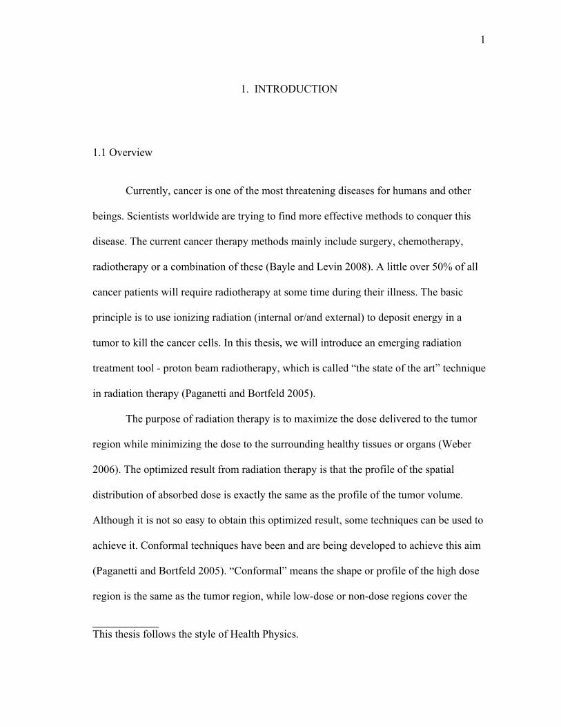
Modulated Proton Therapy (IMPT) technique. A scanning beam is composed of a

number of finite pencil beams. The schematic of an active scanning beam is shown in

Figure 2-11. A broad beam (with a Gaussian lateral profile) can also be used as a

scanning beam. This method is usually called “uniform scanning”, which is only used

for the delivery of uniform-intensity dose distributions. It needs wobbling magnets to

move the beam; besides, it also needs a scatterer, patient collimators and a compensator.

Figure 2-11. A schematic figure of a scanning beam

(GSI Heavy Ion Research Center 2008)

The design and simulation of a passive-scattering nozzle is the topic of this

research. We will discuss it in detail. A passive-scattering nozzle used at Loma Linda

University Medical Center (LLUMC) is shown in Figure 2-12 (ICRU 2007).

14

Figure 2-12. Schematic diagram of a passive-scattering nozzle at LLUMC

(ICRU 2007)

The main components of a passive-scattering nozzle include some or all of the

following: a vacuum chamber, a first scatterer, a range modulation wheel or ridge filters,

a second scatterer, several collimators, a final aperture, a patient-specific range

compensator, beam profile monitors, ion chambers, and a set of range shifters.

The function of scattering system is to broaden the narrow beam to form a flat

transverse dose distribution to cover the tumor laterally. The function of a range

modulation wheel or ridge filters is to modulate the beam to form a SOBP depth-dose

15

distribution to cover the tumor longitudinally. The combination of a scattering system

and a range modulator (wheel or filters) make it possible to form a high-dose region to

cover the tumor region fully.

The other devices, including collimators, a final aperture and a patient-specific

compensator, and range shifters are used to spread and limit the beam profile to make

the high dose distribution region “conformal” to the tumor region. All efforts are made

to achieve one purpose: maximizing the dose in the target tumor and sparing the

surrounding healthy tissues. However, even though there is a very sharp distal drop in

depth-dose distribution, the healthy tissues proximal to the target are still exposed to

very high doses, which can be seen from the SOBP curve discussed later. Scattering

theory will be discussed in Section 4 and a simplified passive-scattering nozzle will be

modeled in Section 5.

Figure 2-13 shows several different range modulation wheels. The common

materials used in range modulation wheel can be plastic or aluminum alloy, depending

on the therapeutic requirements. These common plastic materials include poly methyl

methacrylate (PMMA), acrylonitrile butadiene styrene (ABS) resin and Lexan. Figure 2-

14 shows a final aperture (brass) and a patient-specific range compensator (acrylic).

Figure 2-15 shows the schematic of the formation of the “conformal” dose distribution in

a passive-scattering treatment method.

16

Figure 2-13. Three types of range modulation wheels

(Paganetti and Bortfeld 2005; Proton Therapy Room 2008; Free Patents Online 2009)

17

Figure 2-14. A final aperture and a patient-specific range compensator

(Gottschalk 2009)

Figure 2-15. Formation of the conformal dose by a passive-scattering method

(Advanced Cancer Therapy 2009)

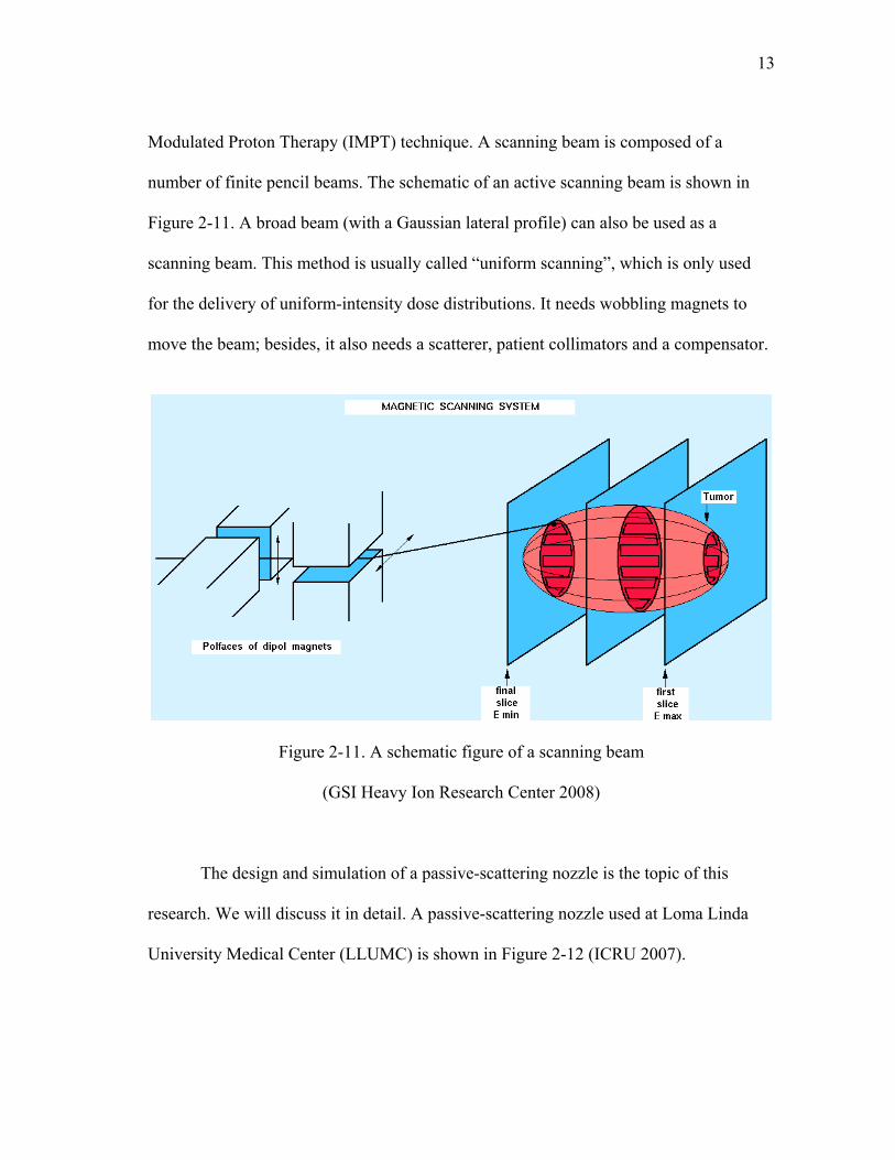
The examples of a broad beam and a pencil beam used at M.D. Anderson Cancer

Center are shown in Figures 2-16 and 2-17. Figure 2-16.a shows the procedure how a

18

narrow beam passes through a rotating range modulation wheel; Figure 2-16.b shows

how the scattered broad beam is shaped to the profile of the tumor; Figure 2-16.c shows

how this “conformal” beam is aimed to the target tumor. Figure 2-17 shows the

procedure that a pencil beam is “painting” on the tumor “actively”.

a b c

Figure 2-16. The delivery process of a broad beam

(Proton Therapy Center at M.D. Anderson Cancer Center 2008)

Figure 2-17. A scanning pencil beam

(Proton Therapy Center at M.D. Anderson Cancer Center 2008)

19

2.2.4 Patient Positioning System

Proton therapy is also a type of target-conformal technique (Paganetti and

Bortfeld 2005). Patient positioning is very critical in the whole treatment procedure,

which can affect the decision of treatment plan and the treatment effect. The tumor

position and its surrounding structures, especially bones, on the treatment day should be

identical to the position on the positioning day. Several factors can affect the result of

the treatment. For example, if bone is suddenly moved into the beam on the treatment

day, the high dose region will shift backwards, which will decrease the effect of the

treatment. The physiologic motion of organs can also affect the therapy. For example, in

the treatment of lung tumors, the dose will be disturbed due to the motion of lungs.

The schematic of patient positioning system (PPS) are shown in Figure 2-18

(Meggiolaro et al. 2004).

Figure 2-18. Patient positioning system

(Meggiolaro et al. 2004)

20

2.3 Biological Effects

The relative biological effectiveness (RBE) of protons is defined as the ratio of

the absorbed dose from the reference radiation (photons) and the absorbed dose from

protons producing the same biological effect. There are no proton RBE values based on

human tissue response data, and there are no experimental data from in vivo systems

supporting the specific RBE. Clinically, a generic RBE value of 1.1 is applied to all

tissues in the direct proton beam path (ICRU 78 2007).

More information about the biological effects of proton beams in the therapeutic

energy range can be found in ICRU Publication 78 (2007). Paganetti and Bortfeld (2005)

also provided a systematic review on the biological effects.

2.4 Secondary Radiation

When protons pass through matter, they will slow down by interacting with the

matter by Coulomb interactions and nuclear interactions (Paganetti and Bortfeld 2005).

The secondary radiation, such as secondary neutrons and recoil nuclei, will be produced

by nuclear interactions. Shielding for neutrons is necessary for any proton therapy

facility. The production of neutrons cannot be avoided. Shielding can be used to reduce

the effect of neutrons produced in the scattering system, the aperture and the

compensator, but nothing can be done to avoid the neutrons produced in the patient’s

body (Paganetti and Bortfeld 2005).

21

The mass stopping power of protons in lead (Berger et al. 2005) is shown in

Figure 2-19. The nuclear stopping power is much less than the electronic stopping power.

Hence, we simplify the problem by omitting the production of neutrons and recoil nuclei.

The purpose is to record the contribution from incident protons and secondary radiation

separately. The effect of secondary radiation will be considered in future research.

Figure 2-19. Mass stopping power of protons in lead

(Berger et al. 2005)

22

3. METHODS AND CODES USED IN DESIGN AND SIMULATION

In this Section, we will introduce a specialized design tool for a double-scattering

system in a passive-scattering nozzle. We also will introduce some Monte Carlo particle

transport codes. Finally, we will provide a method using static geometries to obtain

simulation results for dynamic geometries. This is the most valuable part of this research.

This method was realized by executing several auxiliary codes or scripts.

3.1 NEU Codes Package

The NEU codes package is a specialized tool kit including several subroutines

for designing the double-scattering system in a passive-scattering proton nozzle. NEU

means “Nozzle with Everything Upstream,” which is also the design principle for a

passive-scattering nozzle. Firstly, NEU was written by Bernard Gottschalk in

FORTRAN language at HCL in the late 1980’s. During the next few years the program

and designs were furnished to a number of proton therapy centers. NEU was tested at

HCL and used to design the standard IBA nozzle and components for M.D. Anderson

Cancer Center. Currently it is still very useful for the design and improvement of proton

therapy nozzles.

The compressed package of NEU (named “BGware.zip”) can be obtained from

Dr. Gottschalk’s website. NEU can be run on a Windows XP operating system. The

23

structure of the “BGware” directory is shown in Figure 3-1, and the contents are listed in

Table 3-1.

We mainly used the files or codes in subdirectories “bpw”, “data”, “execs”, and

“neu.” All the executable files, such as “bpw.exe” and “neu.exe,” are contained in the

directory of “execs.” Input files and output files related with “neu.exe” are located in the

directory of “neu.” The files related to “bpw.exe” are contained in the “bpw” directory.

The fitted Bragg peak data files (*.bpk) created by “bpw.exe” are copied from the

directory of “bpw” to “data.” These *.bpk files will be invoked by “neu.exe.” More

detailed information can be found in NEU User Guide (Gottschalk 2006). The function

and application of each code will be described in Section 4 with examples.

Figure 3-1. The structure of the BGware directory

24

Table 3-1. The list of files or codes in the BGware directory

Sub-directory Description File type or name Original Bragg peak data *.txt; *.dat; *.psi; *.scx Input files for bpw.exe bpw.inp Fitted Bragg peak data *.bpk

bpw

Other output files *.bmp Range-energy table *.ret data Fitted Bragg peak data *.bpk (copied from bpw directory)

execs Executable files

Bpw.exe; CPO2.exe; FitDD.exe; fitscan.exe; laminate.exe; lookup.exe; neu.exe; scanfor.exe

Catalog of NEU runs NEU.CAT Input files for neu.exe Neu.inp Beam line picture input file BEAMPICT.INP

neu

Output files *.mod; *.con; *.axd; *.axh; *.bmp; *.out; *.log; SOBP.DAT

3.2 Monte Carlo Codes

The Monte Carlo (MC) method was first used in the 1940s by physicists working

on nuclear weapon projects at the Los Alamos National Laboratory (LANL). It is a

random sampling computational algorithm (Wikipedia 2008). It is not limited by the

dimensions of problems. It tracks the histories of a large number of individual events and

records some aspects according to their average behavior. It has been applied in many

fields, such as high-energy physics, radiation detection, space radiation, medical physics,

and economics. With the computerization spreading, lots of MC codes have been

developed. In the particles transport field, the popular MC codes include, MCNP(X),

EGS, Geant4, Fluka, and PHITS.

25

Monte Carlo dose calculations are known to be more accurate in dosimetry than

commercial treatment planning systems that are based on fast but approximating semi-

empirical algorithms (Mohan and Nahum 1997). Except for EGS, any of the other MC

codes mentioned above can be used in the simulation of proton therapy problems. The

accuracy of MCNPX in predicting dose distributions in proton therapy have been

confirmed by previous investigations (Newhauser et al. 2007), and the benchmarking of

MCNPX applied to the nozzle at M.D. Anderson Cancer Center (Titt et al. 2008). The

MCNPX code was adopted for this research. The other available codes will be applied in

future work.

MCNP and MCNPX were developed by LANL. MCNPX is the extension of

MCNP. MCNP can only be used to track neutrons, photons and electrons (X-5 Monte

Carlo Team 2003), but MCNPX can be used to track nearly all particles at nearly all

energies (Pelowitz 2008). MCNPX utilizes the latest nuclear cross section libraries and

uses physics models for particle types and energies where tabular data are not available.

Several different tally cards can be used to score different physical quantities. The tally

results are tabulated in the pair of “mean and relative error”. The guidelines for

interpreting the relative error in statistics from tallies are shown in Table 3-2.

Visual Editor is a visualization tool for MCNP or MCNPX. It was developed by

Schwarz RA and maintained by Visual Editor Consultants (Schwarz et al. 2008). It

integrates an mcnp5.exe or mcnpx.exe in its kernel. It can be used to aid the user to

create the input files, show the geometry and particles tracks, and plot the cross section

and tally results. The geometry visualization can be in two-dimensional (2D) or three-

26

dimensional (3D) mode, but the particle source and tracks can be shown only in 2D

mode.

In this research, we will also use “gridconv”, a subroutine of MCNPX, to deal

with the data from the mesh tally.

Table 3-2. Guidelines for interpreting the relative error Ra

Range of R Quality of the tally 0.5 to 1.0 Not meaningful 0.2 to 0.5 Factor of a few 0.1 to 0.2 Questionable < 0.10 Generally reliable < 0.05 Generally reliable for point detectors a The guidelines are listed in MCNP5 Manual Volume I (X-5 Monte Carlo Team 2003).

3.3 Other Codes and Scripts

Before we introduce the other codes and scripts, the problem of dynamic

geometries must be discussed.

3.3.1 Solution of Dynamic Geometries

MCNP(X) can be used only to simulate problems with static geometries and

fixed settings for a single problem. The input parameters cannot vary with time.

However, in a real passive-scattering proton therapy problem, in order to realize a SOBP

dose curve, the range modulation wheel is rotating during the whole treatment process. It

seems impossible to simulate the dynamic proton therapy problem using MCNPX. A

common method used to produce a SOBP curve is to use the “Matlab” code to solve a

matrix-equation to obtain a “weighting factor” for each pristine Bragg peak (Oertli 2006),

27

and to use the solution as the probability on the energy spectrum of the source. In this

method, the particles after the range modulation wheel are assumed to be the incident

source particles, because the wheel is not simulated physically. Actually, this method

can be considered only to be an approximate solution, because not all the SOBP matrixes

have rational solutions, and in some cases, the obtained weighting factors are negative.

In this research, if the design parameters are chosen properly, the weighting

factor and thickness of each step in a range modulation wheel can be obtained using

NEU. Hence, it is not necessary to solve a matrix-equation. Assuming that a whole

wheel is modeled in an MCNPX input file, can we make it rotate in the treatment

procedure? The answer is obviously no. We cannot simulate a real rotating wheel using

MCNPX, but we can try some methods to obtain the same results as if the wheel were

“rotating.” Since parameters for each step are known, we can setup a series of input files,

in each of which, only one step is used and the weighting factor of each step is used as

the “weight” of source. After running each problem using MCNPX, we sum the results

from different cases. We can declare that the sum is the same as the result from a

rotating wheel. So, this simulation method can be called “replacing the dynamic by

static.” As to the normalization of the simulation results, we will discuss this topic in

Section 5.

3.3.2 Mcnp_pstudy Script

To create the input files for each step one by one requires a great deal of time. In

order to save time, we used a Perl script “mcnp_pstudy” to set up input files in a batch.

28

This Perl script was developed by Brown et al (2004). It can be used to automate the

setup, execution, and collection of results from a series of MCNP5 Monte Carlo

calculations, each of which must contain varying input specifications. If the setting of

this script is proper, it can also be used to run MCNPX problems, but currently it cannot

be used to collect the mesh tally results from MCNPX. In this research, we used this

script to create a series of input files, each of which contained the parameters from a

single step in a modulation wheel, such as the materials, thicknesses and source weight.

Before using “mcnp_pstudy”, the user should point the “$MCNP” on the 152nd

line to the location of user’s MCNP(X). In some cases, the users should also comment

the 153rd line to run this script correctly. The modification is shown in Figure 3-2.

Figure 3-2. Modification of the “mcnp_pstudy” script

To limit the float number to 4 for a result from an arithmetic expression, a line of

script was added after the 654th line ($val = eval( $expr );) in original “mcnp_pstudy”

script. The added content is “$val = sprintf("%.4f", $val); ,” so that the contents in each

line of the new produced input file will not exceed the limits of the 80th column required

by MCNP(X).

29

3.3.2 Merge_mctal Script

Even though “mcnp_pstudy” cannot be used to collect the mesh tally results from

MCNPX problems, we can solve it by using another Perl script “merge_mctal.” This

script is used to merge and average the tally results and statistical uncertainties. This

script was developed by Brown and Sweezy in 2003 and was updated by Brown in 2004

(Brown 2008). It is designed only for MCNP5 tally results. Because there are some

minor discrepancies (mainly the particle types) in the “mctal” files (tally data file)

between MCNP5 and MCNPX, this script cannot be used to merge “mctal” files from

MCNPX directly, especially for mesh tally results. However, if the mesh tally is

modified to be a “F5” detector tally and the format of particle types is modified, the

“merge_mctal” script can be used to merge the “mctal” files from MCNPX. After the

combination, the “F5” tally in the new combined mctal file should be changed back to

the mesh tally. In other words, first the “mctal” file is changed from MCNPX format to

MCNP5 format; then it is changed back.

3.3.4 VB Scripts Embedded in Excel

Additionally, referring to the VB scripts of output visualization (Schwarz 2007),

we also developed some “VB scripts embedded in Excel” to read in the data from

“mctal” files (in DOS format) from MCNP5 or MCNPX and distribute the data in a

specified order and format. These VB scripts are very convenient for the users to deal

with the data and plot the curves.

30

3.4 Systematic Flow of the Application of These Codes

The systematic flow of the application of all the codes is shown in Figure 3-3.

Chapter 5

Chapter 4

Pristine Bragg Peak by MCNPX

“mcnp_pstudy” to setup cases; MCNPX execution

Visualization by Visual Editor

MCNPX Z to plot 2D curve and color contour

Data processing: gridconv, “merge_mctal”, VB scripts.

Double-scattering system design by NEU

Data fitting by BPW in NEU codes package

Figure 3-3. Flow chart of the application of codes

31

4. DESIGN OF A DOUBLE-SCATTERING SYSTEM

In this section, we will introduce the whole design procedure of a double-

scattering system in a passive-scattering nozzle in proton beam radiotherapy.

The first step is providing measured depth-dose data in a water phantom from a

broad monoenergetic proton beam. In this research, because the clinical measurement

data were not provided, we used the simulated depth-dose data in a water phantom from

MCNPX to replace the measured data.

The second step involves using the BPW code in the NEU codes package to fit

the depth-dose data from MCNPX. These data are read into the NEU code as the

reference data to be used in designing the double-scattering system for a given SOBP

width.

The third step involves using the NEU code to design the double-scattering

system, including a wheel (first scatterers and range modulation steps) and a contour-

shaped scatterer, to meet the requirements in clinical applications.

4.1 Simulation of Pristine Bragg Peak by MCNPX

The NEU code cannot be used to compute the effective stopping power

theoretically, while it deduces it from the user’s measured Bragg-peak data, in which, all

the related effects such as nuclear effects, range straggling, and energy spread about the

user’s facility, are included automatically. This is why the user needs to provide the

32

measured Bragg-peak data first. An MCNPX simulation was used as an “experimental

measurement.”

In this step, the necessary input parameters include the energy, radius and

direction of the incident proton beam, the distance between source and the surface of the

water phantom, and the size of the water phantom.

The synchrotron at M.D. Anderson Cancer Center can provide proton energies

between 100 MeV and 250 MeV. The available eight energy intervals include 100, 120,

140, 160, 180, 200, 225 and 250 MeV (Zheng et al. 2008). The source particles were

limited to a disc with a radius of 10 cm on the Z = -300 cm plane and the emitting

protons were assumed to fly along the Z-axis.

A recommended value of source surface distance (SSD) in ICRU Publication 78

(2007) is 300 cm. We also adopted 300 cm as the SSD in this research.

According to the range of protons in water, shown in Figure 2-6, a 40 cm depth is

enough to stop the 250 MeV protons. In order to capture all the protons, the lateral side

of the water phantom was set to 80 cm. The final size of the water phantom was 80

cm×80 cm×40 cm. The size of each water cell used to score the absorbed dose was 80

cm× 80 cm× 0.1 cm.

We used Visual Editor to check the geometry and the particle tracks. Figure 4-1

shows the tracks of 250 MeV broad-beam protons.

33

Figure 4-1. The tracks of 250 MeV broad-beam protons

The number of particles to be run was set to one million. The simulation results

from MCNPX for 8 energy groups were plotted as depth-dose curves and are shown in

Figure 4-2. Most of the tally results satisfied the statistical requirement shown in Table

3-2. However, several tally regions near the range of protons had higher relative errors

due to the lower-sampling efficiency. The Bragg peak positions for 8 energies in this

experimental setting are listed in Table 4-1. A comparison of projected ranges between

MCNPX and NIST data (Berger et al. 2005) are also listed in this table. The MCNPX

simulation can be accepted because the relative differences are lower than 5%.

In the following research, only 100, 180 and 250 MeV were used as the initial

kinetic energies of the proton beams.

34

Figure 4-2. Depth-dose curves for broad-beam protons

Table 4-1. The Bragg peak position and range in water phantom

Energy (MeV)

Peak position (cm)

Projected range from MCNPX (cm)

Projected range from NIST (cm)

Relative difference (MCNPX-NIST)/NIST

100 7.4 7.9 7.707 2.50 % 120 10.3 10.9 10.65 2.35 % 140 13.6 14.3 13.96 2.44 % 160 17.2 18.2 17.63 3.23 % 180 21.1 22.3 21.63 3.10 % 200 25.4 26.9 25.93 3.74 % 225 31.2 33.1 31.71 4.38 % 250 37.3 39.6 37.90 4.49 %

35

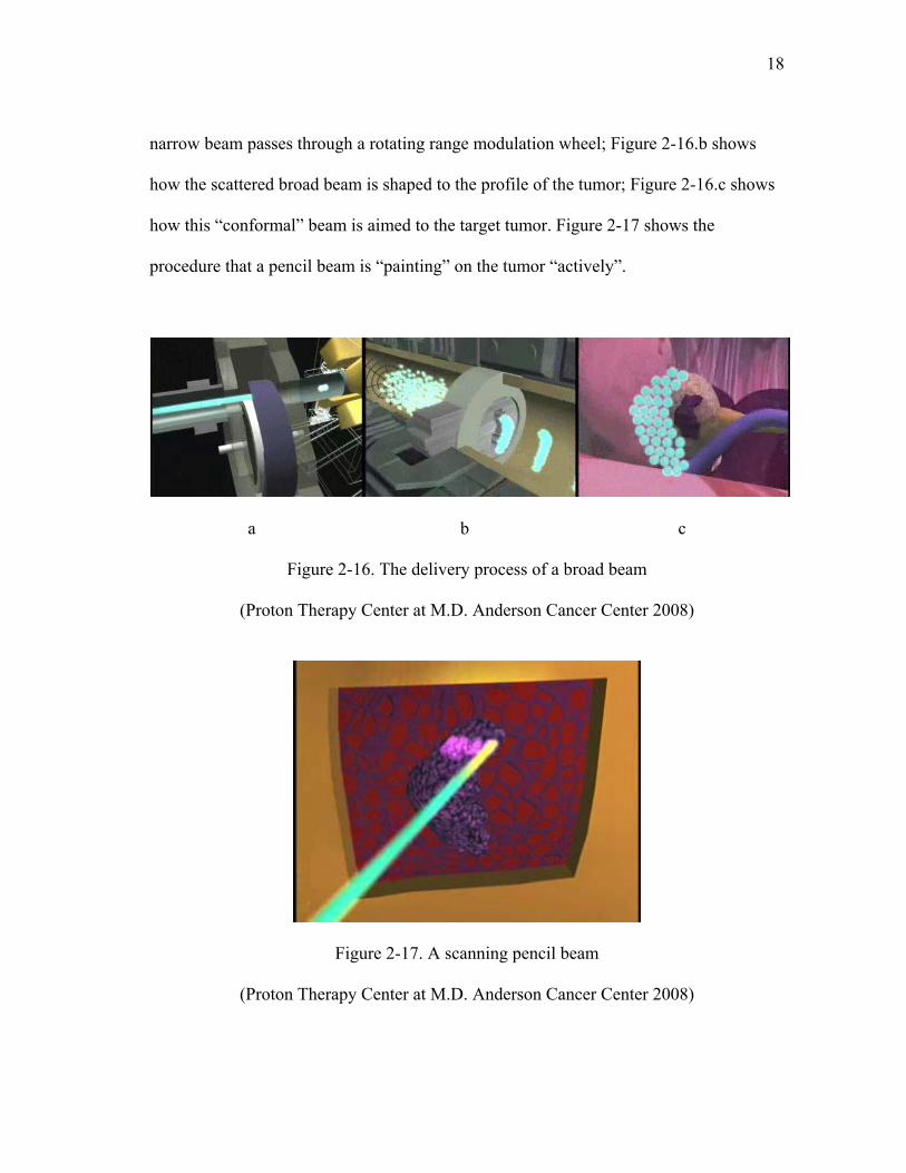
4.2 Fitting Process of SOBP Data by BPW

The measured Bragg-peak data include a large number of data points. Before

these can be read in by the NEU code, the data have to be fitted using the BPW code to

decrease the number of data points. The function of the BPW code is to read in the

measured data and convert them into a cubic spline form.

First, a data file, e.g. “MDA250.txt” containing the 400 pairs of depth-dose data

from 100 MeV case by MCNPX, was set up.

Second, the “bpw.inp”, shown in Figure 4-3, was edited. Only two parameters

were modified: the data file (“MDA250.txt”) and the distance from the source to the

Bragg peak, shown in Table 4-2. On the new fitted SOBP curve, there are only 20 data

pairs by default.

Figure 4-3. Snapshot of “bpw.inp”

36

Table 4-2. Parameters modified in “bpw.inp”

Energy (MeV) Data file name Distance from source to peak (cm) 100 MDA100.txt 307.4 180 MDA180.txt 321.1 250 MDA250.txt 337.3

The routine “bpw.exe” was used to execute the fitting process. Figure 4-4 shows

the execution of BPW code. Figure 4-5 shows the fitting results (marked by open

squares) and related deviations (at bottom) for 250 MeV protons.

Figure 4-4. Execution of the BPW code

37

Figure 4-5. The fitted Bragg curve for 250 MeV protons

The fourth step involved copying the output data files “MDA100.BPK,”

“MDA180.BPK,” and “MDA250.BPK” to the directory of “data.” The snapshot from

“MDA250.BPK” is shown in Figure 4-6.

Figure 4-6. Snapshot of “MDA250.BPK”

38

4.3 Design of Double-Scattering System Using NEU

The theory of multiple scattering is the design basis for a scattering system.

When the beam particles pass through a medium, they can interact with the nuclei of the

medium. Finally, the beam can be deflected in a small angle away from its original

central trajectory. Elastic Coulomb scattering is the main reason for this small-angle

deflection. The deflections lead to the creation of lateral-particle fluence distribution.

The angular distribution of the deflected particles is roughly Gaussian for small

deflection angles (Chu et al. 1993).

The current scattering system includes two components, so it is called “double-

scattering” system. The first scatterer is usually a flat metal foil. According to “multiple

scattering” theory, the particle fluence after the first scatterer is not distributed uniformly

laterally but is best represented by a Gaussian distribution. Thus the dose distribution

laterally will also be Gaussian-shaped. Particles in the central beam need more scattering

to obtain a uniform fluence laterally. A Gaussian-shaped scatterer is added to the beam

line to achieve this goal.

The range modulation wheel is also integrated into the double-scattering system.

It is usually mated on the first scatterer. The benefits of this approach are two-fold:

saving space and decreasing scattering near the patient. This design obeys the principle

of “nozzle with everything upstream.” This combined component is called “S1” in the

NEU code. The Gaussian-shaped (also called contour-shaped) scatterer is called “S2.”

39

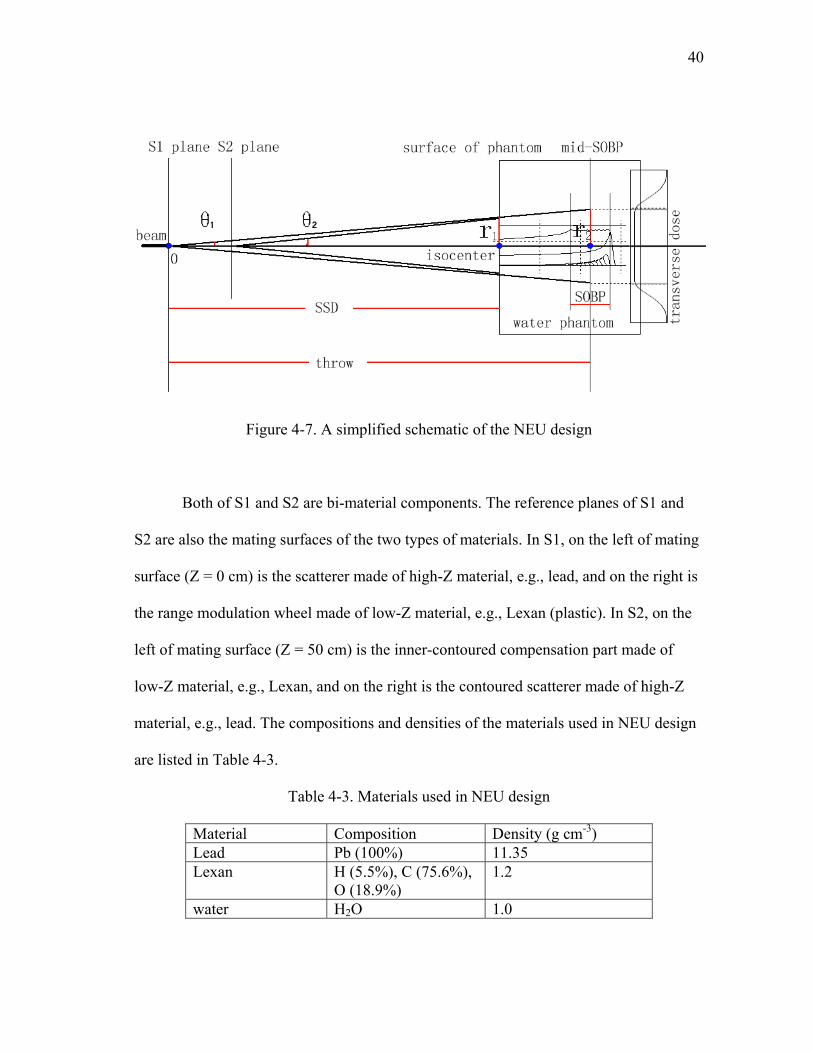
A simplified schematic of the NEU design is shown in Figure 4-7. Notice that, in

NEU design, except the double-scattering system, no other components in a real nozzle

are provided.

The design is actually an interactive process. The user first specifies some

approximate conditional parameters and fixed design goals. Then the user executes the

NEU code to obtain the design results. If the design results are not satisfactory, the user

can modify the input file and execute the code again until the design goals are achieved.

It is a good way to approach the desired results by repeated execution of the code.

The fixed conditional parameters include beam energy, field radius r1 (on the

surface of water phantom), SSD, SOBP width. The approximate conditional parameters

include throw (distance between reference plane of S1 and the middle of SOBP), field

radius r2 (on the plane at mid-SOBP, also called “useful radius”), and the scattering

strengths of S1 and S2. In addition, the NEU code generally assumes the incident beam

is an ideal beam (no size, no angular divergence and perfect steering). Notice that r1 or r2

is the radius at which the transverse dose falls 2.5% below the 100% level on the

corresponding plane, but not the radius of the beam spot on the plane.

40

Figure 4-7. A simplified schematic of the NEU design

Both of S1 and S2 are bi-material components. The reference planes of S1 and

S2 are also the mating surfaces of the two types of materials. In S1, on the left of mating

surface (Z = 0 cm) is the scatterer made of high-Z material, e.g., lead, and on the right is

the range modulation wheel made of low-Z material, e.g., Lexan (plastic). In S2, on the

left of mating surface (Z = 50 cm) is the inner-contoured compensation part made of

low-Z material, e.g., Lexan, and on the right is the contoured scatterer made of high-Z

material, e.g., lead. The compositions and densities of the materials used in NEU design

are listed in Table 4-3.

Table 4-3. Materials used in NEU design

Material Composition Density (g cm-3) Lead Pb (100%) 11.35 Lexan H (5.5%), C (75.6%),

O (18.9%) 1.2

water H2O 1.0

41

In a specified medium, the expected SOBP width cannot be larger than the

maximum range of the beam. Hence, we set three different SOBP widths for the three

beam energies listed in Table 4-4.

Table 4-4. Expected SOBP width

Energy (MeV) SOBP width (cm) 250 10 180 8 100 2

As to the field radius r1, we referred to the design parameters (Zheng et al. 2008)

from M.D. Anderson Cancer Center, listed in Table 4-5. However, in NEU, the useful

radius r2 is used as a parameter, rather than r1. The value of r2 can be approximated. In

Figure 4-7, the tangent of the scattering angle θ1 is:

1 21tan( ) r r

SSD throwθ = = , (1)

so,

12

rr throwSSD

= ⋅ . (2)

Table 4-5. Uncollimated field sizes

Field radius r1 (cm) Large Up to 17.7 Medium Up to 12.75 Small Up to 7.05

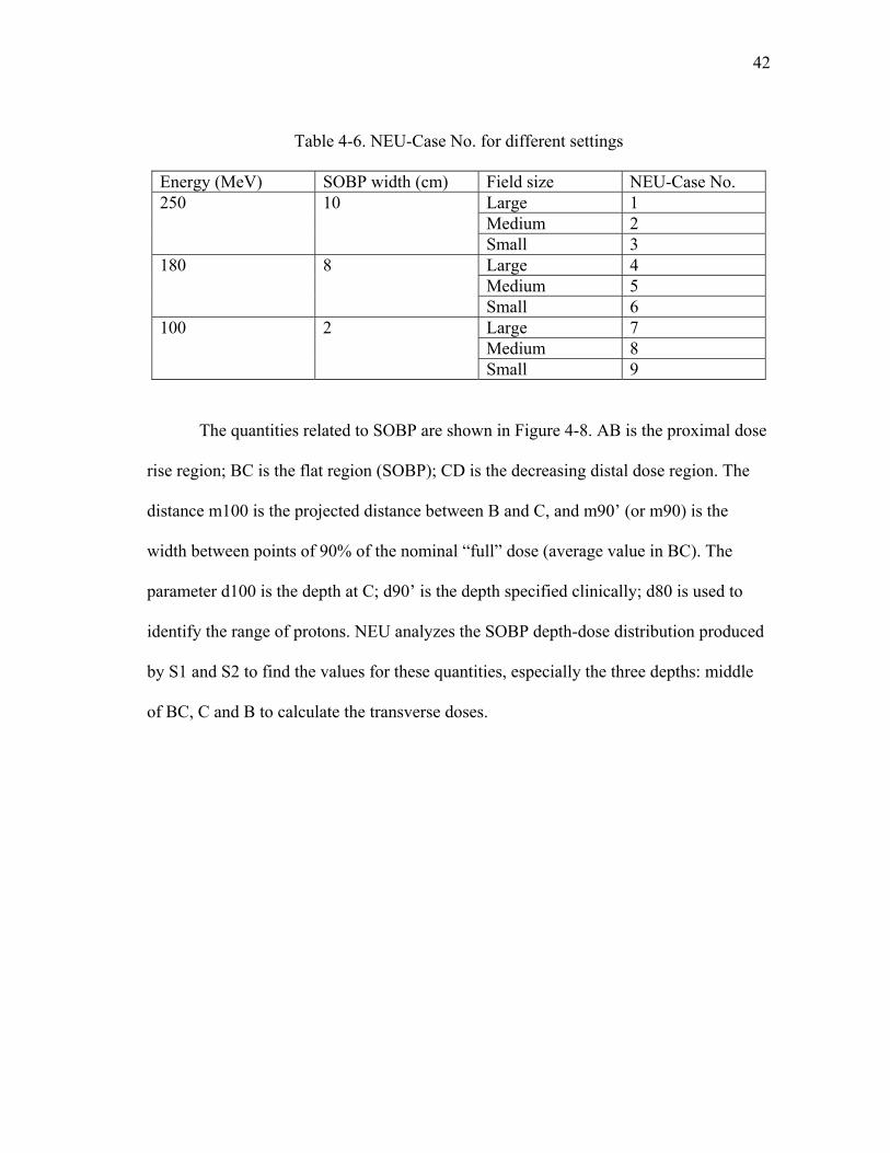
Considering the combinations of energy, SOBP-width, and field size, we

designed nine double-scattering systems listed in Table 4-6.

42

Table 4-6. NEU-Case No. for different settings

Energy (MeV) SOBP width (cm) Field size NEU-Case No. Large 1 Medium 2

250 10

Small 3 Large 4 Medium 5

180 8

Small 6 Large 7 Medium 8

100 2

Small 9

The quantities related to SOBP are shown in Figure 4-8. AB is the proximal dose

rise region; BC is the flat region (SOBP); CD is the decreasing distal dose region. The

distance m100 is the projected distance between B and C, and m90’ (or m90) is the

width between points of 90% of the nominal “full” dose (average value in BC). The

parameter d100 is the depth at C; d90’ is the depth specified clinically; d80 is used to

identify the range of protons. NEU analyzes the SOBP depth-dose distribution produced

by S1 and S2 to find the values for these quantities, especially the three depths: middle

of BC, C and B to calculate the transverse doses.

43

Figure 4-8. Various quantities on a SOBP curve

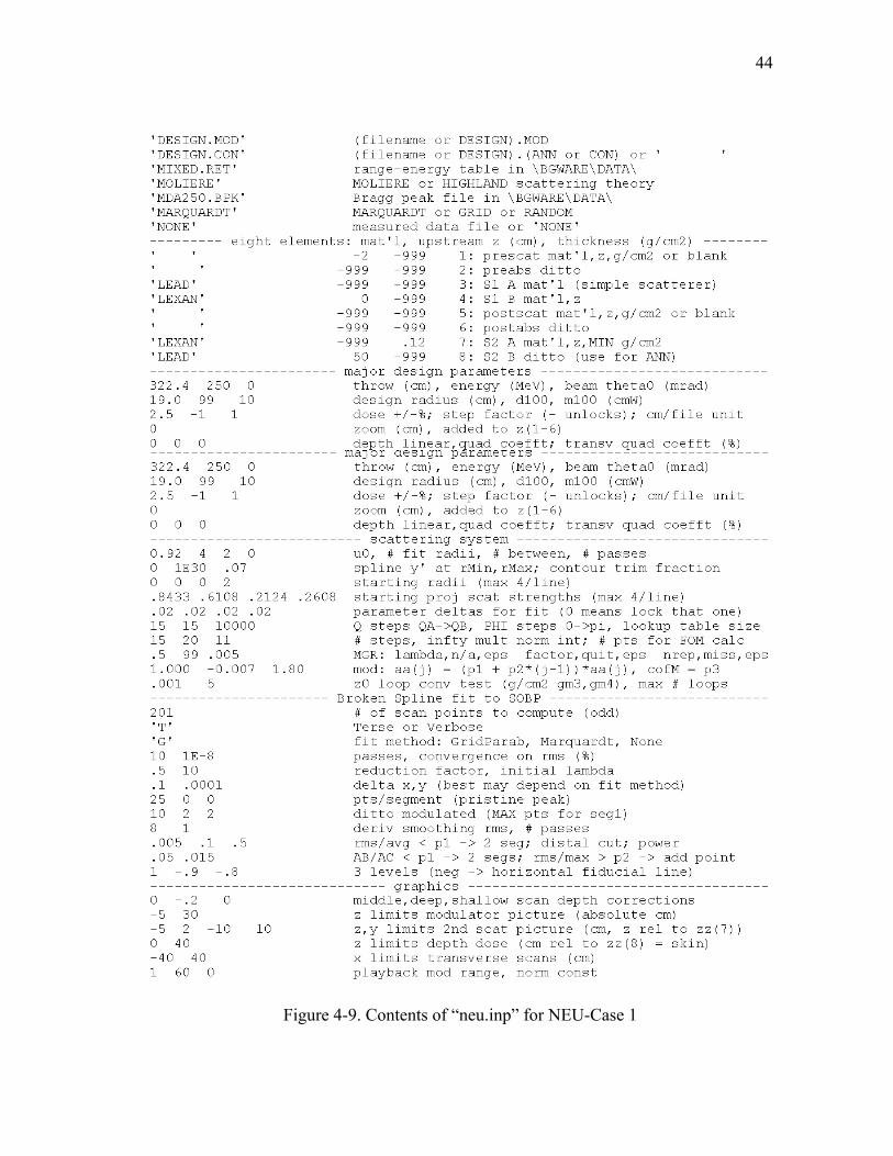
The default input file is “neu.inp.” Besides the parameters mentioned above, the

pristine Bragg-peak data, such as “MDA250.BPK”, dose tolerance interval set at ±2.5%,

some fitting methods, and the number of scan points on the SOBP curve are also

specified in it.

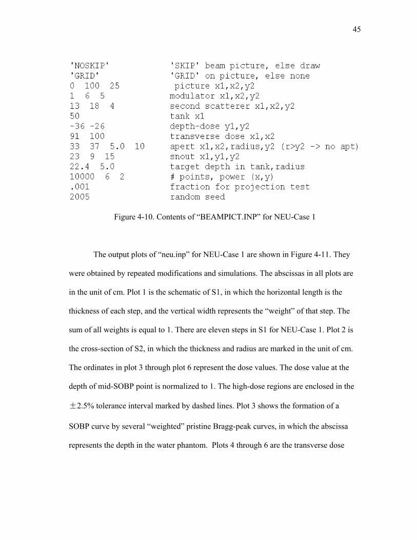
“BEAMPICT.INP” is an optional input file for the NEU code to show a picture

of a schematic beam line for the current simulation. It provides some components

possibly used in a real nozzle, and puts a hypothetical spherical tumor in the water

phantom.

The input files for NEU-Case 1 are shown in Figure 4-9 and 4-10.

44

Figure 4-9. Contents of “neu.inp” for NEU-Case 1

45

Figure 4-10. Contents of “BEAMPICT.INP” for NEU-Case 1

The output plots of “neu.inp” for NEU-Case 1 are shown in Figure 4-11. They

were obtained by repeated modifications and simulations. The abscissas in all plots are

in the unit of cm. Plot 1 is the schematic of S1, in which the horizontal length is the

thickness of each step, and the vertical width represents the “weight” of that step. The

sum of all weights is equal to 1. There are eleven steps in S1 for NEU-Case 1. Plot 2 is

the cross-section of S2, in which the thickness and radius are marked in the unit of cm.

The ordinates in plot 3 through plot 6 represent the dose values. The dose value at the

depth of mid-SOBP point is normalized to 1. The high-dose regions are enclosed in the

±2.5% tolerance interval marked by dashed lines. Plot 3 shows the formation of a

SOBP curve by several “weighted” pristine Bragg-peak curves, in which the abscissa

represents the depth in the water phantom. Plots 4 through 6 are the transverse dose

46

distributions at the scanning depths of proximal, middle and distal points on the SOBP

curve. The abscissas in these three plots represent the radial dimensions.

The beam line is shown in Figure 4-12. It was also obtained by repeated

modifications and simulations. This figure is included only for demonstration, and it

does not reveal the real geometrical size of each component. In addition, the density of

dots standing for the values of dose is exaggerated to make it easy to be understood by

the users.

Figure 4-11. Output plots of “neu.inp” for NEU-Case 1

47

Figure 4-12. Output plot of “BEAMLINE.INP” for NEU-Case 1

One enlarged cross-section of the lead part in S2 for NEU-Case 1 is shown in

Figure 4-13. The abscissa represents the design radius, and the ordinate represents the

corresponding thickness of lead. There are ten design radii numbered from 1 to 10 by

default, but only the first seven thicknesses have non-zero values. Hence, we can use

seven laminated cone frustums marked by 1 to 7 to compose the lead part.

48

Figure 4-13. Cross-section of lead part in S2 for NEU-Case 1

The final satisfactory output parameters for nine NEU cases are listed in Table 4-

7. The results for NEU-Case 5 and 9 are shown in Appendix A.

Table 4-7. The final parameters for 9 NEU cases

NEU-Case No.

Throw (cm)

Useful radius r2 (cm)

Scattering strength of S1(u0)

# of steps in S1

# of lead cells in S2

1 322.4 19.0 0.92 11 7 2 326.7 13.9 0.92 11 7 3 330.5 7.9 0.92 11 6 4 311.65 18.3 0.92 15 7 5 314.0 13.4 0.92 15 7 6 316.2 7.5 0.92 15 6 7 304.5 18 0.92 9 7 8 305.4 13 0.90 9 6 9 306.1 7.2 0.88 9 6

Before proceeding it is necessary to discuss some design tips and limitations of

the NEU code. The most common problem with a double-scattering system is that S1 is

49

poorly matched to S2. The scattering strength of S1 (u0) plays a key role in the forming

of the shape of the transverse dose distribution. Figure 4-14 shows a comparison of

transverse dose distributions from different settings of the scattering strengths of S1 in

NEU-Case 8. If the transverse dose curve looks ‘domed,’ it is because the scattering

strength of S1 is too weak to scatter enough particles laterally. The solving method is to

make S1 a little thicker to increase the scattering strength of S1, at a cost of penetration,

or to move it farther from S2. On the other hand, if the transverse dose curve looks

‘dished,’ it is because the scattering strength of S1 is so strong that too many particles

are scattered from the central line. The remedies are just opposite. One limitation of the

NEU code is that it can be used to deal with only S1 and S2, without any additional

objects or situations that are not cylindrically symmetric.

Figure 4-14. Comparison of transverse doses from different scattering strengths of S1

50

5. MONTE CARLO SIMULATION OF SIMPLIFIED NOZZLE

In this section, we will describe the whole simulation procedure, including

modeling, transport of particles, results visualization, etc., for several nozzles with

different settings. The purpose of Monte Carlo simulation is to verify the design results

from Section 4.

5.1 MCNPX Input File for a Passive-Scattering Nozzle

The contents in an MCNPX input file for a passive nozzle is listed in Table 5-1.

We used “mcnp_pstudy” script to invoke MCNPX, so there was a block for

“mcnp_pstudy” input parameters.

Table 5-1. Contents in an MCNPX input file for a passive nozzle

Block No. contents 1 “mcnp_pstudy” parameters 2 Cell cards to describe all the cells in the problem 3 Surface cards to describe all the surfaces 4 Data cards 4.1 Mode 4.2 Materials 4.3 Coordinate transformation 4.4 Void card to make some unused cells “void” 4.5 Source definition 4.6 Physics setting to specify the Energy ranges and Physics model 4.7 Tally cards to record energy deposition in water phantom, energy and

angular distribution of protons incident on the front surface of water phantom

4.8 Mesh tally cards Particles flux and energy deposition in a designated mesh Multiplication factors for results

4.9 Running control cards

51

5.1.1 Geometry Models

The geometry model used in this research included two parts: a proton beam

delivery system - a nozzle, and a dose measurement system - a water phantom.

The components of a nozzle have been described in Section 2, but the coordinate

system in the MCNPX model was changed. The nozzle was aligned along the X-axis,

and the size of water phantom was 40 cm ×80 cm×80 cm, located at the isocenter. The

components and the materials are listed in Table 5-2. To simulate a proton nozzle as

close as possible to a clinical one, besides the scattering system, some shaping devices

must be added. An outer shell of the nozzle was also needed, which was used to enclose

the beam in a limited space. The thicknesses of dose monitors are usually very small,

and their influence is minor, so they were omitted in the MCNPX model.

The materials listed in Table 5-2 are not the only available ones for a nozzle. For

example, some vendors also use tungsten alloy or brass in first scatterers, and aluminum

alloy is also an alternative for Lexan or ABS resin in the modulation wheels. Table 5-3

lists the composition of materials used in the MCNPX simulations and the CSDA ranges

of 250 MeV protons (Berger et al. 2005).

52

Table 5-2. Components used in a typical passive-scattering-nozzle problem

Name Designed by NEU

Illustrated by NEU

Modeled in MCNPX

Material

Vacuum window Yes Profile monitor Reference monitor First scatterer Yes Yes Yes Lead Range modulation wheel

Yes Yes Yes Lexan

Second scatterer Yes Yes Yes Lead and Lexan

Range shifters Yes ABS resin Collimators Yes Brass Sub dose monitor Main dose monitor Final aperture Yes Yes Brass Range compensator Yes Yes ABS resin Shielding shell Yes Steel water phantom Yes Yes Water

Table 5-3. Composition of materials and CSDA ranges of 250 MeV protons

Material Composition (weight fraction by percent or atomic fraction by number)

Density (g cm-3)

CSDA Range of 250 MeV Protons (g cm-2)

CSDA Range of 250 MeV Protons (cm)

Lead Pb (100%) 11.35 76.69 6.76 Lexan H (5.5%): C (75.6%): O (18.9%) 1.2 38.98(Lucite) 32.5 ABS resin (C3H3N)2:(C4H6)3:(C8H8)5 1.04 37.94(H2O) 36.5 Brass Cu (67%): Zn (33%) 8.35 56.62(Cu) 6.78 Steel Fe(100%), other ingredients are

omitted 7.86 54.54 6.94

air N (75.6%): O (23.1%): Ar (1.3%) 0.001225 42.90 3.50E+04water H2O 1.0 37.94 37.94

In order to observe the influence of different components, three conditions were

set for a nozzle, listed in Table 5-4. First, only S1 and S2 were included in a nozzle to

53

see the dose distribution from an uncollimated scattered beam. Second, a steel outer shell,

several square collimators, and a final cylindrical aperture were added to see the dose

distribution from a collimated broad beam. Third, a “hemi-spherical tumor” was

assumed to be located at a depth in the water phantom, so a range shifter and a patient-

specific range compensator were added to make the high-dose region “conformal” to the

tumor. Notice that the shape of tumor in the MCNPX model was different from the

spherical tumor demonstrated in the NEU model. The parameters of the beam-modifying

devices and the radii of dose-recording regions for different field sizes are listed in Table

5-5.

Table 5-4. Components-in-nozzle conditions in a nozzle for MCNPX

Condition No. Components used in a nozzle 1 S1, S2 2 All except range shifter and patient-specific range compensator 3 all

Table 5-5. Parameters for different field sizes

Field Uncollimated radius of field (cm)

Area of square collimators (cm2)

Inner radius of the final aperture or the patient-specific range compensator (cm)

Radius of dose-recording region in the water phantom (cm)

Large Up to 17.7 25×25 10 15 Medium Up to 12.75 18×18 7 10 Small Up to 7.05 10×10 4 6

54

In order to understand the different characteristics of the treatment beam, several

types of tallies were used in MCNPX to obtain the desired quantities in selected regions

in the water phantom. The tally-geometry conditions are listed in Table 5-6.

Figure 5-1 is a schematic of the rectangular mesh tally in the water phantom.

Figure 5-2 is a schematic of the meshes used to score depth dose along the central axis

(X-axis), and transverse doses at different depths. The whole model is cylindrically

symmetric along the X-axis, so any symmetric layer along the X-axis can be used to

score the transverse dose. Here, we used X-Z (fixed-Y) layer. Red meshes are used to

score and show depth-dose distribution (SOBP-curve) along the central axis (X-axis),

and blue meshes are used to score and show the transverse-dose distribution crossing the

proximal, middle, and distal points on the SOBP-curve. The transverse layer in Figure 5-

3 was used to show the contoured distribution of fluence or dose. Figure 5-4 is a general

schematic of the scoring planes (or layers) in a mesh tally. The numbers of meshes

shown in these figures are only used to illustrate the rectangular meshes, and they are not

the real number of meshes used in the mesh tally.

55

Table 5-6. Tally-geometry conditions

Condition No. tally region Tally type Quantity to score Unita F1 (E1, Fm1) Current (Energy

spectrum of incident protons)

# in the specified energy bin

The front surface

F11 (*C11, Fm11) Current (Angular distribution spectrum of incident protons)

# in the specified angle bin

1

Whole water phantom

F6 (Fm6) Absorbed dose MeV g-1

Mesh tally (type 1) Fluxb

Fluence in a mesh # cm-2 2 (Figure 5-2)

X: 300~340 Y: -0.5~0.5 Z: -39.5~39.5 The number of meshes is 80×1×79.

Mesh tally (type 1) PEDEPc

Energy deposition in a mesh

MeV cm-3

Mesh tally (type 1) Flux

Fluence in a mesh # cm-2 3d (Figure 5-3)

X: 321~321.5 Y: -39.5~39.5 Z: -39.5~39.5 The number of meshes is 1×79×79.

Mesh tally (type 1) PEDEP

Energy deposition in a mesh

MeV cm-3

Mesh tally (type 1) Flux

Fluence in a mesh # cm-2 4 (Figure 5-4)

The number of meshes is listed in Table 5-7.

Mesh tally (type 1) PEDEP

Energy deposition in a mesh

MeV cm-3

a The tally results are normalized to the results by one source particle. b In MCNPX, the result from “Flux” is “fluence” if omitting time. c The result from “PEDEP” (MeV cm-3) equals to absorbed dose (MeV g-1) if the medium is water. d Condition 3 is used to see the function of a single step of S1 (scattering part) alone and combined S1 (a single step of scattering part) and S2.

56

Table 5-7. Parameters for mesh tally by collimated beams

Field size Energy (MeV) Axis Coordinate range (cm)

Number of binsa

250 X 300 ~ 330 60 180 X 300 ~ 320 40 100 X 300 ~ 308 16 Allb Y -15 ~ 15 30

large

All Z -15 ~ 15 30 250 X 300 ~ 335 70 180 X 300 ~ 325 50 100 X 300 ~ 309 18 All Y -10 ~ 10 20

medium

All Z -10 ~ 10 20 250 X 300 ~ 340 80 180 X 300 ~ 325 50 100 X 300 ~ 309 18 All Y -6 ~ 6 12

small

All Z -6 ~ 6 12 a All the meshes have the same size: 0.5 cm×1 cm×1 cm. b “All” represents all the energies of 100, 180 and 250 MeV.

Figure 5-1. Illustration of the geometry for a rectangular mesh tally

57

Figure 5-2. Fixed-Y layer for depth-dose and transverse dose

Figure 5-3. Fixed-X layer for transverse dose

58

Figure 5-4. Planes to show dose or fluence distribution

Fifteen MCNPX cases were used to simulate the problems with different nozzle

settings. A parallel-broad-beam case without a nozzle was also simulated, numbered by

MCNPX-Case 0, in which the size of each mesh was 2 mm×2 mm×2 mm. All the

sixteen MCNPX cases are listed in Table 5-8.

59

Table 5-8. Cases simulated by MCNPX

Energy (MeV)

Components-in-nozzle condition No.

Field size Tally-geometry condition No.

MCNPX-Case No.

100 None Beam radius is 2 cm

Mesh: 2 mm×2 mm×2 mm

0

Large 1, 2, 3 1 Medium 1, 2 2

1

Small 1, 2 3 Large 4 4 Medium 4 5

2

Small 4 6 Large 4 7 Medium 4 8

250

3

Small 4 9 Large 4 10 Medium 4 11

180 2

Small 4 12 Large 4 13 Medium 4 14

100 2

Small 4 15

The distance between the source and the front surface of the water phantom, the

center of which was defined as isocenter, was 300 cm. The parameters of S1 and S2

were obtained from the NEU-design results. The results for NEU-Case 1 (250 MeV,

large field), used in MCNPX-Case 1, 4 and 7, are listed in Table 5-9. The modeling of

S2 was the most difficult part in the whole modeling process. A series of superimposed

“truncated right-angle” cones were used to compose the S2. The parameters of other

components can be found in Appendix B.

60

Table 5-9. Parameters of S1 and S2 from NEU-Case 1

S1 S2 Thickness (cm) Thickness (cm) Step No. weight Lead Lexan

Radius (cm) Lexan Lead

1 0.4006 0.8829 0 0 0.1002 0.8731 2 0.1378 0.8679 0.9377 0.5331 0.4135 0.811 3 0.0965 0.8515 1.8827 1.0662 1.2238 0.6505 4 0.0739 0.8344 2.8317 1.5993 2.2867 0.4397 5 0.0608 0.8166 3.7842 2.1324 3.3258 0.2334 6 0.0513 0.7982 4.7402 2.6655 4.071 0.0853 7 0.0437 0.7791 5.6996 3.1986 4.4633 0.0073 8 0.0379 0.7593 6.6627 3.7317 4.5001 0 9 0.0343 0.7388 7.6294 4.2648 4.5001 0 10 0.0287 0.7176 8.6003 4.7979 4.5001 0 11 0.0344 0.6956 9.5754 To avoid the input error, if the thickness is 0, it is set to 0.0001 in MCNPX.

To avoid the sharpness in the first cell, the radius of 0 is set to 0.001 in MCNPX input.

5.1.2 Proton Beam Source Definition

As stated in Section 2, the production of secondary neutrons and recoil nuclei

was not considered in this research. “Mode H” was used to indicate that protons were the

only tracked particles. In MCNPX, there is no explicit generation of “delta-ray” knock-

on electrons as trackable particles for heavy charged particles, and delta rays are

produced only for electrons.

The particle-source description was based on the source at M.D. Anderson

Cancer Center. One surface vertical to X-axis was set as the source plane. The spatial

distribution of the proton source was described by two Gaussian distributions with a

FWHM value of 0.54 cm in the Y-direction and 1.22 cm in the Z-direction. A “cookie-

cutter” cell was defined to limit the position of the starting source particles to a radius of

3 cm around the beam axis. The energy of the source was also described by a Gaussian

61

distribution. The FWHM ranges from 0.23% to 0.3% for nominal energies from 250

MeV to 100 MeV (Titt et al. 2008). The FWHM for 180 MeV proton beam was assumed

to be 0.27%. In MCNPX, the formats for the spatial and energy Gaussian distribution

functions are different. For the spatial distribution, the input parameters are the mean

value and the FWHM (2.35σ), but for energy, the input parameters are the mean value

and 1.414σ. The parameters for the energy Gaussian distributions are listed in Table 5-

10. The descriptions of the spatial and energy distributions in MCNPX are shown in

Figure 5-5. The spatial distribution of the proton source (one thousand particles) is

shown in Figure 5-6, in which the radius of the circle is 3 cm. The probability density

function of energy (250 MeV) distribution is shown in Figure 5-7.

Table 5-10. Parameters for energy Gaussian distributions

Energy (MeV) FWHM=2.35 σ (MeV) 1.414 σ (MeV) 100 0.3 0.184 180 0.486 0.292 250 0.575 0.346

Figure 5-5. The spatial and energy distribution functions in MCNPX

62

Figure 5-6. The spatial Gaussian distribution of proton source on Y-Z plane

250 MeV, FWHM = 0.575 MeV

0

0.2

0.4

0.6

0.8

1

1.2

1.4

1.6

1.8

248.5 249 249.5 250 250.5 251 251.5

Figure 5-7. The energy Gaussian distribution (250 MeV)

However, if the spatial and energy distributions of the source are complex, i.e.,

both are Gaussian distributions, the sampling process of particles can require a large

amount of time. To save time but not to affect the simulation results seriously, an ideal

63

beam source (the same beam as in NEU code) was used instead of the Gaussian-

distributed source in all the cases with a nozzle.

5.1.3 Physics Settings

The “phys:h” card can be used to control some physics settings in proton-

transport problems. The default upper energy limit is 100 MeV for protons. It must be

increased to a higher value to simulate problems with 250 MeV protons. The parameter

“emax” was changed to “300 MeV” to cover all the problems to be simulated. For the

“table-based physics cutoff”, the “mix and match” option was still kept by default to

assure either tables or models can be used when available. For protons, “la150h” is the

data library containing the data tables for several isotopes. In addition, the “Vavilov”

model, which is the default, was kept to control charged-particle straggling, rather than

“CSDA”, and the production of recoil light ions was inhibited by default.

The “cut:h” card can be used to set the energy cutoff. The default lower energy

cutoff for protons is 1 MeV. This cutoff was retained in MCNPX-Case 0. In other cases,

to save the computation time, the cutoff was increased to 20 MeV, within a range of 4.3

mm in water, which was shorter than the maximum size of a mesh (5 mm) in mesh tally.

In MCNPX, five cards (LCA, LCB, LCC, LEA and LEB) can be used to control

physics parameters for the “Bertini”, “ISABEL”, “CEM03”, “INCL4”and “FLUKA”

options (the version of FLUKA in MCNPX is kept for legacy purposes.). In this research,

only “CEM03” or “INCL4” models can be chosen to run the problem correctly. The

problems with “Bertini” or “ISABEL” models aborted in the running in this research.

64

The reason for failure is still unclear. Simulation results from the “CEM03” and

“INCL4” models had a minor discrepancy, while the problems with “CEM03” took less

time, so the “CEM03” model was adopted finally. Only the LCA, LCB and LEA cards

were used in this research.

5.1.4 Tally Types

As given in Table 5-1 and Table 5-6, in this research the F1 tally was used to

record the current of particles across a surface. The F1 tally and energy bin (E1) were

used to obtain the energy spectrum, and the F1 and angle bin (*C1) were used to obtain

the angular distribution of the protons incident on the front surface of water phantom.

The F6 tally (energy deposition in unit mass) was added also to record the average

absorbed dose in the water phantom.

To obtain the “cell-wise” fluence and dose distributions, we used Mesh tally

(type 1) in MCNPX. Mesh tally is a method to score the quantities of interest, such as

fluence, energy deposition, and number of tracks in the volume of the mesh. One mesh

can contain several different materials, so the mesh tally result is not averaged over the

mass of the mesh, but over the volume of the mesh. There are three types of mesh

geometries: rectangular mesh, cylindrical mesh and spherical mesh. A rectangular-mesh

geometry built on the water phantom was used in this research.

Actually, to obtain unbiased tally results, we set the number of steps in S1 as the

multiplication factor for all the tallies by using Fm cards. The reason will be explained in

Section 5.4.

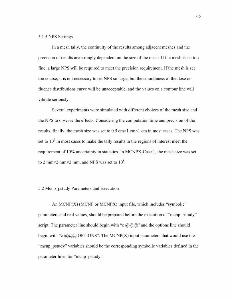
65

5.1.5 NPS Settings

In a mesh tally, the continuity of the results among adjacent meshes and the

precision of results are strongly dependent on the size of the mesh. If the mesh is set too

fine, a large NPS will be required to meet the precision requirement. If the mesh is set

too coarse, it is not necessary to set NPS so large, but the smoothness of the dose or

fluence distributions curve will be unacceptable, and the values on a contour line will

vibrate seriously.

Several experiments were simulated with different choices of the mesh size and

the NPS to observe the effects. Considering the computation time and precision of the

results, finally, the mesh size was set to 0.5 cm×1 cm×1 cm in most cases. The NPS was

set to 107 in most cases to make the tally results in the regions of interest meet the

requirement of 10% uncertainty in statistics. In MCNPX-Case 1, the mesh size was set

to 2 mm×2 mm×2 mm, and NPS was set to 108.

5.2 Mcnp_pstudy Parameters and Execution

An MCNP(X) (MCNP or MCNPX) input file, which includes “symbolic”

parameters and real values, should be prepared before the execution of “mcnp_pstudy”

script. The parameter line should begin with “c @@@” and the options line should

begin with “c @@@ OPTIONS”. The MCNP(X) input parameters that would use the

“mcnp_pstudy” variables should be the corresponding symbolic variables defined in the

parameter lines for “mcnp_pstudy”.

66

Before the execution of this script, the user should confirm if “Perl” is installed

under the UNIX system. The user can use the command “which perl” to check it, and

usually the default location is “/usr/bin/perl.” If Perl cannot be found, it must be installed

before using “mcnp_pstudy”. The execution command of “mcnp_pstudy” is “perl

mcnp_pstudy -i inputfile.” Several other optional parameters can be added after this

command or specified in an input file.

The execution process of “mcnp_pstudy” includes three stages: setup, invoking

and data collection. If “-setup” is specified, a series of case directories will be created

and the real values are assigned to the symbolic parameters to produce one real

MCNP(X) input file named “inp” in each case directory. If “-run” is specified, an

MCNP(X) command will be invoked to execute all the “inp” files successively. If “-

collect” is specified, the data will be collected and the average tally results and relative

errors will be created and shown. Currently, the specification of “-collect” is invalid to

the mesh tally results in MCNPX but valid to the tallies in MCNP.

5.3 Visualization of Models

The purpose of visualization of these models is to find the errors in the geometry

and to observe the tracks of particles.

In each MCNPX case, one input file in a sub-directory was chosen randomly as

the input file for Visual Editor of MCNPX to see the geometries and tracks. Sub-case 5

in MCNPX-Case 7 was taken as an example. The 3D model is shown in Figure 5-8. Due

to a deficiency of Visual Editor, the final aperture and patient-specific compensator

67

cannot be shown in the 3D model. The 2D cross sectional profiles of different

components are shown in Figure 5-9 through Figure 5-12. The fifth step in S1 included

two parts: a scattering foil and a range modulation part. The bi-material contour-shaped

S2 can be seen clearly. The collimator for S2 was a cylindrical ring surrounding S2, but

the other three collimators are rectangular frames. The final aperture is a rectangular

solid with a cylindrical hole. The patient-specific compensator is set to be a rectangular

solid with a subtraction of a hemisphere. The compositions of the components were

consistent with the data in Table 5-3.

Figure 5-8. 3D model of a passive-scattering nozzle in MCNPX-Case 7

Figure 5-9. Schematic of one step on S1

68

Figure 5-10. Schematic of a contour-shaped S2

Figure 5-11. Schematic of collimator and range shifter

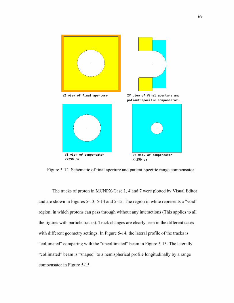
69

Figure 5-12. Schematic of final aperture and patient-specific range compensator

The tracks of proton in MCNPX-Case 1, 4 and 7 were plotted by Visual Editor

and are shown in Figures 5-13, 5-14 and 5-15. The region in white represents a “void”

region, in which protons can pass through without any interactions (This applies to all

the figures with particle tracks). Track changes are clearly seen in the different cases

with different geometry settings. In Figure 5-14, the lateral profile of the tracks is

“collimated” comparing with the “uncollimated” beam in Figure 5-13. The laterally

“collimated” beam is “shaped” to a hemispherical profile longitudinally by a range

compensator in Figure 5-15.

70

Figure 5-13. Nozzle geometry and proton tracks in MCNPX-Case 1

Figure 5-14. Nozzle geometry and proton tracks in MCNPX-Case 4

71

Figure 5-15. Nozzle geometry and proton tracks in MCNPX-Case 7

5.4 Execution of Merge_mctal

As mentioned previously, in a problem including an N-step range modulation

wheel, the problem is separated into N cases, so the expected result from all the cases

should be:

1

N

i ii

D W=

= ∑ D , (3)

where is the weight of the ith step; is the corresponding score, such as

fluence or dose; is the weighted score from the ith step; N is the total steps in a

wheel; the known condition is

iW iD

i iW D

1

1N

ii

W=

=∑ .

72

The function of “merge_mctal” script is to sum the “mctal” data from N cases

and average the sum by N to create a new “mctal” data file. If so, the results from

“merge_mctal” will be:

1

1 N

merge i ii

D W DN N=

= =∑ 1 D , (4)

which is not the expected result. The expected result has been reduced by a factor

of 1N

. If a multiplication factor N is set for each tally, the ith result for the ith case will be

. The result from “merge_mctal” will be: i iW D N

1 1

1 N N

i i i ii i

W D N W D DN = =

=∑ ∑ = , (5)

which is the expected result. Hence, to obtain unbiased results, a multiplication

factor N must be set in Fm cards for all the tallies. For problems whose results did not

need to be merged by “merge_mctal”, this multiplication factor was not set.

After execution of “mcnp_pstudy,” the tally results for each sub-case are stored

in a UNIX-format file “mctal.” All the “mctal” files were renamed with successive

numbers, such as “mctal01”, “mctal02”, etc; copied to a folder named “merge”

containing “merge_mctal” and an executable script “mergecsh” including the command

to execute “merge_mctal.”

Because the alignment format of the contents in a “mctal” file from MCNPX is

different from the one from MCNP, “merge_mctal” cannot be directly used to merge

“mctal” files from MCNPX. The codes on the 368th line of the source code of

“merge_mctal” revealed that “merge_mctal” did not read the parameters after “f” for F5

73

tally. In addition, the format of source particle types was the main difference between

MCNP and MCNPX. Hence, the solving method was to change the particle types to

MCNP format and modify the mesh tally in MCNPX to “F5” tally.

After the execution of “merge_mctal,” a new “mctal” file was produced. To

make this new “mctal” file to be read in by MCNPX, it must be changed back to

MCNPX format. The method was to replace the first paragraph with the contents from

an original “mctal” file from MCNPX.

5.5 Simulation Results

Several methods can be used to view the simulation results. The first is to

execute the command “mcnpx z” in the directory containing the “mctal” file to view the

results graphically. The second method is to read in the data by a “VB script embedded

in Excel” edited by the author of this thesis. Before using VB script, the “mctal” file

must be converted to “DOS” format from “UNIX” format. The third method is to invoke

one subroutine of MCNPX - “gridconv” to convert the “mdata” file (a binary file storing

the mesh tally data) to an ASCII file compatible with several external graphics packages,

such as “PAW”, “IDL”, “Tecplot” or “GNUPLOT.” The packages “IDL” and “Tecplot”

were preferred because the formats for these packages are more readable.

74

5.5.1 Results No. 1

The first set of results came from MCNPX-Case 0. Only a broad beam and a

water phantom were provided. The proton energy was 100 MeV, and the beam radius

was 2 cm. The contour depth-dose distribution on the central layer and the contour

transverse dose distribution at a depth of 5 cm are shown in Figure 5-16 and Figure 5-17.

The depth-dose distribution along the central axis (X-axis) and the transverse dose

distribution at a depth of 7.6 cm along the Y-axis are shown in Figure 5-18 and Figure 5-

19. These results are consistent with the theoretical expectations qualitatively.

Figure 5-16. Contour depth-dose distribution on the central layer

75

Figure 5-17. Contour transverse dose distribution at the depth of 5 cm

76

Figure 5-18. The depth-dose distribution along the central axis (X-axis)

77

Figure 5-19. The transverse dose distribution at the depth of 7.6 cm along the Y-axis

5.5.2 Results No. 2

The second set of results came from MCNPX-Case 1 with tally-geometry

condition No. 3. A narrow beam with an energy of 250 MeV and the first step of S1

(scattering part) were provided. MCNPX and “gridconv” were invoked to deal with the

data. The converted data from “gridconv” were plotted using Excel in 2D or 3D mode.

78

The geometry and tracks are shown in Figure 5-20. The contour transverse dose

distribution (X: 321 ~ 321.5 cm) from MCNPX is shown in Figure 5-21. The results

plotted using Excel are shown in Figure 5-22 in 2D mode and Figure 5-23 in 3D mode.

The transverse dose along the Y-axis (X: 321 ~ 321.5 cm, Z: -0.25 ~ 0.25 cm) from

MCNPX is shown in Figure 5-24.

Figure 5-20. Geometry and tracks of protons scattered by a scattering foil

Figure 5-21. The contour transverse dose distribution for Results No. 2

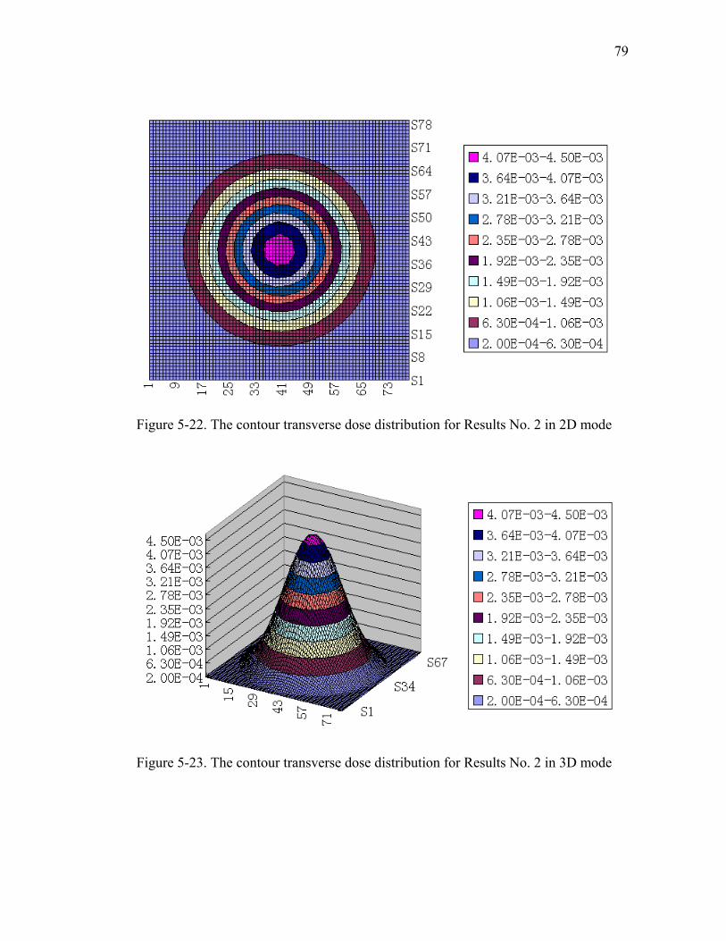
79

Figure 5-22. The contour transverse dose distribution for Results No. 2 in 2D mode

Figure 5-23. The contour transverse dose distribution for Results No. 2 in 3D mode

80

Figure 5-24. The transverse dose along the Y-axis for Results No. 2

From these figures, it was determined that the transverse dose distribution had a

Gaussian shape rather than a uniform-spreading shape if only a single scattering foil was

used. The high-dose region from this scattered beam was so narrow that this beam

possibly can be used to only treat tumors with small sizes.

81

5.5.3 Results No. 3

Based on the settings for the second set of results, an S2 was added to produce

the third simulation results. The geometry and tracks are shown in Figure 5-25. The

contour transverse dose distribution (X: 321 ~ 321.5 cm) is shown in Figure 5-26. The

transverse dose along the Y-axis (X: 321 ~ 321.5 cm, Z: -0.25 ~ 0.25 cm) is shown in

Figure 5-27.

Figure 5-25. Geometry and tracks of protons scattered by a scattering foil and S2

82

Figure 5-26. The contour transverse dose distribution for Results No. 3

83

Figure 5-27. The transverse dose along the Y-axis for Results No. 3

From these figures, it can be seen that the introduction of S2 helped to flatten the

beam to produce a flat transverse dose distribution. The high dose at the middle point

seemed to have been added to the lateral points. This flat beam can be used to treat

tumors with relative large sizes.

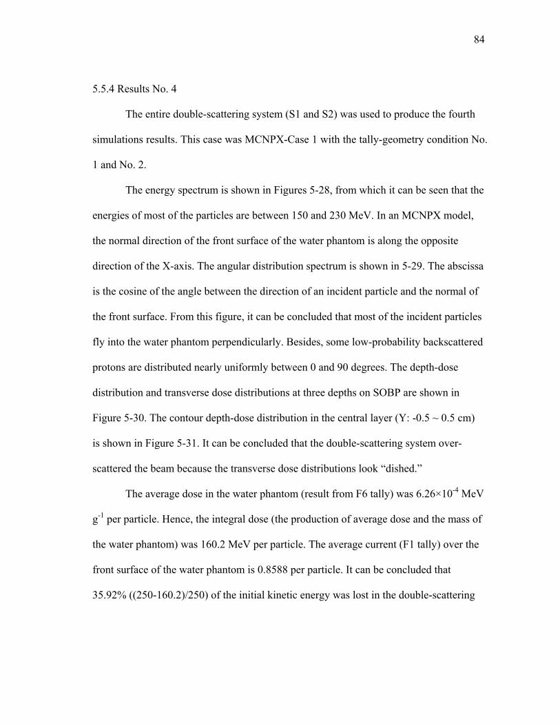
84

5.5.4 Results No. 4

The entire double-scattering system (S1 and S2) was used to produce the fourth

simulations results. This case was MCNPX-Case 1 with the tally-geometry condition No.

1 and No. 2.

The energy spectrum is shown in Figures 5-28, from which it can be seen that the

energies of most of the particles are between 150 and 230 MeV. In an MCNPX model,

the normal direction of the front surface of the water phantom is along the opposite

direction of the X-axis. The angular distribution spectrum is shown in 5-29. The abscissa

is the cosine of the angle between the direction of an incident particle and the normal of

the front surface. From this figure, it can be concluded that most of the incident particles

fly into the water phantom perpendicularly. Besides, some low-probability backscattered

protons are distributed nearly uniformly between 0 and 90 degrees. The depth-dose

distribution and transverse dose distributions at three depths on SOBP are shown in

Figure 5-30. The contour depth-dose distribution in the central layer (Y: -0.5 ~ 0.5 cm)

is shown in Figure 5-31. It can be concluded that the double-scattering system over-

scattered the beam because the transverse dose distributions look “dished.”

The average dose in the water phantom (result from F6 tally) was 6.26×10-4 MeV

g-1 per particle. Hence, the integral dose (the production of average dose and the mass of

the water phantom) was 160.2 MeV per particle. The average current (F1 tally) over the

front surface of the water phantom is 0.8588 per particle. It can be concluded that

35.92% ((250-160.2)/250) of the initial kinetic energy was lost in the double-scattering

85

system in average, and 85.88% of the source particles can deposit energy in the water

phantom.

Figure 5-28. The energy spectrum of incident protons in water phantom

86

Figure 5-29. The angular distribution spectrum of incident protons in water phantom

87

Figure 5-30. The depth-dose and transverse dose distributions for Results No. 4

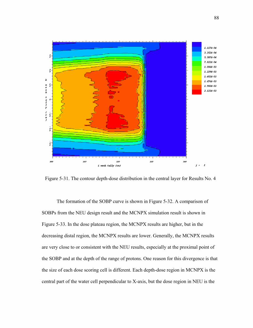
88

Figure 5-31. The contour depth-dose distribution in the central layer for Results No. 4

The formation of the SOBP curve is shown in Figure 5-32. A comparison of

SOBPs from the NEU design result and the MCNPX simulation result is shown in

Figure 5-33. In the dose plateau region, the MCNPX results are higher, but in the

decreasing distal region, the MCNPX results are lower. Generally, the MCNPX results

are very close to or consistent with the NEU results, especially at the proximal point of

the SOBP and at the depth of the range of protons. One reason for this divergence is that

the size of each dose scoring cell is different. Each depth-dose region in MCNPX is the

central part of the water cell perpendicular to X-axis, but the dose region in NEU is the

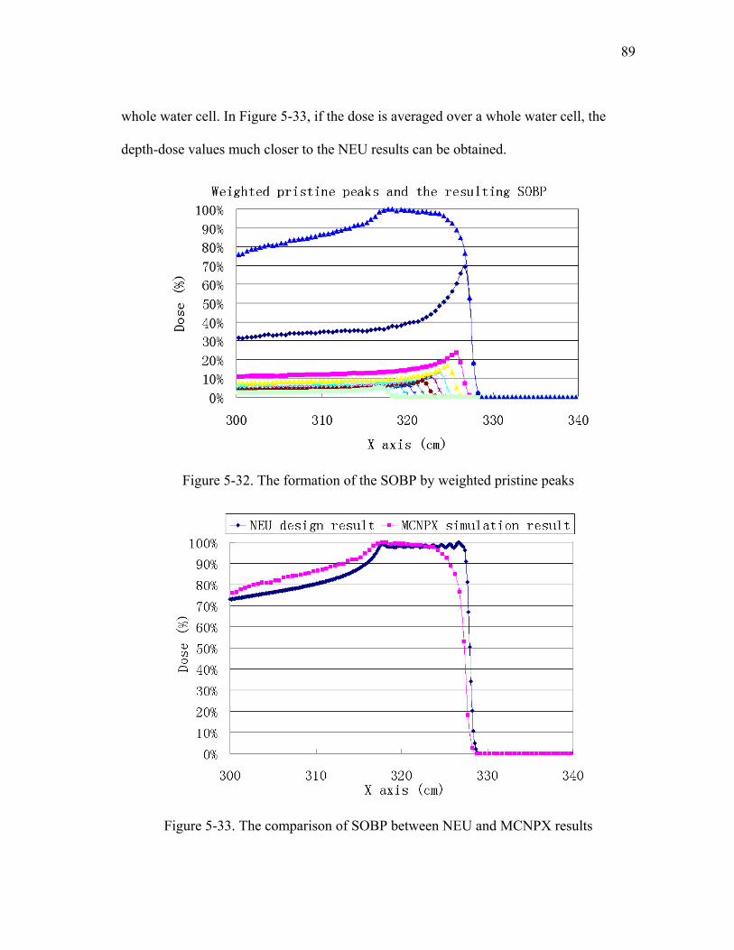
89

whole water cell. In Figure 5-33, if the dose is averaged over a whole water cell, the

depth-dose values much closer to the NEU results can be obtained.

Figure 5-32. The formation of the SOBP by weighted pristine peaks

Figure 5-33. The comparison of SOBP between NEU and MCNPX results

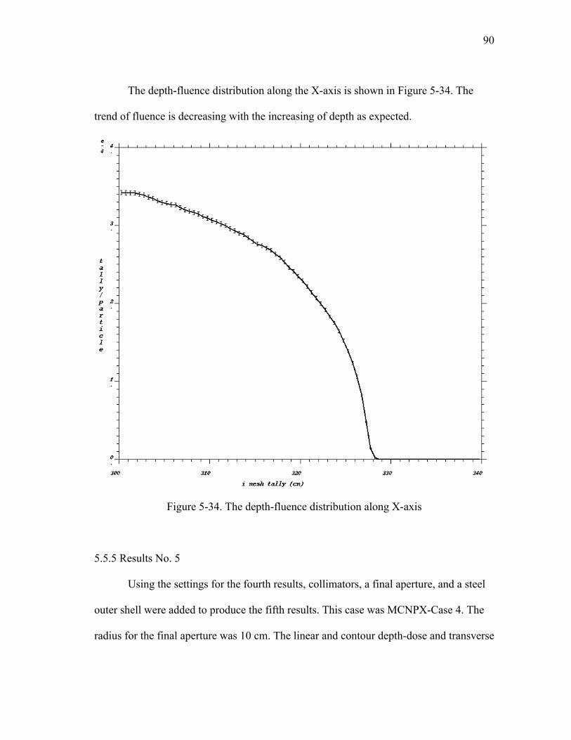
90

The depth-fluence distribution along the X-axis is shown in Figure 5-34. The

trend of fluence is decreasing with the increasing of depth as expected.

Figure 5-34. The depth-fluence distribution along X-axis

5.5.5 Results No. 5

Using the settings for the fourth results, collimators, a final aperture, and a steel

outer shell were added to produce the fifth results. This case was MCNPX-Case 4. The

radius for the final aperture was 10 cm. The linear and contour depth-dose and transverse

91

dose distributions are shown in Figure 5-35 and Figure 5-36. From these figures, it can

be seen that the field radius is about 12 cm, a little larger than the radius of the final

aperture due to the scattering effect; the range of protons is 28 cm; the uniformity of the

transverse dose at the distal SOBP is the worst in the three transverse dose plots.

Figure 5-35. The depth-dose and transverse dose distributions for Results No. 5

92

Figure 5-36. The contour dose distributions for Results No. 5

5.5.6 Results No. 6

Using the settings for the fifth results, a range shifter and a patient-specific

compensator were added to produce the sixth results. This case was MCNPX-Case 7. A

hypothetical hemispherical tumor with a radius of 10 cm was located in the water

phantom centered at 315 cm on the X-axis. A 1 cm long range shifter (made of ABS

resin with a density of 1.04 g cm-3) and an inner-hemispherical patient-specific

compensator with a radius of 10 cm were added in the nozzle. The linear and contour

depth-dose distributions are shown in Figure 5-37 and Figure 5-38. The contour

93

transverse dose distributions are shown in Figure 5-39. From these figures, it was

concluded that the proton range was about 27 cm and profiles of the outer-dose contours

were hemispherical. Hence, the high-dose region was nearly “conformal” to the

hemispherical tumor.

Figure 5-37. The depth-dose distribution for Results No. 6

94

Figure 5-38. The contour depth-dose distribution for Results No. 6

95

Figure 5-39. The contour transverse dose distributions at different depths

5.5.7 Results No. 7

The seventh results came from MCNPX-Case 11. The beam energy was 180

MeV; the radius of the final aperture was 7 cm; the expected SOBP width was 8 cm. The

VB script embedded in Excel was used to analyze this case. The dose distributions in the

central layer are shown in Figure 5-40 and the relative errors are shown in Figure 5-41.

“i” or “j” is the mesh number in the corresponding dimension. Only near the decreasing

96

distal part were the relative errors higher than 10%. The depth-dose distribution plotted

using MCNPX is shown in Figure 5-42.

Figure 5-40. The dose distributions in the central layer plotted by Excel

Figure 5-41. The relative errors for dose distributions in the central layer

97

Figure 5-42. The depth-dose distributions in the central layer plotted by MCNPX

5.5.8 Results No. 8

The eighth results came from MCNPX-Case 15. The beam energy was 100 MeV;

the radius of the final aperture was 4 cm; the expected SOBP width was 2 cm. The

depth-dose distribution is shown in Figure 5-43. The contour transverse dose distribution

at mid-SOBP is shown in Figure 5-44. It can be found that the shape of SOBP was not as

flat as expected with the NEU design, but the transverse dose was still flat.

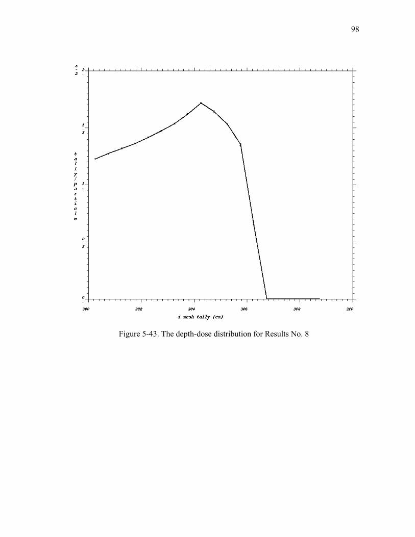
98

Figure 5-43. The depth-dose distribution for Results No. 8

99

Figure 5-44. The contour transverse dose distribution for Results No. 8

100

6. SUMMARY AND FUTURE WORK

6.1 Summary

Even though the scanning technique in proton therapy is more advanced, the

passive-scattering nozzle is still used more widely. It is very significant to concern the

design and simulation of a passive-scattering nozzle.

The double-scattering system is a key component in a passive-scattering nozzle

for proton therapy. The first scatterer is used to broaden the narrow beam, and the

second scatterer is used to flatten the broad beam. After passing through this double-

scattering system, a narrow beam can be used to produce broad and flat transverse dose

and fluence distributions in the water phantom. A rotating multiple-step range

modulation wheel can be used to modify the beam to produce a SOBP distribution in the

depth-dose curve. Currently, the popular design modes are positioning the double-

scattering system upstream in the nozzle to decrease unwanted scattering and combining

the first scattering foil and range modulation step together to save space.

In this research, we used the NEU codes package to design the double-scattering

system that can meet the requirements of the dose distribution. The parameters of the

double-scattering system were used in the simulation procedure using MCNPX. After

comparing the simulation results with the design goals, we concluded that NEU is a very

useful and powerful tool in designing the double-scattering system, and MCNPX can be

successfully used to simulate the proton therapy-related problems.

101

The application of “mcnp_pstudy” script successfully solved the problem that

MCNP(X) cannot be used to simulate the transport problems with varying parameters

and dynamic geometries. In this research, it was used to create input files with different

parameters and invoke MCNPX to simulate problems with a rotating range modulation

wheel.

The “merge_mctal” script can be used to merge and average the “mctal” files

including the data in the exact same format from MCNP. If some parameters in the

“mctal” files were modified first, it can also be used to deal with the “mctal” files from

MCNPX. The application of “mcnp_pstudy” and “merge_mctal” scripts makes it

possible to obtain real simulation results from a proton therapy nozzle mounted with a

rotating range modulation wheel.

The VB script embedded in an Excel file edited in this research can also be used

to read in the scores from most tally types in the “mctal” files created by either MCNP or

MCNPX and spread the data in a desired arrangement format. The user can flexibly edit

different scripts to meet different requirements.

6.2 Future Work

Even though several problems in the design and simulation of a passive-

scattering nozzle in proton beam radiotherapy have been solved, there are still lots of

problems that should be solved. These represent extensions of the existing research and

should be pursued.

102

In this research, only MCNPX was used to verify the design results from NEU.

Actually, several other codes could be used to simulate the transport of protons. It would

be possible to use Geant4 or/and Fluka to verify the design results from NEU and

compare the simulation results with the results from MCNPX in future research.

The current “merge_mctal” script can only be used to merge the “mctal” files

from MCNP, but cannot be used to deal with the “mctal” files from MCNPX directly.

MCNPX can be used to track more types of particles than MCNP, and the output

formats in particle types and mesh tally are different between MCNP and MCNPX. It

should be possible to modify the current script or edit a new script suitable to the

“mctal” files from MCNPX.

The current VB script embedded in Excel used to read in the data from the

“mctal” files cannot be used to read in the coordinates of mesh tally. This function

should be added in a future VB script.

In this research, the effect of secondary radiation such as scattered neutrons was

omitted. It should be considered in future research.

The clinical effective dose for tumor control and tolerance dose for critical

tissues were also not mentioned in this research. Clinical measurement data were not

provided in this thesis, so there was no comparison between simulation results with

measurements. The current design and simulation results need further verification

experimentally in the future.

The effect of the distance between S1 and S2 on the dose and fluence distribution

was not studied in this research. The distance was set a fixed value of 50 cm in all the

103

cases. The separate type of S1 (the scattering foil and the range modulation part are

separated by a distance) was not used, but rather the integrated type of S1 (the scattering

foil and the range modulation part are connected together) was used in this research. The

effect of distance should be studied in the future.

Only a water phantom was used to score the dose and fluence distributions. A

more realistic mathematical human phantom should be added in the radiation field to

obtain the dose and fluence distributions, so that the interaction mechanism of protons

with human body can be better understood.

104

REFERENCES

Advanced Cancer Therapy. Available at http://www.advanced-cancer-therapy.org/ science_proton.html. Accessed 6 June 2009 Bayle P and Levin B. World Cancer Report 2008. International Agency for Research on Cancer IARC, Lyon, France, World Health Organization; 2008. Berger MJ, Coursey JS, Zucker MA, and Chang J. ESTAR, PSTAR, and ASTAR: Computer Programs for Calculating Stopping-Power and Range Tables for Electrons, Protons, and Helium Ions (version 1.2.3). [Online] Available: http://physics.nist.gov/Star [2009, July 1]. Gaithersburg, MD, National Institute of Standards and Technology; 2005. Brown FB. A Tutorial on Merging Tallies from Separate MCNP5 Runs. LA-UR-08-0249; 2008. Brown FB, Sweezy JE and Hayes R. Monte Carlo Parameter Studies and Uncertainty Analyses With MCNP5. LA-UR-04-2506; 2004. Chu WT, Ludewigt BA, and Renner TR. Instrumentation for treatment of cancer using proton and light-ion beams. Rev. Sci. Instrum. 64 (8); 1993. Free Patents Online. Available at http://www.freepatentsonline.com/7053389.html. Accessed 5 February 2009. Gottschalk B. Available at http://physics.harvard.edu /~gottschalk/. Accessed 10 August 2009. Gottschalk B. NEU User Guide. Cambridge, MA, Harvard University; 2006. GSI Heavy Ion Research Center. Available at http://www-aix.gsi.de/~spiller/t_raster.gif. Accessed 8 August 2008. International Commission on Radiation Units and Measurements ICRU. Prescribing, Recording, and Reporting Proton-beam Therapy. ICRU REPORT No. 78. Journal of the ICRU Volume 7 No 2; 2007. Lawrence Berkeley National Laboratory. Report 1996. Available at http://www.lbl.gov/ Science-Articles/Research-Review/Annual-Reports/1995/edge1.html. Accessed 1 May 2009.

105

Medical Physics Web. Available at http://medicalphysicsweb.org/cws/article/Research /34366. Accessed 10 May 2009. Meggiolaro MA, Dubowsky S and Mavroidis C. Error Identification and Compensation in Large Manipulators with Application in Cancer Proton Therapy. Revista Controle & Automação/ 15 (1) /Jan., Fev. e Março; 2004. Mohan R and Nahum AE. Why Monte Carlo? Proc. Int. Conf. On the use of computing in radiation therapy, Madison Wi: Medical Physics Publishing; 1997. Newhauser W, Fontenot J, Zheng Y, Polf J, Titt U, et al. Monte Carlo simulations for configuring and testing an analytical proton dose-calculation algorithm. Phys. Med. Biol. 52:4569-4584; 2007 Oertli DB. Proton Dose Assesment to the Human Eye Using Monte Carlo N-Particle Transport Code (MCNPX). Thesis for Master of Science, Texas A&M University; 2006. Olsen DR, Bruland ØS, Frykholm G and Norderhaug IN. Proton therapy – A systematic review of clinical effectiveness. Radiotherapy and Oncology 83:123–132; 2007. Paganetti H and Bortfeld T. Proton Beam Radiotherapy - The State of the Art; New Technologies in Radiation Oncology. Heidelberg, Germany, Springer Verlag, ISBN 3-540-00321-5; 2005. Pelowitz DB, Editor. MCNPXTM USER’S MANUAL, Version 2.6.0; Los Alamos, NM: Los Alamos National Laboratory; LA-CP-07-1473; 2008. Proton Therapy Center at M.D. Anderson Cancer Center. Available at http://www. mdanderson.org/protontherapy. Accessed 5 June 2008. Proton Therapy Room. Available at http://lnsweb.lns.infn.it/CATANA/Treatment%20 Room.htm. Accessed 5 August 2008. PSI Proton Therapy Facility. Available at http://radmed.web.psi.ch/asm/gantry/gantry/ n_gantry.html. Accessed 18 January 2009. Schwarz AL, Schwarz RA, and Carter LL. MCNP/MCNPX Visual Editor Computer Code Manual, for Vised Version 22S; 2008. Schwarz RA. MCNP Output Visualization Class; Richland, WA, Advanced Visual Editor for Experienced MCNP/MCNPX Users; 2007. The National Association for Proton Therapy. Available at http://www.proton-therapy .org/layout.htm. Accessed 17 March 2009.

106

Titt U, Sahoo N, Ding X, Zheng Y, Newhauser W, et al. Assessment of the accuracy of an MCNPX-based Monte Carlo simulation model for predicting three-dimensional absorbed dose distributions. Phys. Med. Biol. 53:4455-4470; 2008. Weber DC. Proton beam radiation therapy - from physics to clinical indications. European Oncological Disease 2006. Issue II: 93-97; 2006. Wikipedia. Monte Carlo Method. Available at http://en.wikipedia.org/wiki/Monte_ Carlo_method. Accessed 1 October 2008. Wilson R. Radiological use of fast protons. Radiology 47:487-491; 1946. X-5 Monte Carlo Team. MCNP—A General Monte Carlo N-particle Transport Code, Version 5. Los Alamos, NM: Los Alamos National Laboratory; LA-UR-03-1987 (Vol. I: Overview and Theory); 2003. Zheng Y, Fontenot J, Taddei P, Mirkovic D and Newhauser W. Monte Carlo simulations of neutron spectral fluence, radiation weighting factor and ambient dose equivalent for a passively scattered proton therapy unit. Phys. Med. Biol. 53:187-201; 2008.

107

APPENDIX A

SIMULATION RESULTS FROM NEU-CASE 5 AND 9

Figure A-1. Results from NEU-Case 5 (180 MeV, medium field)

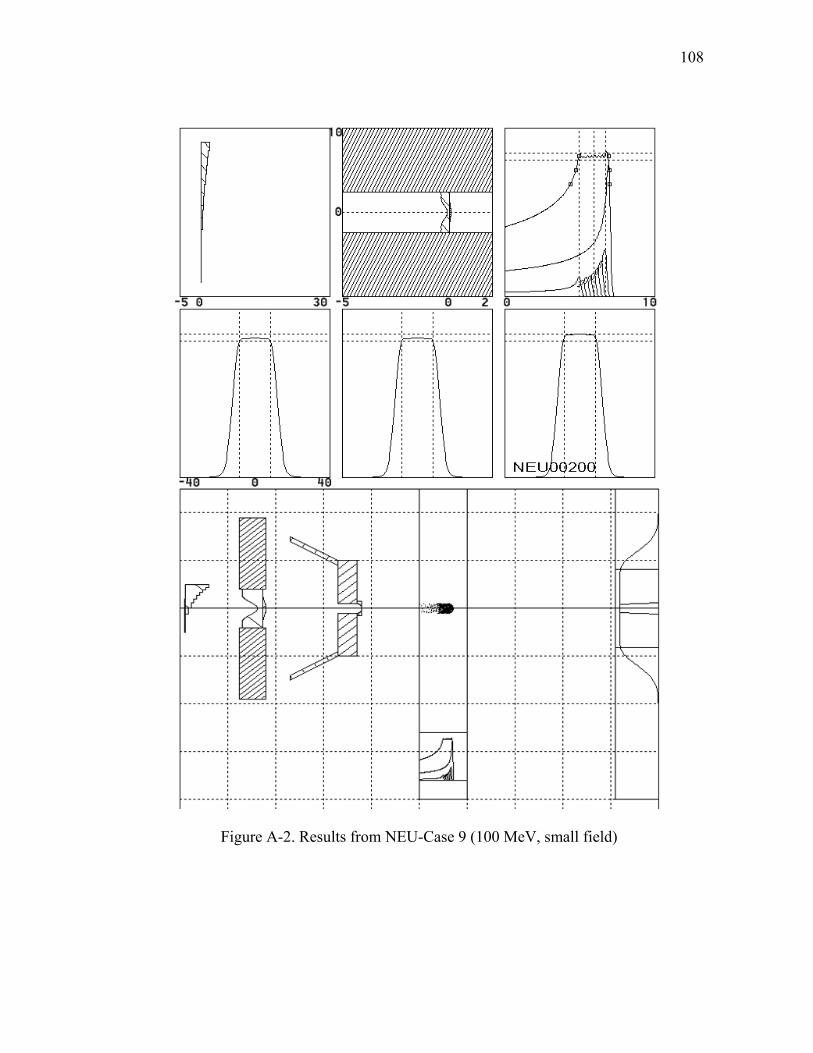
108

Figure A-2. Results from NEU-Case 9 (100 MeV, small field)

109

APPENDIX B

EXECUTION OF “MCNP_PSTUDY” AND “MERGE_MCTAL” SCRIPTS

B.1 “Mcnp_pstudy” Input File for MCNPX-Case 7

c Created on: Wednesday, August 5th, 2009 at 19:00 c beam energy H_Eng c @@@ H_Eng = 250 c s1 parameters: weight, pb and Lexan thicknesses, number of steps c @@@ No_Step = 11 c @@@ Step_Wgt = 0.4006 0.1378 0.0965 0.0739 0.0608 \ c @@@ 0.0513 0.0437 0.0379 0.0343 0.0287 0.0344 c @@@ S1_Pb = 0.8829 0.8679 0.8515 0.8344 0.8166 \ c @@@ 0.7982 0.7791 0.7593 0.7388 0.7176 0.6956 c @@@ S1_LE = 0.0001 0.9377 1.8827 2.8317 3.7842 \ c @@@ 4.7402 5.6996 6.6627 7.6294 8.6003 9.5754 c s2 parameters: radius, Lexan and pb thicknesses, shielding size c @@@ r0 = 0.001 c @@@ r1 = 0.5331 c @@@ r2 = 1.0662 c @@@ r3 = 1.5993 c @@@ r4 = 2.1324 c @@@ r5 = 2.6655 c @@@ r6 = 3.1986 c @@@ r7 = 3.7317 c @@@ r8 = 4.2648 c @@@ r9 = 4.7979 c @@@ r10 = 11.0 c @@@ t101 = 0.1002 c @@@ t102 = 0.4135 c @@@ t103 = 1.2238 c @@@ t104 = 2.2867 c @@@ t105 = 3.3258 c @@@ t106 = 4.071 c @@@ t107 = 4.4633 c @@@ t108 = 4.5001 c @@@ t109 = 4.5001 c @@@ t110 = 4.5001 c @@@ t201 = 0.8731 c @@@ t202 = 0.811 c @@@ t203 = 0.6505

110

c @@@ t204 = 0.4397 c @@@ t205 = 0.2334 c @@@ t206 = 0.0853 c @@@ t207 = 0.0073 c @@@ t208 = 0 c @@@ t209 = 0 c @@@ t210 = 0 c @@@ air101 = ( (t102 - t101) ) c @@@ air102 = ( (t103 - t102) ) c @@@ air103 = ( (t104 - t103) ) c @@@ air104 = ( (t105 - t104) ) c @@@ air105 = ( (t106 - t105) ) c @@@ air106 = ( (t107 - t106) ) c @@@ air107 = ( (t108 - t107) ) c @@@ air108 = ( (t109 - t108) ) c @@@ air109 = ( (t110 - t109) ) c @@@ pb201 = ( (t202 - t201) ) c @@@ pb202 = ( (t203 - t202) ) c @@@ pb203 = ( (t204 - t203) ) c @@@ pb204 = ( (t205 - t204) ) c @@@ pb205 = ( (t206 - t205) ) c @@@ pb206 = ( (t207 - t206) ) c @@@ pb207 = ( (t208 - t207) ) c @@@ pb208 = ( (t209 - t208) ) c @@@ pb209 = ( (t210 - t209) ) c collimators and aperture's inner size, large field c @@@ Rcoll = 12.5 c @@@ Raper = 10 c @@@ OPTIONS = -inner c @@@ OPTIONS = -mcnp 'mpirun -np 20 /usr/local/mcnpx-v26f/bin/mcnpx.mpi' c @@@ OPTIONS = -mcnp_opts 'o=1e7out' c @@@ OPTIONS = -setup c c @@@ OPTIONS = -run c c @@@ OPTIONS = -collect 1 0 1 $void 101 0 -101 $cookie cutter 201 252 -11.35 -201 $s1 compensator Pb 202 289 -1.2 -202 $s1 range modulator 301 289 -1.2 -301 311 312 313 314 315 316 317 $s2 Lexan 302 252 -11.35 -321 :-322 :-323 :-324 :-325 :-326 :-327 $s2 pb 303 290 -8.35 331 -332 $collimator brass 401 256 -1.04 -401 $range shifter, ABS resin 501 290 -8.35 -501 503 $final aperture, brass 502 256 -1.04 -504 505 $patient specific compensator, ABS

111

503 290 -8.35 -501 502 trcl=22 $2nd collimator 504 290 -8.35 -501 502 trcl=3 $3rd collimator 505 290 -8.35 -501 502 trcl=4 $4th collimator 601 244 -7.86 -602 601 $steel shell 701 280 -1 -701 $water tank 801 204 -0.001225 -1 #101 #201 #202 #301 #302 #303 #401 #501 #502 #503 #504 #505 #601 #701 $air 1 so 400 $void sphere 101 rcc -30.5 0 0 1 0 0 3 $cookie cutter 201 rcc 0 0 0 -S1_Pb 0 0 10 $s1 scattering power compensator Pb 202 rcc 0 0 0 S1_LE 0 0 10 $s1 range modulator Lexan 301 1 rcc 0 0 0 -t110 0 0 r9 $s2 Lexan outer 311 1 trc -t102 0 0 air101 0 0 r1 r0 $s2 Lexan air trunc1 312 1 trc -t103 0 0 air102 0 0 r2 r1 $s2 air trunc2 313 1 trc -t104 0 0 air103 0 0 r3 r2 314 1 trc -t105 0 0 air104 0 0 r4 r3 315 1 trc -t106 0 0 air105 0 0 r5 r4 316 1 trc -t107 0 0 air106 0 0 r6 r5 317 1 trc -t108 0 0 air107 0 0 r7 r6 c 318 1 trc -t109 0 0 air108 0 0 r8 r7 c 319 1 trc -t110 0 0 air109 0 0 r9 r8 c $s2 pb trunc 1 321 1 trc t201 0 0 pb201 0 0 r0 r1 322 1 trc t202 0 0 pb202 0 0 r1 r2 323 1 trc t203 0 0 pb203 0 0 r2 r3 324 1 trc t204 0 0 pb204 0 0 r3 r4 325 1 trc t205 0 0 pb205 0 0 r4 r5 326 1 trc t206 0 0 pb206 0 0 r5 r6 327 1 trc t207 0 0 pb207 0 0 r6 r7 c 328 1 trc t208 0 0 pb208 0 0 r7 r8 c 329 1 trc t209 0 0 pb209 0 0 r8 r9 331 1 rcc 2 0 0 -8 0 0 r9 $s2 inner shielding 332 1 rcc 2 0 0 -8 0 0 r10 $s2 outer shielding 401 2 rpp 0 1 -15 15 -15 15 $range shifter 501 5 rpp -10 0 -20 20 -20 20 $collimator outer 502 5 rpp -10 0 -Rcoll Rcoll -Rcoll Rcoll $collimator inner 503 5 rcc -10 0 0 10 0 0 Raper $aperture inner 504 5 rpp 0 Raper -18 18 -18 18 $compensator outer 505 5 so Raper $spherical compensator inner 601 rpp -35 250 -20 20 -20 20 $steel shell inner 602 rpp -40 250 -25 25 -25 25 $steel shell outer 701 rpp 300 340 -40 40 -40 40 $water tank

112

mode h imp:h 0 1 14r $ 1,801 c material cards m280 1000. -0.111915 $Water (density of 1 assumed) 8000. -0.888085 m289 1000. -0.055491 $Lexan 6000. -0.755751 8000. -0.188758 m290 29000. -0.67 $brass 30000. -0.33 m252 82000. -1 $lead m256 1000. 32 $ABS resin,(C3H3N)2:(C4H6)3:(C8H8)5 6000. 29 7000. 1 m204 7000. -0.755636 $air -0.001225 (US S. Atm at sea level) 8000. -0.231475 18000. -0.012889 m244 26000. -1 $iron (-7.86) c transformation cards c for s2 contoured second scatterer, 1st collimator *tr1 50 0 0 c for range shifter, 2nd collimator *tr2 100 0 0 *tr22 50 0 0 9j -1 c for 3rd collimator *tr3 100 0 0 9j -1 c for 4th collimator *tr4 150 0 0 9j -1 c for final aperture, patient specific compensator *tr5 250 0 0 c void some cells c void 303 401 501 502 503 504 505 601 801 $keep S1,S2 c void 401 502 $void shifter, compensator c source definition c sdef x -30 y d1 z d2 erg d3 par h vec 1 0 0 dir 1 ccc 4 wgt Step_Wgt $Gauss sdef pos -30 0 0 erg H_Eng par h vec 1 0 0 dir 1 wgt Step_Wgt $point source c sp1 -41 0.54 0 $Y position Gaussian distribution c sp2 -41 1.22 0 $Z position Gaussian distribution c sp3 -4 0.184 100 $Energy Gaussian distribution c sp3 -4 0.292 180 $Energy Gaussian distribution c sp3 -4 0.346 250 $Energy Gaussian distribution c physics settings cut:h j 20 $emin, range 4.3 mm in water phys:h 300 $emax c lca 2 1 0 5j 2 $ use incl4 model lca 2 1 0 5j 1 $ use cem03 model, spend less time than incl4 lcb 6j 1 0 $ 1 0 stand for cutoff kinetic energy and no correction

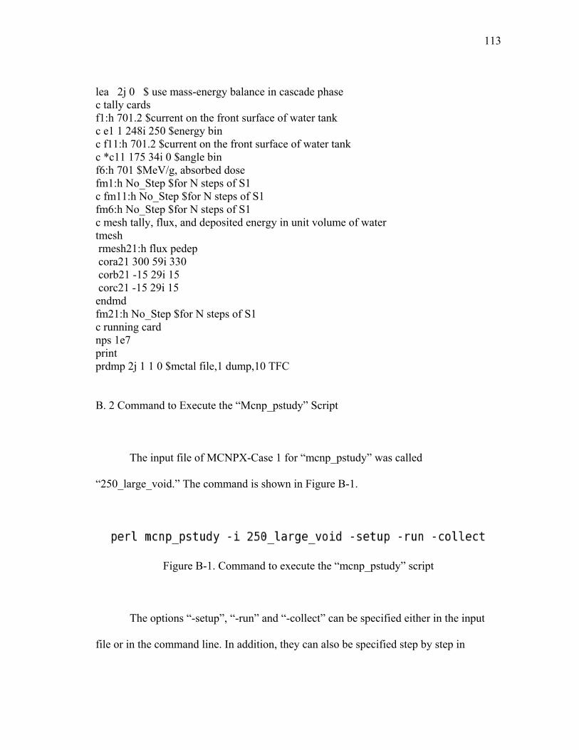
113

lea 2j 0 $ use mass-energy balance in cascade phase c tally cards f1:h 701.2 $current on the front surface of water tank c e1 1 248i 250 $energy bin c f11:h 701.2 $current on the front surface of water tank c *c11 175 34i 0 $angle bin f6:h 701 $MeV/g, absorbed dose fm1:h No_Step $for N steps of S1 c fm11:h No_Step $for N steps of S1 fm6:h No_Step $for N steps of S1 c mesh tally, flux, and deposited energy in unit volume of water tmesh rmesh21:h flux pedep cora21 300 59i 330 corb21 -15 29i 15 corc21 -15 29i 15 endmd fm21:h No_Step $for N steps of S1 c running card nps 1e7 print prdmp 2j 1 1 0 $mctal file,1 dump,10 TFC

B. 2 Command to Execute the “Mcnp_pstudy” Script

The input file of MCNPX-Case 1 for “mcnp_pstudy” was called

“250_large_void.” The command is shown in Figure B-1.

Figure B-1. Command to execute the “mcnp_pstudy” script

The options “-setup”, “-run” and “-collect” can be specified either in the input

file or in the command line. In addition, they can also be specified step by step in

114

separate command lines. Notice that the format of the input file must be a “UNIX”

format; while a “DOS” format file cannot be read in. After “-setup”, eleven sub-cases

(representing eleven steps in S1) and a log file were created in current directory, shown

in Figure B-2. After “-run”, eleven sub problems would be executed one after one, and

the output files would be created.

Figure B-2. Creation of sub-directories and files by the “mcnp_pstudy” script

B. 3 Command to Execute the “Merge_mctal” Script

In this research, a script “mergecsh” was edited to invoke the command to

execute the “merge_mctal” script. The content of “mergecsh” is shown in Figure B-3.

Figure B-3. The content of “mergecsh”

115

The modifications of the “mctal” files from MCNPX-Case 1 are shown in Figure

B-4. The original mesh tally ‘21’ was changed to an F5 tally ‘25’. The number of

meshes 6320 was kept after ‘f.’ ‘2’ after ‘s’ representing ‘flux’ and ‘pedep’ were used in

a mesh tally was kept.

Figure B-4. The modifications of the “mctal” files from MCNPX-Case 1

After modification of all the mctal files, the command “./mergecsh” was

executed on a UNIX platform; then the eleven “mctal” files were merged to one “mctal”

file - “250_l_void” in the current directory. The procedure is shown in Figure B-5.

116

Figure B-5. The execution and print-out information from “mergecsh”

117

APPENDIX C

MCNPX PLOT COMMANDS USED IN THIS RESEARCH

C.1 Commands for Energy and Angular Distribution Spectra in MCNPX-Case 1, 2 and 3

mcnpx z rmctal mctal tal 1 free e nonorm plinear tal 11 free c

C.2 Commands for Fluence and Dose Distributions in MCNPX-Case 1, 2 and 3

mcnpx z rmctal mctal tal 21 free i fixed j 1 fixed k 40 fixed s 1 nonorm plinear fixed s 2 linlin plinear tal 21 free ik fixed s 1 tal 21 free ik fixed s 2

C.3 Commands for Fluence and Dose Distributions in MCNPX-Case 4 through 15

The commands for MCNPX-Case 4 are listed below. In other cases, only the

indexes of i, j and k are different. The indexes of i can be found in Table C-1.

mcnpx z rmctal mctal tal 21 free ij fixed k 15 fixed s 1 fixed s 2 tal 21 free I fixed j 15 fixed k 15 fixed s 1 nonorm plinear fixed s 2 tal 21 free jk fixed i 1 fixed s 1 fixed i 30

118

fixed i 1 fixed s 2 fixed i 30 tal 21 free j fixed k 15 fixed i 30 fixed s 1 fixed i 40 fixed i 50 tal 21 free j fixed k 15 fixed s 2 fixed i 30 fixed i 40 fixed i 50

Table C-1. Coordinate or Index of i in the mesh tally for transverse dose distribution

MCNPX-Case No.

Coordinate or Index

Proximal point at SOBP

Middle point at SOBP

Distal point at SOBP

X (cm) 316 321 326 1 Index of i 32 42 52 X (cm) 320 325 330 2 Index of i 40 50 60 X (cm) 324 329 334 3 Index of i 48 58 68 X (cm) 315 320 325 4 Index of i 30 40 50 X (cm) 320 325 330 5 Index of i 40 50 60 X (cm) 324 329 334 6 Index of i 48 58 68 X (cm) 314 319 324 7 Index of i 28 38 48 X (cm) 319 324 329 8 Index of i 38 48 58 X (cm) 323 328 333 9 Index of i 46 56 66 X (cm) 306 310 314 10 Index of i 12 20 28 X (cm) 308 312 316 11 Index of i 16 24 32 X (cm) 311 315 319 12 Index of i 22 30 38 X (cm) 302.5 303.5 304.5 13 Index of i 5 7 9 X (cm) 303 304 305 14 Index of i 6 8 10 X (cm) 303.5 304.5 305.5 15 Index of i 7 9 11

119

VITA

Name: Fada Guan

Address: 3133 TAMU, Department of Nuclear Engineering,

College Station, TX, USA, 77843-3133

Email address: guanfada@tamu.edu, guanfada@gmail.com

Education: B.E., Nuclear Engineering and Nuclear Technique,

Tsinghua University, China, 2005