Embed Size (px)
Citation preview
Candidate
Susana Patrícia Oliveira Mendonça
Novembro 2015
Protocol optimization for the ultrastructural preservation
of cilia in Drosophila melanogaster’s antenna
THESIS TO OBTAIN THE MASTER OF SCIENCE DEGREE IN
BIOMEDICAL TECHNOLOGIES
Supervisors
Dr. Raúl Daniel Lavado Carneiro Martins
(Professor of the Bioengineering Department at Instituto Superior Técnico)
Dra. Erin Marie Tranfield
(Head of the Electron Microscopy Facility in Instituto Gulbenkian de Ciência)
Examination Committee
Chairperson: Prof. Maria Margarida Fonseca Rodrigues Diogo
Supervisor: Dra. Erin Marie Tranfield
Members of the Committee: Dra. Maria João Lopes Gonçalves de Brito Amorim
ii
Acknowledgments
I would like to express my gratitude towards my supervisors Dra. Erin Tranfield and Dr. Raúl
Martins for their advices and for leading me into the right direction in this project. Also, towards my
group leader, Dra. Mónica Bettencourt-Dias for allowing me to conduct my experiments on my
workplace and for all the inputs she has given me on what to focus my research on.
As well, I have to thank my colleagues from the Cell Cycle Regulation Lab for the suggestions
regarding the organization of my experiments, especially to Pedro Machado and Swadhin Jana who
started the protocol optimization that gave rise to this project.
Also, I want to thank my colleagues from the Electron Microscopy facility for their help with
some technical work.
Last but not the least, a big thank you for my family and friends for all the moral support they
have given me, because without all of them this work could not be accomplished.
iii
Glossary
% – Percentage
ºC – Degrees Celsius
ChF – Chemical fixation
CrF – Cryo fixation
Dm – Drosophila melanogaster
EM – Electron Microscopy
FM – Formaldehyde
FS – Freeze substitution
Glut – Glutaraldehyde
HPF – High pressure freezing
MT – Microtubules
IPE – Individual Protection Equipment
LC – Lead citrate
OsO4 – Osmium tetroxide
PBS – Phosphate Buffered Saline
PHEM – Pipes – HEPES- EGTA – MgCl2
RT – Room Temperature
TEM – Transmission Electron Microscope
UA – Uranyl Acetate
iv
Contents
Acknowledgments ........................................................................................................................ ii
Glossary ...................................................................................................................................... iii
Contents ..................................................................................................................................... iv
List of tables .............................................................................................................................. viii
List of figures ............................................................................................................................ viii
Abstract ........................................................................................................................................x
Resumo....................................................................................................................................... xi
1. Introduction .......................................................................................................................... 1
1.1 Motivation ......................................................................................................................... 1
1.2 Questions to start with ...................................................................................................... 1
1.3 Goals ................................................................................................................................ 1
1.4 Strategies to answer the questions .................................................................................. 2
1.5 Hypothesis ........................................................................................................................ 2
1.6 Thesis outline .................................................................................................................... 3
2. Transmission Electron Microscopy ...................................................................................... 4
2.1 Historical Context .............................................................................................................. 4
2.1.1 Conventional fixation ................................................................................................. 5
2.1.2 Cryofixation ................................................................................................................ 6
2.1.3 High pressure freezing .............................................................................................. 6
3. Traditional techniques for specimen preparation ................................................................ 7
3.1 Chemical fixation .............................................................................................................. 7
3.1.1 Aldehydes .................................................................................................................. 9
3.1.2 Osmium tetroxide (OsO4) ........................................................................................ 10
3.1.3 Fixative vehicle ........................................................................................................ 11
3.1.4 Effects of chemical fixation ...................................................................................... 17
4. Cryo techniques for specimen preparation ........................................................................ 22
4.1 High Pressure Freezing .................................................................................................. 22
4.2 Physics of ice formation in biological specimens ........................................................... 23
4.2.1 Technology of high pressure freezing ..................................................................... 25
4.3 Freeze substitution ......................................................................................................... 26

v
5. Cilia .................................................................................................................................... 27
5.1 Drosophila melanogaster ................................................................................................ 28
5.2 Electron Microscopy in the antenna of Drosophila melanogaster .................................. 29
6. Methodology ...................................................................................................................... 31
6.2 Sampling and sample ..................................................................................................... 31
6.3 Lab work ......................................................................................................................... 32
6.4 Methods for chemical fixation ......................................................................................... 32
6.4.1 Sample processing solutions ................................................................................... 32
6.4.2 Chemical Fixation Protocol ...................................................................................... 33
6.4.3 Randomization of samples ...................................................................................... 34
6.4.4 Sample selection and sectioning ............................................................................. 34
6.4.5 Sample post-staining ............................................................................................... 35
6.4.6 Sample imaging ....................................................................................................... 35
6.4.7 Sample evaluation ................................................................................................ 36
6.4.8 Statistical analysis ................................................................................................... 39
6.5 Methods for cryo fixation ........................................................................................... 39
6.5.1 Sample processing solutions ................................................................................... 39
6.5.2 Cryo Fixation Protocol ............................................................................................. 40
6.5.3 Randomization of samples ...................................................................................... 41
6.5.4 Sample selection and sectioning ............................................................................. 41
6.5.5 Sample post-staining ............................................................................................... 41
6.5.6 Sample imaging ....................................................................................................... 41
6.5.7 Sample evaluation ................................................................................................ 41
6.5.8 Statistical analysis ................................................................................................ 41
6.6 Materials, Reagents, Equipment and IPE ...................................................................... 41
7. Results ............................................................................................................................... 42
7.1 Chemical fixation results ................................................................................................. 42
7.1.1Evaluation chart with the buffer scores .................................................................... 42
7.1.2 Sample scoring by different evaluators ................................................................... 42
7.1.3 Buffer final evaluation scores .................................................................................. 42
7.1.4 General evaluation scores ....................................................................................... 43

vi
7.1.5 Cilia evaluation scores ............................................................................................. 44
7.1.6 Panel Analysis ......................................................................................................... 44
7.2 Cryo fixation results ........................................................................................................ 46
7.2.1 Evaluation chart with the buffer scores ................................................................... 46
7.2.2 Freeze substitution final evaluation scores ............................................................. 46
7.2.3 General evaluation scores ....................................................................................... 46
7.2.4 Cilia evaluation scores ............................................................................................. 47
7.2.5 Panel Analysis ......................................................................................................... 47
7.3 Chemical vs Cryo fixation ............................................................................................... 48
7.3.1 Comparison of the general score between the best and worst buffer and the best
and worst freeze substitution protocol ........................................................................................... 48
7.3.2 Comparison of the cilia score between the best and worst buffer and the best and
worst freeze substitution protocol .................................................................................................. 48
8. Discussion and Conclusion ............................................................................................... 49
9. References ........................................................................................................................... 56
10. Appendix ............................................................................................................................. 62
10.1 Quantitative evaluation of the samples chemically fixed using the criteria for judging
ultrastructure quality .......................................................................................................................... 62
10.2 Quantitative evaluation of the samples cryo fixed using the criteria for judging
ultrastructure quality .......................................................................................................................... 64
10.3 Quantitative evaluation of the samples by different evaluators using the criteria for
judging ultrastructure quality ............................................................................................................. 65
10.4 Chemical Fixation Panels ............................................................................................. 66
10.4.1 Schematic Representation on how the panels are organized ............................... 66
10.4.3 Phosphate Sample 1b ........................................................................................... 67
10.4.4 Phosphate Sample 1c ........................................................................................... 67
10.4.5 PHEM Sample 1a .................................................................................................. 68
10.4.6 PHEM Sample 1b .................................................................................................. 68
10.4.7 PHEM Sample 1c .................................................................................................. 69
10.4.8 Cacodylate Sample 1a .......................................................................................... 69
10.4.9 Cacodylate Sample 1b .......................................................................................... 70
10.4.10 Cacodylate Sample 1c ......................................................................................... 70
10.4.11 PBS Sample 1a ................................................................................................... 71

vii
10.4.12 PBS Sample 1b ................................................................................................... 71
10.4.13 PBS Sample 1c.................................................................................................... 72
10.4.14 Water Sample 1a ................................................................................................. 72
10.4.15 Water Sample 1b ................................................................................................. 73
10.4.16 Water Sample 1c ................................................................................................. 73
10.4.17 Phosphate Sample 2 ........................................................................................... 74
10.4.18 PHEM Sample 2 .................................................................................................. 74
10.4.19 Cacodylate Sample 2 .......................................................................................... 75
10.4.20 PBS Sample 2 ..................................................................................................... 75
10.4.21 Water Sample 2 ................................................................................................... 76
10.4.22 Phosphate Sample 3 ........................................................................................... 76
10.4.23 PHEM Sample 3 .................................................................................................. 77
10.4.24 Cacodylate Sample 3 .......................................................................................... 77
10.4.25 PBS Sample 3 ..................................................................................................... 78
10.4.26 Water Sample 3 ................................................................................................... 78
10.5 Cryo Fixation Panels..................................................................................................... 79
10.5.1 Fast Freeze Substitution Sample 1 ....................................................................... 79
10.5.2 Fast Freeze Substitution Sample 2 ....................................................................... 79
10.5.3 Medium Freeze Substitution Sample 1.................................................................. 80
10.5.4 Medium Freeze Substitution Sample 2.................................................................. 80
10.5.5 Slow Freeze Substitution Sample 1....................................................................... 81
10.5.6 Slow Freeze Substitution Sample 2....................................................................... 81
10.6 Materials, Reagents and Individual Protection Equipment ........................................... 82

viii
List of tables
TABLE 1: A STANDARD TISSUE PREPARATION SCHEME TO PROCESS BIOLOGICAL SAMPLES FOR ELECTRON MICROSCOPY. ORIGINALLY DAPTED FROM (BOZZOLA & RUSSEL, 1999)………….……….……… 8 TABLE 2: SUMMARY OF SOME FIXATIVE CHARACTERISTICS……………………………………………………….…… 11 TABLE 3: SUMMARY OF BUFFER RANGE AT 25ºC OF THE DIFFERENT USED BUFFERS………….………….. 17 TABLE 4: SAMPLE DIVISION FOR CHEMICAL PROCESSING ACCORDING TO EACH ANALYZED BUFFER. …………………………………………………………………………………………………………………………………………………………31 TABLE 5: SAMPLE DIVISION FOR CRYO PROCESSING ACCORDING TO EACH PARAMETER TO ANALYZE. …………………………………………………………………………………………………………………………………………….…………..31 TABLE 6: SCHEMATIC OF HOW THE SECTIONING WAS DONE FOR SAMPLES 1A, 1B AND 1C….……….. 34 TABLE 7: SUMMARY OF THE PICTURES NEEDED TO USE THE TABLE FOR EVALUATION………….……….. 35 TABLE 8: CLASSIFICATION TABLE FOR THE EVALUATION OF THE GENERAL FEATURES OF THE SAMPLES……………………………………………………………………………………………………………………………….……….. 38 TABLE 9: CLASSIFICATION TABLE FOR THE EVALUATION OF THE CILIARY FEATURES OF THE SAMPLES. …………………………………………………………………………………………………………………………………………………………39
List of figures
FIG. 1: FORMALDEHYDE MOLECULE. SOURCE:
HTTP://WWW.AMMRF.ORG.AU/MYSCOPE/TEM/PRACTICE/PREP/FIXATION/ .............................................. 9
FIG. 2: GLUTARALDEHYDE MOLECULE. SOURCE:
HTTP://WWW.AMMRF.ORG.AU/MYSCOPE/TEM/PRACTICE/PREP/FIXATION/ .............................................. 9
FIG. 3: OSMIUM TETROXIDE MOLECULE. SOURCE: HTTP://COMMONS.WIKIMEDIA.ORG/WIKI/FILE:OSMIUM-
TETROXIDE-2D-STRUCTURAL.PNG ................................................................................................................ 10
FIG. 4: THEORETICAL PLOT OF PH VERSUS [A-]/[HA] ON TWO-CYCLE SEMILOG PAPER (MOHAN, 2003). ........ 14
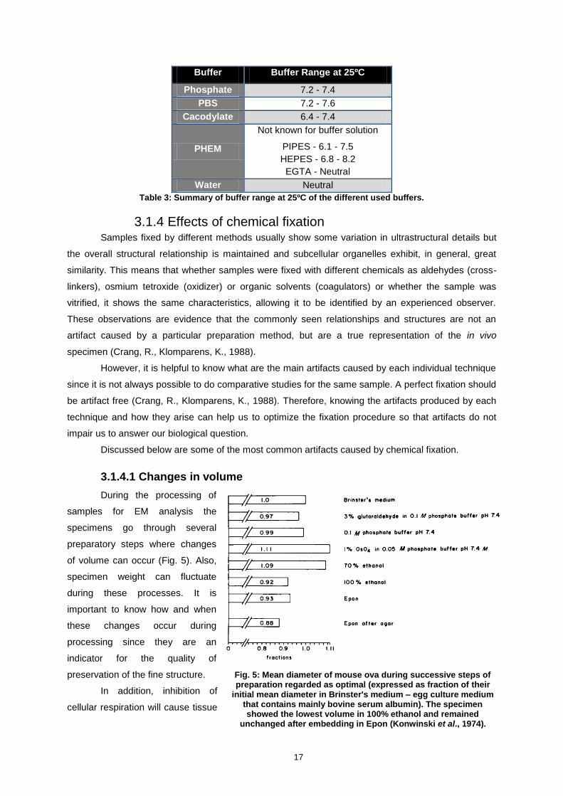
FIG. 5: MEAN DIAMETER OF MOUSE OVA DURING SUCCESSIVE STEPS OF PREPARATION REGARDED AS OPTIMAL
(EXPRESSED AS FRACTION OF THEIR INITIAL MEAN DIAMETER IN BRINSTER'S MEDIUM – EGG CULTURE
MEDIUM THAT CONTAINS MAINLY BOVINE SERUM ALBUMIN). THE SPECIMEN SHOWED THE LOWEST
VOLUME IN 100% ETHANOL AND REMAINED UNCHANGED AFTER EMBEDDING IN EPON (KONWINSKI ET
AL., 1974). ..................................................................................................................................................... 17
FIG. 6: HOMOGENEOUS NUCLEATION (TH) AND EQUILIBRIUM MELTING TEMPERATURES (TM) FOR WATER IN
EMULSION FORM AS A FUNCTION OF PRESSURE. THE DASHED, VERTICAL LINE INDICATES THE
CONDITIONS UNDER WHICH ICE II AND ICE III MAY BE PRODUCED IN HIGH PRESSURE FROZEN SAMPLES
(ADAPTED FROM KANNO ET AL, 1975). ........................................................................................................ 24
FIG. 7: RECORD OF PRESSURE (PURPLE LINE) AND TEMPERATURE (YELLOW LINE) CHANGES DURING FREEZING
(TOTAL TIME = ~380 MS) IN THE WOHLWEND COMPACT 02 HIGH PRESSURE FREEZING MACHINE.
TEMPERATURE DROPS APPROXIMATELY -120ºC. ......................................................................................... 25
FIG. 8: SCHEMATIC REPRESENTATION OF A LONGITUDINAL VIEW OF THE CILIUM AND ITS COMPARTMENTS.
(JANA ET AL, 2014). ....................................................................................................................................... 27
FIG. 9: SCHEMATIC REPRESENTATION OF THE HEAD OF DROSOPHILA MELANOGASTER. THE INSET SHOWS ONE
OF THE TWO ANTENNAE THAT ARE POSITIONED BETWEEN THE EYES OF THE FLY. IN THE INSET THE

ix
SEVERAL SEGMENTS OF THE ANTENNA ARE REPRESENTED AS WELL AS THE ARISTA, ANOTHER SENSORY
ORGAN. ......................................................................................................................................................... 28
FIG. 10: SCHEMATIC REPRESENTATION OF AN OLFACTORY CILIUM. A) LONGITUDINAL SCHEME OF OLFACTORY
CILIUM. THE ARROW REPRESENTS THE TRANSITION ZONE AREA. B) CROSS SECTION REPRESENTATION OF
THE TRANSITION ZONE. C) SCHEMATIC REPRESENTATION OF THE Y-LINKER STRUCTURES (DARK GREY)
CONNECTING THE MICROTUBULES (GREEN CIRCLES WITH A AND B) TO THE MEMBRANE (BROWN). (JANA,
S. UNPUBLISHED) .......................................................................................................................................... 29
FIG. 11: ANATOMY OF OLFACTORY CILIUM (JANA, 2011).................................................................................... 30
FIG. 12: LOW-MAGNIFICATION VIEWS OF EPIDERMAL CELLS PROCESSED BY HPF-FS (A) OR CONVENTIONAL
FIXATION (B). SCALE BARS, 1 ΜM (MCDONALD, 2014). ............................................................................... 30
FIG. 13: GRAPHIC REPRESENTING THE FINAL SCORE OF THE SAMPLES ANALYZED BY FOUR INDEPENDENT
EVALUATOR (CREATOR OF THE TABLE, AN ELECTRON MICROSCOPY EXPERT, A BIOLOGIST AND AN AIR
TRAFFIC CONTROLLER) TO ASSESS EVALUATION TABLE UTILITY. ................................................................. 42
FIG. 14: GRAPHIC REPRESENTING THE FINAL EVALUATION SCORE OF THE SAMPLES ANALYZED FOR THE FIVE
DIFFERENT BUFFERS USED IN THE CHEMICAL FIXATION PROTOCOL............................................................ 43
FIG. 15: GRAPHIC REPRESENTING THE GENERAL EVALUATION SCORE OF THE SAMPLES ANALYZED FOR THE FIVE
DIFFERENT BUFFERS USED IN THE CHEMICAL FIXATION PROTOCOL............................................................ 43
FIG. 16: GRAPHIC REPRESENTING THE CILIA EVALUATION SCORE OF THE SAMPLES ANALYZED FOR THE FIVE
DIFFERENT BUFFERS USED IN THE CHEMICAL FIXATION PROTOCOL............................................................ 44
FIG. 17: PICTURES REPRESENTING THE BEST AND WORST CILIA SCORES FOR ALL THE DIFFERENT BUFFERS
ANALYZED IN THE CHEMICAL FIXATION PROTOCOL. SCALE BARS REPRESENT 500NM. ............................... 45
FIG. 18: GRAPHIC REPRESENTING THE FINAL EVALUATION SCORE OF THE SAMPLES ANALYZED FOR THE THREE
DIFFERENT FREEZE SUBSTITUTION TIMES USED IN THE CRYO FIXATION PROTOCOL................................... 46
FIG. 19: GRAPHIC REPRESENTING THE GENERAL EVALUATION SCORE OF THE SAMPLES ANALYZED FOR THE
THREE DIFFERENT FREEZE SUBSTITUTION TIMES USED IN THE CRYO FIXATION PROTOCOL. ...................... 46
FIG. 21: PICTURES REPRESENTING OF THE BEST AND WORST SCORES FOR ALL THE FREEZE SUBSTITUTION TIMES
ANALYZED IN THE CRYO FIXATION PROTOCOL. SCALE BARS REPRESENT 500NM. ....................................... 47
FIG. 20: GRAPHIC REPRESENTING THE CILIA EVALUATION SCORE OF THE SAMPLES ANALYZED FOR THE THREE
DIFFERENT FREEZE SUBSTITUTION TIMES USED IN THE CRYO FIXATION PROTOCOL................................... 47
FIG. 22: ON THE LEFT: REPRESENTATIVE GRAPHIC OF THE BEST AND WORSE SCORES IN THE GENERAL
EVALUATION FOR THE SAMPLES ANALYZED FOR CHEMICAL AND CRYO FIXATION. ON THE RIGHT: PICTURES
REPRESENTATIVE OF THE VALUES OF THE GENERAL SCORE FROM THE SAMPLES REPRESENTED IN THE
PANEL. SCALE BARS REPRESENT 500NM. ...................................................................................................... 48
FIG. 23: ON THE LEFT: REPRESENTATIVE GRAPHIC OF THE BEST AND WORSE SCORES IN THE CILIA EVALUATION
FOR THE SAMPLES ANALYZED FOR CHEMICAL AND CRYO FIXATION. ON THE RIGHT: PICTURES
REPRESENTATIVE OF THE VALUES OF THE CILIA SCORE FROM THE SAMPLES REPRESENTED IN THE PANEL.
SCALE BARS REPRESENT 500NM. .................................................................................................................. 48

x
Abstract
Cilia are microtubule-based organelles involved in a variety of processes, such as sensing,
motility and cellular architecture-organizing functions. Moreover, they are altered in several human
conditions called ciliopathies and are involved in cancer.
To understand these pathologies, a detailed knowledge of the biology of cilia is required.
These organelles are remarkably well conserved throughout eukaryotic evolution and have been well
studied in Drosophila melanogaster (Dm).
Dm is an advantageous model organism to study several biological and physiological
properties since they are conserved between the fly and mammals, and nearly 75% of human
disease-causing genes are believed to have a functional homolog in the fly. Other advantages are the
availability of powerful genetics tools, highly conserved disease pathways, very low comparative costs,
rapid life cycle and no ethical problems.
Despite these advantages, there is still a gap in the application of transmission electron
microscopy (TEM) to study the ultrastructure of Dm. One of the reasons is the difficult-to-process
chitin exoskeleton that surrounds the fly body, in particular the antenna, an organ that contains ciliated
neurons. Also, basic sample preparation procedures for resin embedding of biological specimens have
not evolved much since the 1960’s and newer methods such as cryo techniques have not been used
to study this organ.
Therefore, the goal of this project is to develop an optimized TEM protocol, both for chemical
and cryo processing in the antenna of Dm, which can help to provide the necessary leap to expand
the utilization of this model in research.
KEY-WORDS: Ultrastructure, protocol optimization, cilia, Drosophila melanogaster, chemical
fixation, cryo fixation.
xi
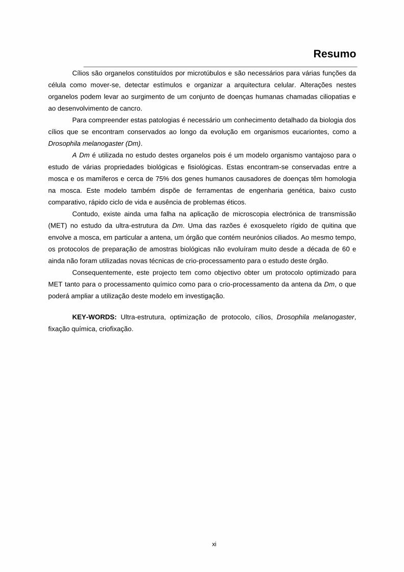
Resumo
Cílios são organelos constituídos por microtúbulos e são necessários para várias funções da
célula como mover-se, detectar estímulos e organizar a arquitectura celular. Alterações nestes
organelos podem levar ao surgimento de um conjunto de doenças humanas chamadas ciliopatias e
ao desenvolvimento de cancro.
Para compreender estas patologias é necessário um conhecimento detalhado da biologia dos
cílios que se encontram conservados ao longo da evolução em organismos eucariontes, como a
Drosophila melanogaster (Dm).
A Dm é utilizada no estudo destes organelos pois é um modelo organismo vantajoso para o
estudo de várias propriedades biológicas e fisiológicas. Estas encontram-se conservadas entre a
mosca e os mamíferos e cerca de 75% dos genes humanos causadores de doenças têm homologia
na mosca. Este modelo também dispõe de ferramentas de engenharia genética, baixo custo
comparativo, rápido ciclo de vida e ausência de problemas éticos.
Contudo, existe ainda uma falha na aplicação de microscopia electrónica de transmissão
(MET) no estudo da ultra-estrutura da Dm. Uma das razões é exosqueleto rígido de quitina que
envolve a mosca, em particular a antena, um órgão que contém neurónios ciliados. Ao mesmo tempo,
os protocolos de preparação de amostras biológicas não evoluíram muito desde a década de 60 e
ainda não foram utilizadas novas técnicas de crio-processamento para o estudo deste órgão.
Consequentemente, este projecto tem como objectivo obter um protocolo optimizado para
MET tanto para o processamento químico como para o crio-processamento da antena da Dm, o que
poderá ampliar a utilização deste modelo em investigação.
KEY-WORDS: Ultra-estrutura, optimização de protocolo, cílios, Drosophila melanogaster,
fixação química, criofixação.

1
1. Introduction
1.1 Motivation
Most methods for processing tissue and analyzing its ultrastructure have not progressed much
since their first development in the 1960s. However, since 1960 there has been an increase in tools
that can be used to study different model organisms, such as high pressure freezing. One very
important model organism currently used in research is Drosophila melanogaster (Dm). There is
therefore a need for the electron microscopy protocols to be developed so these tools can be used as
a complementary or standalone tool in research.
Currently working in a laboratory that focus its research on cilia and centrioles, where Dm is
used as a model organism and working as an electron microscopy (EM) technician, I have seen
firsthand the need and importance to combine these two fields using a standard and optimized
protocol for the ultrastructural preservation of Dm’s antenna.
To do so, this study will focus on a more classical approach of EM, chemical fixation (ChF)
and on a more recent technology for optimized ultrastructural preservation, cryo fixation (CrF).
1.2 Questions to start with
As a first approach to this study it is necessary to think about the factors of specimen
preparation that influence the ultrastructural preservation of a tissue. There are some questions that
need to be taken into consideration for this study that should be evaluated and answered:
Does the buffer in which the fixative is suspended affect the quality of sample
preservation?
If there is a difference in quality between buffers; what are the differences?
How can the ultrastructural preservation of a tissue be quantitatively evaluated?
Can different durations of the freeze substitution (FS) procedure used on high
pressure frozen samples influence ultrastructural preservation?
Are there any differences between the best chemically fixed samples and the best
cryo processed samples?
Can two different techniques (chemical processing and cryo processing) be compared
in a quantitative way?
1.3 Goals
Taking into consideration the questions listed above, the general goal of this project was to
create an optimized protocol for chemical and cryo processing that preserves the ultrastructure of the
antenna of Dm.
The specific goals designed for this works are 1) to create a standardized protocol to fix the
antenna of Dm as close as possible to its native state by minimizing fixation artifacts both by chemical
and cryo techniques; 2) to compare the preservation quality of the antenna attained by different
2
processing strategies; 3) to create a quantitative tool to assess the quality of ultrastructural sample
preservation that also allows quantitative comparisons between samples and protocols.
1.4 Strategies to answer the questions
The strategies were adapted for the different protocols, accordingly to the properties of each
type of fixation.
For chemical processing:
Compare ultrastructural preservation quality of samples processed using a standard
fixative for electron microscopy – a modified Karnovsky’s fixative - in different buffers
(Phosphate, Cacodylate, PHEM, PBS and Water).
For cryo processing:
o Compare ultrastructural preservation quality of cryo-immobilized samples processed
using freeze substitution protocols of different durations (short – 8 hours; medium – 24
hours; and long – 52 hours).
For quantitative analysis:
o Review the literature to assess the major criteria to define ultrastructural quality for
electron microscopy samples and create a table that uses those criteria to
quantitatively grade the ultrastructural preservation of the sample.
1.5 Hypothesis
Different buffers have been used in electron microscopy for several decades but little has
been published regarding their contribution to tissue preservation and comparative studies between
them are scarce. Although some uses are known for Phosphate, PBS and Cacodylate buffers, the
action of PHEM buffer remains a topic to be studied.
In terms of general preservation, based on the convention in the field Phosphate is described
to be the best buffer for electron microscopy followed by Cacodylate buffer. Also, Phosphate is less
expensive and less toxic than Cacodylate (Bozzola & Russel, 1999). Hence, Phosphate buffer should
offer a good preservation of the ultrastructure of Dm at a lower cost.
The PHEM buffer was first developed for preserving microtubules, therefore it is expected to
give the best preservation of the antenna cells that contains cilia, a microtubule based structure that is
my structure of interest (Schilwa & Blerkom, 1981). This buffer also seems to be an ideal candidate for
regular usage because it is an organic buffer. Organic buffers show fewer detrimental effects on fine
cell structure and are nontoxic (Kuo, 2014).
Fast cryo techniques (rapid freeze substitution protocols) have been shown to give good
results for the processing of Dm samples and since faster freeze substitutions are less costly (less
amount of reagents, less instrument usage and less technician time) this should be the best choice for
cryo processing the antenna samples (Shanbhag, 1999; Shanbhag, 2000; McDonald, 2014). It has
also been shown that cryo techniques improve the tissue quality when compared to chemical
techniques (Shanbhag, 1999; Shanbhag, 2000; McDonald, 2012).

3
1.6 Thesis outline
This thesis is comprised of 10 chapters. Chapter 1 introduces the reader to the motivation
behind this work, the thesis goals and the general hypothesis driving the work. Chapter 2 reviews the
basic concepts and history of electron microscopy. Chapter 3 is dedicated to the traditional techniques
for specimen preparation while Chapter 4 focuses on cryo techniques for specimen preparation. In
Chapter 5 there is a brief explanation about cilia and Dm. Chapter 6 details the methodology used to
develop this work. Chapter 7 will present all the results, followed by its discussion and conclusion in
Chapter 8. Chapter 9 contains the references and Chapter 10 contains the appendices.

4
2. Transmission Electron Microscopy
Transmission electron microscopy (TEM) has proven to be crucial in research. However like
all microscopy techniques TEM is not perfect. Accelerated electrons propagate only under a high
vacuum environment, where water evaporates, which is a hitch in the TEM technique since biological
samples contain liquid water. As a consequence, for a sample to be imaged under vacuum it must
have all the water removed from it (Studer, 2008).
Furthermore, the electron beam can only penetrate thin structures (Hayat, 2000). In the
standard procedure, biological samples are fixed with a cocktail of aldehydes and osmium tetroxide
(OsO4), dehydrated to remove the water, embedded into a hard resin that works as a support to the
tissue, and ultra-thin sections are cut and stained with heavy metal ions (Luft, 1961). The contrast
seen in classical EM micrographs is based on differential adsorption of heavy metal cations to various
sample components rather than to the biological structures themselves. Heavy metals are added
during sample processing with osmium tetroxide fixation and uranyl acetate (UA) en block staining and
if needed during an additional step of post-staining (Hayat, 2000).
However, all preparation steps can introduce artifacts. Fixation with glutaraldehyde and
dehydration with organic solvents leads, for example, to aggregation of proteins, collapse of highly
hydrated glycans, and loss of lipids (Cope, 1968; Cope 1969 and Kellenberger, 1992).
Although some artifacts might be introduced with this technique, it was thanks to the much
higher resolution than the one achieved with a light microscope, that many cellular organelles and
substructures were first discovered by TEM (Palade, 1954). This resolution is achieved thanks to the
small wavelength of an electron and it can be expressed by the Rayleigh criterion:
ρ = 0.6λ/(n.sinμ)= 0.6λ/NA (2.1)
ρ - resolution, λ - wavelength, n - refractive index, μ - semi-angle at the specimen and NA - numerical
aperture (Egerton, 2005).
Thus, although in theory atomic resolution is possible with the electron microscope (and in
practice with inorganic samples), in practice the preparation and imaging artifacts limit the effective
resolution for biological specimens for TEM to about 2 nm (Hayat, 2000; Batson, 2002; Studer, 2008).
2.1 Historical Context
Max Knoll and Ernst Ruska invented the electron microscope in 1931 at the Berlin Technische
Hochschule. This breakthrough surpassed the limitations of visible light yielding higher resolution
microscopy. This new technique of electron microscopy allowed, for the first time, the visualization of
viruses, DNA and many smaller organelles (Egerton, 2005).
There are two basic types of electron microscopes: transmission and scanning. The
transmission electron microscope (TEM) projects electrons that pass through a thin section of tissue
(sample) and interact with it. A two-dimensional picture is produced where the brightness of an area is
proportional to the number of electrons that are transmitted through the sample. The scanning electron
microscope (SEM) uses electrons to scan the surface of the sample that give rise to secondary
electrons. These are captured by a detector and the image is produced over time, as the sample is

5
scanned. A picture of the sample’s surface is produced with a three-dimensional look (Bozzola &
Russel, 1999).
The development of the electron microscope drove the evolution of the techniques used in
microscopy. However, since the first electron microscopists where physicists and engineers, the first
applications for this type of microscope where focused on material sciences. Only afterwards, in the
1950’s, the tissue preparation techniques evolve, allowing the biological sciences to profit with the
usage of this equipment. At first, chemical fixation (ChF) was conventionally used in EM and with the
development of the techniques and the machines used, cryo fixation (CrF) techniques were employed
to try to decrease some of the artifacts caused by ChF and to help achieve a more close to native
state of the final preserved EM sample (Bozzola & Russel, 1999).
2.1.1 Conventional fixation Most of the first micrographs acquired by TEM were not much better than a light microscopy
picture. Despite the fact that the first focus of TEM analysis was applied to material sciences, it led
researchers to consider the possibility of applying it to biological sciences. This new application would
allow acquiring information regarding some small size cell components that could not be achieved with
light microscopy, such as viruses, small organelles as endoplasmic reticulum and cytoskeleton
elements.
One of the limitations to TEM application in biological samples was that specimens being
observed (like tissues and whole mounts) where too thick. It was necessary to develop a way to
section these samples into thinner slices. Although the problem was straightforward, it took some time
to develop a technique for sample sectioning. Initially in the 1950’s Hartmann employed glass knives
to acquire thin sections. This was followed by the usage of diamond knives introduced by Fernandez-
Moran (Latta & Hartmann, 1950; Fernandez-Moran, 1953).
Furthermore, to achieve the desired thin sections thickness an embedding medium to serve as
a support was needed, as well as a suitable microtome for the newly developed knives. Moreover, to
preserve the samples a good fixative was needed. A landmark in fixation was the development of
buffered osmium tetroxide fixative known as “Palade’s pickle” that was used until the mid 1960’s when
double fixation with glutaraldehyde and osmium tetroxide became the new standard fixation (Palade,
1952; Sabatini, 1963).
Until today, this fixation method continues to be used by many laboratories. Usually, the first
fixation is with formaldehyde (sometimes in a cocktail with glutaraldehyde, known as Karnovsky’s
fixative) and lasts about one hour after which a rinse with buffer is done. It is followed by a post-
fixation with osmium tetroxide for about another hour after which a rinse with buffer and/or water prior
to dehydration in an alcohol or acetone series. After these steps, the sample is infiltrated in resin and
embedded. En bloc fixation/staining with uranyl acetate has also become common practice in
conventional electron microscopy, which is usually done after the double fixation (McDonald, 2014).
This is the essence of a double fixation protocol but many variations to this can be made
regarding concentrations, buffer composition, timing, pH and so forth, accordingly to the sample in
question and laboratory preferences (Hayat, 2000).

6
2.1.2 Cryofixation To cryo-immobilize a sample, the temperature of a sample needs to be decreased very rapidly
(in ms) which causes the water present in the sample to create ice crystals. If the ice created is
smaller than the resolution of the microscope then although ice is present in the sample it is not visible
under the TEM, meaning that no damage was done to the quality of the sample for data collection.
However, if the resolution is improved, then the ice crystal size has to become smaller, otherwise it will
become visible.
After the evolution of sectioning techniques for material embedded in resin, rapidly frozen
samples were tested where freeze-dried tissues were infiltrated with wax. This showed that plunging
tissue into cooling media (like propane or isopentane) resulted in tissue damage by ice crystal
formation (McDonald, 2014). These samples could still be used for histochemical studies but their
quality for morphological studies was low. Trying to overcome this situation, Moor and Muhlethaler
developed a cryo-ultramicrotome, aiming to produce thin sections of frozen material under vacuum.
However, they were not successful in achieving thin-sectioning but instead, with the introduction of
Balzers freeze-fracture machine, they found that they could apply Steere’s replica technique to the
fractured surfaces, developing like this the freeze etching technique (Steere, 1957; Muhlethaler,
1973).
With the help of this new technique it became possible to look inside the cells without the
usual artifacts created by the chemical processes of fixation, dehydration and resin embedding. In
spite of this achievement, artifacts (ice crystals) were still created with this technique. To overcome
this, it was necessary to use a cryoprotectant that would protect the sample and minimize
ultrastructural distortions. Furthermore, with the development of high pressure freezing (HPF) it was
now possible to freeze larger samples reducing ice damage (McDonald, 2000).
2.1.3 High pressure freezing The importance of using the HPF technique in resin-based EM is comparable to the
importance of the introduction of glutaraldehyde as a primary fixative, in the increase of cell
preservation (Sabatini, 1963). Although HPF was initially used for freeze-fracture work, with freeze
substitution methods it started being used for resin-embedded samples, evolving into the technique
that is used nowadays (McDonald, 2000).
The main reason HPF is still broadly used for EM sample preparation is its ability to overcome
some of the drawbacks from chemical fixation, like processing artifacts and section thickness. These
artifacts impair the resolution of the images obtained with chemically fixed samples to a few
nanometers in contrast to the theoretical resolution power on the atomic scale of some electron
microscopes. On the other hand, cryofixing the samples allows better resolution to be achieved and
the sample to retain a closer to native state.
It was the evolution of cryofixation that pushed the resolution of the electron microscope
towards the imaging of macromolecular assemblies, and kept advancing the technique well into the
21st century (McDonald, 2000).

7
3. Traditional techniques for specimen preparation
3.1 Chemical fixation
The electrons emitted in the TEM plus its high vacuum make a severe internal environment
that can easily damage the biological tissue. In order to prepare the samples to withstand these
conditions they must be processed in a series of steps. The initial step is called fixation and its
purpose is to stop all biological activity and to prevent necrosis processes that would alter the cell
ultrastructure. This can be accomplished with the usage of fixatives. Ideally, these fixatives should
maintain cell size and shape, preserve the chemical nature of constituents as much as possible (such
as antigenic proteins and enzymes), not cause distortions in the spatial relationship between the cell
components and give the cells sufficient stability to endure the following harsh processing steps (Kuo,
2007; Dikstra, 2003).
In EM the most commonly used type of fixatives are aldehydes, such as formaldehyde and
glutaraldehyde. Aldehydes have a fast penetration action, quickly stopping biological activity by
crosslinking proteins. These fixatives mainly preserve proteins and its associated macromolecules and
glycogen, although during the following processing steps carbohydrates can be extracted (Kuo, 2007).
After this fist fixation step, the sample is postfixed with osmium tetroxide, a strong oxidizer, to
enhance the fixation. Osmium tetroxide has a slower penetration action than aldehydes but it is helpful
since it reacts with the double bonds of unsaturated lipids. Osmium tetroxide is a heavy metal, and
after oxidation it is reduced onto macromolecules providing some contrast to the sample, when
afterwards viewed in the TEM (Kuo, 2007).
During fixation the sample loses most of its immunological and enzymatic activity and the cells
become hard and brittle and therefore can be easily damaged. To protect the cells from pH changes
during this process a buffer should be used in combination with fixatives. There are several buffers
that can be used and the most common ones are Cacodylate and Phosphate. However, buffers may
also cause some ultrastructural alterations to the sample, which should be taken into consideration
when choosing one. For instance, mitochondria can be altered by high concentrations of Phosphate.
Since buffers are not innocuous, buffer concentration should be maintained low, just allowing the pH
of the final solution to stay within the right pH range (Kuo, 2007).
Although Phosphate and Cacodylate are the most used buffers in EM, organic buffers should
be considered as a good substitute as they are non-toxic and produce fewer artifacts in the fine
structure of the sample. With organic buffers the sample, when imaged with the TEM, appears to be
denser, suggesting less cellular extraction. Furthermore, microtubules and other cytoskeleton
components are better preserved in samples processed with organic buffers when compared to
samples processed using Phosphate and Cacodylate buffers (Kuo, 2007).
After fixation and post-fixation, the sample is dehydrated (usually with ethanol) to gradually
replace the water by the solvent. Doing this step gradually, in a graded series of ethanol helps to
minimize cytoplasmatic extraction and tissue shrinkage. Once the sample is in 100% solvent, the
samples are infiltrated with an epoxy resin (a plastic monomer). If wanted, a transitional solvent (for

8
example propylene oxide) that is highly miscible with resin can also be used to improve infiltration
(Kuo, 2007).
Subsequently, the resin is polymerized providing the chemically fixed sample a hard support
that allows it to be ultrathin sectioned in the ultramicrotome. Finally the sections are stained with heavy
metals, usually in a two-step process, with uranyl acetate and lead citrate (LC) creating further sample
contrast and allowing improved visualization under the electron beam. Uranyl acetate binds to
proteins, lipids and phosphate groups of DNA and RNA. Due to uranium’s atomic weight (238), it
produces high electronic density and contrast, which gives the image a fine grain. On the other hand,
lead citrate binds to several structures in the cytoplasm such as cytoskeleton, ribosomes, lipid
membranes and others, enhancing their contrast. The type of fixation, especially fixation with osmium
tetroxide, also influences lead citrate. Its reduction allows the lead ions to connect to polar groups of
molecules. Also, lead citrate reacts with uranyl acetate (albeit less than it does with osmium tetroxide)
thus it should be used after Uranyl acetate staining to maximize contrast improvement (Pandithage,
2013).
General Tissue Preparation Scheme for Electron Microscopy
Activity Chemical used Time involved
Primary fixation Tissue is fixed with 2-4% Glutaraldehyde and 2-
4% Formaldehyde in buffer
1 - 2hr
Washing Buffer (three changes) 1hr
Secondary Fixation Osmium tetroxide (1-2%: can be buffered) 1 - 2hr
Washing Distilled water (three changes) 1 - 12hr
En bloc staining 1% aqueous Uranyl acetate 20min –
overnight
Dehydration
50% Ethanol
70% Ethanol
95% Ethanol (2 changes)
absolute Ethanol (2 changes)
5 - 15min
5 - 15min
5 - 15min
20min each
Transitional solvent Propylene oxide (3 changes) 10min each
Infiltration of resin Propylene oxide and resin mixtures (gradually
increasing the concentration of resin)
Overnight to 3
days
Embedding Pure resin mixture 2 - 4hr
Polymerization (at 60ºC) 1 – 3 days
Table 1: A standard tissue preparation scheme to process biological samples for electron microscopy. Originally dapted from (Bozzola & Russel, 1999).

9
3.1.1 Aldehydes Aldehydes (with the exception of formaldehyde) have been introduced latter as a fixative for
EM. Their use started after Sabatini et al. (1963, 1964) demonstrated that they are very useful,
especially glutaraldehyde (C5H802). These studies showed that a good structural and enzymatic
preservation can be achieved using glutaraldehyde as a primary fixative, followed by a secondary
fixation with osmium tetroxide. In the primary fixation aldehydes stabilize proteins by creating inter and
intra-chain cross-links. The secondary fixation is necessary to prevent lipid extraction from the tissue
since aldehydes do not react with these cellular components (Hayat, 1981). Due to the good results
demonstrated by this two-step fixation, it is still used nowadays as standard for many sample types in
many laboratories.
3.1.1.1 Formaldehyde
Formaldehyde, a monoaldehyde, is the simplest of the fixatives from the
aldehyde family. It is a colorless gas, easy soluble in water and it is usually sold
commercially as formalin solution (37-40%). EM grade formalin should be used
since the commonly available ones contain methanol and formic acid, which makes
them unsuitable for EM (Hayat, 1981).
Formaldehyde alone causes swelling and distortion of cytoplasmic organelles making it not
advisable to use for ultrastructural preservation. For this reason it should be used in combination with
other fixatives such as glutaraldehyde, in a smaller concentration than the last (Robinson et al., 1987).
Despite being less efficient at preserving the ultrastructure there are some cases where formaldehyde
usage is recommended, such as immune-detection due to its ability on preserving antigenicity. Since it
has a rapid penetration rate in the tissues it has also proven useful for fixing very dense tissues such
as seeds that are not as easily penetrated with other fixatives.
Another advantage of formaldehyde is that it is mostly removable by washing with water and
the cross-links it creates are reversible (Hayat, 1981).
3.1.1.2 Glutaraldehyde (Glutaric Acid Dialdehyde)
Glutaraldehyde is a simple five-carbon dialdehyde with a straight
hydrocarbon chain with two aldehyde moieties (Hayat, 1981).
It is normally sold commercially as a 25 or 50% solution and it is
osmotically active (a 3%, v/v, solution has an osmolarity of 300 mOsm) which
can cause cell shrinkage. Even so, it allows some enzymes to remain active,
biomembranes to retain their permeability and it is recommended to preserve cytoplasmatic
microtubules, rough and smooth endoplasmic reticulum, platelets and pinocytic vesicles (Robinson et
al., 1987).
In Sabatini’ studies (1963, 1964) from all the aldehyde tested, glutaraldehyde proved to be the
one wielding better ultrastructural preservation on both prokaryotes and eukaryotes and it is still one of
the fixatives of choice for the preservation of biological specimens for routine electron microscopy
(Hayat, 1981).
Fig. 2: Glutaraldehyde
molecule. Source: http://www.ammrf.org.au/myscope/tem/practice/prep/fixation/
Fig. 1: Formaldehyde
molecule. Source:
http://www.ammrf.org.au/myscope/tem/practice/prep/fixation
/

10
3.1.1.3 Glutaraldehyde – Formaldehyde
As stated before, better ultrastructural preservation can be achieved with a mixture of
glutaraldehyde and formaldehyde for a wide variety of specimens. This superiority results mainly from
two factors. First, due to its small size formaldehyde has a fast penetration rate, faster than
glutaraldehyde. This results in the fast but temporarily stabilization of cellular structures. Secondly,
although glutaraldehyde has a slower-penetration rate, it permanently fixes the structures previously
temporarily fixed with the formaldehyde. As a final outcome, this mixture generally results in good fine
structure preservation.
The usage of this mixture was suggested in 1965 by Karnovsky referring to a fixative
containing 5% glutaraldehyde and 4% formaldehyde in 0.08 mol/L Cacodylate buffer (pH 7.2)
containing 0.05% (5 mM) CaCl2. However, this formula is extremely hypertonic, with an osmolality of
2010 mOsmols and more recent protocols use lowers concentrations of glutaraldehyde (1-3%) and
formaldehyde (0.5-2%)(Hayat, 1981).
Method I. Glutaraldehyde (2.5%) - paraformaldehyde (2%)
Cacodylate buffer…………………………………………………………. (0.2 mol/L) 25mL
Paraformaldehyde (10%) ………………………………………………………………10mL
Glutaraldehyde (25%) …………………………………………………………………….5mL
Distilled water …………………………………………………………………. to make 50mL
This formula, or its modification, is the most commonly used fixative for animal and plant
species (Hayat, 1981).
3.1.2 Osmium tetroxide (OsO4)
Osmium tetroxide is a tetrahedral and symmetrical molecule, and
consequently nonpolar. This characteristic eases the penetration of this
fixative into the charged surfaces of the specimen, making osmium tetroxide
an effective fixative. Nonetheless it is almost never used alone but instead it is
combined with aldehyde fixation or used after it. This happens since osmium
tetroxide has a slow rate of penetration into the majority of the tissues and it
cannot cross-link most proteins. This can produce some artifacts in the ultrastructural preservation if
osmium tetroxide is used alone as a primary fixative. However, if the sample has been already
primarily stabilized with aldehydes, the slow penetration rate of osmium tetroxide is not detrimental.
Osmium tetroxide does not work only as a fixative. When reduced, osmium tetroxide acts as
an electrondense stain that reacts mainly with lipids and with other osmiophilic structures in the
sample. This molecule also acts as a mordant, as it enhances
lead staining (Hayat, 1981).
Osmium tetroxide is sold commercially as crystals in sealed ampoules or as a solution. The
crystals have a greater storage life, so this form should be preferred. Also, osmium tetroxide solutions
are relatively stable at 4ºC due to its poor solubility (maximum solubility is 7%, w/v, at 25°C). If osmium
Fig. 3: Osmium tetroxide molecule.
Source: http://commons.wikimedia.org/wiki/File:Osmium-tetroxide-2D-
structural.png

11
tetroxide is reduced to metallic osmium the solution develops a brown coloration and therefore cannot
be used.
The fixatives containing osmium tetroxide have very low osmolarity when compared with
aldehyde fixatives. The membranes of the cells fixed with osmium tetroxide lose their differential
permeability properties and therefore the cells cease their osmotic activity (Robinson et al., 1987).
Table 2: Summary of some fixative characteristics.
3.1.3 Fixative vehicle
3.1.3.1 Buffers in fixation
Wood and Luft (1965) did the first systematic study on the specific effect of a buffer in the
fixative solution. This investigation led to the conclusion that for a chosen pH the nature of a buffer
medium is important and there was no universally better buffer.
Good et al (1966) reported the inadequacy of many buffers used at that time for biological
research that may have lead to erroneous results. Their criticisms are based on the physicochemical
action of buffers during fixation of tissue since the main role of buffers is to establish the
microenvironment in which the fixative works more efficiently.
Pentilla et al (1974) reinforced the idea that not all cellular constituents are equally properly
fixed by any of the common fixatives. The grade of extraction or rearrangement caused in these
cellular components is expected to vary accordingly to the medium that buffers the fixative. Besides
that, the cellular molecules can react with reduced and unreduced buffer components, by constantly
changing physicochemical states with the advancing front of the fixative solution. During diffusion into
the tissue it is thought that the buffer front presumably precedes the fixative front since fixative
molecules react with biochemical moieties and are removed from the solution, whereas the buffer
molecules may or may not react. If physiologically active cations and anions, such as , , ,
, are present in the buffered fixative the cells may suffer some biochemical alterations before they
are immobilized by the fixative (Schiff & Gennaro, 1979).
The differential ability of structural components to form complexes, also know as Werner salts,
induces electron scattering, allowing the tissue to be differentially stained for TEM (Beer 1965). If ionic
species from buffers are present they can mask or expose sites of organic molecules than in another
Fixative Speed of
Infiltration
Tissue
stabilization Preservation
Main
Target
Fixation
Reversibility Precautions
Glutaraldehyde Slow Fast Very good Proteins Not possible
Dangerous to
handle
because of its
toxicity and
vapor
pressure –
use fumehood
Formaldehyde Fast Slow Reasonable
Antigens
and
Proteins
Possible
Glutaraldehyde
and
Formaldehyde
Intermediate Intermediate Good Proteins Not possible
Osmium
Tetroxide Slow Slow Good Lipids Not possible
12
environment would interact differently with the fixative or the stain. For example, calcium that can be
added to fixative solutions to stabilize membranes may form insoluble phosphate salts that can
precipitate within the tissue and cannot be removed through rinsing, post-fixing or dehydration (Schiff
& Gennaro, 1979).
3.1.3.2 pH, dissociation constant and pKa
To know how acidic or alkaline an aqueous solution is a numeric scale is required, which we
define as the pH scale. It was defined that “p” represents a value of any quantity as the negative
logarithm of the hydrogen ion concentration. Therefore, pH can be described by the following equation
(Mohan, 2003):
(3.1)
In biological systems, solutions are usually composed of weak acids and bases. Weak acids
and bases do not completely dissociate in solution, contrary to strong acids and bases that are
completely ionized in aqueous solutions. Buffer solutions are composed of a weak acid (the proton
donor) and its conjugate base (the proton acceptor). Therefore, in buffer solutions, the weak acid and
base are not completely dissociated, but instead they exist as an equilibrium mixture of non-
dissociated and dissociated species. The relationship of this equilibrium interaction can be written as
an equation (Mohan, 2003):
HA ⇋ A-+H
+ (3.2)
At equilibrium, the rate of dissociation of HA is equal to the rate of association of [A-] and [H
+]
So, at equilibrium, K2 [HA] = K1 [A-][H
+], where [A
-] and [H
+] are the concentration of product and [HA]
is the concentration of the reactant. This dissociation constant can be written as:
=
(3.3)
Similarly to pH, pKa can be defined as –log Ka. If the equilibrium expression is converted to –
log then we get the Henderson-Hasselbalch (HH) equation (Mohan, 2003):
(3.4)
With this equation, the pH of a buffer solution can be estimated and also the equilibrium pH in
acid-base reactions can be found.
Usually, pKa of weak acids or bases values are determined by titration and the pKa value
indicates the middle of the buffering range. Many times the terms pK and pKa are used
interchangeably in the literature.
3.1.3.3 Buffers, Buffer Capacity and Range
A buffer prevents pH changes in a solution when a small amount of acid or base is added to
it. The buffering works when the concentration of proton donor and its conjugated proton acceptor are
equal in the solution and equilibrium of these two reversible reactions is achieved. This is known as
the isoelectric point and at this moment small amounts of acid or base can be added to the solution
without any detectable pH variation. Since at the isoelectric point [HA] = [A-] then if we look at the HH
equation we can quickly conclude that at the isoelectric point pH is equal to pKa (log 1 =0):
13
(3.5)
This ability of the buffer to resist the changes in pH with the addition of acid or based is called
buffering capacity. A buffering capacity of 1 is when 1 mol of acid or alkali is added to 1 liter of buffer
and the pH changes by 1 unit. When the individual pKa values are in close proximity in a mixed acid-
base buffer then the buffer capacity is much greater.
The buffering capacity usually depends on the buffer concentration in the solution, in the
sense that higher concentrations offer higher buffering capacity. However, pH is not dependent on the
concentrations of buffer but on their ratio.
Buffering capacity exists in the range from
= 0.1 to
= 10.0. Beyond this range, the
buffering capacity might get significantly reduced (Mohan,C. 2003).
3.1.3.4 Biological Buffers – What makes a “Good Buffer”
Originally several inorganic substances were used as buffers (such as Phosphate and
cacodylate) for biological research and later on organic acids were also employed. However, many of
these buffers present some disadvantages such as being hazardous, making them hard to work with
and expensive to dispose and they are not inert (Mohan,C. 2003). Currently, many other buffers are
used, especially biological buffers that were developed in 1966 by Good and his research colleagues.
They defined several rules that a buffer should follow to be considered a good buffer. Although it is
very hard to fulfill concomitantly all the criteria, Good et al were able to design several buffers, such as
PIPES and HEPES, that follow some of these criteria and have shown better results than the
commonly used buffers. The criteria outlined by those researchers are:
1) pKa. Buffers should have pKa values near neutral pH (between 6 and 8) since most biological
reactions take place at this pH range;
2) Solubility. Buffers should be soluble in water since the majority of biological systems are
aqueous. Also, low solubility in non polar solvents is considered beneficial since it prevents
the buffer components to accumulate in non polar compartments of the cell, such as cell
membranes;
3) Membrane impermeability. Buffers should not easily pass through cell membranes,
preventing its components from accumulating inside the cell;
4) Minimal salt effects. Buffers on their own should have low ionic strength since some ions can
interact with some biological components;
5) Influences on dissociation. The dissociation of the buffer should not be influenced by factors
such as buffer concentration, temperature and ionic compositions of the medium.
6) Well-behaved cation interactions. Ideally, buffering compounds should not form complexes.
However, if they do form complexes with cationic ligands they should remain soluble;
7) Stability. Buffers should be chemically stable, enduring several types of degradation;
8) Biochemical inertness. Buffers should not participate in or influence any biochemical
reactions;

14
9) Optical absorbance. Buffers should not absorb light in wavelengths that might interfere with
commonly used spectrophotometric assays;
10) Ease of preparation. Buffers should be easy to prepare and inexpensive.
3.1.3.5 Choosing a Buffer
When designing an experiment several aspects should be taken into consideration when
choosing the buffer:
1) Select a buffer with a pKa value near the middle of the needed range. If the pH is expected to
decrease during the experiment then a buffer with a pKa slightly lower than the working pH
should be chosen. If on the contrary, the pH is expected to increase then a pKa slightly higher
than the working pH is required. This will increase the buffer capacity;
2) Adjust pH of the solution at desired temperature since pH may vary with temperature;
3) Prepare buffers at working conditions. Prepare the buffer at the same temperature and
concentration that you planned to use during the experiment. If using a stock solution then
only dilute prior to use;
4) Pay attention to purity and cost. High purity and moderate cost compounds should be
preferred. Also, the highest possible quality water should be used to dilute the buffer in;
5) Buffer compounds should have no significant absorbance between 240 to 700 nm range;
6) Be careful with special cases. For example, highly calcium-dependent systems cannot have
either citrate (citric acid and its salts are calcium-chelators) or Phosphate as buffers (calcium
phosphates are insoluble and therefore will precipitate). Tris (hydroxymethyl) aminomethane
also chelates calcium and other essential metals;
7) Many buffer reagents are supplied both as a free acid (or base) and its corresponding salt.
When making a series of buffers with different pH this might be very helpful.
8) Use stock solutions of monobasic and dibasic sodium phosphates to prepare Phosphate
buffers. Mix the appropriate
amounts of monobasic and
dibasic sodium Phosphate
solutions buffers to achieve the
desired pH;
9) Use buffers without mineral
cations when appropriate;
10) If necessary, use a graph like the
one shown in Fig. 4 to calculate
the relative amounts of buffer
components required for a
particular pH. The buffers more
commonly used show very small
deviations from theoretical value
in the pH range (Mohan,C. 2003).
Fig. 4: Theoretical plot of pH versus [A-]/[HA] on two-cycle
semilog paper (Mohan, 2003).

15
3.1.3.6 Buffers used in this study
Today, the most commonly used buffers are Phosphate based buffers, Cacodylate and
organic acid buffers (such as the ones described by Good et al.). Five were chosen for this
comparative study: bi-Phosphate, PBS, cacodylate, PHEM, and water as a control for the buffer
action. Below is a brief description of the main characteristics of each of the selected buffers.
Phosphate buffers
They are commonly used with aldehydes and osmium fixatives. Since they mimic certain
components found in living systems they are called “physiological buffers”. They are non-toxic and
their pH is maintained more effectively than the other most commonly used buffer, Cacodylate. The
buffering capacity of Phosphate buffer is best at physiological pH or in a slightly alkaline formulation
(pH 7.2-7.4). If the solution pH is above or below this range, the buffering capacity of Phosphate buffer
decreases drastically (Dykstra, 2012).
Phosphate buffer precipitates easily, may become slowly contaminated with microorganisms
and should not be used in fixatives containing divalent cations such as Ca2+
(Weakly, 1981; Glauert,
1975).
There is a big variety of Phosphate buffers but there is not much evidence that one is superior
to the other, as long as the osmolarity is the same. The majority of the Phosphate buffers used are
based on Sörensen’s buffer, a mixture of monobasic and dibasic sodium phosphates (Glauert, 1975).
PBS
Amongst biological buffers, Phosphate-buffered saline (abbreviated PBS) is one of the most
commonly used in biochemistry. This buffer contains several salts in a water-based solution. It
contains sodium chloride and sodium phosphate. In some cases potassium Phosphate and potassium
chloride can also be added to the mixture. This is a non-toxic buffer and it is isotonic, matching the
osmolarity and ion concentration of the human cells (“SmartBuffers”, 2014)
The constitution of the PBS used in this study is mainly sodium chloride, Phosphate buffer and
potassium chloride and its buffering range goes from pH 7.2 to 7.6 (Morris, 2001)
Cacodylate buffer
This buffer has been proposed as the buffer of choice for glutaraldehyde fixatives by Sabatini
et al (1963). When Cacodylate buffer is used during primary fixation with aldehydes, the quality of the
preservation is usually similar to the one achieved with Phosphate buffers, however Cacodylate is
more expensive than them (Dykstra, 2012). Cacodylate is also effective with osmium fixatives
(Weakly, 1981).
Cacodylate is much less reactive than Phosphate buffer and thus can be employed in
cytochemical reaction mixtures and also with media containing various ions without the danger of co-
precipitation with other solution components. Also, Cacodylate buffer capacity ranges from pH 6.4-7.4,
and like Phosphate buffer it is used primarily at physiological pH or at slightly alkaline conditions.
Although it prevents bacterial contamination, its arsenic content makes it highly toxic (Weakly, 1981).

16
PHEM
PHEM buffer is composed of PIPES, HEPES, EGTA and MgCl2. Both PIPES and HEPES are
Zwitterionic compounds (latter inserted in Good’s buffers list). They are little used in electron
microscopy. However, their usage for several other research techniques can help them start to be
seen as a possible good vehicle for EM fixatives (Dykstra, 2012). Hayat (1981) reported that these two
compounds increase the retention of proteins and phospholipids which might preserve a relatively high
cellular density. Also, he claimed that they do not contain ions that would compromise elemental
analysis.
Although there is not much described in the literature regarding PHEM applications, it is
known that it is a very good microtubule stabilizing buffer. Below is a brief description of the individual
components of PHEM:
PIPES (piperazine-N,N′-bis(2-ethanesulfonic acid)) is a commonly used buffering agent in
biochemical research. When buffering glutaraldehyde solutions it is described to
reduce lipid extraction in plant and animal tissues. It has an effective buffering range from 6.1 to 7.5 at
25ºC (Good, 1966; Schiff, 1979).
HEPES (4-(2-hydroxyethyl)-1-piperazineethanesulfonic acid) is an organic chemical buffering
agent. As the temperature decreases, HEPES dissociation decreases as well, making it a more
efficient buffering agent for preserving enzyme function and structure at low temperatures. It has an
effective buffering range from 6.8 to 8.2 at 25ºC. When exposed to light it produces hydrogen peroxide
making HEPES phototoxic. It is therefore suggested that solutions containing this reagent are kept
protected from light (Lepe-Zuniga et al., 1987)
EGTA (ethylene glycol tetraacetic acid) is a common buffer ingredient due to its chelating
activity. It is related to EDTA but it has a lower affinity for magnesium, making EGTA more selective
for calcium ions. It is commonly used in buffer solutions that simulate the intracellular environment in
living cells where calcium ions are usually at least a thousand fold less concentrated than magnesium
(Bett, G. Ramusson, R. 2002). Also, Schliwa (1981) showed that as long as the pH is kept close to
neutral, a high EDTA concentration (around 10mM or more) helps to preserve the structural integrity of
all fibrous components of the cytoskeleton.
MgCl2 helps to dissolve the EGTA (Scott, 2014).
Water
About 70% of the mass of most living organisms is water making them aqueous chemical
systems. All biological reactions take place in an aqueous medium and therefore all aspects of cellular
function and structure are tailored to the physical and chemical properties of water.
Most tissues are fixed near the physiological pH values (from 7.2 to 7.5 for animals).
Therefore, in unbuffered fixative solutions the pH of the solution may not be maintained, producing
inferior results than buffered fixatives. Also, as the fixative penetrates the cell, the buffer solution
prevents a possible acidic wave of injury (Dawes, 1971; Crang, R., Klomparens, K., 1988).
17
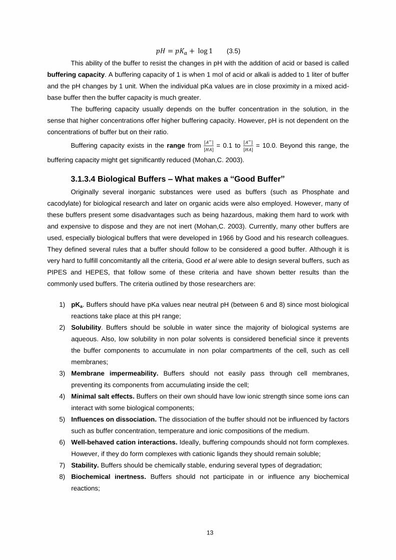
Buffer Buffer Range at 25ºC
Phosphate 7.2 - 7.4
PBS 7.2 - 7.6
Cacodylate 6.4 - 7.4
PHEM
Not known for buffer solution
PIPES - 6.1 - 7.5
HEPES - 6.8 - 8.2
EGTA - Neutral
Water Neutral
Table 3: Summary of buffer range at 25ºC of the different used buffers.
3.1.4 Effects of chemical fixation Samples fixed by different methods usually show some variation in ultrastructural details but
the overall structural relationship is maintained and subcellular organelles exhibit, in general, great
similarity. This means that whether samples were fixed with different chemicals as aldehydes (cross-
linkers), osmium tetroxide (oxidizer) or organic solvents (coagulators) or whether the sample was
vitrified, it shows the same characteristics, allowing it to be identified by an experienced observer.
These observations are evidence that the commonly seen relationships and structures are not an
artifact caused by a particular preparation method, but are a true representation of the in vivo
specimen (Crang, R., Klomparens, K., 1988).
However, it is helpful to know what are the main artifacts caused by each individual technique
since it is not always possible to do comparative studies for the same sample. A perfect fixation should
be artifact free (Crang, R., Klomparens, K., 1988). Therefore, knowing the artifacts produced by each
technique and how they arise can help us to optimize the fixation procedure so that artifacts do not
impair us to answer our biological question.
Discussed below are some of the most common artifacts caused by chemical fixation.
3.1.4.1 Changes in volume
During the processing of
samples for EM analysis the
specimens go through several
preparatory steps where changes
of volume can occur (Fig. 5). Also,
specimen weight can fluctuate
during these processes. It is
important to know how and when
these changes occur during
processing since they are an
indicator for the quality of
preservation of the fine structure.
In addition, inhibition of
cellular respiration will cause tissue
Fig. 5: Mean diameter of mouse ova during successive steps of preparation regarded as optimal (expressed as fraction of their
initial mean diameter in Brinster's medium – egg culture medium that contains mainly bovine serum albumin). The specimen showed the lowest volume in 100% ethanol and remained
unchanged after embedding in Epon (Konwinski et al., 1974).

18
swelling if the osmolarity is not maintained. When the tissue is fixed, cellular respiration stops
immediately and this can cause the tissue to swell. This swelling happens with an increase of water
flow towards the inside of the cell. This causes an uptake of ions that are dragged along with the
water. This is one of the reasons why during fixation slightly hypertonic solutions should be used.
Therefore, amount of shrinkage or swelling of the cell is a consequence of the osmolarity of
the fixative vehicle and the ion species that it contains, the concentration of the fixative and the
inherent characteristics of the tissue.
The fixation step is not the only step responsible for defining the final size of the specimen.
The conditions of dehydration and embedding can also influence the final size of the sample, as
shown in Fig. 5. This change in cell size is mainly a consequence of changes in the amount of water
inside the cell with changes in the size of subcellular components playing a minor role. However, it is
not clear that subcellular components undergo the same transitory changes in volume as the entire
cell. It is likely that the plasma membrane and the membranes of subcellular components have
different permeability values, and therefore it is expected that they respond differently to the same
osmotic gradient. Moreover, subcellular components encounter different osmotic gradients than the
plasma membrane (Eisenberg and Mobley, 1975). Therefore, the accurate volume of subcellular
components cannot be deduced from only measuring the cell. As an example, the cytoplasm and
nucleus can have different degrees of shrinkage. For instance, for the nucleus, fixation with
glutaraldehyde causes more shrinkage that fixation with osmium tetroxide or formaldehyde but the
contrary is true for the cytoplasm. Therefore, in the same cell, different size changes can be
happening at the same time for different subcellular components (Hayat, 1981).
As previously stated, aldehyde fixatives should be slightly hypertonic to help reducing cellular
artifacts. Hypotonic fixative solutions cause swelling of the tissue, while too hypertonic solutions cause
shrinkage. To avoid these artifacts, the solution would be to use an isotonic solution to fix the sample.
However, in practice isotonic fixative solutions have proven to be non satisfactory in preserving the
normal volume of intact tissues. Indeed, the total osmotic pressure that solute particles in a fixative
solution apply to a cell is not always related to its volume changes. The main reason for the failure of
isotonic fixative solutions in maintaining the cell volume has to do with the impossibility of measuring
the extracellular and intracellular osmolarity. Not having this information hinders the preparation of
isotonic fixative solutions. Also, different cell types have different intracellular osmotic pressure. In
addition, after removing a tissue from the body and depriving it from its in situ conditions may change
its cells osmolarity. And lastly, while fixing the tissue new ionized groups are formed.
Although fixation rapidly changes membrane permeability, there is maintenance of colloid-
osmotic equilibrium. Therefore, it is to this equilibrium that fixative osmolarity should be adjusted to
and not to the extracellular osmolarity, since they might differ.
Furthermore, when the samples are fixed with an isotonic fixative solution, the fixative
penetrates the membrane rather slowly. This is not desirable since the speed of membrane
penetration by the fixative influences the quality and rate of fixation. A slower penetration of fixative
may cause anoxia, since it takes longer to cease the cell metabolism, which in turn may cause
swelling (Hayat, 1981). Morphometric studies showed superior results in slightly hypertonic fixatives

19
since a constant surface-to-volume ratio is preserved by cell components under hypertonic conditions
of fixation (Hayat, 1981).
However, adverse effects may occur if a tissue is fixed with excessive hypertonic solution.
These include artifactual widening of extracellular spaces and separation of cytoplasm from the
nuclear membrane. Also, cell organelles that don’t have direct contact with the interstitial fluid, such as
mitochondria, shrink in volume proportionally to the decrease in cell volume in hypertonic solutions,
while organelles in direct contact with the interstitial fluid (e.g., transverse tubules) either swell or
remain unchanged.
It is clear that the changes in tissue volume that occur in the cell are caused by the artifacts
introduced during the many sample preparatory steps. However, in part, some of the final shrinkage or
swelling of the cell is directly connected to the ability of the primary fixative solution to maintain or not
its original volume. The reliability of the preparatory procedure and its capacity of producing quality of
specimen preservation can be assessed by the ability of maintaining the sample’s original in vivo size
(Hayat, 1981).
3.1.4.2 Reorganization in the plasma membrane
In vivo, there is equilibrium between the osmolarity in the extracellular and intracellular space
(isosmolarity). The membrane is permeable to small hydrophobic molecules and to small uncharged
polar molecules such as water. This means that water can enter or exit the cell simply through
diffusion or it can go through a special channel, called aquaporin. The latter is a passive process that
follows the direction of osmotic pressure across the membrane although many aquaporins function as
always-open channels. Conversely, large uncharged polar molecules and ions have to be actively
transported inside or outside the cell through the help of specialized channels or transporters (Cooper,
2000).
In the cytosol there are some macromolecules that, although few in number, are high in size
and highly charged, attracting many inorganic ions of opposite charge (counterions). Also, as a result
of active transport and metabolic processes there is a high concentration of small organic molecules,
such as amino-acids, which also attract counterions. There is also an abundance of inorganic ions
since they can only slowly leak across the plasma membrane to the cytosol. If they were not pumped-
out of the cell and if there were no interaction with other molecules inside the cell they would
eventually achieve an equilibrium state, where the extracellular concentration of ions would match the
intracellular concentration of ions. However, in the cytosol the macromolecules and small organic
molecules interact with the small inorganic ions and transporters pump them out of the cell. This
causes the environment in the interior of the cell to be electrically negative relative to its exterior, a
phenomena known as the Donnan effect. At the same time this difference in electric potential favors
the entry of positively charged ions into the cell such as Na+ (and the amino-acids “dragged” with it)
and opposes the entry of negatively charged ions, such as Cl-.
The most important transporter that helps the cell pump out the inorganic ions is the sodium-
potassium pump (Na+/K
+). It actively transports three Na
+ ions to the extracellular space while
importing two K+ ions concomitantly, by ATP hydrolysis (Lodish et al., 2000).
20
Since the Na+/K
+ pump drives different amounts of charged species in and out of the cell, it is
electrogenic. It drives a net current across the membrane, contributing to the maintenance of the
electrical potential of the cell, preserving the inside negative charge relative to the outside. Therefore,
energy is required to make these specific ion pumping systems work, maintaining a low concentration
of Na+
in the interior of the cell.
However, one of the major changes that happens after fixing a tissue is cellular membrane
reorganization which causes changes in membrane permeability and osmotic behavior. Different types
of cells may suffer different changes in their membranes after fixation but changes in osmotic
equilibrium happen to all plasma membranes (Cooper, 2000).
When the tissue is separated from the body and fixed, cellular respiration is inhibited and the
energy available for maintaining specific ion concentrations is diminished. With this, Na+ diffuses into
the cells without being actively extruded, and at the same time, K+
leaks out of the cells. This results in
Na+ accumulation inside the cells and loss of K
+, diminishing the negative potential of the plasma
membrane, allowing Cl- to enter the cells.
The net gain of solutes (especially osmotically active ones) by the cell causes a water flow
towards the inside of the cell and generates swelling of the tissue. This increased intracellular osmotic
pressure, if too extensive, may lead to autolysis of the cell (Hayat, 1981).
Although cellular membrane reorganization happens after fixation, it can happen in different
degrees. The most severe alteration happens with osmium tetroxide fixation. This fixative destroys the
differential permeability of the cellular membrane, allowing low-molecular-weight substances to pass
through it, including vital dyes. At the same time, this fixative decreases the fluidity of the membranes,
by perturbing lipid chains (Jost et al., 1973). Any damage caused to the cellular membrane will usually
lower its electrical resistance, and fixation with osmium tetroxide is not an exception.
On the other hand, a milder alteration happens to the cellular membrane when fixed with
glutaraldehyde, since it does not impair the relative impermeability of cellular membranes to the
majority of the ions. It is believed that after fixation with glutaraldehyde some reactive groups persist in
the membrane, and there is some evidence that suggest that glutaraldehyde-fixed cells remain
osmotically active (Fahimi and Drochmans, 1965).
According to Jard et al. (1966) and others, not only glutaraldehyde but also formaldehyde fixed
cells remain partly impermeable to ions (such as Na+). This is the reason that the osmolarity of
solutions used after fixation with glutaraldehyde may affect the cell structure.
The above stated superiority of glutaraldehyde over osmium tetroxide in terms of preserving
membrane osmotic selectivity does not seem to arise from the difference in penetration rates between
the two fixatives. It is likely that osmium tetroxide destabilizes the cell membrane by denaturing its
surface proteins. Another possibility suggested by Robertson (1959) is that this fixative is only able to
stabilize the inner most layer of the cell membrane while the most external layer breaks down into
chains of vesicles. Another factor that may contribute to the alteration of membranes is the action of
osmotic forces that can expand or contract the cytoplasm in a way that can cause the disruption and
recombination of the membranes (Doggenweiler and Heuser, 1967).

21
Additionally, it is assumed that reactive groups of adjacent cellular membranes interact, which
can lead to membrane reorganization if catalyzed by a substance used in subsequent steps of the
sample processing (e.g. organic solvents or unpolymerized embedding media) or by an increase in
temperature.
Finally, fixation with different reagents results in different alterations in cell membrane but also
fixation with a specific reagent can result in different alterations in different membrane (Hayat, 1981,
Daughty, 2004). It is obvious that the phenomenon of structural reorganization of membranes is still
not fully understood nor are all the factors that influence it.
3.1.4.3 Microtubules preservation
In vivo, microtubules are unstable structures and their preservation can be affected by several
factors. Low temperatures (around 4ºC), trauma during tissue preparation, autolysis, certain types of
fixatives and buffers, non-optimal osmolarity in fixative solutions, and excessive divalent cations
(especially Ca2+
) are some of the factors that can induce microtubule disassembly (Freeman, 2000).
There are various classes of microtubules and each one of them reacts differently to
temperature and fixation processes. Axonemal microtubules are usually considered to be more stable,
whereas cytoplasmatic microtubules are more unstable. Even microtubules of the same type can
present different stability. When microtubules are fixed with osmium tetroxide without a prefixation with
glutaraldehyde it is believed that they are no longer recognizable in most tissues. This happens since
the commonly used 1-2% aqueous solutions of osmium tetroxide at low temperature penetrate the
tissue too slowly to preserve microtubules. Therefore, it can be concluded that the fixative penetration
rate into the tissue and the interaction between fixative and sample are both important factor for
microtubule preservation. Taking this into consideration, for routine preservation of microtubules a
prefixation with glutaraldehyde at room temperature seems to be the most advisable choice.
Furthermore, if a secondary fixation with osmium tetroxide is used, then between the primary and
secondary fixation the temperature should be gradually decreased to 4ºC, to allow the specimen to
gradually acclimatize (Hayat, 1981).
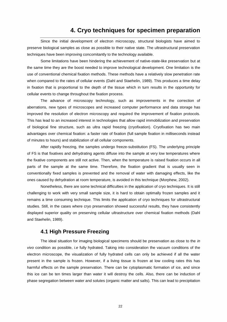
22
4. Cryo techniques for specimen preparation
Since the initial development of electron microscopy, structural biologists have aimed to
preserve biological samples as close as possible to their native state. The ultrastructural preservation
techniques have been improving concomitantly to the technology available.
Some limitations have been hindering the achievement of native-state-like preservation but at
the same time they are the boost needed to improve technological development. One limitation is the
use of conventional chemical fixation methods. These methods have a relatively slow penetration rate
when compared to the rates of cellular events (Dahl and Staehelin, 1989). This produces a time delay
in fixation that is proportional to the depth of the tissue which in turn results in the opportunity for
cellular events to change throughout the fixation process.
The advance of microscopy technology, such as improvements in the correction of
aberrations, new types of microscopes and increased computer performance and data storage has
improved the resolution of electron microscopy and required the improvement of fixation protocols.
This has lead to an increased interest in technologies that allow rapid immobilization and preservation
of biological fine structure, such as ultra rapid freezing (cryofixation). Cryofixation has two main
advantages over chemical fixation: a faster rate of fixation (full sample fixation in milliseconds instead
of minutes to hours) and stabilization of all cellular components.
After rapidly freezing, the samples undergo freeze-substitution (FS). The underlying principle
of FS is that fixatives and dehydrating agents diffuse into the sample at very low temperatures where
the fixative components are still not active. Then, when the temperature is raised fixation occurs in all
parts of the sample at the same time. Therefore, the fixation gradient that is usually seen in
conventionally fixed samples is prevented and the removal of water with damaging effects, like the
ones caused by dehydration at room temperature, is avoided in this technique (Morphew, 2002).
Nonetheless, there are some technical difficulties in the application of cryo techniques. It is still
challenging to work with very small sample size, it is hard to obtain optimally frozen samples and it
remains a time consuming technique. This limits the application of cryo techniques for ultrastructural
studies. Still, in the cases where cryo preservation showed successful results, they have consistently
displayed superior quality on preserving cellular ultrastructure over chemical fixation methods (Dahl
and Staehelin, 1989).
4.1 High Pressure Freezing
The ideal situation for imaging biological specimens should be preservation as close to the in
vivo condition as possible, i.e fully hydrated. Taking into consideration the vacuum conditions of the
electron microscope, the visualization of fully hydrated cells can only be achieved if all the water
present in the sample is frozen. However, if a living tissue is frozen at low cooling rates this has
harmful effects on the sample preservation. There can be cytoplasmatic formation of ice, and since
this ice can be ten times larger than water it will destroy the cells. Also, there can be induction of
phase segregation between water and solutes (organic matter and salts). This can lead to precipitation

23
of cellular components between ice crystals which can be visible in electron micrographs (Dubochet
2007).
Ice formation in the cell can be deleterious since ice crystals can grow and create holes in the
cellular membranes leading to the destruction of organelles. When these badly frozen samples are
thawed again they are already completely destroyed. This harmful ice crystal formation can be
avoided if the biological samples are protected with anti-freeze agents that reduce the concentration of
free water (Dubochet 2007).
When freezing a biological sample, the freezing rate should be fast enough so that the ice
crystals formed are smaller than the resolution of the electron microscope (smaller than 10-15nm) or
that vitreous ice is formed. The method to obtain these conditions is called ultrarapid freezing. The
most commonly used methods of cryo immobilization are: 1) plunge freezing, 2) propane jet freezing,
3) cold metal block freezing and 4) high-pressure freezing. However, for the first three methods
successful preservation is only achieved on very thin samples, such as a monolayer of cells. Only the
fourth one, high pressure freezing, allows successful preservation of samples up to theoretically
600µm of thickness.
To achieve acceptable freeze-fixation, freezing rates of more than - 10,000ºC/sec are required
for most biological specimens. However, for samples thicker than 20 µm this rate cannot be achieved
in the middle of the sample due to the low heat conductivity of water. Because of this, some types of
samples cannot be preserved by ultrarapid freezing methods at atmospheric pressure.
For successful preservation on thicker samples, the physical properties of the water need to
be changed by reducing the critical rate of freezing in order to create a small size ice crystal (Moor,
1987). One way of achieving this is with the application of cryoprotectants. Although the use of
cryoprotectants helps to reduce water’s freezing rate to between -100 and -500ºC/sec it is not always
innocuous. The addition of natural cryoprotectants in most cases is not possible and therefore the use
of artificial cryoprotectants is adopted. However, high concentration (20-30%) of these artificial
cryoprotectants and their dehydrating activity can lead to changes in cell morphology (such as severe
shrinking and specific responses to osmotic stress) which essentially removes the advantages of cryo
fixation. To overcome this problem, freezing under high pressure should be adopted for preserving
samples thicker than 20µm. As discussed in several papers (Meryman, 2007; Dahl and Staehelin,
1989) the reduction of the freezing rate by high pressure freezing is achieved by some changes in the
freezing properties of water, namely:
1) Decreasing the freezing point of water;
2) Reducing the nucleation rate of ice crystals;
3) Diminishing the growth of ice crystals.
4.2 Physics of ice formation in biological specimens
There are three forms of pure water in the solid state. Two of them are crystalline forms,
hexagonal crystal and cubic crystal. The third, also called vitreous form, happens when water is frozen
so rapidly that crystals don’t have enough time to be formed and water remains amorphous. Since
crystal formation causes water expansion as it freezes and vitreous ice is the same size as liquid
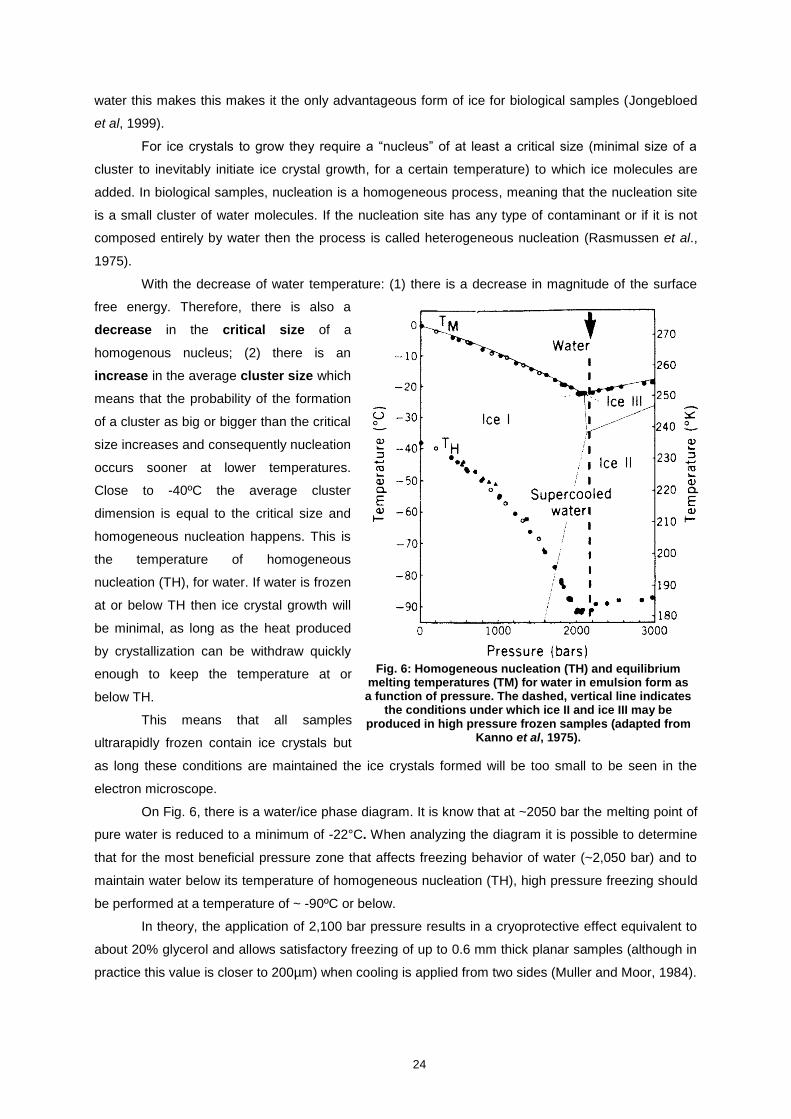
24
water this makes this makes it the only advantageous form of ice for biological samples (Jongebloed
et al, 1999).
For ice crystals to grow they require a “nucleus” of at least a critical size (minimal size of a
cluster to inevitably initiate ice crystal growth, for a certain temperature) to which ice molecules are
added. In biological samples, nucleation is a homogeneous process, meaning that the nucleation site
is a small cluster of water molecules. If the nucleation site has any type of contaminant or if it is not
composed entirely by water then the process is called heterogeneous nucleation (Rasmussen et al.,
1975).
With the decrease of water temperature: (1) there is a decrease in magnitude of the surface
free energy. Therefore, there is also a
decrease in the critical size of a
homogenous nucleus; (2) there is an
increase in the average cluster size which
means that the probability of the formation
of a cluster as big or bigger than the critical
size increases and consequently nucleation
occurs sooner at lower temperatures.
Close to -40ºC the average cluster
dimension is equal to the critical size and
homogeneous nucleation happens. This is
the temperature of homogeneous
nucleation (TH), for water. If water is frozen
at or below TH then ice crystal growth will
be minimal, as long as the heat produced
by crystallization can be withdraw quickly
enough to keep the temperature at or
below TH.
This means that all samples
ultrarapidly frozen contain ice crystals but
as long these conditions are maintained the ice crystals formed will be too small to be seen in the
electron microscope.
On Fig. 6, there is a water/ice phase diagram. It is know that at ~2050 bar the melting point of
pure water is reduced to a minimum of -22°C. When analyzing the diagram it is possible to determine
that for the most beneficial pressure zone that affects freezing behavior of water (~2,050 bar) and to
maintain water below its temperature of homogeneous nucleation (TH), high pressure freezing should
be performed at a temperature of ~ -90ºC or below.
In theory, the application of 2,100 bar pressure results in a cryoprotective effect equivalent to
about 20% glycerol and allows satisfactory freezing of up to 0.6 mm thick planar samples (although in
practice this value is closer to 200µm) when cooling is applied from two sides (Muller and Moor, 1984).
Fig. 6: Homogeneous nucleation (TH) and equilibrium melting temperatures (TM) for water in emulsion form as a function of pressure. The dashed, vertical line indicates
the conditions under which ice II and ice III may be produced in high pressure frozen samples (adapted from
Kanno et al, 1975).

25
4.2.1 Technology of high pressure freezing To freeze a sample in the HPF machine, first the sample has to be introduced into a special
sample holder (carrier). There are different types of carriers depending on what type of sample is used
and also for different applications (Studer, 2008) and different machines.
First, the carrier should be selected to fit the sample size without damaging it and at the same
time preventing extra space (unnecessary volume creates heat that must be extracted). Also, there
should not be any space filled with air inside the carrier. Air bubbles within the carrier act as insulators
and collapse under pressure which can lead to sample damage (Dahl, Staehelin 1989). Therefore, all
enclosed air spaces should be filled with sample or fluid.
There are a wide variety of carriers. The ones used in this study were aluminum. They have
two hats. Generally one type is "welled" and the other smooth so they can be combined. If two welled
hats are used, a larger cavity is created while a combination of a welled and a flat hat decreases the
size of the cavity by half. This type of carriers can suffer damage during freeze substitution and
therefore are usually discarded after one usage (Studer, 2008).
To achieve the best freezing rate the type of holder and the medium that surrounds the
sample must be optimized. As previously said, the volume inside the carrier that is filled with air should
be replaced with a medium. The success of the freezing process relies upon the type of sample being
frozen since different samples possess different water content and even the same cell has different
water content between cytoplasm and organelles. Also, the freezing success can also vary due to
naturally cryoprotective action within a sample. For the majority of the samples, the best choice of
"filler" is one that possesses some cryoprotection capacity. Cryoprotectants suppress ice crystal
formation and expansion, which leads to reduced heat release in the crystallization process. This
improves the cooling rate of the sample, increasing the quality of freezing (Dahl, Staehelin, 1989).
There are a wide variety of cryoprotectants that can preserve the samples without having any
interaction with them, and without influencing any cellular process (Morphew, 2002). They can be
non-penetrative and hydrophobic substances that have low osmotic activity such as 1) serum
albumin (10-20%); 2) low melting agarose (0.5% - 2.0%); 3) dextran (15-20%); 4) cold water fish
gelatin (50-100%); 5) polyvinylpyrolidone (15%); 6) Ficol (5-15%); 7) 1-hexadecene; or they can be
penetrative on some tissues such as sucrose (150mM) or methanol (10%) in yeast paste for filler.
Since the goal of vitrifying a sample is to allow its
ultrastructural observation in a close to native state, it is
important to minimize as much as possible the time between
sample collection and freezing.
The Wohlwend HPF machine, developed according
to Moor et al. (1980), pressurizes liquid nitrogen to ~2050 bar
and then “shoots” it onto the sample holder to freeze the
specimen, making the cryogen to act as a pressurizing agent.
Pressurization and cooling of the sample are synchronized to
occur within 20 ms in both systems (Fig. 7). Fig. 7: Record of pressure (purple line) and temperature (yellow line) changes during freezing (total time = ~380 ms)
in the Wohlwend Compact 02 high pressure freezing machine.
Temperature drops approximately -120ºC.

26
4.3 Freeze substitution
With the pioneering work of Müller and Steinbrecht an old EM method called freeze
substitution regained importance since it has proven to the best routine method for processing high
pressure frozen samples. It allows relatively high quality structural preservation and also allows the
use of immunogold and fluorescent techniques by combining cryofixation with resin embedding.
In freeze substitution, fixatives are added to the sample at very low temperatures (around -
90ºC). They will diffuse into the cells at this temperature but not react (cross-linking) with cellular
components. The fixatives only start to act at higher temperatures (~-50ºC for glutaraldehyde and ~-
30ºC for osmium tetroxide) (Humbel and Müller 1986). Since chemical fixatives are already diffused
throughout the sample when the cross-linking temperature is achieve, there is no diffusion-related
fixation artifacts like the ones caused by conventional room-temperature methods and therefore no
osmotic effects occur (Studer et al. 1992).
For freeze substitution the fixatives (glutaraldehyde or osmium tetroxide) are diluted in an
organic solvent such as methanol or acetone. In the same cocktail uranyl acetate can be added to
help improve membrane contrast. Under these conditions formation of cubic ice crystals may occur
but typically their size is below the TEM resolution therefore the small crystals do not noticeably
damage cellular ultrastructure (Kent, 2013).
Since the fixatives are diluted in organic solvent this means that dehydration of the samples
starts at the same times as fixation. At these low temperatures, large molecules (such as proteins) are
immobilized but smaller molecules (such as water) can be dissolved and replaced with the organic
solvent.
After the freeze substitution is complete the samples can be brought up to room temperature
without the risk of recrystallization since water is now absent from the sample.
The main advantages of this freeze substitution are:
1) Fixatives are already diffused through the sample prior to warming, which is when their
cross-linking activity begins.
2) Dehydration takes place at very low temperatures, which helps to prevent ultrastructural
artifacts as caused by room temperature dehydrations.
3) Samples can be processed for immunochemistry techniques. Since the sample is infiltrated
and resin polymerized at low temperature, epitopes are more protected from damaging
effects (Morphew, 2002).
27
5. Cilia
Cilia are 9-fold symmetric microtubule-based structures that protrude from the cell membrane.
They can be motile or immotile and they have several functions in the cells such as promoting motility
(in the sperm flagellum), stirring particles around (in the respiratory epithelium) and responding to
various external signals (intercellular communication). As shown in Fig. 8, the cilium has two
compartments: (1) the transition zone which is linked to a basal body docked to the cell membrane
and (2) the axoneme (Jana et al, 2014).
At the transition zone the doublet microtubules are heavily cross-linked to the surrounding
ciliary membrane by structures called y-linkers. The transition zone may act as a gatekeeper for
material that goes into the cilia. The doublet MTs of the transition zone are thought to be a template
for the MT skeleton of the cilium, also called axoneme, which consequently exhibits a 9-fold symmetry
(Carvalho-Santos, 2012).
Since cilia are a component of most eukaryotic cells, when these organelles are altered they
can lead to a wide variety of human diseases, which are referred to as ciliopathies. These diseases
present a large spectrum of conditions including various syndromes, sterility, microcephaly, situs
inversus, polycystic kidney disease, retinal degeneration, and dwarfism (Waters, A. Beales, P., 2011).
Also, alterations of these organelles have been linked to cancer. All of these implications caused by
cilia alterations stress the need of having a better understanding of cilia biology and structure.
The structures described above were initially studied using conventional TEM, revealing
remarkable features and structural complexity (Jana et al, 2014). Much more can be studied and
learned using both the conventional electron microscopy approach and cryo techniques for tissue
fixation. Also employing other modern techniques such as super-resolution light microscopy, x-ray
crystallography, and cryoelectron tomography can gives us new insights (Carvalho-Santos, 2012).
To carry out these techniques, model organisms need to be used. Since cilia are conserved
eukaryotic organelles several different model can be used such as Drosophila melanogaster (Dm)
(Jana et al, 2014).
Fig. 8: Schematic representation of a longitudinal view of the cilium and its compartments. (Jana et al, 2014).

28
5.1 Drosophila melanogaster
Dm is a model organism widely used to research the fundamental mechanism of biological
processes. For many reasons it is an excellent model to study the biology of centrosomes and cilia by
fluorescent microscopy and also electron microscopy (Jana et al, 2014). Some of these reasons
include the following: Many diverse cilia found in several uni and multi-cellular organisms are present
within this single organism, the fruit fly (Briggs et al, 2014). Secondly, several genetic tools are already
available and fly mutants of ciliary proteins are not embryonic lethal (Basto el al, 2006). Moreover,
fertility, sensory responses and behavioral assays can serve as an output for fly ciliary functions
(Enjolras, 2012). Also, nearly 75% of human disease-causing genes are believed to have a functional
homolog in the fly. Lastly, short generation time, very low comparative costs and minimal ethical
problems make Dm a unique organism to study cilia (Pandey, U. Nichols, C., 2011)
A pair of antennae is located on the front of the head of Dm, between the eyes. Each antenna
serves as a sound and mechanical stimuli transducer, creating an electrochemical answer in the
peripheral nervous system (Todi, 2004). Olfactory and auditory stimuli are detected by ciliated sensory
neurons, on the third and second segment of the antenna respectively. At the distal tip of those
neurons there is a cilium, serving as a bridge between the received stimuli and the cell body of the
neuron (Vincensini, 2011).
The antenna is caped with an exoskeleton, the cuticle. This structure contains lipids and
polysaccharide chitin, serving as a protective barrier and as an interface with the environment
(Boseman et al, 2013). However, since chitin is a tough material it is hard to process for electron
microscopy.
Each antenna consists of three segments (first segment – scape, second segment – pedicel
and third segment – funiculus) and a thin arista (Fig. 9). The arista is the main sensory organ that
receives sound. When there is a stimulus, the arista vibrates and activates the third segment of the
antenna that twists relatively to the second segment. A thin stalk connects both segments and
encloses the antennal nerve that descends until the third segment. The signal goes until the second
segment, to the Johnston’s organ where the chordotonal sensory neurons are. The axons of the
Fig. 9: Schematic representation of the head of Drosophila melanogaster. The inset shows one of the two antennae that are positioned between the eyes of the fly. In the inset the several segments of the antenna
are represented as well as the arista, another sensory organ.
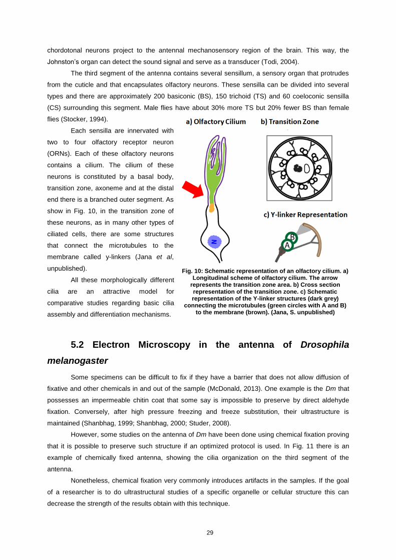
29
chordotonal neurons project to the antennal mechanosensory region of the brain. This way, the
Johnston’s organ can detect the sound signal and serve as a transducer (Todi, 2004).
The third segment of the antenna contains several sensillum, a sensory organ that protrudes
from the cuticle and that encapsulates olfactory neurons. These sensilla can be divided into several
types and there are approximately 200 basiconic (BS), 150 trichoid (TS) and 60 coeloconic sensilla
(CS) surrounding this segment. Male flies have about 30% more TS but 20% fewer BS than female
flies (Stocker, 1994).
Each sensilla are innervated with
two to four olfactory receptor neuron
(ORNs). Each of these olfactory neurons
contains a cilium. The cilium of these
neurons is constituted by a basal body,
transition zone, axoneme and at the distal
end there is a branched outer segment. As
show in Fig. 10, in the transition zone of
these neurons, as in many other types of
ciliated cells, there are some structures
that connect the microtubules to the
membrane called y-linkers (Jana et al,
unpublished).
All these morphologically different
cilia are an attractive model for
comparative studies regarding basic cilia
assembly and differentiation mechanisms.
5.2 Electron Microscopy in the antenna of Drosophila
melanogaster
Some specimens can be difficult to fix if they have a barrier that does not allow diffusion of
fixative and other chemicals in and out of the sample (McDonald, 2013). One example is the Dm that
possesses an impermeable chitin coat that some say is impossible to preserve by direct aldehyde
fixation. Conversely, after high pressure freezing and freeze substitution, their ultrastructure is
maintained (Shanbhag, 1999; Shanbhag, 2000; Studer, 2008).
However, some studies on the antenna of Dm have been done using chemical fixation proving
that it is possible to preserve such structure if an optimized protocol is used. In Fig. 11 there is an
example of chemically fixed antenna, showing the cilia organization on the third segment of the
antenna.
Nonetheless, chemical fixation very commonly introduces artifacts in the samples. If the goal
of a researcher is to do ultrastructural studies of a specific organelle or cellular structure this can
decrease the strength of the results obtain with this technique.
Fig. 10: Schematic representation of an olfactory cilium. a) Longitudinal scheme of olfactory cilium. The arrow
represents the transition zone area. b) Cross section representation of the transition zone. c) Schematic representation of the Y-linker structures (dark grey)
connecting the microtubules (green circles with A and B) to the membrane (brown). (Jana, S. unpublished)

30
To overcome this problem, and to achieve a
greater level of precision, cryo fixation techniques can be
used. This method usually produces improved structural as
preservation when compared to chemical fixation methods
(Fig. 12) (McDonald, 2013).
Several cryo-fixation techniques were adapted for
Dm tissues. However, so far there are no reports in the
literature of a cryo-fixation study that focuses on the
antenna of the Dm, in particular the third segment.
One of the challenges with this tissue is that it has a
wide amount of empty space to allow neurons to vibrate.
Air, however affects the success of high pressure freezing
since while applying high pressures to a tissue, if it contains
air it can collapse (McDonald, 2007).
One way to overcome this problem can be trying to
fill these empty spaces before high pressure freezing the
sample. It is described that the quality of samples fixed with
aldehydes prior to being high pressure frozen is very similar
to the ones high pressure frozen without the fixation step
and superior to conventional glutaraldehyde fixation
methods (Sosinsky et al., 2008). Therefore, one solution could be to put the sample in fixative prior to
high pressure freezing and allow the fixative to penetrate the sample, fixing it and filling the empty
spaces.
Fig. 12: Low-magnification views of epidermal cells processed by HPF-FS (A) or conventional fixation
(B). Scale bars, 1 μm (McDonald, 2014).
Fig. 11: Anatomy of olfactory cilium (Jana, 2011).

31
6. Methodology
In this study, relationships between phenomena are going to be analyzed. Therefore,
accordingly to Fortin this study can be classified as a correlational study (Fortin, 2000). As for the
manipulation of variables, this is an experimental study, because the independent variables are going
to be manipulated and an alteration of the dependent variables is expected. This is also a quantitative
study, because the methodology is going to be based on a systematic process of data analysis
quantifying objective outputs that occur independently of the researchers (Fortin, 2000).
6.2 Sampling and sample
Sampling was non probabilistic because there is a deliberate choice of the sample elements,
and it is not representative of the entire population. It is accidental, since the organ was chosen by
convenience, not being possible to generalize the results to other organs.
For chemical fixation the sample consists of 40 antennas. The samples were divided as
outlined in Table 4 (times 2 rounds of processing):
Table 4: Sample division for chemical processing according to each analyzed buffer.
For the freeze substitution protocol the samples were divided as shown in Table 5. There are
48 antennas (4 antennas x 4 carriers per condition x 2 rounds of processing per condition):
2% Formaldehyde and 2,5% Glutaraldehyde
Phosphate
4 heads
8 third segments (pierced)
PHEM
4 heads
8 third segments (pierced)
Cacodylate
4 heads
8 third segments (pierced)
PBS
4 heads
8 third segments (pierced)
Water
4 heads
8 third segments (pierced)
1% OSO4, 0,5% Uranyl acetate and 5% water in Acetone
Fast FS
6hrs30min
32 antennas
Medium FS
19hrs30min
32 antennas
Long FS
52hrs
32 antennas
Table 5: Sample division for cryo processing according to each parameter to analyze.

32
6.3 Lab work
All the lab work was done at the Instituto Gulbenkian de Ciência in the Cell Cycle Regulation
Laboratory and in the Electron Microscopy Facility.
6.4 Methods for chemical fixation
6.4.1 Sample processing solutions
6.4.1.1 Sodium bi-Phosphate buffer
Stock solution A and B was first made:
o Stock solution A: 0.2M monobasic sodium phosphate, monohydrate (27.6 g NaH2PO4
was dissolved in 1 L Milli-Q water).
o Stock solution B: 0.2M dibasic sodium Phosphate (28.4 g Na2HPO4 was dissolved in
1 L Milli-Q water).
28mL of stock solution A was mixed with 72mL of stock solution B to obtain 100mL of 0.2M of
Phosphate buffer pH 7.2.
6.4.1.2 PBS buffer
Phosphate buffered saline tablets were used.
o 1 tablet of PBS was diluted in 150mL of WFI quality water to obtain 150mL of 0.2M
PBS buffer.
6. 4.1.3 Cacodylate buffer
375mL of WFI quality water were measured.
21.4g of sodium Cacodylate (Na(CH3)2 AsO2 • 3H2O) were added to the water.
The solution was mixed and the pH adjusted to 7.4
When the pH was stabilized more water was added to the solution until made up to obtain
500mL of 0.2M Cacodylate buffer.
6. 4.1.4 PHEM buffer
4 NaOH pellets (approximately 1g) were diluted in 75mL of WFI quality water.
3.63g of PIPES (120mM) were added to the solution.
The pH was set to 7.0. After the solution turned clear the following steps were performed:
To the solution the following was added: 1.3g of HEPES (for a final concentration of 50mM),
0.08g of MgCl2.6H20 (final concentration 4mM), 0.76g of EDTA (final concentration 20mM).
The pH was adjusted to 7.4.
The volume was made up to 100mL with WFI quality water to obtain a final solution of 100mL
of 0.2M PHEM buffer.

33
6. 4.1.5 Fixative for chemical Fixation
To make 100mL of fixative solution (2% Formaldehyde, 2,5% Glutaraldehyde in 0.1M buffer),
12.5mL of 16% formaldehyde (EM grade), 10mL of 25% glutaraldehyde (EM grade), 27.5mL WFI
quality water and 50mL of 0.2M buffer (one of each of the previously mentioned) were mixed.
6.4.1.6 Uranyl Acetate solution
2% UA in d-water (20 g/L) and 2% UA in 70% methanol (20 g/L) were used for sample
fixation/processing and for the staining of ultra-thin sections, respectively.
6.4.1.7 Reynold’s Lead Citrate
30mL de-carbonated water was made by boiling the d-water in a microwave and by cooling
the water in a freshly washed sealed container. 30mL of de-carbonated water was added to 1.33g of
lead nitrate and 1.76g of sodium citrate into a volumetric flask and shaken vigorously for 1min followed
by sonication for 30min. The container was agitated at five minutes intervals. 8.0mL of 1N sodium
hydroxide (NaOH) was added in the opaque mixture and the mixture would then turn clear. The
volume was brought up to 50mL with the de-carbonated water. The solution was stored in a tightly
sealed volumetric flask. NOTE: The solution should be stored in a sealed container, since lead citrate
reacts with carbon dioxide (CO2) to form lead carbonate precipitate.
6.4.1.8 EPONTM Epoxy resin
Stock solutions were first made:
o Stock EPON I: 62mL of EMbed 812 and 100mL of dodecenyl succinic anhydride
(DDSA) were mixed.
o Stock EPON II: 100mL of EMbed 812 and 90mL of nadic methyl anhydride (NMA)
EPON working solution were mixed according to Luft (1961).
NOTE: These two stock solutions should be stored at 4ºC separately. Since both EPON I and
EPON II are strongly hydroscopic, the stock solutions should be mixed just before the mixture
is used and warmed up before the containers are opened.
To make the working EPON solution, 30mL of EPON I was then mixed with 70mL of EPON II
and 1.5mL of Tris-(dimethylaminomethyl) phenol (DMP-30) (accelerator) was added.
6.4.2 Chemical Fixation Protocol
1) Flies were put to sleep with CO2 and the heads were removed from the fly.
2) The heads were immersed in fixative (2% formaldehyde, 2.5% glutaraldehyde in 0.1M buffer
(either Phosphate, PHEM, cacodylate, PBS or simply WFI quality water) pH 7.4) for 30min.
3) The third antennal segments were pierced using a thin tungsten needle.
4) Heads were transferred to the same fixative and were fixed overnight at 4ºC with rotation.
5) The samples were washed for 5 x 5min in the buffer used for the fixative solution.
6) The samples were post-fixed in 1% osmium tetroxide (OsO4), for 1hr30min at 4ºC.
7) The samples were washed with Milli-Q water for 5 x 5min
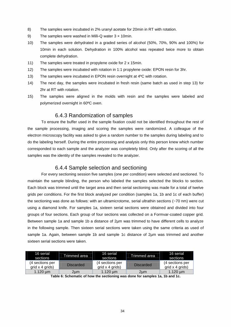
34
8) The samples were incubated in 2% uranyl acetate for 20min in RT with rotation.
9) The samples were washed in Milli-Q water 3 × 10min.
10) The samples were dehydrated in a graded series of alcohol (50%, 70%, 90% and 100%) for
10min in each solution. Dehydration in 100% alcohol was repeated twice more to obtain
complete dehydration.
11) The samples were treated in propylene oxide for 2 x 15min.
12) The samples were incubated with rotation in 1:1 propylene oxide: EPON resin for 3hr.
13) The samples were incubated in EPON resin overnight at 4ºC with rotation.
14) The next day, the samples were incubated in fresh resin (same batch as used in step 13) for
2hr at RT with rotation.
15) The samples were aligned in the molds with resin and the samples were labeled and
polymerized overnight in 60ºC oven.
6.4.3 Randomization of samples To ensure the buffer used in the sample fixation could not be identified throughout the rest of
the sample processing, imaging and scoring the samples were randomized. A colleague of the
electron microscopy facility was asked to give a random number to the samples during labeling and to
do the labeling herself. During the entire processing and analysis only this person knew which number
corresponded to each sample and the analyzer was completely blind. Only after the scoring of all the
samples was the identity of the samples revealed to the analyzer.
6.4.4 Sample selection and sectioning For every sectioning session five samples (one per condition) were selected and sectioned. To
maintain the sample blinding, the person who labeled the samples selected the blocks to section.
Each block was trimmed until the target area and then serial sectioning was made for a total of twelve
grids per conditions. For the first block analyzed per condition (samples 1a, 1b and 1c of each buffer)
the sectioning was done as follows: with an ultramicrotome, serial ultrathin sections (~70 nm) were cut
using a diamond knife. For samples 1a, sixteen serial sections were obtained and divided into four
groups of four sections. Each group of four sections was collected on a Formvar-coated copper grid.
Between sample 1a and sample 1b a distance of 2µm was trimmed to have different cells to analyze
in the following sample. Then sixteen serial sections were taken using the same criteria as used of
sample 1a. Again, between sample 1b and sample 1c distance of 2µm was trimmed and another
sixteen serial sections were taken.
16 serial sections
Trimmed area 16 serial sections
Trimmed area 16 serial sections
(4 sections per grid x 4 grids)
Discarded (4 sections per grid x 4 grids)
Discarded (4 sections per grid x 4 grids)
1.120 µm 2µm 1.120 µm 2µm 1.120 µm Table 6: Schematic of how the sectioning was done for samples 1a, 1b and 1c.
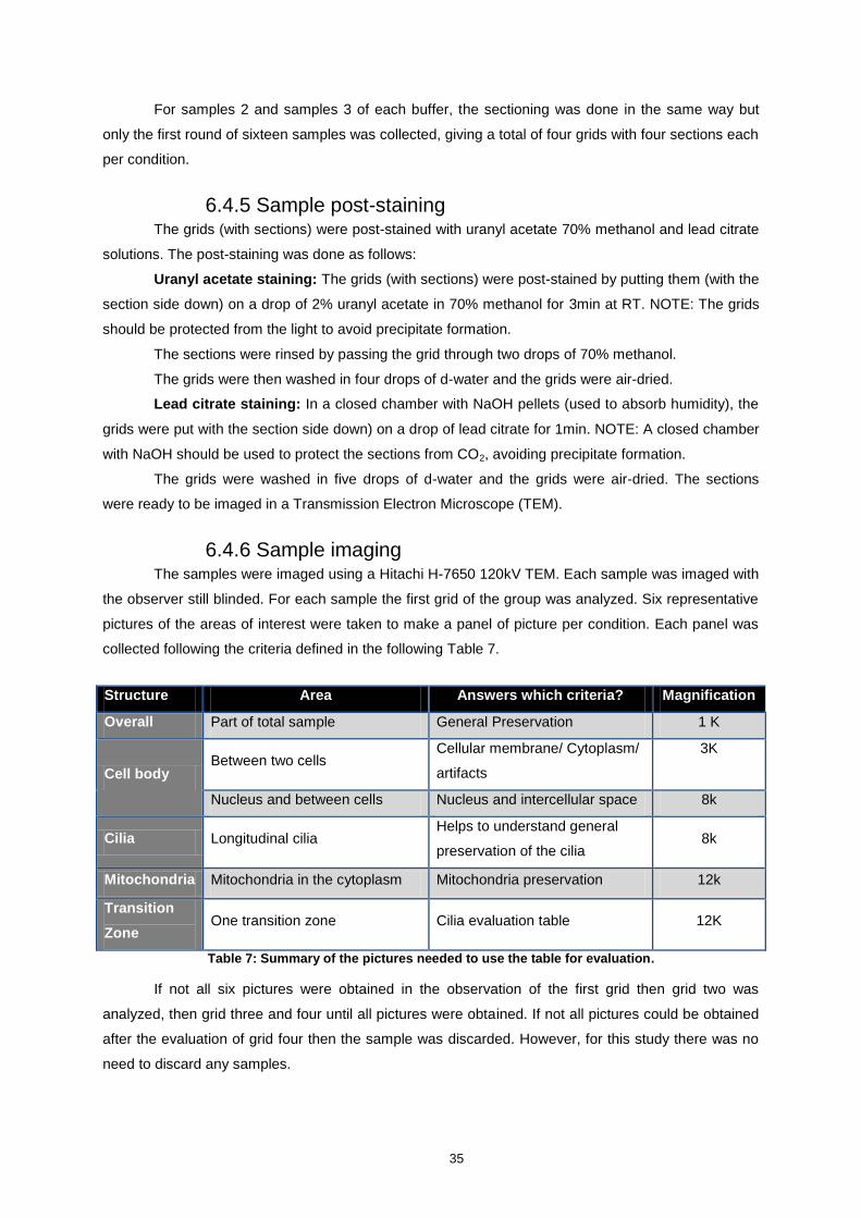
35
For samples 2 and samples 3 of each buffer, the sectioning was done in the same way but
only the first round of sixteen samples was collected, giving a total of four grids with four sections each
per condition.
6.4.5 Sample post-staining The grids (with sections) were post-stained with uranyl acetate 70% methanol and lead citrate
solutions. The post-staining was done as follows:
Uranyl acetate staining: The grids (with sections) were post-stained by putting them (with the
section side down) on a drop of 2% uranyl acetate in 70% methanol for 3min at RT. NOTE: The grids
should be protected from the light to avoid precipitate formation.
The sections were rinsed by passing the grid through two drops of 70% methanol.
The grids were then washed in four drops of d-water and the grids were air-dried.
Lead citrate staining: In a closed chamber with NaOH pellets (used to absorb humidity), the
grids were put with the section side down) on a drop of lead citrate for 1min. NOTE: A closed chamber
with NaOH should be used to protect the sections from CO2, avoiding precipitate formation.
The grids were washed in five drops of d-water and the grids were air-dried. The sections
were ready to be imaged in a Transmission Electron Microscope (TEM).
6.4.6 Sample imaging The samples were imaged using a Hitachi H-7650 120kV TEM. Each sample was imaged with
the observer still blinded. For each sample the first grid of the group was analyzed. Six representative
pictures of the areas of interest were taken to make a panel of picture per condition. Each panel was
collected following the criteria defined in the following Table 7.
Structure Area Answers which criteria? Magnification
Overall Part of total sample General Preservation 1 K
Cell body Between two cells
Cellular membrane/ Cytoplasm/
artifacts
3K
Nucleus and between cells Nucleus and intercellular space 8k
Cilia Longitudinal cilia Helps to understand general
preservation of the cilia 8k
Mitochondria Mitochondria in the cytoplasm Mitochondria preservation 12k
Transition
Zone One transition zone Cilia evaluation table 12K
Table 7: Summary of the pictures needed to use the table for evaluation.
If not all six pictures were obtained in the observation of the first grid then grid two was
analyzed, then grid three and four until all pictures were obtained. If not all pictures could be obtained
after the evaluation of grid four then the sample was discarded. However, for this study there was no
need to discard any samples.

36
6.4.7 Sample evaluation
6.4.7.1 Variables
In accordance with the objectives outlined, the following are considered dependent and
independent variables for each type of processing (chemical and cryo processing):
Independent variables: In this study, the independent variable for the chemical processing
protocol is the type of buffer (Phosphate, PHEM, cacodylate, PBS or water. For the cryo processing
protocol the independent variable is the duration of FS protocol (rapid- 6hr30min, medium –
19hr30min or slow – 52hr).
Dependent variables: The dependent variables, conditioned by manipulating the previously
mentioned independent variables, are considered to be the final quality of samples observed by TEM,
which is based on ten parameters:
General preservation – any electron microscopy technique should maintain the cell
structures in a close to native state of preservation, to allow proper observation of areas of
interest and to ensure a reliable characterization of the entire sample;
Cellular membrane preservation – the membrane should be continuous, have a smooth
contour along the entire cell and there should not be any vesiculation (blebbing) present;
Cytoplasm preservation – the cytoplasmic content should be evenly distributed throughout
and not show areas of clumping or empty spaces;
Intercellular space preservation – the space between cells should be narrow and empty
space should not be visible. The intercellular space was measured in several HPF
pictures (Sanbhag, S. et al. 1999, 2000) to determine a mean value that resembles a
close to native state;
Nuclear preservation – Nucleus should maintain the expected shape for the type of cell
and cell cycle; the double membrane should be visible and evenly spaced through the
entire nuclear contour; the contour should be smooth around the entire nucleus;
Mitochondria preservation - Mitochondria should have the expected shape and the
membrane should be visible and not ruffled;
Artifacts – there should be no artifacts resulting from the fixation method - neither
extraction in the chemical fixation protocol nor ice crystal in the cryo fixation protocol;
Ciliary membrane preservation – the ciliary membrane should be continuous and round
shaped;
Microtubule preservation – On a clear cross-section of the transition zone, the doublet
microtubules should be visible;
Preservation of other structures - On a clear cross-section of the transition zone, the y-
linker structures should be visible and the electron density surrounding the microtubules
should not impair their visualization.
To analyze these dependent variables and be able to understand the influence of the
independent variables in the ultrastructural preservation of the sample a table with a set of criteria
were defined. The criteria defined are based on the dependent variables that were to be evaluated.

37
The table was constructed specifically to allow the comparison between each protocol (either
the chemical fixation protocol or the cryo fixation protocol). The table is divided into two main topics:
general preservation of the sample and the cilia preservation in the tissue. Together, these two topics
make the Criteria table for judging ultrastructural preservation. The example of the table created to
evaluate each protocol is presented below (Tables 8 and 9).
To ensure an unambiguous interpretation, each parameter was defined by assigning it a value
for both Table 8 and Table 9 (an evaluation of “no” corresponds to a 0 and an evaluation of “yes”
corresponds to a 1). For each value a specific description was created that clarifies the criteria to be
used by the observer, with the aim of standardizing the evaluation process across different samples
and different observers. The maximum total that can be obtained with this quantitative analysis for the
final evaluation score (general score + cilia score) is a total score of 20 (all parameters with positive
evaluation) and the minimum total that can be achieved is a total of 1 (all parameters with negative
evaluation except parameter G15). The minimum value that can be achieved for the final evaluation
cannot be 0 since giving a negative evaluation to parameter G15 in the general evaluation table
automatically invalidates the evaluation of the sample.
The observer was only allowed to know the identity of each sample after all the evaluation
tables were filled, so that the final results could be analyzed.
After the observer analyzed all the samples, four of them were selected. These samples are
representative of different difficulties to analyze. It was chosen one easy, two medium and one hard
sample to analyze, corresponding to samples A- Water (sample 3), B- Phosphate (sample 1b), C-
Water (sample 1a) and D- PBS (sample 3). These four samples were coded with the letter just
mentioned (A, B, C and D) and given to three other observers, with different backgrounds and EM
experience, to judge if the table can be used by different EM experienced users. The observers
selected were one EM technician, one biologist and one air traffic controller. The identity of all the
samples remained unknown to all the observers until the end of the evaluation.

38
General Evaluation Table
Structure Criteria Yes No
General Preservation G1 - Entire tissue shows overall preservation throughout the entire
picture when observed at lower magnification
Cellular Membrane
G2 - Is visibly continuous around the entire cell border
G3 - Shows a smooth contour along the entire cell
G4 – Absence of membrane associated artifacts (blebbing -
vesiculation of membranes – and/or detachment between inner and
outer membrane layer)
Cytoplasm G5 - Content is homogenously distributed through the entire
cytoplasm, not confined to a specific area and with no empty spaces
Intercellular space
G6 - Is narrow (below 32.7 ± 10.4 nm of space between cells → mean
and standard deviation of 4 measurements – 3 random locations in the
intercellular space and another 1 that represents the maximum
distance between membranes)
Nucleus
G7 - Nucleus maintains the expected shape for the type of cell or cell
cycle (select a shape, like oval, and use it as a reference to analyze
the nucleus shape)
G8 - Nuclear membrane is visibly continuous around the entire
nucleus border
G9 – In the areas where there is nuclear membrane, the double
membrane looks evenly spaced
G10 - Nuclear membrane shows a smooth contour along the entire
nucleus
Mitochondria
G11 - Mitochondria have the expected shape
G12 – Outer membrane shows a smooth contour
G13 – Cristae have a smooth contour (are not ruffled)
Artifacts
G14 - Absence of specific artifacts for the fixation technique:
Chemical fixation – extraction
Cryo fixation – Ice damage (either extracellular or intracellular)
G15 - * Absence of artifacts that invalidate the evaluation of the
sample. E.g.:
Total or partial absence of sample due to poor infiltration
Sectioning artifacts that unable the visualization of the
sample, like knife marks or incomplete sample
Staining artifacts that unable the visualization of the
sample
Table 8: Classification table for the evaluation of the general features of the samples.

39
Cilia Evaluation Table
Structure Criteria Yes No
Ciliary membrane
C1 - Ciliary membrane is continuous
C2 – Cilia membrane is round-shaped (doesn’t show a flower-shape
pattern)
Microtubules C3 - On a clear cross-section is visible that all doublets are present
Other structures
C4 - On a clear cross-section y-linkers are visible in the transition zone
C5 - The electron density surrounding the microtubules is clear enough
to allow their visualization
Table 9: Classification table for the evaluation of the ciliary features of the samples.
6.4.8 Statistical analysis To analyze the data, the following statistical procedures were used:
Evaluation tables created using the worksheet in Microsoft Office Excel 2010;
All the statistical calculations done in GraphPad Prism 6 ® statistical analysis software;
Statistical inference done using the non parametric Kruskall-Wallis test and Dunn’s
multiple comparisons test with statistical analysis software;
Descriptive statistics (calculation of maximum, minimum, median and quartile range) also
done using statistical analysis software.
6.5 Methods for cryo fixation
6.5.1 Sample processing solutions
6.5.1.1 Freeze substitution cocktail
9.25mL of low water acetone were first cooled down for a few minutes inside the
automatic freeze substitution machine.
0.5mL of Milli-Q water was added to the solution followed by 0.25mL of 20% uranyl
acetate in methanol.
0.1g of osmium tetroxide was added to the solution to obtain 10mL of 1% OsO4, 0.5% UA
and 5% water in acetone.
The solution was mixed with a Pasteur pipette (by bringing the solution in and out of the
pipette).
The solution was transferred to the automatic freeze substitution machine and stayed
there cooling down until the temperature of the solution reached close to the temperature
necessary for freeze substitution (approximately -90ºC)
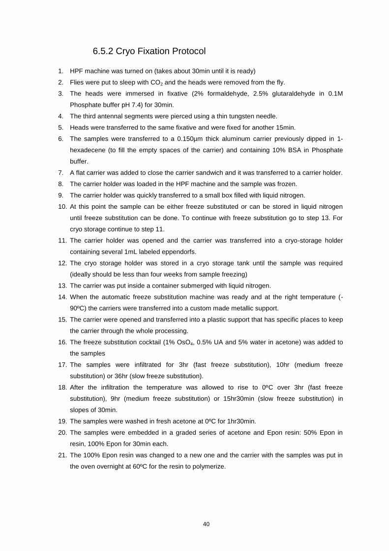
40
6.5.2 Cryo Fixation Protocol
1. HPF machine was turned on (takes about 30min until it is ready)
2. Flies were put to sleep with CO2 and the heads were removed from the fly.
3. The heads were immersed in fixative (2% formaldehyde, 2.5% glutaraldehyde in 0.1M
Phosphate buffer pH 7.4) for 30min.
4. The third antennal segments were pierced using a thin tungsten needle.
5. Heads were transferred to the same fixative and were fixed for another 15min.
6. The samples were transferred to a 0.150µm thick aluminum carrier previously dipped in 1-
hexadecene (to fill the empty spaces of the carrier) and containing 10% BSA in Phosphate
buffer.
7. A flat carrier was added to close the carrier sandwich and it was transferred to a carrier holder.
8. The carrier holder was loaded in the HPF machine and the sample was frozen.
9. The carrier holder was quickly transferred to a small box filled with liquid nitrogen.
10. At this point the sample can be either freeze substituted or can be stored in liquid nitrogen
until freeze substitution can be done. To continue with freeze substitution go to step 13. For
cryo storage continue to step 11.
11. The carrier holder was opened and the carrier was transferred into a cryo-storage holder
containing several 1mL labeled eppendorfs.
12. The cryo storage holder was stored in a cryo storage tank until the sample was required
(ideally should be less than four weeks from sample freezing)
13. The carrier was put inside a container submerged with liquid nitrogen.
14. When the automatic freeze substitution machine was ready and at the right temperature (-
90ºC) the carriers were transferred into a custom made metallic support.
15. The carrier were opened and transferred into a plastic support that has specific places to keep
the carrier through the whole processing.
16. The freeze substitution cocktail (1% OsO4, 0.5% UA and 5% water in acetone) was added to
the samples
17. The samples were infiltrated for 3hr (fast freeze substitution), 10hr (medium freeze
substitution) or 36hr (slow freeze substitution).
18. After the infiltration the temperature was allowed to rise to 0ºC over 3hr (fast freeze
substitution), 9hr (medium freeze substitution) or 15hr30min (slow freeze substitution) in
slopes of 30min.
19. The samples were washed in fresh acetone at 0ºC for 1hr30min.
20. The samples were embedded in a graded series of acetone and Epon resin: 50% Epon in
resin, 100% Epon for 30min each.
21. The 100% Epon resin was changed to a new one and the carrier with the samples was put in
the oven overnight at 60ºC for the resin to polymerize.

41
6.5.3 Randomization of samples Done similarly to described in 6.4.3
6.5.4 Sample selection and sectioning Done similarly to described in 6.4.4
6.5.5 Sample post-staining Done similarly to described in 6.4.5
6.5.6 Sample imaging Done similarly to described in 6.4.6
6.5.7 Sample evaluation Done similarly to described in 6.4.7
6.5.8 Statistical analysis Done similarly to described in 6.4.8
6.6 Materials, Reagents, Equipment and IPE
For this chapter consult appendix, subchapter 10.6.
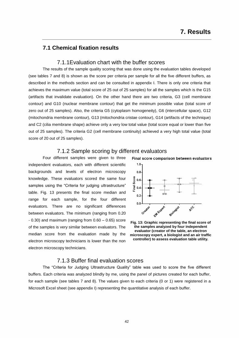
42
7. Results
7.1 Chemical fixation results
7.1.1Evaluation chart with the buffer scores The results of the sample quality scoring that was done using the evaluation tables developed
(see tables 7 and 8) is shown as the score per criteria per sample for all the five different buffers, as
described in the methods section and can be consulted in appendix I. There is only one criteria that
achieves the maximum value (total score of 25 out of 25 samples) for all the samples which is the G15
(artifacts that invalidate evaluation). On the other hand there are two criteria, G3 (cell membrane
contour) and G10 (nuclear membrane contour) that get the minimum possible value (total score of
zero out of 25 samples). Also, the criteria G5 (cytoplasm homogeneity), G6 (intercellular space), G12
(mitochondria membrane contour), G13 (mitochondria cristae contour), G14 (artifacts of the technique)
and C2 (cilia membrane shape) achieve only a very low total value (total score equal or lower than five
out of 25 samples). The criteria G2 (cell membrane continuity) achieved a very high total value (total
score of 20 out of 25 samples).
7.1.2 Sample scoring by different evaluators Four different samples were given to three
independent evaluators, each with different scientific
backgrounds and levels of electron microscopy
knowledge. These evaluators scored the same four
samples using the “Criteria for judging ultrastructure”
table. Fig. 13 presents the final score median and
range for each sample, for the four different
evaluators. There are no significant differences
between evaluators. The minimum (ranging from 0.20
- 0.30) and maximum (ranging from 0.60 – 0.65) score
of the samples is very similar between evaluators. The
median score from the evaluation made by the
electron microscopy technicians is lower than the non
electron microscopy technicians.
7.1.3 Buffer final evaluation scores The “Criteria for Judging Ultrastructure Quality” table was used to score the five different
buffers. Each criteria was analyzed blindly by me, using the panel of pictures created for each buffer,
for each sample (see tables 7 and 8). The values given to each criteria (0 or 1) were registered in a
Microsoft Excel sheet (see appendix I) representing the quantitative analysis of each buffer.
Fig. 13: Graphic representing the final score of the samples analyzed by four independent evaluator (creator of the table, an electron
microscopy expert, a biologist and an air traffic controller) to assess evaluation table utility.

43
The final scores obtained with this method
(which are a ratio - the sum of the score for all the
20 criteria divided by 20) were then used to create
the “Buffer Evaluation Scores” table. Fig. 14
presents the median and range for each buffer, for
the five different samples analyzed per buffer.
Looking at Fig. 14, from all the 25 samples
analyzed (divided by five buffers), only four have
score values above half of the maximum score
(0.5). One corresponds to Cacodylate buffer
(score 0.55) and the other three to PBS buffer
(scores 0.5, 0.60 and 0.65). Also, only one buffer
median hits the 0.5 score corresponding to PBS.
The difference in final score between PBS and
water is statistical significant.
As for descriptive statistics, we can see that the buffer with the lowest minimum is Water (0.2)
and the buffer with the highest maximum is PBS (0.65). The buffers with lowest median are
Cacodylate and Water (both with 0.3) and the buffer with the highest median is PBS (0.5).
7.1.4 General evaluation scores As mentioned above, the final scores
obtained are a sum of the general evaluation scores
and the cilia scores. Fig. 15 shows the general
evaluation scores for each buffer and presents
median and range for each buffer, for the five
different samples analyzed per buffer.
As shown in Fig. 15, from all the 25 samples
analyzed (divided by five buffers), only four have
score values above half of the maximum score (0.5).
One corresponds to PHEM buffer (score 0.53) and
the other three to PBS buffer (scores 0.53, 0.6 and
0.67). Also, only one buffer median is above the 0.5
score corresponding to PBS (0.53). However, there
are no statistically significant differences between
buffers.
As for descriptive statistics, we can see that the buffers with the lowest minimum are both
Phosphate and water (0.2) and the buffer with the highest maximum is PBS (0.67). The buffer with
lowest median is Water (0.27) and the buffer with the highest median is PBS (0.53).
Fig. 14: Graphic representing the final evaluation score of the samples analyzed for the five
different buffers used in the chemical fixation protocol.
Fig. 15: Graphic representing the general evaluation score of the samples analyzed for the
five different buffers used in the chemical fixation protocol.

44
7.1.5 Cilia evaluation scores Fig. 16 shows the cilia evaluation scores for
each buffer. This graphic presents median and range
for each buffer, for the five different samples
analyzed per buffer.
Looking at Fig. 16, from all the 25 samples
analyzed (divided by five buffers), nine have score
values above half of the maximum score (0.5). Three
correspond to Phosphate buffer (scores 0.6, 0.6 and
0.8), two to PHEM buffer (both scores 0.6), one to
Cacodylate (score 0.8) and finally three correspond to
PBS buffer (scores 0.6, 0.8 and 0.8). Two buffer
medians are above the 0.5 score corresponding to
Phosphate (0.6) and to PBS (also 0.6). However,
there are no statistically significant differences
between buffers.
As for descriptive statistics, we can see that the buffers with the lowest minimum are
Phosphate, PHEM and water (0.0) and the buffers with the highest maximum are Phosphate,
Cacodylate and PBS (0.8). The buffer with lowest median is Water (0.2) and the buffer with the
highest median is Phosphate and PBS (0.6).
7.1.6 Panel Analysis Fig. 17 shows the representative pictures of the best cilia score (top row) and the worse cilia
score (bottom row) for each of the five different buffers analyzed. The best and worst cilia score
pictures depict the best and worst cilia scores obtained using the evaluation tables (see appendix
10.1).
Fig. 16: Graphic representing the cilia evaluation score of the samples analyzed for the five
different buffers used in the chemical fixation protocol.
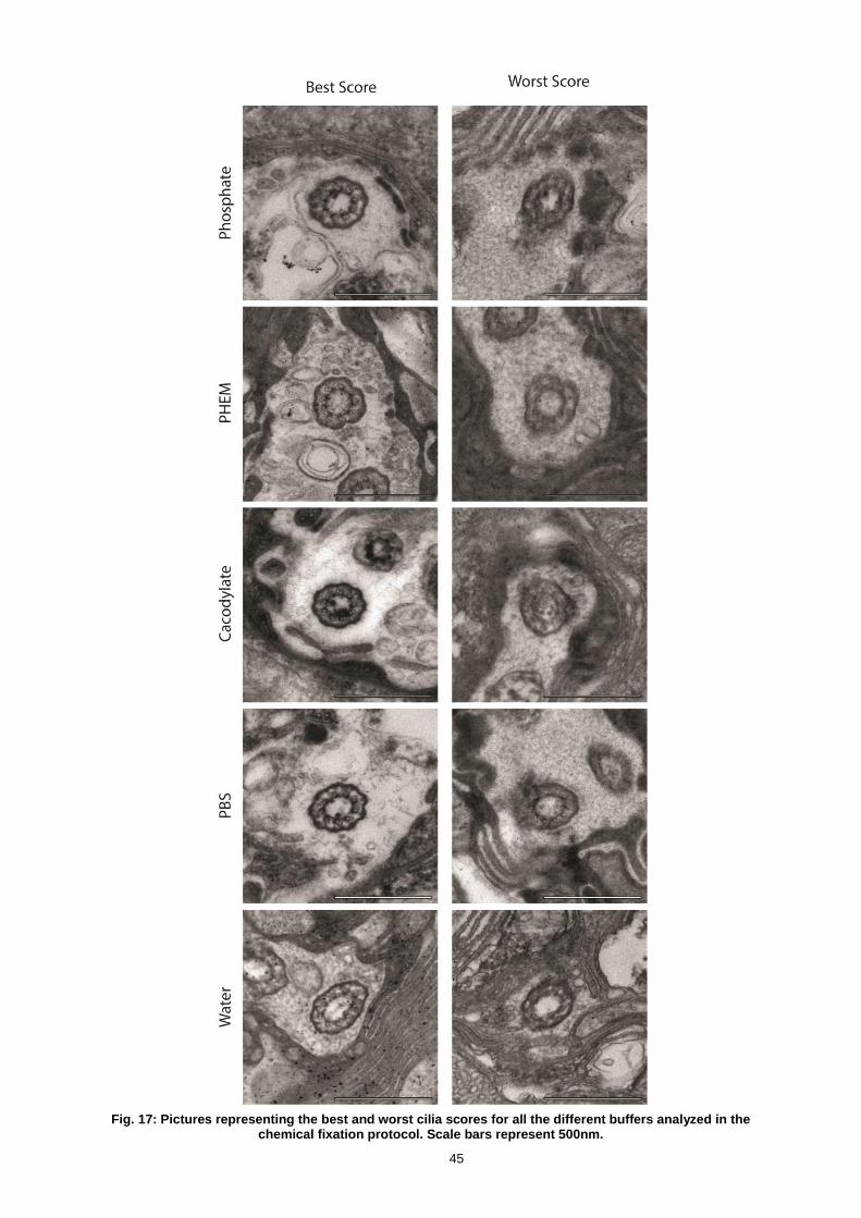
45
Fig. 17: Pictures representing the best and worst cilia scores for all the different buffers analyzed in the chemical fixation protocol. Scale bars represent 500nm.

46
7.2 Cryo fixation results
7.2.1 Evaluation chart with the buffer scores The results of the sample quality scoring that was done using the evaluation tables I
developed (see tables 7 and 8) are shown as the score per criteria per sample for all the three
different freeze substitution times (see appendix II). There are four criteria that achieve the maximum
value per criteria for all the samples, which are the G11 (mitochondria shape), G15 (artifacts that
invalidate evaluation), C1 (cilia membrane continuity) and C2 (cilia membrane shape) in a total score
of six out of six samples. On the other hand there are two criteria, G10 (nuclear membrane contour)
and C4 (y-linkers visibility) that get the minimum possible value (total score of zero out of six samples).
Also, the criteria G2 (cell membrane continuity) and G4 (cell membrane artifacts) achieve a very high
total value (total score of five of six samples).
7.2.2 Freeze substitution final evaluation scores The “Criteria for Judging Ultrastructure Quality” table was
used to analyze the three different freeze substitution times. Each
criteria was analyzed blindly by me, using the panel of pictures
created for each freeze substitution time, for each sample (see
appendix II). The evaluation per sample was done similarly to the
chemically fixed samples (see 7.1.3 Buffer final evaluation scores).
However, since only two samples were analyzed per freeze
substitution time statistical analysis was not done for the cryo
fixation. The points corresponding to each sample score per freeze
substitution time are shown in Fig. 18.
From the six samples analyzed (divided by three freeze
substitution protocols), four have score values above half of the
maximum score (0.5). Two correspond to the fast freeze
substitution (score 0.6 and 0.75), one to the medium freeze substitution (score 0.55) and the other one
to slow freeze substitution (score 0.7). The fast freeze substitution protocol has the highest score from
the three protocols (Fig. 19).
7.2.3 General evaluation scores The final scores obtained are a sum of the general
evaluation scores and the cilia scores. Fig. 19 shows the general
evaluation scores for each freeze substitution.
Looking at Fig. 19, from all the six samples analyzed
(divided by three freeze substitution times), four have score values
above half of the maximum score (0.5). Two correspond to the fast
freeze substitution (score 0.67 and 0.73), one to medium freeze
substitution (score 0.6) and the other one to slow freeze
Fig. 18: Graphic representing the final evaluation score of the
samples analyzed for the three different freeze substitution times used in the cryo fixation protocol.
Fig. 19: Graphic representing the general evaluation score of the samples analyzed for the three
different freeze substitution times used in the cryo fixation protocol.

47
substitution (score 0.73). The fast freeze substitution protocol has the highest score from the three
protocols.
7.2.4 Cilia evaluation scores Fig. 20 shows the cilia evaluation scores for each freeze
substitution.
Looking at Fig. 20, from all the six samples analyzed
(divided by three freeze substitution times), three have score
values above half of the maximum score (0.5). One corresponded
to the fast freeze substitution (score 0.8) and the other two to slow
freeze substitution (both scores 0.6). The fast freeze substitution
protocol has the highest score from the three protocols although with
the range shown all three conditions are scoring about the same.
7.2.5 Panel Analysis Fig. 21 shows the representative pictures of the best cilia score (top row) and the worst cilia
score (bottom row) for each of the three freeze substitution times analyzed. The best and worst cilia
scores pictures depict the best and worst cilia scores obtained using the evaluation tables (see
appendix II). However, it is necessary to take into consideration that besides the fast and medium
freeze substitution protocol showed for best score, all other protocols show ice crystal damage so the
best and worst score pictures may not reflect the true preservation of the tissue.
Fig. 21: Pictures representing of the best and worst scores for all the freeze substitution times analyzed in the cryo fixation protocol. Scale bars represent 500nm.
Fig. 20: Graphic representing the cilia evaluation score of the
samples analyzed for the three different freeze substitution
times used in the cryo fixation protocol.

48
7.3 Chemical vs Cryo fixation
7.3.1 Comparison of the general score between the best and worst buffer and the best and worst freeze substitution protocol Fig. 22 shows the representative
pictures of the best general score (top
row) of all the buffers and freeze
substitution times analyzed and the
worse final score (bottom row) of all
buffers and freeze substitution times
analyzed. The graphic represents the
values of the general score from the
samples represented in the figure.
7.3.2 Comparison of the cilia score between the best and worst buffer and the best and worst freeze substitution protocol Fig. 23 shows the representative
pictures of the best cilia score (top row) of
all the buffers and freeze substitution times
analyzed and the worse cilia score (bottom
row) of all buffers and freeze substitution
times analyzed. The graphic below
represents the values of the cilia score from
the samples represented in the figure.
Fig. 22: On the left: Representative graphic of the best and worse scores in the general evaluation for the samples analyzed for chemical and cryo fixation. On the right: Pictures representative of the values of the
general score from the samples represented in the panel. Scale bars represent 500nm.
Fig. 23: On the left: Representative graphic of the best and worse scores in the cilia evaluation for the samples analyzed for chemical and cryo fixation. On the right: Pictures representative of the values of the cilia score from
the samples represented in the panel. Scale bars represent 500nm.
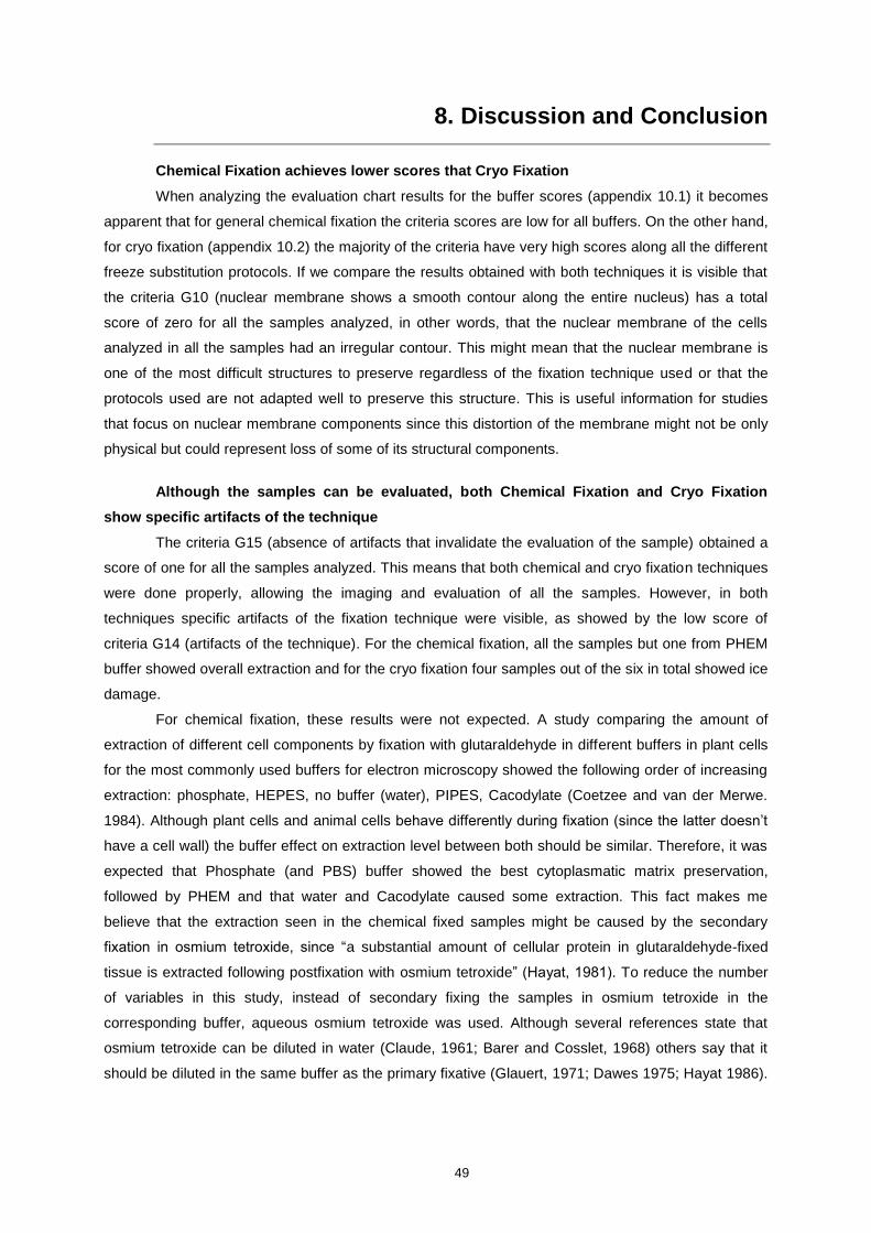
49
8. Discussion and Conclusion
Chemical Fixation achieves lower scores that Cryo Fixation
When analyzing the evaluation chart results for the buffer scores (appendix 10.1) it becomes
apparent that for general chemical fixation the criteria scores are low for all buffers. On the other hand,
for cryo fixation (appendix 10.2) the majority of the criteria have very high scores along all the different
freeze substitution protocols. If we compare the results obtained with both techniques it is visible that
the criteria G10 (nuclear membrane shows a smooth contour along the entire nucleus) has a total
score of zero for all the samples analyzed, in other words, that the nuclear membrane of the cells
analyzed in all the samples had an irregular contour. This might mean that the nuclear membrane is
one of the most difficult structures to preserve regardless of the fixation technique used or that the
protocols used are not adapted well to preserve this structure. This is useful information for studies
that focus on nuclear membrane components since this distortion of the membrane might not be only
physical but could represent loss of some of its structural components.
Although the samples can be evaluated, both Chemical Fixation and Cryo Fixation
show specific artifacts of the technique
The criteria G15 (absence of artifacts that invalidate the evaluation of the sample) obtained a
score of one for all the samples analyzed. This means that both chemical and cryo fixation techniques
were done properly, allowing the imaging and evaluation of all the samples. However, in both
techniques specific artifacts of the fixation technique were visible, as showed by the low score of
criteria G14 (artifacts of the technique). For the chemical fixation, all the samples but one from PHEM
buffer showed overall extraction and for the cryo fixation four samples out of the six in total showed ice
damage.
For chemical fixation, these results were not expected. A study comparing the amount of
extraction of different cell components by fixation with glutaraldehyde in different buffers in plant cells
for the most commonly used buffers for electron microscopy showed the following order of increasing
extraction: phosphate, HEPES, no buffer (water), PIPES, Cacodylate (Coetzee and van der Merwe.
1984). Although plant cells and animal cells behave differently during fixation (since the latter doesn’t
have a cell wall) the buffer effect on extraction level between both should be similar. Therefore, it was
expected that Phosphate (and PBS) buffer showed the best cytoplasmatic matrix preservation,
followed by PHEM and that water and Cacodylate caused some extraction. This fact makes me
believe that the extraction seen in the chemical fixed samples might be caused by the secondary
fixation in osmium tetroxide, since “a substantial amount of cellular protein in glutaraldehyde-fixed
tissue is extracted following postfixation with osmium tetroxide” (Hayat, 1981). To reduce the number
of variables in this study, instead of secondary fixing the samples in osmium tetroxide in the
corresponding buffer, aqueous osmium tetroxide was used. Although several references state that
osmium tetroxide can be diluted in water (Claude, 1961; Barer and Cosslet, 1968) others say that it
should be diluted in the same buffer as the primary fixative (Glauert, 1971; Dawes 1975; Hayat 1986).
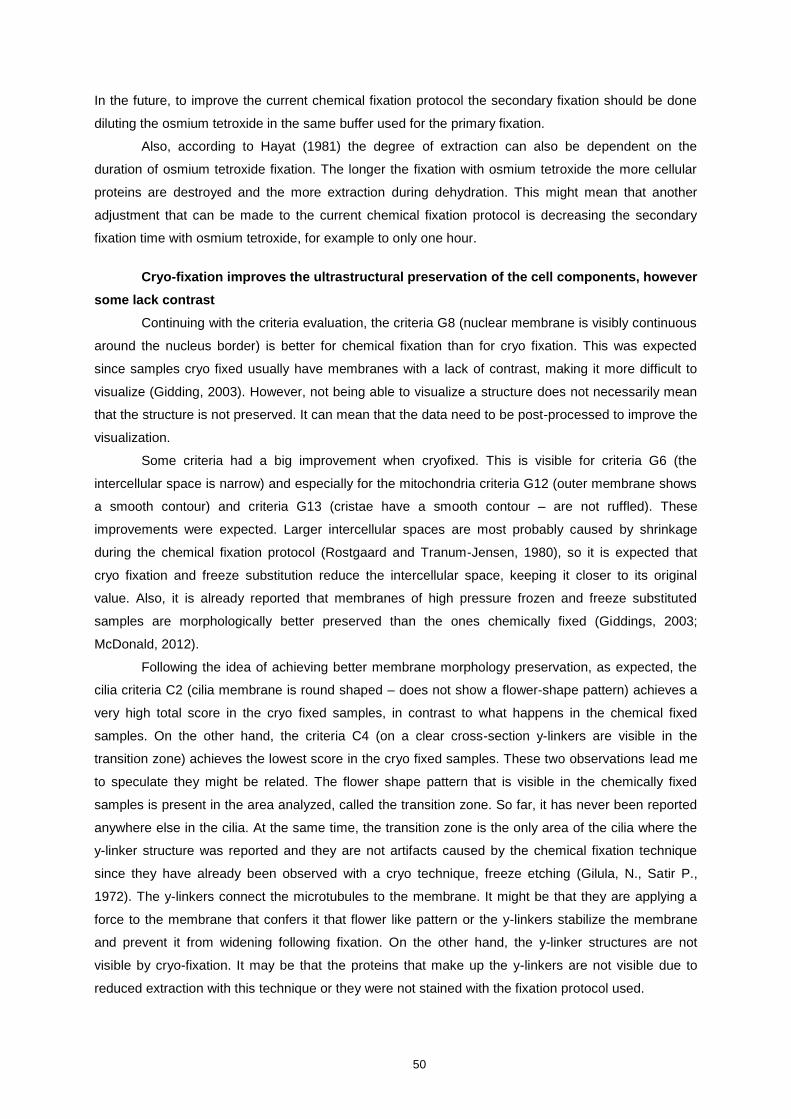
50
In the future, to improve the current chemical fixation protocol the secondary fixation should be done
diluting the osmium tetroxide in the same buffer used for the primary fixation.
Also, according to Hayat (1981) the degree of extraction can also be dependent on the
duration of osmium tetroxide fixation. The longer the fixation with osmium tetroxide the more cellular
proteins are destroyed and the more extraction during dehydration. This might mean that another
adjustment that can be made to the current chemical fixation protocol is decreasing the secondary
fixation time with osmium tetroxide, for example to only one hour.
Cryo-fixation improves the ultrastructural preservation of the cell components, however
some lack contrast
Continuing with the criteria evaluation, the criteria G8 (nuclear membrane is visibly continuous
around the nucleus border) is better for chemical fixation than for cryo fixation. This was expected
since samples cryo fixed usually have membranes with a lack of contrast, making it more difficult to
visualize (Gidding, 2003). However, not being able to visualize a structure does not necessarily mean
that the structure is not preserved. It can mean that the data need to be post-processed to improve the
visualization.
Some criteria had a big improvement when cryofixed. This is visible for criteria G6 (the
intercellular space is narrow) and especially for the mitochondria criteria G12 (outer membrane shows
a smooth contour) and criteria G13 (cristae have a smooth contour – are not ruffled). These
improvements were expected. Larger intercellular spaces are most probably caused by shrinkage
during the chemical fixation protocol (Rostgaard and Tranum-Jensen, 1980), so it is expected that
cryo fixation and freeze substitution reduce the intercellular space, keeping it closer to its original
value. Also, it is already reported that membranes of high pressure frozen and freeze substituted
samples are morphologically better preserved than the ones chemically fixed (Giddings, 2003;
McDonald, 2012).
Following the idea of achieving better membrane morphology preservation, as expected, the
cilia criteria C2 (cilia membrane is round shaped – does not show a flower-shape pattern) achieves a
very high total score in the cryo fixed samples, in contrast to what happens in the chemical fixed
samples. On the other hand, the criteria C4 (on a clear cross-section y-linkers are visible in the
transition zone) achieves the lowest score in the cryo fixed samples. These two observations lead me
to speculate they might be related. The flower shape pattern that is visible in the chemically fixed
samples is present in the area analyzed, called the transition zone. So far, it has never been reported
anywhere else in the cilia. At the same time, the transition zone is the only area of the cilia where the
y-linker structure was reported and they are not artifacts caused by the chemical fixation technique
since they have already been observed with a cryo technique, freeze etching (Gilula, N., Satir P.,
1972). The y-linkers connect the microtubules to the membrane. It might be that they are applying a
force to the membrane that confers it that flower like pattern or the y-linkers stabilize the membrane
and prevent it from widening following fixation. On the other hand, the y-linker structures are not
visible by cryo-fixation. It may be that the proteins that make up the y-linkers are not visible due to
reduced extraction with this technique or they were not stained with the fixation protocol used.
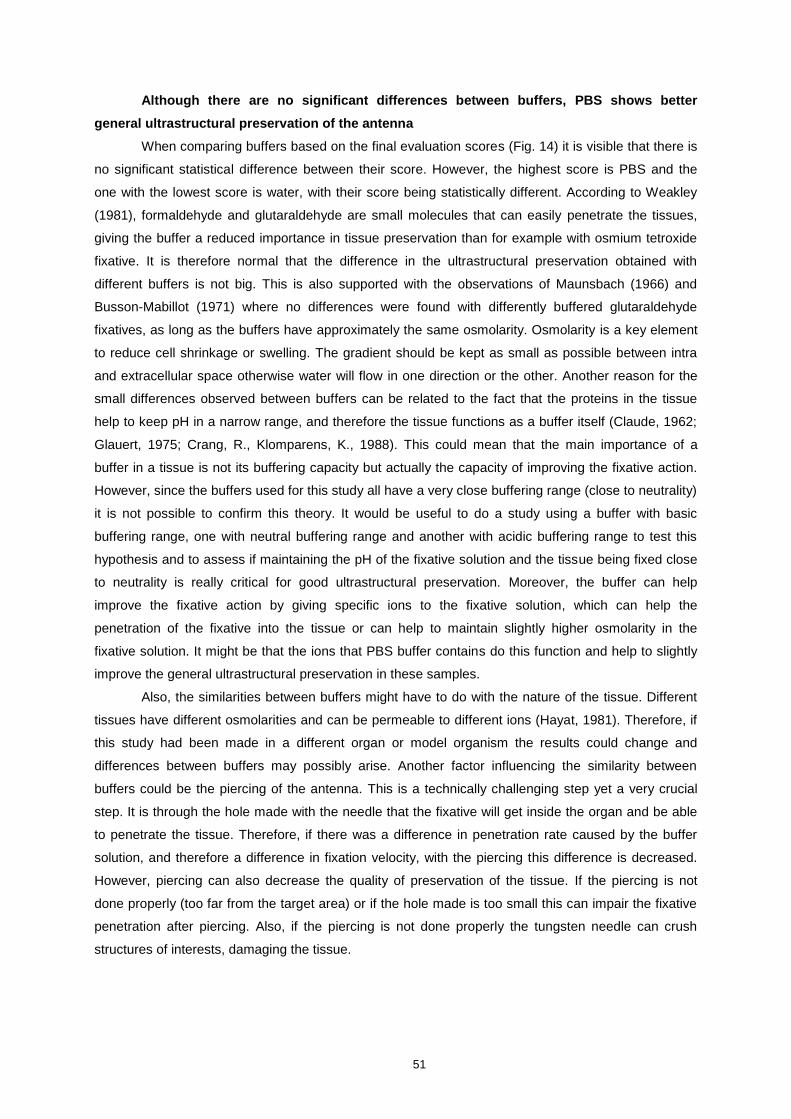
51
Although there are no significant differences between buffers, PBS shows better
general ultrastructural preservation of the antenna
When comparing buffers based on the final evaluation scores (Fig. 14) it is visible that there is
no significant statistical difference between their score. However, the highest score is PBS and the
one with the lowest score is water, with their score being statistically different. According to Weakley
(1981), formaldehyde and glutaraldehyde are small molecules that can easily penetrate the tissues,
giving the buffer a reduced importance in tissue preservation than for example with osmium tetroxide
fixative. It is therefore normal that the difference in the ultrastructural preservation obtained with
different buffers is not big. This is also supported with the observations of Maunsbach (1966) and
Busson-Mabillot (1971) where no differences were found with differently buffered glutaraldehyde
fixatives, as long as the buffers have approximately the same osmolarity. Osmolarity is a key element
to reduce cell shrinkage or swelling. The gradient should be kept as small as possible between intra
and extracellular space otherwise water will flow in one direction or the other. Another reason for the
small differences observed between buffers can be related to the fact that the proteins in the tissue
help to keep pH in a narrow range, and therefore the tissue functions as a buffer itself (Claude, 1962;
Glauert, 1975; Crang, R., Klomparens, K., 1988). This could mean that the main importance of a
buffer in a tissue is not its buffering capacity but actually the capacity of improving the fixative action.
However, since the buffers used for this study all have a very close buffering range (close to neutrality)
it is not possible to confirm this theory. It would be useful to do a study using a buffer with basic
buffering range, one with neutral buffering range and another with acidic buffering range to test this
hypothesis and to assess if maintaining the pH of the fixative solution and the tissue being fixed close
to neutrality is really critical for good ultrastructural preservation. Moreover, the buffer can help
improve the fixative action by giving specific ions to the fixative solution, which can help the
penetration of the fixative into the tissue or can help to maintain slightly higher osmolarity in the
fixative solution. It might be that the ions that PBS buffer contains do this function and help to slightly
improve the general ultrastructural preservation in these samples.
Also, the similarities between buffers might have to do with the nature of the tissue. Different
tissues have different osmolarities and can be permeable to different ions (Hayat, 1981). Therefore, if
this study had been made in a different organ or model organism the results could change and
differences between buffers may possibly arise. Another factor influencing the similarity between
buffers could be the piercing of the antenna. This is a technically challenging step yet a very crucial
step. It is through the hole made with the needle that the fixative will get inside the organ and be able
to penetrate the tissue. Therefore, if there was a difference in penetration rate caused by the buffer
solution, and therefore a difference in fixation velocity, with the piercing this difference is decreased.
However, piercing can also decrease the quality of preservation of the tissue. If the piercing is not
done properly (too far from the target area) or if the hole made is too small this can impair the fixative
penetration after piercing. Also, if the piercing is not done properly the tungsten needle can crush
structures of interests, damaging the tissue.
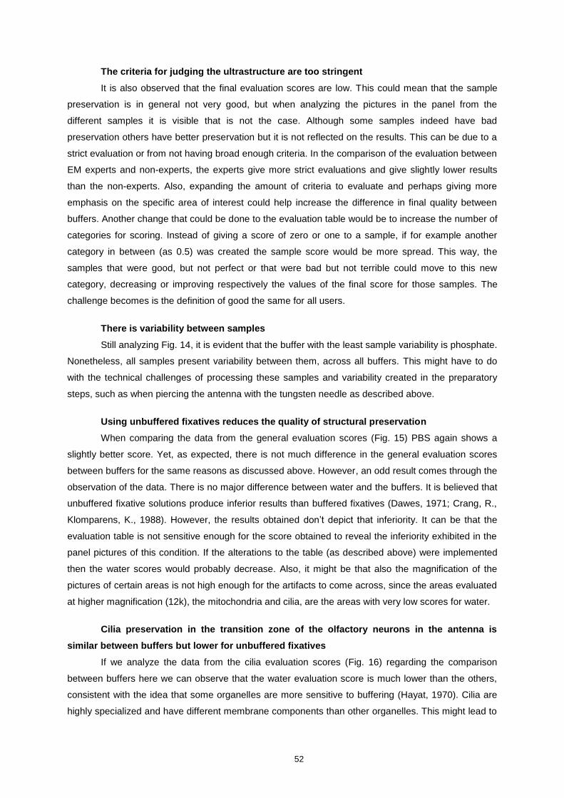
52
The criteria for judging the ultrastructure are too stringent
It is also observed that the final evaluation scores are low. This could mean that the sample
preservation is in general not very good, but when analyzing the pictures in the panel from the
different samples it is visible that is not the case. Although some samples indeed have bad
preservation others have better preservation but it is not reflected on the results. This can be due to a
strict evaluation or from not having broad enough criteria. In the comparison of the evaluation between
EM experts and non-experts, the experts give more strict evaluations and give slightly lower results
than the non-experts. Also, expanding the amount of criteria to evaluate and perhaps giving more
emphasis on the specific area of interest could help increase the difference in final quality between
buffers. Another change that could be done to the evaluation table would be to increase the number of
categories for scoring. Instead of giving a score of zero or one to a sample, if for example another
category in between (as 0.5) was created the sample score would be more spread. This way, the
samples that were good, but not perfect or that were bad but not terrible could move to this new
category, decreasing or improving respectively the values of the final score for those samples. The
challenge becomes is the definition of good the same for all users.
There is variability between samples
Still analyzing Fig. 14, it is evident that the buffer with the least sample variability is phosphate.
Nonetheless, all samples present variability between them, across all buffers. This might have to do
with the technical challenges of processing these samples and variability created in the preparatory
steps, such as when piercing the antenna with the tungsten needle as described above.
Using unbuffered fixatives reduces the quality of structural preservation
When comparing the data from the general evaluation scores (Fig. 15) PBS again shows a
slightly better score. Yet, as expected, there is not much difference in the general evaluation scores
between buffers for the same reasons as discussed above. However, an odd result comes through the
observation of the data. There is no major difference between water and the buffers. It is believed that
unbuffered fixative solutions produce inferior results than buffered fixatives (Dawes, 1971; Crang, R.,
Klomparens, K., 1988). However, the results obtained don’t depict that inferiority. It can be that the
evaluation table is not sensitive enough for the score obtained to reveal the inferiority exhibited in the
panel pictures of this condition. If the alterations to the table (as described above) were implemented
then the water scores would probably decrease. Also, it might be that also the magnification of the
pictures of certain areas is not high enough for the artifacts to come across, since the areas evaluated
at higher magnification (12k), the mitochondria and cilia, are the areas with very low scores for water.
Cilia preservation in the transition zone of the olfactory neurons in the antenna is
similar between buffers but lower for unbuffered fixatives
If we analyze the data from the cilia evaluation scores (Fig. 16) regarding the comparison
between buffers here we can observe that the water evaluation score is much lower than the others,
consistent with the idea that some organelles are more sensitive to buffering (Hayat, 1970). Cilia are
highly specialized and have different membrane components than other organelles. This might lead to

53
different membrane diffusion of the fixative to the interior of the cilia, requiring more buffering function
than other cellular components to protect the structure from the harmful fixative action. Another
interesting finding is that phosphate, Cacodylate and PBS are able to achieve the same high score
(0.8), very close to the maximum possible and PHEM achieves a little less than them.
Extraction of cytoplasmatic components can help to improve the visualization of
certain cellular components
If we analyze the pictures from Fig. 17 we can easily correlate the better scores achieved by
these buffers with the level of extraction they cause in the sample. It seems that the more extracted
the cilia matrix is, the easier it is to visualize the microtubules and the y-linkers. The latter structures
were never visible with PHEM, since this buffer has a much lower extractive action, preserving the cilia
cytoplasm which makes it denser and conferring less contrast with the other structures. This is also a
very interesting finding since it goes against the belief that extraction is always harmful. Obviously that
with extraction comes information loss (Crang, R., Klomparens, K., 1988) but if the structure that we
want to analyze is actually not altered then the greater relative contrast gained with the extraction of
cytoplasmatic matrix can be very helpful, as portrayed in this situation.
Fast Freeze substitution yields good ultrastructural preservation of the antenna
Although this study was more focused on chemical fixation since is the routine technique in
the majority of the electron microscopy laboratories in Portugal, a brief study of cryo fixation was also
one of the goals, since this technique has gained importance over the last years.
Before discussing the results, it is important to emphasize that these conclusions are based on
a very low number of samples, so it is very hard to extrapolate the results. Despite the low number of
samples for the comparison between different freeze substitution times, some interesting results were
observed.
The freeze substitution time that showed the best results in final, general and cilia evaluation
(Figures 19, 20 and 21 respectively) was the fast freeze substitution protocol. This result was
expected since there are protocols for fast freeze substitution in Dm (although for different organs than
the antenna) published showing good results (McDonald, 2012, 2014). This is a very encouraging
result since less time doing freeze substitution implies having results much faster, having less
equipment time being used and spending less technician time therefore decreasing the overall cost of
the technique.
Cryo-fixation methods have a very low sample survival rate
Besides being a very time consuming and expensive protocol, cryo fixing samples achieves a
very low sample survival rate. This means that medium and low freeze substitution time are not
necessarily bad for the overall quality of the samples but only that the samples analyzed were not
preserved. If we take a look at the Fig. 21 we can immediately see that the samples analyzed had ice
damage. In a normal evaluation scenario these samples that are completely damaged by ice formation
should not be used for analysis. However, I wanted to convey the difficulty of this technique and show
how low the survival rate can be. The truth for this technique seems to be that the majority of the

54
samples are badly preserved but the ones that are correctly cryo fixed show a very good
ultrastructural preservation (Fig. 22), as has been already described by many authors.
This bad ultrastructural preservation can be a result of manipulation artifacts prior to high
pressure freezing the sample. The most important step in HPF is sample loading into the specimen
holder (McDonald, 2012). In this protocol this is a step very difficult to perform. First the sample is
slightly fixed (approximately 30min) to allow the piercing of the antenna. After piercing the sample is
transferred to fixative for about 15min. The goal of such a short fixation time is to avoid chemical
fixation artifacts. However, the antenna is hollow inside and therefore 15min might not be enough for
the fixative to penetrate the tissue and fill the empty spaces inside the third segment of the antenna. If
there is still air in the sample during HPF the tissue can collapse and be damaged. One solution for
this problem would be to increase the fixation time after piercing. However, increasing the time of
fixation could lead to chemical fixation artifacts which hinder the goal of cryo fixing the sample:
keeping the sample as close as possible to its native state. One proof that this could happen is visible
in sample one from the protocol of medium freeze substitution. If comparing this sample with the
images of chemically fixed samples or cryo fixed samples it is visible that the sample of medium FS
look more similar to samples chemical fixed. It is likely that this particular sample was kept in fixative
longer after piercing than the other samples. All the samples are pierced sequentially, which means
that the samples that are pierced first will stay in fixative more time that the one pierced last. This
happens since time of fixation after piercing was only started to count after all samples were pierced.
Therefore, one alternative to prevent chemical fixation artifacts would be to leave the sample in buffer
after piercing instead of fixative. This way, the buffer has the opportunity to fill the empty spaces inside
the antenna and chemical fixation artifacts will be avoided.
To identify the real morphology of a cell component it is necessary to combine
chemical and cryo-fixation techniques
Analyzing the results from the cilia evaluation (Fig. 23) for both techniques we can see that
both achieve the same maximum score (0.8). This means that both techniques have their own
advantages. In the case of chemical fixation, although we have some artifacts like the membrane
contour having a flower shape pattern, we can see the y-linker structures that are not visible by cryo
fixation. However, cryo fixation preserves much better the cilia membrane maintaining it round.
Therefore, what we can conclude from this result is that to fully be able to analyze the ultrastructure of
a cell or a cell component, the best is to combine several techniques and compare specimen
morphologies from different fixation techniques. This is the best way of obtaining reliable
morphological, biochemical and physiological information, for EM studies but can be used as well as a
general rule for all biomedical research techniques (Crang, R., Klomparens, K., 1988).
Otherwise, there is a risk of taking erroneous conclusions from the sample observation like the
case of the bacterial “mesosome”, a membranous structure found in electron micrographs of
chemically processed gram positive bacteria. This structure is actually an artifact of chemical fixation
that was never found in cryo fixation studies (Silva et al, 1976). This example illustrates why it is
important to know what is the aim of each study and to understand how each technique can contribute
to achieve that goal and which artifacts each technique can introduce to the sample.

55
Conclusion
This study gives some insights on the contribution of each method of fixation (chemical and
cryo) to preserve the ciliary structure on the third segment of the Drosophila antenna and what kind of
artifacts arise from each preservation technique. Also, having an evaluation table that summarizes the
desirable characteristics of a sample processed for electron microscopy observation helps to
understand what to look for in the sample when looking for artifacts specific for each technique. It is
also helpful to have a tool that helps to compare between samples and even between techniques not
only qualitatively but also in a quantitative way. As shown here, a huge amount of information can be
extracted when the samples are analyzed this way and this evaluation table has shown to be a
valuable tool not only for experts in electron microscopy but also for people without any background in
the area that might want to start doing some work in this field.
As a final remark I consider this to be a very useful study. It raises the question of what is the
true action of a buffer in a fixative solution, since until now not much is known and discussed regarding
this subject. It would be of great importance if in the future someone would address this question in a
detailed chemical analysis. Also it allowed me to assess the chemical fixation protocol that preserves
better the structures my research group is interested in studying and gave me the opportunity to work
with a new technique (cryo fixation) from which I was able to apply a protocol that provides good
ultrastructural preservation. Also, this might be useful to investigate further the ultrastructure of cilia in
Drosophila melanogaster’s antenna and maybe incorporate it in other studies such as immune
detection of ciliary proteins in the transition zone.
Last but not the least, from this study arises a new tool, an evaluation table for judging
ultrastructure. This table might be very useful since it can be adapted to whatever sample or criteria
being analyzed and it can be specified accordingly to a structure of interest. This can be applied not
only for my routine in the laboratory to assess the quality of the samples I will work with, but also for
everyone that is interested in standardizing new protocols, comparing techniques or even for routine
quality control in electron microscopy facilities.
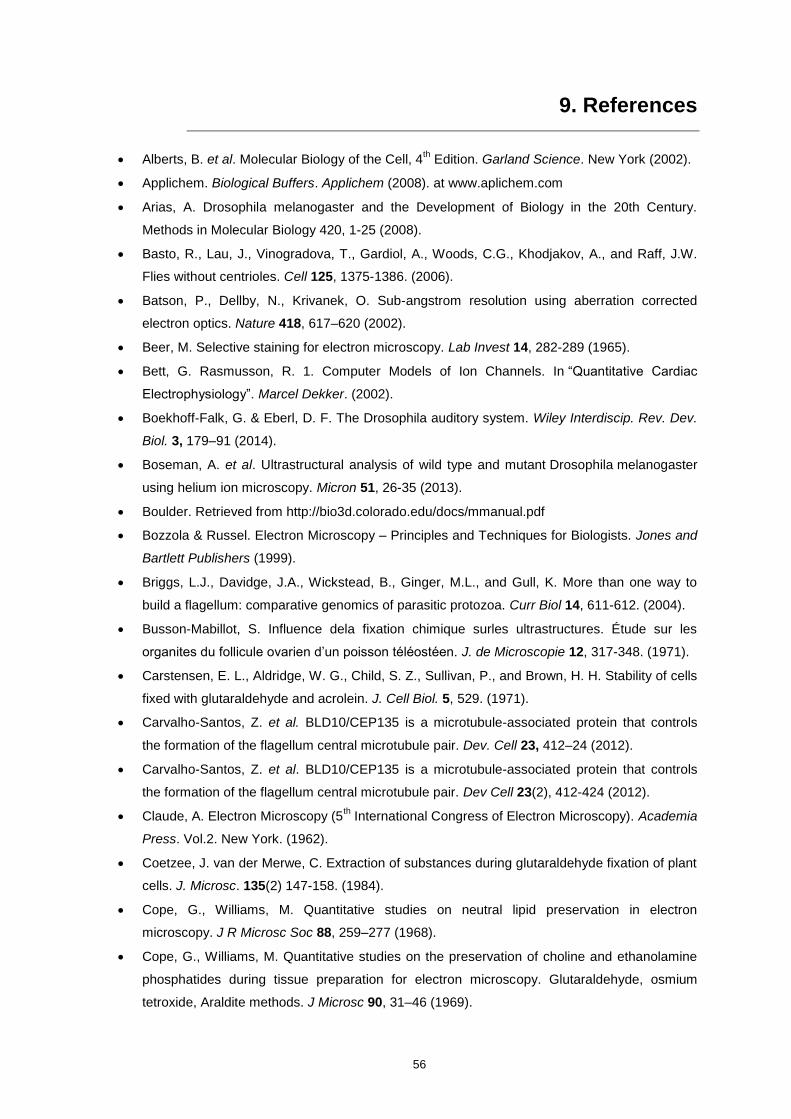
56
9. References
Alberts, B. et al. Molecular Biology of the Cell, 4th Edition. Garland Science. New York (2002).
Applichem. Biological Buffers. Applichem (2008). at www.aplichem.com
Arias, A. Drosophila melanogaster and the Development of Biology in the 20th Century.
Methods in Molecular Biology 420, 1-25 (2008).
Basto, R., Lau, J., Vinogradova, T., Gardiol, A., Woods, C.G., Khodjakov, A., and Raff, J.W.
Flies without centrioles. Cell 125, 1375-1386. (2006).
Batson, P., Dellby, N., Krivanek, O. Sub-angstrom resolution using aberration corrected
electron optics. Nature 418, 617–620 (2002).
Beer, M. Selective staining for electron microscopy. Lab Invest 14, 282-289 (1965).
Bett, G. Rasmusson, R. 1. Computer Models of Ion Channels. In “Quantitative Cardiac
Electrophysiology”. Marcel Dekker. (2002).
Boekhoff-Falk, G. & Eberl, D. F. The Drosophila auditory system. Wiley Interdiscip. Rev. Dev.
Biol. 3, 179–91 (2014).
Boseman, A. et al. Ultrastructural analysis of wild type and mutant Drosophila melanogaster
using helium ion microscopy. Micron 51, 26-35 (2013).
Boulder. Retrieved from http://bio3d.colorado.edu/docs/mmanual.pdf
Bozzola & Russel. Electron Microscopy – Principles and Techniques for Biologists. Jones and
Bartlett Publishers (1999).
Briggs, L.J., Davidge, J.A., Wickstead, B., Ginger, M.L., and Gull, K. More than one way to
build a flagellum: comparative genomics of parasitic protozoa. Curr Biol 14, 611-612. (2004).
Busson-Mabillot, S. Influence dela fixation chimique surles ultrastructures. Étude sur les
organites du follicule ovarien d’un poisson téléostéen. J. de Microscopie 12, 317-348. (1971).
Carstensen, E. L., Aldridge, W. G., Child, S. Z., Sullivan, P., and Brown, H. H. Stability of cells
fixed with glutaraldehyde and acrolein. J. Cell Biol. 5, 529. (1971).
Carvalho-Santos, Z. et al. BLD10/CEP135 is a microtubule-associated protein that controls
the formation of the flagellum central microtubule pair. Dev. Cell 23, 412–24 (2012).
Carvalho-Santos, Z. et al. BLD10/CEP135 is a microtubule-associated protein that controls
the formation of the flagellum central microtubule pair. Dev Cell 23(2), 412-424 (2012).
Claude, A. Electron Microscopy (5th International Congress of Electron Microscopy). Academia
Press. Vol.2. New York. (1962).
Coetzee, J. van der Merwe, C. Extraction of substances during glutaraldehyde fixation of plant
cells. J. Microsc. 135(2) 147-158. (1984).
Cope, G., Williams, M. Quantitative studies on neutral lipid preservation in electron
microscopy. J R Microsc Soc 88, 259–277 (1968).
Cope, G., Williams, M. Quantitative studies on the preservation of choline and ethanolamine
phosphatides during tissue preparation for electron microscopy. Glutaraldehyde, osmium
tetroxide, Araldite methods. J Microsc 90, 31–46 (1969).

57
Crang, R., Klomparens, K., Artifacts in Biological Electron Microscopy. Springer (1988).
Dahl, R. and L.A. Staehelin. High pressure freezing for the preservation of biological structure:
theory and practice. J. Electron Microsc. Tech. 13:165-174, (1989).
Davies, G. E., and Stark, G. R. Use of dimethylsuberimidate, a crosslinking reagent in
studying the subunit structure of oligomeric proteins. Proc. Natl. Acad.. 66, 651. (1970).
Dawes, C. Biological techniques in electron microscopy. Barnes & Noble. (1971).
Doggenweiler, C. F., and Heuser, J. E. Ultrastructure of the prawn nerve sheaths: role of
fixative and osmotic pressure in vesiculation of thin cytoplasmic laminae. J. Cell Biol. 34, 407-
420 (1967).
Doughty, M. Influence of initial fixation protocol on the appearance of primary cilia on the
rabbit corneal endothelial cell apical surface as assessed by scanning electron microscopy.
Cell Biology International 28, 131-137. (2004).
Dubochet, J. The physics of rapid cooling and its implications for cryoimmobilization of cells.
Meth Cell Biol 79, 7–21 (2007).
Dykstra, M. & Reuss, L. Biological Electron Microscopy - Theory, Techniques, and
Troubleshooting. Springer, (2003).
Eberl, D. & Boekhoff-Falk, G. Development of Johnston’s organ in Drosophila. Int. J. Dev. Biol.
51, 679–687 (2007).
Egerton, R. Physical Principles of Electron Microscopy. Springer, (2005).
Eisenberg, B. R., and Mobley, Â. Á. Size changes in single muscle fibers during fixation and
embedding. Tissue Cell 7, 383. (1975).
Ellis, K.J. & Morrison, J.F. Methods Enzymol. 87, 405-426 (1982).
Enjolras, C., Thomas, J., Chhin, B., Cortier, E., Duteyrat, J.L., Soulavie, F., Kernan, M.J.,
Laurencon, A., and Durand, B. Drosophila chibby is required for basal body formation and
ciliogenesis but not for Wg signaling. J Cell Biol 197, 313-325 (2012).
Ericsson, J. L. E., Saldino, A. J., and Trump, B. F. Electron microscopic observations of the
influence of different fixatives on the appearance of cellular ultrastructure. Zellforsch.Mikrosk.
Anat. 66, 161-165 (1965).
Fahimi, H. D., and Drochmans, P. Essais de standardisation de la fixation au glutaraldehyde.
II. Influence des concentrations en aldehyde et de l'osmolalite. J. Microsc. 4, 737. (1965).
Fortin, M. O Processo de Investigação: Da concepção à realização (2ªEdição). Lusociência,
Loures (2000).
Giddings, T. Freeze-substitution protocols for improved visualization of membranes in high-
pressure frozen samples. J Microsc 212, 53-61 (2003).
Glauert, A. Fixation, Dehydration and Embedding of biological specimens. North-Holland
(1975).
Good, N. E. et al. Hydrogen ion buffers for biological Research. Biochemistry 5, 467–477
(1966).
Green, E. W. & Giorgini, F. Choosing and using Drosophila models to characterize modifiers
of Huntington’s disease. Biochem. Soc. Trans. 40, 739–45 (2012).

58
Griffiths, G. 2006. Electron Microscopy in Cell Biology. Reviews in Cell Biology and Molecular
Medicine. (Wiley Online Library, 2002)
Hackenbrock, C.Ultrastructural bases for metabolically linked mechanical activity in
mitochondria. II. Electron transport-linked ultrastructural transformations in mitochondria. J.
Cell Biol. 37, 345. (1968).
Hayat, M. Fixation for Electron Microscopy. Acad. Press (1981).
Hayat, M. Principles and techniques of electron microscopy: biological applications, 4th ed.
Cambridge University Press, Cambridge. (2000).
Heller, J., Ostwald, T. J., and Bok, D. The osmotic behavior of rod photoreceptor outer
segment discs. J. Cell Biol. 48, 633. (1971).
http://www.microscopyu.com/articles/formulas/formulasresolution.html
Humbel B, Müller M. Freeze substitution and low temperature embedding. In “The science of
biological specimen preparation 1985”. J.J Wolosewick Ed. 175-183 (1986).
Humbel, B., Marti, T., Müller, M. Improved structural preservation by combining freeze
substitutuion and low temperature embedding. Beitr Elektronenmikroskop Direktabb Oberfl 16,
585–594 (1983).
Jana, S. C., Girotra, M. & Ray, K. Heterotrimeric kinesin-II is necessary and sufficient to
promote different stepwise assembly of morphologically distinct bipartite cilia in Drosophila
antenna. Mol. Biol. Cell 22, 769–81 (2011).
Jana, S. C., Marteil, G. & Bettencourt-Dias, M. Mapping molecules to structure: unveiling
secrets of centriole and cilia assembly with near-atomic resolution. Curr. Opin. Cell Biol. 26,
96–106 (2014).
Jard, S., Bourget, J., Carasso, N., and Favard, P. Action des fixatives sen la perméabilité et
l'ultrastructure de la vessie de grenouille. J. Microsc. 5, 31. (1966).
Jost, P. C , Brooks, U. J., and Griffith, Ï. H. Fluidity of phospholipid bilayers and membranes
after exposure to osmium tetroxide and glutaraldehyde. J. Mol. Biol. 76, 313. (1973).
Kellenberger, E., et al. Artefacts and morphological changes during chemical Wxation. J
Microsc 168, 181–201 (1992).
Konwinski, M., Abramczuk, J., Baranska, W., and Szymkowiak, W. Size changes of mouse
ova during preparation for morphometric studies in the electron microscope. Histochemistry
42, 315. (1974)
Kuo, J. Electron Microscopy - Methods and Protocols. Humana Press, (2014).
Latta, H. Hartmann, J. Use of a glass edge in thin sectioning for electron microscopy. Proc
Soc Exp Biol Med.74 (2): 436–439 (1950).
Lepe-Zuniga JL, Zigler JS, Gery I. "Toxicity of light-exposed Hepes media". J. Immunol.
Methods 103(1) 145 (1987).
Lodish, H. et al. Molecular Cell Biology, 4th Edition. W. H. Freeman. New York (2000).
Luft, J. Improvements in epoxy resin embedding methods. J Biophys Biochem Cytol 9, 409–
414 (1961).

59
Martin, F. et al. Elements of olfactory reception in adult Drosophila melanogaster. Anat
Rec(Hoboken) 296, 1477-88 (2013).
Maunsbach, A. Afzelius, B. Biomedical Electron Microscopy. Academic Press. USA. (1966)
McDonald, K. et al. “Tips and Tricks” for High Pressure Freezing of Model Systems. Methods
in Cell Biology. 96. 671-693. (2010).
McDonald, K. et al. Preparation of Drosophila Specimens for Examination by Transmission
Electron Microscopy. Cold Spring Harbor Protocols 10, 510-515. (2012).
McDonald, K. et al. Recent advances in high-pressure freezing: equipment- and specimen-
loading methods. Methods Mol Biol, 369, 143-173, (2007).
McDonald, K. et al. Transmission Electron Microscopy of Thin Sections of Drosophila: High-
Pressure Freezing and Freeze-Substitution. Cold Spring Harbor Protocols 10, 1044-1048.
(2012).
McDonald, K. Out with the old and in with the new: rapid specimen preparation procedures for
electron microscopy of sectioned biological material. Protoplasma 251, 429–48 (2014).
Meryman, H. Cryopreservation of living cells: principles and practice. Transfusion, 47(5), 935-
945, (2007).
Mohan, C. Buffers: A guide for the preparation and use of buffers in biological systems. EDM
Biosciences, Inc., (2003).
Moor, H. "Theory and practice of high pressure freezing." Cryotechniques in biological
electron microscopy. Springer-Verlag. Heidelberg (1987).
Moor, H., et al. A new freezing-ultramicrotome. J Biophys Biochem Cytol 10, 1–13 (1961).
Morphew, M. K. Practical Methods in High- Pressure Freezing, Freeze-Substitution,
Embedding and Immunocytochemistry for Electron Microscopy, (2002).
Moussian, B., Schwarz, H., Bartoszewski, S. & Nüsslein-Volhard, C. Involvement of chitin in
exoskeleton morphogenesis in Drosophila melanogaster. J. Morphol. 264, 117–30 (2005).
Muhlethaler, K. History of freeze-etching. In: Benedetti L, Favard P (eds) Freeze-etching
techniques and applications. Societe Francaise de Microscopie Electronique, Paris, pp 1–10
(1973).
Müller, H. Die Ausmessung der Tiefe übermikroskopischer Objekte. Kolloid-Z 99, 6–28 (1942).
Palade, G. A study of fixation for electron microscopy. J ExpMed 95, 285–298 (1952).
Palade, G., Porter, K. Studies on the endoplasmic reticulum. Its identification in cells in situ. J
Exp Med 100, 641–656 (1954).
Pandey, U. B. & Nichols, C. D. Human Disease Models in Drosophila melanogaster and the
Role of the Fly in Therapeutic Drug Discovery. Pharmacol. Rev. 63, 411–436 (2011).
Pandithage, R. Brief Introduction to Contrasting for EM Sample Preparation. Leica Contrast
Manual. (2013).
Pentilla, A. Kalimo, H. Trump, B.F. Influence of glutaraldehyde and/or osmium tetroxide on cell
volume, ion content, mechanical stability, and membrane permeability of Ehrlich ascites tumor
cells. J Cell Biol 63, 197-214 (1974).
60
Rasmussen, N. Picture control: The Electron Microscope and the Transformation of American
Biology, 1940-1959. Stanford University Press, Stanford. (1997).
Robertson, J. D. The ultrastructure of cell membranes and their derivatives. Biochem. Soc.
Symp. 16, 3. (1959).
Robinson, D.G et al. Methods of Preparation for Electron Microscopy – An introduction for the
biomedical sciences. Springer (1987).
Rostgaard, J., and Tranum-Jensen, J. A procedure for minimizing cellular shrinkage in
electron microscope preparation: A quantitative study on frog gallbladder. J. Microsc. (Oxford)
119, 213. (1980).
Sabatini, D. D., Miller, F., and Barrnett, R. J. Aldehyde fixation for morphological and enzyme
histochemical studies with the electron microscope. J. Histochem. Cytochem. 12, 57. (1964).
Sabatini, D., Bensch, K., Barrnett, R. Cytochemistry and electron microscopy. The
preservation of cellular ultrastructure and enzymic activity by aldehyde fixation. J Cell Biol 17,
19–58 (1963).
Sanbhag, S. et al. Atlas of olfactory organs of Drosophila melanogaster 1. Types, external
organization, innervation and distribution of olfactory sensila. International Journal of Insect
Morphology and Embryology 28, 377-397 (1999).
Sanbhag, S. et al. Atlas of olfactory organs of Drosophila melanogaster 2. Internal
organization and cellular architecture of olfactory sensilla. International Arthropod Structure &
Development 29, 211-229 (2000).
Schiff, R. I. & Gennaro, J. F. The Role of the Buffer in the Fixation of Biological Specimens for
Transmission and Scanning Electron Microscopy. Scanning 2, 135–148 (1979).
Schliwa, M. Blerkom, J. Structural interaction of cytoskeletal components. The Journal of Cell
Biology 90(1) 222-235 (1981).
Scopes, R. Protein Purification - Principles and Practice. Springer (1994).
Scott, J. Routine solutions we use in our laboratory. Retrieved from:
http://www.heuserlab.wustl.edu/procedures/routinesolutions.shtml
SmartBuffer (2014). Retrieved from:
http://www.medicago.se/sites/default/files/pdf/productsheets/PBS_Buffer_v._01.pdf
Sosinsky, G. et al. The combination of chemical fixation procedures with high pressure
freezing and freeze substitution preserves highly labile tissue ultrastructure for electron
tomography applications. J Struct Biol, 161(3), 359-371, (2008).
Steere, R. Electron microscopy of structural detail in frozen biological specimens. J Biophy
Biochem Cytol 3, 45–60 (1957).
Stocker, R. The organization of the chemosensory system in Drosophila melanogaster: a
review. Cell tissue Res. 275, 3-26 (1994).
Studer, D et al, Electron microscopy of high pressure frozen samples: bridging the gap
between cellular ultrastructure and atomic resolution. Histochem Cell Biol, 130(5), 877-889,
(2008).
61
Studer, D., Hennecke, H., Müller, M. High pressure freezing of soybean nodules leads to an
improved preservation of ultrastructure. Planta 188, 155–163 (1992).
Studer, D., Humbel, B. M. & Chiquet, M. Electron microscopy of high pressure frozen
samples: bridging the gap between cellular ultrastructure and atomic resolution. Histochem.
Cell Biol. 130, 877–89 (2008).
Todi, S. V, Sharma, Y. & Eberl, D. F. Anatomical and molecular design of the Drosophila
antenna as a flagellar auditory organ. Microsc. Res. Tech. 63, 388–399 (2004).
Tormey, J. M. Differences in membrane configuration between osmium tetroxide-fixed and
glutaraldehyde-fixed ciliary epithelium. J. Cell Biol. 23, 658. (1964).
Trump, B. F. & Ericsson, J.L. The effect of the fixative solution on the ultrastructure of cells
and tissues. Lab Invest 14, 1245-1323 (1965).
Vincensini, L., Blisnick, T. & Bastin, P. 1001 Model Organisms To Study Cilia and Flagella.
Biol. cell 103, 109–30 (2011).
Wang, Y. Utility of Insects for Studying Human Pathogens and Evaluating New Antimicrobial
Agents. Yellow Biotechnology. 135, 1-25 (2013).
Waters, A. Beales, P., Ciliopathies: an expanding disease spectrum. Pedriatr Nephrol 26(7),
1039-1056. (2011).
Weakley, B. A beginner's handbook in biological transmission electron microscopy. Churchill
Livingstone, New York (1981).
White, D., et al The chemical nature of osmium tetroxide fixation and staining of membranes
by X-ray photoelectron spectroscopy. Biochim Biophys Acta 436, 577–592 (1976).
Wilson, J. M. Gantt charts: A centenary appreciation. Eur. J. Oper. Res. 149, 430–437 (2003).
Wood, R.L. & Luft, J.H. The influence of the buffer systems on fixation with OsO4. J
Ultrastructure Res 12, 22-45 (1965).
Zuber, B. et al. The mammalian central nervous synaptic cleft contains a high density of
periodically organized complexes. Proc Natl Acad Sci USA 102, 19192–19197 (2005).
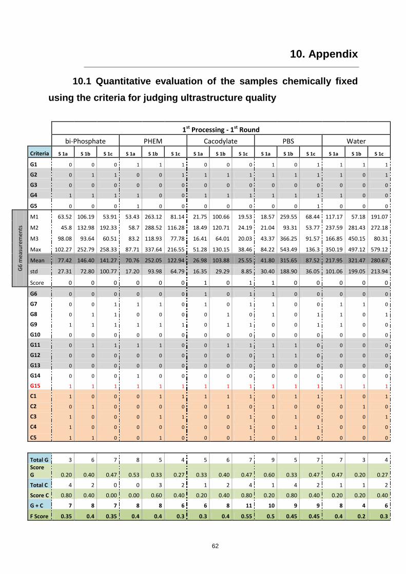
62
10. Appendix
10.1 Quantitative evaluation of the samples chemically fixed
using the criteria for judging ultrastructure quality
1st Processing - 1st Round
bi-Phosphate PHEM Cacodylate PBS Water
Criteria S 1a S 1b S 1c S 1a S 1b S 1c S 1a S 1b S 1c S 1a S 1b S 1c S 1a S 1b S 1c
G1 0 0 0 1 1 1 0 0 0 1 0 1 1 1 1
G2 0 1 1 0 0 1 1 1 1 1 1 1 1 0 1
G3 0 0 0 0 0 0 0 0 0 0 0 0 0 0 0
G4 1 1 1 1 0 0 1 1 1 1 1 1 1 0 0
G5 0 0 0 1 0 0 0 0 0 0 0 1 0 0 0
G6
mea
sure
men
ts
M1 63.52 106.19 53.91 53.43 263.12 81.14 21.75 100.66 19.53 18.57 259.55 68.44 117.17 57.18 191.07
M2 45.8 132.98 192.33 58.7 288.52 116.28 18.49 120.71 24.19 21.04 93.31 53.77 237.59 281.43 272.18
M3 98.08 93.64 60.51 83.2 118.93 77.78 16.41 64.01 20.03 43.37 366.25 91.57 166.85 450.15 80.31
Max 102.27 252.79 258.33 87.71 337.64 216.55 51.28 130.15 38.46 84.22 543.49 136.3 350.19 497.12 579.12
Mean 77.42 146.40 141.27 70.76 252.05 122.94 26.98 103.88 25.55 41.80 315.65 87.52 217.95 321.47 280.67
std 27.31 72.80 100.77 17.20 93.98 64.79 16.35 29.29 8.85 30.40 188.90 36.05 101.06 199.05 213.94
Score 0 0 0 0 0 0 1 0 1 1 0 0 0 0 0
G6 0 0 0 0 0 0 1 0 1 1 0 0 0 0 0
G7 0 0 1 1 1 0 1 0 1 1 0 0 1 1 0
G8 0 1 1 0 0 0 0 1 0 1 0 1 1 0 1
G9 1 1 1 1 1 1 0 1 1 0 0 1 1 0 0
G10 0 0 0 0 0 0 0 0 0 0 0 0 0 0 0
G11 0 1 1 1 1 0 0 1 1 1 1 0 0 0 0
G12 0 0 0 0 0 0 0 0 0 1 1 0 0 0 0
G13 0 0 0 0 0 0 0 0 0 0 0 0 0 0 0
G14 0 0 0 1 0 0 0 0 0 0 0 0 0 0 0
G15 1 1 1 1 1 1 1 1 1 1 1 1 1 1 1
C1 1 0 0 0 1 1 1 1 1 0 1 1 1 0 1
C2 0 1 0 0 0 0 0 1 0 1 0 0 0 1 0
C3 1 0 0 0 1 1 0 0 1 0 1 0 0 0 1
C4 1 0 0 0 0 0 0 0 1 0 1 1 0 0 0
C5 1 1 0 0 1 0 0 0 1 0 1 0 0 0 0
Total G 3 6 7 8 5 4 5 6 7 9 5 7 7 3 4
Score G 0.20 0.40 0.47 0.53 0.33 0.27 0.33 0.40 0.47 0.60 0.33 0.47 0.47 0.20 0.27
Total C 4 2 0 0 3 2 1 2 4 1 4 2 1 1 2
Score C 0.80 0.40 0.00 0.00 0.60 0.40 0.20 0.40 0.80 0.20 0.80 0.40 0.20 0.20 0.40
G + C 7 8 7 8 8 6 6 8 11 10 9 9 8 4 6
F Score 0.35 0.4 0.35 0.4 0.4 0.3 0.3 0.4 0.55 0.5 0.45 0.45 0.4 0.2 0.3

63
1st Processing - 2nd Round 2nd Processing
bi-Phos PHEM Caco PBS H20 bi-Phos PHEM Caco PBS H20
Criteria S 2 S 2 S 2 S 2 S 2 S 3 S 3 S 3 S 3 S 3
Total
G1 0 0 0 1 0 1 0 0 0 0
10 out of 25
G2 1 1 0 1 1 1 1 1 1 1
20 out of 25
G3 0 0 0 0 0 0 0 0 0 0
0 out of 25
G4 0 1 0 1 1 1 0 1 1 0
17 out of 25
G5 0 0 0 1 0 1 0 0 0 0
4 out of 25
G6
mea
sure
men
ts
M1 37.88 103.2 66.76 129.6
5 300.8
9 208.01 106.38 80.82 40.1
6 93.58
M2 57.82 48.19 66.76 86.54 203.8
9 183.35 42 58.61 15.0
2 46.51
M3 19.61 38.46 60.01 163.1
8 100.7
6 107.78 272.32 57.6 16.5
4 126.52
Max 82.84 213.73 160.5
4 265.9
5 505.9
1 363.87 333.47 120.31 40.4
3 130.99
Mean 49.54 100.90 88.52 161.3
3 277.8
6 215.75 188.54 79.34 28.0
4 99.40
std 27.14 80.44 48.12 76.48 172.6
0 107.56 136.93 29.34 14.1
7 39.01 Score 0 0 0 0 0 0 0 0 1 0
G6 0 0 0 0 0 0 0 0 1 0
4 out of 25
G7 1 0 1 1 1 1 1 0 1 1
16 out of 25
G8 0 1 1 1 0 0 0 1 1 1
13 out of 25
G9 1 0 0 0 0 0 1 0 1 0
13 out of 25
G10 0 0 0 0 0 0 0 0 0 0
0 out of 25
G11 1 1 1 1 1 0 1 1 1 0
16 out of 25
G12 0 0 0 1 0 0 0 0 0 0
3 out of 25
G13 0 0 0 1 0 0 0 0 0 0
1 out of 25
G14 0 0 0 0 0 0 0 0 0 0
1 out of 25
G15 1 1 1 1 1 1 1 1 1 1
25 out of 25
C1 1 0 1 1 1 1 1 1 1 0
18 out of 25
C2 0 0 1 0 0 0 0 0 0 0
5 out of 25
C3 1 0 0 1 0 1 1 0 1 0
11 out of 25
C4 0 0 0 0 0 0 0 0 1 0
5 out of 25
C5 1 0 0 1 0 1 1 0 1 0
10 out of 25
Total G 5 5 4 10 5 6 5 5 8 4
Score G 0.33 0.33 0.27 0.67 0.33 0.40 0.33 0.33 0.53 0.27
Total C 3 0 2 3 1 3 3 1 4 0
Score C 0.60 0.00 0.40 0.60 0.20 0.60 0.60 0.20 0.80 0.00
G + C 8 5 6 13 6 9 8 6 12 4
F Score 0.4 0.25 0.3 0.65 0.3 0.45 0.4 0.3 0.6 0.2

64
10.2 Quantitative evaluation of the samples cryo fixed using
the criteria for judging ultrastructure quality
Fast Fast Medium Medium Slow Slow
Criteria Sample 1 Sample 2 Sample 1 Sample 2 Sample 1 Sample 2
Total
G1 1 1 0 1 0 1
4 out of 6
G2 1 0 1 1 1 1
5 out of 6
G3 1 1 0 0 0 1
3 out of 6
G4 1 1 1 1 0 1
5 out of 6
G5 0 1 0 1 0 1
3 out of 6
G6
mea
sure
men
ts
M1 34.22 30.04 48.23 13.71 21.66 4.25 M2 15.68 20.03 13.65 9.69 21.81 12.75 M3 17 18.13 12.93 11.56 45.13 15.68 Max 34.22 59.02 124.83 13.7 71.43 20.291 Mean 25.28 31.81 49.91 12.17 40.01 5080.92 std 10.337079 18.880569 52.593209 1.9351916 23.67413 10140.054 Score 1 1 0 1 1 0
G6 1 1 0 1 1 0
4 out of 6
G7 1 1 0 0 1 1
4 out of 6
G8 1 0 1 0 0 0
2 out of 6
G9 0 1 1 1 0 1
4 out of 6
G10 0 0 0 0 0 0
0 out of 6
G11 1 1 1 1 1 1
6 out of 6
G12 1 1 0 1 0 1
4 out of 6
G13 1 1 0 0 1 1
4 out of 6
G14 0 1 0 1 0 0
2 out of 6
G15 1 1 1 1 1 1
6 out of 6
C1 1 1 1 1 1 1
6 out of 6
C2 1 1 1 1 1 1
6 out of 6
C3 0 1 0 0 0 1
2 out of 6
C4 0 0 0 0 0 0
0 out of 6
C5 0 1 0 0 1 0
2 out of 6
Total G 10 11 6 9 5 11
Score G 0.67 0.73 0.40 0.60 0.33 0.73
Total C 2 4 2 2 3 3
Score C 0.40 0.80 0.40 0.40 0.60 0.60
G + C 12 15 8 11 8 14
F Score 0.6 0.75 0.4 0.55 0.4 0.7
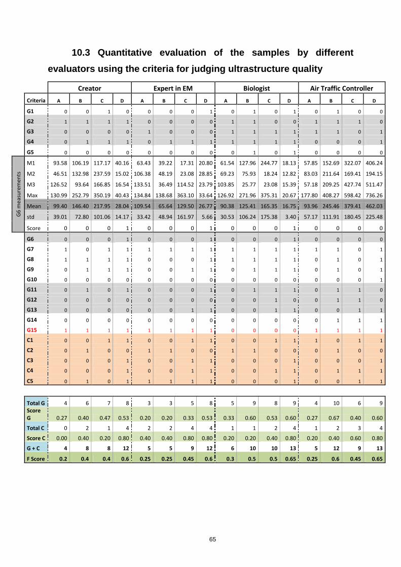
65
10.3 Quantitative evaluation of the samples by different
evaluators using the criteria for judging ultrastructure quality
Creator Expert in EM Biologist Air Traffic Controller
Criteria A B C D A B C D A B C D A B C D
G1 0 0 1 0 0 0 0 1 0 1 0 1 0 1 0 0
G2 1 1 1 1 0 0 0 0 1 1 0 0 1 1 1 0
G3 0 0 0 0 1 0 0 0 1 1 1 1 1 1 0 1
G4 0 1 1 1 0 1 1 1 1 1 1 1 0 0 0 1
G5 0 0 0 0 0 0 0 0 0 1 0 1 0 0 0 0
G6
mea
sure
men
ts
M1 93.58 106.19 117.17 40.16 63.43 39.22 17.31 20.80 61.54 127.96 244.77 18.13 57.85 152.69 322.07 406.24
M2 46.51 132.98 237.59 15.02 106.38 48.19 23.08 28.85 69.23 75.93 18.24 12.82 83.03 211.64 169.41 194.15
M3 126.52 93.64 166.85 16.54 133.51 36.49 114.52 23.79 103.85 25.77 23.08 15.39 57.18 209.25 427.74 511.47
Max 130.99 252.79 350.19 40.43 134.84 138.68 363.10 33.64 126.92 271.96 375.31 20.67 177.80 408.27 598.42 736.26
Mean 99.40 146.40 217.95 28.04 109.54 65.64 129.50 26.77 90.38 125.41 165.35 16.75 93.96 245.46 379.41 462.03
std 39.01 72.80 101.06 14.17 33.42 48.94 161.97 5.66 30.53 106.24 175.38 3.40 57.17 111.91 180.45 225.48
Score 0 0 0 1 0 0 0 1 0 0 0 1 0 0 0 0
G6 0 0 0 1 0 0 0 1 0 0 0 1 0 0 0 0
G7 1 0 1 1 1 1 1 1 1 1 1 1 1 1 0 1
G8 1 1 1 1 0 0 0 1 1 1 1 1 0 1 0 1
G9 0 1 1 1 0 0 1 1 0 1 1 1 0 1 0 1
G10 0 0 0 0 0 0 0 0 0 0 0 0 0 0 0 1
G11 0 1 0 1 0 0 0 1 0 1 1 1 0 1 1 0
G12 0 0 0 0 0 0 0 0 0 0 1 0 0 1 1 0
G13 0 0 0 0 0 0 1 1 0 0 1 1 0 0 1 1
G14 0 0 0 0 0 0 0 0 0 0 0 0 0 1 1 1
G15 1 1 1 1 1 1 1 1 0 0 0 0 1 1 1 1
C1 0 0 1 1 0 0 1 1 0 0 1 1 1 0 1 1
C2 0 1 0 0 1 1 0 0 1 1 0 0 0 1 0 0
C3 0 0 0 1 0 0 1 1 0 0 0 1 0 0 0 1
C4 0 0 0 1 0 0 1 1 0 0 1 1 0 1 1 1
C5 0 1 0 1 1 1 1 1 0 0 0 1 0 0 1 1
Total G 4 6 7 8 3 3 5 8 5 9 8 9 4 10 6 9
Score G 0.27 0.40 0.47 0.53 0.20 0.20 0.33 0.53 0.33 0.60 0.53 0.60 0.27 0.67 0.40 0.60
Total C 0 2 1 4 2 2 4 4 1 1 2 4 1 2 3 4
Score C 0.00 0.40 0.20 0.80 0.40 0.40 0.80 0.80 0.20 0.20 0.40 0.80 0.20 0.40 0.60 0.80
G + C 4 8 8 12 5 5 9 12 6 10 10 13 5 12 9 13
F Score 0.2 0.4 0.4 0.6 0.25 0.25 0.45 0.6 0.3 0.5 0.5 0.65 0.25 0.6 0.45 0.65
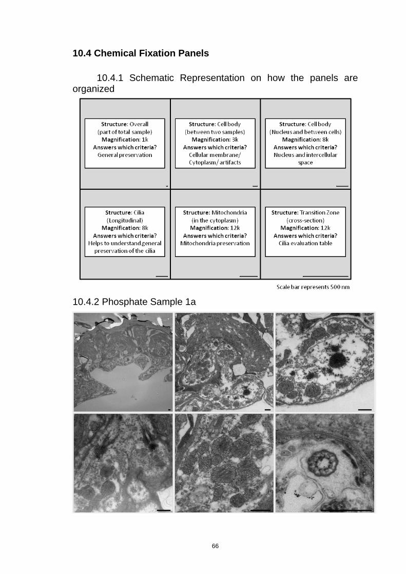
66
10.4 Chemical Fixation Panels
10.4.1 Schematic Representation on how the panels are organized
10.4.2 Phosphate Sample 1a

67
10.4.3 Phosphate Sample 1b
10.4.4 Phosphate Sample 1c

68
10.4.5 PHEM Sample 1a
10.4.6 PHEM Sample 1b

69
10.4.7 PHEM Sample 1c
10.4.8 Cacodylate Sample 1a

70
10.4.9 Cacodylate Sample 1b
10.4.10 Cacodylate Sample 1c
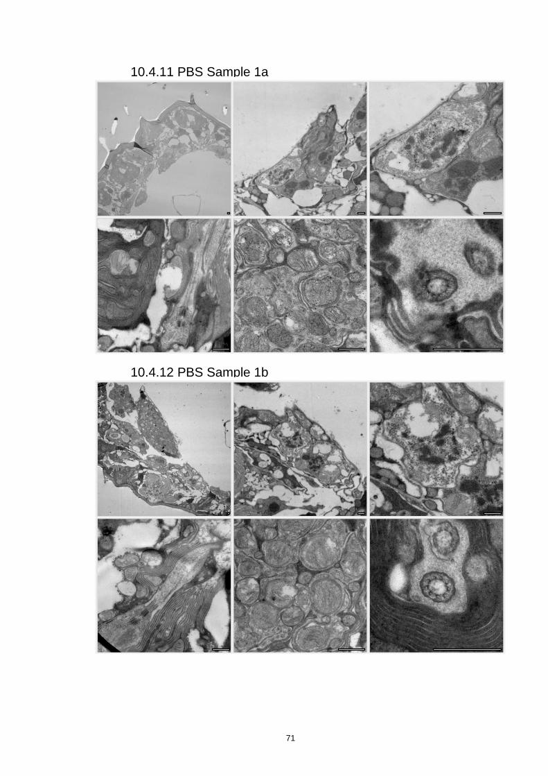
71
10.4.11 PBS Sample 1a
10.4.12 PBS Sample 1b
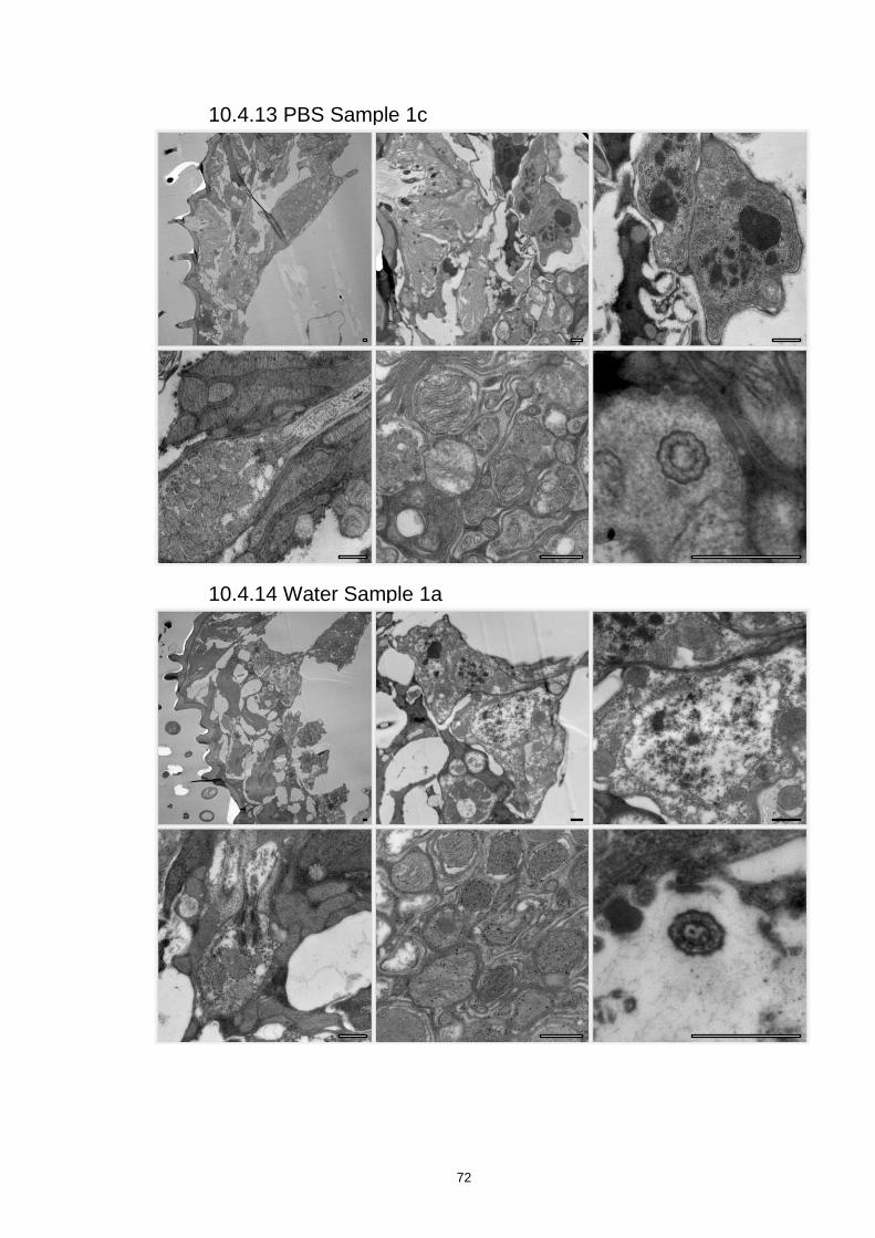
72
10.4.13 PBS Sample 1c
10.4.14 Water Sample 1a

73
10.4.15 Water Sample 1b
10.4.16 Water Sample 1c

74
10.4.17 Phosphate Sample 2
10.4.18 PHEM Sample 2

75
10.4.19 Cacodylate Sample 2
10.4.20 PBS Sample 2

76
10.4.21 Water Sample 2
10.4.22 Phosphate Sample 3

77
10.4.23 PHEM Sample 3
10.4.24 Cacodylate Sample 3

78
10.4.25 PBS Sample 3
10.4.26 Water Sample 3
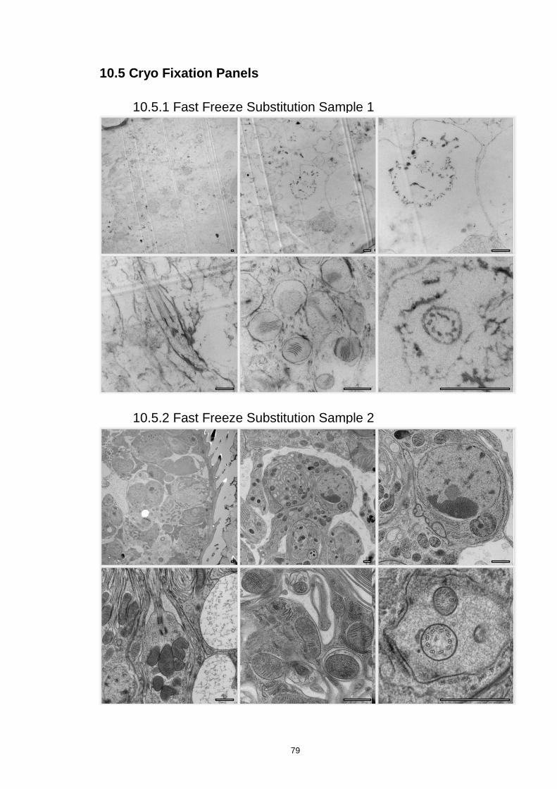
79
10.5 Cryo Fixation Panels
10.5.1 Fast Freeze Substitution Sample 1
10.5.2 Fast Freeze Substitution Sample 2

80
10.5.3 Medium Freeze Substitution Sample 1
10.5.4 Medium Freeze Substitution Sample 2
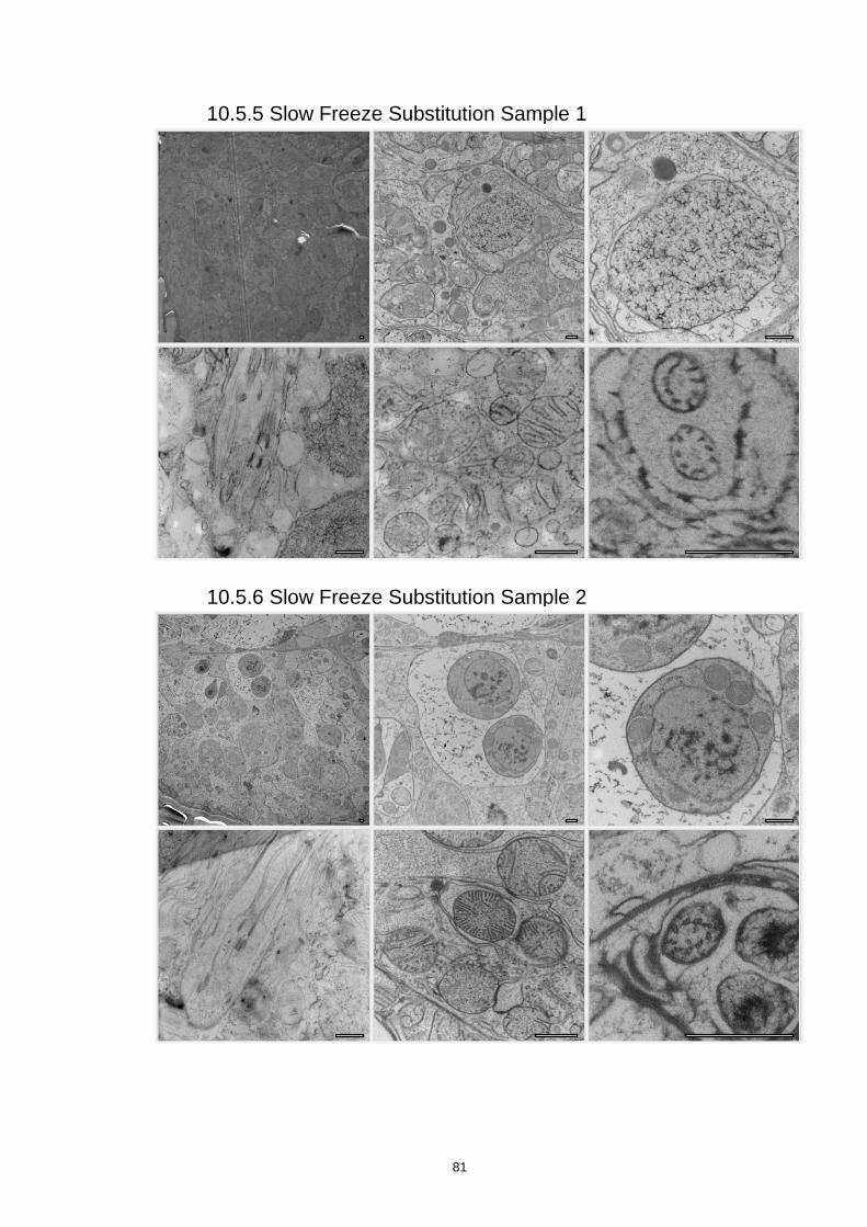
81
10.5.5 Slow Freeze Substitution Sample 1
10.5.6 Slow Freeze Substitution Sample 2

82
10.6 Materials, Reagents and Individual Protection Equipment
1-hexadecene, Merck, CAS# 629-73-2, Lot# S6852764
Acetone EM grade, Polysciences, CAS# 67-64-1, Lot# 648214
Bovine Serum Albumin, Sigma Aldrich, CAS# 9048-46-8, Lot# SLBH2718V
Centrifuge 5415D,ARS Plus, Eppendorf
Chloroform, Merck, CAS# 67-66-3, Lot# K45872845433
Cotton swabs
Dalmatian hair for section tips
DDSA, Electron Microscopy Sciences, CAS# 25377-73-5
Diamond Knife 45º, Diatome
Dibasic sodium phosphate, Calbiochem, CAS# 858-450-5558, Lot# D00140223
DMP-30, Electron Microscopy Sciences, CAS# 90-72-2
Drosophila melanogaster wild type, Bloomington
EGTA, Sigma Aldrich, CAS# 67-42-5, Lot# SLBB6797V
EMBed-812 Resin, Electron Microscopy Sciences, CAS# 25068-38-6
Eppendorfs, 1.5mL, Fisher Scientific
Ethanol Absolute, VWR Chemical, CAS# 64-17-5, Lot# 14G290521
Formaldehyde 16% ULTRA PURE Polysciences, Inc., CAS# 50-00-0, Lot# 647935
Formvar Powder, Agar scientific, CAS# 63148-64-1, Lot#R1201
Freeze substitution machine S6E, Leica
Gloves, Nitrile, Powder Free, Semper guard
Glutaraldehyde, EM grade 25% Polysciences, Inc., CAS 111-30-8, Lot# 667935
HEPES, Calbiochem, CAS# 858-450-5558, Lot# D00137935
High Pressure Freezing machine Compact 02, Engineering Office M. Wohlwend GmBH
Labcoat
Laboratory Glasswear
Lead Nitrate, Sigma Aldrich, CAS# 10099-74-8, Lot# BCBJ9164V
Liquid nitrogen recipients for transportation (custom made, designed by E. Tranfield)
Liquid nitrogen tank
Magnesium chloride hexahydrate (MgCl2.6H2O), Sigma Aldrich, CAS# 7791-18-6, Lot#
BCBF2018V
Methanol, VWR, CAS# 67-56-1, Lot# 14B210516
Molds for resin, Electron Microscopy Sciencies
Monobasic sodium Phosphate monohydrate, Sigma Aldrich, CAS# 7558-80-7, Lot#
021M00134V
Multiuse Labels 70x36mm, Staples
NMA, Electron Microscopy Sciences, CAS# 25134-21-8
Osmium tetroxide 0.1g, Electron Microscopy Sciences, CAS# 20816-12-0, Lot# 140708

83
Osmium tetroxide 1g, Electron Microscopy Sciences, CAS# 20816-12-0, Lot# 121011
Oven, Gentlab
Parafilm, roll 10cm wide, Reagente 5
PBS tablets, Sigma Aldrich, Product# P4417, Lot# 051M8213
pH meter Five Easy Plus, Mettler Toledo
PIPES, Sigma Aldrich, CAS# 5625-37-6, Lot# 110M54022V
Pipettes, Gilson
Propylene oxide, Sigma Aldrich, CAS# 75-56-9, Lot# 110205-1L
Razor blades, single edge extra keen, Electron Microscopy Sciences, Cat#71962
Rotator, Glas-Col
Scale Scout Pro 600g, DHAUS
Scissors
Slides Thermo Scientific Menzel-Glässer
Sodium Cacodylate Trihydrate, Sigma Aldrich, CAS# 6163-99-3, Lot# SLBF8273V
Sodium Citrate, Electron Microscopy Sciences, CAS# 6132-04-3, Lot# 080828
Sodium hydroxide pellets, Sigma Aldrich, CAS# 1310-73-2, Lot# BCBH5016V
Sodium tetraborate decahydrate, Fluka ANalytical, CAS# 1303-96-4, Lot# 1311713
Stereomicroscope SteREO Discovery. V8, ZEISS
Support for coating grids with Formvar (Custom made by UMC Utrecht, NL)
Syringe filters, Acrodisc 25mm w/ 0.2µm supor membrane, PALL, Lot#12463417
Syringe without needle, Terumo, Ref. SS+10ES1, Lot#140530W
Tags
Tape
Tips for pipettes
Toluidine Blue, Electron Microscopy Sciences, CAS# 92-31-9, Lot# 30113
Toothpicks
Transmission Electron Microscope model H-7650
Tungsten needle
Tweezers
Ultramicrotome Leica Reichert Ultracuts
Uranyl acetate, BDH chemicals Ltd, Product# 10288, Lot# 6437050
WFI (water for injection) quality water, Omnipur, Calbiochem, CAS# 7732-18-5, Lot#
98072062