prospects for consolidation Fiscal multipliers and - OECD. · PDF fileprospects for consolidation Ray Barrell, Dawn Holland, Ian Hurst Please cite this article as: Barrell ... differ

From:OECD Journal: Economic Studies

Access the journal at:http://dx.doi.org/10.1787/19952856

Fiscal multipliers andprospects for consolidation

Ray Barrell, Dawn Holland, Ian Hurst

Please cite this article as:

Barrell, Ray , Dawn Holland and Ian Hurst (2012), “Fiscal multipliersand prospects for consolidation”, OECD Journal: Economic Studies,Vol. 2012/1.http://dx.doi.org/10.1787/eco_studies-2012-5k8x6k5wc58x

http://dx.doi.org/10.1787/19952856

http://dx.doi.org/10.1787/eco_studies-2012-5k8x6k5wc58x

This document and any map included herein are without prejudice to the status of orsovereignty over any territory, to the delimitation of international frontiers and boundaries and tothe name of any territory, city or area.

OECD Journal: Economic Studies

Volume 2012

© OECD 2013

71

Fiscal multipliers and prospectsfor consolidation

by

Ray Barrell, Dawn Holland and Ian Hurst*

* Ray Barrell ([email protected]), Dawn Holland ([email protected]) and Ian Hurst([email protected]).The foundation of this paper is drawn from OECD Economics Department WorkingPaper No. 933. The authors wish to thank Jean-Luc Schneider, Peter Hoeller and Douglas Sutherland forhelpful comments on earlier drafts and are indebted to Sveinbjörn Blöndal and Anne Épaulard forcomments and suggestions. The views expressed in this article are those of the authors and do notnecessarily reflect those of the OECD or the governments of its member countries.

This article looks at various aspects of fiscal consolidation in 18 OECD economies.The prospects for fiscal consolidation depend upon the problems a country may facewith its debt stock, the political will to deal with these problems and on the costs ofconsolidation. These costs are a function of the impacts of fiscal policy on theeconomy, which is the focus of this study. The analysis is based on a series ofsimulations using the National Institute Global Econometric Model, NiGEM. Fiscalmultipliers differ across countries because the structure and behaviour of economiesdiffer. They also differ within countries, depending on factors such as the fiscalinstrument implemented, the policy response to fiscal innovations, and expectationformation by economic agents. The purpose of this study is to allow an assessmentof the likely impact on the economy and on the fiscal position of consolidationprogrammes. We decompose the key factors that determine the size of the multiplierby changing them one at a time. Even under a specified set of assumptions, theoutturn for the budget balance retains a high degree of uncertainty. We illustratethis uncertainty by calibrating probability bounds around projected debt profiles.This can allow an assessment of the probability of achieving specified fiscal targets,such as those set out in the European Union’s new Fiscal Compact.

JEL classification codes: E17; E37; E62

Key words: Large scale structural macro models; fiscal multipliers; rationalexpectations; budget consolidation in the OECD

FISCAL MULTIPLIERS AND PROSPECTS FOR CONSOLIDATION

OECD JOURNAL: ECONOMIC STUDIES – VOLUME 2012 © OECD 201372

The severe recessions as a result of the financial crisis in 2008-09 resulted in a sharp rise in

government budget deficits in almost all major industrialised countries. The cyclical impact

was compounded by fiscal stimulus packages and emergency financial sector support. This

in turn has led to a sharp rise in global government debt, giving rise to concerns about long-

term fiscal sustainability. Pressures have been particularly high in some euro area countries,

which have pushed government bond yields to exceptionally high levels in some countries

such as Spain, Italy, Portugal and Greece. As a result, fiscal consolidation packages have been

introduced by many of the major economies to stem the rise in sovereign debt.

This paper considers the impacts of fiscal consolidation on GDP growth in 18 OECD

economies. The analysis is based on a series of simulations using the National Institute

Global Econometric Model, NiGEM.1 The key features of the model are that it is estimated and

has a common structure across the 18 countries. If the results differ across countries it will

be because they are different. Some of these differences, such as the openness of the

economy, are important. They change over time and they are not related to estimation.

Others, such as the speed of response to changes in income, do depend upon how the model

was estimated. Details underlying key equations and the core structure of NiGEM are given

in the Appendix.

Fiscal multipliers differ across countries because the structure and behaviour of

economies differ. They also differ within countries, depending on factors such as the fiscal

instrument implemented, the policy response to fiscal innovations, and expectation

formation by economic agents. Much of the recent literature on fiscal multipliers also

suggests that the size of the multiplier may also depend on the state of the economy (see, for

example, Delong and Summers, 2012; Auerbach and Gorodnichenko, 2012). Others have

focused on identifying links between the fiscal position and the risk premium on government

borrowing, which is of particular importance in the euro area (see e.g. Arghyrou and

Kontonikas, 2011; Bernoth et al., 2012; De Grauwe and Ji, 2012; Schuknect et al., 2010, Corsetti

et al., 2012).

The purpose of this study is to allow an assessment of the likely impact on the economy

and on the fiscal position of the consolidation programmes that are being introduced. The

impact will depend on the factors discussed above – structure and behaviour of the economy,

fiscal instruments, expectation formation, policy response, state of the economy – and we

decompose these factors by changing them one at a time. Even under a specified set of

assumptions, the outturn for the budget balance retains a high degree of uncertainty. We

illustrate this uncertainty in selected countries by calibrating probability bounds around the

projected debt profiles.This can allow an assessment of the probability of achieving specified

fiscal targets, such as those set out in the European Union’s new Fiscal Compact.

1. Short-term impact multipliersBarrell, Fic and Liadze (2009) demonstrate that multipliers are time and state dependent.

Fiscal multipliers differ across countries because the structure and behaviour of economies


OECD JOURNAL: ECONOMIC STUDIES – VOLUME 2012 © OECD 2013 73

differ. They also differ within countries, depending on factors such as the fiscal instrument

implemented, the policy response to fiscal innovations, and expectation formation by

economic agents.Thus there is no single “multiplier” that can be attributed to a given economy,

as the impact of a fiscal innovation on GDP depends on a wide range of factors. In this section

we decompose the impact of several of these factors by changing them one at a time.

1.1. Fiscal instruments

In a model such as NiGEM multipliers are small. They average around 0.3 or less, as can

be seen from Tables 1 and 4 below. Even then these estimates probably exceed the

multipliers that one would see with any actual consolidation programme, because for some

actions implementation speed is faster in the model than in the world. If one allows for more

gradual implementation, this would reduce average multipliers to below 0.2. This matters in

particular when comparing multipliers for taxes and benefits to those for spending. Taxes or

benefits can be cut by 1% of GDP relatively easily both in the model and in the world.

Multipliers in response to income tax and benefit adjustments are small, as a part of the

decline in personal sector income is offset by a temporary adjustment in the savings rate. As

one can see from the tables, multipliers appear larger for cuts in real government spending.

This is in part because of the assumption that such cuts can be implemented immediately,

and this is certainly not the case. It is also in part because government consumption is part

of the income identity and hence when it is cut (and the number of people employed or goods

and services bought is reduced) measured real output falls. If one were to reduce government

spending by as much, but do it through wage reductions, then the impact on real GDP would

be much less, and the second round effects of the shock would effectively be the same as an

increase in taxes.

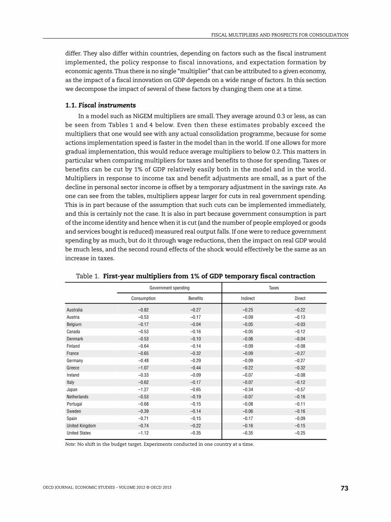
Table 1. First-year multipliers from 1% of GDP temporary fiscal contraction

Government spending Taxes

Consumption Benefits Indirect Direct

Australia –0.82 –0.27 –0.25 –0.22

Austria –0.53 –0.17 –0.09 –0.13

Belgium –0.17 –0.04 –0.05 –0.03

Canada –0.53 –0.16 –0.05 –0.12

Denmark –0.53 –0.10 –0.06 –0.04

Finland –0.64 –0.14 –0.09 –0.08

France –0.65 –0.32 –0.09 –0.27

Germany –0.48 –0.29 –0.09 –0.27

Greece –1.07 –0.44 –0.22 –0.32

Ireland –0.33 –0.09 –0.07 –0.08

Italy –0.62 –0.17 –0.07 –0.12

Japan –1.27 –0.65 –0.34 –0.57

Netherlands –0.53 –0.19 –0.07 –0.16

Portugal –0.68 –0.15 –0.08 –0.11

Sweden –0.39 –0.14 –0.06 –0.16

Spain –0.71 –0.15 –0.17 –0.09

United Kingdom –0.74 –0.22 –0.16 –0.15

United States –1.12 –0.35 –0.35 –0.25

Note: No shift in the budget target. Experiments conducted in one country at a time.



In order to determine the effects of an ex ante change in fiscal policy one has to avoid

offsetting or reinforcing policy effects, but the model must otherwise be allowed to run. In

each of our simulations in this section we make the following assumptions:

● Policy reactions are turned off for the first year:

❖ The central bank does not change the short-term interest rate for a year, whatever the

shock. It then follows a targeting regime that stabilises either the inflation rate or the

price level.

❖ The government does not target the deficit for the first year. The model has a feedback

rule which adjusts the direct tax rate in relation to the gap between actual and target

deficits. This is switched off for a year.

❖ Government investment is fixed at the baseline for a year and does not respond to long-

term factors in the first year. The same, where this is appropriate, is true for

government consumption.

❖ Other tax rates and all benefit replacement rates are held constant throughout the

simulation period.

● Markets work and all quantities and prices can react and there are no exogenous

variables in the model, with the exceptions of policy targets, labour supply and risk

premia:

❖ Financial markets look forward and are assumed to follow arbitrage paths, and

expectations for those paths are outturn consistent.

– Long-term government bond rates are the forward convolution of future short-term

policy rates plus an exogenous premium.

– Long-term real interest rates are the forward convolution of future short-term real

policy rates plus an exogenous risk premium made up of the bond premium plus

private sector risks.

– Equity prices are the discounted value of future profits, where the discount factor is

the market interest rate plus the exogenous equity premium.

– Exchange rates “jump” when future interest rates change and they follow the

arbitrage path given by nominal interest rates.

❖ Labour markets are described by an exogenous labour supply, a labour demand

equation and by a wage equation based on search theory, where the bargain depends

on backward and forward looking inflation expectations.

❖ Capital stocks adjust slowly towards that associated with expected capacity output four

years ahead, which in turn depends upon a forward looking user cost of capital.

Expectations are rational and factor demands and capacity output are based on a CES

production function.

❖ Consumers respond to their forward looking financial wealth, but are not fully forward

looking.

In the next sections, the implications of several of these default assumptions will be tested.

Table 1 reports the estimates of the first year multipliers for 18 OECD countries, under

the default assumptions described above, for a 1% (ex ante) GDP fiscal contraction – a rise in

taxes or cut in spending that is reversed after one year. The multipliers for cuts in

government consumption spending and spending on benefits are reported, as well as for

rises in indirect taxes and direct (personal) taxes. Simulations are run one country at a time,



so there are no spillovers across countries in the reported multipliers. Generally multipliers

peak in the first year and then decline, and the ex post improvement in government revenues

will normally be less than 1% of GDP as tax bases change. Some of the effects of the impulse

will be offset by declines in interest rates. Both short and long rates should fall, but the former

may be trapped at the lower bound at present. Even when short rates are trapped at the lower

bound, forward-looking long rates can fall as long as they retain some downward flexibility.

In NiGEM, investment behaviour is mainly influenced by long real rates through the user cost

of capital, and as long as these are free to fall in response to a temporary fiscal tightening, the

impact of hitting the zero bound in short rates will be limited.

The multipliers reported in Table 1 illustrate some of the key differences across fiscal

instruments, and also highlight important differences across countries. Government

consumption spending multipliers tend to be larger than tax or benefit multipliers, as a

fraction of any disposable income change is absorbed through a temporary adjustment to

savings. However we should bear in mind the caveat mentioned above that it is not necessarily

feasible to cut the provision of government goods and services at short notice. The effects of

government investment and corporate taxes will not be investigated in this study.2

1.2. Structure of the economy

Country size is an important distinguishing factor across country multipliers, as the long

term fall in real interest rates that is produced by consolidations is an international

phenomenon. When capital moves freely between countries, real interest rates are

determined largely by the balance between global saving and global investment, and large

countries such as the United States have much more impact than small ones such as Greece.

In addition, the initial interest rate response will be smaller in countries in EMU because the

ECB responds to euro area inflation.

Multipliers tend to be smaller in more open economies, because the more open an

economy is the more of a shock will spread into other countries through imports, and small

open economies such as Belgium have small multipliers. Another structuring factor is the

degree of dependence of consumption on current income. This is often related to liquidity

constraints, with a higher current-income elasticity more common in financially unliberalised

economies such as Greece than in Belgium or the United States. Finally, the speed of

response of the economy depends in part on the flexibility of the labour market and the

speed at which policies, such as a rise in VAT feed into prices.

Table 2 compares the temporary government consumption spending and direct tax

multipliers from Table 1 with some of the key factors determining the differences in the

magnitude of multipliers across countries: country size (measured at 2005 PPPs), import

penetration (measured as the volume of imports of goods and services in 2005 as a share of

GDP) and the estimated short-term income elasticity of consumption. At the bottom of the

table, the correlations between each factor and the two multipliers are reported. The largest

estimated multipliers are found in Japan, the United States and Greece. For Japan and the

United States this is largely a reflection of the low level of import leakages, with imports

amounting to just 10-15% of GDP. Import penetration is also relatively low in Greece, given

the size of the economy, while the estimated short-term income elasticity of consumption is

higher than in most of the other economies in the sample, and both factors increase the

estimated multiplier.



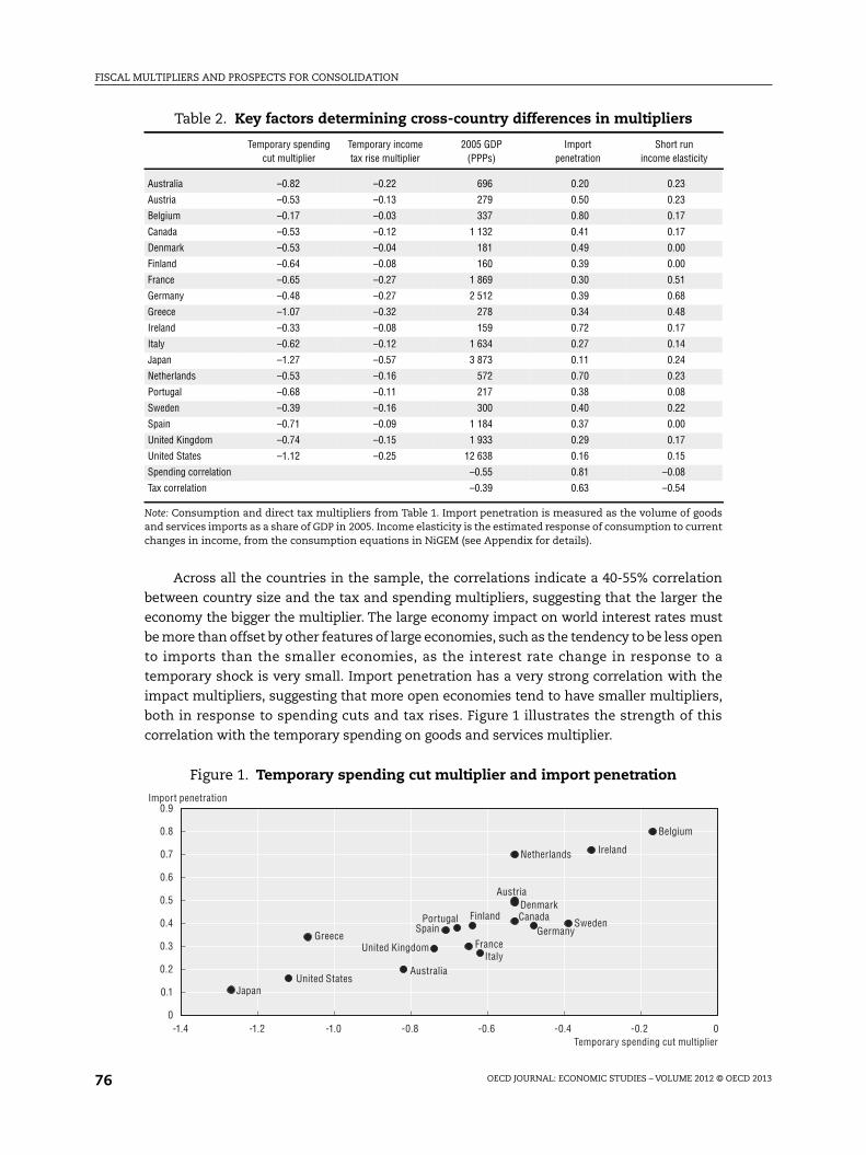
Across all the countries in the sample, the correlations indicate a 40-55% correlation

between country size and the tax and spending multipliers, suggesting that the larger the

economy the bigger the multiplier. The large economy impact on world interest rates must

be more than offset by other features of large economies, such as the tendency to be less open

to imports than the smaller economies, as the interest rate change in response to a

temporary shock is very small. Import penetration has a very strong correlation with the

impact multipliers, suggesting that more open economies tend to have smaller multipliers,

both in response to spending cuts and tax rises. Figure 1 illustrates the strength of this

correlation with the temporary spending on goods and services multiplier.

Table 2. Key factors determining cross-country differences in multipliers

Temporary spendingcut multiplier

Temporary incometax rise multiplier

2005 GDP(PPPs)

Importpenetration

Short runincome elasticity

Australia –0.82 –0.22 696 0.20 0.23

Austria –0.53 –0.13 279 0.50 0.23

Belgium –0.17 –0.03 337 0.80 0.17

Canada –0.53 –0.12 1 132 0.41 0.17

Denmark –0.53 –0.04 181 0.49 0.00

Finland –0.64 –0.08 160 0.39 0.00

France –0.65 –0.27 1 869 0.30 0.51

Germany –0.48 –0.27 2 512 0.39 0.68

Greece –1.07 –0.32 278 0.34 0.48

Ireland –0.33 –0.08 159 0.72 0.17

Italy –0.62 –0.12 1 634 0.27 0.14

Japan –1.27 –0.57 3 873 0.11 0.24

Netherlands –0.53 –0.16 572 0.70 0.23

Portugal –0.68 –0.11 217 0.38 0.08

Sweden –0.39 –0.16 300 0.40 0.22

Spain –0.71 –0.09 1 184 0.37 0.00

United Kingdom –0.74 –0.15 1 933 0.29 0.17

United States –1.12 –0.25 12 638 0.16 0.15

Spending correlation –0.55 0.81 –0.08

Tax correlation –0.39 0.63 –0.54

Note: Consumption and direct tax multipliers from Table 1. Import penetration is measured as the volume of goodsand services imports as a share of GDP in 2005. Income elasticity is the estimated response of consumption to currentchanges in income, from the consumption equations in NiGEM (see Appendix for details).

Figure 1. Temporary spending cut multiplier and import penetration

0.9

0.8

0.7

0.6

0.5

0.4

0.3

0.2

0.1

0-1.2-1.4 -0.8-1.0 -0.4-0.6 0-0.2

Temporary spending cut multiplier

Import penetration

Belgium

CanadaDenmark

Finland

FranceGermanyGreece

United StatesAustralia

United Kingdom

Ireland

Italy

Japan

Netherlands

Austria

Portugal SwedenSpain



The short-term income elasticity of consumption has little relationship with the first

year government consumption multipliers, as government consumption is a direct

component of GDP, and the impacts on GDP via the household consumption channel are

secondary. However, this elasticity shows a 50% correlation with income tax multipliers,

which feed directly into personal income, and affect GDP through the household

consumption channel. The indirect tax and benefit multipliers will also depend upon the

short-term relationship between income and consumption. An indirect tax increase reduces

real income, and the extent to which this feeds into GDP is directly related to the short-term

income elasticity of consumption. Similarly, benefit payments are a component of income,

and affect GDP through the consumption channel, so first-year multipliers for these

instruments will also be sensitive to the short-term income elasticity of consumption.

Fiscal multipliers are clearly sensitive to the short-term income elasticity of consumption,

which is commonly associated with the severity of borrowing constraints within the

economy. However, access to credit is dependent both on credit history and on current

income, and so is necessarily sensitive to the state of the economy. As unemployment rises,

a greater share of the population will be unable to access credit at reasonable rates of interest

– at precisely the moment when they are in need of borrowing to smooth their consumption

path. This means that consumption is likely to be cyclical, and that the income elasticity is

likely to be time varying and dependent on the position in the cycle. Following a banking

crisis the effects can be expected to be particularly acute, as banks tighten lending criteria,

as discussed by Barrell, Fic and Liadze (2009). This also suggests that fiscal multipliers are

dependent on the state of the economy – especially tax innovation multipliers – and this is

consistent with recent studies such as Delong and Summers (2012) and Auerbach and

Gorodnichenko (2012).

The consumption equations3 underlying the multiplier estimates reported in Table 1 are

modelled as:

(1)

where C is consumption, TAW is total asset wealth, which is the sum of net financial wealth

(NW) and tangible wealth (HW), RPDI is real personal disposable income, is the difference

operator, and the remaining symbols are parameters. The share of the population that is

liquidity constrained will affect the short-term income elasticity of consumption, given by

parameter b1. Al Eyd and Barrell (2005) discuss this further.

In order to assess the sensitivity of fiscal multipliers to this parameter, we calibrate the

income tax multiplier under a series of eleven different models, allowing the parameter b1 to

rise incrementally. We illustrate the sensitivity using the United States as an example.

When b1 is equal to 0, this implies perfect capital markets with no liquidity constraints and

consumer spending will be largely invariant to short-term fluctuations in income. When it is

equal to 1 this implies that consumption is fully reliant on current income, with no scope for

saving and smoothing consumption. In our standard model, the estimated parameter for b1

in the United States is given by 0.15, suggesting a relatively low level of liquidity constraints

historically, although as Table 2 illustrates this is not out of line with other advanced

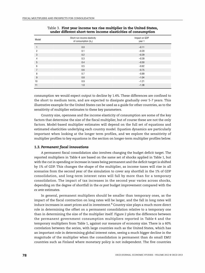
economies in an internationally comparative context. The estimated fiscal multipliers of

income tax innovations under different assumptions on the short-run income elasticity of

consumption are reported in Table 3. With no liquidity constraints, we would expect a fiscal

multiplier of just 0.1% in the first year, while with no options for borrowing to smooth

� � � � � � � � � �� ttt

tttt

HWbNWbRPDIbRPDIbTAWbaCC

lnlnlnln1lnlnln

321

10101

��



consumption we would expect output to decline by 1.4%. These differences are confined to

the short to medium term, and are expected to dissipate gradually over 5-7 years. This

illustrative example for the United States can be used as a guide for other countries, as to the

sensitivity of multiplier estimates to these key parameters.

Country size, openness and the income elasticity of consumption are some of the key

factors that determine the size of the fiscal multiplier, but of course these are not the only

factors. Model-based multiplier estimates will depend on the full set of equations and

estimated elasticities underlying each country model. Equation dynamics are particularly

important when looking at the longer term profiles, and we explore the sensitivity of

multiplier profiles to key equations in the section on longer-term multiplier profiles below.

1.3. Permanent fiscal innovations

A permanent fiscal consolidation also involves changing the budget deficit target. The

reported multipliers in Table 4 are based on the same set of shocks applied in Table 1, but

with the cut in spending or increase in taxes being permanent and the deficit target is shifted

by 1% of GDP. This changes the shape of the multiplier, as income taxes will rise in all

scenarios from the second year of the simulation to cover any shortfall in the 1% of GDP

consolidation, and long-term interest rates will fall by more than for a temporary

consolidation. The impact of tax increases in the second year varies across shocks,

depending on the degree of shortfall in the ex post budget improvement compared with the

ex ante estimates.

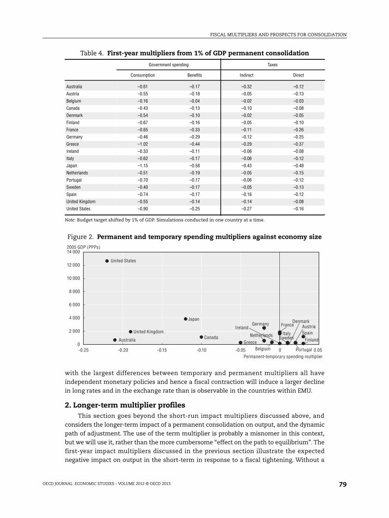
In general, permanent multipliers should be smaller than temporary ones, as the

impact of the fiscal contraction on long rates will be larger, and the fall in long rates will

induce increases in asset prices and in investment.4 Country size plays a much more direct

role in determining the offset on a permanent consolidation relative to a temporary one

than in determining the size of the multiplier itself. Figure 2 plots the difference between

the permanent government consumption multipliers reported in Table 4 and the

temporary multipliers from Table 1, against our measure of economy size. There is a 60%

correlation between the series, with large countries such as the United States, which has

an important role in determining global interest rates, seeing a much bigger decline in the

magnitude of the multiplier when the consolidation is permanent than do small EMU

countries such as Finland where monetary policy is not independent. The five countries

Table 3. First year income tax rise multiplier in the United States,under different short-term income elasticities of consumption

ModelShort-run income elasticity

of consumption (b1)Impact on GDP

year 1

1 0.0 –0.11

2 0.1 –0.20

3 0.2 –0.29

4 0.3 –0.39

5 0.4 –0.50

6 0.5 –0.62

7 0.6 –0.75

8 0.7 –0.89

9 0.8 –1.04

10 0.9 –1.21

11 1.0 –1.38



with the largest differences between temporary and permanent multipliers all have

independent monetary policies and hence a fiscal contraction will induce a larger decline

in long rates and in the exchange rate than is observable in the countries within EMU.

2. Longer-term multiplier profilesThis section goes beyond the short-run impact multipliers discussed above, and

considers the longer-term impact of a permanent consolidation on output, and the dynamic

path of adjustment. The use of the term multiplier is probably a misnomer in this context,

but we will use it, rather than the more cumbersome “effect on the path to equilibrium”. The

first-year impact multipliers discussed in the previous section illustrate the expected

negative impact on output in the short-term in response to a fiscal tightening. Without a

Table 4. First-year multipliers from 1% of GDP permanent consolidation

Government spending Taxes

Consumption Benefits Indirect Direct

Australia –0.61 –0.17 –0.32 –0.12

Austria –0.55 –0.18 –0.05 –0.13

Belgium –0.16 –0.04 –0.02 –0.03

Canada –0.43 –0.13 –0.10 –0.08

Denmark –0.54 –0.10 –0.02 –0.05

Finland –0.67 –0.16 –0.05 –0.10

France –0.65 –0.33 –0.11 –0.26

Germany –0.46 –0.29 –0.12 –0.25

Greece –1.02 –0.44 –0.29 –0.37

Ireland –0.33 –0.11 –0.06 –0.08

Italy –0.62 –0.17 –0.06 –0.12

Japan –1.15 –0.58 –0.43 –0.48

Netherlands –0.51 –0.19 –0.05 –0.15

Portugal –0.70 –0.17 –0.06 –0.12

Sweden –0.40 –0.17 –0.05 –0.13

Spain –0.74 –0.17 –0.16 –0.12

United Kingdom –0.55 –0.14 –0.14 –0.08

United States –0.90 –0.25 –0.27 –0.16

Note: Budget target shifted by 1% of GDP. Simulations conducted in one country at a time.

Figure 2. Permanent and temporary spending multipliers against economy size

14 000

12 000

10 000

8 000

6 000

4 000

2 000

0-0.25 -0.20 -0.15 -0.10 -0.05 0 0.05

2005 GDP (PPPs)

Permanent-temporary spending multiplier

Canada

FranceGermanyIreland

Italy

Japan

United Kingdom

United States

AustraliaNetherlands

Belgium

Finland

Portugal

GreeceSweden

Denmark

SpainAustria



simultaneous shock to the supply side of the economy, the demand shock will dissipate over

time, bringing the level of output back towards its long-run equilibrium. The transmission

mechanisms that allow output to recover are primarily through the financial markets and

price adjustment. The contraction in demand leads to job losses and puts downward

pressure on the price level. Higher unemployment leads to more moderate wage settlements,

strengthening the disinflationary pressures. This allows interest rates to come down and a

depreciation of the exchange rate, which in turn stimulate investment and net trade. While

there will be a shift in the composition of demand (from the public to the private sector, or

from consumption to investment and net trade) the level of output should return to base. In

general, in large economies output should rise marginally in the long run in response to a

fiscal consolidation in that country alone, as real interest rates will eventually be lower. This

raises the desired level of the capital stock and thus potential output over the longer term.

The profiles for a number of countries are reported, and each starts with the impact

multipliers in Table 4.

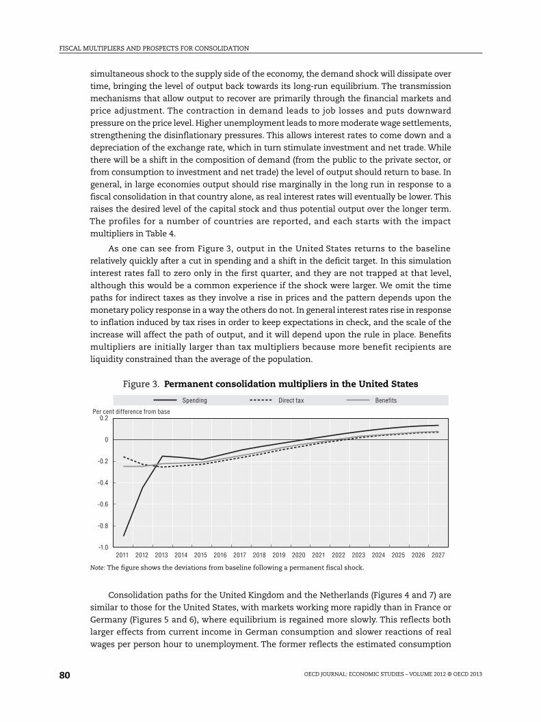
As one can see from Figure 3, output in the United States returns to the baseline

relatively quickly after a cut in spending and a shift in the deficit target. In this simulation

interest rates fall to zero only in the first quarter, and they are not trapped at that level,

although this would be a common experience if the shock were larger. We omit the time

paths for indirect taxes as they involve a rise in prices and the pattern depends upon the

monetary policy response in a way the others do not. In general interest rates rise in response

to inflation induced by tax rises in order to keep expectations in check, and the scale of the

increase will affect the path of output, and it will depend upon the rule in place. Benefits

multipliers are initially larger than tax multipliers because more benefit recipients are

liquidity constrained than the average of the population.

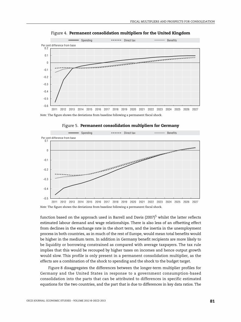
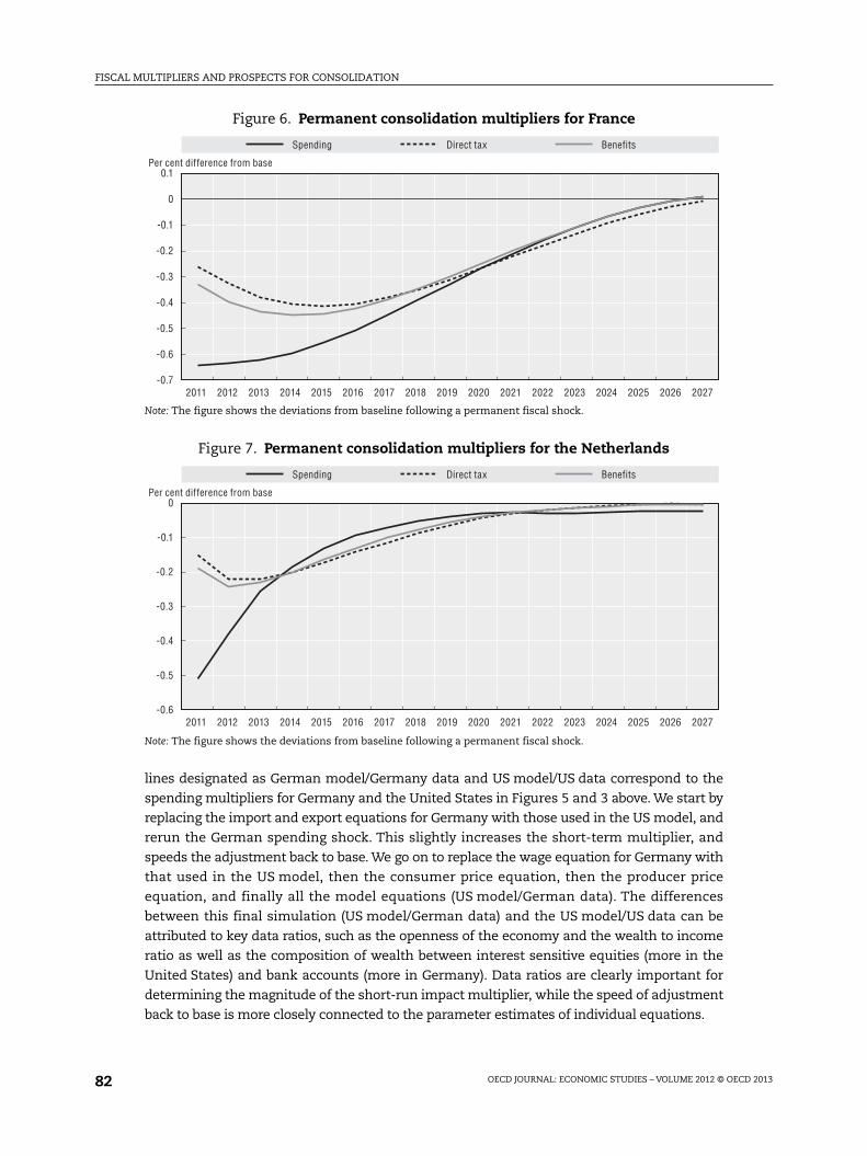
Consolidation paths for the United Kingdom and the Netherlands (Figures 4 and 7) are

similar to those for the United States, with markets working more rapidly than in France or

Germany (Figures 5 and 6), where equilibrium is regained more slowly. This reflects both

larger effects from current income in German consumption and slower reactions of real

wages per person hour to unemployment. The former reflects the estimated consumption

Figure 3. Permanent consolidation multipliers in the United States

Note: The figure shows the deviations from baseline following a permanent fiscal shock.

0.2

0

-0.2

-0.4

-0.6

-0.8

-1.02011 2012 2013 2014 2015 2016 2017 2018 2019 2020 2021 2022 2023 2024 2025 2026 2027

Spending Direct tax Benefits

Per cent difference from base



function based on the approach used in Barrell and Davis (2007)5 whilst the latter reflects

estimated labour demand and wage relationships. There is also less of an offsetting effect

from declines in the exchange rate in the short term, and the inertia in the unemployment

process in both countries, as in much of the rest of Europe, would mean total benefits would

be higher in the medium term. In addition in Germany benefit recipients are more likely to

be liquidity or borrowing constrained as compared with average taxpayers. The tax rule

implies that this would be recouped by higher taxes on incomes and hence output growth

would slow. This profile is only present in a permanent consolidation multiplier, as the

effects are a combination of the shock to spending and the shock to the budget target.

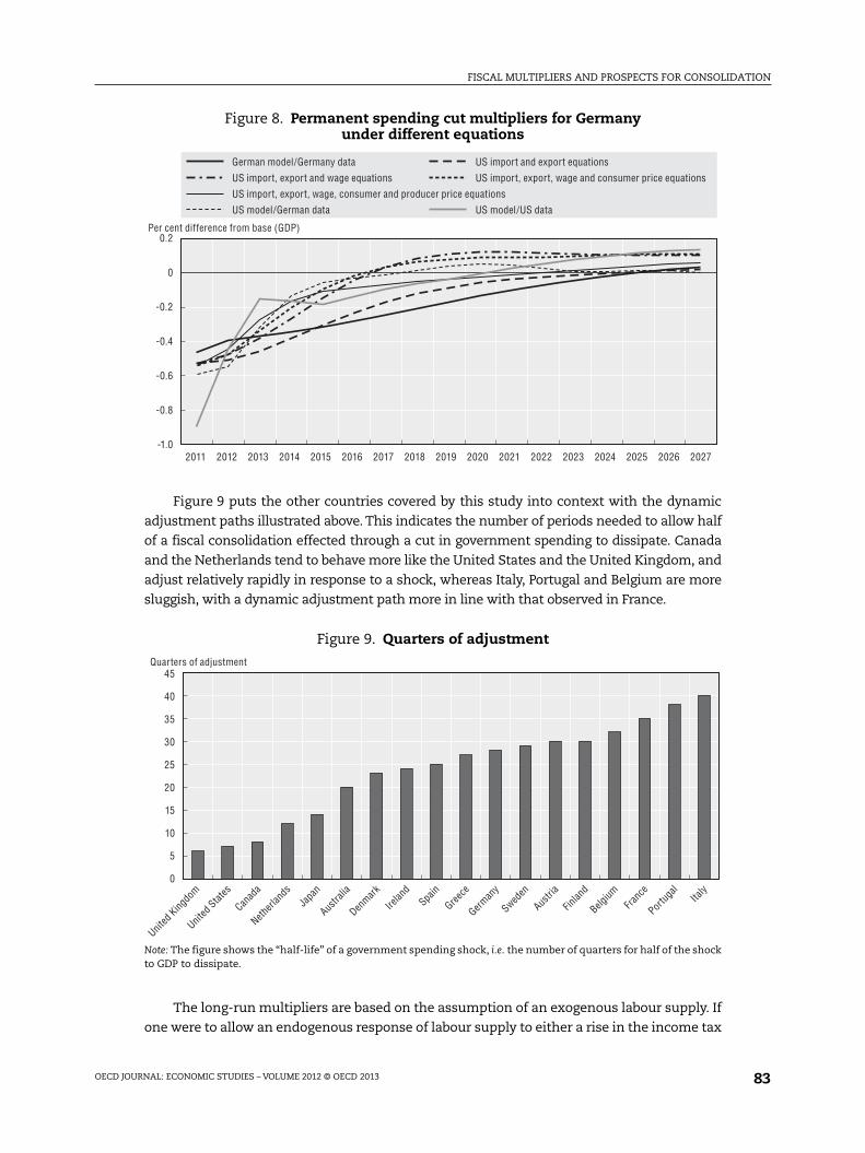
Figure 8 disaggregates the differences between the longer-term multiplier profiles for

Germany and the United States in response to a government consumption-based

consolidation into the parts that can be attributed to differences in specific estimated

equations for the two countries, and the part that is due to differences in key data ratios. The

Figure 4. Permanent consolidation multipliers for the United Kingdom


Figure 5. Permanent consolidation multipliers for Germany


0.2

0.1

0

-0.2

-0.1

-0.3

-0.4

-0.5

-0.62011 2012 2013 2014 2015 2016 2017 2018 2019 2020 2021 2022 2023 2024 2025 2026 2027



0.1

0

-0.1

-0.2

-0.3

-0.4

-0.52011 2012 2013 2014 2015 2016 2017 2018 2019 2020 2021 2022 2023 2024 2025 2026 2027





lines designated as German model/Germany data and US model/US data correspond to the

spending multipliers for Germany and the United States in Figures 5 and 3 above. We start by

replacing the import and export equations for Germany with those used in the US model, and

rerun the German spending shock. This slightly increases the short-term multiplier, and

speeds the adjustment back to base. We go on to replace the wage equation for Germany with

that used in the US model, then the consumer price equation, then the producer price

equation, and finally all the model equations (US model/German data). The differences

between this final simulation (US model/German data) and the US model/US data can be

attributed to key data ratios, such as the openness of the economy and the wealth to income

ratio as well as the composition of wealth between interest sensitive equities (more in the

United States) and bank accounts (more in Germany). Data ratios are clearly important for

determining the magnitude of the short-run impact multiplier, while the speed of adjustment

back to base is more closely connected to the parameter estimates of individual equations.

Figure 6. Permanent consolidation multipliers for France


Figure 7. Permanent consolidation multipliers for the Netherlands


0.1

0

-0.1

-0.2

-0.3

-0.4

-0.7

-0.5

-0.6

2011 2012 2013 2014 2015 2016 2017 2018 2019 2020 2021 2022 2023 2024 2025 2026 2027



0

-0.1

-0.2

-0.3

-0.4

-0.5

-0.62011 2012 2013 2014 2015 2016 2017 2018 2019 2020 2021 2022 2023 2024 2025 2026 2027





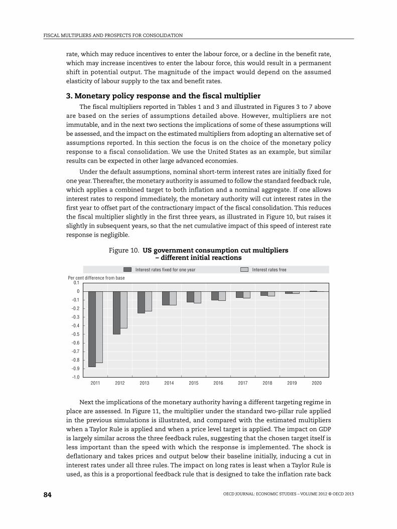
Figure 9 puts the other countries covered by this study into context with the dynamic

adjustment paths illustrated above. This indicates the number of periods needed to allow half

of a fiscal consolidation effected through a cut in government spending to dissipate. Canada

and the Netherlands tend to behave more like the United States and the United Kingdom, and

adjust relatively rapidly in response to a shock, whereas Italy, Portugal and Belgium are more

sluggish, with a dynamic adjustment path more in line with that observed in France.

The long-run multipliers are based on the assumption of an exogenous labour supply. If

one were to allow an endogenous response of labour supply to either a rise in the income tax

Figure 8. Permanent spending cut multipliers for Germanyunder different equations

Figure 9. Quarters of adjustment

Note: The figure shows the “half-life” of a government spending shock, i.e. the number of quarters for half of the shockto GDP to dissipate.

0.2

0

-0.2

-0.4

-0.6

-0.8

-1.02011 2012 2013 2014 2015 2016 2017 2018 2019 2020 2021 2022 2023 2024 2025 2026 2027

US model/US data

US import, export, wage, consumer and producer price equations

US model/German data

US import, export and wage equations US import, export, wage and consumer price equations

German model/Germany data US import and export equations

Per cent difference from base (GDP)

45

40

35

30

25

20

15

10

5

0

United

Kingdo

m

United

States

Canad

a

Netherl

ands

Japa

n

Austra

lia

Denmark

Irelan

dSpa

in

Greece

German

y

Sweden

Austri

a

Finlan

d

Belgium

Franc

e

Portug

alIta

ly

Quarters of adjustment



rate, which may reduce incentives to enter the labour force, or a decline in the benefit rate,

which may increase incentives to enter the labour force, this would result in a permanent

shift in potential output. The magnitude of the impact would depend on the assumed

elasticity of labour supply to the tax and benefit rates.

3. Monetary policy response and the fiscal multiplierThe fiscal multipliers reported in Tables 1 and 3 and illustrated in Figures 3 to 7 above

are based on the series of assumptions detailed above. However, multipliers are not

immutable, and in the next two sections the implications of some of these assumptions will

be assessed, and the impact on the estimated multipliers from adopting an alternative set of

assumptions reported. In this section the focus is on the choice of the monetary policy

response to a fiscal consolidation. We use the United States as an example, but similar

results can be expected in other large advanced economies.

Under the default assumptions, nominal short-term interest rates are initially fixed for

one year.Thereafter, the monetary authority is assumed to follow the standard feedback rule,

which applies a combined target to both inflation and a nominal aggregate. If one allows

interest rates to respond immediately, the monetary authority will cut interest rates in the

first year to offset part of the contractionary impact of the fiscal consolidation. This reduces

the fiscal multiplier slightly in the first three years, as illustrated in Figure 10, but raises it

slightly in subsequent years, so that the net cumulative impact of this speed of interest rate

response is negligible.

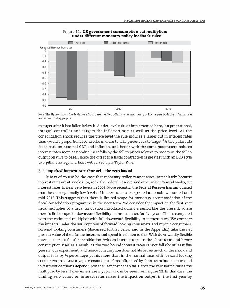
Next the implications of the monetary authority having a different targeting regime in

place are assessed. In Figure 11, the multiplier under the standard two-pillar rule applied

in the previous simulations is illustrated, and compared with the estimated multipliers

when a Taylor Rule is applied and when a price level target is applied. The impact on GDP

is largely similar across the three feedback rules, suggesting that the chosen target itself is

less important than the speed with which the response is implemented. The shock is

deflationary and takes prices and output below their baseline initially, inducing a cut in

interest rates under all three rules. The impact on long rates is least when a Taylor Rule is

used, as this is a proportional feedback rule that is designed to take the inflation rate back

Figure 10. US government consumption cut multipliers– different initial reactions

0.1

0

-0.1

-0.2

-0.3

-0.4

-0.5

-0.6

-0.7

-0.8

-0.9

-1.02011 2012 2013 2014 2015 2016 2017 2018 2019 2020

Interest rates fixed for one year Interest rates free




to target after it has fallen below it. A price level rule, as implemented here, is a proportional,

integral controller and targets the inflation rate as well as the price level. As the

consolidation shock reduces the price level the rule induces a larger cut in interest rates

than would a proportional controller in order to take prices back to target.6 A two pillar rule

feeds back on nominal GDP and inflation, and hence with the same parameters reduces

interest rates more as nominal GDP falls by the fall in prices relative to base plus the fall in

output relative to base. Hence the offset to a fiscal contraction is greatest with an ECB style

two pillar strategy and least with a Fed style Taylor Rule.

3.1. Impaired interest rate channel – the zero boundIt may of course be the case that monetary policy cannot react immediately because

interest rates are at, or close to, zero.The Federal Reserve, and other major Central Banks, cut

interest rates to near zero levels in 2009. More recently, the Federal Reserve has announced

that these exceptionally low levels of interest rates are expected to remain warranted until

mid-2015. This suggests that there is limited scope for monetary accommodation of the

fiscal consolidation programme in the near term. We consider the impact on the first-year

fiscal multiplier of a fiscal innovation introduced during a period like the present, where

there is little scope for downward flexibility in interest rates for five years. This is compared

with the estimated multiplier with full downward flexibility in interest rates. We compare

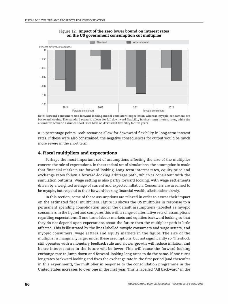
the impacts under the assumptions of forward looking consumers and myopic consumers.

Forward looking consumers (discussed further below and in the Appendix) take the net

present value of their future incomes and spend in relation to this. With downwardly flexible

interest rates, a fiscal consolidation reduces interest rates in the short term and hence

consumption rises as a result. At the zero bound interest rates cannot fall (for at least five

years in our experiment) and hence consumption does not absorb as much of the shock and

output falls by ¼ percentage points more than in the normal case with forward looking

consumers. In NiGEM myopic consumers are less influenced by short-term interest rates and

investment decisions depend upon the user cost of capital. Hence the zero bound raises the

multiplier by less if consumers are myopic, as can be seen from Figure 12. In this case, the

binding zero bound on interest rates raises the impact on output in the first year by

Figure 11. US government consumption cut multipliers– under different monetary policy feedback rules

Note: The figure shows the deviations from baseline. Two pillar is when monetary policy targets both the inflation rateand a nominal aggregate.

0

-0.1

-0.2

-0.3

-0.4

-0.5

-0.6

-0.8

-0.7

-0.9

-1.02011 2012 2013

Two pilar Price level target Taylor Rule




0.15 percentage points. Both scenarios allow for downward flexibility in long-term interest

rates. If these were also constrained, the negative consequences for output would be much

more severe in the short term.

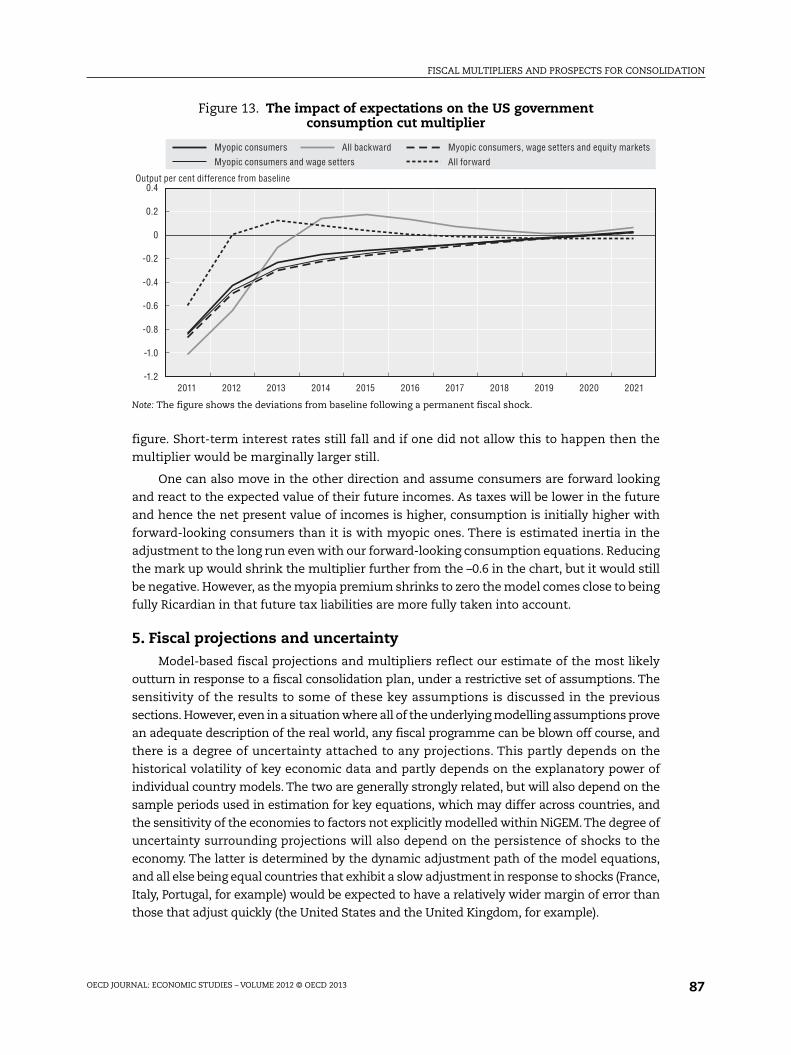
4. Fiscal multipliers and expectationsPerhaps the most important set of assumptions affecting the size of the multiplier

concern the role of expectations. In the standard set of simulations, the assumption is made

that financial markets are forward looking. Long-term interest rates, equity price and

exchange rates follow a forward-looking arbitrage path, which is consistent with the

simulation outturns. Wage setting is also partly forward looking, with wage settlements

driven by a weighted average of current and expected inflation. Consumers are assumed to

be myopic, but respond to their forward-looking financial wealth, albeit rather slowly.

In this section, some of these assumptions are relaxed in order to assess their impact

on the estimated fiscal multipliers. Figure 13 shows the US multiplier in response to a

permanent spending consolidation under the default assumptions (labelled as myopic

consumers in the figure) and compares this with a range of alternative sets of assumptions

regarding expectations. If one turns labour markets and equities backward looking so that

they do not depend upon expectations about the future then the multiplier path is little

affected. This is illustrated by the lines labelled myopic consumers and wage setters, and

myopic consumers, wage setters and equity markets in the figure. The size of the

multiplier is marginally larger under these assumptions, but not significantly so. The shock

still operates with a monetary feedback rule and slower growth will reduce inflation and

hence interest rates in the future will be lower. This will cause the forward-looking

exchange rate to jump down and forward-looking long rates to do the same. If one turns

long rates backward looking and fixes the exchange rate in the first period (and thereafter

in this experiment), the multiplier in response to the consolidation programme in the

United States increases to over one in the first year. This is labelled “All backward” in the

Figure 12. Impact of the zero lower bound on interest rateson the US government consumption cut multiplier

Note: Forward consumers use forward-looking model-consistent expectation whereas myopic consumers arebackward looking. The standard scenario allows for full downward flexibility in short-term interest rates, while thealternative scenario assumes short rates have no downward flexibility for five years.

0

-0.2

-0.4

-0.6

-0.8

-1.2

-1.0

2011 20112012 2012

Standard At zero bound


Forward consumers Myopic consumers



figure. Short-term interest rates still fall and if one did not allow this to happen then the

multiplier would be marginally larger still.

One can also move in the other direction and assume consumers are forward looking

and react to the expected value of their future incomes. As taxes will be lower in the future

and hence the net present value of incomes is higher, consumption is initially higher with

forward-looking consumers than it is with myopic ones. There is estimated inertia in the

adjustment to the long run even with our forward-looking consumption equations. Reducing

the mark up would shrink the multiplier further from the –0.6 in the chart, but it would still

be negative. However, as the myopia premium shrinks to zero the model comes close to being

fully Ricardian in that future tax liabilities are more fully taken into account.

5. Fiscal projections and uncertaintyModel-based fiscal projections and multipliers reflect our estimate of the most likely

outturn in response to a fiscal consolidation plan, under a restrictive set of assumptions. The

sensitivity of the results to some of these key assumptions is discussed in the previous

sections. However, even in a situation where all of the underlying modelling assumptions prove

an adequate description of the real world, any fiscal programme can be blown off course, and

there is a degree of uncertainty attached to any projections. This partly depends on the

historical volatility of key economic data and partly depends on the explanatory power of

individual country models. The two are generally strongly related, but will also depend on the

sample periods used in estimation for key equations, which may differ across countries, and

the sensitivity of the economies to factors not explicitly modelled within NiGEM.The degree of

uncertainty surrounding projections will also depend on the persistence of shocks to the

economy. The latter is determined by the dynamic adjustment path of the model equations,

and all else being equal countries that exhibit a slow adjustment in response to shocks (France,

Italy, Portugal, for example) would be expected to have a relatively wider margin of error than

those that adjust quickly (the United States and the United Kingdom, for example).

Figure 13. The impact of expectations on the US governmentconsumption cut multiplier


0.4

0.2

0

-0.2

-0.4

-0.6

-0.8

-1.0

-1.22011 2012 2013 2014 2015 2016 2017 2018 2019 2020 2021

Myopic consumers and wage setters

Myopic consumers, wage setters and equity marketsMyopic consumers

All forward

All backward

Output per cent difference from baseline



One can calculate the risks involved by undertaking stochastic simulations with NiGEM.

The bounds around a baseline set of debt stock projections are reported for the major seven

economies and for the four European economies that currently face heavy financial market

pressure. One can also investigate the use of debt and deficit feedback rules to reduce the

uncertainty around any consolidation programme.

NiGEM is a 5 000+ variable model and bootstrapping is the only available way to

undertake stochastic simulations. All historical shocks were repeatedly taken from a

randomly chosen “time slice” between 1995 and 2010 and applied to the model. The error

structures include unexplained components from the whole period, including the severe

recession in 2009. The debt stock is a stochastic process, as it has a residual, and it was

applied along with the other residuals. These residuals are generally small, but for some

countries they were large in 2009 and 2010. Estimated serial correlation in the errors is

maintained, and for these variables it is not strong. The model is run with a set of residuals

and the outturn is used in the next period when another time slice is applied in the next stage

of the future history.

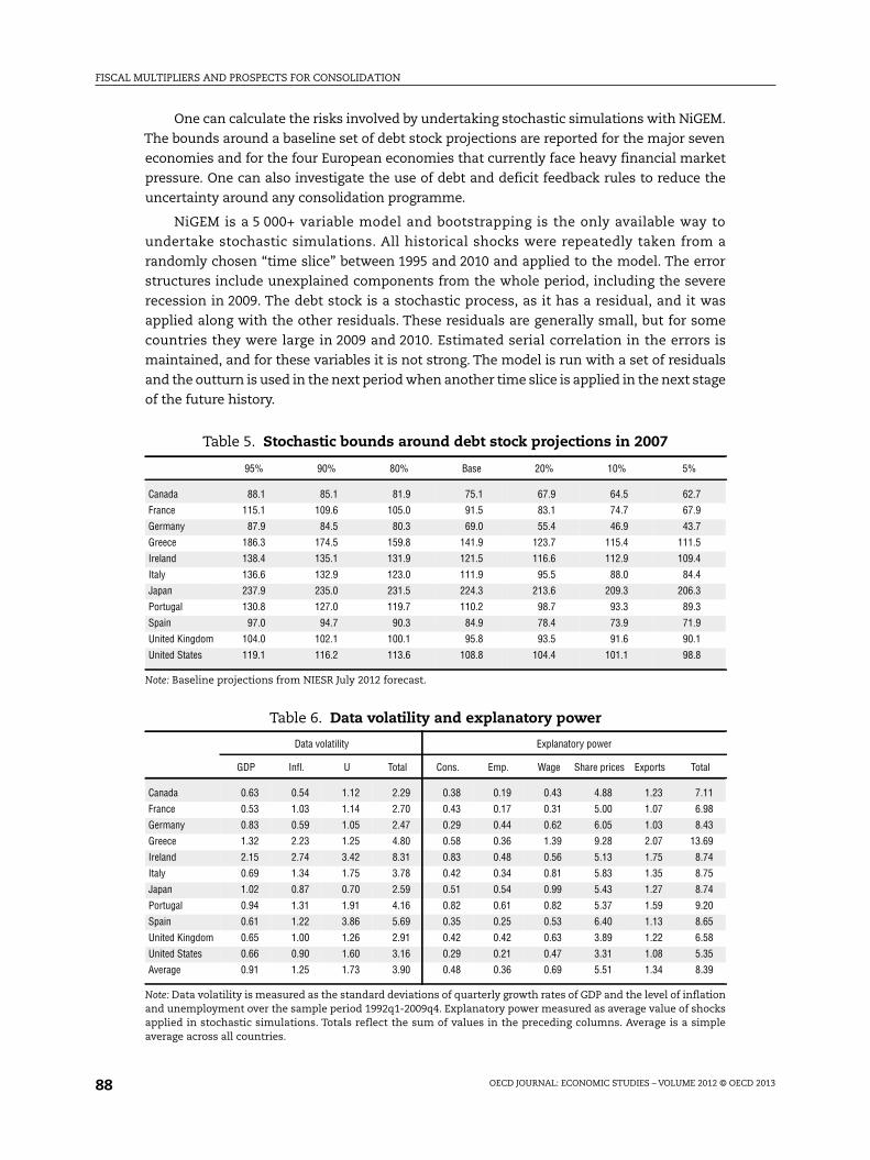
Table 5. Stochastic bounds around debt stock projections in 2007

95% 90% 80% Base 20% 10% 5%

Canada 88.1 85.1 81.9 75.1 67.9 64.5 62.7

France 115.1 109.6 105.0 91.5 83.1 74.7 67.9

Germany 87.9 84.5 80.3 69.0 55.4 46.9 43.7

Greece 186.3 174.5 159.8 141.9 123.7 115.4 111.5

Ireland 138.4 135.1 131.9 121.5 116.6 112.9 109.4

Italy 136.6 132.9 123.0 111.9 95.5 88.0 84.4

Japan 237.9 235.0 231.5 224.3 213.6 209.3 206.3

Portugal 130.8 127.0 119.7 110.2 98.7 93.3 89.3

Spain 97.0 94.7 90.3 84.9 78.4 73.9 71.9

United Kingdom 104.0 102.1 100.1 95.8 93.5 91.6 90.1

United States 119.1 116.2 113.6 108.8 104.4 101.1 98.8

Note: Baseline projections from NIESR July 2012 forecast.

Table 6. Data volatility and explanatory power

Data volatility Explanatory power

GDP Infl. U Total Cons. Emp. Wage Share prices Exports Total

Canada 0.63 0.54 1.12 2.29 0.38 0.19 0.43 4.88 1.23 7.11

France 0.53 1.03 1.14 2.70 0.43 0.17 0.31 5.00 1.07 6.98

Germany 0.83 0.59 1.05 2.47 0.29 0.44 0.62 6.05 1.03 8.43

Greece 1.32 2.23 1.25 4.80 0.58 0.36 1.39 9.28 2.07 13.69

Ireland 2.15 2.74 3.42 8.31 0.83 0.48 0.56 5.13 1.75 8.74

Italy 0.69 1.34 1.75 3.78 0.42 0.34 0.81 5.83 1.35 8.75

Japan 1.02 0.87 0.70 2.59 0.51 0.54 0.99 5.43 1.27 8.74

Portugal 0.94 1.31 1.91 4.16 0.82 0.61 0.82 5.37 1.59 9.20

Spain 0.61 1.22 3.86 5.69 0.35 0.25 0.53 6.40 1.13 8.65

United Kingdom 0.65 1.00 1.26 2.91 0.42 0.42 0.63 3.89 1.22 6.58

United States 0.66 0.90 1.60 3.16 0.29 0.21 0.47 3.31 1.08 5.35

Average 0.91 1.25 1.73 3.90 0.48 0.36 0.69 5.51 1.34 8.39

Note: Data volatility is measured as the standard deviations of quarterly growth rates of GDP and the level of inflationand unemployment over the sample period 1992q1-2009q4. Explanatory power measured as average value of shocksapplied in stochastic simulations. Totals reflect the sum of values in the preceding columns. Average is a simpleaverage across all countries.



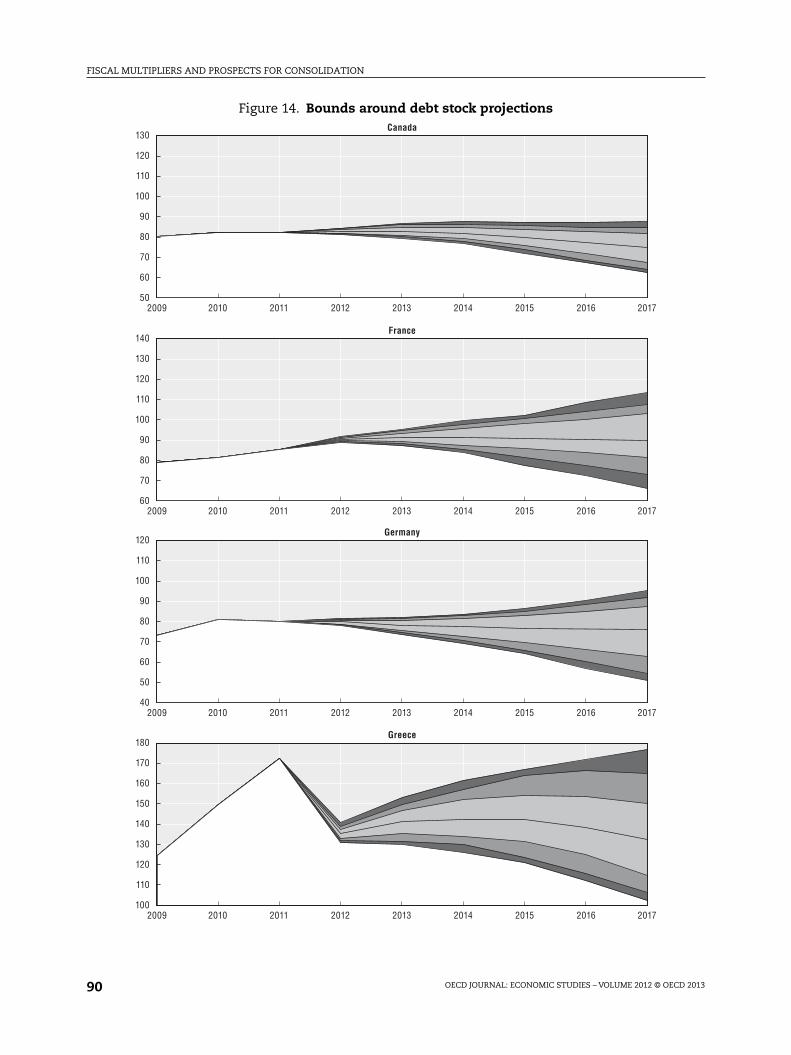
Stochastic simulation bounds were applied around the baselines from 2012q1

to 2028q1. For the first five years tax rates are fixed so that shock effects show up in the

deficit and not in the tax rate, and hence debt stocks can rise or fall without any reaction.

After 2016, tax rates respond to bring the debt stock back towards the target imposing a no-

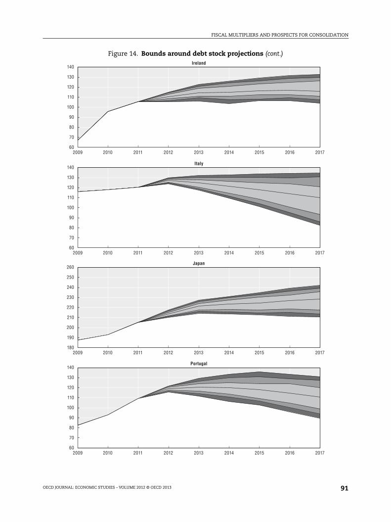
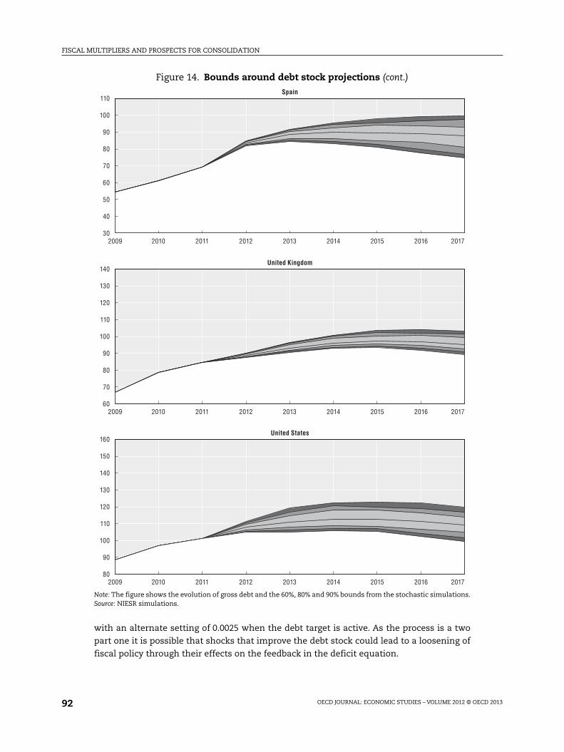
Ponzi game condition. Uncertainty bounds are plotted in Figure 14. Each figure gives the 80,

90 and 95% probability bounds around the debt stock projections. The baseline projections

are discussed in the July 2012 National Institute Economic Review.

Table 5 gives the values of the bounds for the debts stocks as a per cent of GDP for the

major seven economies and for Spain, Portugal, Ireland and Greece. In each case these are

the probability bounds for the debt stock if taxes do not increase in order to keep the stock

within bounds. The Greek debt stock could, on these projections lie somewhere

between 111 and 186% of GDP by 2017, whilst that in Japan (on a gross basis) could lie

somewhere between 206 and 238% of GDP. These bounds can be brought under control by

using feedback rules (see below).

As discussed above, the stochastic bounds around the central debt projections are a

combined reflections of three sources of uncertainty and volatility: the volatility inherent in

key historical data series themselves; the explanatory power of the equations; and the

persistence of shocks to the economy, for which Figure 9 above can act as a guide. In order to

distinguish between the uncertainty related to volatility in the data and uncertainty related

to the explanatory power of the model, Table 6 reports the standard deviations of three core

quarterly macro series (GDP growth, inflation and the unemployment rate) and the standard

deviation of the error (detrended and demeaned) on a set of key behavioural equations

underlying the model that reflect the shocks applied during the stochastic runs

(consumption, employment, wages, share prices and exports). The historical data for Greece,

Ireland and Spain are more volatile than for other countries, whereas it is relatively stable in

Canada, Germany and Japan. Even with volatile data, if the direction of volatility is

predictable, it may still be possible to build a model with a high degree of explanatory power.

The model with the lowest degree of explanatory power is Greece, where share price, exports

and wages are all relatively poorly explained by the NiGEM equation. The model with the

highest degree of explanatory power is the United States. These factors can help explain

some of the differences in the error bounds around the debt profiles illustrated in Figure 14.

5.1. Fiscal policy feedback rules

Fiscal policy feedback rules can either respond to the deviation of the deficit (gbr) from

its target (gbrt) or the deviation of the debt stock (gdr) from its target (gdrt), or both. The first

would be a proportional controller, the second an integral contoller and the third a

propotional and integral controller. The speed at which the debt stock returns to target

depends on the choice of the rule and its parameters, as does the uncertainty around the

target. The debt and deficit process is a two part one, with shocks occuring to deficits and to

debts separately, as not all shocks to the debt stock (bank failures, privatisations, licence

sales) affect the deficit. One can write the two equations as:

gbrt = a + (gbrt – 1 – gbrtt – 1) + (gdrt – gdrtt – 1) + t (2)

gdrt = gdrt – 1 – gbrt + t (3)

Feedbacks are included in the gbr equation (2), and either the deficit or debt targets or

both may be used. In NiGEM the instrument used is the direct tax rate, although it is also

possible to use other instruments. The default value for is set at 0.2 and that for is 0,



Figure 14. Bounds around debt stock projections

130

120

110

100

90

80

70

60

502009 2010 2011 2012 2013 2014 2015 2016 2017

140

130

120

110

100

90

80

70

602009 2010 2011 2012 2013 2014 2015 2016 2017

120

110

100

90

80

70

60

50

402009 2010 2011 2012 2013 2014 2015 2016 2017

180

170

160

150

140

130

120

110

1002009 2010 2011 2012 2013 2014 2015 2016 2017

Canada

France

Germany

Greece



Figure 14. Bounds around debt stock projections (cont.)

140

130

120

110

100

90

80

70

602009 2010 2011 2012 2013 2014 2015 2016 2017

140

130

120

110

100

90

80

70

602009 2010 2011 2012 2013 2014 2015 2016 2017

260

250

240

230

220

210

200

190

1802009 2010 2011 2012 2013 2014 2015 2016 2017

140

130

120

110

100

90

80

70

602009 2010 2011 2012 2013 2014 2015 2016 2017

Ireland

Italy

Japan

Portugal



with an alternate setting of 0.0025 when the debt target is active. As the process is a two

part one it is possible that shocks that improve the debt stock could lead to a loosening of

fiscal policy through their effects on the feedback in the deficit equation.

Figure 14. Bounds around debt stock projections (cont.)

Note: The figure shows the evolution of gross debt and the 60%, 80% and 90% bounds from the stochastic simulations.Source: NIESR simulations.

110

100

90

80

70

60

50

40

302009 2010 2011 2012 2013 2014 2015 2016 2017

140

130

120

110

100

90

80

70

602009 2010 2011 2012 2013 2014 2015 2016 2017

160

150

140

130

120

110

100

90

802009 2010 2011 2012 2013 2014 2015 2016 2017

Spain

United Kingdom

United States



A spending based fiscal consolidation of 1% of GDP in all euro area countries was

simulated, and stochastic bounds around the outcome calibrated under the assumption that

for the first five years taxes do not rise to pull the deficit back to target. These are the no

solvency rule bounds around this initial consolidation scenario, and one can compare the

bounds with those from a set of rules.

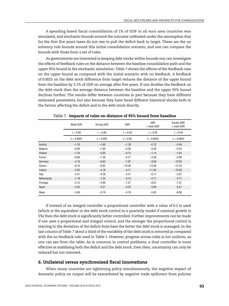
As governments are interested in keeping debt stocks within bounds one can investigate

the effects of feedback rules on the distance between the baseline consolidation path and the

upper 95% bound in the stochastic simulation. Table 7 shows the effects of the feedback case

on the upper bound as compared with the initial scenario with no feedback. A feedback

of 0.0025 on the debt stock difference from target reduces the distance of the upper bound

from the baseline by 3.1% of GDP on average after five years. If one doubles the feedback on

the debt stock then the average distance between the baseline and the upper 95% bound

declines further. The results differ between countries in part because they have different

estimated parameters, but also because they have faced different historical shocks both to

the factors affecting the deficit and to the debt stock directly.

If instead of an integral controller a proportional controller with a value of 0.2 is used

(which is the equivalent to the debt stock control in a quarterly model if nominal growth is

5%) then the debt stock is significantly better controlled. Further improvements can be made

if one uses a proportional and integral control, and the stronger the proportional control is

reacting to the deviation of the deficit from base the better the debt stock is managed. In the

last column of Table 7 about a third of the variablity of the debt stock is removed as compared

with the no feedback rule used in Table 5. However, progress across rules is not uniform, as

one can see from the table. As is common in control problems, a dual controller is more

effective at stabilising both the deficit and the debt stock. Even then, uncertainty can only be

reduced but not removed.

6. Unilateral versus synchronised fiscal innovationsWhen many countries are tightening policy simultaneously, the negative impact of

domestic policy on output will be exacerbated by negative trade spillovers from policies

Table 7. Impacts of rules on distance of 95% bound from baseline

Weak GDR Strong GDR GBRGBR

+ weak GDRDouble GBR+ weak GDR

= 0.00 = 0.00 = 0.20 = 0.20 = 0.40

= 0.0025 = 0.005 = 0.00 = 0.0025 = 0.0025

Austria –1.33 –1.60 –1.29 –2.12 –2.48

Belgium –0.83 –1.69 –3.05 –3.35 –3.54

Finland –1.44 –2.65 –0.75 –1.14 –1.64

France –0.66 –1.30 –4.27 –3.05 –3.56

Germany –4.19 –6.63 –7.87 –8.56 –10.50

Greece –6.16 –8.92 –10.26 –13.26 –12.35

Ireland –5.95 –4.78 –4.71 –11.05 –10.59

Italy –4.37 –4.29 –4.41 –6.17 –3.67

Netherlands –1.18 –1.34 –4.15 –2.71 –4.77

Portugal –4.15 –4.89 –7.57 –6.67 –7.37

Spain –3.42 –3.57 –4.25 –3.83 –5.57

Mean –3.06 –3.79 –4.78 –5.63 –6.00



abroad. This is partially offset, especially in the smaller economies in the euro area, by the

bigger impact of the joint action on ECB interest rate setting and more significant depreciation

of the exchange rate. In order to assess the impact of synchronised policy innovations, we re-

run the permanent spending shocks, which are reported in Table 4 above on a unilateral

basis, applying a 1% of GDP spending-based consolidation in all 18 countries simultaneously.

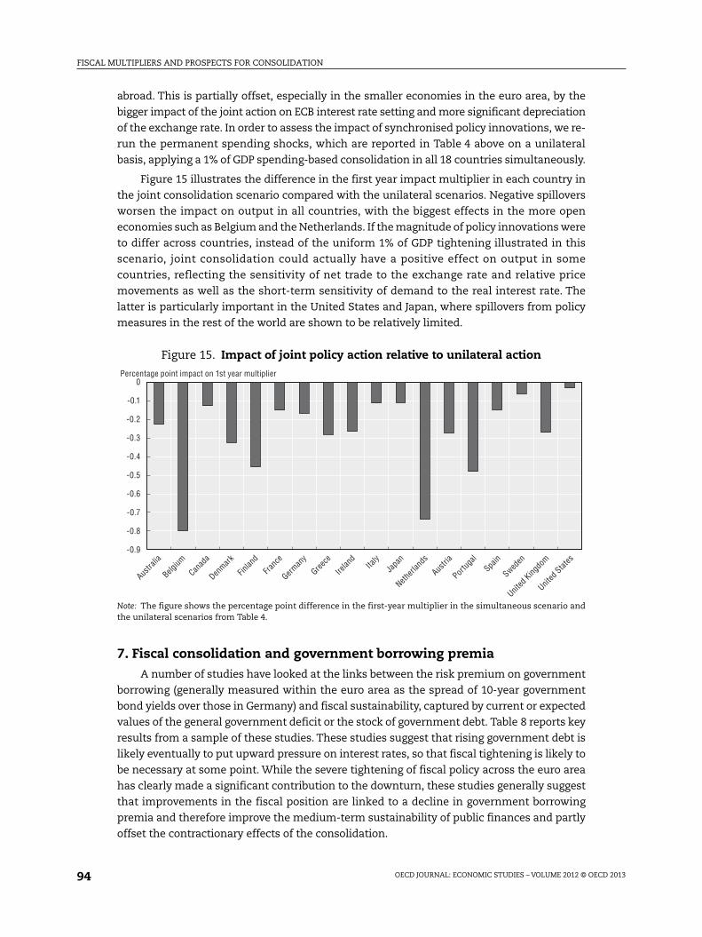
Figure 15 illustrates the difference in the first year impact multiplier in each country in

the joint consolidation scenario compared with the unilateral scenarios. Negative spillovers

worsen the impact on output in all countries, with the biggest effects in the more open

economies such as Belgium and the Netherlands. If the magnitude of policy innovations were

to differ across countries, instead of the uniform 1% of GDP tightening illustrated in this

scenario, joint consolidation could actually have a positive effect on output in some

countries, reflecting the sensitivity of net trade to the exchange rate and relative price

movements as well as the short-term sensitivity of demand to the real interest rate. The

latter is particularly important in the United States and Japan, where spillovers from policy

measures in the rest of the world are shown to be relatively limited.

7. Fiscal consolidation and government borrowing premiaA number of studies have looked at the links between the risk premium on government

borrowing (generally measured within the euro area as the spread of 10-year government

bond yields over those in Germany) and fiscal sustainability, captured by current or expected

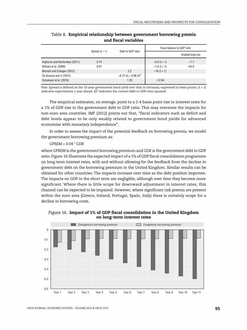
values of the general government deficit or the stock of government debt. Table 8 reports key

results from a sample of these studies. These studies suggest that rising government debt is

likely eventually to put upward pressure on interest rates, so that fiscal tightening is likely to

be necessary at some point. While the severe tightening of fiscal policy across the euro area

has clearly made a significant contribution to the downturn, these studies generally suggest

that improvements in the fiscal position are linked to a decline in government borrowing

premia and therefore improve the medium-term sustainability of public finances and partly

offset the contractionary effects of the consolidation.

Figure 15. Impact of joint policy action relative to unilateral action

Note: The figure shows the percentage point difference in the first-year multiplier in the simultaneous scenario andthe unilateral scenarios from Table 4.

0

-0.1

-0.2

-0.3

-0.4

-0.5

-0.6

-0.7

-0.8

-0.9

Austra

lia

Belg

ium

Can

ada

Den

mark

Finl

and

Fran

ce

Germ

any

Gree

ce

Irela

nd It

aly

Japa

n

Netherl

ands

Aus

tria

Por

tugal

Spa

in

Swed

en

Unit

ed King

dom

Unit

ed Stat

es

Percentage point impact on 1st year multiplier



The empirical estimates, on average, point to a 2-4 basis point rise in interest rates for

a 1% of GDP rise in the government debt to GDP ratio. This may overstate the impacts for

non-euro area countries. IMF (2012) points out that, “fiscal indicators such as deficit and

debt levels appear to be only weakly related to government bond yields for advanced

economies with monetary independence”.

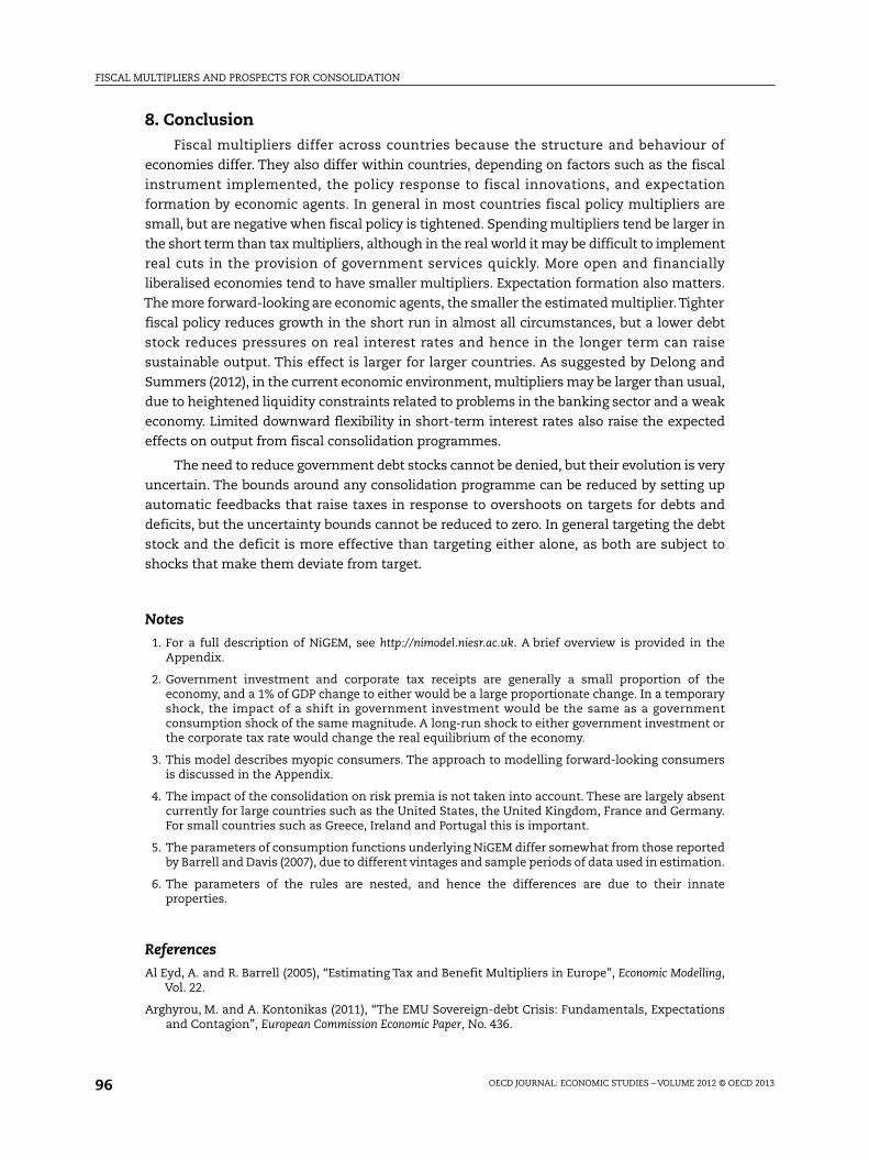
In order to assess the impact of the potential feedback on borrowing premia, we model

the government borrowing premium as:

GPREM = 0.04 * GDR

where GPREM is the government borrowing premium and GDR is the government debt to GDP

ratio. Figure 16 illustrates the expected impact of a 1% of GDP fiscal consolidation programme

on long-term interest rates, with and without allowing for the feedback from the decline in

government debt on the borrowing premium in the United Kingdom. Similar results can be

obtained for other countries. The impacts increase over time as the debt position improves.

The impacts on GDP in the short term are negligible, although over time they become more

significant. Where there is little scope for downward adjustment in interest rates, this

channel can be expected to be impaired. However, where significant risk premia are present

within the euro area (Greece, Ireland, Portugal, Spain, Italy) there is certainly scope for a

decline in borrowing costs.

Table 8. Empirical relationship between government borrowing premiaand fiscal variables

Spread (t – 1) Debt to GDP ratioFiscal balance to GDP ratio

Implied long-run

Arghyrou and Kontonikas (2011) 0.74 –2.0 (t + 1) –7.7

Attinasi et al. (2009) 0.97 –1.6 (t + 1) –54.9

Bernoth and Erdogan (2012) 2.2 –16 (t + 1)

De Grauwe and Ji (2012) –6.12 (t) + 0.08 (t)2

Schuknect et al. (2010) 1.25 –12.64

Note: Spread is defined as the 10-year government bond yield over that in Germany, expressed in basis points. (t + 1)indicates expectations 1 year ahead. (t)2 indicates the current debt to GDP ratio squared.

Figure 16. Impact of 1% of GDP fiscal consolidation in the United Kingdomon long-term interest rates

0

-0.1

-0.2

-0.3

-0.4

-0.5

-0.6

Endogenous borrowing premium Exogenous borrowing premium

Year 1 Year 2 Year 3 Year 4 Year 5 Year 6 Year 7 Year 8 Year 9 Year 10 Year 11



8. ConclusionFiscal multipliers differ across countries because the structure and behaviour of

economies differ. They also differ within countries, depending on factors such as the fiscal

instrument implemented, the policy response to fiscal innovations, and expectation

formation by economic agents. In general in most countries fiscal policy multipliers are

small, but are negative when fiscal policy is tightened. Spending multipliers tend be larger in

the short term than tax multipliers, although in the real world it may be difficult to implement

real cuts in the provision of government services quickly. More open and financially

liberalised economies tend to have smaller multipliers. Expectation formation also matters.

The more forward-looking are economic agents, the smaller the estimated multiplier.Tighter

fiscal policy reduces growth in the short run in almost all circumstances, but a lower debt

stock reduces pressures on real interest rates and hence in the longer term can raise

sustainable output. This effect is larger for larger countries. As suggested by Delong and

Summers (2012), in the current economic environment, multipliers may be larger than usual,

due to heightened liquidity constraints related to problems in the banking sector and a weak

economy. Limited downward flexibility in short-term interest rates also raise the expected

effects on output from fiscal consolidation programmes.

The need to reduce government debt stocks cannot be denied, but their evolution is very

uncertain. The bounds around any consolidation programme can be reduced by setting up

automatic feedbacks that raise taxes in response to overshoots on targets for debts and

deficits, but the uncertainty bounds cannot be reduced to zero. In general targeting the debt

stock and the deficit is more effective than targeting either alone, as both are subject to

shocks that make them deviate from target.

Notes

1. For a full description of NiGEM, see http://nimodel.niesr.ac.uk. A brief overview is provided in theAppendix.

2. Government investment and corporate tax receipts are generally a small proportion of theeconomy, and a 1% of GDP change to either would be a large proportionate change. In a temporaryshock, the impact of a shift in government investment would be the same as a governmentconsumption shock of the same magnitude. A long-run shock to either government investment orthe corporate tax rate would change the real equilibrium of the economy.

3. This model describes myopic consumers. The approach to modelling forward-looking consumersis discussed in the Appendix.

4. The impact of the consolidation on risk premia is not taken into account. These are largely absentcurrently for large countries such as the United States, the United Kingdom, France and Germany.For small countries such as Greece, Ireland and Portugal this is important.

5. The parameters of consumption functions underlying NiGEM differ somewhat from those reportedby Barrell and Davis (2007), due to different vintages and sample periods of data used in estimation.

6. The parameters of the rules are nested, and hence the differences are due to their innateproperties.

References

Al Eyd, A. and R. Barrell (2005), “Estimating Tax and Benefit Multipliers in Europe”, Economic Modelling,Vol. 22.

Arghyrou, M. and A. Kontonikas (2011), “The EMU Sovereign-debt Crisis: Fundamentals, Expectationsand Contagion”, European Commission Economic Paper, No. 436.



Attinasi, M.G., C. Checherita and C. Nickel (2009), “What Explains the Surge in Euro Area SovereignSpreads during the Financial Crisis of 2007-09?”, European Central Bank Working Paper, No. 1131.

Auerbach, A.J. and Y. Gorodnichenko (2012), “Fiscal Multipliers in Recession and Expansion”, AmericanEconomic Journal: Economic Policy, 4(2), pp. 1-27.

Barrell, R, D. Holland and A.I. Hurst (2007), “Correcting US Imbalances”, NIESR Discussion Paper, No. 290.

Barrell, R. (2001), “Fiscal Policy in the Longer Term”, National Institute Economic Review, No. 217, pp. F4-F10.

Barrell, R. and E.P. Davis (2007), “Financial Liberalisation, Consumption and Wealth Effects in SevenOECD Countries”, Scottish Journal of Political Economy, Vol. 54, No. 2.

Barrell, R. and K. Dury (2003), “Asymmetric Labour Markets in a Converging Europe: Do DifferencesMatter?”, National Institute Economic Review, No. 183.

Barrell, R., A.I. Hurst and J. Mitchell (2007), “Uncertainty Bounds for Cyclically-Adjusted BudgetBalances”, in M. Larch and L.N. Martins (eds.), Fiscal Indicators, European Commission, Brussels.

Barrell, R., S.G. Hall and A.I. Hurst (2006), “Evaluating Policy Feedback Rules Using the Joint DensityFunction of a Stochastic Model”, Economics Letters, Vol. 93, No. 1.

Barrell, R., T. Fic and I. Liadze (2009), “Fiscal Policy Effectiveness in the Banking Crisis”, National InstituteEconomic Review, No. 207.

Bernoth, K. and B. Erdogan (2012), “Sovereign Bond Yield Spreads: A Time-Varying CoefficientApproach”, Journal of International Money and Finance, 31, pp. 639-56.

Corsetti, G., K. Kuester, A. Meier and G. Meuller (2012), “Sovereign Risk, Fiscal Policy andMacroeconomic Stability”, IMF Working Paper, 12/33.

De Grauwe, P. and Y. Ji (2012), “Mispricing of Sovereign Risk and Multiple Equilibria in the Eurozone”,CEPS Working Document, No. 361.

DeLong, J.B. and L.H. Summers (2012), “Fiscal Policy in a Depressed Economy”, Brookings Papers onEconomic Activity.

Harrison, R. et al. (2005), The Bank of England Quarterly Model, Bank of England, London.

IMF (2012), United Kingdom 2012 Article IV Consultation, Country Report, No. 12/190.

Schuknecht, L., J. von Hagen and G. Wolswijk (2010), “Government Bond Risk Premiums in the EURevisited. The Impact of the Financial Crisis”, European Central Bank Working Paper, No. 1152.



APPENDIX

The NiGEM model

The National Institute’s global econometric model (NiGEM) can be used in a number of

ways, from a backward-looking structural model to a version that has similar long-run

properties as the dynamic stochastic general equilibrium models used by institutions such

as the Bank of England.1 Although the model is estimated it has a strong role for expectations,

and it is also flexible, as it can be run under different models of expectations formation,

depending upon the thought experiment being undertaken. Financial markets normally

follow arbitrage conditions and they are forward looking. The exchange rate, the long-term

interest rate and the equity price will all jump in response to news about future events. Fiscal

policy making involves gradually adjusting direct taxes to maintain the deficit on target, but

it is assumed that taxes have no direct effect on labour supply decisions. Monetary policy

making involves targeting inflation with an integral control from the price level, as discussed

in Barrell, Hall and Hurst (2006) and inflation settles at its target in all simulations. Some of

the key features of the model that determine the outturns of the simulation studies are

detailed further below.

Production and investmentGDP (Y) is determined in the long run by supply factors, and the economy is open and

has perfect capital mobility. The production function has a constant elasticity of substitution

between factor inputs, where output depends on capital (K) and on labour services (L), which

is a combination of the number of persons in work and the average hours of those persons.

Technical progress (tech) is assumed to be labour augmenting and independent of the policy

innovations considered here. Fiscal tightening measures have a negative impact on GDP in

the short run, but unless they permanently shift the desired level of capital, labour supply or

technical progress, these effects dissipate over time and will not affect the level of output

over the longer term.

(1)

Equation (1) constitutes the theoretical background for the specifications of the factor

demand equations. Demand for capital is determined by profit maximisation of firms,

implying that the long-run capital output ratio depends on the real user cost of capital. In

general, forward-looking behaviour in production is assumed, and so investment depends on

expected trend output four years ahead and the forward-looking user cost of capital.

However, the capital stock does not adjust instantly, as there are costs involved in doing so

that are represented by estimated speeds of adjustment.The user cost of capital is influenced

by corporate taxes, depreciation and risk premia and is a weighted average of the cost of

� �� /1)))(1()(( � techLLeKY



equity finance and the margin adjusted long real rate. Fiscal innovations through the

corporate tax rate or through government investment can permanently shift the level of the

capital stock, and through this shift the long-run level of potential output.

Labour market and wage settingDemand for labour is also determined by profit maximisation of firms, implying that the

long-run labour-output ratio depends on real wage costs and technical progress. Labour

supply is modelled as essentially exogenous, determined by demographics and an

exogenous rate of participation.

The equilibrium level of unemployment is the outcome of a bargaining process in the

labour market, as discussed in Barrell and Dury (2003). NiGEM assumes that employers have

a right to manage, and hence the bargain in the labour market is over the real wage. Real

wages, therefore, depend on the level of trend labour productivity as well as the rate of

unemployment. The dynamics of the labour market depend on the estimated speed of

adjustments in the wage and labour demand equations, and the extent to which short-term

wage dynamics depend on (rational) expectations of future inflation and on current or past

inflation. The degree of price inertia/real wage flexibility in the economy is an important

factor underlying the different dynamic profiles observed in response to a fiscal innovation.

Consumer behaviourAs Barrell and Davis (2007) show, both the level of total asset based wealth [ln(TAW) or

ln(NW + HW)] and changes in financial [(dln(NW)] and especially housing wealth [dln(HW)]

will affect consumption (C).2 Their estimates suggest that the impact of changes in housing

wealth have five times the impact of changes in financial wealth in the short run, although

long-run effects are the same. Barrell and Davis (2007) also show that adjustment to the long-

run equilibrium shows some inertia as well.3 Al Eyd and Barrell (2005) discuss borrowing

constraints, and investigate the role of changes in the number of borrowing constrained

households. It is common to associate the severity of borrowing constraints with the

coefficient on changes in current real incomes [dln(RPDI)] in the equilibrium correction

equation for consumption (parameter b1). These coefficients are important in evaluating

impact multipliers. They may also be time-varying and dependent on the state of the

economy, as the number of liquidity constrained consumers will rise during an economic

downturn.This may be a key channel through which fiscal multipliers become dependent on

the state of the economy, as suggested by e.g. Delong and Summers (2012). One can write the

equation for dln(C) as:

(2)

where the long-run relationship between ln(C) and ln(RPDI) and ln(TAW) determine the

equilibrium savings rate, and this relationship forms the long-run attractor in an equilibrium

correction relationship.The logarithmic approximation is explained in Barrell and Davis (2007).

Operating in forward-looking consumption mode, consumers react to the present

discounted value of their expected future income streams, which is approximated by total

wealth (TW), although borrowing constraints may limit their consumption to their personal

disposable income in the short run. Total human wealth is defined as:

TWt = Yt – Tt + TWt + 1 / [(1 + rrt)(1 + myt)] (3)

� � � � � � � � � �� ttt

tttt

HWdbNWdbRPDIdbRPDIbTAWbaCCd

lnlnlnln1lnlnln

321

10101

� �



Y is real income, T are real taxes, and the subscript t + 1 indicates an expected variable which

is discounted by the real interest rate rrt and by the myopia premium of consumers, myt. The

equation represents an infinite forward recursion, and permanent income is the sustainable

flow from this stock. Fiscal multipliers are sensitive to the expectations formation of

households. Fully forward-looking consumers anticipate that current consolidation

measures may entail lower tax rates in the medium to longer term, offsetting some of the

negative impact on consumption in the short term, as households aim to smooth their

consumption path. Multipliers are higher with myopic consumers.

Government sectorIn order to evaluate multipliers a reasonably disaggregated description of both spending

and tax receipts is needed. Corporate (CTAX) and personal (TAX) direct taxes and indirect

taxes (MTAX) on spending are modelled, along with government spending on investment (GI)

and on current consumption (GC), and transfers (TRAN) and government interest payments

(GIP) are separately identified. Each source of taxes has an equation applying a tax rate to a

tax base (profits, personal incomes or consumption). As a default, government spending on

investment and consumption are rising in line with trend output in the long run, with

delayed adjustment to changes in the trend. They are re-valued in line with the consumers’

expenditure deflator (CED). Government interest payments are driven by a perpetual

inventory of accumulated debts. Transfers to individuals are composed of three elements,

with those for the inactive of working age and the retired depending upon observed

replacement rates. Spending less receipts gives the budget deficit (BUD), which adds to the

debt stock.

BUD = CED*(GC + GI) + TRAN + GIP – TAX – CTAX – MTAX (4)

It has to be considered how the government deficit (BUD) is financed. Either money (M)

or bond financing (DEBT) are allowed:

BUD = d(M) + d(DEBT) (5)

and rearranging gives:

DEBT = DEBTt – 1 + BUD – d(M) (6)

In all policy analyses a tax rule is used to ensure that governments remain solvent in the long

run. The default rule is applied to the personal direct tax rate, which is adjusted

endogenously to bring the government deficit into line with a specified target. This ensures

that the deficit and debt stock return to sustainable levels after a shock. A debt stock target

can also be implemented and this is discussed below. The income tax rate (TAXR) equation is

of the form:

TAXR = f(target debt or deficit ratio – actual debt or deficit ratio) (7)

If the government budget deficit is above the target (e.g. 3% of GDP and the target is 1%), then

the income tax rate is increased.

Monetary policyA tighter fiscal policy will allow short-term interest rates to be lower now and in the future

if there is no change to the monetary policy target, and hence long-term interest rates will be

lower now. Barrell (2001) reviews evidence on expansionary fiscal contractions, and concludes

they are exceptionally rare. Interest rates are set by the monetary authority in relation to a

targeting regime, where policy interest rates are set in relation to a rule that is normally forward



looking. Fiscal multipliers depend on the assumed targeting regime, and the extent to which

fiscal innovations are accommodated by monetary policy in the short term.We distinguish two

types of rules, those that target only inflation and those that target the price level or a nominal

variable such as GDP or the money stock. During the “Great Moderation” era, central bankers

and many economists became convinced that they had changed the world they lived in by

adopting simple feedback rules for monetary policy in combination with rules for fiscal policy

that kept debt in bounds. The simple feedback rule was based on the Taylor Rule (TR) that

suggests that when inflation increases, the central bank should increase the interest rate more

than in proportion to the rise in inflation, and hence the real interest rate would rise and help

choke off demand. In a forward-looking world it is possible to improve on this principal. If

agents see the central bank as fully credible, then the announcement of a price level target

(PLT), rather than just an inflation target, will stabilise fluctuations in output and in inflation.

A price level targeting central bank will loosen policy more rapidly as it has to get the price level

back to target. The converse will be true in a boom. These two feedback rules are shown in

equation (8) below, with int being the intervention rate, ssr being the steady state (endogenous)

real interest rate, og being the output gap, inf and inft being the inflation rate and the target, and

P and PT being the price level and the price level target.

intt = a0 + a1ssrt + a2ogt + a3(inft + 1 – inft) + a4(Pt – PTt) (8)

In a Taylor Rule, a0 is zero, a1 is 1.0, a2 is 0.5, a3 is 1.5 and a4 is zero, whilst in a PLT regime

a1 is zero, a2 is also zero, and a3 is set to 0.7 and a4 to 0.4. The PLT rule has the advantage of

working only on observables.The same is true of a two pillar strategy as embraced by the ECB.

The bank responds to deviations of inflation from target and also deviations of a nominal

aggregate (NOM) – the money stock for instance – as described in the equation:

intt = b0 + b1(inft + 1 – inft) + b2(NOMt – NOMTt) (9)

Forward looking financial marketsA deflationary shock such as a fiscal tightening will have a weaker interest rate response

under a Taylor Rule than under price level targeting, and both may be weaker than a two

pillar rule. If actors know the rule is in place then they will form expectations of the future

path of short rates, and this will cause the current long rate to change, along with the

exchange rate and the equity price. If fiscal policy is expected to be tightened in the future

then long rates will fall now, increasing the offset, and perhaps even inducing a short-term

expansion of output. Forward-looking long rates (LR) should be related to expected future

short-term rates:

(10)

Forward-looking equity prices (EQP) are related to future profits (PR) in a forward recursion

where eprem is the equity premium:

(11)

The exchange rate depends on the expected future path of interest rates and the

exchange rate risk premia, solving an uncovered interest parity condition, so that the

expected change in the exchange rate is given by the difference in the interest earned on

assets held in local and foreign currencies:

(12)

� � � �� Tj

Tjtt intLR 1

/111

� �� tt

ttt epremint

EQPPREQP

�

111

� �tt

ttt rpee ��

�

��

�

� 1int1int1 *

1



where et is the bilateral exchange rate at time t (defined as domestic currency per unit of

foreign currency), intt is the short-term nominal interest rate at home set in line with a policy

rule, intt* is the interest rate abroad and rpt is the exchange rate risk premium.

Notes

1. The Bank of England Quarterly model is discussed in Harrison et al. (2005). NiGEM is discussed in Barrell,Holland and Hurst (2007), Barrell, Hurst and Mitchell (2007) and in other papers at www.niesr.ac.uk.NiGEM does not impose maximising equilibrium conditions in the same way as Dynamic StochasticGeneral Equilibrium models, but has the same steady-state equilibrium properties.

2. Throughout d is the change operator and ln is the natural logarithm.

3. While the approach underlying NiGEM consumption equations is the same used in Barrell andDavis (2007), the estimated parameters differ, due to different vintages and sample periods of dataused in estimation.

Documents

prospects for consolidation Fiscal multipliers and - OECD. · PDF fileprospects for consolidation Ray Barrell, Dawn Holland, Ian Hurst Please cite this article as: Barrell ... differ