Embed Size (px)
Citation preview

NORTH SEA STUDY OCCASIONAL PAPER
No. 134
Prospective Returns to Exploration
in the UKCS
with Cost Reductions and Tax Incentives
Professor Alexander G. Kemp
and
Linda Stephen
December, 2015
Aberdeen Centre for Research in Energy Economics and
Finance (ACREEF) © A.G. Kemp and L. Stephen

ii
ISSN 0143-022X
NORTH SEA ECONOMICS
Research in North Sea Economics has been conducted in the Economics Department
since 1973. The present and likely future effects of oil and gas developments on the
Scottish economy formed the subject of a long term study undertaken for the Scottish
Office. The final report of this study, The Economic Impact of North Sea Oil on
Scotland, was published by HMSO in 1978. In more recent years further work has
been done on the impact of oil on local economies and on the barriers to entry and
characteristics of the supply companies in the offshore oil industry.
The second and longer lasting theme of research has been an analysis of licensing and
fiscal regimes applied to petroleum exploitation. Work in this field was initially
financed by a major firm of accountants, by British Petroleum, and subsequently by
the Shell Grants Committee. Much of this work has involved analysis of fiscal
systems in other oil producing countries including Australia, Canada, the United
States, Indonesia, Egypt, Nigeria and Malaysia. Because of the continuing interest in
the UK fiscal system many papers have been produced on the effects of this regime.
From 1985 to 1987 the Economic and Social Science Research Council financed
research on the relationship between oil companies and Governments in the UK,
Norway, Denmark and The Netherlands. A main part of this work involved the
construction of Monte Carlo simulation models which have been employed to
measure the extents to which fiscal systems share in exploration and development
risks.
Over the last few years the research has examined the many evolving economic issues
generally relating to petroleum investment and related fiscal and regulatory matters.
Subjects researched include the economics of incremental investments in mature oil
fields, economic aspects of the CRINE initiative, economics of gas developments and
contracts in the new market situation, economic and tax aspects of tariffing,
economics of infrastructure cost sharing, the effects of comparative petroleum fiscal
systems on incentives to develop fields and undertake new exploration, the oil price
responsiveness of the UK petroleum tax system, and the economics of
decommissioning, mothballing and re-use of facilities. This work has been financed
by a group of oil companies and Scottish Enterprise, Energy. The work on CO2
Capture, EOR and storage was financed by a grant from the Natural Environmental
Research Council (NERC) in the period 2005 – 2008.
For 2015 the programme examines the following subjects:
i. Investment Uplift for SC
ii. Cluster Allowance for SC
iii. PRT Rage Changes
iv. SC Rate Changes
v. Exploration Incentives
vi. Taxation of Infrastructure
iii
vii. Price, Cost and Tax Sensitivity of Activity in the UKCS
viii. EOR (including CO2 EOR)
ix. Economics of Marginal and Sub-Marginal Fields and New Technologies
x. Discount Rates and Appropriate Investment Uplift in Project Investment
Decision Making
xi. Economic Aspects of Decommissioning
The authors are solely responsible for the work undertaken and views expressed. The
sponsors are not committed to any of the opinions emanating from the studies.
Papers are available from:
The Secretary (NSO Papers)
University of Aberdeen Business School
Edward Wright Building
Dunbar Street
Aberdeen A24 3QY
Tel No: (01224) 273427
Fax No: (01224) 272181
Email: [email protected]
Recent papers published are:
OP 98 Prospects for Activity Levels in the UKCS to 2030: the 2005
Perspective
By A G Kemp and Linda Stephen (May 2005), pp. 52
£20.00
OP 99 A Longitudinal Study of Fallow Dynamics in the UKCS
By A G Kemp and Sola Kasim, (September 2005), pp. 42
£20.00
OP 100 Options for Exploiting Gas from West of Scotland
By A G Kemp and Linda Stephen, (December 2005), pp. 70
£20.00
OP 101 Prospects for Activity Levels in the UKCS to 2035 after the
2006 Budget
By A G Kemp and Linda Stephen, (April 2006) pp. 61
£30.00
OP 102 Developing a Supply Curve for CO2 Capture, Sequestration and
EOR in the UKCS: an Optimised Least-Cost Analytical
Framework
By A G Kemp and Sola Kasim, (May 2006) pp. 39
£20.00
OP 103 Financial Liability for Decommissioning in the UKCS: the
Comparative Effects of LOCs, Surety Bonds and Trust Funds
By A G Kemp and Linda Stephen, (October 2006) pp. 150
£25.00
OP 104 Prospects for UK Oil and Gas Import Dependence
By A G Kemp and Linda Stephen, (November 2006) pp. 38
£25.00

iv
OP 105 Long-term Option Contracts for CO2 Emissions
By A G Kemp and J Swierzbinski, (April 2007) pp. 24
£25.00
OP 106 The Prospects for Activity in the UKCS to 2035: the 2007
Perspective
By A G Kemp and Linda Stephen (July 2007) pp.56
£25.00
OP 107 A Least-cost Optimisation Model for CO2 capture
By A G Kemp and Sola Kasim (August 2007) pp.65
£25.00
OP 108 The Long Term Structure of the Taxation System for the UK
Continental Shelf
By A G Kemp and Linda Stephen (October 2007) pp.116
£25.00
OP 109 The Prospects for Activity in the UKCS to 2035: the 2008
Perspective
By A G Kemp and Linda Stephen (October 2008) pp.67
£25.00
OP 110 The Economics of PRT Redetermination for Incremental
Projects in the UKCS
By A G Kemp and Linda Stephen (November 2008) pp. 56
£25.00
OP 111 Incentivising Investment in the UKCS: a Response to
Supporting Investment: a Consultation on the North Sea Fiscal
Regime
By A G Kemp and Linda Stephen (February 2009) pp.93
£25.00
OP 112 A Futuristic Least-cost Optimisation Model of CO2
Transportation and Storage in the UK/ UK Continental Shelf
By A G Kemp and Sola Kasim (March 2009) pp.53
£25.00
OP 113 The Budget 2009 Tax Proposals and Activity in the UK
Continental Shelf (UKCS)
By A G Kemp and Linda Stephen (June 2009) pp. 48
£25.00
OP 114 The Prospects for Activity in the UK Continental Shelf to 2040:
the 2009 Perspective
By A G Kemp and Linda Stephen (October 2009) pp. 48
£25.00
OP 115 The Effects of the European Emissions Trading Scheme (EU
ETS) on Activity in the UK Continental Shelf (UKCS) and CO2
Leakage
By A G Kemp and Linda Stephen (April 2010) pp. 117
£25.00
OP 116 Economic Principles and Determination of Infrastructure Third
Party Tariffs in the UK Continental Shelf (UKCS)
By A G Kemp and Euan Phimister (July 2010) pp. 26
OP 117 Taxation and Total Government Take from the UK Continental
Shelf (UKCS) Following Phase 3 of the European Emissions

v
Trading Scheme (EU ETS)
By A G Kemp and Linda Stephen (August 2010) pp. 168
OP 118 An Optimised Illustrative Investment Model of the Economics
of Integrated Returns from CCS Deployment in the UK/UKCS
BY A G Kemp and Sola Kasim (December 2010) pp. 67
OP 119 The Long Term Prospects for Activity in the UK Continental
Shelf
BY A G Kemp and Linda Stephen (December 2010) pp. 48
OP 120 The Effects of Budget 2011 on Activity in the UK Continental
Shelf
BY A G Kemp and Linda Stephen (April 2011) pp. 50
OP 121 The Short and Long Term Prospects for Activity in the UK
Continental Shelf: the 2011 Perspective
BY A G Kemp and Linda Stephen (August 2011) pp. 61
OP 122 Prospective Decommissioning Activity and Infrastructure
Availability in the UKCS
BY A G Kemp and Linda Stephen (October 2011) pp. 80
OP 123 The Economics of CO2-EOR Cluster Developments in the UK
Central North Sea/ Outer Moray Firth
BY A G Kemp and Sola Kasim (January 2012) pp. 64
OP 124 A Comparative Study of Tax Reliefs for New Developments in
the UK Continental Shelf after Budget 2012
BY A G Kemp and Linda Stephen (July 2012) pp.108
OP 125 Prospects for Activity in the UK Continental Shelf after Recent
Tax Changes: the 2012 Perspective
BY A G Kemp and Linda Stephen (October 2012) pp.82
OP 126 An Optimised Investment Model of the Economics of Integrated
Returns from CCS Deployment in the UK/UKCS
BY A G Kemp and Sola Kasim (May 2013) pp.33
OP 127 The Full Cycle Returns to Exploration in the UK Continental
Shelf
BY A G Kemp and Linda Stephen (July 2013) pp.86
OP 128 Petroleum Taxation for the Maturing UK Continental Shelf
(UKCS)
BY A G Kemp, Linda Stephen and Sola Kasim (October 2014)
pp.94
OP 129 The Economics of Enhanced Oil Recovery (EOR) in the UKCS
and the Tax Review

vi
BY A G Kemp and Linda Stephen (November 2014) pp.47
OP 130 Price Sensitivity, Capital Rationing and Future Activity in the
UK Continental Shelf after the Wood Review
BY A G Kemp and Linda Stephen (November 2014) pp.41
OP 131 Tax Incentives for CO2-EOR in the UK Continental Shelf
BY A G Kemp and Sola Kasim (December 2014) pp. 49
OP
132
The Investment Allowance in the Wider Context of the UK
Continental Shelf in 2015: A Response to the Treasury
Consultation
BY A G Kemp and Linda Stephen (February 2015) pp. 27
OP 133 The Economics of Exploration in the UK Continental Shelf: the
2015 Perspective
BY A G Kemp and Linda Stephen (August 2015) pp. 71
OP 134 Prospective Returns to Exploration in the UKCS with Cost
Reductions and Tax Incentives
BY A G Kemp and Linda Stephen (December 2015) pp.81

vii
Prospective Returns to Exploration in the UKCS with Cost
Reductions and Tax Incentives
Professor Alexander G. Kemp and Linda Stephen
Contents Page
1. Introduction and Context………………………..……………1
2. Methodology and Assumptions………………………………….2
3. Results .…………………………………………………………7
A. Investment Allowance Eligible for All Exploration Costs
(a) Investor in Tax-Paying Position, Fast Cycle Time…………7
(b) Project Investor, Fast Cycle Time…………………………14
B. Tax Credit for Exploration
(a) Project Investor, Fast Cycle Time………………………....19
C. Investment Allowance Limited to Successful Exploration
(a) Investor in Tax-Paying Position, Fast Cycle Time………..24
(b) Project Investor, Fast Cycle Time…………………………28
D. Immediate Relief for Investment Allowance
(a) Investor in Tax-Paying Position, Fast Cycle Time………..33
E. Interest on Unutilised IA from Time of Eligibility for Activation
(a) Project Investor, Fast Cycle Time…………………………36
F. Investment Allowance Eligible for All Exploration Costs
(a) Investor in Tax-Paying Position, Slow Cycle Time……….40
(b) Project Investor, Slow Cycle Time………………………..47
G. Tax Credit for Exploration Costs
(a) Project Investor, Slow Cycle Time………………………..51
H. Investment Allowance Restricted to Successful Exploration
(a) Investor in Tax-Paying Position, Slow Cycle Time……….55
(b) Project Investor, Slow Cycle Time………………………..59
I. Immediate Relief for IA
(a) Investor in Tax-Paying Position, Slow Cycle Time……….63

viii
J. Interest on Unutilised IA from Time of Eligibility of Activation
(a) Project Investor, Slow Cycle Time…………….………….67
K. Comparison of Results………………………….…………….71
4. Summary and Conclusions……………………………………77

1
Prospective Returns to Exploration in the UKCS with
Cost Reductions and Tax Incentives
Professor Alexander G. Kemp
and
Linda Stephen
1. Introduction and Context
Exploration activity in the UK Continental Shelf (UKCS) has been falling
for some years, even when the oil price has been very high. This century
the average annual number of exploration wells drilled has been 25.8 with
the maximum being 44 in 2008 and the lowest 14 in both 2013 and 2014.
The figure for 2015 may will be lower. The average number of appraisal
wells drilled this century has been 36.5, with the highest being 77 in 2007
and only 18 in 2014. The figure for 2015 will be even lower. The low
figures for 2014 are arguably not primarily the consequence of the
collapse in the oil price in the later part of the year. Other factors
including the very high cost of drilling wells and relatively low views of
prospectivity are also likely to have influenced investment decisions. The
tax increases introduced in 2011 by reducing full cycle returns to
investors could also have played a role in curtailing exploration and
appraisal over the past few years. Clearly the continued low price in
2015 has been a major cause of the reduced E and A activity.
The numbers of discoveries are determined by the volume of exploration
wells drilled and the associated success rates. Using DECC definitions
the numbers of significant discoveries have declined in recent years from
13 in 2007 to 11 in 2008, 10 in 2009, 6 in 2010, 9 in 2011, 3 in 2012, 4 in
2013, and only 1 in 2014. The reserves discovered per well have also
decreased in recent years. The cost inflation for E and A activities has

2
also been remarkably high in recent years. The average cost per E and A
well (including sidetracks) increased from just under £12 million in 2009
to over £32 million in 2012, £36.4 million in 2013 and £34.3 million in
2014.
The purpose of this paper is to assess the prospective pre-tax and post-tax
returns to new exploration taking into account the recent behaviour of the
key factors which determine these returns. These include prospectivity,
oil and gas prices, the costs of exploration and development, and the tax
arrangements. The emphasis is on prospective returns after substantial
cost reductions have been realised, and highlights the effects of various
further tax incentives. The position of the investor is examined in two tax
situations, namely (1) when he is currently in a full tax-paying position,
and (2) when he is not paying tax at the time of his investment.
2. Methodology and Assumptions
A Monte Carlo financial simulation model has been constructed to
estimate the distribution of expected monetary values (EMVs) from a
specified exploration effort. In the modelling the investor undertakes
exploration with a success rate determined by recent experience. When a
discovery is made it is appraised. There is again a success rate
determined by recent experience. Appraisal success means that there is a
potential commercial development. The consequences of developing the
discovery are assessed with the use of the Monte Carlo technique. Key
stochastic variables are the size of the discovery, the development costs,
and oil and gas prices.
The time taken from initial exploration to first production has a
significant effect on the full cycle returns when expressed in present
3
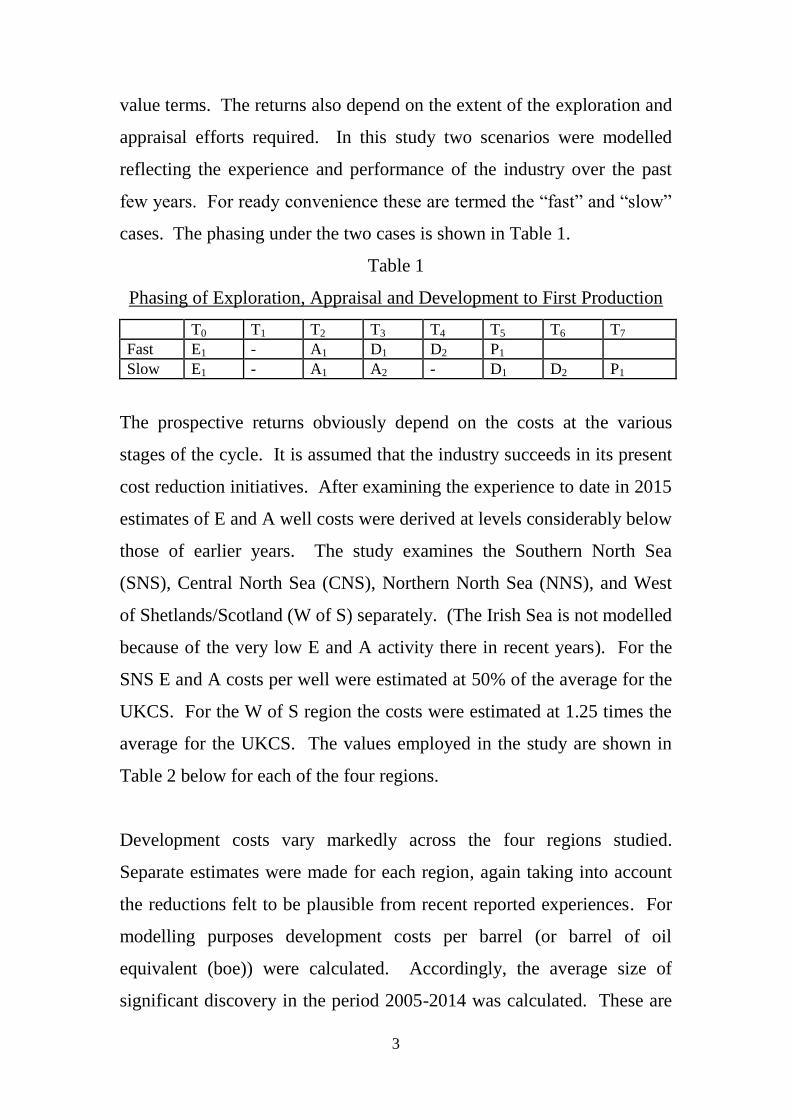
value terms. The returns also depend on the extent of the exploration and
appraisal efforts required. In this study two scenarios were modelled
reflecting the experience and performance of the industry over the past
few years. For ready convenience these are termed the “fast” and “slow”
cases. The phasing under the two cases is shown in Table 1.
Table 1
Phasing of Exploration, Appraisal and Development to First Production
T0 T1 T2 T3 T4 T5 T6 T7
Fast E1 - A1 D1 D2 P1
Slow E1 - A1 A2 - D1 D2 P1
The prospective returns obviously depend on the costs at the various
stages of the cycle. It is assumed that the industry succeeds in its present
cost reduction initiatives. After examining the experience to date in 2015
estimates of E and A well costs were derived at levels considerably below
those of earlier years. The study examines the Southern North Sea
(SNS), Central North Sea (CNS), Northern North Sea (NNS), and West
of Shetlands/Scotland (W of S) separately. (The Irish Sea is not modelled
because of the very low E and A activity there in recent years). For the
SNS E and A costs per well were estimated at 50% of the average for the
UKCS. For the W of S region the costs were estimated at 1.25 times the
average for the UKCS. The values employed in the study are shown in
Table 2 below for each of the four regions.
Development costs vary markedly across the four regions studied.
Separate estimates were made for each region, again taking into account
the reductions felt to be plausible from recent reported experiences. For
modelling purposes development costs per barrel (or barrel of oil
equivalent (boe)) were calculated. Accordingly, the average size of
significant discovery in the period 2005-2014 was calculated. These are

4
16.4 million boe for the SNS, 39.1 million boe for the CNS, 16.5 million
boe for the NNS, and 112.6 million for the W of S. The average
development costs per boe after cost reductions were then found to be
$11.39 for the SNS, $23.67 for the CNS, $17.15 for the NNS, and $11.52
for W of S. The absolute costs for W of S are higher than elsewhere but
the larger volumes pull down the relative unit costs. Development costs
were phased over 2 to 5 years depending on the size of discovery.
Annual operating costs were modelled as a percentage of accumulated
development costs with the percentage increasing as the size of field
decreased, reflecting economies of scale.
The above figures are average costs and average field sizes. This study
employs the Monte Carlo technique to reflect the uncertainties facing the
explorationist and field developer. The average values noted above were
made part of distributions of the stochastic variables which determine the
range of returns facing the explorationist. The details of the input
distributions obviously vary across each of the four regions, but have
some common features. Thus the distribution of field sizes is taken to be
lognormal with a standard deviation expressed as 50% of the mean. The
distribution of development costs per boe is taken to be normal with a
common standard deviation of 20% as a percentage of the mean value.
The mean oil price was set at $55 per barrel in real terms with the
assumption that it follows a mean-reverting behaviour through time. The
standard deviation was set at 20% of the mean. (Minimum and maximum
values from the modelling were $11 per barrel and $99 per barrel
respectively in real terms). The mean gas price was set at 40 pence per
therm in real terms with a standard deviation of 10% of the mean. Mean-
reverting behaviour is assumed. (The minimum value from the modelling
was 24 pence and the maximum 56 pence, both in real terms).

5
Other modelling assumptions relate to exploration and appraisal success
rates. Significant discoveries are defined as all those published by DECC
plus others known to the authors covering the period 2008-2014
inclusive. Appraisal success covers all fields for which development has
been started, firmly planned, or contemplated. This definition excludes
discoveries for which no field development plan is currently
contemplated.
Details of the modelling assumptions for the four regions are summarised
below in Table 2. All financial values are in real terms.

6
Table 2
Assumptions for Monte Carlo modelling by region
After Cost Reductions
Central
North Sea
Southern
North Sea
Northern
North Sea
West of
Shetlands
Exploration success 34.2% 35.3% 40% 50%
Chance of oil 82% 0% 88% 75%
Chance of gas 18% 100% 12% 25%
Appraisal success 47.4% 30% 50% 55.6%
Reserves
Average 39.1 mmboe 16.4 mmboe 16.5 mmboe 112.6 mmboe
Minimum
significant
size
8.5 mmboe 3.55 mmboe 3.6 mmboe 24.4 mmboe
Maximum
significant
size
110 mmboe 50 mmboe 50 mmboe 320 mmboe
Well costs for E & A £24.68m. £14.1m. £24.68m. £30.85m.
Average devex per
boe
$23.67 $11.392 $17.152 $15.82
Minimum devex per
boe
$9.47 $4.56 $6.86 $6.33
Maximum devex per
boe
$37.88 $18.23 $27.44 $25.32
The taxation system incorporated in the modelling reflects the changes
instigated in 2015 including the investment allowance of 62.5% for
Supplementary Charge (SC), and the reduction in the rate of SC to 20%.
The effects of several further tax incentives are modelled. These are (1)
the granting of eligibility of unsuccessful exploration costs for the
investment allowance for Supplementary Charge, (2) a refundable tax
credit for exploration to be paid to an investor who has no other current
income against which to set his allowances, (3) the ability to offset the
investment allowance against income other than that to which the new
investment relates, and (4) the award of interest (as for the Ring Fence
Expenditure Supplement) when the investment allowance, though eligible
to be activated, cannot in practice be used because the income available
7
to the investor is insufficient to absorb the allowance. Two scenarios
regarding the tax position of the investor are modelled. The first assumes
that the investor is in an ongoing tax-paying position and is able to obtain
tax relief on his exploration, appraisal and development expenditures
against income from other fields. The second scenario assumes that the
investor has no other income against which he can relieve his costs and so
utilises the Ring Fence Expenditure Supplement (RFES) to obtain later
relief against income from a future discovery. The RFES is assumed not
to apply to the IA in the modelling.
3. Results
A. Investment Allowance Eligible for All Exploration Costs
(a) Investor in Tax-Paying Position, Fast Cycle Time
i. CNS
The distribution of EMVs at 10% after the cost reductions for an
investor in a tax-paying position and with the fast cycle time
assumptions in the CNS is shown in Chart 1 (pre-tax) and Chart 2
(post-tax). There is a very wide range of outcomes, namely from ‒
£104.24 million to +£124.33 million before tax, and ‒£40.15
million to +£86.12 million after tax. There is more than a 42%
chance that the pre-tax EMV will be positive, and a 20% chance
that it will exceed +£12.55 million. 68% of the pre-tax EMV
distribution lies in the range -£21.76m. to +£15.63m. and 95% of
the distribution lies in the range -£45.01m. to +£52.61m.. After tax
there is a 37% chance that the EMV will be negative. There is a
30% chance that it will exceed +£8 million, and a 10% chance that
it will exceed +£17.61 million. 68% of the post-tax EMV
distribution lies in the range -£5.79m. to +£13.55m. and 95% of the
distribution lies in the range -£16.99m. to +£34.62m.

8
In sum the prospect facing the investor is a negative but very small
pre-tax mean expected EMV, a substantial chance of a loss, and
very limited upside potential.
Chart 1
Chart 2
CNS - Ongoing (Fast) - Initial Price $55 p/b and 40p/therm Cost Reduction
Pre-Tax EMV@10% Statistics
Trials 1000
Mean -2.40
Median -3.43
Standard Deviation 23.42
Variance 548.64
Skewness 0.62
Kurtosis 3.27
Coefficient of Variability -9.74
Minimum -104.24
Maximum 124.33
Range 228.57
Mean Standard Error 0.74
Trimmed Mean (98%) -2.61
0.00
0.01
0.02
0.03
0.04
0.05
0.06
0.07
Pro
bab
ilit
yPre-Tax EMV @ 10% - CNS
Post-Tax EMV@10% Statistics
Trials 1000
Mean 4.03
Median 2.78
Standard Deviation 12.26
Variance 150.41
Skewness 1.13
Kurtosis 4.67
Coefficient of Variability 3.04
Minimum -40.15
Maximum 86.12
Range 126.27
Mean Standard Error 0.39
Trimmed Mean (98%) 3.82
0.00
0.01
0.02
0.03
0.04
0.05
0.06
0.07
Pro
bab
ilit
y
Post-Tax EMV @ 10% - CNS
(£m)
(£m)

9
i. NNS
In Charts 3 and 4 the prospective EMVs for the investor in the
NNS after the cost reductions are shown before and after tax
respectively. The mean values are just positive in both situations.
There is a wide range of possible outcomes from a minimum of ‒
£21.76 million to +£117.43 million before tax. There is a 66%
chance that the EMV will be positive before tax, and a 20% chance
that it will exceed +£15.07 million. 68% of the pre-tax EMV
distribution lies in the range -£4.78m. to +£17.68m. and 95% of the
distribution lies in the range -£11.58m. to +£41.6m. After tax there
is an 81% chance that the EMV will be positive, and a 20% chance
that it will exceed +£10.65 million. 68% of the post-tax EMV
distribution lies in the range -£0.26m. to +£12.1m. and 95% of the
distribution lies in the range -£3.16m. to +£24.23m.
In sum the prospect facing the investor is a positive but small mean
expected EMV, a modest chance of a loss, and modest upside
potential.

10
Chart 3
Chart 4
NNS - Ongoing (Fast) - Initial Price $55 p/b and 40p/therm Cost Reduction
Pre-Tax EMV@10% Statistics
Trials 1000
Mean 6.68
Median 4.45
Standard Deviation 13.49
Variance 182.03
Skewness 1.81
Kurtosis 7.35
Coefficient of Variability 2.02
Minimum -21.76
Maximum 117.43
Range 139.18
Mean Standard Error 0.43
Trimmed Mean (98%) 6.30
0.00
0.01
0.02
0.03
0.04
0.05
0.06
0.07
Pro
bab
ilit
y
Pre-Tax EMV @ 10% - NNS
Post-Tax EMV@10% Statistics
Trials 1000
Mean 6.12
Median 4.90
Standard Deviation 7.31
Variance 53.49
Skewness 2.01
Kurtosis 9.17
Coefficient of Variability 1.19
Minimum -7.18
Maximum 71.16
Range 78.34
Mean Standard Error 0.23
Trimmed Mean (98%) 5.89
0.00
0.01
0.02
0.03
0.04
0.05
0.06
0.07
Pro
bab
ilit
y
Post-Tax EMV @ 10% - NNS
(£m)
(£m)

11
ii. SNS
The distributions of EMVs for the investor in the SNS after cost
reductions are shown in Chart 5 (pre-tax) and Chart 6 (post-tax).
There is only a 5% chance that the pre-tax EMV will be negative,
and a 20% chance that it will be more than +£7.96 million. 68% of
the pre-tax EMV distribution lies in the range +£1.26m. to
+£8.98m. and 95% of the distribution lies in the range -£0.58m. to
+£16.36m. After tax there is only 1% chance that the EMV will be
negative. However, there is only a 10% chance that the value will
exceed +£6.6 million. 68% of the post-tax EMV distribution lies
in the range +£1.39m. to +£5.56m. and 95% of the distribution lies
in the range +£0.29m. to +£9.57m.
In sum the prospect facing the investor is a positive but modest
mean expected EMV, a very low chance of a loss, and very limited
upside potential.

12
Chart 5
Chart 6
SNS - Ongoing (Fast) - Initial Price $55 p/b and 40p/therm Cost Reduction
Pre-Tax EMV@10% Statistics
Trials 1000
Mean 5.13
Median 4.22
Standard Deviation 4.36
Variance 19.00
Skewness 1.46
Kurtosis 3.30
Coefficient of Variability 0.85
Minimum -2.30
Maximum 30.65
Range 32.95
Mean Standard Error 0.14
Trimmed Mean (98%) 5.01
0.00
0.01
0.02
0.03
0.04
0.05
0.06
0.07
Pro
bab
ilit
y
Pre-Tax EMV @ 10% - SNS
Post-Tax EMV@10% Statistics
Trials 1000
Mean 3.52
Median 3.10
Standard Deviation 2.43
Variance 5.91
Skewness 1.44
Kurtosis 3.31
Coefficient of Variability 0.69
Minimum -0.44
Maximum 17.95
Range 18.39
Mean Standard Error 0.08
Trimmed Mean (98%) 3.46
0.00
0.01
0.02
0.03
0.04
0.05
0.06
0.07
Pro
bab
ilit
y
Post-Tax EMV @ 10% - SNS
(£m)
(£m)

13
iii. W of S
The distributions of EMVs for the investor in the W of S region
after cost reductions are shown in Chart 7 (pre-tax) and Chart 8
(post-tax). It is seen that the mean values are substantially positive
both before and after tax for the investor already in a tax-paying
position. However, the spread of outcomes is extremely wide with
a pre-tax minimum value of ‒£153.91 million and a maximum of
+£1042.31 million. There is a 10% chance that the EMV will be
negative and a 20% chance that it will exceed +£212.29 million
before tax. 68% of the pre-tax EMV distribution lies in the range
+£16.09m. to +£237.27m. and 95% of the distribution lies in the
range -£54.63m. to +£452.22m. After tax the chance that the EMV
will be negative is less than 5%, and there is a 20% chance that it
will exceed +£127.58 million. 68% of the post-tax EMV
distribution lies in the range +£21.97m. to +£140.44m. and 95% of
the distribution lies in the range -£7.83m. to +£264.01m.
In sum the prospect facing the investor is a substantial positive
mean expected EMV, a modest chance of a loss, and large upside
potential. But investment costs are very high in this region.

14
Chart 7
Chart 8
(b) Project Investor, Fast Cycle Time
i. CNS
The distribution of EMVs for the project investor after cost
reductions is shown in Chart 9 (post-tax). Of course, pre-tax is as
WoS - Ongoing (Fast) - Initial Price $55 p/b and 40p/therm Cost Reduction
Pre-Tax EMV@10% Statistics
Trials 1000
Mean 126.46
Median 101.08
Standard Deviation 126.47
Variance 15994.12
Skewness 1.40
Kurtosis 4.14
Coefficient of Variability 1.00
Minimum -153.91
Maximum 1042.31
Range 1196.21
Mean Standard Error 4.00
Trimmed Mean (98%) 123.63
0.00
0.01
0.02
0.03
0.04
0.05
0.06
Pro
bab
ilit
y
Pre-Tax EMV @ 10% - WoS
Post-Tax EMV@10% Statistics
Trials 1000
Mean 81.17
Median 65.61
Standard Deviation 67.88
Variance 4607.26
Skewness 1.55
Kurtosis 4.87
Coefficient of Variability 0.84
Minimum -48.77
Maximum 604.11
Range 652.89
Mean Standard Error 2.15
Trimmed Mean (98%) 79.45
0.00
0.01
0.02
0.03
0.04
0.05
0.06
0.07
Pro
bab
ilit
y
Post-Tax EMV @ 10% - WoS
(£m)
(£m)

15
for the ongoing investor with cost reductions. The mean value is
negative at -£4.58 million after tax. After tax the chance of a
negative EMV is 59%, but there is a 30% chance that it will be
greater than +£3.86 million. 68% of the post-tax EMV distribution
lies in the range -£20.59m. to +£10.17m. and 95% of the
distribution lies in the range -£43.24m. to +£30.79m.
With a deterministic system where all variables are as the mean
values, the project investor with an oil find can write off his costs
and take advantage of the RFES but he can only use 28% of the IA
to which he is entitled. The project investor with a gas find can
write off his costs but can only take advantage of 34% of the
RFES and none of the IA to which he is entitled.
Chart 9
In sum the prospect facing the investor is a negative mean expected
EMV, a high chance of a loss, and modest upside potential.
CNS - Project (Fast) - Initial Price $55 p/b and 40p/therm Cost Reduction
Post-Tax EMV@10% Statistics
Trials 1000
Mean -4.58
Median -3.07
Standard Deviation 18.32
Variance 335.64
Skewness -0.36
Kurtosis 2.56
Coefficient of Variability -4.00
Minimum -102.31
Maximum 73.01
Range 175.33
Mean Standard Error 0.58
Trimmed Mean (98%) -4.48
0.00
0.01
0.02
0.03
0.04
0.05
0.06
Pro
bab
ilit
y
Post-Tax EMV @ 10% - CNS (£m)

16
ii. NNS
In the NNS the distribution of EMVs for the project investor is
shown in Chart 10 (post-tax). The mean value is positive to a
modest degree. After tax the chance of the EMV being negative is
just over 33%, but there is a 20% chance that it will exceed
+£10.18 million. 68% of the post-tax EMV distribution lies in the
range -£4.4m. to +£11.76m. and 95% of the distribution lies in the
range -£10.9m. to +£24.72m.
With a deterministic system where all variables are as the mean
values, the project investor with an oil find can write off his costs
and take advantage of the RFES, but he can only use 70% of the IA
to which he is entitled. The project investor with a gas find can
write off his costs but can only take advantage of 65% of the
RFES, and he cannot use any of the IA to which he is entitled.
Chart 10
In sum the prospect facing the investor is a positive but small mean
expected EMV, a significant chance of a loss, and modest upside
potential.
NNS - Project (Fast) - Initial Price $55 p/b and 40p/therm Cost ReductionPost-Tax EMV@10% Statistics
Trials 1000
Mean 4.02
Median 3.63
Standard Deviation 8.98
Variance 80.67
Skewness 0.96
Kurtosis 3.82
Coefficient of Variability 2.23
Minimum -20.92
Maximum 68.21
Range 89.12
Mean Standard Error 0.28
Trimmed Mean (98%) 3.86
0.00
0.01
0.02
0.03
0.04
0.05
0.06
Pro
bab
ilit
y
Post-Tax EMV @ 10% - NNS (£m)

17
iii. SNS
The distribution of EMVs at 10% for the project investor in the
SNS is shown in Chart 11 (post-tax). The mean values are just
negative before and after tax. After tax the chance of a negative
EMV is 4%, and there is only a 10% chance of the value exceeding
+£6.56 million. 68% of the post-tax EMV distribution lies in the
range +£1.12m. to +£5.64m. and 95% of the distribution lies in the
range -£0.51m. to +£9.72m.
With a deterministic system where all variables are as the mean
values, the project investor can write off his costs, take advantage
of the RFES and use 100% of the IA to which he is entitled.
Chart 11
In sum the prospect facing the investor is a positive but small mean
expected EMV, a very low chance of a loss, and very small upside
potential.
SNS - Project (Fast) - Initial Price $55 p/b and 40p/therm Cost Reduction
Post-Tax EMV@10% Statistics
Trials 1000
Mean 3.44
Median 3.11
Standard Deviation 2.53
Variance 6.39
Skewness 1.09
Kurtosis 2.34
Coefficient of Variability 0.74
Minimum -2.16
Maximum 17.52
Range 19.68
Mean Standard Error 0.08
Trimmed Mean (98%) 3.38
0.000
0.005
0.010
0.015
0.020
0.025
0.030
0.035
0.040
0.045
0.050
Pro
bab
ilit
y
Post-Tax EMV @ 10% - SNS (£m)

18
iv. W of S
The distribution of EMVs for the project investor in the W of S
region is shown in Chart 12 (post-tax). The mean value is healthily
positive at £71.82 million after tax. After tax there is an 11%
chance that the EMV will be negative, a 30% chance that it will
exceed +£97.02 million, and a 10% chance that it will exceed
+£163.61 million. 68% of the post-tax EMV distribution lies in
the range +£10.11m. to +£134.73m., and 95% of the distribution
lies in the range -£52.24m. to +£253.67m.
With a deterministic system where all variables are as the mean
values, the project investor with an oil find can write off his costs,
take advantage of the RFES and use 100% of the IA to which he is
entitled. The project investor with a gas find can write off his costs
but can only take advantage of 68% of the RFES, and he cannot
use any of the IA to which he is entitled.

19
Chart 12
In sum the prospect facing the investor is a substantial mean
expected EMV, a modest chance of a loss, and large upside
potential. But the investment costs are very high.
B. Tax Credit for Exploration
(a) Project Investor, Fast Cycle Time
i. CNS
The distribution of EMVs at 10% to an investor who has no tax
capacity at the time of the investment and receives an exploration
tax credit is shown in Chart 13 (post-tax). (The pre-tax is, of
course unchanged). After tax the spread is from ‒£100.32 million
to +£73.16 million. There is a greater than 56% chance that the
EMV will be negative, and a 30% chance that the value will be ‒
£10.09 million or worse. There is just over a 17% chance that the
EMV will exceed +£10 million. 68% of the post-tax EMV
distribution lies in the range -£18.59m. to +£10.11m., and 95% of
the distribution lies in the range -£41.25m. to +£30.52m.
WoS - Project (Fast) - Initial Price $55 p/b and 40p/therm Cost ReductionPost-Tax EMV@10% Statistics
Trials 1000
Mean 71.82
Median 60.26
Standard Deviation 73.05
Variance 5336.22
Skewness 1.02
Kurtosis 3.26
Coefficient of Variability 1.02
Minimum -149.83
Maximum 571.94
Range 721.77
Mean Standard Error 2.31
Trimmed Mean (98%) 70.79
0.00
0.01
0.02
0.03
0.04
0.05
0.06
Pro
bab
ilit
y
Post-Tax EMV @ 10% - WoS (£m)

20
With a deterministic system, where all variables are as the mean
values, with a tax credit, the project investor with an oil find can
write off his costs and take advantage of the RFES (which is
reduced with the credit), but he can only use 42% of the IA to
which he is entitled. The project investor with a gas find and tax
credit can write off his costs but can only take advantage of 47% of
the (reduced) RFES and he cannot use any of the IA to which he is
entitled.
In sum the prospect facing the investor is a negative mean expected
EMV, a high chance of a loss, and limited upside potential.
Chart 13
ii. NNS
The distribution of EMVs at 10% to a project investor in the NNS
with the tax credit and reduced costs is shown in Chart 14 (post-
CNS - Project (Fast) Tax Credit - Initial Price $55 p/b and 40p/therm Reduced Costs
Post-Tax EMV@10% Statistics
Trials 1000
Mean -3.51
Median -1.89
Standard Deviation 17.61
Variance 309.94
Skewness -0.42
Kurtosis 2.98
Coefficient of Variability -5.02
Minimum -100.32
Maximum 73.16
Range 173.47
Mean Standard Error 0.56
Trimmed Mean (98%) -3.40
0.00
0.01
0.02
0.03
0.04
0.05
0.06
0.07
Pro
bab
ilit
y
Post-Tax EMV @ 10% - CNS (£m)

21
tax). The chance of a negative EMV is 26%, but there is only a
10% chance that the value could be +£14.05 million or better. 68%
of the post-tax EMV distribution lies in the range -£2.17m. to
+£11.25m., and 95% of the distribution lies in the range -£8.43m.
to +£23.87m.
With a deterministic system where all variables are as the mean
values and a tax credit, the project investor with an oil discovery
can write off his costs and take advantage of the RFES (which is
reduced with the credit) and use all of the IA to which he is
entitled. The project investor with a gas find and a tax credit can
write off his costs and take advantage of the (reduced) RFES, but
he can only use 12% of the IA to which he is entitled.
In sum the prospect facing the investor is a positive but small mean
expected EMV, significant chance of a loss, and modest upside
potential.

22
Chart 14
iii. SNS
The distribution of EMVs to a project investor in the SNS with a
tax credit and reduced costs is shown in Chart 15 (post-tax). In this
case the chance of a negative EMV is only 3% after tax. 68% of
the post-tax EMV distribution lies in the range +£1.21m. to
+£5.41m., and 95% of the distribution lies in the range -£0.04m. to
+£9.52m. These are very modest values.
With a deterministic system where all variables are as the mean
values with the tax credit the project investor can write off his
costs, take advantage of the (reduced) RFES and use 100% of the
IA to which he is entitled.
In sum the prospect facing the investor is a positive but very small
mean expected EMV, a low chance of a loss, and very limited
upside potential.
NNS - Project (Fast) Tax Credit - Initial Price $55 p/b and 40p/therm Reduced Costs
Post-Tax EMV@10% Statistics
Trials 1000
Mean 4.67
Median 3.93
Standard Deviation 8.09
Variance 65.49
Skewness 1.29
Kurtosis 5.65
Coefficient of Variability 1.73
Minimum -18.45
Maximum 67.82
Range 86.27
Mean Standard Error 0.26
Trimmed Mean (98%) 4.51
0.00
0.01
0.02
0.03
0.04
0.05
0.06
0.07
Pro
bab
ilit
y
Post-Tax EMV @ 10% - NNS (£m)

23
Chart 15
iv. W of S
The distribution of EMVs for a project investor in the W of S
region with the tax credit and reduced costs is shown in Chart 16
(post-tax). There is a 10% chance that the EMV will be negative.
There is a 20% chance that the EMV could be +£121.65 million or
better, and a 10% chance that it could be +£163.22 million or
better. 68% of the post-tax EMV distribution lies in the range
+£11.15m. to +£134.27m., and 95% of the distribution lies in the
range -£47.96m. to +£249.25m.
With a deterministic system where all variables are as the mean
values, the project investor with an oil find and a tax credit for
exploration can write off his costs, take advantage of the RFES,
and use 100% of the IA to which he is entitled. The project
investor with a gas find and a tax credit can write off his costs and
take advantage of the (reduced) RFES, but he can only use 79% of
the IA to which he is entitled.
SNS - Project (Fast) Tax Credit - Initial Price $55 p/b and 40p/therm Reduced Costs
Post-Tax EMV@10% Statistics
Trials 1000
Mean 3.38
Median 2.99
Standard Deviation 2.40
Variance 5.77
Skewness 1.30
Kurtosis 2.93
Coefficient of Variability 0.71
Minimum -1.41
Maximum 17.36
Range 18.77
Mean Standard Error 0.08
Trimmed Mean (98%) 3.32
0.00
0.01
0.02
0.03
0.04
0.05
0.06
Pro
bab
ilit
y
Post-Tax EMV @ 10% - SNS (£m)

24
In sum the prospect facing the investor is a substantial mean
expected EMV, modest chance of a loss, and high upside potential.
But investment costs are also very high.
Chart 16
C. Investment Allowance Limited to Successful Exploration
(a) Investor in Tax-Paying Position, Fast Cycle Time
i. CNS
In Chart 17 the post-tax EMVs at 10% real discount rate is shown
when the IA for exploration is limited by the exploration success
rate and costs are reduced. This is the current tax position. The
chance of a negative post-tax EMV is 38%. There is only a 7%
chance that the EMV will exceed +£20 million after tax. 68% of
the post-tax EMV distribution lies in the range -£5.87m. to
+£13.43m., and 95% of the distribution lies in the range -£16.99m.
to +£34.51m.
WoS - Project (Fast) Tax Credit - Initial Price $55 p/b and 40p/therm Reduced Costs
Post-Tax EMV@10% Statistics
Trials 1000
Mean 71.92
Median 59.84
Standard Deviation 72.11
Variance 5200.51
Skewness 1.08
Kurtosis 3.42
Coefficient of Variability 1.00
Minimum -145.54
Maximum 571.36
Range 716.90
Mean Standard Error 2.28
Trimmed Mean (98%) 70.86
0.00
0.01
0.02
0.03
0.04
0.05
0.06
0.07P
rob
ab
ilit
y
Post-Tax EMV @ 10% - WoS (£m)

25
In sum, the prospect facing the investor is a positive but small
mean expected EMV, a substantial risk of a loss, and modest
upside potential.
Chart 17
ii. NNS
When the key risks are included, the IA for exploration is
restricted, and costs are reduced, the distribution of EMVs at 10%
is shown in Chart 18 (post-tax). There is a 19% chance that the
EMV will be negative. 68% of the post-tax EMV distribution lies
in the range -£0.4m. to +£11.94m., and 95% of the distribution lies
in the range -£3.27m. to +£24.07m.
In sum, the prospect facing the investor is a positive but small
mean expected EMV, a modest chance of a loss, and modest upside
potential.
CNS - Ongoing (Fast) Limited IA - Initial Price $55 p/b and 40p/therm Reduced Costs
Post-Tax EMV@10% Statistics
Trials 1000
Mean 3.95
Median 2.69
Standard Deviation 12.24
Variance 149.72
Skewness 1.14
Kurtosis 4.71
Coefficient of Variability 3.10
Minimum -40.15
Maximum 86.02
Range 126.17
Mean Standard Error 0.39
Trimmed Mean (98%) 3.74
0.00
0.01
0.02
0.03
0.04
0.05
0.06
0.07
Pro
bab
ilit
y
Post-Tax EMV @ 10% - CNS (£m)

26
Chart 18
iii. SNS
When the key risks are considered, the IA for exploration is
restricted, and costs are reduced, the post-tax distribution of EMVs
is shown in Chart 19. The chance of a negative EMV is only 1%.
68% of the post-tax EMV distribution lies in the range +£1.33m. to
+£5.51m., and 95% of the distribution lies in the range +£0.24m. to
+£9.52m.
In sum, the prospect facing the investor is for a positive but modest
mean expected EMV, a very small chance of a loss, and very
limited upside potential.
NNS - Ongoing (Fast) Limited IA - Initial Price $55 p/b and 40p/therm Reduced Costs
Post-Tax EMV@10% Statistics
Trials 1000
Mean 5.98
Median 4.75
Standard Deviation 7.31
Variance 53.39
Skewness 2.02
Kurtosis 9.21
Coefficient of Variability 1.22
Minimum -7.26
Maximum 71.02
Range 78.28
Mean Standard Error 0.23
Trimmed Mean (98%) 5.74
0.00
0.01
0.02
0.03
0.04
0.05
0.06
0.07
Pro
bab
ilit
y
Post-Tax EMV @ 10% - NNS (£m)

27
Chart 19
iv. W of S
When the key risks are taken into account, the IA for exploration is
restricted, and costs are reduced, the post-tax distribution of EMVs
at 10% is shown in Chart 20. The chance of a negative EMV is
4%. There is a 30% chance that the EMV could exceed +£100
million. 68% of the post-tax EMV distribution lies in the range
+£21.81m. to +£140.25m., and 95% of the distribution lies in the
range -£7.95m. to +£263.8m.
In sum, the prospect facing the investor is a large mean expected
EMV, small chance of a loss, and substantial upside potential. But
investment costs are very high.
SNS - Ongoing (Fast) Limited IA - Initial Price $55 p/b and 40p/therm Reduced Costs
Post-Tax EMV@10% Statistics
Trials 1000
Mean 3.47
Median 3.04
Standard Deviation 2.43
Variance 5.92
Skewness 1.44
Kurtosis 3.31
Coefficient of Variability 0.70
Minimum -0.49
Maximum 17.90
Range 18.39
Mean Standard Error 0.08
Trimmed Mean (98%) 3.41
0.00
0.01
0.02
0.03
0.04
0.05
0.06
Pro
bab
ilit
y
Post-Tax EMV @ 10% - SNS (£m)

28
Chart 20
(b) Project Investor, Fast Cycle Time
i. CNS
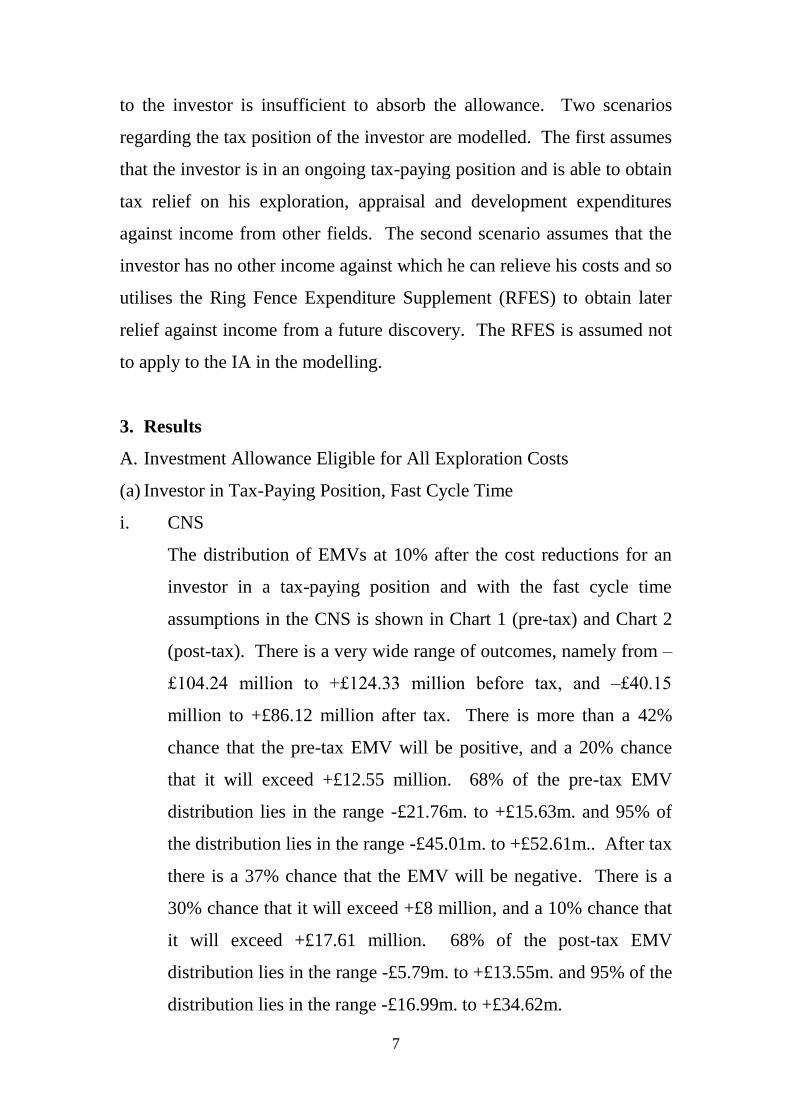
The distribution of EMVs at 10% to an investor who has no tax
capacity at the time of the investment, restricted IA for exploration,
and reduced costs is shown in Chart 21 (post-tax). The spread is
from ‒£102.31 million to +£72.96 million. There is a more than
58% chance that the EMV will be negative, with a 30% chance that
the value will be ‒£11.99 million or worse. There is only a 16%
chance that the EMV will exceed +£10 million. 68% of the post-
tax EMV distribution lies in the range -£20.59m. to +£10.1m., and
95% of the distribution lies in the range -£43.24m. to +£30.69m.
With a deterministic system where all variables are as the mean
values with limited IA the project investor with an oil find can
write off his costs and take advantage of the RFES, but he can only
use 29% of the IA to which he is entitled. The project investor
with a gas find can write off his costs, but can only take advantage
WoS - Ongoing (Fast) Limited IA - Initial Price $55 p/b and 40p/therm Reduced Costs
Post-Tax EMV@10% Statistics
Trials 1000
Mean 80.99
Median 65.41
Standard Deviation 67.86
Variance 4604.78
Skewness 1.56
Kurtosis 4.88
Coefficient of Variability 0.84
Minimum -48.85
Maximum 603.95
Range 652.80
Mean Standard Error 2.15
Trimmed Mean (98%) 79.27
0.00
0.01
0.02
0.03
0.04
0.05
0.06
0.07
Pro
bab
ilit
y
Post-Tax EMV @ 10% - WoS (£m)
29
of 34% of the RFES, and he cannot use any of the IA to which he
is entitled.
In sum the prospect facing the investor is a small negative mean
expected EMV, large chance of a loss, and limited upside potential
Chart 21
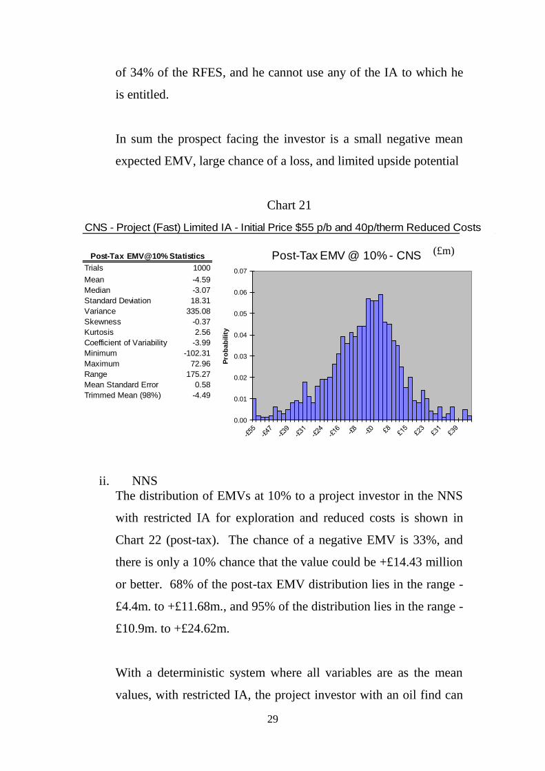
ii. NNS
The distribution of EMVs at 10% to a project investor in the NNS
with restricted IA for exploration and reduced costs is shown in
Chart 22 (post-tax). The chance of a negative EMV is 33%, and
there is only a 10% chance that the value could be +£14.43 million
or better. 68% of the post-tax EMV distribution lies in the range -
£4.4m. to +£11.68m., and 95% of the distribution lies in the range -
£10.9m. to +£24.62m.
With a deterministic system where all variables are as the mean
values, with restricted IA, the project investor with an oil find can
CNS - Project (Fast) Limited IA - Initial Price $55 p/b and 40p/therm Reduced Costs
Post-Tax EMV@10% Statistics
Trials 1000
Mean -4.59
Median -3.07
Standard Deviation 18.31
Variance 335.08
Skewness -0.37
Kurtosis 2.56
Coefficient of Variability -3.99
Minimum -102.31
Maximum 72.96
Range 175.27
Mean Standard Error 0.58
Trimmed Mean (98%) -4.49
0.00
0.01
0.02
0.03
0.04
0.05
0.06
0.07
Pro
bab
ilit
y
Post-Tax EMV @ 10% - CNS (£m)

30
write off his costs and take advantage of the RFES, but he can only
use a 75% of the IA to which he is entitled. The project investor
with a gas find can write off his costs and take advantage of 65%
of the RFES, but he cannot use any of the IA to which he is
entitled.
In sum the prospect facing the investor is a positive but small mean
expected EMV, substantial risk of a loss, and limited upside
potential.
Chart 22
iii. SNS
The distribution of EMVs to a project investor in the SNS with
restricted IA for exploration and reduced costs is shown in Chart
23 (post-tax). The chance of a negative EMV is only 4%. 68% of
the post-tax EMV distribution lies in the range +£1.12m. to
+£5.6m., and 95% of the distribution lies in the range -£0.51m. to
+£9.68m.
NNS - Project (Fast) Limited IA - Initial Price $55 p/b and 40p/therm Reduced Costs
Post-Tax EMV@10% Statistics
Trials 1000
Mean 3.99
Median 3.63
Standard Deviation 8.95
Variance 80.10
Skewness 0.96
Kurtosis 3.84
Coefficient of Variability 2.24
Minimum -20.92
Maximum 68.09
Range 89.01
Mean Standard Error 0.28
Trimmed Mean (98%) 3.84
0.00
0.01
0.02
0.03
0.04
0.05
0.06
Pro
bab
ilit
y
Post-Tax EMV @ 10% - NNS (£m)

31
With a deterministic system where all variables are as the mean
values the project investor can write off his costs, take advantage
of the RFES, and use 100% of the IA to which he is entitled.
In sum, the prospect facing the investor is a positive but small
mean expected EMV, low chance of a loss, and very limited upside
potential.
Chart 23
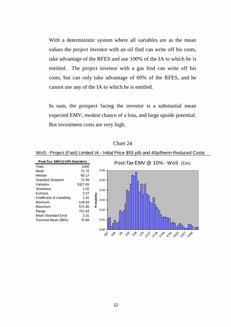
iv. W of S
The distribution of EMVs for a project investor in the W of S
region with restricted IA for exploration and reduced costs is
shown in Chart 24 (post-tax). There is an 11% chance that the
EMV will be negative, and a 20% chance that the value could be
+£17.31 million or worse. There is a 10% chance that the EMV
could +£163.45 million or better. 68% of the post-tax EMV
distribution lies in the range +£10.11m. to +£134.64m., and 95% of
the distribution lies in the range -£52.24m. to +£253.51m.
SNS - Project (Fast) Limited IA - Initial Price $55 p/b and 40p/therm Reduced Costs
Post-Tax EMV@10% Statistics
Trials 1000
Mean 3.42
Median 3.10
Standard Deviation 2.51
Variance 6.32
Skewness 1.10
Kurtosis 2.39
Coefficient of Variability 0.73
Minimum -2.16
Maximum 17.48
Range 19.64
Mean Standard Error 0.08
Trimmed Mean (98%) 3.37
0.00
0.01
0.02
0.03
0.04
0.05
0.06
Pro
bab
ilit
y
Post-Tax EMV @ 10% - SNS (£m)
32
With a deterministic system where all variables are as the mean
values the project investor with an oil find can write off his costs,
take advantage of the RFES and use 100% of the IA to which he is
entitled. The project investor with a gas find can write off his
costs, but can only take advantage of 69% of the RFES, and he
cannot use any of the IA to which he is entitled.
In sum, the prospect facing the investor is a substantial mean
expected EMV, modest chance of a loss, and large upside potential.
But investment costs are very high.
Chart 24
WoS - Project (Fast) Limited IA - Initial Price $55 p/b and 40p/therm Reduced Costs
Post-Tax EMV@10% Statistics
Trials 1000
Mean 71.72
Median 60.17
Standard Deviation 72.99
Variance 5327.65
Skewness 1.02
Kurtosis 3.27
Coefficient of Variability 1.02
Minimum -149.83
Maximum 571.80
Range 721.63
Mean Standard Error 2.31
Trimmed Mean (98%) 70.69
0.00
0.01
0.02
0.03
0.04
0.05
0.06
Pro
bab
ilit
y
Post-Tax EMV @ 10% - WoS (£m)

33
D. Immediate Relief for Investment Allowance
(a) Investor in Tax-Paying Position, Fast Cycle Time
i. CNS
In Chart 25 the post-tax EMVs at 10% real discount rate with
immediate relief for IA and reduced costs are shown. The chance
of a negative post-tax EMV is 24%. There is a 10% chance that
the EMV will exceed +£20 million. 68% of the post-tax EMV
distribution lies in the range -£2.07m. to +£16.51m., and 95% of
the distribution lies in the range -£8.99m. to +£36.84m.
In sum the prospect facing the investor is a positive but small mean
expected EMV, significant downside risks, and modest upside
potential.
Chart 25
ii. NNS
When the key risks are included and there is immediate relief for
IA and reduced costs the distribution of EMVs at 10% is shown in
Chart 26 (post-tax) for the explorer in the NNS. There is an 8%
CNS - Ongoing (Fast Tax Saved) - Initial Price $55 p/b and 40p/therm Cost Reduction
Post-Tax EMV@10% Statistics
Trials 1000
Mean 7.36
Median 5.55
Standard Deviation 11.59
Variance 134.38
Skewness 1.75
Kurtosis 7.17
Coefficient of Variability 1.57
Minimum -23.96
Maximum 99.15
Range 123.10
Mean Standard Error 0.37
Trimmed Mean (98%) 7.06
0.00
0.01
0.02
0.03
0.04
0.05
0.06
0.07
Pro
bab
ilit
y
Post-Tax EMV @ 10% - CNS (£m)

34
chance that the EMV will be negative. 68% of the post-tax EMV
distribution lies in the range +£1.05m. to +£13.58m., and 95% of
the distribution lies in the range -£1.77m. to +£25.78m.
In sum, the mean expected post-tax EMV is positive but modest,
the downside risk is low, and the upside potential moderate.
Chart 26
iii. SNS
When the key risks are considered and relief is given for IA
immediately and costs are reduced the post-tax distribution of
EMVs is shown in Chart 27 for the explorer in the SNS. The
chance of a negative EMV is less than 1%. 68% of the post-tax
EMV distribution lies in the range +£1.73m. to +£6.11m., and 95%
of the distribution lies in the range +£0.6m. to +£10.14m.
In sum, the mean expected post-tax EMV is just positive, the
downside risk is low, and the upside potential modest.
NNS - Ongoing (Fast Tax Saved) - Initial Price $55 p/b and 40p/therm Cost Reduction
Post-Tax EMV@10% Statistics
Trials 1000
Mean 7.53
Median 6.09
Standard Deviation 7.40
Variance 54.76
Skewness 2.07
Kurtosis 9.70
Coefficient of Variability 0.98
Minimum -4.42
Maximum 74.69
Range 79.11
Mean Standard Error 0.23
Trimmed Mean (98%) 7.28
0.00
0.01
0.02
0.03
0.04
0.05
0.06
Pro
bab
ilit
y
Post-Tax EMV @ 10% - NNS (£m)

35
Chart 27
iv. W of S
When the key risks are taken into account, relief for IA is
immediate, and costs are reduced the post-tax distribution of EMVs
at 10% is shown in Chart 28 for the explorer in W of S. The
chance of a negative EMV is less than 1%. There is a 33% chance
that the EMV could exceed +£100 million. 68% of the post-tax
EMV distribution lies in the range +£29.65m. to +£148.2m., and
95% of the distribution lies in the range +£8.45m. to +£268.59m.
In sum, the mean expected post-tax EMV is very substantially
positive, and there is a large upside potential. But the investment
costs are very large.
SNS - Ongoing (Fast Tax Saved) - Initial Price $55 p/b and 40p/therm Cost Reduction
Post-Tax EMV@10% Statistics
Trials 1000
Mean 3.96
Median 3.51
Standard Deviation 2.51
Variance 6.30
Skewness 1.42
Kurtosis 3.21
Coefficient of Variability 0.63
Minimum -0.11
Maximum 18.79
Range 18.90
Mean Standard Error 0.08
Trimmed Mean (98%) 3.89
0.00
0.01
0.02
0.03
0.04
0.05
0.06
0.07
Pro
bab
ilit
y
Post-Tax EMV @ 10% - SNS (£m)

36
Chart 28
E. Interest on Unutilised IA from time of Eligibility for Activation
(a) Project Investor, Fast Cycle Time
i. CNS
The distribution of EMVs at 10% to an investor who has no tax
capacity at the time of the investment and interest is given on
unutilised IA at the RFES rate, is shown in Chart 29 (post-tax).
There is a more than 56% chance that the EMV will be negative,
with a 30% chance that the value will be ‒£11.94 million or worse.
There is only a 24% chance that the EMV will exceed +£10
million. 68% of the post-tax EMV distribution lies in the range -
£20.59m. to +£16.58m., and 95% of the distribution lies in the
range -£43.24m. to +£53.466m.
In sum, the mean expected post-tax EMV is just negative, there is
substantial downside risk, but also substantial upside potential.
WoS - Ongoing (Fast Tax Saved) - Initial Price $55 p/b and 40p/therm Cost Reduction
Post-Tax EMV@10% Statistics
Trials 1000
Mean 89.03
Median 71.88
Standard Deviation 67.56
Variance 4563.84
Skewness 1.74
Kurtosis 6.11
Coefficient of Variability 0.76
Minimum -14.17
Maximum 648.19
Range 662.36
Mean Standard Error 2.14
Trimmed Mean (98%) 87.09
0.00
0.01
0.02
0.03
0.04
0.05
0.06
Pro
bab
ilit
y
Post-Tax EMV @ 10% - WoS (£m)

37
Chart 29
ii. NNS
The distribution of EMVs at 10% to a project investor in the NNS
when interest is given on unutilised IA and costs are reduced is
shown in Chart 30 (post-tax). The chance of a negative EMV is
35%, and there is only a 10% chance that the value could be
+£23.35 million or better. 68% of the post-tax EMV distribution
lies in the range -£4.4m. to +£18.19m., and 95% of the distribution
lies in the range -£10.9m. to +£41m.
When interest is given on unused IA, the project investor with an
oil find can write off his costs, but can only use 5% of his RFES,
and cannot use any of the IA to which he is entitled. With a gas
find and interest on unused IA the project investor can write off his
costs, but he can only use 2% of his RFES and none of the IA to
which he is entitled.
CNS - Project (Fast Interest on IA) - Initial Price $55 p/b and 40p/therm Cost Reduction
Post-Tax EMV@10% Statistics
Trials 1000
Mean -1.40
Median -2.58
Standard Deviation 23.10
Variance 533.74
Skewness 0.63
Kurtosis 3.20
Coefficient of Variability -16.54
Minimum -102.31
Maximum 126.22
Range 228.54
Mean Standard Error 0.73
Trimmed Mean (98%) -1.60
0.00
0.01
0.02
0.03
0.04
0.05
0.06
0.07
Pro
bab
ilit
y
Post-Tax EMV @ 10% - CNS (£m)

38
In sum, the mean expected post-tax EMV is modest, the downside
risks are noteworthy, and the upside potential modest.
Chart 30
iii. SNS
The distribution of EMVs to a project investor in the SNS when
interest is given on IA and costs are reduced is shown in Chart 31
(post-tax). The chance of a negative EMV is 4%. 68% of the post-
tax EMV distribution lies in the range +£1.39m. to +£9.18m., and
95% of the distribution lies in the range -£0.51m. to +£16.45m.
With interest on unused IA the project investor can write off his
costs but he can only use 6% of his RFES and none of the IA to
which he is entitled.
In sum, the post-tax expected EMV is positive but small, the
downside risks are modest, and the upside potential modest.
NNS - Project (Fast Interest on IA) - Initial Price $55 p/b and 40p/therm Cost Reduction
Post-Tax EMV@10% Statistics
Trials 1000
Mean 7.13
Median 4.93
Standard Deviation 13.39
Variance 179.25
Skewness 1.77
Kurtosis 7.28
Coefficient of Variability 1.88
Minimum -20.92
Maximum 119.30
Range 140.22
Mean Standard Error 0.42
Trimmed Mean (98%) 6.76
0.00
0.01
0.02
0.03
0.04
0.05
0.06
0.07
Pro
bab
ilit
y
Post-Tax EMV @ 10% - NNS (£m)

39
Chart 31
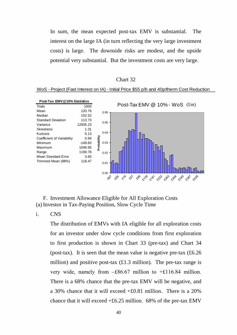
iv. W of S
The distribution of EMVs for a project investor in the W of S
region with interest on IA and reduced costs is shown in Chart 32
(post-tax). There is a 10% chance that the EMV will be negative.
There is a more than 50% chance that the EMV could be +£100
million or better, and a 10% chance that it could be +£265.93
million or better. 68% of the post-tax EMV distribution lies in the
range +£17.98m. to +£219.9m., and 95% of the distribution lies in
the range -£52.24m. to +£385.18m.
When interest is given on unused IA, the project investor with an
oil find can write off his costs, but can only use 7% of his RFES,
and 16% of the IA to which he is entitled. With a gas find and
interest on unused IA the project investor can write off his costs,
but he can only use 4% of his RFES, and none of the IA to which
he is entitled.
SNS - Project (Fast Interest on IA) - Initial Price $55 p/b and 40p/therm Cost Reduction
Post-Tax EMV@10% Statistics
Trials 1000
Mean 5.28
Median 4.39
Standard Deviation 4.36
Variance 18.99
Skewness 1.43
Kurtosis 3.19
Coefficient of Variability 0.83
Minimum -2.16
Maximum 31.00
Range 33.16
Mean Standard Error 0.14
Trimmed Mean (98%) 5.16
0.00
0.01
0.02
0.03
0.04
0.05
0.06
0.07
Pro
bab
ilit
y
Post-Tax EMV @ 10% - SNS (£m)
40
In sum, the mean expected post-tax EMV is substantial. The
interest on the large IA (in turn reflecting the very large investment
costs) is large. The downside risks are modest, and the upside
potential very substantial. But the investment costs are very large.
Chart 32
F. Investment Allowance Eligible for All Exploration Costs
(a) Investor in Tax-Paying Position, Slow Cycle Time
i. CNS
The distribution of EMVs with IA eligible for all exploration costs
for an investor under slow cycle conditions from first exploration
to first production is shown in Chart 33 (pre-tax) and Chart 34
(post-tax). It is seen that the mean value is negative pre-tax (£6.26
million) and positive post-tax (£1.3 million). The pre-tax range is
very wide, namely from ‒£86.67 million to +£116.84 million.
There is a 68% chance that the pre-tax EMV will be negative, and
a 30% chance that it will exceed +£0.81 million. There is a 20%
chance that it will exceed +£6.25 million. 68% of the pre-tax EMV
WoS - Project (Fast Interest on IA) - Initial Price $55 p/b and 40p/therm Cost Reduction
Post-Tax EMV@10% Statistics
Trials 1000
Mean 120.76
Median 102.52
Standard Deviation 113.73
Variance 12935.23
Skewness 1.31
Kurtosis 5.13
Coefficient of Variability 0.94
Minimum -149.83
Maximum 1049.95
Range 1199.78
Mean Standard Error 3.60
Trimmed Mean (98%) 118.47
0.00
0.01
0.02
0.03
0.04
0.05
0.06
Pro
bab
ilit
y
Post-Tax EMV @ 10% - WoS (£m)

41
distribution lies in the range -£21.84m. to +£8.9m., and 95% of the
distribution lies in the range -£43m. to +£37.6m. There is a 48%
chance that the post-tax EMV will be negative. 68% of the post-
tax EMV distribution lies in the range -£6.77m. to +£9.18m., and
95% of the distribution lies in the range -£16.83m. to +£25.62m.
In sum, there is in prospect a very small positive post-tax mean
expected EMV, along with substantial downside risks, and a
modest upside potential.
Chart 33
CNS - Ongoing (Slow) - Initial Price $55 p/b and 40p/therm Cost Reduction
Pre-Tax EMV@10% Statistics
Trials 1000
Mean -6.26
Median -7.35
Standard Deviation 19.41
Variance 376.75
Skewness 0.63
Kurtosis 3.80
Coefficient of Variability -3.10
Minimum -86.67
Maximum 116.84
Range 203.51
Mean Standard Error 0.61
Trimmed Mean (98%) -6.42
0.00
0.01
0.02
0.03
0.04
0.05
0.06
0.07
Pro
bab
ilit
y
Pre-Tax EMV @ 10% - CNS (£m)

42
Chart 34
ii. NNS
The distribution of EMVs for the investor in the NNS is shown in
Chart 35 (pre-tax) and Chart 36 (post-tax). The mean value is just
positive. There is a 57% chance that the EMV will be negative
before tax. There is a 20% chance that it will exceed +£7.22
million. 68% of the pre-tax EMV distribution lies in the range -
£9.32m. to +£9.28m., and 95% of the distribution lies in the range -
£15.12m. to +£27.92m. After tax there is a 38% chance that the
EMV will be negative, and a 20% chance that it will exceed +£6.52
million. 68% of the pre-tax EMV distribution lies in the range -
£2.68m. to +£7.55m., and 95% of the distribution lies in the range -
£4.99m. to +£17.47m.
In sum there is in prospect a very small mean expected post-tax
EMV, substantial downside risk and modest upside potential.
CNS - Ongoing (Slow) - Initial Price $55 p/b and 40p/therm Cost Reduction
Post-Tax EMV@10% Statistics
Trials 1000
Mean 1.30
Median 0.26
Standard Deviation 10.24
Variance 104.93
Skewness 1.17
Kurtosis 5.85
Coefficient of Variability 7.85
Minimum -34.05
Maximum 81.19
Range 115.24
Mean Standard Error 0.32
Trimmed Mean (98%) 1.14
0.00
0.01
0.02
0.03
0.04
0.05
0.06
0.07
Pro
bab
ilit
y
Post-Tax EMV @ 10% - CNS (£m)

43
Chart 35
Chart 36
iii. SNS
The distribution of EMVs for the investor in the SNS is shown in
Chart 37 (pre-tax) and Chart 38 (post-tax). The mean value is
NNS - Ongoing (Slow) - Initial Price $55 p/b and 40p/therm Cost Reduction
Pre-Tax EMV@10% Statistics
Trials 1000
Mean 0.21
Median -1.55
Standard Deviation 11.13
Variance 123.99
Skewness 1.73
Kurtosis 6.91
Coefficient of Variability 52.65
Minimum -23.36
Maximum 92.53
Range 115.89
Mean Standard Error 0.35
Trimmed Mean (98%) -0.09
0.00
0.01
0.02
0.03
0.04
0.05
0.06
Pro
bab
ilit
y
Pre-Tax EMV @ 10% - NNS
NNS - Ongoing (Slow) - Initial Price $55 p/b and 40p/therm Cost Reduction
Post-Tax EMV@10% Statistics
Trials 1000
Mean 2.58
Median 1.45
Standard Deviation 6.05
Variance 36.61
Skewness 1.92
Kurtosis 8.38
Coefficient of Variability 2.34
Minimum -8.62
Maximum 56.13
Range 64.75
Mean Standard Error 0.19
Trimmed Mean (98%) 2.40
0.00
0.01
0.02
0.03
0.04
0.05
0.06
Pro
bab
ilit
y
Post-Tax EMV @ 10% - NNS
(£m)
(£m)

44
modestly positive. There is a 25% chance that the EMV will be
negative before tax. Because of loss-sharing through the tax
system the chance of a post-tax negative EMV is around 8%. 68%
of the pre-tax EMV distribution lies in the range -£0.52m. to
+£5.78m., and 95% of the distribution lies in the range -£1.97m. to
+£12.18m. 68% of the post-tax EMV distribution lies in the range
+£0.4m. to +£3.89m. and 95% of the distribution lies in the range -
£0.49m. to +£7.23m.
In sum, the prospect is of a very small positive mean expected
EMV, small chance of a loss, plus a very modest upside potential.
Chart 37
SNS - Ongoing (Slow) - Initial Price $55 p/b and 40p/therm Cost Reduction
Pre-Tax EMV@10% Statistics
Trials 1000
Mean 2.64
Median 1.87
Standard Deviation 3.60
Variance 12.97
Skewness 1.56
Kurtosis 4.03
Coefficient of Variability 1.36
Minimum -3.54
Maximum 25.04
Range 28.58
Mean Standard Error 0.11
Trimmed Mean (98%) 2.54
0.00
0.01
0.02
0.03
0.04
0.05
0.06
Pro
bab
ilit
y
Pre-Tax EMV @ 10% - SNS (£m)

45
Chart 38
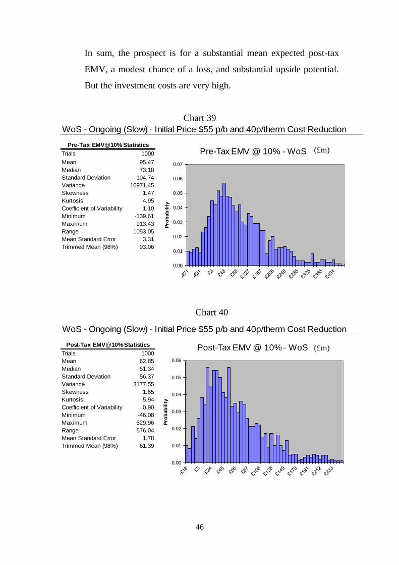
iv. W of S
The distribution of EMVs in the W of S region is shown in Chart
39 (pre-tax) and Chart 40 (post-tax). The mean value is healthily
positive at £95.47 million before tax, and £62.85 million after tax.
There is a chance of just over 14% that the pre-tax EMV will be
negative, and a 10% chance that it will be ‒£11.24 million or
worse. On the upside potential there is a 30% chance that the
EMV will exceed £131.08 million, and a 20% chance that it will
exceed +£164.4 million. 68% of the pre-tax EMV distribution lies
in the range +£4.91m. to +£187.54m., and 95% of the distribution
lies in the range -£54.8m. to +£361.85m. After tax the chance of
the EMV being negative is just over 6%, and there is a 20% chance
that it will exceed +£100.64 million. 68% of the post-tax EMV
distribution lies in the range +£14.81m. to +£112.71m., and 95% of
the distribution lies in the range -£10.24m. to +£206.91m.
SNS - Ongoing (Slow) - Initial Price $55 p/b and 40p/therm Cost Reduction
Post-Tax EMV@10% Statistics
Trials 1000
Mean 2.17
Median 1.75
Standard Deviation 2.01
Variance 4.03
Skewness 1.54
Kurtosis 4.08
Coefficient of Variability 0.92
Minimum -1.27
Maximum 14.78
Range 16.05
Mean Standard Error 0.06
Trimmed Mean (98%) 2.11
0.00
0.01
0.02
0.03
0.04
0.05
0.06
Pro
bab
ilit
y
Post-Tax EMV @ 10% - SNS (£m)
46
In sum, the prospect is for a substantial mean expected post-tax
EMV, a modest chance of a loss, and substantial upside potential.
But the investment costs are very high.
Chart 39
Chart 40
WoS - Ongoing (Slow) - Initial Price $55 p/b and 40p/therm Cost Reduction
Pre-Tax EMV@10% Statistics
Trials 1000
Mean 95.47
Median 73.18
Standard Deviation 104.74
Variance 10971.45
Skewness 1.47
Kurtosis 4.95
Coefficient of Variability 1.10
Minimum -139.61
Maximum 913.43
Range 1053.05
Mean Standard Error 3.31
Trimmed Mean (98%) 93.06
0.00
0.01
0.02
0.03
0.04
0.05
0.06
0.07P
rob
ab
ilit
y
Pre-Tax EMV @ 10% - WoS
WoS - Ongoing (Slow) - Initial Price $55 p/b and 40p/therm Cost Reduction
Post-Tax EMV@10% Statistics
Trials 1000
Mean 62.85
Median 51.34
Standard Deviation 56.37
Variance 3177.55
Skewness 1.65
Kurtosis 5.94
Coefficient of Variability 0.90
Minimum -46.08
Maximum 529.96
Range 576.04
Mean Standard Error 1.78
Trimmed Mean (98%) 61.39
0.00
0.01
0.02
0.03
0.04
0.05
0.06
Pro
bab
ilit
y
Post-Tax EMV @ 10% - WoS
(£m)
(£m)

47
(b) Project Investor, Slow Cycle Time.
i. CNS
The distribution of EMVs for the project investor in the CNS with
IA applicable to all exploration costs is shown in Chart 41 (post-
tax). There is a 68% chance that the EMV will be negative, and a
30% chance that it will exceed +£0.72 million. 68% of the post-tax
EMV distribution lies in the range -£20.81m. to +£6.53m., and
95% of the distribution lies in the range -£41.55m. to +£23.71m.
With a deterministic system where all variables are as the mean
values, the project investor with an oil find can write off his costs
and take advantage of the RFES, but he can only use 5% of the IA
to which he is entitled. The project investor with a gas find can
write off his costs, but can only take advantage of 23% of the
RFES, and he cannot use any of the IA to which he is entitled.
The prospect facing the investor is thus a combination of negative
mean expected post-tax EMV, a substantial downside risk, and
modest upside potential.

48
Chart 41
ii. NNS
The distribution of EMVs for the investor in the NNS with IA
allowance applicable to all exploration costs is shown in Chart 42
(post-tax). The mean value is negative to a modest extent. After
tax the chance of a negative EMV is 55%. 68% of the post-tax
EMV distribution lies in the range -£9.05m. to +£7.47m., and 95%
of the distribution lies in the range -£14.61m. to +£18.52m.
With a deterministic system where all variables are as the mean
values, the project investor with an oil find can write off his costs,
and take advantage of the RFES, but he can only use 5% of the IA
to which he is entitled. The project investor with a gas find can
write off his costs, but can only take advantage of 33% of the
RFES, and he cannot use any of the IA to which he is entitled.
CNS - Project (Slow) - Initial Price $55 p/b and 40p/therm Cost Reduction
Post-Tax EMV@10% Statistics
Trials 1000
Mean -7.15
Median -6.62
Standard Deviation 16.09
Variance 258.93
Skewness -0.26
Kurtosis 2.37
Coefficient of Variability -2.25
Minimum -85.08
Maximum 74.01
Range 159.10
Mean Standard Error 0.51
Trimmed Mean (98%) -7.07
0.00
0.01
0.02
0.03
0.04
0.05
0.06
0.07
Pro
bab
ilit
y
Post-Tax EMV @ 10% - CNS (£m)

49
The investor is thus faced with a combination of a (small) negative
mean expected EMV, a significant downside risk, and modest
upside potential.
Chart 42
iii. SNS
The distribution of EMVs for the investor in the SNS region is
shown in Chart 43 (post-tax). The chance of a negative EMV is
around 21% after tax. 68% of the post-tax EMV distribution lies in
the range -£0.42m. to +£4.21m., and 95% of the distribution lies in
the range -£1.88m. to +£7.71m.
With a deterministic system where all variables are as the mean
values, the project investor can write off his costs, take advantage
of the RFES, but can only use 36% of the IA to which he is
entitled.
In sum, the investor is faced with a very small positive mean EMV,
noteworthy downside risks, and very modest upside potential.
NNS - Project (Slow) - Initial Price $55 p/b and 40p/therm Cost Reduction
Post-Tax EMV@10% Statistics
Trials 1000
Mean -0.58
Median -1.23
Standard Deviation 8.71
Variance 75.82
Skewness 0.79
Kurtosis 2.04
Coefficient of Variability -14.90
Minimum -22.67
Maximum 55.20
Range 77.87
Mean Standard Error 0.28
Trimmed Mean (98%) -0.72
0.00
0.01
0.02
0.03
0.04
0.05
0.06
Pro
bab
ilit
y
Post-Tax EMV @ 10% - NNS (£m)

50
Chart 43
iv. W of S
The distribution of EMVs for the investor in the W of S region
with IA applicable to all exploration costs is shown in Chart 44
(post-tax). The mean value is healthily positive, at +£55.58 million
after tax. The chance of a negative EMV is 14%, and there is a
40% chance that the EMV will exceed +£61.63 million. There is a
20% chance that it will exceed +£98.62 million. 68% of the post-
tax EMV distribution lies in the range +£2.72m. to +£110.41m. and
95% of the distribution lies in the range -£52.53m. to +£204.68m.
With a deterministic system where all variables are as the mean
values, the project investor with an oil find can write off his costs,
take advantage of the RFES, and use 100% of the IA to which he is
entitled. The project investor with a gas find can write off his costs
and take advantage of the RFES, but he can only use 50% of the IA
to which he is entitled.
SNS - Project (Slow) - Initial Price $55 p/b and 40p/therm Cost Reduction
Post-Tax EMV@10% Statistics
Trials 1000
Mean 1.99
Median 1.79
Standard Deviation 2.44
Variance 5.94
Skewness 0.81
Kurtosis 1.58
Coefficient of Variability 1.23
Minimum -3.46
Maximum 14.90
Range 18.37
Mean Standard Error 0.08
Trimmed Mean (98%) 1.94
0.00
0.01
0.02
0.03
0.04
0.05
0.06
Pro
bab
ilit
y
Post-Tax EMV @ 10% - SNS (£m)

51
In sum, the investor is faced with a significantly positive mean
expected EMV, a modest risk of a loss (which in absolute terms
could be notable), and a substantial upside potential. But the
investment costs are very high in this region.
Chart 44
G. Tax Credit for Exploration Costs
(a) Project Investor, Slow Cycle Time.
i. CNS
The distribution of EMVs at 10% to the project investor in the
CNS with a tax credit under the slow cycle time assumptions with
reduced costs is shown in Chart 45 (post-tax). The mean value is
clearly negative. There is a greater than 67% chance that the EMV
will be negative. 68% of the post-tax EMV distribution lies in the
range -£18.81m. to +£6.55m., and 95% of the distribution lies in
the range -£39.56m. to +£22.89m.
With a deterministic system where all variables are as the mean
values, the project investor with an oil find and a tax credit can
WoS - Project (Slow) - Initial Price $55 p/b and 40p/therm Cost ReductionPost-Tax EMV@10% Statistics
Trials 1000
Mean 55.58
Median 47.09
Standard Deviation 62.30
Variance 3881.15
Skewness 1.00
Kurtosis 3.68
Coefficient of Variability 1.12
Minimum -136.24
Maximum 509.55
Range 645.80
Mean Standard Error 1.97
Trimmed Mean (98%) 54.71
0.00
0.01
0.02
0.03
0.04
0.05
0.06
Pro
bab
ilit
yPost-Tax EMV @ 10% - WoS (£m)

52
write off his costs and take advantage of the RFES (which is
reduced with the credit), but he can only use 26% of the IA to
which he is entitled. The project investor with a gas find and a tax
credit can write off his costs, but can only take advantage of 33%
of the (reduced) RFES, and he cannot use any of the IA to which
he is entitled.
In sum, the investor is faced with a negative mean expected EMV,
a very large downside risk, and a modest upside potential.
Chart 45
ii. NNS
The distribution of EMVs at 10% for the project investor in the
NNS with a tax credit and reduced costs is shown in Chart 46
(post-tax). The chance that the EMV will be negative is just over
47% after tax. 68% of the post-tax EMV distribution lies in the
range -£6.58m. to +£7.36m., and 95% of the distribution lies in the
range -£12.14m. to +£17.34m.
CNS - Project (Slow) Tax Credit - Initial Price $55 p/b and 40p/therm Reduced Costs
Post-Tax EMV@10% Statistics
Trials 1000
Mean -5.95
Median -4.86
Standard Deviation 15.34
Variance 235.17
Skewness -0.36
Kurtosis 2.83
Coefficient of Variability -2.58
Minimum -83.09
Maximum 73.63
Range 156.71
Mean Standard Error 0.48
Trimmed Mean (98%) -5.86
0.00
0.01
0.02
0.03
0.04
0.05
0.06
0.07
Pro
bab
ilit
y
Post-Tax EMV @ 10% - CNS (£m)

53
With a deterministic system where all variables are as the mean
values, the project investor with an oil find and a tax credit can
write off his costs and take advantage of the RFES (which is
reduced with the credit), but can only use 66% of the IA to which
he is entitled. The project investor with a gas find and a tax credit
can write off his costs, and take advantage of the (reduced) RFES,
but he can only use 61% of the IA to which he is entitled.
In sum, the investor is faced with a tiny positive mean EMV, a very
large downside risk, and a modest upside potential.
Chart 46
iii. SNS
The distribution of EMVs for the project investor in the SNS with a
tax credit and reduced costs is shown in Chart 47 (post-tax).
There is a 13% chance that the post-tax EMV will be negative.
68% of the post-tax distribution lies in the range +£0.16m. to
+£3.97m., and 95% lies in the range -£1.13m. to +£7.25m.
NNS - Project (Slow) Tax Credit - Initial Price $55 p/b and 40p/therm Reduced Costs
Post-Tax EMV@10% Statistics
Trials 1000
Mean 0.67
Median 0.38
Standard Deviation 7.59
Variance 57.54
Skewness 0.88
Kurtosis 3.28
Coefficient of Variability 11.38
Minimum -20.20
Maximum 54.27
Range 74.47
Mean Standard Error 0.24
Trimmed Mean (98%) 0.55
0.00
0.01
0.02
0.03
0.04
0.05
0.06
Pro
bab
ilit
y
Post-Tax EMV @ 10% - NNS (£m)

54
With a deterministic system where all variables are as the mean
values, the project investor with a tax credit for exploration can
write off his costs, take advantage of the (reduced) RFES, but can
only use 95% of the IA to which he is entitled.
Chart 47
iv. W of S
The distribution of EMVs for the project investor in the W of S
region with a tax credit and reduced costs is shown in Chart 48
(post-tax). The chance of the EMV being negative is 13%. There
is a 20% chance that the value will be +£96.62 million or better.
68% of the post-tax EMV distribution lies in the range +£3.75m. to
+£108.63m., and 95% of the distribution lies in the range -
£48.25m. to +£202.87m.
With a deterministic system where all variables are as the mean
values, the project investor with an oil find and a tax credit for
exploration can write off his costs, take advantage of the RFES,
SNS - Project (Slow) Tax Credit - Initial Price $55 p/b and 40p/therm Reduced Costs
Post-Tax EMV@10% Statistics
Trials 1000
Mean 2.09
Median 1.80
Standard Deviation 2.12
Variance 4.50
Skewness 1.13
Kurtosis 2.80
Coefficient of Variability 1.01
Minimum -2.72
Maximum 14.58
Range 17.30
Mean Standard Error 0.07
Trimmed Mean (98%) 2.05
0.00
0.01
0.02
0.03
0.04
0.05
0.06
Pro
bab
ilit
yPost-Tax EMV @ 10% - SNS (£m)

55
and use 100% of the IA to which he is entitled. The project
investor with a gas find and a tax credit can write off his costs and
take advantage of the (reduced) RFES, but he can only use 67% of
the IA to which he is entitled.
In sum, the investor is faced with a worthwhile mean expected
EMV, modest downside risk and substantial upside potential. But
the investment costs are very high.
Chart 48
H. Investment Allowance Restricted to Successful Exploration
(a) Investor in Tax-Paying Position, Slow Cycle Time
i. CNS
When the cycle time from first exploration to first production
becomes longer and extra appraisal costs are incurred the
discounted expected returns are reduced. When the IA for
exploration is limited and costs are reduced there is a more than
48% chance that the post-tax EMV will be negative. 68% of the
WoS - Project (Slow) Tax Credit - Initial Price $55 p/b and 40p/therm Reduced Costs
Post-Tax EMV@10% Statistics
Trials 1000
Mean 55.19
Median 45.35
Standard Deviation 60.86
Variance 3704.53
Skewness 1.09
Kurtosis 4.04
Coefficient of Variability 1.10
Minimum -131.96
Maximum 508.38
Range 640.34
Mean Standard Error 1.92
Trimmed Mean (98%) 54.29
0.00
0.01
0.02
0.03
0.04
0.05
0.06
0.07
Pro
bab
ilit
y
Post-Tax EMV @ 10% - WoS (£m)

56
post-tax EMV distribution lies in the range -£6.78m. to +£9.08m.,
and 95% of the distribution lies in the range -£16.83m. to +£25.5m.
In sum, the investor is faced with the prospect of a positive but tiny
mean expected EMV, a high chance of a loss, and modest upside
potential.
Chart 49
ii. NNS
When the key risks are considered and the IA for exploration is
limited and costs are reduced the distribution of EMVs at 10% are
shown in Chart 50 (post-tax). The chance of a negative EMV is
39% after tax. 68% of the post-tax EMV distribution lies in the
range -£2.79m. to +£7.43m. and 95% of the distribution lies in the
range -£5.09m. to +£17.36m.
In sum, the investor is faced with a very small positive expected
mean EMV, a substantial risk of a loss, and very modest upside
potential.
CNS - Ongoing (Slow) Limited IA - Initial Price $55 p/b and 40p/therm Reduced Costs
Post-Tax EMV@10% Statistics
Trials 1000
Mean 1.24
Median 0.17
Standard Deviation 10.22
Variance 104.47
Skewness 1.18
Kurtosis 5.89
Coefficient of Variability 8.24
Minimum -34.05
Maximum 81.10
Range 115.16
Mean Standard Error 0.32
Trimmed Mean (98%) 1.08
0.00
0.01
0.02
0.03
0.04
0.05
0.06
0.07
0.08
Pro
bab
ilit
y
Post-Tax EMV @ 10% - CNS (£m)
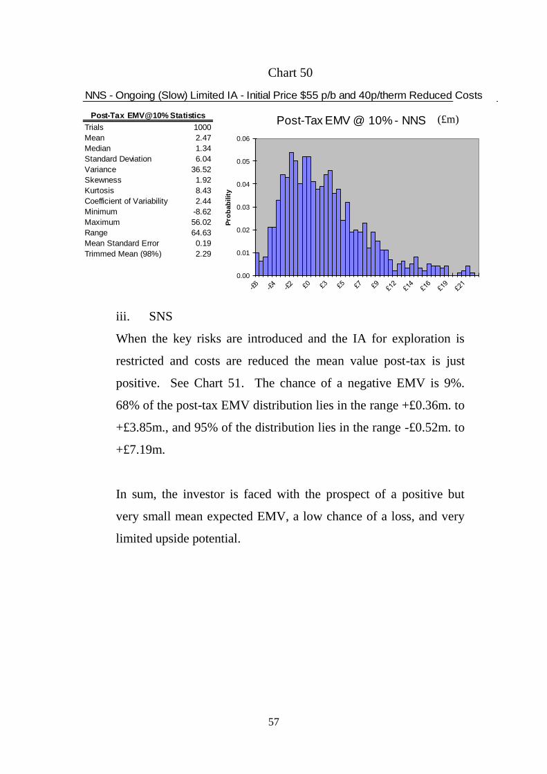
57
Chart 50
iii. SNS
When the key risks are introduced and the IA for exploration is
restricted and costs are reduced the mean value post-tax is just
positive. See Chart 51. The chance of a negative EMV is 9%.
68% of the post-tax EMV distribution lies in the range +£0.36m. to
+£3.85m., and 95% of the distribution lies in the range -£0.52m. to
+£7.19m.
In sum, the investor is faced with the prospect of a positive but
very small mean expected EMV, a low chance of a loss, and very
limited upside potential.
NNS - Ongoing (Slow) Limited IA - Initial Price $55 p/b and 40p/therm Reduced Costs
Post-Tax EMV@10% Statistics
Trials 1000
Mean 2.47
Median 1.34
Standard Deviation 6.04
Variance 36.52
Skewness 1.92
Kurtosis 8.43
Coefficient of Variability 2.44
Minimum -8.62
Maximum 56.02
Range 64.63
Mean Standard Error 0.19
Trimmed Mean (98%) 2.29
0.00
0.01
0.02
0.03
0.04
0.05
0.06
Pro
bab
ilit
y
Post-Tax EMV @ 10% - NNS (£m)

58
Chart 51
iv. W of S
When the key risks are considered and the IA for exploration is
limited and costs are reduced the distribution of EMVs at 10% is
shown in Chart 52 (post-tax). The mean values are positive before
tax and after tax. After tax there is more than a 6% chance that the
EMV will be negative. There is a 20% chance that the EMV will
exceed +£100.52 million, and a 10% chance that it exceeds
+£136.18 million. 68% of the post-tax EMV distribution lies in the
range +£14.69m. to +£112.54m., and 95% of the distribution lies in
the range -£10.32m. to +£206.75m.
In sum, the investor is faced with the prospect of a significantly
positive mean expected EMV, a small chance of a loss, and very
substantial upside potential. The investment costs are particularly
large in this region.
SNS - Ongoing (Slow) Limited IA - Initial Price $55 p/b and 40p/therm Reduced Costs
Post-Tax EMV@10% Statistics
Trials 1000
Mean 2.13
Median 1.71
Standard Deviation 2.01
Variance 4.03
Skewness 1.54
Kurtosis 4.08
Coefficient of Variability 0.94
Minimum -1.30
Maximum 14.74
Range 16.04
Mean Standard Error 0.06
Trimmed Mean (98%) 2.08
0.00
0.01
0.02
0.03
0.04
0.05
0.06
Pro
bab
ilit
y
Post-Tax EMV @ 10% - SNS (£m)

59
Chart 52
(b) Project Investor, Slow Cycle Time
i. CNS
The distribution of EMVs at 10% to the project investor in the
CNS under the slow cycle time assumptions with restricted IA for
exploration and reduced costs is shown in Chart 53 (post-tax).
There is a greater than 68% chance that the EMV will be negative.
68% of the post-tax distribution lies in the range -£20.81m. to
+£6.53m., and 95% of the distribution lies in the range -£41.55m.
to +£23.63m.
With a deterministic system where all variables are as the mean
values, with limited IA the project investor with an oil find can
write off his costs and take advantage of the RFES, but he can only
use 6% of the IA to which he is entitled. The project investor with
a gas find can write off his costs, but can only take advantage of
23% of the RFES, and he cannot use any of the IA to which he is
entitled.
WoS - Ongoing (Slow) Limited IA - Initial Price $55 p/b and 40p/therm Reduced Costs
Post-Tax EMV@10% Statistics
Trials 1000
Mean 62.71
Median 51.18
Standard Deviation 56.36
Variance 3175.89
Skewness 1.65
Kurtosis 5.95
Coefficient of Variability 0.90
Minimum -46.14
Maximum 529.82
Range 575.96
Mean Standard Error 1.78
Trimmed Mean (98%) 61.25
0.00
0.01
0.02
0.03
0.04
0.05
0.06
Pro
bab
ilit
y
Post-Tax EMV @ 10% - WoS (£m)

60
In sum, the investor is faced with the prospect of a negative mean
expected EMV, a very high chance of a loss, and limited upside
potential.
Chart 53
ii. NNS
The distribution of EMVs at 10% for the project investor in the
NNS with limited IA for exploration and reduced costs is shown in
Chart 54 (post-tax). The chance that the EMV will be negative is
over 55%. 68% of the post-tax EMV distribution lies in the range -
£9.05m. to +£7.47m., and 95% of the distribution lies in the range -
£14.61m. to +£18.44m.
With a deterministic system where all variables are as the mean
values with limited IA the project investor with an oil find can
write off his costs and take advantage of the RFES, but he can only
use 6% of the IA to which he is entitled. The project investor with
a gas find can write off his costs, but can only take advantage of
CNS - Project (Slow) Limited IA - Initial Price $55 p/b and 40p/therm Reduced Costs
Post-Tax EMV@10% Statistics
Trials 1000
Mean -7.16
Median -6.62
Standard Deviation 16.08
Variance 258.67
Skewness -0.26
Kurtosis 2.37
Coefficient of Variability -2.25
Minimum -85.08
Maximum 73.97
Range 159.05
Mean Standard Error 0.51
Trimmed Mean (98%) -7.08
0.00
0.01
0.02
0.03
0.04
0.05
0.06
0.07P
rob
ab
ilit
y
Post-Tax EMV @ 10% - CNS (£m)

61
33% of the RFES, and he cannot use any of the IA to which he is
entitled
In sum, the investor is faced with the prospect of a small negative
mean expected EMV, a large chance of a loss, and very limited
upside potential
Chart 54
iii. SNS
The distribution of EMVs for the project investor in the SNS with
limited IA for exploration and reduced costs is shown in Chart 55
(post-tax). There is a more than 21% chance that the value will be
negative. 68% of the post-tax distribution lies in the range -
£0.42m. to +£4.21m., and 95% lies in the range -£1.88m. to
+£7.68m.
With a deterministic system where all variables are as the mean
values, with limited IA the project investor can write off his costs,
take advantage of the (reduced) RFES, but can only use 38% of the
IA to which he is entitled.
NNS - Project (Slow) Limited IA - Initial Price $55 p/b and 40p/therm Reduced Costs
Post-Tax EMV@10% Statistics
Trials 1000
Mean -0.59
Median -1.23
Standard Deviation 8.69
Variance 75.60
Skewness 0.78
Kurtosis 2.03
Coefficient of Variability -14.72
Minimum -22.67
Maximum 55.11
Range 77.78
Mean Standard Error 0.27
Trimmed Mean (98%) -0.72
0.00
0.01
0.02
0.03
0.04
0.05
0.06
Pro
bab
ilit
y
Post-Tax EMV @ 10% - NNS (£m)

62
In sum, the investor is faced with the prospect of a positive but
very small mean expected EMV, a moderate chance of a loss, and
very limited upside potential.
Chart 55
iv. W of S
The distribution of EMVs for the project investor in the W of S
region with IA limited for exploration and reduced costs is shown
in Chart 56 (post-tax). The chance of the EMV being negative is
14%. There is a 20% chance that the value will be +£98.47 million
or better. 68% of the post-tax EMV distribution lies in the range
+£2.72m. to +£110.27m., and 95% of the distribution lies in the
range -£52.53m. to +£204.53m.
With a deterministic system where all variables are as the mean
values, with limited IA the project investor with an oil find can
write off his costs and take advantage of the RFES, and he can use
SNS - Project (Slow) Limited IA - Initial Price $55 p/b and 40p/therm Reduced Costs
Post-Tax EMV@10% Statistics
Trials 1000
Mean 1.98
Median 1.79
Standard Deviation 2.43
Variance 5.90
Skewness 0.80
Kurtosis 1.58
Coefficient of Variability 1.23
Minimum -3.46
Maximum 14.87
Range 18.34
Mean Standard Error 0.08
Trimmed Mean (98%) 1.94
0.00
0.01
0.02
0.03
0.04
0.05
0.06
Pro
bab
ilit
yPost-Tax EMV @ 10% - SNS (£m)
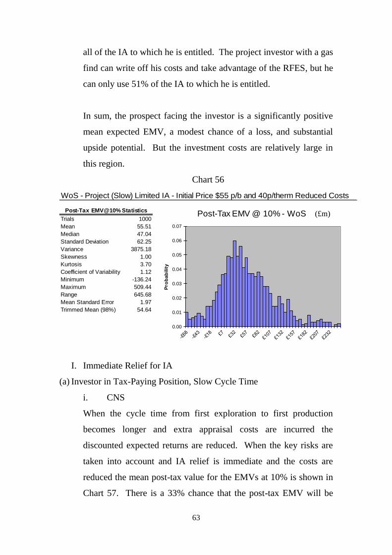
63
all of the IA to which he is entitled. The project investor with a gas
find can write off his costs and take advantage of the RFES, but he
can only use 51% of the IA to which he is entitled.
In sum, the prospect facing the investor is a significantly positive
mean expected EMV, a modest chance of a loss, and substantial
upside potential. But the investment costs are relatively large in
this region.
Chart 56
I. Immediate Relief for IA
(a) Investor in Tax-Paying Position, Slow Cycle Time
i. CNS
When the cycle time from first exploration to first production
becomes longer and extra appraisal costs are incurred the
discounted expected returns are reduced. When the key risks are
taken into account and IA relief is immediate and the costs are
reduced the mean post-tax value for the EMVs at 10% is shown in
Chart 57. There is a 33% chance that the post-tax EMV will be
WoS - Project (Slow) Limited IA - Initial Price $55 p/b and 40p/therm Reduced Costs
Post-Tax EMV@10% Statistics
Trials 1000
Mean 55.51
Median 47.04
Standard Deviation 62.25
Variance 3875.18
Skewness 1.00
Kurtosis 3.70
Coefficient of Variability 1.12
Minimum -136.24
Maximum 509.44
Range 645.68
Mean Standard Error 1.97
Trimmed Mean (98%) 54.64
0.00
0.01
0.02
0.03
0.04
0.05
0.06
0.07
Pro
bab
ilit
y
Post-Tax EMV @ 10% - WoS (£m)

64
negative. 68% of the post-tax EMV distribution lies in the range -
£3.41m. to +£12.02m., and 95% of the distribution lies in the range
-£9.46m. to +£27.53m.
In sum, the prospect facing the investor is a positive but small
mean expected EMV, a substantial risk of a loss, and moderate
upside potential.
Chart 57
ii. NNS
When the key risks are considered and IA relief is immediate and
costs are reduced the distribution of EMVs at 10% are shown in
Chart 58 (post-tax). The chance of a negative EMV is 24%. 68%
of the post-tax EMV distribution lies in the range -£1.09m. to
+£9.12m., and 95% of the distribution lies in the range -£3.42m. to
+£19.17m.
CNS - Ongoing (Slow Tax Saved) - Initial Price $55 p/b and 40p/therm Cost Reduction
Post-Tax EMV@10% Statistics
Trials 1000
Mean 4.48
Median 2.94
Standard Deviation 9.66
Variance 93.24
Skewness 1.85
Kurtosis 9.00
Coefficient of Variability 2.15
Minimum -20.12
Maximum 90.98
Range 111.10
Mean Standard Error 0.31
Trimmed Mean (98%) 4.23
0.00
0.01
0.02
0.03
0.04
0.05
0.06
0.07
Pro
bab
ilit
y
Post-Tax EMV @ 10% - CNS (£m)

65
In sum, the prospect facing the investor is a positive but small
mean expected EMV, a significant risk of a loss, and very modest
upside potential.
Chart 58
iii. SNS
When the key risks are introduced, relief for IA is immediate, and
costs are reduced the mean expected value post-tax is shown in
Chart 59. After tax the chance of a negative EMV is only 3%.
68% of the post-tax EMV distribution lies in the range +£0.86m. to
+£4.45m., and 95% of the distribution lies in the range -£0.06m. to
+£7.69m.
In sum, the prospect facing the investor is a positive but very small
mean expected EMV, a small downside risk, and a very small
upside potential.
NNS - Ongoing (Slow Tax Saved) - Initial Price $55 p/b and 40p/therm Cost Reduction
Post-Tax EMV@10% Statistics
Trials 1000
Mean 4.22
Median 3.05
Standard Deviation 6.11
Variance 37.37
Skewness 2.01
Kurtosis 9.28
Coefficient of Variability 1.45
Minimum -5.69
Maximum 60.13
Range 65.82
Mean Standard Error 0.19
Trimmed Mean (98%) 4.03
0.00
0.01
0.02
0.03
0.04
0.05
0.06
Pro
bab
ilit
y
Post-Tax EMV @ 10% - NNS (£m)

66
Chart 59
iv. W of S
When the key risks are considered, relief for IA is immediate, and
costs are reduced the distribution of EMVs at 10% is shown in
Chart 60 (post-tax). There is only a 1% chance that the EMV will
be negative. There is a 20% chance that the EMV will exceed
+£108.23 million, and a 10% chance that it exceeds +£142.59
million. 68% of the post-tax EMV distribution lies in the range
+£21.51m. to +£119.32m., and 95% of the distribution lies in the
range +£2.78m. to +£216.31m.
In sum, the prospect facing the investor is a substantial mean
expected EMV, low risk of a loss, and substantial potential. But
the investment costs are notably high.
SNS - Ongoing (Slow Tax Saved) - Initial Price $55 p/b and 40p/therm Cost Reduction
Post-Tax EMV@10% Statistics
Trials 1000
Mean 2.67
Median 2.26
Standard Deviation 2.07
Variance 4.30
Skewness 1.51
Kurtosis 3.93
Coefficient of Variability 0.78
Minimum -0.83
Maximum 15.59
Range 16.41
Mean Standard Error 0.07
Trimmed Mean (98%) 2.61
0.00
0.01
0.02
0.03
0.04
0.05
0.06
Pro
bab
ilit
y
Post-Tax EMV @ 10% - SNS (£m)

67
Chart 60
J. Interest on Unutilised IA from time of Eligibility of Activation
(a) Project Investor, Slow Cycle Time
i. CNS
The distribution of EMVs at 10% to the project investor in the
CNS under the slow cycle time assumptions with interest on IA
and reduced costs is shown in Chart 61 (post-tax). There is a
greater than 67% chance that the EMV will be negative. 68% of
the post-tax EMV distribution lies in the range -£20.81m. to
+£9.81m., and 95% of the distribution lies in the range -£41.55m.
to +£39.23m.
With a deterministic system where all variables are as the mean
values and interest is given on unused IA, the project investor with
an oil find can write off his costs but can only use 3% of his RFES,
and cannot use any of the IA to which he is entitled. With a gas
find and interest on unused IA the project investor can write off his
WoS - Ongoing (Slow Tax Saved) - Initial Price $55 p/b and 40p/therm Cost Reduction
Post-Tax EMV@10% Statistics
Trials 1000
Mean 70.21
Median 57.31
Standard Deviation 56.09
Variance 3146.04
Skewness 1.83
Kurtosis 7.25
Coefficient of Variability 0.80
Minimum -17.10
Maximum 562.85
Range 579.95
Mean Standard Error 1.77
Trimmed Mean (98%) 68.56
0.00
0.01
0.02
0.03
0.04
0.05
0.06
Pro
bab
ilit
y
Post-Tax EMV @ 10% - WoS (£m)

68
costs but he can only use 1% of his RFES, and none of the IA to
which he is entitled.
In sum, the prospect facing the investor is a negative mean
expected EMV, a large risk of a loss, and modest upside potential.
Chart 61
ii. NNS
The distribution of EMVs at 10% for the project investor in the
NNS with interest on IA and reduced costs is shown in Chart 62
(post-tax). The chance that the EMV will be negative is over 55%.
68% of the post-tax EMV distribution lies in the range -£9.05m. to
+£9.75m., and 95% of the distribution lies in the range -£14.61m.
to +£28.4m.
With a deterministic system where all variables are as the mean
values and interest is given on unused IA, the project investor with
an oil find can write off his costs but can only use 4% of his RFES,
CNS - Project (Slow Interest on IA) - Initial Price $55 p/b and 40p/therm Cost Reduction
Post-Tax EMV@10% Statistics
Trials 1000
Mean -5.39
Median -6.59
Standard Deviation 19.28
Variance 371.59
Skewness 0.68
Kurtosis 3.94
Coefficient of Variability -3.58
Minimum -85.08
Maximum 120.56
Range 205.64
Mean Standard Error 0.61
Trimmed Mean (98%) -5.55
0.00
0.01
0.02
0.03
0.04
0.05
0.06
0.07
Pro
bab
ilit
y
Post-Tax EMV @ 10% - CNS (£m)

69
and cannot use any of the IA to which he is entitled. With a gas
find and interest on unused IA the project investor can write off his
costs, but he can only use 2% of his RFES, and none of the IA to
which he is entitled.
In sum, the prospect facing the investor is a positive but tiny mean
expected EMV, a substantial risk of a loss, and modest upside
potential.
Chart 62
iii. SNS
The distribution of EMVs for the project investor in the SNS with
interest on IA and reduced costs is shown in Chart 63 (post-tax).
There is a 21% chance that the post-tax EMV will be negative.
68% of the post-tax distribution lies in the range -£0.42m. to
+£5.95m., and 95% lies in the range -£1.88m. to +£12.36m.
With a deterministic system where all variables are as the mean
values and interest is given on unused IA the project investor can
NNS - Project (Slow Interest on IA) - Initial Price $55 p/b and 40p/therm Cost Reduction
Post-Tax EMV@10% Statistics
Trials 1000
Mean 0.62
Median -1.21
Standard Deviation 11.18
Variance 124.96
Skewness 1.75
Kurtosis 7.04
Coefficient of Variability 18.15
Minimum -22.67
Maximum 94.08
Range 116.75
Mean Standard Error 0.35
Trimmed Mean (98%) 0.31
0.00
0.01
0.02
0.03
0.04
0.05
0.06
0.07
Pro
bab
ilit
y
Post-Tax EMV @ 10% - NNS (£m)

70
write off his costs, but he can only use 5% of his RFES, and none
of the IA to which he is entitled.
In sum, the prospect facing the investor is a positive but small
mean expected EMV, significant risk of a loss, and modest upside
potential.
Chart 63
iv. W of S
The distribution of EMVs for the project investor in the W of S
region with interest on IA and reduced costs is shown in Chart 64
(post-tax). The chance of the EMV being negative is 13%, with a
20% chance that it will be +£16.06 million or worse. There is a
20% chance that the value will be +£164.53 million or better.
68% of the post-tax EMV distribution lies in the range +£6.55m. to
+£179.95m., and a 95% of the distribution lies in the range -
£52.53m. to +£325.9m.
SNS - Project (Slow Interest on IA) - Initial Price $55 p/b and 40p/therm Cost Reduction
Post-Tax EMV@10% Statistics
Trials 1000
Mean 2.78
Median 1.96
Standard Deviation 3.63
Variance 13.17
Skewness 1.55
Kurtosis 3.97
Coefficient of Variability 1.31
Minimum -3.46
Maximum 25.33
Range 28.80
Mean Standard Error 0.11
Trimmed Mean (98%) 2.67
0.00
0.01
0.02
0.03
0.04
0.05
0.06
0.07
Pro
bab
ilit
y
Post-Tax EMV @ 10% - SNS (£m)

71
With a deterministic system where all variables are as the mean
values and interest is given on unused IA, the project investor with
an oil find can write off his costs, but can only use 8% of his
RFES, and none of the IA to which he is entitled. With a gas find
and interest on unused IA the project investor can write off his
costs, but he can only use 5% of his RFES, and none of the IA to
which he is entitled.
In sum, the prospect facing the investor is a substantial mean
expected EMV, a modest risk of a loss, and a large upside
potential. But the investment costs are very large in this region.
Chart 64
K. Comparison of Results
Table 3 below allows a ready comparison of the various systems with a
fast cycle time. After the cost reductions employed in this study it is seen
that the mean expected EMVs are positive in 3 of the regions, the
exception being the CNS. In this latter area the investment costs per boe
WoS - Project (Slow Interest on IA) - Initial Price $55 p/b and 40p/therm Cost Reduction
Post-Tax EMV@10% Statistics
Trials 1000
Mean 93.37
Median 75.16
Standard Deviation 97.20
Variance 9447.83
Skewness 1.37
Kurtosis 5.75
Coefficient of Variability 1.04
Minimum -136.24
Maximum 919.75
Range 1056.00
Mean Standard Error 3.07
Trimmed Mean (98%) 91.39
0.00
0.01
0.02
0.03
0.04
0.05
0.06
Pro
bab
ilit
y
Post-Tax EMV @ 10% - WoS (£m)

72
are relatively high. The highest prospective returns are in the W of S
region. This reflects the relatively high success rate and the
comparatively large sizes of discoveries. This latter factor reduces the
investment costs per boe, though in absolute terms they are highest of all
the regions in the UKCS.
It is also seen from Table 3 that the mean post-tax EMVs are higher for
the investor already in a tax-paying position compared to the project
investor. The chances of making a loss are also greater for the project
investor compared to one already in a tax-paying position. A fully
neutral tax system should not discriminate in this way. This does not
only result in circumstances when the investor’s discount rate exceeds the
RFES interest rate. In the study many cases were found where the project
investor could not obtain the full benefits from the IA and the RFES to
which he was entitled because of lack of adequate income against which
to set the allowance. This happens for investors in the CNS, NNS, and W
of S to a greater extent than in the SNS where the probability of a
negative return is generally low. Thus both the mean expected EMV and
the range of EMVs in the SNS for the project investor are quite close to
those obtained by the tax-paying investor.
When further tax incentives were examined it was found that the project
investors were often less able to take advantage of them compared to the
investor already in a tax-paying position because of inadequate income.
This helps to explain the finding that of all the further tax incentives
considered in this study the most potent for the tax-paying investor differs
from that for the project investor. Thus, for the investor already in a tax-
paying position the most potent further incentive in all the four regions of
the UKCS is immediate tax relief for the IA. For the project investor the

73
most potent extra incentive was found to be interest on the IA eligible for
activation. Of course, the investor already in a tax-paying position should
not have a need for this facility.
Table 3
Comparative Returns After Cost Reductions, Fast Cycle Time
Tax-Paying Investor, Fast Cycle Time, full IA relief CNS NNS SNS W of S Pre-Tax Mean EMV (£m.) -2.40 6.68 5.13 126.46
68% of EMV range (£m.) -21.76 to +15.63 -4.78 to +17.68 +1.26 to +8.98 +16.09 to +237.27
95% of EMV range (£m.) -45.01 to +52.61 -11.58 to +41.6 -0.58 to +16.36 -54.63 to +452.22
Chance of negative EMV 58% 34% 5% 10%
30% Chance EMV will Exceed (£m.) 5.72 10.75 6.42 168.85
Post-Tax Mean EMV (£m.) 4.03 6.12 3.52 81.17
68% of EMV range (£m.) -5.79 to +13.55 -0.26 to +12.1 +1.39 to +5.56 +21.97 to +140.44
95% of EMV range (£m.) -16.99 to +34.62 -3.16 to +24.23 +0.29 to +9.57 -7.83 to +264.01
Chance of negative EMV 37% 19% 1% 4%
30% Chance EMV will Exceed (£m.) 8.00 8.22 4.24 101.38
Project Investor, Fast Cycle Time, full IA Relief
Post-Tax Mean EMV (£m.) -4.58 4.02 3.44 71.82
68% of EMV range (£m.) -20.59 to +10.17 -4.4 to +11.76 +1.12 to +5.64 +10.11 to +134.73
95% of EMV range (£m.) -43.24 to +30.79 -10.9 to +24.72 -0.51 to +9.72 -52.24 to +253.67
Chance of negative EMV 59% 33% 4% 11%
30% Chance EMV will Exceed (£m.) 3.86 7.64 4.36 97.02
Project Investor, Fast Cycle Time Tax Credit
Post-Tax Mean EMV (£m.) -3.51 4.67 3.38 71.92
68% of EMV range (£m.) -18.59 to +10.11 -2.17 to +11.25 +1.21 to +5.41 +11.15 to +134.27
95% of EMV range (£m.) -41.25 to +30.52 -8.43 to +23.87 -0.04 to +9.52 -47.96 to +249.25
Chance of negative EMV 56% 26% 3% 10%
30% Chance EMV will Exceed (£m.) 4.22 7.53 4.15 96.66
Tax-Paying Investor, Fast Cycle Time IA limited
Post-Tax Mean EMV (£m.) 3.95 5.98 3.47 80.99

74
68% of EMV range (£m.) -5.87 to +13.43 -0.4 to +11.94 +1.33 to +5.51 +21.81 to +140.25
95% of EMV range (£m.) -16.99 to +34.51 -3.27 to +24.07 +0.24 to +9.52 -7.95 to +263.8
Chance of negative EMV 38% 19% 1% 4%
30% Chance EMV will Exceed (£m.) 7.91 8.07 4.19 101.20
Project Investor, Fast Cycle Time IA limited
Post-Tax Mean EMV (£m.) -4.59 3.99 3.42 71.72
68% of EMV range (£m.) -20.59 to +10.10 -4.4 to +11.68 +1.12 to +5.6 +10.11 to +134.64
95% of EMV range (£m.) -43.24 to +30.69 -10.9 to +24.62 -0.51 to +9.68 -52.24 to +253.51
Chance of negative EMV 58% 33% 4% 11%
30% Chance EMV will Exceed (£m.) 3.86 7.64 4.32 96.88
Tax-Paying Investor, Fast Cycle Time immediate IA relief
Post-Tax Mean EMV (£m.) 7.36 7.53 3.96 89.03
68% of EMV range (£m.) -2.07 to +16.51 +1.05 to +13.58 +1.73 to +6.11 +29.65 to +148.2
95% of EMV range (£m.) -8.99 to +36.84 -1.77 to +25.78 +0.6 to +10.14 +8.45 to +268.59
Chance of negative EMV 24% 8% 1% 1%
30% Chance EMV will Exceed (£m.) 10.65 9.80 4.74 107.84
Project Investor, Fast Cycle Time interest on IA
Post-Tax Mean EMV (£m.) -1.40 7.13 5.28 120.76
68% of EMV range (£m.) -20.59 to +16.58 -4.4 to +18.19 +1.39 to +9.18 +17.98 to +219.9
95% of EMV range (£m.) -43.24 to +53.46 -10.9 to +41 -0.51 to +16.45 -52.24 to +385.18
Chance of negative EMV 56% 32% 4% 10%
30% Chance EMV will Exceed (£m.) 6.45 11.13 6.59 163.09
The mean expected pre-tax EMVs are seen to be positive in 3 of the 4
regions, but the values are clearly less than the case with the fast cycle
time, reflecting the larger appraisal costs and the longer time to first
production. The prospective return is highest in the W of S region. In the
other 3 regions the expected returns to a tax-paying investor are low.
Prospective returns to project investors are distinctly below these to the
tax-paying investor, with a notably greater chance of making a loss. Even
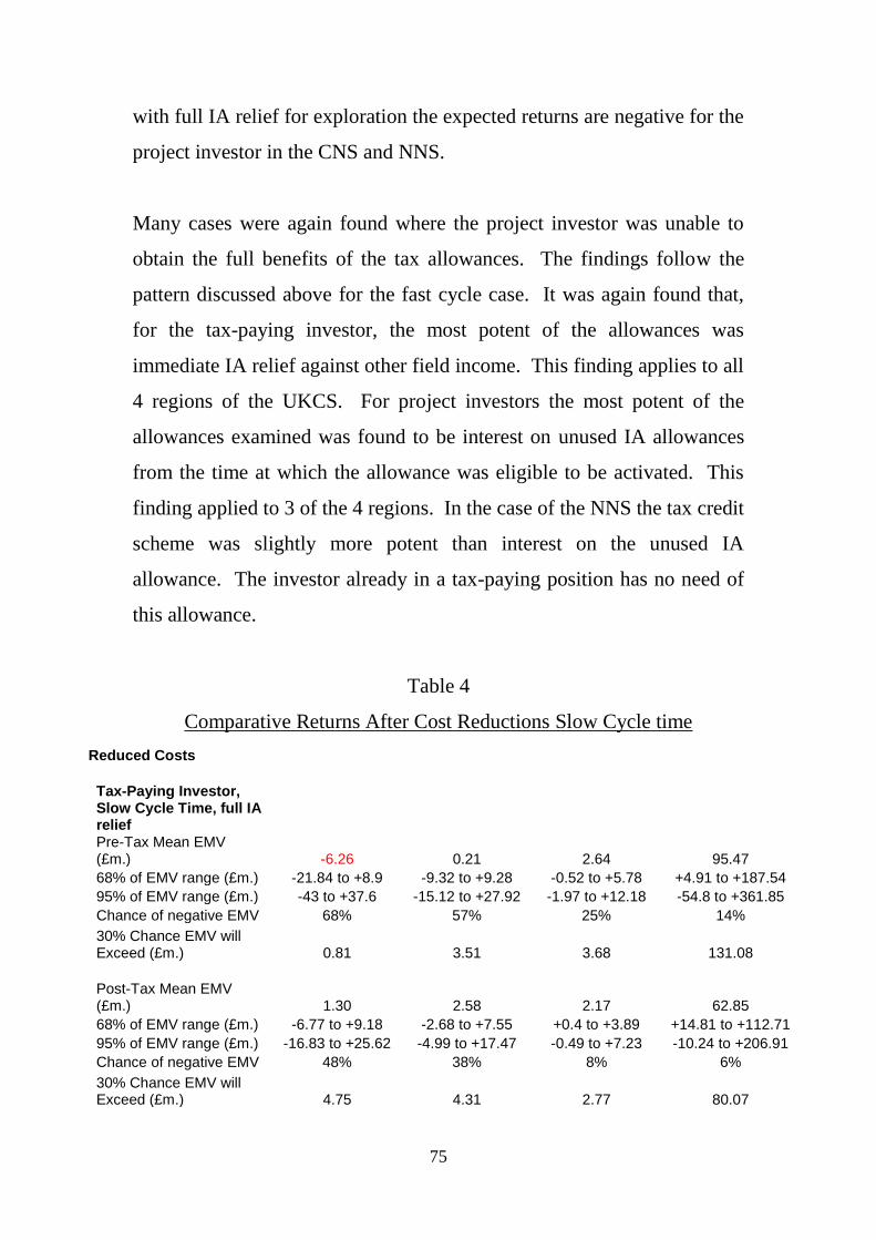
75
with full IA relief for exploration the expected returns are negative for the
project investor in the CNS and NNS.
Many cases were again found where the project investor was unable to
obtain the full benefits of the tax allowances. The findings follow the
pattern discussed above for the fast cycle case. It was again found that,
for the tax-paying investor, the most potent of the allowances was
immediate IA relief against other field income. This finding applies to all
4 regions of the UKCS. For project investors the most potent of the
allowances examined was found to be interest on unused IA allowances
from the time at which the allowance was eligible to be activated. This
finding applied to 3 of the 4 regions. In the case of the NNS the tax credit
scheme was slightly more potent than interest on the unused IA
allowance. The investor already in a tax-paying position has no need of
this allowance.
Table 4
Comparative Returns After Cost Reductions Slow Cycle time
Reduced Costs
Tax-Paying Investor, Slow Cycle Time, full IA relief
Pre-Tax Mean EMV (£m.) -6.26 0.21 2.64 95.47
68% of EMV range (£m.) -21.84 to +8.9 -9.32 to +9.28 -0.52 to +5.78 +4.91 to +187.54
95% of EMV range (£m.) -43 to +37.6 -15.12 to +27.92 -1.97 to +12.18 -54.8 to +361.85
Chance of negative EMV 68% 57% 25% 14%
30% Chance EMV will Exceed (£m.) 0.81 3.51 3.68 131.08
Post-Tax Mean EMV (£m.) 1.30 2.58 2.17 62.85
68% of EMV range (£m.) -6.77 to +9.18 -2.68 to +7.55 +0.4 to +3.89 +14.81 to +112.71
95% of EMV range (£m.) -16.83 to +25.62 -4.99 to +17.47 -0.49 to +7.23 -10.24 to +206.91
Chance of negative EMV 48% 38% 8% 6%
30% Chance EMV will Exceed (£m.) 4.75 4.31 2.77 80.07

76
Project Investor, Slow Cycle Time, full IA Relief
Post-Tax Mean EMV (£m.) -7.15 -0.58 1.99 55.58
68% of EMV range (£m.) -20.81 to +6.53 -9.05 to +7.47 -0.42 to +4.21 +2.72 to +110.41
95% of EMV range (£m.) -41.55 to +23.71 -14.61 to +18.52 -1.88 to +7.71 -52.53 to +204.68
Chance of negative EMV 68% 55% 21% 14%
30% Chance EMV will Exceed (£m.) 0.72 3.46 2.99 78.60
Project Investor, Slow Cycle Time Tax Credit
Post-Tax Mean EMV (£m.) -5.95 0.67 2.09 55.19
68% of EMV range (£m.) -18.81 to +6.55 -6.58 to +7.36 +0.16 to +3.97 +3.75 to +108.63
95% of EMV range (£m.) -39.56 to +22.89 -12.14 to +17.34 -1.13 to +7.25 -48.25 to +202.87
Chance of negative EMV 67% 47% 13% 13%
30% Chance EMV will Exceed (£m.) 1.17 3.63 2.88 76.61
Tax-Paying Investor, Slow Cycle Time IA limited
Post-Tax Mean EMV (£m.) 1.24 2.47 2.13 62.71
68% of EMV range (£m.) -6.78 to +9.08 -2.79 to +7.43 +0.36 to +3.85 +14.69 to +112.54
95% of EMV range (£m.) -16.83 to +25.5 -5.09 to +17.36 -0.52 to +7.19 -10.32 to +206.75
Chance of negative EMV 48% 39% 9% 6%
30% Chance EMV will Exceed (£m.) 4.67 4.19 2.73 79.89
Project Investor, Slow Cycle Time IA limited
Post-Tax Mean EMV (£m.) -7.16 -0.59 1.98 55.51
68% of EMV range (£m.) -20.81 to +6.53 -9.05 to +7.47 -0.42 to +4.21 +2.72 to +110.27
95% of EMV range (£m.) -41.55 to +23.63 -14.61 to +18.44 -1.88 to +7.68 -52.53 to +204.53
Chance of negative EMV 68% 55% 21% 14%
30% Chance EMV will Exceed (£m.) 0.72 3.46 2.99 78.48
Tax-Paying Investor, Slow Cycle Time immediate IA relief
Post-Tax Mean EMV (£m.) 4.48 4.22 2.67 70.21
68% of EMV range (£m.) -3.41 to +12.02 -1.09 to +9.12 +0.86 to +4.45 +21.51 to +119.32
95% of EMV range (£m.) -9.46 to +27.53 -3.42 to +19.17 -0.06 to +7.69 +2.78 to +216.31
Chance of negative EMV 33% 24% 3% 1%
30% Chance EMV will Exceed (£m.) 7.26 5.85 3.29 85.18
Project Investor, Slow Cycle Time interest on IA

77
Post-Tax Mean EMV (£m.) -5.39 0.62 2.78 93.37
68% of EMV range (£m.) -20.81 to +9.81 -9.05 to +9.75 -0.42 to +5.95 +6.55 to +179.95
95% of EMV range (£m.) -41.55 to +39.23 -14.61 to +28.4 -1.88 to +12.36 -52.53 to +325.9
Chance of negative EMV 67% 55% 21% 13%
30% Chance EMV will Exceed (£m.) 1.52 3.97 3.82 131.60
4. Summary and Conclusions
In this paper the prospective pre-tax and post-tax returns facing an
explorationist in the UKCS have been examined. The analysis highlights
the risks involved in the cycle of activities through the exploration,
appraisal, development and production stages. Extensive use is made of
the Monte Carlo technique to acknowledge these risks and measure their
consequences for the expected returns.
The analysis requires several assumptions to be made regarding the
factors which determine the expected returns. Their values vary across
the regions of the UKCS, and the modelling was conducted separately for
the CNS, NNS, SNS and W of S regions. Exploration and appraisal
success rates were based on the experience over the past few years. It is
assumed that substantial cost reductions for exploration, appraisal,
development, and operations in the CNS, NNS, W of S and SNS are
attained. Two cases regarding the cycle time from first exploration to
first production (termed fast and slow) were modelled.
For the Monte Carlo simulations the size of field which could be
discovered in a region was made a stochastic variable. The distribution
was modelled as lognormal, with the mean based on experience over the
past few years. The standard deviation selected was designed to
incorporate the wide range that could be anticipated, again based on
recent experience. Field development costs were also considered as a

78
stochastic variable. The distribution was taken to be normal with the
mean value determined by experience over the past several years plus the
attainment of substantial cost reductions. The standard deviation was
selected to reflect the range which could be expected. Oil and gas prices
were also modelled as stochastic. The mean oil price was set at $55 per
barrel in real terms and the gas price at 40 pence per therm. The
distributions were set as normal, with the standard deviations chosen
reflecting a wide range of possible values for the oil price and a lesser
range for the gas price. The behaviour of both prices was taken to be
mean-reverting through time.
The modelling was undertaken with two scenarios regarding the tax
position of the investor. In the first he is taken to be in a tax-paying
position at the time of the exploration and can thus set off his allowances
against income from other fields. In the second scenario it is assumed
that the investor is not in a tax-paying position at the time of the
exploration, appraisal, and development, and thus carries forward his
allowances to be set against the income from a discovery.
Several tax arrangements were examined in addition to the present
scheme. These are (1) the granting of eligibility of unsuccessful
exploration costs for the investment allowance for Supplementary
Charge, (2) a refundable tax credit for exploration to be paid to an
investor who has no other current income against which to set his
allowances, (3) the ability to offset the investment allowance against
income other than that to which the new investment relates, and (4) the
award of interest (as for the Ring Fence Expenditure Supplement) when
the investment allowance, though eligible to be activated, cannot in
practice be used because the income available to the investor is

79
insufficient to absorb the allowance. All have been discussed in recent
months.
Key findings of the study are that mean expected pre-tax returns in the
CNS, NNS, and SNS are modest with substantial chances of losses. In
the W of S region mean prospective returns could be significantly
positive though the investment costs are very high there. The present tax
system reduces prospective returns on investments which are only
modestly profitable, and share in the losses when these occur.
Prospective post-tax returns to investors already in a tax-paying position
are higher than those for a project investor. The RFES does not always
fully compensate for the inability of the project investor to utilise his
eligible allowances.
For the investor already in a tax-paying position the allowance which was
found to be most potent was the ability to utilise the IA for SC against
income from fields other than the one to which the investment relates.
This is consistent with the ring fence applied to all fields in the UKCS,
and represents a timing improvement to the investor. The enhancement
to prospective returns to the explorer is generally worthwhile. When
expected returns are extremely low or negative the loss-sharing can result
in the post-tax EMV exceeding the pre-tax value. But this is most
unlikely to occur for projects being seriously examined.
For the project investor the most potent allowance was found to be
interest on the IA which could not be used at the time it was eligible for
activation. This was found to be the case for the CNS, SNS and W of S
regions. For the NNS the tax credit for exploration was slightly more
potent. The effect of the interest allowance was generally found to be

80
quite potent in enhancing returns. At the RFES interest rate it could
happen that expected post-tax returns could exceed pre-tax returns,
though this is unlikely in situations where serious consideration to
exploration is likely to be considered. Restrictions to the interest
allowance could, of course, be introduced.
In the current investment environment in the UKCS it was found that in
many cases the investor could not utilise the full reliefs to which he was
entitled. This was particularly the case with the project investor who
often did not have enough income from his discovery against which to
offset all his allowances. Nevertheless, interest on the IA to which he
was entitled did increase his overall return.
The study found that the tax credit for exploration costs produced
moderate increases in prospective returns for the project investor, despite
the fact that the benefits accrue in the early years of the cycle of events
determining the prospective returns. The many other factors determining
the investor’s returns, including the timing of effective relief for all his
allowances, play a major role in determining the integrated returns1.
In the absence of more radical changes to the tax system, (which
currently does not appear very likely), the conclusion is that the
modifications discussed above can contribute to the enhancement of the
exploration effort. Given the continuation of relatively low oil and gas
1 Experiments were undertaken to quantify the possible benefits of the tax credit from the perspective
of reducing the net cost of an exploration programme and thereby increasing the size of the exploration
effort. For example, with a 50% tax credit and an exploration budget of $100m. 2 exploration wells
rather than 1 well could be drilled. If the prospective success rate was 30% for each of the wells the
chance of making at least one discovery becomes 0.3+0.32=0.39. The consequence of this was
modelled. The effect on investor returns was found to be not very strong in the typical case when the
prospective integrated returns were quite modest. The inability of the project investor to utilise all his
allowances contributed to this result. In the case where the prospective integrated returns were larger
the effect of the enhanced success rate was found to be stronger.

81
prices the study demonstrates the importance of the interaction of the tax
system with all the exploitation costs. If costs can be reduced further,
investors, particularly those not in a current tax-paying position, can
obtain fuller use of all the allowances to which they are entitled. There is
thus a double benefit from cost reduction in the present difficult
environment.


![JOINT OPERATING AGREEMENT FOR UKCS LICENCE … Operating... · ukooa20thround joa - draft4 2-4-02 [ ] limited [ ] limited joint operating agreement for ukcs licence no. p.[ ] block](https://img.dokumen.tips/doc/110x75/5b6179e37f8b9a09498c6eaa/joint-operating-agreement-for-ukcs-licence-operating-ukooa20thround-joa-.jpg)