Embed Size (px)
Citation preview

Prospect Theory and the CAPM:A contradiction or coexistence?∗
Haim Levy a
Enrico De Giorgi b
Thorsten Hens b
NCCR-Finrisk: Subproject 3Evolution and Foundations of Financial Markets
Draft: June 30, 2003
∗An earlier version of this paper was presented at the Second Swiss Doctoral Workshop inGerzensee. We thank Rene Stulz and the participants for their helpful comments. Financialsupport by the national center of competence in research “Financial Valuation and Risk Man-agement” is gratefully acknowledged. The national centers in research are managed by theSwiss National Science Foundation on behalf of the federal authorities.
aJerusalem School of Business Administration Hebrew University of Jerusalem.b Institute for Empirical Research in Economics, University of Zurich, Blumlisalpstrasse
10, 8006 Zurich, Switzerland.Email [email protected], [email protected], [email protected]
1

Abstract
Under the assumption of normally distributed returns, we analyzewhether the Cumulative Prospect Theory of Tversky and Kahneman (1992)is consistent with the Capital Asset Pricing Model. We find that in everyfinancial market equilibrium the Security Market Line Theorem holds.However, under the specific functional form suggested by Tversky andKahneman (1992) financial market equilibria do not exist. We suggest analternative functional form that is consistent with both, the experimentalresults of Tversky and Kahneman and also with the existence of equilibria.
JEL classification: C 62, D 51, D 52, G 11, G 12.
Keywords: Capital Asset Pricing Model, Prospect Theory.
SSRN Classification: Behavioral Finance; Capital Markets: Asset Pric-ing and Valuation.
2
1 Introduction
Jagannathan and Wang (1996) praise the Capital Asset Pricing Model (CAPM)with the words: “The CAPM is widely viewed as one of the two or three majorcontributions of academic research to financial managers during the post-warera.” The commonly used derivations of the CAPM from first principles likeutility maximization and return distributions are, however much less acceptedin our profession. Conventional wisdom, as it shows up in our textbooks (seefor example Copeland and Weston (1998)), usually derives the CAPM from theexpected utility hypothesis and from normally distributed returns. Ever since itwas axiomatically founded by von Neumann and Morgenstern (1944) and Savage(1954), the expected utility assumption has been under severe fire as a descriptivetheory of investors‘ behavior. Allais (1953), Ellsberg (1961) and Kahneman andTversky (1979) are three prominent cornerstones of this critique. As De Bondt(1999) has recently put it: “For at least 40 years, psychologists have amassedevidence that ’economic man (Edwards, The Theory of Decision-Making, 1954) -is very unlike a real man’ and that reason - for now, defined by the principles thatunderlie expected utility theory, Bayesian learning, and rational expectations -is not an adequate basis for a descriptive theory of decision making.”
In 2002 the work of Kahneman and Tversky has been rewarded the Nobelprice in economics for providing an alternative to expected utility: prospect the-ory – a theory that is consistent with the psychology of the investor. Kahnemanand Tversky (1979) is the seminal paper on prospect theory. In Tversky andKahneman (1992) they have suggested to change their theory in one importantaspect. Instead of using distortions of probabilities they preferred to use distor-tions of the cumulative distribution function because this will keep consistencyof investors‘ decisions with first order stochastic dominance. In this paper wewill focus on the cumulative prospect theory (CPT). Kahneman and Tversky‘sprospect theory deviates from the expected utility hypothesis in four importantaspects.
• Investors evaluate assets according to gains and losses and not accordingto final wealth.
• Investors dislike losses by a factor of 2.25 as compared to their liking ofgains.
• Investors‘ von Neumann-Morgenstern utility functions are s-shaped withturning point at the origin.
• Investors probability assessments are biased in the way that extremelysmall probabilities (extremely high probabilities) are over- (under-) valued.
3

We demonstrate that although prospect theory deviates from the expectedutility hypothesis in these important directions still prospect theory is consis-tent with Mean-Variance Analysis and the Security Market Line (SML) Theo-rem, provided one keeps the assumption of normally distributed returns. Hence,prospect theory could be seen as a behavioral foundation of these two impor-tant features of the CAPM. However, under the specific functional forms sug-gested by Tversky and Kahneman (1992) financial market equilibria do not exist.Therefore, we suggest alternative functional forms consistent with the results ofTversky and Kahneman, for which equilibria do exist. In a companion paperLevy, De Giorgi and Hens (2003) also show that the SML-Theorem holds forCPT when returns are normally distributed. That paper is however based on adifferent method as it is based on stochastic dominance. Moreover, the issue ofexistence of equilibria, which is a central point of this paper is not addressed inLevy, De Giorgi and Hens (2003).
Our paper may help to explain, why behavioral finance has discovered dif-ficulties to pin down behavioral factors that should replace or complement themarket portfolio. Moreover, our paper may help to explain the ”The Paradox ofAsset Prices”, as Bossaert (2002) has dubbed it, according to which individualbehavior in laboratory experiments contradicts the expected utility hypothesiswhile the laboratories market prices satisfy the CAPM.
The rest of this paper is organized as follows. In the next section we will out-line the standard CAPM-model with exogenously given riskfree rate of return aspresented by Sharpe (1964). The mathematical approach, as it is now standardfor the CAPM, is taken from Duffie (1988). In Section 3 we demonstrate that theCPT of Tversky and Kahnemann (1992) leads to the mean-variance principle,Tobin Separation and the Mutual Fund Theorem. Hence the security market linetheorem of the CAPM holds. In Section 4 we then show that with the specificfunctional forms for the utility function suggested by Tversky and Kahnemann(1992) no equilibria exist. Finally, we propose an alternative functional form forthe utility index for which equilibria do exist.
2 The Model
The description of the model follows Duffie (1988, section I.11). Let (M,M, η) bea probability space. Consider L, the space of real–valued measurable functionson (M,M, η). We endow L with the scalar product x · y :=
∫M x(m)y(m)dη
and with the norm ‖x‖ =√
(x · x). The consumption set will be the subset of
4

L with finite norm, L2(η) = {x ∈ L | ‖x‖2 < ∞}1. The price space is alsoL2(η). Denote the expectation of a portfolio x by µ(x) :=
∫M x(m)η(dm) and
the covariance of x, y ∈ L2(η) by cov(x, y) = µ(xy) − µ(x)µ(y). The standard
deviation of x is accordingly σ(x) :=√
cov(x, x).
Let the marketed subspace, X, be generated as the span of (Aj)j=0,1,...,J , a
collection of securities in L2 (η), one of which is the riskless asset 1I. To naildown the notation, say asset 0 is the riskless asset, A0 = 1I. With respect to theriskless asset every payoff x in X can be decomposed x = x⊥ + x‖ into one partx‖ collinear to 1I and one part x⊥ orthogonal to 1I. Of course, orthogonality ismeant with respect to the scalar product · just defined.
Assumption 1 (Asset Payoffs)
Asset payoffs Aj ∈ L2 are normally distributed, i.e. Aj ∼ N(µj, σj), j = 1, .., J .The supply of risky asset j = 1, . . . , J is exogenously given and denoted by θj > 0.The riskfree asset is in elastic supply, with exogenously given price 1
1+r, where
r is the riskfree rate of return. The market portfolio is the sum of all availablerisky assets, i.e. ω =
∑Jj=1 Aj θj. It is assumed that the market portfolio has
positive expectation and variance, i.e. µ(ω) > 0 and σ2(ω) > 0. We say that Xhas a Hamel basis of jointly normal random variables.
There are i = 1, ...I investors, also called agents or consumers. They are initiallyendowed with wealth wi > 0. The numbers θi
j denote the amount of securityj held by agent i, qj denotes the j-th security price. Thus, when trading thesesecurities, the agent can attain the consumption plan x =
∑Jj=0 Aj θi
j where θi
satisfies the budget restriction (i.e.∑J
j=0 qj θij ≤ wi).
Agents evaluate consumption plans according to prospect theory utility func-tions. The first principle of prospect theory is that agents do not evaluate utilityaccording to some utility function U i(x) on final wealth, but they evaluate port-folio choices, using some utility function U i, based on gains and losses, i.e. basedon changes in wealth. This can well be accommodated by using the transfor-mations U i(x) = U i(x − βwi1I) and U i(∆x) := U i(∆x + βwi1I). Note that wedid introduce a time preference β > 1 into the utility function. Hence agentsdo discount future payoffs. That is to say an investment opportunity has pro-duced a gain only if it has generated sufficient payoffs to compensate for thedelay in delivering payoffs. We assume that β = 1 + r, i.e. investors evaluategains and losses with respect to the riskfree investment. Choosing the riskfreerate of return as reference point means to frame decisions with respect to excessreturns, which is in the spirit of the security market line theorem. Given the
1L2(η) is the set of equivalent classes with respect to the equivalence relation x ∼ y ⇔η(x 6= y) = 0. L2(η) = L2(π) for all π ∼ η.
5

initial wealth and the time preference, every assumption on the utility functionU i translates to an according assumption on U i and vice versa. Since one of theassets is the riskless bond, 1I ∈ X, the changes of wealth ∆x = x− βwi1I are inthe marketed subspace X. Having said this, we advance to the other importantassumptions that are made in the CPT.
6
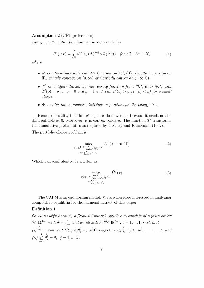
Assumption 2 (CPT-preferences)
Every agent‘s utility function can be represented as
U i(∆x) =∫
IRui(∆y) d ( T i ◦ Φ(∆y)) for all ∆x ∈ X, (1)
where
• ui is a two-times differentiable function on IR \ {0}, strictly increasing onIR, strictly concave on (0,∞) and strictly convex on (−∞, 0),
• T i is a differentiable, non-decreasing function from [0,1] onto [0,1] withT i(p) = p for p = 0 and p = 1 and with T i(p) > p (T i(p) < p) for p small(large),
• Φ denotes the cumulative distribution function for the payoffs ∆x.
Hence, the utility function ui captures loss aversion because it needs not bedifferentiable at 0. Moreover, it is convex-concave. The function T i transformsthe cumulative probabilities as required by Tversky and Kahneman (1992).
The portfolio choice problem is:
maxθ∈ IRJ+1:
∑J
j=0qj θj≤wi
x=∑J
j=0Aj θj
U i(x− βwi1I
)(2)
Which can equivalently be written as:
maxθ∈ IRJ+1:
∑J
j=0qj θj≤wi
x=∑J
j=0Aj θj
U i (x) (3)
The CAPM is an equilibrium model. We are therefore interested in analyzingcompetitive equilibria for the financial market of this paper:
Definition 1
Given a riskfree rate r, a financial market equilibrium consists of a price vector∗q∈ IRJ+1 with
∗q0=
11+r
and an allocation∗θi∈ IRJ+1, i = 1, ..., I, such that
(i)∗θi maximizes U i(
∑j Ajθ
ij − βwi1I) subject to
∑j
∗qj θi
j ≤ wi, i = 1, ..., I, and
(ii)I∑
i=1
∗θi
j = θj, j = 1, ..., J .
7

Note that given the riskfree rate, a financial markets equilibrium determinesthe J prices of the risky assets by clearing the J markets for the risky assets.Instead of analyzing financial markets equilibria as defined in the Definition 1,in the CAPM it is most useful to first transform the decision problem into someabstract problem that uses the structure of the underlying probability space.To do this, note that a necessary condition for the portfolio decision problemgiven above to have a solution is that consumers cannot exploit an arbitrageopportunity. Since the CPT utility U i and hence also the utility U i is strictlyincreasing, this means that the agent cannot find a portfolio that almost surelydelivers positive payoffs without requiring any payments. Asset prices are thusarbitrage free only if the following equation holds:
L2+ ∩
{x ∈ L2 (η)
∣∣∣ x =∑J
j=0 Aj θj where∑J
j=0 qj θj ≤ 0}
= {0} . (4)
Let q ∈ IRJ+1 be an abitrage free price vector. Under Assumption 1, anarbitrage free price vector q needs to satisfy q0 > 0. By the Dalang-Morton-Willinger Theorem (see for example Delbaen 1999), there exists a probabilitymeasure π on (M,M), π ∼ η such that qj
q0= IEπ [Aj] for all j = 1, . . . , J . Here we
consider discounted prices qj
q0. Note that q0 = 1
1+r. We obtain qj = 1
1+rIEπ [Aj].
We can rewrite the pricing rule by defining the Radon-Nikodym Derivative ofπ with respect to η, the so called likelihood ratio process ` = dπ
dη∈ L2(η) and
we obtain qj = 11+r
µ(`Aj) = 11+r
` · Aj. At an equilibrium the price system ` isalso called ’ideal security’ (Magill and Quinzii 1996) or ’pricing portfolio’ (Duffie1988). Applying the pricing rule to the portfolio decision problem recognizingthe way x is generated by θ, delivers the so called no-arbitrage decision problem
maxx∈X
U i (x) , ` · x ≤ (1 + r)wi. (5)
To gain intuition on the Dalang-Merton-Willinger Theorem, we briefly considerthe case for M finite, M = 2|M | and η(m) > 0 for all m ∈ M . The arbitragefree equation (4) implies that
x =
J∑
j=0
Aj θj
∣∣∣∣∣∣
J∑
j=0
qj θj ≤ 0
∩
{h ∈ L2 (η)
∣∣∣∣∣h ≥ 0,∑
m∈M
h(m) = 1
}= ∅.
Let K ={x =
∑Jj=0 Aj θj
∣∣∣ ∑Jj=0 qj θj ≤ 0
}. K defines a sub-space of L2(η). Let
P = {h ∈ L2 (η) |h ≥ 0,∑
m∈M h(m) = 1}. Since K ∩ P = ∅, then by Farka’sLemma we find a linear functional Ψ on L2(η) with Ψ(f) = 0 for f ∈ K andΨ(h) > 0 for h ∈ P . Moreover, by the Riesz Representation Theorem (see Duffie1988, Chapter I.6) we find ψ ∈ L2(η) with Ψ(g) = µ(ψ g) for all g ∈ L2(η). Letm ∈ M and define hm by hm(m′) = 1 if m′ = m and hm(m′) = 0 else. hm is
8

the Arrow security for state m. Obviously hm ∈ P and 0 < Ψ(hm) = ψ(m)η(m)for all m ∈ M . Since η(m) > 0 then ψ(m) > 0. We define ` = ψ
µ(ψ)and a
probability measure π on (M,M) by π(m) = `(m)η(m). We have
µ(ψ)−1Ψ(g) =∑
m∈M
g(m) π(m) = IEπ [g] .
Consider the following investment: Borrow θ0 = −1 units of the riskfree asset,to finance θi = q0
qiunits of asset i ∈ {1, . . . , J} (θk = 0 for k 6= 0, i). Then,
x =∑J
j=0 θj Aj ∈ K and thus µ(ψ)−1Ψ(x) = IEπ [x] = 0. It follows:
qj =q0
IEπ [1I]IEπ [Aj] =
1
1 + rIEπ [Aj] .
Since we restrict the pricing rule just described to X, we can assume withoutloss of generality2 that ` ∈ X. In fact, if ` /∈ X, we can decompose ` into onepart `‖ in X and one part `⊥ orthogonal to X. Since for all x ∈ X, `⊥ · x = 0,the pricing rule can be rewritten as `‖ · x. Thus, we assume ` ∈ X. Back to theno-arbitrage decision problem (5), we can now give an equivalent definition offinancial markets equilibria that is easier to analyze than the Definition 1:
Definition 2
Given a riskfree rate r, a financial market equilibrium consists of a price vector∗` ∈ X and an allocation
∗xi∈ L2(η), i = 1, ..., I, such that (i)
∗xi maximizes U i(x)
subject to x ∈ X and∗` · x ≤ (1 + r) wi, i = 1, ..., I, and (ii)
I∑i=1
∗x
i
⊥= ω.
3 Results
Before we exploit the specific assumptions, Assumption 1 and 2, made in theprevious section we will briefly recall what can already be said with respect toasset prices.
Proposition 1 (Asset Pricing)
Let y be any payoff in X and define q(y) :=∑
j qjθj for some θ with y =∑
j Ajθj.Then we obtain that in any financial market equilibrium the likelihood ratio pro-cess ` is the only risk factor of the model, i.e. q(y) = 1
1+r(µ(y) + cov(y, `)).
2This assumption just refers to the pricing rule ` · x and not to the way ` is obtained. Itmight occur that the new ` cannot be written as Radon-Nikodym Derivative with respect tosome equivalent probability measure.
9
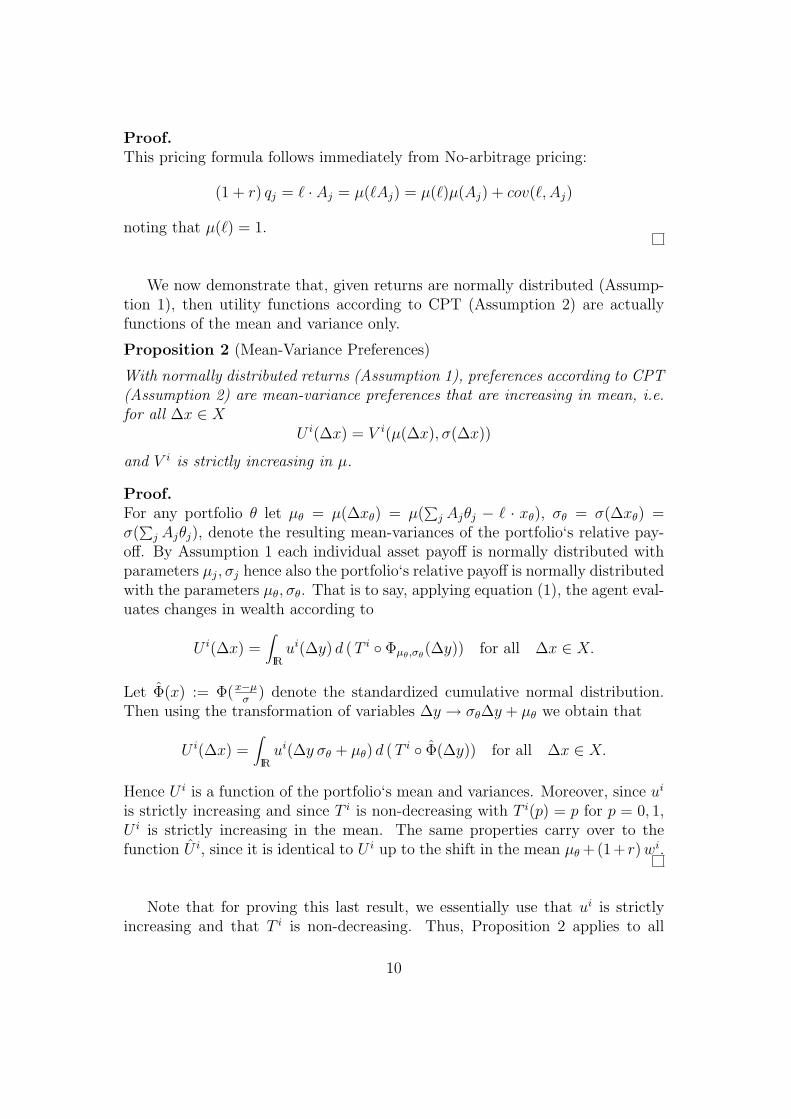
Proof.This pricing formula follows immediately from No-arbitrage pricing:
(1 + r) qj = ` · Aj = µ(`Aj) = µ(`)µ(Aj) + cov(`, Aj)
noting that µ(`) = 1.
We now demonstrate that, given returns are normally distributed (Assump-tion 1), then utility functions according to CPT (Assumption 2) are actuallyfunctions of the mean and variance only.
Proposition 2 (Mean-Variance Preferences)
With normally distributed returns (Assumption 1), preferences according to CPT(Assumption 2) are mean-variance preferences that are increasing in mean, i.e.for all ∆x ∈ X
U i(∆x) = V i(µ(∆x), σ(∆x))
and V i is strictly increasing in µ.
Proof.For any portfolio θ let µθ = µ(∆xθ) = µ(
∑j Ajθj − ` · xθ), σθ = σ(∆xθ) =
σ(∑
j Ajθj), denote the resulting mean-variances of the portfolio‘s relative pay-off. By Assumption 1 each individual asset payoff is normally distributed withparameters µj, σj hence also the portfolio‘s relative payoff is normally distributedwith the parameters µθ, σθ. That is to say, applying equation (1), the agent eval-uates changes in wealth according to
U i(∆x) =∫
IRui(∆y) d ( T i ◦ Φµθ,σθ
(∆y)) for all ∆x ∈ X.
Let Φ(x) := Φ(x−µσ
) denote the standardized cumulative normal distribution.Then using the transformation of variables ∆y → σθ∆y + µθ we obtain that
U i(∆x) =∫
IRui(∆y σθ + µθ) d ( T i ◦ Φ(∆y)) for all ∆x ∈ X.
Hence U i is a function of the portfolio‘s mean and variances. Moreover, since ui
is strictly increasing and since T i is non-decreasing with T i(p) = p for p = 0, 1,U i is strictly increasing in the mean. The same properties carry over to thefunction U i, since it is identical to U i up to the shift in the mean µθ +(1+ r) wi.
Note that for proving this last result, we essentially use that ui is strictlyincreasing and that T i is non-decreasing. Thus, Proposition 2 applies to all
10

utility functions satisfying equation (1) where ui is strictly increasing and T i
non-decreasing with T i(p) = p for p = 0, 1.
The mean-variance property of preferences is the main property to derive theTobin Separation Principle and thus to derive the Mutual Fund Theorem:
Proposition 3 (Tobin Separation)
Let xi ∈ arg maxx∈X U i(x) s.t. ` · x ≤ (1 + r) wi for i = 1, . . . , I and supposethat µ(ω) > ` · ω. Then xi = ψi1I − φi` for some scalars φi ≥ 0, ψi for everyi = 1, ..., I.
Proof.We prove Proposition 3 by the following four steps.
(1) Budget restriction holds with equality.Let xi ∈ arg maxx∈X U i(x) s.t. ` · x ≤ (1 + r) wi. Since there is a riskless assetand since the function U i is increasing in µ, then at any optimal solution xi thebudget restriction holds with equality, i.e. ` · xi = (1 + r) wi for all i. Otherwiseit would be possible to further increase the utility by buying the riskfree asset.
(2) Agents are variance averse.Let xi ∈ arg maxx∈X U i(x) s.t. ` · x ≤ (1 + r) wi and suppose that µ(ω) > ` · ω.
Since µ(ω) > ` · ω, then µ(ω−q(ω)q(ω)
) > r, i.e. the return on the market portfolio isgreater than the risk free return r and thus, if investor i were not variance averseat xi, she would then short sell the risk free asset and buy the market portfolio,increasing in this way her utility and contradicting the optimality of xi.
(3) Tobin’s Separation.Let xi ∈ arg maxx∈X U i(x) s.t. ` · x ≤ (1 + r) wi and suppose that µ(ω) > ` · ω.Decompose xi = yi+zi where zi is perpendicular to 1I and ` and yi ∈ span(1I, `) ⊂X. From the decomposition it follows that ` · zi = 0 so that yi ∈ X is budgetfeasible. Moreover, from zi being perpendicular to 1I it is obtained that µ(xi) =µ(yi). Suppose that zi 6= 0, then
σ2(xi) = σ2(xi⊥) = ‖xi
⊥‖2 = ‖yi⊥ + zi
⊥‖2 = ‖yi⊥‖2 + ‖zi
⊥‖2
> ‖yi⊥‖+ ‖zi
⊥‖2 = σ2(yi⊥) = σ2(yi)
because zi⊥ is perpendicular to yi
⊥, where the subscript ⊥ denotes the componentof each vector orthogonal to 1I. Since by (2) investors are variance averse at theoptimal allocation xi, then zi = 0. Therefore xi = ψi1I − φi` for some scalarsφi, ψi for every i = 1, ..., I, i.e. Tobin’s Separation holds.
11

(4) φi ≥ 0 .From (3) we obtain xi = ψi1I − φi`. It remains to show that φi ≥ 0. Fromxi = ψi1I − φi` and the budget equality ` · xi = (1 + r) wi, it follows µ(xi) =(1+r) wi + φiσ2(`) and σ(xi) = |φi|σ(l). If φi < 0, then, because by Proposition2 V i is increasing in µ one could increase the utility by buying the asset ψi1I+φi`,a contradiction to the optimality of xi.
The next result shows that without loss of generality we can work in thefamous mean-variance diagram.
Corollary 1 (Mean-Variance Principle)
Suppose that µ(ω) > ` · ω, then the decision problems
xi ∈ arg maxx∈X
U i(x) s.t. ` · x ≤ (1 + r) wi
and
(µi, σi) ∈ arg max(µ,σ)∈IR×IR+
V i(µ− (1 + r) wi, σ) s.t. µ− qσ = (1 + r) wi
are equivalent, where q = σ(`) > 0.
Proof.¿From step (4) of the proof of Proposition 3 we obtain µ(xi) = (1 + r) wi +σ(xi) σ(`) for any optimal solution xi of the first decision problem. Moreover, byProposition 2, (µ(xi), σ(xi)) maximizes V i. On the other hand, for any solution(µi, σi) of the second decision problem we can find unique ψi and Φi ≥ 0 suchthat xi = ψi1I− φi` has mean µi and variance σi. ¿From the budget restrictionof the second decision problem, it follows that xi is budget feasible for investori. Moreover, by Proposition 2, xi maximizes U i.
Now we are in a position to consider the equilibrium consequences of whatwe discovered so far:
Proposition 4 (Mutual Fund Theorem)
Given a riskfree rate r, let (∗`,∗x) with
∗x = (
∗x
1, ...,
∗x
I) be a financial market
equilibrium and suppose µ(ω) >∗` ·ω. Then there exist scalars φi ∈ IR+, i =
0, 1, ..., I , and scalars ψi ∈ IR, i = 0, 1, ..., I such that∗` = ψ01I + φ0ω and
∗x
i= ψi1I− φiω for every i = 1, ..., I.
12

Proof.By Tobin’s Separation (Proposition 3)
∗x
i= ψi1I− φi
∗` for some scalars φi ≥ 0, ψi
for every i = 1, ..., I. Since in equilibrium∑
i
∗x
i
⊥= ω⊥ we get∑
i
∗x
i= α1I + ω
for some α ∈ IR. Hence there exist scalars φ0 ≥ 0, ψ0 such that∗`= ψ01I − φ0ω.
Using this last equation, we obtain∗x
i= ψi1I−φiω for some scalars φi ≥ 0, ψi for
every i = 1, ..., I.
The main conclusion of the CAPM, the Security Market Line Theorem, isnow straightforward:
Proposition 5 (Security Market Line Theorem)
Suppose that the gross return of the market portfolio is greater than the risk free
gross return, i.e. µ(ω) >∗` ·ω. Then, given asset payoffs are normally distributed
(Assumption 1) and agents have prospect theory utility functions (Assumption
2), at every financial market equilibrium (∗`,∗x) the security market line holds,
i.e. for any payoff y ∈ X
µ(ry)− r =cov(ry, rω)
σ2(rω)(µ(rω)− r) (6)
where ry = y−q(y)q(y)
and rω = ω−q(ω)q(ω)
.
Proof.Inserting the Mutual Fund Theorem expression for
∗` = ψ01I−φ0ω into the asset
pricing formula derived in Proposition 1, gives:
(1 + r)q(y) = µ(y)− φ0cov(ω, y).
Applying this formula for y = ω we can determine φ0 > 0 as
φ0 =µ(ω)− (1 + r) q(ω)
σ2(ω).
Hence we obtain:
(1 + r)q(y) = µ(y)− µ(ω)− (1 + r)q(ω)
σ2(ω)cov(ω, y),
which can also be written as
(1 + r) q(y)− µ(y) =cov(ω, y)
σ2(ω)((1 + r)q(ω)− µ(ω)) .
13
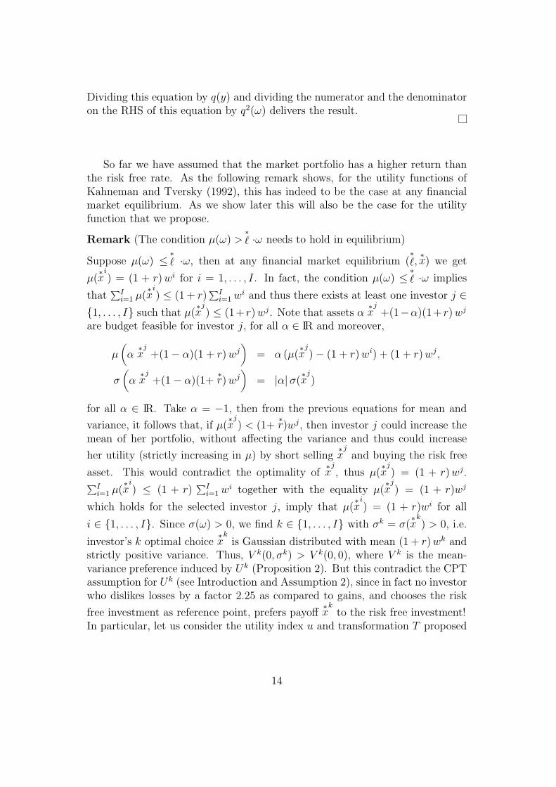
Dividing this equation by q(y) and dividing the numerator and the denominatoron the RHS of this equation by q2(ω) delivers the result.
So far we have assumed that the market portfolio has a higher return thanthe risk free rate. As the following remark shows, for the utility functions ofKahneman and Tversky (1992), this has indeed to be the case at any financialmarket equilibrium. As we show later this will also be the case for the utilityfunction that we propose.
Remark (The condition µ(ω) >∗` ·ω needs to hold in equilibrium)
Suppose µ(ω) ≤ ∗` ·ω, then at any financial market equilibrium (
∗`,∗x) we get
µ(∗x
i) = (1 + r) wi for i = 1, . . . , I. In fact, the condition µ(ω) ≤ ∗
` ·ω implies
that∑I
i=1 µ(∗x
i) ≤ (1 + r)
∑Ii=1 wi and thus there exists at least one investor j ∈
{1, . . . , I} such that µ(∗x
j) ≤ (1+ r) wj. Note that assets α
∗x
j+(1−α)(1+ r) wj
are budget feasible for investor j, for all α ∈ IR and moreover,
µ(α
∗x
j+(1− α)(1 + r) wj
)= α (µ(
∗x
j)− (1 + r) wi) + (1 + r) wj,
σ(α
∗x
j+(1− α)(1+
∗r) wj
)= |α| σ(
∗x
j)
for all α ∈ IR. Take α = −1, then from the previous equations for mean and
variance, it follows that, if µ(∗x
j) < (1+
∗r)wj, then investor j could increase the
mean of her portfolio, without affecting the variance and thus could increase
her utility (strictly increasing in µ) by short selling∗x
jand buying the risk free
asset. This would contradict the optimality of∗x
j, thus µ(
∗x
j) = (1 + r) wj.
∑Ii=1 µ(
∗x
i) ≤ (1 + r)
∑Ii=1 wi together with the equality µ(
∗x
j) = (1 + r)wj
which holds for the selected investor j, imply that µ(∗x
i) = (1 + r)wi for all
i ∈ {1, . . . , I}. Since σ(ω) > 0, we find k ∈ {1, . . . , I} with σk = σ(∗x
k) > 0, i.e.
investor’s k optimal choice∗x
kis Gaussian distributed with mean (1 + r) wk and
strictly positive variance. Thus, V k(0, σk) > V k(0, 0), where V k is the mean-variance preference induced by Uk (Proposition 2). But this contradict the CPTassumption for Uk (see Introduction and Assumption 2), since in fact no investorwho dislikes losses by a factor 2.25 as compared to gains, and chooses the risk
free investment as reference point, prefers payoff∗x
kto the risk free investment!
In particular, let us consider the utility index u and transformation T proposed
14

by Tversky and Kahneman (1992):
u(x) =
{xα for x ≥ 0,
−λ(−x)β for x < 0,(7)
T (p) =pγ
(pγ + (1− p)γ)1γ
. (8)
where β = α = 0.88, λ = 2.25 and γ = 0.61 for gains and γ = 0.69 for losses.The induced mean-variance preference V k satisfies V k(0, σ) = c σα for all σ ≥ 0,where c ≈ −0.34. Therefore V k(0, σ) < V k(0, 0) for all σ > 0, i.e. no investorwill choose a positive variance.In summary, this remark has shown that the existence of financial market equi-libria for the case µ(ω) ≤ ` · ω is not consistent with Tversky and Kahneman(1992) assumptions for the utility functions.
4 Existence of Equilibria
Up to now we have assumed that a financial market equilibrium exists. This as-sumption implies that each investor’s decision problem has a solution (Definition1 and 2). The no arbitrage condition expressed by equation (4), is a necessarycondition for the existence of a solution of the investor’s decision problem, butit is not sufficient. To understand why the investor‘s decision problem may failto have a solution, let us consider the following general example.
Suppose Assumptions 1 and 2 are satisfied and the no arbitrage condition(4) holds. Let ` be the pricing portfolio. We suppose, as in Proposition 3, 4 and
5, that µ(ω) > ` · ω and we define δ(ω) = µ(ω)−`·ωσ(ω)
. Note that δ(ω) corresponds
the the Sharpe Ratio of the market portfolio µ(rω)−rσ(rω)
(Sharpe 1994). Let ω =
(1 + r) wk
`·ω ω. Then ω is budget feasible for investor k and δ(ω) = δ(ω) > 0. Weconsider the leveraged portfolio x(α) = α ω + (1− α)(` · ω) 1I. Then
` · x(α) = ` · ω,
µ (x(α)) = α (µ(ω)− ` · ω) + ` · ω,
i.e. x(α) is budget feasible and µ (x(α)) ↗∞ as α ↗∞.
Suppose, for sake of simplicity, that investor k does not transform the distri-bution function, i.e. T k(p) = p for all p ∈ [0, 1] and uses the utility index
uk(x) =
f(x) for x > 0;0 for x = 0;−λ f(−x) for x < 0,
15

where f(x) = x is the linear function on (0,∞) and λ ≈ 2.25 (see Barberis,Huang and Santos 2001). We consider the utility function Uk on the set {x(α) |α >0}. We have:
V k(α) = Uk(x(α)) = V k(α µ(ω)− α ` · ω, ασ(ω))
=∫
IRuk (α(σ(ω)x + µ(ω)− ` · ω)) dΦ(x)
= α
[∫ ∞
−δ(ω)(σ(ω) x + µ(ω)− ` · ω) dΦ(x)
+∫ −δ(ω)
−∞λ (σ(ω) x + µ(ω)− ` · ω) dΦ(x)
]
= α[(µ(ω)− ` · ω)
(1 + (λ− 1) Φ(−δ(ω))
)+ σ(ω) (λ− 1) ϕ(δ(ω))
]
= α c(λ, δ(ω)).
where ϕ is the probability density of the standard normal distribution. For theU.S. economy, Mehra (2003) gives an estimate of the long-term Sharpe Ratio ofδ(ω) = 0.34 and c(2.25, 0.34) > 0. Thus investor k can infinitely increase herutility by infinitely leveraging the market portfolio and therefore no solution toher decision problem would exist.
Tversky and Kahnemann (1992).We restrict now our attention to the utility index and probability transformationproposed by Tversky and Kahnemann, which are defined in equations (7) and(8). For the reasoning of this subsection it will be important to allow for somepossibly small heterogeneity in agents preferences. Therefore let:
ui(x) =
{xαi
for x ≥ 0,
−λi(−x)αifor x < 0,
(9)
T i(p) =pγi
(pγi + (1− p)γi
) 1
γi
. (10)
The Corollary 1 to the Tobin’s Separation Theorem implies that for anypricing portfolio ` with µ(ω) > ` · ω, xi solves
maxx∈X
U i(x) s.t. ` · x ≤ (1 + r) wi
iff (µ(xi), σ(xi)) solves
max(µ,σ)∈IR×IR+
V i(µ− (1 + r) wi, σ) s.t. µ− qσ = (1 + r) wi,
16

where q = σ(l) > 0. We consider U i(xi) = V i(qσ, σ) induced by (7) and (8). Weobtain:
V i(qσ, σ) = σαi[∫ ∞
−q(x + q)αi
d(T i ◦ Φ(x))− λi∫ −q
−∞(−x− q)αi
d(T i ◦ Φ(x))]
= σαi
f i(q),
where f i(q) =[∫∞−q(x + q)αi
d(T i ◦ Φ(x))− λi∫−q−∞(−x− q)αi
d(T i ◦ Φ(x))]is con-
tinuous and strictly increasing on IR+, f i(0) ≈ −0.34 and f i(q) ↗∞ as q ↗∞.Thus for all agents i = 1, . . . , I, there exists exactly one qi > 0 such thatf i(qi) = 0. It follows that for 0 < q < qi, investor i’s optimal allocation is therisk free asset, for q = qi the investor is indifferent between all possible alloca-tions and for q > qi investor i’s optimal behavior consists in infinitely leveragingthe market portfolio. Thus as soon as the investors are a little heterogenousno equilibrium exists. Figure 2 shows the Tversky and Kahnemann indifferencecurves in the (σ, µ) plane. For all pricing portfolios ` such that q 6= qi, nosolution to the individual optimization problem can exists under Tversky andKahneman’s (1992) assumptions for the utility functions.
Our proposal.We suggest to consider the following utility index
u(x) =
{−λ+ exp(−α x) + λ+ for x ≥ 0,
λ− exp(α x)− λ− for x < 0,(11)
where α ∈ (0, 1), λ− > λ+ > 0. Figure 1 shows that u(x) approximates theTversky and Kahnemann (1992) utility index very well for values around zero.We presume that the experimental evidence given for the utility specificationof Kahneman and Tversky (1979) foremost concerns the shape of the utilityfunction around zero. Note also that the utility function we propose is differentto that of Kahneman and Tversky (1979) for very high stakes because it isless linear than theirs. Our theoretical analysis thus suggest to conduct furtherexperiments in this direction. For sake of simplicity we take T (p) = p for allp ∈ [0, 1]. As it will be seen later for this specification financial markets equilibriaare robust with respect to introducing some heterogeneity of agents’ preferences.For any agent at any consumption bundle, x ∈ X, µ(∆x) = µ, σ(∆x) = σ weobtain (see Appendix):
U(∆x) = V (µ, σ) =∫
IRu(σ∆y + µ) dΦ(∆y)
= (λ+ + λ−)Φ(
µ
σ
)− λ−
+ e12σ2α2
[λ− eαµ Φ
(−µ
σ− ασ
)− λ+ e−αµ Φ
(µ
σ− α σ
)].
17

Figure 3 shows the indifference curves of V in the mean and standard deviationspace. The partial derivatives of V are
∂µV (µ, σ) = α e12α2σ2
[λ− eαµ Φ
(−µ
σ− ασ
)+ λ+ e−αµ Φ
(µ
σ− ασ
)],
∂σV (µ, σ) = α2 σ e12α2σ2
[λ− eαµ Φ
(−µ
σ− ασ
)− λ+ e−αµ Φ
(µ
σ− ασ
)]
−α (λ− − λ+) ϕ(
µ
σ
).
where ϕ = Φ′ is the density function for the standard normal distribution. Theratio
S(µ, σ) = −∂σV (µ, σ)
∂µV (µ, σ)
gives the slope of the indifference curve at some point in the mean and standarddeviation space. The following properties hold:
(i) ∂µV (µ, σ) > 0,
(ii) ∂σV (µ, 0) = 0, ∂σV (µ, σ) < 0 for σ > 0 3
and limσ→∞ ∂σV (µ, σ) = 0 for all µ > 0,
(iii) S(µ, 0) = 0 and S(µ, σ) > 0 for all µ > 0,
(iv) limµσ→∞ S(µ, σ) = α σ for all σ > 0 fix,
(v) limσ→∞ S(µ, σ) = ∞ for all µ > 0.
The proof is given in the Appendix. Note that property (ii) implies that the
condition µ(ω) >∗` ·ω needs to hold in equilibrium also under our proposal for
the utility index. In fact, as we have already shown in the Remark in the pre-
vious section, µ(ω) ≤ ∗` ·ω holds in equilibrium only if some investor’s optimal
allocation is a risky investment with same return as the risk-free asset, a contra-diction to property (ii).The final property we need to show is the quasi-concavity of V . Tobin (1958) has
3Property 2 expressed in Meyer (1987) states that when the class of considered risks isgenerated by a location and scale parameter condition, then for V given by (1), ∂σV (µ, σ) ≤ 0if and only if the utility index u satisfies u′′(µ + σ x) ≤ 0 for all µ + σ x. Since the utilityindex (11) does not satisfy u′′(µ + σ x) ≤ 0 for all µ + σ x, one could expect our statementto contradict Property 2 in Meyer (1987). But this is not the case, since the necessity of thecondition on u for Property 2 in Meyer (1987) holds, if and only if all considered risks havebounded support, which is obviously not the case under the normal distribution assumption.Indeed, our example shows that the necessity condition does not hold for risks with unboundedsupport.
18

already pointed out that quasi-concavity of the mean-variance utility functionV is ultimately linked to the concavity of the von Neumann-Morgenstern util-ity function u. Indeed, as Sinn (1983) has shown, concavity of u easily impliesquasi-concavity of V . In the case of prospect theory u is however convex-concave.Hence, quasi-concavity of V depends on whether on average the distribution of∆x puts more weight on the convex or on the concave part of u. The condi-
tion µ(ω) >∗` ·ω, which needs to hold in equilibrium as shown above, ensures
that equilibrium allocation on average have positive excess return. Note alsothat loss-aversion, i.e. the feature that u is steeper for losses than for gains,contributes to the concavity of u and hence to the quasi-concavity of V . In-deed, it turns out that our choice of the parameters λ+, λ− and α leads to aquasi-concave utility function V (see Figure 3). This puts us into the positionof proving our final claim:
Proposition 5 (Existence of CAPM-equilibria)
Under the assumptions (1) and (2) and for the specification of the CPT-utilityfunctions given by (9), for any given riskfree rate r, there exist financial market
equilibria with µ(ω) >∗` ·ω.
Proof.Consider the standard deviation of the market portfolio, σ(ω). by the mean-
variance-principle (Corollary 1), we need to find a price∗q such that
∑i σ
i(∗q) =
σ(ω), whereσi ∈ arg max
σ∈IR+
V i(qσ, σ).
From the boundary behavior of the agents indifference curves (i) to (v) that weshowed above, it follows for all i = 1, . . . , I that for q → 0 σi(q) = 0 and forq →∞ σi(q) = ∞. Hence for sufficiently small prices of risk, q, market demand∑
i σi(∗q) is smaller than market supply σ(ω) while for sufficiently large prices it
is larger. Since by the quasi-concavity of preferences demand is continuous, fromthe intermediate value theorem we get the existence of some equilibrium with∗q > 0. Finally, note that
∗q > 0 is equivalent to µ(ω) >
∗` ·ω.
5 Conclusion
Under the assumption of normally distributed returns, we have shown that theCumulative Prospect Theory of Tversky and Kahneman (1992) is consistent
19
with the Capital Asset Pricing Model in the sense that in every financial marketequilibrium the Security Market Line Theorem holds. However, we did also showthat under the specific functional forms suggested by Tversky and Kahneman(1992) financial market equilibria do not exist. We suggested an alternativefunctional form consistent with the results of Tversky and Kahneman for whichequilibria do exist.
The functional form we suggest differs from that of Kahneman and Tversky(1979) with respect to the behavior for large stakes. This suggests to collectexperimental evidence with large stakes since for the existence of equilibria thebehavior of agents at the boundary of their consumption space is essential.
The CAPM analyzed in this paper is a standard two periods model. Whilemuch of the intuition for the general intertemporal CAPM can already be givenin the two periods model still it would be very interesting to check the consistencyof prospect theory and the CAPM also in the intertemporal model. In particularit is unclear whether the intertemporal CAPM is consistent with possible shiftsin the reference point. Moreover, in the intertemporal model returns will be en-dogenous and most likely not normally distributed, giving prospect theory somechance to differ from mean-variance analysis. For recent papers incorporatingsome aspects of prospect theory in intertemporal models see Benartzi and Thaler(1995) and also Barberis, Huang and Santos (2001).
References
Allais, M. (1953) : “Le Comportement de l‘Homme Rationnel devant le Risque:Critique des Postulates et Axiomes de l‘Ecole Americaine”, Econometrica,21, 503–546.
Barberis, N., Huang, M. and T. Santos (2001) : “Prospect Theory andAsset Prices”, Quarterly Journal of Economics, 116, 1–53.
Benartzi, S. and R. Thaler (1999) : “Myopic Loss Aversion and the EquityPremium Puzzle”, Quarterly Journal of Economics, 110, 75–92.
De Bondt, W. (1999) : “Behavioural Economics, A Portrait of the IndividualInvestor”, European Economic Review, 42, 831–844.
Bossaert, P. (2002) : The Paradox of Asset Pricing, Princeton UniversityPress.
Copeland, T.E. and J.F. Weston, (1998) : Financial Theory and Corpo-rate Policy, Addison Wesley, 3rd edition.
20

Delbaen, F. (1999) : “The Dalang-Morton-Willinger Theorem”, Unpublishednote, ETH Zurich, available from “ http://www.math.ethz.ch/∼delbaen”.
Duffie, D. (1988) : Security Markets: Stochastic Models, Academic Press.
Ellsberg, D. (1961) : “Risk, Ambiguity, and the Savage Axioms”, QuarterlyJournal of Economics, 75, 643-669.
Jagannathan, R. and Z. Wang (1996) : “The Conditional CAPM and theCross-Section of Expected Returns”, Journal of Finance, 51, 3–53.
Kahneman, D. and A. Tversky (1979) : “Prospect Theory: An Analysisof Decisions Under Risk”, Econometrica, 47, 263-291.
Lintner, J. (1965) : “The Valuation of Risky Assets and the Selection of RiskyInvestment in Stock Portfolios and Capital Budgets”, Review of Economicsand Statistics, 47, 13–37.
Levy, H., De Giorgi, E. and T. Hens (2003) : “Two Paradigms and No-bel Prizes in Economics: a Contradiction or Coexistence?”, NCCR-FinriskWorking Paper No. ??, University of Zurich.
Benartzi, S. and R. Thaler (1999) : “Myopic Loss Aversion and the EquityPremium Puzzle”, Quarterly Journal of Economics, 110, 75–92.
Magill, M. and M. Quinzii (1996) : The Theory Of Incomplete Markets,Volume 1, MIT-Press.
Markowitz, H.M. (1952) : “Portfolio Selection”, Journal of Finance, 7, 77-91.
Mehra, R. (2003) : “The Equity Premium: What is the Puzzle?”, FinancialAnalyst Journal, January-February, 59–64.
Meyer, J. (1987) : “Two-Moment Decision Models and Expected Utility Max-imization”, The American Economic Review, 77, 421–430.
Mossin, J. (1966) : “Equilibrium in a Capital Asset Market”, Econometrica,34, 768–783.
Savage, L.(1954) : The Foundations of Statistics, Wiley.
Sharpe, W. (1964) : “Capital Asset Prices: A Theory of Market EquilibriumUnder Conditions of Risk”, Journal of Finance, 19, 425–442.
– (1994) : “The Sharpe Ratio”, Journal of Portfolio Management, 21, 49–59.
21
Sinn, H.W. (1983) : Economic Decisions under Uncertainty, Amsterdam,North-Holland.
Tobin, J. (1958) : “Liquidity Preference as Behavior Towards Risk”, ReviewEcononic Studies, 25, 65–86.
Tversky, A. and D. Kahneman (1992) : “Advances in Prospect Theory:Cumulative Representation of Uncertainty”, Journal of Risk and Uncer-tainty, 5, 297–323.
von Neumann, J. and O. Morgenstern (1944) : The Theory of Games andEconomic Behavior, Princeton University Press.
22

Appendix
First we prove that
(0)
V (µ, σ) = (λ+ + λ−)Φ(
µ
σ
)− λ−
+ e12σ2α2
[λ− eαµ Φ
(−µ
σ− ασ
)− λ+ e−αµ Φ
(µ
σ− α σ
)],
if
u(x) =
{−λ+ exp(−α x) + λ+ for x ≥ 0,
λ− exp(α x)− λ− for x < 0,(12)
where α ∈ (0, 1), λ− > λ+ > 0.
(i) ∂µV (µ, σ) > 0,
(ii) ∂σV (µ, 0) = 0, ∂σV (µ, σ) < 0 for σ > 0 and limσ→∞ ∂σV (µ, σ) = 0 for allµ > 0,
(iii) S(µ, 0) = 0 and S(µ, σ) > 0 for all µ > 0,
(iv) limµσ→∞ S(µ, σ) = α σ for all σ > 0 fix,
(v) limσ→∞ S(µ, σ) = ∞ for all µ > 0.
Proof.(0)
U(∆x) = V (µ, σ) =∫
IRu(σ∆y + µ) dΦ(∆y)
=∫ ∞
−µσ
(−λ+e−α(σx+µ) + λ+
)dΦ(x) +
∫ −µσ
−∞
(λ−eα(σx+µ) − λ−
)dΦ(x)
= λ+(1− Φ
(−µ
σ
))− λ− Φ
(−µ
σ
)+
+ λ− eα µ∫ −µ
σ
−∞eασx dΦ(x)− λ+ e−α µ
∫ ∞
−µσ
e−ασx dΦ(x)
= (λ+ − λ−) Φ(
µ
σ
)− λ− +
+ λ− eα µ∫ ∞
µσ
e−ασx dΦ(x)− λ+ e−α µ∫ ∞
−µσ
e−ασx dΦ(x)
= (λ+ − λ−) Φ(
µ
σ
)− λ− +
+ e12α2σ2
[λ− eα µ Φ
(−µ
σ− ασ
)− λ+ e−α µ Φ
(µ
σ− ασ
)].
23

For the last equality, we use that∫∞z e−ασx dΦ(x) = e
12α2σ2
Φ (−ασ − z).
(i)From (0) we obtain
∂µV (µ, σ) = α e12α2σ2
[λ− eαµ Φ
(−µ
σ− ασ
)+ λ+ e−αµ Φ
(µ
σ− ασ
)],
thus ∂µV (µ, σ) > 0 for all µ and σ.
(ii)From (0) we obtain
∂σV (µ, σ) = α2 σ e12α2σ2
[λ− eαµ Φ
(−µ
σ− ασ
)− λ+ e−αµ Φ
(µ
σ− ασ
)]
−α (λ− − λ+) ϕ(
µ
σ
).
It follows:
• ∂σV (µ, 0) = 0, using that Φ(−∞) = 0, Φ(∞) = 1 and ϕ(∞) = 0.
• Let us consider f(µ, σ) = σ−1 e−12α2σ2
e−α µ ∂σV (µ, σ) for σ > 0 . We showthat f(µ, σ) < 0.Suppose that for some µ? and σ(µ?) > 0, f(µ, σ(µ?)) > 0. Since f(µ, ·)is continuous, limσ→0 f(µ, σ) = −λ+ e−2 α µ < 0 and limσ→∞ f(µ, σ) = 0for all µ > 0, we can assume without loss of generality that σ(µ?) > 0 isa local maxima of f(µ?, ·). We compute the partial derivative of f withrespect to σ. We have
∂σf(µ, σ) = ϕ(
µ
σ+ ασ
) [λ−(µσ−2 − α) + λ+(µσ−2 + α)
−α−1 (λ− − λ+)(µ2σ−4 − α2 − σ−2
)]
Let η = σ−2, then
∂σf(µ, σ) = 0 ⇔ η
[−λ− − λ+
αµ2 η + (λ− + λ+) µ +
(λ− − λ+)
α
]= 0
⇔ η ∈ {0, η?(µ)}where η?(µ) = α µ (λ−+λ+)+(λ−−λ+)
(λ−−λ+) µ2 . Moreover, for η > η?(µ), ∂σf(µ, σ) < 0
and for 0 < η < η?(µ), ∂σf(µ, σ) > 0. It follows that σ?(µ) = η?(µ)−1/2 > 0is the unique (local) maximum/minimun of f(µ, ·) and since for σ > σ?(µ),∂σf(µ, σ) > 0 and for 0 < σ < σ?(µ), ∂σf(µ, σ) < 0, σ?(µ) is a minimum.This contradicts the existence of µ? and σ(µ?) local maxima of f(µ?, ·) suchthat f(µ?, σ(µ?)) > 0. Hence, f(µ, σ) < 0 and therefore ∂σV (µ, σ) < 0.
24

• limσ→∞ ∂σV (µ, σ) = 0 for µ > 0 since limσ→∞(σ e
12σ2α2
eαµ Φ(−µσ− ασ)
)=
limσ→∞(σ e
12σ2α2
e−αµ Φ(µσ− ασ)
)= 1
α√
2 πand limσ→∞ ϕ(µ
σ) = 1√
2 π.
(iii)Follows directly from (i) and (ii).
(iv)
S(µ, σ) = −∂σV (µ, σ)
∂µV (µ, σ)
= −α2 σ e
12α2σ2
[λ− eαµ Φ
(−µ
σ− ασ
)− λ+ e−αµ Φ
(µσ− ασ
)]
α e12α2σ2
[λ− eαµ Φ
(−µ
σ− ασ
)+ λ+ e−αµ Φ
(µσ− ασ
)]
+α (λ− − λ+) ϕ
(µσ
)
α e12α2σ2
[λ− eαµ Φ
(−µ
σ− ασ
)+ λ+ e−αµ Φ
(µσ− ασ
)]
= −α σ
[λ−
Φ(−µσ−ασ)
Φ(µσ−ασ)
− λ+ e−2 αµ
]
λ−Φ(−µ
σ−ασ)
Φ(µσ−ασ)
+ λ+ e−2 αµ
+(λ− − λ+)
ϕ(µσ
+α σ)Φ(µ
σ−ασ)
λ−Φ(−µ
σ−ασ)
Φ(µσ−ασ)
+ λ+ e−2 αµ
.
For µσ
fix, we have
limσ→∞
Φ(−µ
σ− ασ
)
Φ(
µσ− ασ
) = e−2 αµ,
limσ→∞
ϕ(
µσ
+ α σ)
Φ(
µσ− ασ
) = e−2 αµ limσ→∞
(µ σ + α σ3)(−µ + α σ2)
µ + α σ2.
and thus
limσ→∞S(µ, σ) =
λ− − λ+
λ− + λ+lim
σ→∞
(−α σ +
(µσ + α σ3)(−µ + α σ2)
µ + α σ2
)= ∞.
(v)Let consider the equation for S given above. For σ fix, we have
limµσ→∞
Φ(−µ
σ− ασ
)
Φ(
µσ− ασ
) = 0,
limµσ→∞
ϕ(
µσ
+ α σ)
Φ(
µσ− ασ
) = 0.
25

and thus
limµσ→∞
S(µ, σ) = α σ.
26

-10 -5 0 5 10
x
-15
-10
-50
5
y1
Figure 1: Tversky and Kahneman (1992) utility index (full line) and u(x) =−λ+ e−αx + λ+ for x ≥ 0 and u(x) = λ− eαx − λ− for x < 0 (dotted line), whereλ+ = 6.52, λ− = 14.7 and α ≈ 0.2.
27

0.0 0.1 0.2 0.3 0.4 0.5
sigma
0.00
0.05
0.10
0.15
0.20
0.25
mu
-0.15-0.1-0.05
0
0.05
0.05
0.05
0.05 0.10.1
0.15
Figure 2: Indifference curves in the mean and standard deviation space for theutility function induced by Tversky and Kahnemann (1992) utility index andprobability transformation.
28

0 5 10 15 20
sigma
05
1015
20
mu
-3-2.5-2-1.5-1-0.5
0
0.5
1
1.5
2
2.5
3
3.544.555.56
Figure 3: Indifference curves in the mean and standard deviation space forthe utility function induced by u(x) = −λ+ e−αx + λ+ for x ≥ 0 and u(x) =λ− eαx − λ− for x < 0 where λ+ = 6.52, λ− = 14.7 and α ≈ 0.2.
29