October 8, 2004

ERRATA

This manuscript was submitted to Earthquake Spectra in 1995 for a special issue on the EPRI (1993)

study on strong round motions in the CEUS. The issue was never completed. We are currently updating

this manuscript with analyses for motions recorded by the Port Island vertical array recording from the M

6.9 Kobe Earthquake, adding SHAKE results for all the analyses, and updating the text to reflect similar

work done subsequent to 1995. Comments are welcome (pacificengineering@juno.com).

Reference: Electric Power Research Institute (1993). "Guidelines for determining design basis ground motions." Palo Alto, Calif: Electric Power Research Institute, vol. 1-5, EPRI TR-102293.

vol. 1: Methodology and guidelines for estimating earthquake ground motion in eastern North America.

vol. 2: Appendices for ground motion estimation. vol. 3: Appendices for field investigations. vol. 4: Appendices for laboratory investigations. vol. 5: Quantification of seismic source effects.

1

submitted to Earthquake Spectra

spectra1.tex:February 19, 1995

VALIDATION OF ONE-DIMENSIONAL SITE RESPONSE METHODOLOGIES

Walter Silva, Cathy Stark, Robert Pyke, I.M. Idriss, and James R. Humphrey

Introduction The effects of a soil column upon strong ground motion have been well documented and studied

analytically for many years. Wood (1908) and Reid (1910), using apparent intensity of shaking and

distribution of damage from the 1906 San Francisco earthquake, gave evidence that the severity of

shaking can be substantially affected by the local geology and soil conditions. Gutenberg (1957)

developed amplification factors representing different site geology by examining recordings of

microseisms and earthquakes from instruments located on various types of site geology. More recently,

Wiggins (1964), Idriss and Seed (1968), Seed and Idriss (1969), Borcherdt and Gibbs (1976), Joyner et al.

(1976), Berrill (1977), Duke and Mal (1978), Chin and Aki (1991), Darragh and Shakal (1991), Silva

(1991), Hartzell (1992), Silva and Stark (1992), and Su et al. (1992) have shown that during small and

large earthquakes, the surface soil motion can differ in significant and predictable ways from that on

adjacent rock outcrops. Other investigators have utilized explosion data either independently or in

conjunction with earthquake data to examine site response characteristics (Murphy et al., 1971; Hays et

al., 1979; Rogers et al., 1984). Recent work using horizontal as well as vertical arrays of instruments

have demonstrated the general consistency of the site response for seismic events of different sizes,

distances, and azimuths (Tucker and King, 1984; Benites et al., 1985; Hutchins and Wu, 1990; Chin and

Aki, 1991; Borcherdt and Glassmoyer, 1992; Field et al., 1992; Su et al., 1992; Ditarka et al., 1994; Satoh

etal., 1995; Elgamal et al., 1996; Ganev et al., 1997; Kokusho and Matsumoto, 1997; Dimitriu et al.,

1998). Results of these and other studies have demonstrated, in a general sense, the adequacy of

assuming plane-wave propagation in modeling one-dimensional site response for engineering purposes.

2

Wave Propagation Modeling

In addition to the wave propagation model used in site response analyses, dynamic material properties

such as shear modulus and material damping control the amplitude and frequency content of computed

motions. It is well known from laboratory testing that soils (and indeed soft rocks) exhibit pronounced

nonlinear behavior under shear loading conditions. Shear modulus decreases with increasing strain with

an accompanying increase in material damping (decrease in Qs) (Drnevich et al., 1966; Seed and Idriss,

1970; Hardin and Drnevich, 1972; Seed et al., 1984). If this observation is applicable to in situ-soil

properties subject to earthquake loading, then site response calculations must accommodate these strain

dependencies as nonlinear constitutive relations. In general two approaches are conventionally used to

model cyclic soil response: nonlinear and equivalent-linear.

Nonlinear Model. The two main components of nonlinear analyses are a solution (integration) scheme

for the wave equation and a nonlinear soil model. Nonlinear wave propagation techniques utilize finite

element schemes (Day, 1979), implicit or explicit finite difference schemes (Joyner and Chen, 1975;

Martin, 1975), or the method of characteristics (Streeter et al., 1974). One approach incorporates a

general nonlinear soil model into an explicit finite difference approach which retains second order terms

(Valera et al., 1978; Moriwaki et al., 1981).

Nonlinear soil models which have been primarily developed from laboratory test results and utilized in

dynamic analyses, include the Ramberg-Osgood model (Faccioli et al., 1973; Streeter et al., 1974), an

elasto-plastic model (Richart, 1975), Iwan-type model (Joyner and Chen, 1975; Taylor and Larkin, 1978;

Valera et al., 1978), the hyperbolic model (Hardin and Drnevich, 1972), the endochronoic model (Day,

1979), and the Davidenkov model (Martin, 1975; Pyke, 1979).

Each of the nonlinear models mentioned has certain limitations and advantages in describing the response

of soils to the type of loading produced by seismic disturbances. An effort has been made in some models

to predict permanent deformations, while others have included pore pressure build-up and dissipation.

Strain dependency of material properties from laboratory data is universally observed. It is reproducible

and becomes significant for high levels of earthquake loading, i.e., strains>10-2%.

3

Equivalent-Linear Model. The equivalent-linear approach, in its present form, was introduced by Seed

and Idriss (1970). This scheme is a particular application of the general equivalent-linear theory

introduced by Iwan (1967). Basically, the approach is to approximate a second order nonlinear equation,

over a limited range of its variables, by a linear equation. This was done in an ad-hoc manner for ground

response modeling by defining an effective strain which is assumed to exist for the duration of the

excitation. This figure is usually taken as 65% of the peak time-domain strain calculated at the midpoint

of each layer, using a linear analysis. Moduli and damping curves are then used to define new parameters

for each layer. The linear response calculation is repeated, new effective strains evaluated, and iterations

performed until the changes in parameters are below some tolerance level. Generally a few iterations are

sufficient to achieve a strain-compatible linear solution. This stepwise analysis procedure was formalized

into a one-dimensional, vertically propagating shear-wave code termed SHAKE (Schnabel et al., 1972).

Subsequently, this code has become the most widely used analysis package to perform one-dimensional

site response calculations.

The advantages of the equivalent-linear approach are that the mathematical simplicity of linear analysis is

preserved and the determination of nonlinear parameters is avoided. A truly nonlinear approach requires

the specification of the shapes of hysteresis curves and their cyclic dependencies. In the equivalent-linear

methodology the soil data are utilized directly and, because at each iteration the problem is linear and

material properties are frequency independent, the damping is rate independent and hysteresis loops close.

A significant advantage of the equivalent-linear formulation is the preservation of the superposition

principle. For linear systems this principle permits, among other things, spectral decomposition and

frequency-domain solutions. One can then appeal to the elegant propagator matrix solution scheme

(Haskell, 1960; Schnabel et al., 1972; Silva, 1976) for very efficient frequency-domain solutions of the

wave equation. The superposition principal then permits a spectral recomposition of the wavefields (sum

over frequencies) through an inverse Fourier or Laplace transform. A non-subtle result of this is that the

deconvolution process, that of propagating the control motion down rather than up, results in an unique

solution. That is, for a given motion at the surface, within an equivalent-linear framework there is only

one input motion (solution). In reality, of course, if the soils are behaving in a nonlinear fashion and have

degraded, many different input motions at the base of the soil could have resulted in a similar surface

response.

4

The main disadvantage of the equivalent-linear approach is that it gives poor predictions of large strains

and therefore cannot model soil deformation or failure. Additionally, in site response calculations, there

is always some difference between an equivalent-linear result and that using a fully nonlinear analysis

particularly for soft soils or soils that liquefy.

Site Response Issues

The three fundamental issues in site response analyses are then the adequacy of the vertically propagating

shear-wave model, the determination of in-situ dynamic soil properties, and the suitability of the

approximate equivalent-linear method compared to fully nonlinear schemes. It is the purpose of this

paper to address these issues by comparing site response analyses using equivalent-linear and nonlinear

analyses codes to moderate to high levels of recorded motions at three well-characterized reference sites

which represent a wide range in soil conditions: Gilroy #2 and Treasure Island in northern California and

Lotung, Taiwan.

Reference Sites

Three sites were chosen to provide a basis for an evaluation of the appropriateness of conventional one-

dimensional site response analysis. Criteria for the site selection were based upon 1) proximity of soil site

to nearby rock outcrop (within 2-3 km) or a vertical instrument array; 2) availability of recordings of both

weak and strong seismic motions; 3) accessibility of the site to drilling and testing; 4) suitability of soil in

terms of stiffness and particle size for obtaining undisturbed samples and performing dynamic soil tests;

and 5) representation of a broad range in soil conditions and type. The three reference sites are Treasure

Island with a nearby (about 2.5 km) rock outcrop at Yerba Buena Island, Gilroy #2 with Gilroy #1 as a

nearby (about 2 km) rock outcrop, and Lotung, Taiwan with a vertical array of three component

accelerometers.

Gilroy #2 Reference Site. A series of geophysical surveys were performed to measure shear- and

compression-wave velocities at Gilroy #2. Figure 1 shows the base-case or best-estimate shear- and

compression-wave velocity profiles for Gilroy #2. The profiles represent an average of the in-situ

velocities measured at the site. Properties of the profile are listed in Table 1. At this site nine undisturbed

samples were taken over the depth range of 10 to 420 ft.

5

The modulus reduction and damping curves resulting from the laboratory dynamic testing are shown in

Figure 2. The two sets of curves are for depth ranges of 0-130 ft and below 130 ft. Due to the similarity

of modulus ratio and damping data in the upper 130 ft, average curves were developed for this depth

range. In this case, the increased damping and lower modulus reduction at greater depths, which is

counter to the effects of increasing confining pressure, are due to the presence of gravels below 130 ft

(Table 1). Interestingly, low-strain in-situ damping measurements also reflect the increased damping

(lower Qs) within the gravels.

The geotechnical model of this reference site then reflects an assessment of a suite of in-situ

compressional- and shear-wave velocity and damping measurements as well as laboratory testing of

undisturbed samples taken throughout the profile. The profile is generally stiff, consisting of sands and

clays near the surface with gravels being the predominant component of the materials from about 130 ft to

near 400 ft. Weathered bedrock is reached at about 550 ft with a steep velocity gradient to about 650 ft

(Figure 1).

Treasure Island Reference Site. As with the Gilroy #2 site, a suite of compressional- and shear-wave

velocity and damping surveys were performed. The base case velocity profiles are shown in Figure 3 and

represent a best estimate average of the in-situ measurements. Profile properties are listed on Table 2.

The profile consists of about 40 ft of sands (hydraulic fill) overlying Young Bay mud and then Old Bay

clay with bedrock occurring at a depth of about 300 ft. Groundwater is located approximately 4 ft below

the surface.

Since the hydraulic fill liquefied in places during the 1989 Loma Prieta earthquake, the generation and

dissipation of excess pore pressure is an important consideration in nonlinear models of ground response.

As a result, an estimate of the permeability of the hydraulic fill material of 5 x 10-4 ft/sec was used in the

nonlinear analyses. Additionally an average uncorrected SPT of 5-10 blows/ft, taken from other studies at

Treasure Island (Power et al., 1993), was used for the fill material in assessing some of the input

parameters for the nonlinear analyses.

6

Figure 4 shows the set of modulus reduction and damping curves which were based on the laboratory

dynamic testing program. The curves for the 0-44 ft depth range reflect the dynamic properties of the fill

material. The deeper material is comprised largely of clays (bay mud and clay) with plasticity index (PI)

values around 25%. The weaker strain dependencies on both the modulus reduction and damping reflect

these properties.

Lotung, Taiwan Reference Site. At this site, previous site investigations (Anderson and Tang, 1989)

have defined the compressional- and shear-wave velocity profiles based on crosshole and uphole tests.

This information was used to develop base-case shear- and compressional-wave velocities shown in

Figure 5. Table 3 lists profile properties and sample depths. The profile is largely uniform, reflected in

the slowly varying shear-wave velocities with depth and consists of a silty to clayey sand. The profile and

the additional boring to obtain undisturbed samples both extend to a depth of about 150 ft (47m), the

depth of the deepest accelerometer package. Groundwater is found at the ground surface.

For the clayey silt samples, the PI is only about 7-8% (Table 3), suggesting dynamic material properties

closer to sands rather than highly plastic clays. This is reflected in the modulus reduction and damping

curves shown in Figure 6. The single set of curves for all depths, based upon laboratory dynamic testing

of the samples listed in Table 3 is consistent with the general uniformity shown in both the shear-wave

velocity profile (Figure 5) and in material type (Table 3).

The permeability for the profile has been estimated at 10-4 ft/sec. The uncorrected SPT is about 10

blows/ft over most of the profile (Anderson and Tang, 1989).

Methods Of Analyses

The purpose of the analyses is to compare the predictions from various approaches to one-dimensional-

site response models to each other and to recorded motions. As a result, an assessment of how well the

various approaches model recorded motions, how similar or different they are at high strain levels, and an

assessment of the adequacy of the vertical by propagating shear-wave model is produced.

The analysis methods chosen for study are DESRA (Lee and Finn, 1991), DYNA1D (Prevost, 1989),

SUMDES (Li et al., 1992), TESS (Pyke, 1992), and RASCAL/SHAKE (Schnabel et al., 1972; McGuire

7

et al., 1988). Time constraints precluded completion of the DYNA1D analyses, therefore results from it

are not presented in this paper.

For the implementation of the nonlinear methodologies, the authors of the codes, if available, assisted in

selecting appropriate parameter values based on the geotechnical models developed for each reference

site. The information generally available was that contained in Tables 1-3 and Figures 1-6 as well as

average SPT data at the Treasure Island and Lotung LSST reference sites. In addition, estimates of

friction angles for the liquefiable sands at Treasure Island and at Lotung were made. While the

geotechnical models may not have been as complete as some code authors had desired, it was felt that the

nature, number, and types of tests performed represented an adequate basis for characterizing the dynamic

response of the sites.

The process of conducting the comparative site response analysis study involved parameter selection by

the code authors, initial analyses at all three reference sites, and then a review of the comparisons of

predicted and observed motions by each author of their code's results. At this point, the authors were

permitted to revise their input parameters. This interaction was intended to provide an important

opportunity to correct any significant errors in assigning parameter values and is a natural step in forward

predictions where a number of analyses are done with different parameter values prior to adopting final

best-estimate predictions.

The engineers who participated in the code comparisons are R. Siddharthan for DESRA, J. Prevost for

DYNA1D, X.S. Li for SUMDES, and R. Pyke for TESS.

DESRA-2C

Program DESRA-2C is an effective stress, one-dimensional finite-element site response analysis code

which does not couple the wave propagation and diffusion equations. The code contains three main

options: 1) total stress analysis ignoring the effects of seismically induced pore water pressures and strain

hardening, 2) effective stress analysis with no redistribution of pore water pressure, and 3) effective stress

analysis with redistribution and dissipation of pore water pressure. The DESRA-2C code implements a

standard hyperbolic soil model using Masing's rules. Either a rigid or deformable base may be

considered. The code was implemented as received.

8

RASCAL/SHAKE

Both the RASCAL and SHAKE codes represent an implementation of the equivalent-linear formulation

(Seed and Idriss, 1969) applied to one-dimensional site response analyses. The RASCAL code is an

RVT- (random vibration theory) based equivalent-linear approach which propagates the stochastic point-

source outcrop power spectral density through a one-dimensional soil column. RVT is used to predict

peak time domain values of shear strain based upon the shear-strain power spectrum. In this sense, the

procedure is analogous to the program SHAKE (Schnabel et al., 1972) except that peak shear strains in

SHAKE are measured in the time domain.

The purely frequency-domain approach of RASCAL obviates a time domain control motion and, perhaps

just as significantly, eliminates the need for a suite of analyses based on different input motions. This

arises because each time domain analysis may be viewed as one realization of a random process. In this

case, several realizations of the random process are generally required to obtain a statistically stable

estimate of site response. The realizations are usually performed by employing different control motions

with approximately the same level of peak acceleration. In the frequency-domain approach, the estimates

of peak shear strain as well as oscillator response are, as a result of the RVT, fundamentally probabilistic

in nature.

In the current site response analyses, the theoretical outcrop power spectrum is replaced by the power

spectrum computed from the recorded outcrop motions. The time histories computed by the RASCAL

code are for comparisons to recorded motions and results of nonlinear analyses. They are computed by

combining the phase spectrum of the control motion with the modulus and phase of the equivalent-linear

transfer function. This process is done in a single step within the RASCAL code. Both the random

process estimates, from the computed power spectrum, and the time domain solutions of the oscillator

equation are produced for the response spectra. For the comparisons, only the RVT response spectra are

used.

SUMDES

The SUMDES code is a one-dimensional, finite-element vertical wave propagation code which can

optionally treat horizontal and vertical motions simultaneously using a three-dimensional hypoplasticity

9

model. The solution solves the fully coupled wave propagation and diffusion equations. The formulation

is effective stress (optional total stress) and the code can predict three-directional motions as well as pore

water pressure generation and dissipation. Either a rigid or compliant base may be used as well as a suite

(five) of constitutive models. An elasto-plastic model (one-dimensional) was used in the analyses. The

code was implemented unmodified.

TESS

The computer program TESS is a one-dimensional, explicit finite-difference nonlinear site response

analysis code which assumes vertically propagating shear waves and treats the wave propagation and

diffusion equations as uncoupled. Either a rigid or compliant base may be specified. Since the effective

stress formulation is used, the code can model excess pore pressure generation and dissipation. The soil

model is hyperbolic (Hardin and Drnevich, 1972), and the Cundal-Pyke hypothesis (Pyke, 1979) is used

for cyclic loading. The code was implemented unmodified.

ANALYSES

Gilroy #2

For reference site Gilroy #2 ground motions from the 1989 M 6.9 Loma Prieta earthquake were analyzed.

Control motions were taken from the rock site Gilroy #1. Site distances and peak acceleration values are

listed in Table 4 for the control motions as well as at the surface of the profiles.

The soil site/rock site station pair at Gilroy is especially significant in an assessment of the adequacy of

the vertically propagating shear-wave model. The Gilroy strong motion accelerograph array begins with

the rock site Gilroy #1 located just west of the western edge of the Santa Clara Valley. The remainder of

the Gilroy array (2,3,4,6, and 7) extends roughly eastward across the valley at 2-3 km intervals with

Gilroy #7 founded on shallow soil on the eastern edge of the valley. The soil depth varies from zero at

Gilroy #1 to about 600 ft at Gilroy #2 (2 km east) and to several thousand feet at Gilroy #3, 2-3 km east of

Gilroy #2. The site at Gilroy #2 is located on the edge of a steeply-dipping bedrock interface, the area or

zone where two-dimensional basin effects are predicted to be most pronounced (Silva, 1991).

Linear Analyses. The linear analyses were conducted using the program RASCAL with low strain

modulus and damping values. In the linear analyses both small and large motions are considered. The

10

low-strain motions are from recordings of aftershocks made at Gilroy #1 and Gilroy #2 (Silva and Stark,

1991). Magnitudes were in the range of 2-4 at distances of 10-30 km with resulting low levels of ground

motions. Figure 7 shows the average transfer function (Gilroy #2/Gilroy #1) based on Fourier spectra

computed from recordings of 13 aftershocks (solid line).

Also shown is the theoretical transfer function (dashed line) computed assuming vertically incident shear

waves using the base-case shear-wave velocity profile (Figure 1) and the low-strain damping (3%) from

the damping curves shown in Figure 2. The transfer function computed from the recordings is truncated

at 1 Hz, the seismometer corner frequency, so the fundamental resonance near 1 Hz is not present. At

high frequencies, the truncation is at 20 Hz just before noise begins to flatten the transfer functions. A

resonance shown in the recorded motions near 2 Hz indicates that the velocities in the profile are too high

since the corresponding resonance in the computed motions is near 2.2 Hz. The next four resonance

peaks, near 3 Hz, 5 Hz, 6 Hz and 10 Hz show a similar shift. This trend suggests that the velocities in the

linear model should be lowered about 20%. Revising the profile primarily in the upper 300 ft, while

keeping the velocities within the range of observed values, shifts the peaks to coincide more closely with

those in the empirical transfer function.

Figure 8 shows the transfer function computed with the revised profile (Figure 9). As Figure 8 indicates,

the match is significantly improved but general overpredictions in the frequency range of about 3-8 Hz

and near 1 Hz remain. These departures may be due to two or three-dimensional effects. However, the

overall fit is considered quite good, particularly since a range in source azimuth and depth is sampled in

the 13 aftershocks. Also the match in falloff at high frequencies suggests that the overall small-strain

damping for the profile of 3% (Qs = 17) is about correct.

The revised shear-wave velocity profile shown in Figure 9 reflects the lower velocities as well as a

gradient rather than a sharp boundary at a depth of about 150 ft. While this revised profile is compatible

with the in-situ geophysical data it does favor the lower velocity observations particularly at depths near

50 ft and 150 ft. Since the lower velocity observations tend to be associated with the downhole

measurements which are at lower frequencies (30-40 Hz), the difference may be attributable to dispersion

effects.

11

Interestingly and most importantly, equivalent-linear analyses with both the base-case and revised profiles

for the Loma Prieta earthquake (nearly 50%g control motions) resulted in very little difference in

computed response (10% maximum) in either time histories or response spectral ordinates. While the

shear-wave profile has a large effect on small motions, for strong ground motions the effect of the initial

profile is significantly less. This suggests that for site response analyses for strong motion, details of the

profile may be less important than proper characterization of the strain dependencies of the material

properties. That is, for small earthquakes, the linear or initial velocity and damping profile controls the

response while for larger motions, the strain-compatible properties are more important. More

significantly, iterated properties are not highly sensitive to the small-strain or linear profile. This result is

consistent with nonlinear site response (soil and rock) being a significant factor in the trend of a reduction

in uncertainty with increasing magnitude shown in strong motion data (Aki, 1988). In view of the relative

insensitivity of the strong motion analysis results to details in the shear-wave velocity profile, the base-

case profile is used in all analyses.

Results of the linear analysis of motions from the Loma Prieta earthquake using small-strain material

properties are shown in Figure 10 for both components of motion at Gilroy #1 and Gilroy #2. As

expected the motions are dramatically overpredicted by over a factor of two at high frequencies. The

frequencies of the resonances are matched reasonably well by the linear analysis suggesting that the

effects of increasing damping with increasing strain are more significant than the accompanying reduction

in velocity if the equivalent-linear and nonlinear analyses are to result in an improved comparison.

Equivalent-Linear Analysis: RASCAL. The equivalent-linear analysis results are shown in Figure 11.

The reduction in the high frequency energy content is obvious in the response spectra, resulting in a

greatly improved fit. Over the entire frequency range the fit is generally quite good, with the predicted

PGA values within 30% of the observed on one component and within 1% on the other. The average

shear-wave strain-iterated damping for the entire profile is about 7%, more than double the small-strain

value of 3%.

The effects of the dipping structure do not seem to be significant even at very low frequencies. The

generation of small amplitude surface waves by the dipping interface may be manifested in the increase in

coda shown in the recorded motions relative to the motions computed by vertically propagating the Gilroy

12

#1 rock outcrop control motions. If this is indeed the case, it illustrates an important point in that care

should be exercised in demonstrating the effects of dipping interfaces on strong ground motions using

linear analyses. The higher damping during the strong shaking may be severely damping these secondary

scattered wavefields rendering their amplitudes much smaller than a linear two-dimensional analysis with

small-strain damping would suggest. Naturally this also applies to observations of two- and three-

dimensional effects using low levels of recorded motions.

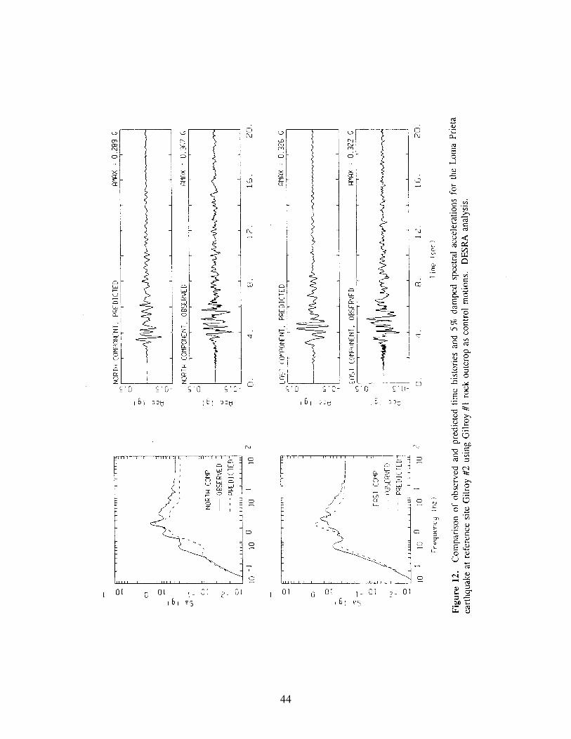
Nonlinear Analysis: DESRA-2C. Results from the DESRA-2C analysis are shown in Figure 12. The

north component shows a general underprediction over most of the frequency range while the east

component shows a much more favorable match. In general however, the tendency is toward overall

underprediction. The time histories appear much more similar to the equivalent-linear RASCAL analysis

than do the response spectra. This indicates that the more robust measure of goodness-of-fit is likely to be

made on spectral ordinates if timing of arrivals is of secondary importance to correct amplitudes.

Nonlinear Analysis: SUMDES. Figure 13 shows the results from the code SUMDES. Although the

north component shows some underprediction, the comparison to the empirical spectra is quite good. The

computed time histories show comparable frequency content and durations to recorded motions as well as

similar coda wave levels. The increase in coda levels over the RASCAL and DESRA-2C analyses

indicate that the effects of the dipping structure are actually quite minimal since the predicted coda

amplitudes now match the observed. Perhaps overdamping in the RASCAL and DESRA-2C analyses

was the cause of reduced coda relative to the recorded motions.

Nonlinear Analysis: TESS. The results from the TESS analysis are shown in Figure 14 and are very

similar to the SUMDES analysis. There is a slight underprediction of the north component with a very

good match to the east component. The overall frequency content, durations, and coda levels compare

very favorably with the recorded motions.

Summary of Gilroy #2 Analyses. As a final comparison, log average response spectra of the horizontal

components for both recorded and computed motions are shown in Figure 15. DESRA shows a general

underprediction over much of the frequency range while RASCAL provides a good overall match with an

overprediction of the resonance near 3 Hz. This is not unexpected in equivalent-linear analyses since the

13

velocities are constant at the strain compatible values, while in nonlinear analyses they vary with time.

As a result, resonance phenomena are less well pronounced in nonlinear analyses at high strain levels and

may, in fact, depend upon the character (duration) of the control motion.

In an overall sense the comparisons are considered quite favorable with RASCAL, SUMDES, and TESS

showing generally better agreement to recorded motions. The vertically-propagating shear-wave model

appears to result in very favorable comparisons to recorded motions. Both equivalent-linear and

nonlinear analyses show very similar results and an increase in damping, from 3% to about 7%, with

increasing levels of motion is required to model both weak and strong motions.

Treasure Island

As with reference site Gilroy #2, ground motions from the 1989 M 6.9 Loma Prieta earthquake were

analyzed. Recordings at Yerba Buena Island were used as adjacent (. 2 km) rock outcrop control

motions. Table 4 lists the control motion peak accelerations and source-to-site distance.

Linear Analyses. Figure 16 shows the small-strain transfer functions (Treasure Island/Yerba Buena

Island) computed from recordings of 7 aftershocks (Jarpe et al., 1989). Also shown is the computed

transfer function using the base-case shear-wave velocity profile (Figure 3). The empirical transfer

function exceeds the computed by a factor of nearly three for frequencies up to about 7 Hz. The locations

of the resonances are predicted quite well by one-dimensional linear analysis out to the same frequency.

Because the shapes in the empirical and theoretical transfer functions show good agreement out to about 7

Hz, it is difficult for the effects of basement topography to be the cause of the largely constant offset over

this frequency range.

The sharp drop in the empirical ratio near 7 Hz is due largely to a sharp drop in the Treasure Island

Fourier amplitude spectra. This may be a result of unmodeled shallow soil structure since the boreholes

were not placed at the exact location of the recording instrument. The only remaining sources of the

discrepancy are the control motions, perhaps being deficient for frequencies up to about 7 Hz or high in

energy beyond 7 Hz relative to the basement of Treasure Island, and the impedance contrast from soil to

rock at Treasure Island. The control motions could simply be inappropriate due to topographic effects at

Yerba Buena Island although this is not obvious from visual examination of the Fourier amplitude

14

spectra. The basement shear-wave velocity was taken as 3500 ft/sec (Figure 3) based upon suspension

logging results. If a large velocity gradient exists below the existing hole such that shear-wave velocities

of about 10,000 ft/sec were reached within 100-200 ft, results of analyses indicate that the computed ratio

would move up to the level of the empirical. It should also be pointed out that this process assumes that

the same gradient does not exist under the recording site at Yerba Buena Island.

This large relatively constant difference of a factor near three in the empirical and theoretical transfer

functions is an important issue. A number of researchers (Idriss, 1990; Dickenson et al., 1991; Hryciw et

al., 1991) have used this soil/rock station pair with similar profiles in site response studies. The results

have been used to adjust model parameters and make inferences regarding the ability of different

procedures to model recorded motions as well as predict liquefaction. Until this issue is resolved by

recording small earthquakes at the surface, at some depth in the basement at the Treasure Island site, and

at the Yerba Buena site, as well as extending the deep hole further into basement rock and measuring

velocities, uncertainty will remain in interpreting results in site response analyses using the strong motion

recordings from these sites.

The linear analysis results for the Loma Prieta earthquake are shown in Figure 17. The computed spectra

show a general underprediction up to about 2-3 Hz and match the recorded motions reasonably well

beyond. Of interest, the predicted spectral peaks occur at higher frequencies than in the recorded strong

ground motions but are matched very well in the weak motion transfer functions.

The computed time histories reflect the low-frequency deficiency shown in the spectra, particularly the

east component, and match the observed peak accelerations quite well. It is important to point out, in

examining the recorded and computed time histories, that no adjustment has been made for absolute time.

For example, Figure 17 suggests that the predominant motion in the computed motions arrives before that

of the recordings. Neither the difference in trigger times of the recorders at Treasure Island and at Yerba

Buena Island nor the differential travel times has been accounted for.

The broad-band nature of the underprediction, seen now down to 0.1 Hz, likely reflects the same

phenomenon exhibited by the small-strain Fourier spectral ratios and further suggests a large scale feature

such as a larger impedance contrast or a steep velocity gradient at the base of the Treasure Island profile.

15

Equivalent-Linear Analysis: RASCAL. Figure 18 shows the results of the equivalent-linear analysis. As

expected, very little difference from the linear analysis is seen in the computed spectra below about 1 Hz.

The fundamental resonance is at about 0.7 Hz and is clearly seen on both components. The higher

resonances are shifted to lower frequencies in the equivalent-linear analysis and more closely match the

empirical spectra, particularly on the larger of the two components (east). The underprediction now

extends over most of the frequency range due to the increased damping in the profile associated with the

equivalent-linear analysis. This is reflected in the time histories as well, showing less high-frequency

energy and reduced peaks. Increasing the control motion uniformly would result in a direct (one-to-one)

enhancement of low frequencies but, due to resulting increase in strain levels and accompanying higher

damping, show less of an effect at high frequencies. Increasing the impedance contrast at the soil/rock

interface would have such an effect.

Other workers have obtained different results at this site using similar methodologies with different

material properties, modified control motions, and by varying sensitive parameters in the computer codes.

This points out that better or worse comparisons may be obtained for earthquakes which have occurred.

The intent of the present analyses was to perform, to the extent possible, a forward prediction at each site

using measured material properties and implementing the analysis procedures in a consistent manner.

The results then provide a more rational basis for evaluating how well the prediction methodologies

perform.

Nonlinear Analysis: DESRA-2C. Figure 19 shows the results from the DESRA-2C analysis. The

computed response spectra show an overall underprediction to the observations, similar to the RASCAL

results. The motions computed with DESRA-2C show more low-frequency energy on the east component

and less high-frequency energy on the north component. These trends are reflected in the computed time

histories as well. In general however, the DESRA-2C and equivalent-linear results are comparable.

Nonlinear Analysis: SUMDES. Results from the SUMDES analysis are shown in Figure 20. For the

north component, the SUMDES motions show slightly higher levels while the east- component motions

are significantly higher. The spectrum computed for the east component matches the observed very well

up to about 1.3 Hz and beyond 10 Hz, missing the resonances at 3 and at 7 Hz. The time history for the

16

east component also matches the observed quite well with only a 7% underprediction in peak acceleration.

As with the previous analyses, however, the amplitude, duration, and character predicted for the north

component does not match the observed very well.

Nonlinear Analysis: TESS. The results for the TESS analysis are shown in Figure 21 and indicate

similar features to the other analyses. A general broad-band underprediction of motions is shown for both

components and a poor characterization of the waveform for the north component are seen.

Summary of Treasure Island Analyses. A comparison of the average spectra is shown in Figure 22. In

the figures, the overall broad-band nature of the underprediction is quite apparent. All four analyses

produce comparable levels of computed motions when the components are averaged. These results are in

accord with the Gilroy #2 analyses and suggest that the equivalent-linear and nonlinear analyses produce

very similar strong ground motion predictions for these levels of motion and soil conditions. For the

Treasure Island site, results from the equivalent-linear and nonlinear analyses are comparable to the linear

analysis, indicating that nonlinear soil effects, in terms of surface ground motions, were not significant

during the Loma Prieta earthquake. This is in accord with the observations of Silva and Stark (1992).

The similar pattern in broad-band underprediction suggests that the Yerba Buena control motion may be

inappropriate as input to the Treasure Island profile, perhaps due to topographic effects. Alternatively, or

in conjunction, a strong velocity gradient may exist in the bedrock beneath the Treasure Island site that is

not present at the Yerba Buena site. Until this issue is resolved, results of analyses with these recordings

will have uncertainties regarding inferences on both site response analysis procedures and nonlinear soil

models.

Lotung

At the Lotung reference site, data from a vertical array of three component accelerometers were used.

Sensor packages are located at the surface and depths of 20 ft (6 m), 36 ft (11m), 56 ft (17m), and 154 ft

(47m) (Anderson and Tang, 1989). Data from three earthquakes were analyzed, two of which represent

strong motion with surface peak acceleration values near 10%g (Table 4, LSST events 7 and 16). A third

earthquake (LSST event 10), with an average surface peak acceleration value of about 4%g was used for a

small-strain analysis to assess the appropriateness of the base-case or low strain profile (velocity and

17

damping) and the vertically- propagating shear-wave assumption. Events 7 and 10 have recordings at all

5 levels and event 16 recordings are available from the top 4 levels (surface, 20 ft, 36 ft, and 56 ft).

Interestingly, even at these low levels of motion, the profile appears to have gone nonlinear, which is

consistent with the results of Silva et al. (1990).

For the strong motion analyses, LSST events 7 and 16 were used as control motions (Table 4). Analyses

consist of propagating the motions recorded at the deepest sensor package to the surface. For LSST event

7 the recordings at 154 ft were used while for LSST event 16, the deepest recordings were at the 56 ft

level. Results are presented for analyses from the deepest recording levels to the surface. (For results of

analyses from the deepest levels to subsurface levels see EPRI, 1993).

Linear Analysis. The small-strain transfer function computed for LSST event 10 using a linear analysis is

shown in Figures 23-25 for surface to 154 ft, 36 to 154 ft, and 56 to 154 ft respectively. The control

motion was taken from the recordings at 154 ft (Table 4). Although the frequencies of the peaks are

matched reasonably well for all the ratios out to about 10 Hz, indicating an appropriate shear-wave

velocity profile and wave-propagation model, the predicted amplitudes are high, particularly for the

higher order resonances. The small-strain damping was fixed at 1% for the profile based on the damping

curves (Figure 6, 10-4% shear strain) and the computed ratios indicate that this value may be too low.

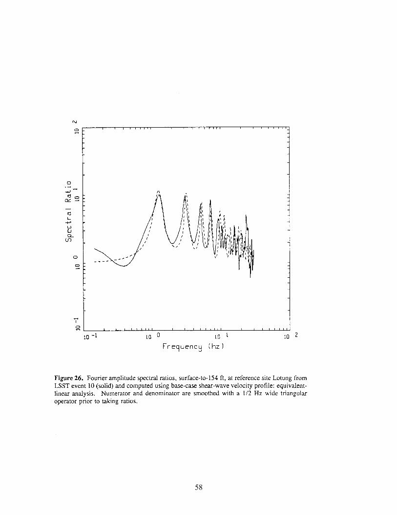
The small-strain analysis was repeated using the equivalent-linear approach and the resulting transfer

functions are shown in Figures 26-28. The equivalent-linear transfer functions show a significant

reduction in amplitude and a slight shift in predominant frequencies. The overall fit is measurably

improved. The average damping throughout the profile increased from 1.0 to 1.7% which suggests that at

soft sites, nonlinear soil response can have effects even at surface acceleration levels of 3-4%g.

To explore the effects of increased levels of recorded motions, an analysis of the frequencies and

amplitudes of the fundamental resonance peaks was done for the three earthquakes studied (LSST events

7, 10, and 16). The surface-to-depth ratios (20, 36, 56 and 154 ft) were analyzed and the results are

shown in Table 5. The trend in reduced frequencies and amplitudes of the fundamental resonance with

increasing levels of surface motion (average PGA = 0.035g, 0.115g, and 0.183g) is clear. There is more

than a factor of two shift in frequency and amplitude at all levels except surface/154 ft. For this ratio, the

18

deeper soils have higher velocities, develop lower strain levels, and the frequency shift and amplitude

reduction are correspondingly less. These results present a compelling case for in-situ nonlinear soil

response and suggest that these effects could extend to large source-to-site distances from large to

moderate earthquakes for soft sites.

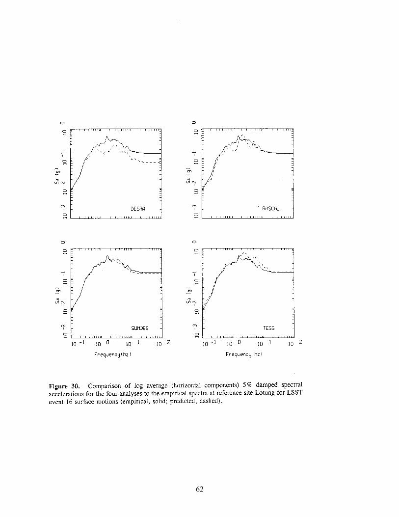
Equivalent-Linear Analysis: RASCAL. To reduce the number of figures, only the average response

spectra (two components) resulting from the site response analyses are presented in Figures 29 and 30 for

events 7 and 16. The complete set of individual spectra and time histories are contained in EPRI (1993).

Results of the equivalent-linear analyses (RASCAL) for LSST events 7 and 16 indicate that the predicted

spectra agree in overall shape and level with the empirical for both earthquakes. The resonances tend to

be overpredicted in most cases, particularly for event 7, but the agreement between the predicted and

empirical spectrums is generally quite good. The vertically propagating shear-wave model and laboratory

derived material strain dependencies appear to provide an accurate representation of the response of this

profile throughout the upper 154 ft.

Nonlinear Analysis: DESRA-2C. For event 7, the motions computed at the surface using DESRA-2C

(Figure 29) are very close to the empirical, except for the low response for frequencies above 3-4 Hz. For

event 16 (Figure 30), there is a general underprediction at the surface above about 0.4 Hz.

In general, the results of DESRA-2C are not as good as those using the equivalent-linear analysis

technique. This is opposite to the results of Chang et al. (1990), although the differences between the

equivalent-linear and nonlinear results were much less than is shown here. Chang et al. used a modified

version of the DESRA code by incorporating a Martin-Davidenkov soil model to analyze event 7. The

study also used a different soil profile as well as different modulus reduction and damping curves.

Additionally, in the Chang et al. study the control motion was at 56 ft, rather than at the 154 ft level used

here. As a result, the propagation paths are much shorter. The use of deeper motions reduces the possible

contamination of the control motion by surface-generated scattered wavefields (Silva et al., 1988) and is a

more stringent test of the 1-dimensional wave propagation methodology. As a result of these differences,

it is difficult to compare the results of the two studies in a meaningful way, and it would be of interest to

repeat the present study using the Martin-Davidenkov soil model.

19

Nonlinear Analysis: SUMDES. For LSST event 7, the results using SUMDES are similar to DESRA-

2C at the surface but show less of an underprediction above around 3 Hz. The results for event 16 (Figure

30), on the other hand, show excellent agreement with the recorded motions. The match in the spectral

ordinates is quite good particularly below about 3 Hz.

Nonlinear Analysis: TESS. For LSST event 7, the results for TESS match the response spectra very

well and are comparable to the SUMDES results. The overall shapes of the response spectra agree very

well with the empirical and even matches in detail at several frequencies from about 1 to 10 Hz. The

corresponding results for event 16 are shown in Figure 30. For this earthquake, the match is also quite

good. A tendency exists for a slight broad-band overprediction of the average spectrum, particularly from

about 2 to 15 Hz.

Summary of Lotung Analyses. A significant aspect of the Lotung analyses is a suggestion of nonlinear

soil response at very low levels of surface peak acceleration (4%g), as well as a clear demonstration of

consistent frequency shifts and decreases in resonance peaks with increasing levels of motion. These

results, when considered with the linear analyses of events 7 and 16, show that a large increase in shear-

wave damping is taking place in going from surface accelerations of 3%g to levels of 12% to 18%g.

Results of the equivalent-linear and nonlinear analyses for the same earthquakes, summarized in the

average response spectra shown in Figures 29 and 30, indicate that the laboratory-derived dynamic

material properties reflect the in-situ strain dependencies very well. The average spectra also show, for

both earthquakes, very similar results for the equivalent-linear and nonlinear analyses. The individual

component analyses showed that some approaches performed better than others for certain components,

depths, and earthquakes but, on average, each approach produces comparably good results.

The vertically-propagating shear-wave model represents an accurate representation of the predominant

motion at this site over the frequency range of 0.1 to over 30 Hz for the three earthquakes studied. In

addition, the equivalent-linear results are generally comparable to those of the nonlinear analyses with a

tendency to overpredict the resonances, particularly the fundamental. All of these results are consistent

with those of the other sites: Gilroy #2 and Treasure Island.

20

Conclusions

The major issues involved in the prediction of the effects of site response to strong ground motions

include a suitable wave propagation model, the in-situ strain dependencies of dynamic material properties,

and how the effects of material nonlinearities are treated computationally. In the work presented here, the

intent was to treat all three aspects by comparing observed strong ground motions to predicted motions at

three carefully characterized reference sites. Reasonably comprehensive geotechnical models based in

part on laboratory testing were developed for Gilroy #2, Treasure Island, and the Lotung, Taiwan LSST

site. The sites possess all of the features which were thought necessary to provide a good validation:

recordings of both high- and low-strain ground motions, a dipping interface at least at one site (Gilroy

#2), a wide range in material properties from sands and gravels to soft silts and stiff clays, deep (70 ft) and

shallow (surface) water tables, and a wide range in stiffness from deep and stiff at Gilroy #2 to shallow

and very soft at Lotung.

All analysis procedures compared used the vertically-propagating shear-wave model and included

equivalent-linear, implemented through the RVT based RASCAL code, and three nonlinear

methodologies: DESRA, SUMDES, and TESS. Results using small-strain data and linear analyses show

low-strain laboratory damping measurements to be consistent with transfer functions calculated using

recordings from small earthquakes. For strong ground motions, and even weak motions at the Lotung

LSST site, nonlinear soil response was observed and modeled very well by both the equivalent-linear and

nonlinear techniques. Both computational approaches to model the effects of soil nonlinearity produced

equally good comparison to recorded ground motions both in response spectra and time histories.

In both the small- and large-strain analyses at the soil/rock site pair (Gilroy #2/Gilroy #1) with a known

dipping interface between the sites, 2- or 3-dimensional effects were shown to be small and not

considered in modeling the site response from either the Loma Prieta earthquake or recordings of

aftershocks. Results from the simple vertically-propagating shear-wave model provided a very favorable

comparison to observed motions from 0.1 Hz to over 30 Hz for the mainshock and from about 2 Hz to 20

Hz for the aftershocks (the bandwidth of useable data).

At reference site Treasure Island, a large discrepancy exists between the computed transfer function using

the base-case shear-wave velocity profile and the average empirical transfer function from aftershocks

21

recorded at Treasure Island and Yerba Buena Island. The empirical transfer function exceeds the

analytical by a factor of about 2-3 for frequencies up to nearly 10 Hz. Nonlinear soil response does not

appear to be the cause of this discrepancy as the computed motions for the Loma Prieta earthquake using

the Yerba Buena recordings as control motions show a broad-band and general underprediction of the

recorded motions. It is suggested that either or both a topographic effect at Yerba Buena Island or a large

velocity gradient beneath the level of measured velocities at Treasure Island may be responsible. Until

this issue is resolved, uncertainties will remain regarding analyses done with this pair of strong motion

recordings.

Results of the analyses at Lotung suggest that nonlinear effects can be present in soft soils for surface

peak acceleration values as low as 4%g (cyclic shear strains exceeding 10-2%). Additionally, a clear and

dramatic shift in resonant peaks to lower frequencies and reduction in amplitude is shown for increasing

levels of motion. The generally good match to recorded motions provided by the nonlinear and

equivalent-linear analyses show that the in-situ material strain dependencies are accurately modeled by

careful laboratory analyses.

The general conclusion resulting from these analyses is that conventional one-dimensional site response

analyses incorporating nonlinear soil behavior based upon careful laboratory testing and with reasonably

accurate soil profiles can accurately predict the effects of soils on strong ground motions.

22

REFERENCES

Aki, K. (1988). Local site effects on ground motion. Earthquake engineering and soil Dynamics II-Recent Advances in Ground-Motion Evaluation, Proc. Am. Soc. Civil. Engin. Specialty Conf., Park City, Utah, Pub. 20:103-155.

Andersen, D.G. and Y.K. Tang (1989). Summary of soil characterization program for the Lotung Large-

Scale Seismic Experiment. Proceedings: EPRI/NRC/TPC Workshop on Seismic Soil-Structure Interaction Analysis Techniques using Data from Lotung, Taiwan. Palo Alto, Calif.: Electric Power Research Institute, NP-6154, 1:4-1 to 4-20.

Benites, R., W.J. Silva and B. Tucker (1985). Measurements of ground response to weak motion in La

Molina Valley, Lima, Peru. Correlation with strong ground motion. Earthquake Notes, Eastern Section, Bull. Seism. Soc. of Am., 55(1).

Berrill, J.B. (1977). Site effects during the San Fernando, California, earthquake. Proceedings of the

Sixth World Conf. on Earthquake Engin., India, 432-438. Borcherdt, R.D. and J.F. Gibbs (1976). Effects of local geologic conditions in the San Francisco Bay

region on ground motions and the intensities of the 1906 earthquake. Bull. Seism. Soc. Am., 66:467-500.

Borcherdt, R.D. and G. Glassmoyer (1992). On the characteristics of local geology and their influence

on ground motions generated by the Loma Prieta Earthquake in the San Francisco Bay region, California. Bull. Seism. Soc. Am., 82(2):603-641.

Chang, C.-Y., C.M. Mok, M.S. Power, Y.K. Tang, H.T. Tang and J.C. Stepp (1990). Equivalent linear

versus nonlinear ground response analyses at Lotung seismic experiment site. Proceedings of the Fourth U.S. Nat'l Conf. on Earthquake Engin., 1:327-336.

Chin, B.H. and K. Aki (1991). Simultaneous study of the source, path, and site effects on strong ground

motion during the 1989 Loma Prieta earthquake: a preliminary result on pervasive nonlinear site effects. Bull. Seism. Soc. Am., 81(5):1859-1884.

Darragh, R.B. and A.F. Shakal (1991). The site response of two rock and soil station pairs to strong and

weak ground motion. Bull. Seism. Soc. Am., 81(5):1885-1899. Day, S.M. (1979). Three-dimensional finite difference simulation of fault dynamics. Systems, Science

and Software final report sponsored by the National Aeronautics and Space Administration. SSS-R-80-4295.

Dickenson, S.E., R.B. Seed, J. Lysmer and C.M. Mok (1991). Response of soft soils during the 1989

Loma Prieta Earthquake and implications for seismic design criteria. Proceedings, Pacific Conf. on Earthquake Engin., Auckland, New Zealand.

Dimitriu, P.P., Ch. A. Papaioannou, and N.P. Theodulidis (1998). “Euro-seistest strong-motion array near

Thessaloniki, Northern Greece: A study of site effects.” Bull. Seism. Soc. Am.,88(3),862-873.

23

Drnevich, V.P., J.R. Hall Jr. and F.E. Richart Jr. (1966). Large amplitude vibration effects on the shear

modulus of sand. University of Michigan Report to Waterways Experiment Station, Corps of Engineers, U.S. Army, Contract DA-22-079-eng-340.

Duke, C.M. and A.K. Mal (1978). Site and source effects on earthquake ground motion. Univ. of Calif.

Los Angeles Engin., Report No. 7890. Electric Power Research Institute (1993). Guidelines for determining design basis ground motions. Palo

Alto, Calif: Electric Power Research Institute, vol. 1-5, EPRI TR-102293. vol. 1: Methodology and guidelines for estimating earthquake ground motion in eastern North America. vol. 2: Appendices for ground motion estimation. vol. 3: Appendices for field investigations. vol. 4: Appendices for laboratory investigations. vol. 5: Quantification of seismic source effects.

Elgamal, A. W., M . Zeghal and E. Parra (1996). "Liquefaction of Reclaimed Island in Kobe, Japan."

Japan Journal, Geotechnical Engineering, ASCE, 39_49. Faccioli, E.E., V. Santayo and J.L. Leone (1973). Microzonation criteria and seismic response studies for

the city of Managua. Proceedings of Earthquake Engin. Res. Dist. Conf. Managua, Nicaragua, Earthquake of December 23, 1972, 1:271-291.

Field, E.H., K.H Jacob and S.E. Hough (1992). Earthquake site response estimation: a weak-motion case

study. Bull. Seism. Soc. Am., 82(6):2283-2307. Ganev, T., F. Yamazaki, H. Ishizaki, and M. Kitazawa (1998). “Response analysis of the Higashi-Kobe

bridge and surrounding soil in the 1995 Hyogoken-Nanbu.” Earth. Engng. Struct. Dyn., 27, 557-576.

Gutenberg, B. (1957). Effects of ground on earthquake motion. Bull. Seism. Soc. Am., 47:221-250. Hardin, B.O. and V.P. Drnevich (1972). Shear modulus and damping in soils: measurements and

parameters effects. J. Soil Mech. and Found. Div. ASCE, 98(SM6):603-624. Hartzell, S.H. (1992). Site response estimation from earthquake data. Bull. Seism. Soc. Am.,

82(6):2308-2327. Haskell, N.A. (1960). Crustal reflection of plane SH waves. J. Geophys. Res., 65:4147-4150. Hays, W.W., A.M. Rogers and K.W. King (1979). Empirical data about local ground response.

Proceedings of the Second U.S. Nat. Conf. on Earthquake Engin., Earthquake Engin. Res. Inst., 223-232.

24

Hryciw, R.D., K.M. Rollins, M. Homolka, S.E. Shewbridge and M. McHood (1991). Soil amplification at Treasure Island during the Loma Prieta Earthquake. Proceedings of the Second Int'l Conf. on Recent Advances in Geotech. Earthquake Engin. and Soil Dynamics, St. Louis, Paper No. LP20.

Hutchings, L.J. and F. Wu (1990). Empirical Green's functions from small earthquakes: a waveform

study of locally recorded aftershocks of the 1971 San Fernando earthquake. J. Geophys. Res. 95:1187-1214.

Idriss, I.M. (1990). Response of soft soil sites during earthquakes. Presented at a Memorial Symposium

to Honor Prof. Harry Seed, Univ. of Calif. at Berkeley. Idriss, I.M. and H.B. Seed (1968). Seismic response of horizontal soil layers. Proceedings of the Amer.

Soc. Civil Engin., J. Soil Mech. and Found. Div., ASCE, 94:1003-1031. Iwan, W.D. (1967). On a class of models for the yielding behavior of continuous and composite systems.

J. Appl. Mech., 34:612-617. Jarpe, S.P., L.J. Hutchings, T.F. Hauk and A.F. Shakal (1989). Selected strong- and weak-motion data

from the Loma Prieta sequence. Seism. Res. Lett., 60:167-176. Joyner, W.B. and A.T.F. Chen (1975). Calculation of nonlinear ground response in earthquakes. Bull.

Seism. Soc. Am., 65:1315-1336. Joyner, W.B., R.E. Warrick and A.A. Oliver III (1976). Analysis of seismograms from a downhole array

in sediments near San Francisco Bay. Bull. Seism. Soc. Am., 66:937-958. Lee, M.K.W. and W.D.L. Finn (1991). DESRA-2C: Dynamic effective stress response analysis of soil

deposits with energy transmitting boundary including assessment of liquefaction potential. The University of British Columbia, Faculty of Applied Science.

Li, X.S., Z.L. Wang and C.K. Shen (1992). SUMDES: A nonlinear procedure for response analysis of

horizontally-layered sites subjected to multi-directional earthquake loading. Dept. of Civil Engin. Univ. of Calif., Davis.

Martin, P.P. (1975). Non-linear methods for dynamic analysis of ground response. Ph.D. Thesis, Univ. of

Calif. at Berkeley. McGuire, R.K., G.R. Toro and W.J. Silva (1988). Engineering model of earthquake ground motion for

Eastern North America. Palo Alto, Calif.: Electric Power Research Institute, RP 2556-16. Moriwaki, Y., R. Pyke, M. Bastick and T. Udaka (1981). Specification of input motions for seismic

analyses of soil-structure systems within a nonlinear analyses framework. Palo Alto, Calif.: Electric Power Research Institute, NP-2097.

Murphy, J.R., A.H. Davis and N.L. Weaver (1971). Amplification of seismic body waves by low-

velocity surface layers. Bull. Seism. Soc. Am., 61:109-145.

25

Power, M.S., J.A. Egan, S. Shewbridge, J. Debecker and J.R. Faris (1993). Analysis of liquefaction-

induced distress at Treasure Island. NEHRP report on the Loma Prieta earthquake, in press. Prevost, J.H. (1989). DYNA1D: A computer program for nonlinear seismic site response analysis,

technical documentation. Nat'l Center for Earthquake Engin, Res., Technical report NCEER-89-0025.

Pyke, R.M. (1979). Nonlinear models for irregular cyclic loadings, J. Geotech. Engin. Div., ASCE,

105(GT6):715-726. Pyke, R.M. (1992). TESS: A computer program for nonlinear ground response analyses. TAGA Engin.

Systems & Software, Lafayette, Calif. Reid, H.F. (1910). The California earthquake of April 18, 1906. The Mechanics of the Earthquake.

Carnegie Inst. of Washington, Publ. 87, 21. Richart, F.E. (1975). Some effects of dynamic soil properties on soil-structure interaction. J. Geotech.

Engin. Div., ASCE, 101(GT12):1197-1240. Rogers, A.M., R.D. Borcherdt, P.A. Covington and D.M. Perkins (1984). A comparative ground response

study near Los Angeles using recordings of Nevada nuclear tests and the 1971 San Fernando earthquake. Bull. Seism. Soc. Am., 74: 1925-1949.

Satoh, T., T. Sato, and H. Kawase (1995). “Nonlinear behavior of soil sediments identified by using

borehole records observed at the Ashigar Valley, Japan.” Bull. Seism. Soc. Am., 85(6), 1821-1834. Schnabel, P.B., J. Lysmer and H.B. Seed (1972). SHAKE: a computer program for earthquake response

analysis of horizontally layered sites. Earthquake Engin. Res. Center, Univ. of Calif. at Berkeley, UBC/EERC 72-12.

Seed, H.B. and I.M. Idriss (1969). The influence of soil conditions on ground motions during

earthquakes. J. Soil Mech. Found. Engin. Div., ASCE, 94:93-137. Seed, H. B. and I.M. Idriss (1970). Soil moduli and damping factors for dynamic response analyses.

Earthquake Engin. Res. Center, Univ. of Calif. at Berkeley, UCB/EERC-70/10. Seed, H.B., R.T. Wong, I.M. Idriss and K. Tokimatsu (1984). Moduli and damping factors for dynamic

analyses of cohesionless soils. UCB/EERC-84. Silva, W.J. (1976).”Body waves in a layered anelastic soiled.” Bull. Seis. Soc. Am., 66(5):1539- 1554. Silva, W.J. (1991). Global characteristics and site geometry. Chapter 6 in Proceedings: NSF/EPRI

Workshop on Dynamic Soil Properties and Site Characterization. Palo Alto, Calif.: Electric Power Research Institute, NP-7337.

26

Silva, W.J. and C.L. Stark (1991). Near-field and in-structure monitorings of the aftershocks of the 1989 Loma Prieta earthquake. Palo Alto, Calif.: Electric Power Research Institute, Draft Final Report RP 3181-03.

Silva, W.J. and C.L. Stark (1992). Source, path, and site ground motion model for the 1989 M 6.9 Loma

Prieta earthquake. CDMG final report. Silva, W.J., C.L. Stark, S.J. Chiou, R. Green, J.C. Stepp, J. Schneider and D. Anderson (1990). Non-

linear soil models based upon observations of strong ground motions. Seism. Res. Lett., 61(1):13. Silva, W.J., T. Turcotte and Y. Moriwaki (1988). Soil response to earthquake ground motion. Palo Alto,

Calif: Electric Power Research Institute, RP-2556-07. Streeter, V.L., E.B. Wylie and F.E. Richart Jr. (1974). Soil motion computations by characteristics

method. J. Geotech. Engin. Div., ASCE, 100(GT3):247-263. Su, F., K. Aki, T. Teng, Y. Zeng, S. Koyanagi and K. Mayeda (1992). The relation between site

amplification factor and surficial geology in central California. Bull. Seism. Soc. Am., 82(2):580-602.

Taylor, P.W. and T.J. Larkin (1978). Seismic site response of nonlinear soil media. J. Geotech. Engin.

Div., ASCE, 104(GT3). Tucker, B.E. and J.L. King (1984). Dependence of sediment-filled valley response on the input amplitude

and the valley properties. Bull. Seism. Soc. Am., (74):153-165. Valera, J.E., E. Berger, H.-S. Kim, J.E. Reaugh, R.D. Golden and R. Hofmann (1978). Study of nonlinear

effects on one-dimensional earthquake response. Palo Alto, Calif.: Electric Power Research Institute, NP-865.

Wiggins, J.H. (1964). Effects of site conditions on earthquake intensity. J. Structural Div., ASCE, 90(2),

Part I. Wood, H.O. (1908). Distribution of apparent intensity in San Francisco, in the California earthquake of

April 18, 1906. Report of the State Earthquake Investigation Commission, Wash., D.C.: Carnegie Institute, 1:220-245.

27

Table 1

PROPERTIES OF SAMPLES FROM GILROY #2 Sample

No. Sample Depth ft(m)

Soil Description

Liquid Limit %

Plasticity Index %

Water Content

%

Total Unit Weight

pcf (g/cc)

Void Ratio

e

Dry Unit Weight

pcf (g/cc)

Specific Gravity

Gs

Degree of Saturation

% Dark Brown

G1 10 Clayey Silt with 29 7 26.1 117.1 0.78 93 2.70 86 (3.0) Sandy Material (1.88) (1.49) 20 Dark Gray 118.8 91, 96

G2 (6.1) Silty Clay 43 23 30.0 (1.90) 0.84 (1.46, 1.54) 2.70 96 50 Silty Sand 123.4 107

G3 (15.2) with Gravel ----- ----- 15.8 (1.98) 0.58 (1.71) 2.65 76 Light Gray

G4 85 Stiff Clay 47 17 30.8 121.0 0.82 93, 95 2.70 100 (25.9) with Horiz.

Bedding (1.94) (1.49, 1.52)

120 134.1 112, 110 2.65 100 G5 (36.6) Silty Sand ----- ----- 19.8 (2.15) 0.55 (1.79, 1.76)

210 130.1 124 2.65 62 G6 (64.0) Gravelly Sand ----- ----- 14.8 (2.08) 0.52 (1.99)

420 136.4 113 2.65 85 G7 (128.0) Gravelly Clay ----- ----- 28.0 (2.19) 0.58 (1.81)

348 127.7 103 2.70 100 G8 (106.1) Clayey Silt 35 13 23.7 (2.05) 0.60 (1.65)

420 136 120 G9 (128.0) Gravelly Clay ----- ----- 14.0 (2.18) 0.41 (1.92) 2.70 92

28

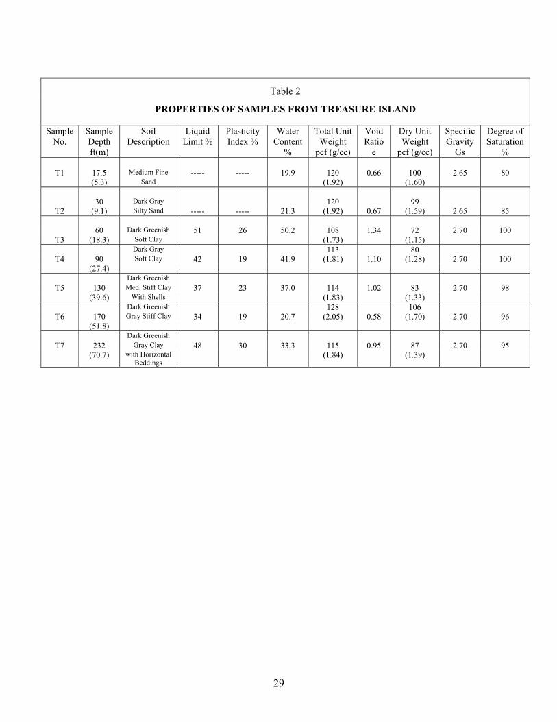
Table 2

PROPERTIES OF SAMPLES FROM TREASURE ISLAND Sample

No. Sample Depth ft(m)

Soil Description

Liquid Limit %

Plasticity Index %

Water Content

%

Total Unit Weight

pcf (g/cc)

Void Ratio

e

Dry Unit Weight

pcf (g/cc)

Specific Gravity

Gs

Degree of Saturation

%

T1 17.5 Medium Fine ----- ----- 19.9 120 0.66 100 2.65 80 (5.3) Sand (1.92) (1.60) 30 Dark Gray 120 99

T2 (9.1) Silty Sand ----- ----- 21.3 (1.92) 0.67 (1.59) 2.65 85 60 Dark Greenish 51 26 50.2 108 1.34 72 2.70 100

T3 (18.3) Soft Clay (1.73) (1.15) Dark Gray 113 80

T4 90 Soft Clay 42 19 41.9 (1.81) 1.10 (1.28) 2.70 100 (27.4) Dark Greenish

T5 130 Med. Stiff Clay 37 23 37.0 114 1.02 83 2.70 98 (39.6) With Shells (1.83) (1.33) Dark Greenish 128 106

T6 170 Gray Stiff Clay 34 19 20.7 (2.05) 0.58 (1.70) 2.70 96 (51.8) Dark Greenish

T7 232 Gray Clay 48 30 33.3 115 0.95 87 2.70 95 (70.7) with Horizontal

Beddings (1.84) (1.39)

29

Table 3

PROPERTIES OF SAMPLES FROM LOTUNG LSST

Sample No.

Sample Depth ft(m)

Soil Description

Liquid Limit %

Plasticity Index %

Water Content

%

Total Unit Weight

pcf (g/cc)

Void Ratio

e

Specific Gravity

Gs

Degree of Saturation

% 18 112

CH1(T1) (5.5) Silt ----- ----- 31.0 (1.79) 0.93 2.65 88 34.5 118

CH2(T5) (10.5) Silt ----- ----- 32.5 (1.89) 0.85 2.65 100 59 Silty Fine 109

CH1(T4) (18.0) Sand ----- ----- 33.3 (1.75) 1.02 2.65 87 93.5 119

CH2(T9) (28.5) Silty Sand ----- ----- 31.2 (1.91) 0.82 2.65 100 113 118

CH1(T8) (34.5) Clayey Silt 32 7 35.3 (1.89) 0.92 2.70 100 133 117

CH2(T11) (40.5) Clayey Silt 33 8 31.1 (1.88) 0.89 2.70 95 146 128

CH1(T10) (44.5) Silt ----- ----- 24.0 (2.05) 0.56 2.65 100

30

Table 4 TEST SITES AND GROUND MOTIONS

PGA (g) Earthquake

M

Site Distance(km) NS EW

1989 Loma Prieta

6.9 Gilroy #1 Gilroy #2

12 14

0.411 0.367

0.473 0.322

Yerba Buena Is. Treasure Is.

77 79

0.029 0.100

0.068 0.159

LSST Event 7 05/20/86 6.5

LSST-DB47 (154 ft depth)(Surface) 64

0.099 0.208

0.081 0.158

LSST Event 16 11/14/86 7.8

LSST-DB17 (56 ft depth) (Surface) 79

0.086 0.170

0.074 0.133

LSST Event 10 07/16/89 4.5

LSST-DB47 (154 ft depth)(Surface) 6

0.020 0.030

0.013 0.040

31

Table 5

FREQUENCY AND AMPLITUDE OF FUNDAMENTAL RESONANCES AT THE LOTUNG LSST SITE

Surface/20 ft

LSST Event Surface AVG

PGA (g) F (Hz) Amplitude 10 0.035 4.83 10.84

16 0.115 3.37 3.78

7 0.183 2.98 2.65

Surface/36 ft 10 0.035 3.37 7.16

16 0.115 2.44 3.38

7 0.183 1.71 2.01

Surface/56 ft 10 0.035 2.44 8.15

16 0.115 1.66 3.68

7 0.183 1.32 2.52

Surface/154 ft 10 0.035 1.22 6.57

16 0.115 -----* -----*

7 0.183 0.78 3.58

*Recording not available

32

33

34

35

36

37

38 38

39

40

41

42

43

44

45

46

47 47

48

49

50

51 51

52 52

53 53

54 54

55 55

56

57 57

58

59

60 60

61 61

62