Properties of NCGPC applied to

nonlinear SISO systems

with a relative degree one or two

EA 4353

with a relative degree one or two

M. DABO, N. LANGLOIS & H. CHAFOUK

GT Commande Prédictive Non Linéaire

ENSAM, Paris

13 janvier 2011

Relative degree of nonlinear SISO systems

Outline

Unconstrained NCGPC

Case of relative degree equal to 1

PropertiesProperties

Example

Case of relative degree equal to 2

Properties

Example

Conclusion and future work

1. Relative degree of NL systems

Definition [Isidori 1995]:

=+=

))(()(

)())(())(()(

txhty

tutxgtxftx&

System considered:

(1)

The relative degree ρ of (1) is said to be well-defined if (1) has the relative degree ρ at all points in an operating set [Chen 2001]

The nonlinear SISO system (1) is said to have a relative degreeρ around x0 if:

(i) for all x in a neighbourhood of x0 and allk < ρ-1,

(ii)

∑= ∂

∂=n

ii

if xfx

x

hxhL

1

)()()(

0)( =xhLL kfg

0)( 01 ≠− xhLL fgρ

where

2. Unconstrained NCGPC

[ ]∫ +=T

dteJ0

2)(ˆ2

1 ττ )(ˆ)(ˆ)(ˆ τωττ +−+=+ ttyte

Criteria to minimize:

where

The control law can be derived under the assumptions [Chen 2003]:

1: zero dynamics exist and are asymptotically stable;

2: all states are accessible for measurements;

3: the system has a well-defined relative degree;

4: the output and the reference are sufficiently many times continuously differentiable with respect totime;

2. Unconstrained NCGPC

∑=

+=+ρ

ρτττ0

)( )(!

)()(ˆk

kk R

ktyty

Taylor’s series expansion:

==

))(()(

))(()(

txhLty

txhty

&

≈+

)(

)(

)(

!1)(ˆ

)( ty

ty

ty

ty

ρ

ρ

ρτττ

M

&L

+=

=

− ))(())(())(()(

))(()(

1)( txutxhLLtxLty

txhLty

fghf

f

ρρρM

&where

In a similar way:

≈+

)(

)(

)(

!1)(

)( t

t

t

t

ρ

ρ

ω

ωω

ρτττω

M

&L

)

2. Unconstrained NCGPC

≈+

)(

)(

)(

!1)(ˆ

)( ty

ty

ty

ty

ρ

ρ

ρτττ

M

&L

Taylor’s series expansion:

)(

)(

ty

ty

&

=Λ

!1)(

ρτττ

ρL

≈+

)(

)(

)(

!1)(

)( t

t

t

t

ρ

ρ

ω

ωω

ρτττω

M

&L

)

=

)(

)()(

)( ty

tytY

ρM

&

=Ω

)(

)(

)(

)(

)( t

t

t

t

ρω

ωω

M

&

2. Unconstrained NCGPC

From

Criteria to minimize:

)()()( ttYtE Ω−= )()()(ˆ tEte ττ Λ=+

[ ]∫ +=T

dteJ0

2)(ˆ2

1 ττ )()()()(2

1

0

tEdtEJT

tt

ΛΛ= ∫ τττ

02 2

0

where Π(T, ρ) is of dimensions (ρ+ 1)×( ρ+ 1)

Let the prediction matrix ∫ ΛΛ=ΠT

t dT0

)()(),( τττρ

0)(),()(

)( =Π

∂∂

tETtu

tEt

ρ

Criteria minimization:

2. Unconstrained NCGPC

Criteria minimization:

−

−−

=

)()(

)()(

)()(

)()( tty

tty

tty

E

ρρ ω

ωω

M

&&

+

−

−−

=−

×

hLuLhL

hL

h

E

fgf

f

11

)(

0ρ

ρ

ρρ ω

ωω

M

&

))(())(( 1 txhLLtxD −= ρLet

[ ]))((0)(

)( 11 txhLL

tu

tEfg

t−

×=

∂∂ ρ

ρ

))(())(( 1 txhLLtxD fg−= ρLet

[ ] 0),(0)(

1 =

+−

−Π×

DuhL

h

TD

fρρ

ρ

ω

ωρ M0)(),(

)(

)( =Π

∂∂

tETtu

tEt

ρ

0)(

=

+−

−Π

DuhL

h

D

f

sρρ ω

ωM where Πs (dimensions 1× (ρ + 1)) is the last row of Π(T,ρ)

2. Unconstrained NCGPC

D cannot vanish for all x ∈ X : see (ii)The relative degree is supposed well-defined

Criteria minimization:

0)(

=

+−

−Π

DuhL

h

D

f

sρρ ω

ωM

−

−Π=

Π ×

hL

h

Duf

ssρρ

ρ

ω

ω

)(

10M

where Πss(dimensions 1×1) is the last element of vector Πs

−

−Π=Π

hL

h

Du

f

sssρρω

ω

)(

M

2. Unconstrained NCGPC

++ 12!12! ρρρρ

−

−ΠΠ= −−

hL

h

Du

f

sssρρω

ω

)(

11M

Resulting control law [Dabo 2009]:

−

−Π=Π

hL

h

Du

f

sssρρω

ω

)(

M

Let −

+++

++= − 1

)1()!(

12!

1

12!),(

1KK

llTTTK

ρρρ

ρρρρ ρρ

[ ]))((

)())((

))((1

0

)(

txhLL

ttxhLK

txufg

l

llfl

−=∑ −−

= ρ

ρ

ρ ω

Let sssTK ΠΠ= −1),( ρ

1)1(

12

!

!−++

+= ρρ ρρρ

TllK lwhere is the (l+1)th element of K(T, ρ)

2. Unconstrained NCGPC

−

−−

=

=

−− )1()1(

2

1

ρρρ ω

ωω

y

y

y

z

z

z

ZM

&&

M

Change of coordinates:

+−=

==

− hLuLhLz

zz

zz

fgf1)(

32

21

ρρρρ ω&

M

&

&

==

CZO

AZZ&

−−−−

=

− )1(210

1000

0000

0100

0010

ρρρρρ KKKK

A

L

L

MOMMM

L

L

L

1)1(

12

!

!−++

+= ρρ ρρρ

TllK l

with

Resulting linear (and controllable) system:

where

0)( 10 =+++= ρρρρ λλλ LKKPCharacteristic polynomial:

3. Case of relative degree ρ = 1

λλ += 101 )( KP

Characteristic polynomial:

p

GpH

θ+=

1)( 1

1

Corresponding system:

1

Parameter identification:

The application of NCGPC to SISO nonlinear system of dimension 1 equal to its relativedegree, leads, in the right space of coordinates, to a linear 1st-order system with transferfunction H1 defined by a time constant θ and a static gain G1 equal to the referencesignal ω1(t).

Theorem 1:

32T=θ

=

=

1

1

11

10

K

Kθ 1

12!10 +

+=ρρρ

ρTKand

3. Case of relative degree ρ = 1: some properties

Closed-loop system stability:

Predictionhorizon time

Time constant 32T=θ

T

Characteristic parameters/times:

Settling time at 5%

Cut-off frequency

Tc 23=ω

Tt 2%5 ≈

Pole T23−=λ

3. Case of relative degree ρ = 1: example

=+=

)()(

)()(3)( 2

txty

tutxtx&

System considered:

System analysis:

system dimension = 1

Prediction timeT (s)

K1= [K10 K11]

1 [1.5 1]

2 [0.75 1]

3 [0.5 1]

Parameter values vs. T:

system dimension = 1

relative degree = 1

No zero dynamics

3 [0.5 1]

4 [0.375 1]

5 [0.3 1]

Control law:

[ ]))((

)())(()1,(

))((0

1

0

)(1

txhLL

ttxhLTK

txufg

l

llfl∑

=

−−=

ω

Desired output:

step

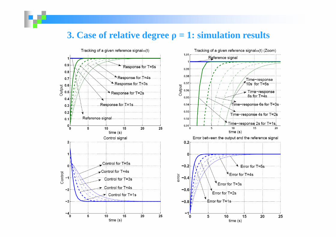
3. Case of relative degree ρ = 1: simulation results

4. Case of relative degree ρ = 2

221202 )( λλλ ++= KKP

Characteristic polynomial:

222

22

)(nn pp

GpH

ωξω ++=

Corresponding system:

1

12!

++=

ρρρω ρT

n = 220K nω

Parameters identification:

T83.1≈ω =+ ωρρ 12! 2

1+=

ρω ρT

n

( )( )( )22 2

121!

2

1),(

+++= − ρ

ρρρρξ ρTT

===

1

2

22

21

20

K

K

K

n

n

ξωω

Theorem 2:

The application of NCGPC to SISO nonlinear system of dimension 2 equal to its relative

degree, leads, in the right space of coordinates, to a 2nd-order linear transfer function with

a constant damping ratio and a natural frequency .685.0≈ξ Tn 83.1≈ω

Tn 83.1≈ω

685.0≈ξ

=++

=++

− n

n

T

T

ξωρρρ

ωρρρ

ρ

ρ

22

12!1

12!

1

2

4. Case of relative degree ρ = 2: some properties

Characteristic parameters/times:

Predictionhorizon time

Rise time

Time-to-peak

Ttr 47.1≈

T

Ttp 34.2≈

Closed-loop system stability:

Time-to-peak

Resonant frequency Tr 46.0≈ω

Tt 39.2%5 ≈Settling time at 5%

Poles )33.125.1(12,1 j

T±−=λ

Ttp 34.2≈

Percent overshoot 21.5≈PO

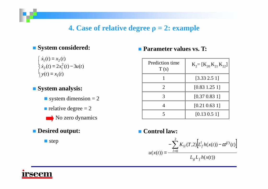
4. Case of relative degree ρ = 2: example

=−=

=

)()(

)(3)(2)(

)()(

1

212

21

txty

tutxtx

txtx

&

&

System considered:

Prediction timeT (s)

K2= [K20 K21 K22]

1 [3.33 2.5 1]

2 [0.83 1.25 1]

3 [0.37 0.831]

Parameter values vs. T:

System analysis:3 [0.37 0.831]

4 [0.21 0.63 1]

5 [0.13 0.5 1]

Control law:

[ ]))((

)())(()2,(

))((

2

0

)(1

txhLL

ttxhLTK

txufg

l

llfl∑

=

−−=

ω

system dimension = 2

relative degree = 2

No zero dynamics

Desired output:

step

4. Case of relative degree ρ = 2: simulation results

Conclusion and future work

Properties of NCGPC when applied to NL SISO systems with:

Relative degree equal to 1: stability, speed & accuracy (step)

Relative degree equal to 2: stability, speed & accuracy (step)

Criteria based on error and control signal

Robustness

Nonlinear Discrete-time GPC

Constraints on actuators

Fault tolerant NDGPC

Thank you for Thank you for your attention!your attention!your attention!your attention!

Appendix 1. Case of 1st-order system: some properties

Appendix 2. Case of 2nd-order system: some properties