PropCode2 Notes

Charles Rino

September 2010

1 Introduction

PropCode2 is a MATLAB implementation of the algorithm described in Chap-ter 3 of The Theory of Scintillation with Applications in Remote Sensing byCharles L. Rino, JohnWiley & Sons IEEE Press, 2010. The algorithm simulateselectromagnetic (EM) wave propagation in a fully three-dimensional medium.Although PropCode2 is a direct extension of PropCode1, it is con�gured to ex-plore the statistical theory of scintillation. The statistical theory con�nes thestructure con�gurations to realizations of statistically homogeneous processes,as described in book Chapter 3. Homogeneous processes admit position invari-ant moments and a spectral density function (SDF). Turbulence is characterizedby a power-law SDF. The directory

nAtmosphereScintillation

contains MATLAB utilities to support the turbulence model and the mean ref-erence atmospheric refractive index pro�le. The directory

nIonosphereScintillation

contains MATLAB utilities to support analytic scintillation results such as weak-and strong-scatter limits. It also contains the geometric translations for obliquepropagation and anisotropic structure that support PropCode3. The Chapter3 results use only isotropic structure with atmospheric turbulence as a model.The directory

nPdComputation

contains MATLAB utilities to compute various probability density functions(pdfs) and probability of detection (Pd) utilities. All these utility directoriessupport examples from book Chapters 2, 3, 4, and 5.Execution of the PropCode2 examples follows the PropCode1 execution se-

quence:

1. Run SetPath4PropCode2 to put main code and support directories on theMATLAB path.

1

2. In the selected or copied example folder, run the SetupPropCode2* scriptto generate *.mat �les containing the variables required by the main pro-gram code (now on the MATLAB path). The names of the *.mat �lesgenerated by the Setup* scripts contain the name Setup and a date-timestamp that uniquely identi�es the setup *.mat �le.

3. In the selected or copied example folder, run PropCode2, which will ini-tiate a GUI-driven �le selection utility.1 Selection of the appropriateSetup*.mat �le will initiate execution of PropCode2 using inputs from theselected Setup*.mat �le. Screen output will indicate the code progress.The main code outputs include a *.mat �le and binary data �les. Eachoutput �le contains the setup time stamp, which facilitates management ofthe input and output associated with multiple runs in the same directoryfolder.

4. Run the display codes initiated in scripts with book Figure numbers togenerate the book �gures.

As with PropCode1, the codes have been written for exploration not asgeneral purpose utilities. The user is also forewarned that the examples aredimensioned to run on a 64 bit computer with at least 6 GBytes of memory.To run the examples with less memory the 4096-by-4096 output array can bereduced. Typical execution times are given in the speci�c PropCode2 examples.

2 Example Descriptions

The folder� � �nPropagationCode2

contains the PropCode2 source code, subroutines, analysis codes, and displayutilities. The subdirectory

� � �nPropCode2 Examples

contains the script SetPath4PropCode2, which muse be run �rst to place theappropriate directories on the propagation path. No auxiliary directories areneeded for these examples.The folder nMakeChapter3Figures contains scripts that will generate the

book Chapter 3 �gures that supplement the forward propagation simulations.

2.1 PropCode2 Examples

The PropCode2 examples are intended to demonstrate scintillation phenomenain highly turbulent propagation environments. Power-law parameters have

1The GUI lists all the *.mat �les in its current directory, which may not be the desiredexample directory. It is up to the user to select the appropiate Setup*.mat �le generated instep 1.

2

been varied to cover the range of phenomena for which at least limiting-formtheoretical results are available. This is discussed in detail in book Chapter 3.Of particular interest in strong focusing, which has been simulated with very �nedetail ad over a large dynamic range. The beautiful intensity structure patternsassociated with strong focusing have been known for some time. To explorethem further a movie example is included. To maintain the full resolution inthree-dimensions the movie �le is 30 Gbytes, but once the �le is in memory themovie will play using Quicktime.Descriptions of the speci�c examples follow. All the examples, including

movie generation, will run is less than 1 hour on a high-end PC. The MATLABfunctions that perform the various supporting operations such as generatingrealizations of turbulent structure are structure to make their structure trans-parent. Details can be found in book Chapter 3.

2.1.1 Shallow Slope

To generate the shallow-slope example, transfer the MATLAB active directoryto

� � � nPropCode2 ExamplesnSmallSlope

and run the script SetupPropCode2. As a test of the setup structure, runMakeFig311,to generate Figure 2.1.1 (book Figure 3.11), which shows the radialwavenumber spectrum constructed from a realization of the turbulent structure(red). The spectrum is uniform over the sampled range of frequencies. Theoverlays show the weak-scatter form of the intensity spectrum at exit plane ofthe �rst slab (blue) and at the largest propagation distance (cyan). RunningPropCode2 will generate the complex �eld execution.To display the results run the script DisplayPropCode2Out. Upon GUI

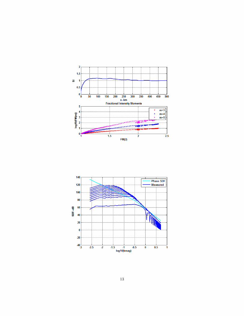
selection of the output �le, the following three �gures are generated. Theupper frame of Figure 2.1.1 (book Figure 3.12) shows the scintillation index asa function of distance. The theory predicts a monotonic increase to saturation(SI = 1). The fact that the measured index exceeds unity by a small amountis a statistical uctuation. The lower frame shows intensity moments 3, 4and 5, normalized to the second intensity moment. Thus, FM(2) = SI2 + 1.The pentagrams indicate the fractional moment for exponentially distributed(Rayleigh) intensity uctuations FM(m) = m!. Although the SI index isclose to unity, the higher order fractional moments indicate a departure fromRayleigh statistics. Figure 2.1.1 (book Figure 3.1.3) shows the evolutionof the intensity radial wavenumber spectrum with an overlay of the theoreticalphase radial wavenumber SDF for reference. The power-law tail portion of theintensity spectrum has the same slope and in this case coincides with the phaseSDF.Figures 2.1.1 and 2.1.1 (book Figures 3.21 and 3.22) show, respectively, the

intensity �eld and power spectrum of the complex �eld. One can see �laments inthe intensity structure that suggest signi�cant departure from speckle (Rayleighdistributed uctuations). The SDF of the complex �eld shows a bright central

3

4

(low spatial frequency) region sitting on a plateau. Recovering the underlyingphase spectrum from the output would be very di�cult, as discussed in Chapter3.

2.1.2 Large Slope

To run the large-slope example transfer the active MATLAB directory to

� � �nPropCode2 ExamplesnLargeSlope

and run SetupPropCode2. Next run PropCode2 to generate the output complex�eld as before. The following 3 �gures can be generated by executing the scriptRunDisplayPropCode2Out as before. Figure 2.1.2 (book Figure 3.14) shows theevolution of the scintillation index (upper frame) and the fractional moments(lower frame). The tendency of the intensity statistics to converge to Rayleighis a predicted result described in Chapter 3 of the book. Figures 2.1.2 and 2.1.2(book Figures 3.23 and 3.24) show, respectively, the intensity �eld and powerspectrum of the complex �eld at the maximum distance.

2.1.3 Strong Focusing

To run the strong-focusing example transfer the active MATLAB directory to

� � � nPropCode2 ExamplesnStrongFocusing

5

6

7

8

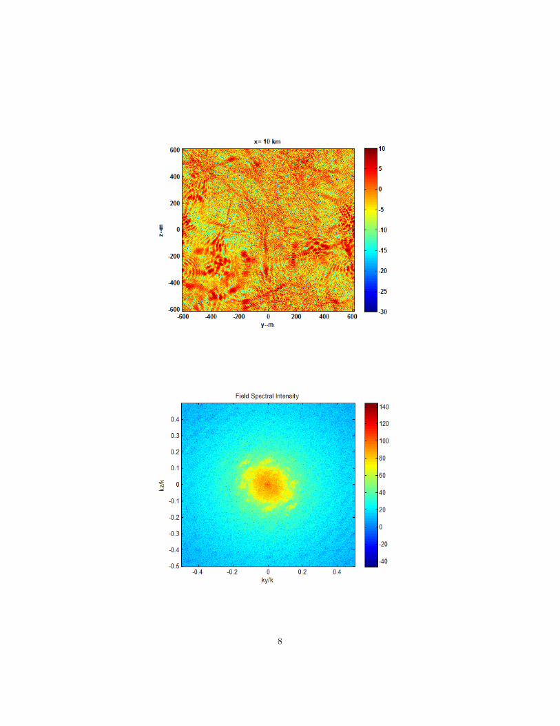
and run SetupPropCode2. Running PropCode2 followed by DisplayPropCode2Outwill reproduce Figures 2.1.3 (book Figure 3.16) and 2.1.3. Figure 2.1.3 showsthe evolution of the SI index, which achieves its maximum value at 265 m fromthe phase screen. Subsequent propagation to 10 km shows that the statisticshave converged to Rayleigh as predicted by theory. Figure 2.1.3 shows the veryhomogenous distribution of the intensity distribution. As theory predicts, thereis an initial pronounced departure from Rayleigh statistics, but if the propaga-tion distance is increased signi�cantly enough, the intensity statistics becomespeckle like.A second simulation initiated with SetupPropCode2a followed by PropCode2

will terminate the computation at the distance where SI achieves its maximumvalue. Executing DisplayPropCode2Out with GUI selection of the second runwill generate the following �gures (book Figures 3.25 and 3.26), the latter ofwhich is a dramatic example of strong focusing.

2.1.4 Strong Focusing Movie

The movie example can be found in the folder

� � � nPropCode2 ExamplesnStrongFocusingMOV

Executing the setup utility followed by an execution of PropCode2 will generatethe output. The display utility is con�gured to generate an .avi movie �le.

9

10

11

2.1.5 Two-Slope

An SDF with two power-law segments is a more exible model. Running thescript SetupPropCode2 in the directory

� � � nPropCode2 ExamplesnTwoSlope

will generate the a *.mat �le for the two component power law shown inFig 2.1.5, which can be reproduced by executing ReadSetupFile2. RunningPropCode2 followed by DisplayPropCode2Out will reproduce Figures 2.1.5 and2.1.5.

12

13