Earth Syst. Dynam., 6, 461–484, 2015

www.earth-syst-dynam.net/6/461/2015/

doi:10.5194/esd-6-461-2015

© Author(s) 2015. CC Attribution 3.0 License.

Propagation of biases in humidity in the estimation of

global irrigation water

Y. Masaki, N. Hanasaki, K. Takahashi, and Y. Hijioka

National Institute for Environmental Studies, 16-2 Onogawa, Tsukuba, Ibaraki, 305-8506, Japan

Correspondence to: Y. Masaki (masaki.yoshimitsu@nies.go.jp)

Received: 25 December 2014 – Published in Earth Syst. Dynam. Discuss.: 26 January 2015

Revised: 4 June 2015 – Accepted: 5 June 2015 – Published: 20 July 2015

Abstract. Future projections on irrigation water under a changing climate are highly dependent on meteorolog-

ical data derived from general circulation models (GCMs). Since climate projections include biases, bias correc-

tion is widely used to adjust meteorological elements, such as the atmospheric temperature and precipitation, but

less attention has been paid to biases in humidity. Hence, in many cases, uncorrected humidity data have been di-

rectly used to analyze the impact of future climate change. In this study, we examined how the biases remaining

in the humidity data of five GCMs propagate into the estimation of irrigation water demand and consumption

from rivers using the global hydrological model (GHM) H08. First, to determine the effects of humidity bias

across GCMs, we ran H08 with GCM-based meteorological forcing data sets distributed by the Inter-Sectoral

Impact Model Intercomparison Project (ISI-MIP). A state-of-the-art bias correction method was applied to the

data sets without correcting biases in humidity. Differences in the monthly relative humidity amounted to 11.7

to 20.4 % RH (percentage relative humidity) across the GCMs and propagated into differences in the estimated

irrigation water demand, resulting in a range between 1152.6 and 1435.5 km3 yr−1 for 1971–2000. Differences

in humidity also propagated into future projections. Second, sensitivity analysis with hypothetical humidity bi-

ases of ±5 % RH added homogeneously worldwide revealed the large negative sensitivity of irrigation water

abstraction in India and East China, which are heavily irrigated. Third, we performed another set of simulations

with bias-corrected humidity data to examine whether bias correction of the humidity can reduce uncertainties

in irrigation water across the GCMs. The results showed that bias correction, even with a primitive methodology

that only adjusts the monthly climatological relative humidity, helped reduce uncertainties across the GCMs: by

using bias-corrected humidity data, the uncertainty ranges of irrigation water demand across the five GCMs were

successfully reduced from 282.9 to 167.0 km3 yr−1 for the present period, and from 381.1 to 214.8 km3 yr−1 for

the future period (RCP8.5, 2070–2099). Although different GHMs have different sensitivities to atmospheric

humidity because different types of potential evapotranspiration formulae are implemented in them, bias correc-

tion of the humidity should be applied to forcing data, particularly for the evaluation of evapotranspiration and

irrigation water.

1 Introduction

Recent ongoing global warming is expected to change cur-

rent hydroclimatological environments at the global scale.

Since fresh water is essential for various industrial and so-

cial activities of human beings, its availability plays a crucial

role in the sustainable development of society.

Agriculture is one of the human activities that are highly

susceptible to hydroclimatological conditions. Irrigated wa-

ter is supplied to cropland to compensate for the deficit in the

soil water content, which affects crop growth. Since soil wa-

ter is primarily consumed through evapotranspiration, which

is sensitive to meteorological conditions, the amount of re-

quired irrigation water varies with the meteorological con-

ditions. According to Vörösmarty et al. (2005) (Tables 7.3

and 7.4), the total amount of global freshwater withdrawal

was 3560 km3 yr−1 for 1995–2000, 2480 km3 yr−1 (70 % of

the total withdrawal) of which was supplied for agricultural

Published by Copernicus Publications on behalf of the European Geosciences Union.

462 Y. Masaki et al.: Estimation of global irrigational water

use, and the consumption through evapotranspiration from

irrigated cropland amounted to 1210 km3 yr−1 (34 % of the

total human withdrawal and 49 % of the total agricultural

withdrawal). In Asia, a larger proportion of abstracted water

is consumed through evapotranspiration (52 % of the total

human withdrawal and 59 % of the total agricultural with-

drawal) than the global average. Moreover, the volume of ir-

rigation water is expected to increase in the future because

of an increase in evapotranspiration from cropland under

warmer climates (e.g., Wada et al., 2013) and the expan-

sion of irrigated cropland to meet the increasing demand for

food owing to the increase in the world population (e.g., Bru-

insma, 2011; Elliott et al., 2014). Precise estimation of the

amount of irrigation water abstraction is crucial for the sus-

tainable use of available water in the future.

To quantitatively evaluate future irrigation water, we must

substantially rely on hydrological simulation. However, there

are fundamental difficulties in the estimation because there

are many possible errors and uncertainties in the data sets

(meteorological data sets, land use data, etc.), calculation

schemes (evapotranspiration, runoff, river flow, etc.) and pa-

rameters. Moreover, there are also difficulties in incorpo-

rating irrigation schemes that are able to represent realistic

irrigation management and performance. In fact, different

general circulation models (GCMs) and global hydrological

models (GHMs) give different estimates. Wisser et al. (2008)

showed that the discrepancies in the estimation stem from

both meteorological and irrigated area data. Recently, the

Inter-Sectoral Impact Model Intercomparison Project (ISI-

MIP) set the estimation of uncertainties in both GCMs and

GHMs through intermodel comparison as one of its goals

(Warszawski et al., 2014).

GCM biases are one of the substantial sources of uncer-

tainty in future climate projections. For over a decade, we

have made considerable effort to remove GCM biases from

the temperature and precipitation data because these mete-

orological elements are crucial for analyzing the impact of

climate change. However, hydrological simulations require

other meteorological elements in addition to these elements.

Solving water and heat budgets at the ground surface basi-

cally requires seven meteorological elements (atmospheric

temperature, precipitation, short- and longwave downward

radiation, wind velocity, pressure and humidity). Less atten-

tion has been paid to GCM biases of meteorological elements

other than temperature and precipitation. Haddeland et al.

(2012) intensively examined the compound effects of the bias

correction of radiation, wind and humidity, and showed that

bias correction has an impact on absolute values of evapo-

transpiration but less impact on relative changes. Moreover,

global humidity observation data sets contain uncertainties

originating from the accuracy of measurements, grid sam-

pling (Willett et al., 2013) and the spatial variability within

land cells. Knowing the sensitivity of irrigation water to hu-

midity conditions at different locations would help clarify the

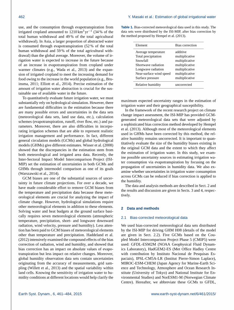
Table 1. Bias-corrected meteorological data used in this study. The

data sets were distributed by the ISI-MIP, after bias correction by

the method proposed by Hempel et al. (2013).

Element Bias correction

Average temperature additive

Total precipitation multiplicative

Snowfall multiplicative

Shortwave radiation multiplicative

Longwave radiation multiplicative

Near-surface wind speed multiplicative

Surface pressure multiplicative

Relative humidity uncorrected

maximum expected uncertainty ranges in the estimation of

irrigation water and their geographical susceptibility.

In the framework of the recent research project on climate

change impact assessment, the ISI-MIP has provided GCM-

generated meteorological data sets that were adjusted by

a sophisticated bias correction method developed by Hempel

et al. (2013). Although most of the meteorological elements

used in GHMs have been corrected by this method, the rel-

ative humidity remains uncorrected. It is important to quan-

titatively evaluate the size of the humidity biases existing in

the original GCM data and the extent to which they affect

the estimation of irrigation water. In this study, we exam-

ine possible uncertainty sources in estimating irrigation wa-

ter consumption via evapotranspiration by focusing on the

propagation of uncertainties in humidity data. We also ex-

amine whether uncertainties in irrigation water consumption

across GCMs can be reduced if bias correction is applied to

the humidity.

The data and analysis methods are described in Sect. 2 and

the results and discussion are given in Sects. 3 and 4, respec-

tively.

2 Data and methods

2.1 Bias-corrected meteorological data

We used bias-corrected meteorological data sets distributed

by the ISI-MIP for driving GHM H08 (details of the model

are given in Sect. 2.2). Five GCMs based on the Cou-

pled Model Intercomparison Project Phase 5 (CMIP5) were

used: GFDL-ESM2M (NOAA Geophysical Fluid Dynam-

ics Laboratory), HadGEM2-ES (Met Office Hadley Centre

with contribution by Instituto Nacional de Pesquisas Es-

paciais), IPSL-CM5A-LR (Institut Pierre-Simon Laplace),

MIROC-ESM-CHEM (Japan Agency for Marine-Earth Sci-

ence and Technology, Atmosphere and Ocean Research In-

stitute (University of Tokyo) and National Institute for En-

vironmental Studies) and NorESM1-M (Norwegian Climate

Centre). Hereafter, we abbreviate these GCMs to GFDL,

Earth Syst. Dynam., 6, 461–484, 2015 www.earth-syst-dynam.net/6/461/2015/

Y. Masaki et al.: Estimation of global irrigational water 463

HadGEM, IPSL, MIROC and NorESM, respectively. Bias

correction was applied to the meteorological elements listed

in Table 1 using the method of Hempel et al. (2013) with

observation-based WATCH meteorological data sets (Wee-

don et al., 2011) for 1960–1999. The bias in relative humid-

ity in the GCMs has remained uncorrected because of diffi-

culties in preserving physical consistency between humidity-

related variables (relative/specific humidity, vapor pressure),

the atmospheric temperature and the pressure after bias cor-

rection (ISI-MIP, 2012). The geographical resolution of all

meteorological data was commonly adjusted to 0.5◦× 0.5◦.

Future projections were made under four representative con-

centration pathways (RCPs 2.6, 4.5, 6.0 and 8.5) (Moss et al.,

2010; van Vuuren et al., 2011).

2.2 Hydrological model

The hydrological model used in this study was H08

(Hanasaki et al., 2008a, b). The model solves both the wa-

ter and energy balances at a time step of 1 day with global

coverage at a resolution of 0.5◦× 0.5◦. The model consists

of six submodels (land surface hydrology, river routing, crop

growth, water abstraction, reservoir operation and environ-

mental flow requirement), but only the first four submodels

were employed in this study. The land surface hydrology sub-

model solves the water and energy balances. The submodel

solves the water balance using simple and basic physical hy-

drological processes that are suitable for global-scale sim-

ulation. A 1 m leaky bucket is assumed in the model: the

soil moisture in each land cell is expressed as water stored

in this bucket, and the water slowly drains from the bucket

to express the subsurface runoff. The crop growth submodel

is a process-based model that is used to estimate the crop-

growing season globally. The water abstraction submodel es-

timates the human impacts of irrigational, municipal and in-

dustrial water abstraction from rivers for consumptive use.

The consumptive use of irrigation water was estimated from

the deficit in the soil water content compared with a target

level in irrigated cropland during the growing season. Details

are described in the second half of this section. The water is

abstracted from rivers as the first choice if the riverine water

is available; the rest of the required water is limitlessly sup-

plied from non-renewable and non-local blue water resources

(e.g., groundwater or long-distance transported water; see

Rost et al., 2008; Hanasaki et al., 2010). Values for the con-

sumptive use of municipal and industrial water were taken

from country-based AQUASTAT data (FAO, 2015). Munici-

pal and industrial water consumption at each land cell were

weighted by the population using the Gridded Population of

the World, version 3 (GPWv3) (CIESIN and CIAT, 2005).

Socioeconomic conditions (e.g., the population and irrigated

area) were fixed at those in the year 2000. To stabilize the

initial conditions, the hydrological model was spun up using

data from 1950 to 1959.

We assumed that irrigation water is supplied to irrigated

cropland under the condition that crops are not affected by

water stress. The soil water content was maintained at 75 %

of the field capacity for all crops except rice (100 %) dur-

ing the growing season and for 30 days before the planting

date. If there is a deficit relative to this threshold, soil wa-

ter content was assumed to be supplied by irrigation. The

soil water of cropland is consumed through evapotranspi-

ration and lost through runoff. The former was calculated

from both the meteorological conditions and the soil water

content (see Sect. 2.3), whereas the latter was assumed to

vary with the soil water content. The spatial distribution of

the irrigated area was fixed at that for the year 2000 based

on the data of Siebert et al. (2005) throughout the analysis

period. We separately calculated the results for three differ-

ent water management schemes corresponding to three types

of agricultural land use: double-cropping irrigated cropland

(we refer to this water management scheme as Mosaic 1

hereafter), single-cropping irrigated cropland (Mosaic 2) and

rain-fed cropland (Mosaic 3). Their geographical distribu-

tions are shown in Fig. 1. Information on double and single

croppings was taken from the cropping intensity reported by

Döll and Siebert (2002). We aggregated the three types of

water management into a land cell (Mosaic 0) in considera-

tion of their areal fractions in each land cell. We considered

the 19 crops (18 crops plus “others”) used in Table 7 in Leff

et al. (2004) but with an updated geographical distribution

for the year 2000 (Monfreda et al., 2008). The crop parame-

ters used to calculate their growth were based on the SWIM

code (Krysanova et al., 2000).

In this study, we evaluated two quantities regarding the ir-

rigation water (hereafter, the water volume is reported on a

consumption basis): irrigation water demand (IWD) and ir-

rigation water consumption from rivers (IWCR). The IWD

gives the cumulative amount of water to be supplied over

cropland to compensate for the deficit relative to a thresh-

old soil water content. The soil water is primarily supplied

by precipitation under natural conditions and consumed via

evapotranspiration, drained by runoff and so forth. Since we

assumed that the soil water should be kept at a certain level

by irrigation (described in Sect. 2.3 in detail), IWD gives the

additional amount of water required to prevent crops from

suffering water stress under given meteorological conditions.

In other words, the IWD gives the maximum water consump-

tion while maintaining the current agricultural maneuver (ge-

ographical distribution of irrigated cropland, cultivars, water

management in irrigated cropland, etc.) under idealized con-

ditions without fear of water shortage.

The IWCR gives the irrigation water consumption that

can be supplied from rivers and is defined as a proportion

of the IWD. In practice, irrigation water is abstracted from

various resources (e.g., rivers, local reservoirs, groundwater).

Among them, rivers are the largest water resource and their

flow is vulnerable to future climate change. Thus, it is impor-

tant to examine the proportion of IWD that can be supplied

www.earth-syst-dynam.net/6/461/2015/ Earth Syst. Dynam., 6, 461–484, 2015

464 Y. Masaki et al.: Estimation of global irrigational water

Figure 1. Geographical distribution of irrigated croplands – (a) double cropping each year (Mosaic 1), (b) single cropping each year

(Mosaic 2) and (c) rain-fed cropland (Mosaic 3) – used in this study. The distributions are indicated in black.

from rivers. By taking this situation into consideration, our

calculation scheme was based on the assumption that water

is primarily abstracted from rivers (Hanasaki et al., 2010).

Through evaluation of IWCR under restrictions of riverine

water availability, we estimated the extent to which humidity

biases affect hydrological variables that are not determined

only from meteorological conditions.

2.3 Evapotranspiration calculation scheme

Various formulae for estimating potential evapotranspiration

have been developed (e.g., Shelton, 2009), and researchers

have utilized suitable formulae for their own research pur-

poses. These formulae are classified into two basic cate-

gories: physical and empirical formulae. The former describe

potential evapotranspiration from the viewpoint of the energy

balance at the land surface, and such formulae are suitable

for (micro)meteorological studies requiring a high temporal

resolution. Thus, this type of formula requires several mete-

orological elements such as the surface temperature, humid-

ity, radiation and wind speed. On the other hand, the latter

describe climatological conditions for less time-varying phe-

nomena in a simplified manner and, in general, require only

two or three meteorological elements. Thus, the latter are

suitable for sites where meteorological observation data are

limited. Examples of evapotranspiration formulae are given

in the Appendix.

The calculation scheme for potential evapotranspiration

Epot employed in H08 is the bulk formula (Kondo, 1994)

Epot = ρCDU (qsat(Ts)− q), (1)

where ρ, CD and U are the air density, bulk transfer coef-

ficient (0.003) and wind speed, respectively. Thus, Epot is

proportional to the difference between the saturated specific

humidity at the surface temperature qsat(Ts) and the specific

humidity of the air q. Since bias correction was indepen-

dently applied to each meteorological element except for the

relative humidity, the physical consistency among meteoro-

logical elements guaranteed in the original GCMs might be

lost. In this study, we recalculated q to maintain local phys-

ical consistency between the bias-corrected temperature and

uncorrected relative humidity.

Actual evapotranspiration is estimated by multiplying by

a function of the soil water contentW . IfW is less than three-

quarters of the field capacityWfc,Eact linearly decreases with

decreasing W :

Eact = βEpot, (2)

where

β =

{1 (W ≥ 0.75Wfc)

W0.75Wfc

(W < 0.75Wfc). (3)

The soil water content in irrigated cropland was assumed to

be maintained at 0.75Wfc (Wfc for rice) to prevent crops from

suffering water stress. That is, evapotranspiration from irri-

gated cropland is not suppressed by a decrease in the soil

water content (i.e., Eact = Epot) during the growing season.

Although the actual threshold may be different for different

types of irrigation (e.g., sprinklers, drip irrigation, ditch irri-

gation) or irrigation management, global information on such

variation is unavailable. The adopted irrigation scheme based

on the soil water content is simple but applicable for global-

scale simulations (e.g., Döll and Siebert, 2002).

Earth Syst. Dynam., 6, 461–484, 2015 www.earth-syst-dynam.net/6/461/2015/

Y. Masaki et al.: Estimation of global irrigational water 465

2.4 Experiment design of this study

To investigate the effects of bias correction of the humid-

ity, we designed three sets of experiments in this study: (1)

a reference experiment, (2) a sensitivity experiment and (3)

a bias-corrected experiment. In the reference experiment,

a hydrological simulation was performed with the uncor-

rected humidity data described in Sect. 2.1. We evaluated the

evapotranspiration and irrigation water for both present and

future periods. The results were also used as a reference for

the other two sets of experiments, details of which are given

below.

2.4.1 Sensitivity experiment with hypothetical bias in

humidity

Measurement of the atmospheric humidity inevitably in-

volves errors. Observation-based humidity data sets, which

are often used as reference data for bias correction, might

contain a certain level of error. Moreover, the sensitivity

of the amount of irrigation water to atmospheric humidity

varies geographically or seasonally because irrigation wa-

ter depends not only on meteorological conditions but also

on the areal fraction of irrigated cropland, irrigation man-

agement, irrigation techniques and the cultivation maneuver

(crop type, crop calendar, etc.) in each land cell.

To evaluate the sensitivity of the amount of irrigation water

to atmospheric humidity, we carried out a sensitivity exper-

iment in which we introduced a pair of constant biases so

that the data were higher and lower than the original GCM-

based humidity data and investigated the effect of the biases

on irrigation water. The sensitivity is also helpful for pre-

dicting the size of the error in the simulation of irrigation

water. In this experiment, we introduced “hypothetical” bi-

ases into the relative humidity by simply adding biases of

±5 % RH as a worst case (discussed below) homogeneously

to all the land cells. (Hereafter, to discriminate between the

unit of relative humidity and a general percentage, we use

% RH for the unit of humidity.) When the relative humidity

exceeded 100 % RH or became negative, we used values of

100 and 0 % RH, respectively. The other meteorological ele-

ments were unchanged. This experiment was carried out for

the both present and future periods.

In fact, Willett et al. (2013) reported that the maximum un-

certainties in humidity measurements with dry- and wet-bulb

thermometers amounted to 2.75 and 5 % RH at temperatures

of 0 and−10 ◦C, respectively. Emeis (2010) summarized the

errors for various measurement equipment: for example, ad-

vanced equipment based on the capacitive method has an ac-

curacy of 2 % RH (for a humidity of 10–80 % RH) to 3 % RH

(for a humidity of 80–ca. 100 % RH). By considering these

reports, we set ±5 % RH as the worst case in this study.

Through such sensitivity experiments, we are able to esti-

mate the largest possible ranges of uncertainty in irrigation

water consumption due to an uncertainty in the relative hu-

midity of α% RH because the uncertainty for irrigation water

in the case of geographically random biases within±α% RH

necessarily lies between those for the two extremes of the

globally homogeneous bias of ±α% RH. Recall that, be-

cause of the supply of irrigation water, Eact = Epot for irri-

gated cropland during the growing season. If we artificially

add positive (negative) biases to the relative humidity with-

out changing other elements, both ρ and qsat(Ts)− q on the

right-hand side of the bulk formula (Eq. 1) will decrease (in-

crease), resulting in a decrease (increase) in potential eva-

potranspiration. The increase in Epot via qsat(Ts)1 is smaller

than the direct decrease in Epot resulting from introducing

a hypothetical bias of α% RH. Therefore, Eact has a mono-

tonic dependence on the humidity bias:Eact becomes smaller

(larger) for positive (negative) biases in the relative humidity.

We note that this simple relation holds only for irri-

gated cropland during the crop-growing season when irri-

gation water is limitlessly supplied. In rain-fed cropland or

irrigation-free seasons, evapotranspiration has a complex de-

pendence on meteorological conditions (Wang and Dickin-

son, 2012) because Eact also depends on the soil moisture

content (Eq. 3).

The sensitivity experiment was also carried out for a fu-

ture period because different GCMs project different fu-

ture climates. Even if the biases in meteorological elements

were completely removed for the present period, the fu-

ture temperature or precipitation would still differ across the

GCMs. Since evapotranspiration is also sensitive to temper-

ature conditions, the future sensitivity may be different from

the present sensitivity and also vary among the GCMs. The

sensitivity experiment for a future period will help clarify the

propagation of humidity biases into the amount of irrigation

water even under different future climates projected by dif-

ferent GCMs.

2.4.2 Bias-corrected experiment

If we introduce bias correction of the humidity, does it af-

fect hydrological projections and have any advantages? To

examine this effect, we prepared another set of meteorologi-

cal data for which the humidity data were bias-corrected with

a primitive methodology that adjusts only the monthly cli-

matology. Using this bias-corrected humidity data set and

the original bias-corrected meteorological data sets for the

other elements, we recalculated the hydrological process in

the same way and compared the results with the uncorrected

ones (i.e., those of the reference experiment). This experi-

ment was carried out for both the present and future periods.

The bias correction methodology was based on additive

adjustment in order to preserve the range of variability in the

1A decrease (increase) in potential evapotranspiration will in-

crease (decrease) Ts owing to the prevention (promotion) of cooling

by latent heat, and result in an increase (decrease) in Epot through

an increase (decrease) in qsat(Ts).

www.earth-syst-dynam.net/6/461/2015/ Earth Syst. Dynam., 6, 461–484, 2015

466 Y. Masaki et al.: Estimation of global irrigational water

Table 2a. Total number of days when the humidity is oversaturated (> 100 % RH) in the original regridded GCM data. Both the annual and

seasonal sums are given as the mean over all land cells (67 420 cells). The total numbers of days are given in parentheses in the header.

GCMs 1971–2000 2070–2099 RCP8.5

Annual DJF MAM JJA SON Annual DJF MAM JJA SON

(10 958) (2708) (2760) (2760) (2730) (10 957) (2707) (2760) (2760) (2730)

GFDL-ESM2M 715.6 330.4 99.0 20.8 265.5 692.4 342.5 87.9 27.9 234.1

HadGEM2-ES 738.6 416.1 165.5 10.1 146.9 417.8 263.7 78.9 3.1 72.2

IPSL-CM5A-LR 0.0 0.0 0.0 0.0 0.0 0.0 0.0 0.0 0.0 0.0

MIROC-ESM-CHEM 636.8 310.9 187.9 14.6 123.3 228.5 122.7 62.8 12.8 30.2

NorESM1-M 290.9 169.7 48.7 0.5 72.0 130.0 91.7 20.5 0.8 16.8

Ensemble mean 476.4 245.4 100.2 9.2 121.5 293.7 164.1 50.0 8.9 70.7

Table 2b. Total number of days when the humidity is truncated at 100 % RH during adjustment by our primitive bias correction described in

Sect. 2.4.2. Both the annual and seasonal sums are given by the mean over all land cells (67 420 cells). The total numbers of days are given

in parentheses in the header.

GCMs 1971–2000 2070–2099 RCP8.5

Annual DJF MAM JJA SON Annual DJF MAM JJA SON

(10 958) (2708) (2760) (2760) (2730) (10 957) (2707) (2760) (2760) (2730)

GFDL-ESM2M 526.7 256.0 117.8 37.5 115.4 563.0 280.6 115.6 49.9 116.8

HadGEM2-ES 528.2 313.4 89.9 11.6 113.2 333.1 202.4 52.7 10.1 67.7

IPSL-CM5A-LR 186.2 92.3 32.2 27.9 33.8 141.0 72.5 24.3 20.9 23.3

MIROC-ESM-CHEM 411.6 245.6 74.5 7.3 84.3 170.5 99.4 27.8 10.7 32.5

NorESM1-M 277.2 167.2 41.8 10.0 58.2 159.9 103.9 23.7 7.9 24.3

Ensemble mean 386.0 214.9 71.2 18.9 81.0 273.5 151.8 48.8 19.9 52.9

relative humidity because the evapotranspiration obtained by

a physical formula (see Appendix) is sensitive to the vapor

pressure deficit. First, we obtained the monthly climatolog-

ical relative humidity at all land cells for each GCM by av-

eraging the relative humidity data for the same month of the

year over the period 1960–1999. By subtracting the monthly

climatological relative humidity in the GCM for the same

period from those in the WATCH observational data, we

determined the climatological monthly adjustments. Then,

we compiled daily bias-corrected humidity data by simply

adding the climatological monthly adjustments to the orig-

inal GCM daily humidity data. Values of less than 0 % RH

and greater than 100 % RH were set to 0 and 100 % RH, re-

spectively.

We summarize the statistics of the truncated humidity data

before and during our bias correction in Table 2. The orig-

inal regridded data already contain supersaturation (greater

than 100 % RH), except for IPSL (Table 2a). Most of the su-

persaturation data were obtained at high northern latitudes in

winter where the atmospheric temperature was well below

0 ◦C. The number of truncated humidity data at 100 % RH

during our primitive bias correction (Table 2b) is less than the

number of supersaturation data in the original regridded data

except for IPSL, particularly in the boreal winter, because

a certain proportion of the oversaturated data in the GCMs

were adjusted to undersaturated data by the bias correction

when the monthly climatological humidity of the GCMs was

larger than that of the WATCH data. In contrast, the num-

ber of truncated humidity data at 0 % RH is very small (Ta-

ble 2c). These truncations were observed in highly dry re-

gions, such as deserts. Generally, the number of truncated

data at 100 % RH in the future projection (RCP8.5) is smaller

than that in the present, whereas the number at 0 % RH is

larger than the present number.

We expect the errors in evapotranspiration due to these

truncations to be marginal and not to cause major problems in

the interpretation of our results on hydrological variables. In

fact, the evapotranspiration under the low-temperature con-

ditions typically seen at high northern latitudes in winter ap-

proaches zero. Moreover, few crops are cultivated in the win-

ter, and irrigated agriculture is not practiced in these regions.

Similarly, evapotranspiration in and around desert areas (ex-

cept in limited areas with intensive irrigation) is also very

small.

Earth Syst. Dynam., 6, 461–484, 2015 www.earth-syst-dynam.net/6/461/2015/

Y. Masaki et al.: Estimation of global irrigational water 467

Table 2c. Total number of days when the humidity is truncated at 0 % RH during adjustment by our primitive bias correction described in

Sect. 2.4.2. Both the annual and seasonal sums are given by the mean over all land cells (67 420 cells). The total numbers of days are given

in parentheses in the header.

GCMs 1971–2000 2070–2099 RCP8.5

Annual DJF MAM JJA SON Annual DJF MAM JJA SON

(10 958) (2708) (2760) (2760) (2730) (10 957) (2707) (2760) (2760) (2730)

GFDL-ESM2M 28.34 3.19 7.53 10.42 7.20 39.35 4.25 10.25 15.35 9.51

HadGEM2-ES 2.34 0.11 1.34 0.38 0.49 5.20 0.39 2.56 1.31 0.95

IPSL-CM5A-LR 1.03 0.04 0.61 0.19 0.19 4.94 0.74 2.50 0.80 0.90

MIROC-ESM-CHEM 7.79 1.23 2.01 2.04 2.50 17.21 2.63 4.98 3.65 5.95

NorESM1-M 10.62 2.61 3.82 2.45 1.74 18.80 2.80 9.46 4.43 2.11

Ensemble mean 10.02 1.44 3.06 3.10 2.42 17.10 2.16 5.95 5.11 3.88

Table 3. Global average of monthly SD ( % RH) in relative humidity, shown in Fig. 4, for each land use.

GCMs Mosaic 0 Mosaic 1 Mosaic 2 Mosaic 3

GFDL-ESM2M 20.3 26.2 23.9 17.6

HadGEM2-ES 11.7 24.3 20.1 13.4

IPSL-CM5A-LR 15.0 34.8 27.0 13.6

MIROC-ESM-CHEM 20.4 18.0 20.0 17.4

NorESM1-M 17.9 20.4 18.8 13.4

3 Results

3.1 Comparison of performance of meteorological

elements between GCMs

We first examine the differences in the meteorological ele-

ments between the five GCMs in the framework of the ref-

erence experiment to search for existing GCM-inherent bi-

ases and compare them with the WATCH observation-based

meteorological elements to evaluate the performance of bias

correction. Figure 2 shows the monthly difference worldwide

averaged over each type of land use (mosaic). Monthly pro-

files of the atmospheric temperature, precipitation and short-

wave downward radiation for the five GCMs agree with those

of WATCH. Note that the 30-year analysis period (1971–

2000) is slightly different from the bias correction period

(1960–1999). For the wind speed data, although the monthly

profile of MIROC is slightly larger than that of WATCH over

Mosaic 1, we consider the overall performance of bias cor-

rection to be reasonably good for the wind data.

In contrast, the monthly profiles of the relative humidity,

which contain GCM-inherent biases, show a large disper-

sion between the five GCMs and also deviate from those of

WATCH. The global-mean relative humidity over Mosaic 1

shows a larger dispersion than those over the other mosaics:

the largest difference in the relative humidity between the

monthly GCMs reaches 19.8 % RH in both January and Oc-

tober with a minimum of 11.0 % RH in May for Mosaic 1.

Such differences in the uncorrected relative humidity

cause the deviation of the potential evapotranspiration

and evapotranspiration between the five GCMs. Figure 3

shows their monthly profiles. Different GCMs have differ-

ent monthly profiles and peak months. The difference in the

potential evapotranspiration among the GCMs for Mosaic 1

reaches a maximum of 1.23 mmday−1 in June with a mini-

mum of 0.56 mmday−1 in December. The difference exceeds

0.9 mmday−1 from March to October. Since the temperature,

shortwave downward radiation and wind speed, which are re-

quired for the calculation of the potential evapotranspiration

(Eq. 1), are successfully bias-corrected (Fig. 2), these differ-

ences in the potential evapotranspiration are considered to be

mainly due to GCM biases in the relative humidity. NorESM

tends to have a small but positive bias of the potential evapo-

transpiration and a small negative bias of the evapotranspi-

ration during the summer. However, no clear biases of the

relative humidity can be observed in Fig. 2.

Next, we determine the geographical distribution of the

GCM biases with respect to the WATCH data because re-

gional deviations with opposite signs may cancel each other

when calculating the global mean. Figures 4, 5 and 6 show

the SD of 12-month climatological data of the relative hu-

midity, atmospheric temperature and precipitation of the

GCMs with respect to the WATCH data, respectively. Strong

regional patterns were detected in the relative humidity

(Fig. 4). Figure 4 also shows that the relative humidity in

high mountainous areas (Rocky Mountains, Andes and Hi-

malayas) have larger deviations from the WATCH data for

all GCMs. Each GCM has a different geographical distribu-

tion. For example, GFDL exhibits large differences over the

www.earth-syst-dynam.net/6/461/2015/ Earth Syst. Dynam., 6, 461–484, 2015

468 Y. Masaki et al.: Estimation of global irrigational water

−10

0

10

20

30

Atm

os. T

emp.

[C−

deg]

Mosaic 0

Tair (1971−2000)

0

2

4

6

8

10

Pre

cipi

tatio

n (t

otal

) [m

m/d

ay]

Prcp (1971−2000)

40

50

60

70

80

Rel

ativ

e hu

mid

ity [%

]

Rh (1971−2000)

0

10

20

30

Sho

rtw

ave

rad.

[MJ/

day/

m2 ]

SWdown(1971−2000)

1

2

3

4

Win

d ve

l. [m

/s]

1 2 3 4 5 6 7 8 9101112

Month

Wind(1971−2000)

Mosaic 1

1 2 3 4 5 6 7 8 9101112

Month

Mosaic 2

1 2 3 4 5 6 7 8 9101112

Month

Mosaic 3

1 2 3 4 5 6 7 8 9101112

Month

GFDLHadGEMIPSL

MIROCNorESMWFD

Figure 2. Monthly profiles of meteorological elements used in this

study for 1971–2000. The results are aggregated over each type of

land use, identified by the mosaic number. Profiles of the five GCMs

are indicated in different colors: (red) GFDL, (green) HadGEM,

(blue) IPSL, (dark yellow) MIROC and (light blue) NorESM. Pro-

files of the WATCH data are shown as black lines with dots.

world. HadGEM and IPSL have large differences in Eurasia

but good performance in Australia. MIROC has high devia-

tions in inland regions of Asia and Australia. NorESM has

small differences in Europe and the eastern United States but

large differences in Australia.

In contrast, uniformly distributed small biases (less than

0.5 ◦C for most of the world) were observed for the tem-

perature (Fig. 5). The SD for the precipitation (Fig. 6) is

less than 0.2 mmday−1 for most of the world and around

0.5 mmday−1 for humid areas (e.g., Southeast Asia). Al-

though exceptions are seen in the Amazonian inland, where a

large SD is observed for GFDL and IPSL, these contributions

are considered to be marginal when taking the large annual

precipitation (greater than 2000 mm) and the smaller amount

of cropland (see Fig. 1) into account. These results also indi-

cate that the bias corrections of the atmospheric temperature

and precipitation were successful at the regional scale.

We averaged the monthly SD over the land cells of each

mosaic and summarized the results in Table 3. HadGEM has

the smallest deviation from WATCH over all land cells (Mo-

saic 0). However, MIROC and NorESM have superior per-

formance for Mosaic 1 and 2. Since both Mosaic 1 and 2 are

irrigated cropland, differences in the potential evapotranspi-

ration directly affect differences in the amount of irrigation

water. Errors in the humidity are one possible error source

when calculating evapotranspiration. In this sense, small hu-

midity biases over irrigated cropland are beneficial for sup-

pressing their effects on irrigation water provided that other

meteorological elements are successfully bias-corrected.

3.2 GCM features and their propagation into future

projections

Next, we examine the extent to which GCM-inherent fea-

tures in the relative humidity affect the estimation of irriga-

tion water and propagate into a future period (2070–2099)

in the framework of the reference experiment. If the effects

are not negligible, bias correction of the humidity, as well as

other meteorological elements, is highly recommended.

Figure 7 shows future monthly profiles of the five GCMs.

Since the meteorological variables are bias-corrected for

1960–1999, the GCM-inherent future climate trends diverge

from their monthly profiles. The monthly profiles of the at-

mospheric temperature and precipitation show small differ-

ences but have similar shapes across the GCMs. Shortwave

downward radiation and wind have little dispersion among

the GCMs. In contrast, the relative humidity has large disper-

sion among the GCMs. For each GCM, in comparison with

Fig. 2, the monthly profiles of the relative humidity for the

present and future periods have similar shapes.

To easily perceive the differences between the GCMs, we

evaluate the relative anomaly of the five GCMs with respect

to their ensemble mean. The results of anomalies in the rel-

ative humidity and related hydrological elements (potential

evapotranspiration, evapotranspiration, IWD and IWCR) are

shown in Figs. 8 and 9.

First, Fig. 8 shows that the monthly anomaly profiles of the

potential evapotranspiration, evapotranspiration and IWD are

similar but vertically opposite those of the relative humidity.

This relation is expected from Eq. (1), while other meteoro-

logical conditions are fixed. We note that although the evapo-

transpiration from rain-fed cropland (Mosaic 3) also depends

on the soil moisture, GCM-inherent features are weakly ob-

served in the monthly profile of evapotranspiration.

Second, Fig. 9 shows that the future monthly anomaly pro-

files of the relative humidity are very similar to the present

ones (Fig. 8) for all GCMs. This implies that the GCM-

inherent biases propagate into future projections. As a result,

the future monthly profiles of other hydrological elements

also resemble the present ones.

Since IWCR is limited by the availability of riverine wa-

ter, GCM-inherent features are weakened but remain. For

example, larger positive anomalies in HadGEM and IPSL

and negative ones in MIROC during boreal fall for 1971–

Earth Syst. Dynam., 6, 461–484, 2015 www.earth-syst-dynam.net/6/461/2015/

Y. Masaki et al.: Estimation of global irrigational water 469

0

2

4

6

8

Pot

. Eva

potr

ans.

[mm

/day

] Mosaic 0

PotEv (1971−2000)

0

2

4

6E

vapo

tran

s. [m

m/d

ay]

1 2 3 4 5 6 7 8 9101112

Month

Ev (1971−2000)

Mosaic 1

1 2 3 4 5 6 7 8 9101112

Month

Mosaic 2

1 2 3 4 5 6 7 8 9101112

Month

Mosaic 3

1 2 3 4 5 6 7 8 9101112

Month

GFDLHadGEMIPSL

MIROCNorESM

Figure 3. Monthly profiles of the potential evapotranspiration and evapotranspiration for 1971–2000 calculated in this study. The results are

aggregated over the same land use. Profiles of the five GCMs are indicated in different colors: (red) GFDL, (green) HadGEM, (blue) IPSL,

(dark yellow) MIROC and (light blue) NorESM.

Figure 4. Geographical distribution of the SD from the WATCH data for the relative humidity. The SD was evaluated from 12-month

climatological (1971–2000) data for each land cell.

2000 (Fig. 8) are similarly observed in the future projections

(Fig. 9).

Geographical distribution of the monthly anomaly of the

relative humidity (Fig. 10) also shows that GCM-inherent bi-

ases are propagated into future projections. For all GCMs,

the anomaly pattern for the future periods resembles that for

1971–2000. The results imply that, if we adequately remove

the GCM-inherent biases of the humidity, their propagation

into future projections can be alleviated.

www.earth-syst-dynam.net/6/461/2015/ Earth Syst. Dynam., 6, 461–484, 2015

470 Y. Masaki et al.: Estimation of global irrigational water

Figure 5. Same as Fig. 4 but for the atmospheric temperature.

Table 4a. Results of the present (1971–2000) estimation and future (2070–2099) projection of irrigation water demand (IWD). The values in

parentheses are changes (%) relative to the present values. The range (the difference between the maximum and minimum) of the five GCMs

is given in the bottom line.

Global sum of IWD (km3 yr−1) and relative change (%)

GCMs Mosaic 0

present future (2070–2099)

(1971–2000) RCP2.6 RCP4.5 RCP6.0 RCP8.5

GFDL-ESM2M 1324.7 1425.4 (+7.60) 1426.9 (+7.71) 1485.1 (+12.11) 1569.7 (+18.49)

HadGEM2-ES 1295.1 1289.5 (−0.43) 1370.9 (+5.85) 1345.7 (+3.90) 1435.7 (+10.85)

IPSL-CM5A-LR 1435.5 1484.5 (+3.41) 1507.7 (+5.03) 1585.4 (+10.44) 1703.7 (+18.68)

MIROC-ESM-CHEM 1161.3 1265.4 (+8.96) 1249.4 (+7.59) 1389.1 (+19.61) 1377.0 (+18.57)

NorESM1-M 1152.6 1182.2 (+2.56) 1211.4 (+5.10) 1238.1 (+7.41) 1322.6 (+14.75)

Ensemble mean 1273.8 1329.4 (+4.36) 1353.3 (+6.24) 1408.7 (+10.59) 1481.7 (+16.32)

Range 282.9 302.3 296.3 347.3 381.1

3.3 Uncertainties in absolute values of irrigation water

across GCMs

In Table 4, we summarize the results of the reference ex-

periment on present and future values of the global sum of

irrigation water, focusing on their ranges across the GCMs.

Note that the global sum of irrigation water (Mosaic 0) is

equivalent to the sum of those for Mosaic 1 and 2 because no

irrigation is applied to Mosaic 3. IWD (Table 4a) ranges be-

tween 1152.6 and 1435.5 km3 yr−1 for 1971–2000. A larger

increase of ca. 20 % in the future (2070–2099) is projected

under a higher concentration of greenhouse gases such as un-

der RCP8.5. Both absolute values and relative changes show

a large dispersion between the GCMs.

Since it is difficult to validate these results with observed

data because of the lack of global census data, we com-

pare the results with those in previous studies. Wada et al.

Earth Syst. Dynam., 6, 461–484, 2015 www.earth-syst-dynam.net/6/461/2015/

Y. Masaki et al.: Estimation of global irrigational water 471

Figure 6. Same as Fig. 4 but for the precipitation.

Table 4b. Results of the present (1971–2000) estimation and future (2070–2099) projection of irrigation water consumption from rivers

(IWCR). The values in parentheses are changes (%) relative to the present values. The range (the difference between the maximum and

minimum) of the five GCMs is given in the bottom line.

Global sum of IWCR (km3 yr−1) and relative change (%)

GCMs Mosaic 0

present future (2070–2099)

(1971–2000) RCP2.6 RCP4.5 RCP6.0 RCP8.5

GFDL-ESM2M 522.5 525.1 (+0.49) 526.9 (+0.83) 527.9 (+1.02) 540.0 (+3.35)

HadGEM2-ES 524.9 515.7 (−1.75) 522.8 (−0.39) 518.4 (−1.23) 532.0 (+1.35)

IPSL-CM5A-LR 551.4 542.4 (−1.62) 542.7 (−1.57) 539.6 (−2.13) 550.5 (−0.15)

MIROC-ESM-CHEM 511.6 513.5 (+0.36) 507.4 (−0.83) 519.0 (+1.44) 506.0 (−1.10)

NorESM1-M 497.7 500.3 (+0.53) 502.6 (+0.99) 507.3 (+1.93) 514.4 (+3.36)

Ensemble mean 521.6 519.4 (−0.42) 520.5 (−0.21) 522.4 (+0.15) 528.6 (+1.34)

Range 53.7 42.1 40.1 32.3 44.5

(2013) reviewed past studies on irrigation water consump-

tion (in their Table S1), which was in the range of 1029–

1772 km3 yr−1 at the end (or the last few decades) of the

20th century. Rost et al. (2008) reported that global blue wa-

ter consumption for irrigation use was 1364 km3 yr−1. Our

estimations of IWD are close to these reported results.

In contrast to IWD, future changes in IWCR (Table 4b)

relative to the 1971–2000 values show a small increase of at

most 3.4 %. Several pairs of GCM-RCPs show a small de-

crease in the future. Since IWCR is strongly constrained by

water availability from rivers, these results reflect the future

river flow. In other words, current irrigation maneuvers can-

not be sustained by only riverine water under a future warm-

ing climate for these scenarios because, despite increasing

demand for irrigation water (Table 4a), water consumption

www.earth-syst-dynam.net/6/461/2015/ Earth Syst. Dynam., 6, 461–484, 2015

472 Y. Masaki et al.: Estimation of global irrigational water

−10

0

10

20

30

Atm

os. T

emp.

[C−

deg]

Mosaic 0

Tair RCP8.5(2070−2099)

0

2

4

6

8

10

Pre

cipi

tatio

n (t

otal

) [m

m/d

ay]

Prcp RCP8.5(2070−2099)

40

50

60

70

80

Rel

ativ

e hu

mid

ity [%

]

Rh RCP8.5 (2070−2099)

0

10

20

30

Sho

rtw

ave

rad.

[MJ/

day/

m2 ]

SWdownRCP8.5

(2070−2099)

1

2

3

4

Win

d ve

l. [m

/s]

1 2 3 4 5 6 7 8 9101112

Month

Wind RCP8.5(2070−2099)

Mosaic 1

1 2 3 4 5 6 7 8 9101112

Month

Mosaic 2

1 2 3 4 5 6 7 8 9101112

Month

Mosaic 3

1 2 3 4 5 6 7 8 9101112

Month

GFDLHadGEMIPSL

MIROCNorESM

Figure 7. Monthly profiles of meteorological elements used in this

study for 2070–2099 under RCP8.5. The results are aggregated over

each type of land use, identified by the mosaic number. Profiles

of the five GCMs are indicated in different colors: (red) GFDL,

(green) HadGEM, (blue) IPSL, (dark yellow) MIROC and (light

blue) NorESM.

that can be supplied from rivers cannot meet the demand (Ta-

ble 4b) at the global scale.

We note that MIROC and NorESM, whose relative hu-

midity shows small deviations from the observation (see

Sect. 3.1), tend to have the smallest IWD and IWCR values

among the five GCMs.

Monthly profiles of the global sum of the present and fu-

ture IWCR (Fig. 11) differ among the GCMs. Since most irri-

gated croplands are distributed in the Northern Hemisphere,

the global sum of IWCR has a peak in boreal summer of

approximately 3 times the value in boreal winter. Despite

large differences in the absolute monthly values between the

GCMs, all GCMs show a future increase in IWCR in bo-

real summer and a decrease in boreal spring under a future

warmer climate. Although in April the global sum of the fu-

ture IWD is approximately the same as that of the present

IWD (not shown), the future IWCR is expected to decrease

in boreal spring (Fig. 11). This result indicates that the fu-

ture decrease in IWCR is attributable to a deficit in irrigation

−20

−10

0

10

20

Ano

mal

y (w

rt 5

GC

Ms)

[%]

Mosaic 0

Rh (1971−2000)

−20

−10

0

10

20

Ano

mal

y (w

rt 5

GC

Ms)

[%]

PotEv (1971−2000)

−20

−10

0

10

20

Ano

mal

y (w

rt 5

GC

Ms)

[%]

Evap (1971−2000)

−40

−20

0

20

40

Ano

mal

y (w

rt 5

GC

Ms)

[%]

IWD(1971−2000)

−40

−20

0

20

40

Ano

mal

y (w

rt 5

GC

Ms)

[%]

1 2 3 4 5 6 7 8 9101112

Month

IWCR(1971−2000)

Mosaic 1

1 2 3 4 5 6 7 8 9101112

Month

Mosaic 2

1 2 3 4 5 6 7 8 9101112

Month

Mosaic 3

1 2 3 4 5 6 7 8 9101112

Month

GFDL

HadGEM

IPSL

MIROC

NorESM

Figure 8. Monthly anomalies with respect to the ensemble mean

of five GCMs for 1971–2000. The results are aggregated over each

land use. The anomaly in each GCM is indicated in different colors:

(red) GFDL, (green) HadGEM, (blue) IPSL, (dark yellow) MIROC

and (light blue) NorESM. The panels from top to bottom show the

relative humidity, potential evapotranspiration, evapotranspiration,

irrigation water demand (IWD) and irrigation water consumption

from rivers (IWCR).

water that can be supplied from rivers, not to an increase in

evapotranspiration demand from cropland.

3.4 Sensitivity experiment with hypothetical biases

3.4.1 Present period (1971–2000)

We investigate the effect of humidity biases on irrigation wa-

ter by examining the results of the sensitivity experiment

by adding biases of ±5 % RH homogeneously all over the

world. Table 5 shows that biases of ±5 % RH approximately

correspond to changes in IWD of±6.5 to±7.5 % and IWCR

of ±3.5 to ±5.0 % as the maximum error range. Monthly

profiles of IWCR with biased humidity also deviate from the

original profiles (Fig. 12). The effect of the artificial bias is

clearly observed during boreal summer. In the comparison of

Tables 4 and 5 or Figs. 11 and 12, changes with ±5 % RH

Earth Syst. Dynam., 6, 461–484, 2015 www.earth-syst-dynam.net/6/461/2015/

Y. Masaki et al.: Estimation of global irrigational water 473

−20

−10

0

10

20

Ano

mal

y (w

rt 5

GC

Ms)

[%]

Mosaic 0

Rh (2070−2099)

−20

−10

0

10

20

30

Ano

mal

y (w

rt 5

GC

Ms)

[%]

PotEv (2070−2099)

−20

−10

0

10

20

Ano

mal

y (w

rt 5

GC

Ms)

[%]

Evap (2070−2099)

−40

−20

0

20

40

Ano

mal

y (w

rt 5

GC

Ms)

[%]

IWD(2070−2099)

−40

−20

0

20

40

Ano

mal

y (w

rt 5

GC

Ms)

[%]

1 2 3 4 5 6 7 8 9101112

Month

IWCR(2070−2099)

Mosaic 1

1 2 3 4 5 6 7 8 9101112

Month

Mosaic 2

1 2 3 4 5 6 7 8 9101112

Month

Mosaic 3

1 2 3 4 5 6 7 8 9101112

Month

GFDL

HadGEM

IPSL

MIROC

NorESM

RCP8.5

Figure 9. Same as in Fig. 8 but for the future period (2070–2099)

under RCP8.5.

biases are comparable to, or sometimes larger than, future

changes in IWCR under RCP8.5.

Figure 13 shows the geographical distribution of the sen-

sitivity (i.e., the change in IWD or IWCR per unit change

in the relative humidity (1 % RH)) for June and August. The

negative sensitivity of IWD, as expected from Eq. (1), is

observed, particularly in India and East China, where both

double-cropping and single-cropping irrigated croplands are

intensely distributed. In contrast, midlatitudes (Europe to

Central Asia and North America) show smaller negative sen-

sitivity than India and East China. This implies that IWD in

India and East China is more sensitive to small changes in

the relative humidity than other regions of the world, possi-

bly due to the high temperature in summer and the high areal

fraction of irrigated cropland.

The sensitivity of IWCR shows a similar geographical dis-

tribution to that of IWD but with a smaller magnitude. In

June, the negative sensitivity of IWCR is markedly weaker

than that of IWD in India and East China. These features are

considered to be due to the limited water availability in river

flow, which results in less dependence on the atmospheric hu-

midity. In fact, the rainy season starts in June in India and in

June and July in southern and northern China, respectively.

From these results, to effectively and efficiently reduce the

uncertainty of irrigation water consumption, more stringent

accuracy for the atmospheric humidity data is required for

India and East China.

3.4.2 Future period (2070–2099)

Table 5 also shows the results of the sensitivity experiment

for the future period. We observed slightly smaller sensi-

tivities (±6.0 to ±7.5 % for IWD and ±3.0 to ±4.5 % for

IWCR) for the future period than for the present. Readers are

reminded that these sensitivities were evaluated under GCM-

inherent future climate trends because only the relative hu-

midity was artificially changed around its future projected

value while the other variables were fixed to their future pro-

jected values in the experiment.

The differences in the relative humidity among the GCMs

for the future period (Fig. 7) are sufficiently large for the es-

timates of IWD and IWCR to diverge. The differences in the

relative humidity between the GCMs are one of the marked

uncertainty sources in the future projection of hydrological

variables.

3.5 Bias-corrected experiment and effects of reduction

of uncertainty across GCMs

Next, we examine the extent to which uncertainties are re-

duced by bias correction of the humidity data (Sect. 2.4.2).

Figure 14 shows monthly anomalies of hydrological ele-

ments with respect to the GCM-ensemble means. In com-

parison with Fig. 8, the relative humidity of all GCMs is

in good agreement, implying that bias correction, even with

a primitive method, is effective. The potential evapotranspi-

ration is also similar among the GCMs except for NorESM,

which has a positive bias. NorESM also had a positive bias in

Fig. 3. The monthly profiles of the evapotranspiration, IWD

and IWCR are confined in narrower ranges than those for

the uncorrected humidity data. For example, IWD remains

within ±20 % from the ensemble mean throughout the year,

in clear contrast to the range of approximately ±30 % in

Fig. 8. Future projections (Fig. 15, in comparison with Fig. 9)

also show the advantageousness of reducing differences in

projected hydrological elements across the GCMs by bias

correction of the humidity data.

Bias correction of the humidity data also reduces the un-

certainties (i.e., the range between the maximum and min-

imum) in the monthly IWD and IWCR for the five GCMs

(Fig. 16). Hereafter, the monthly reduction in uncertainties

is quantified as the ratio of the range with bias-corrected hu-

midity data to that with uncorrected humidity data for IWD

and IWCR. For 1971–2000, the range of IWD projected with

the bias-corrected humidity data is smaller than that with

the uncorrected data: the range of the corrected data is 12 %

www.earth-syst-dynam.net/6/461/2015/ Earth Syst. Dynam., 6, 461–484, 2015

474 Y. Masaki et al.: Estimation of global irrigational water

Figure 10. Geographical distribution of the monthly anomaly of the relative humidity with respect to the ensemble mean of five GCMs for

January (left two columns) and July (right two columns). Each pair of adjoining panels shows results for the present (1971–2000) and future

(2070–2099, RCP8.5) periods, respectively.

Table 5a. Results of the reference and sensitivity experiments with artificial biases of±5 % RH – irrigation water demand (IWD). The values

in parentheses are changes (%) relative to the original values.

Global sum of IWD (km3 yr−1) and relative change (%)

GCMs Mosaic 0

original −5 % RH +5 % RH RCP8.5 −5 % RH +5 % RH

(1971–2000) (1971–2000) (1971–2000) (2070–2099) (2070–2099) (2070–2099)

GFDL-ESM2M 1324.7 1414.0 (+6.74) 1238.4 (−6.51) 1569.7 1673.2 (+6.59) 1469.7 (−6.37)

HadGEM2-ES 1295.1 1388.8 (+7.24) 1204.5 (−7.00) 1435.7 1536.8 (+7.04) 1338.0 (−6.80)

IPSL-CM5A-LR 1435.5 1531.6 (+6.69) 1342.3 (−6.49) 1703.7 1813.9 (+6.47) 1596.8 (−6.28)

MIROC-ESM-CHEM 1161.3 1249.9 (+7.63) 1075.9 (−7.35) 1377.0 1477.6 (+7.31) 1280.0 (−7.04)

NorESM1-M 1152.6 1236.6 (+7.28) 1071.6 (−7.03) 1322.6 1415.2 (+7.00) 1233.1 (−6.77)

Earth Syst. Dynam., 6, 461–484, 2015 www.earth-syst-dynam.net/6/461/2015/

Y. Masaki et al.: Estimation of global irrigational water 475

Table 5b. Results of the reference and sensitivity experiments with artificial biases of ±5 % RH – irrigation water consumption from rivers

(IWCR). The values in parentheses are changes (%) relative to the original values.

Global sum of IWCR (km3 yr−1) and relative change (%)

GCMs Mosaic 0

original −5 % RH +5 % RH RCP8.5 −5 % RH +5 % RH

(1971–2000) (1971–2000) (1971–2000) (2070–2099) (2070–2099) (2070–2099)

GFDL-ESM2M 522.5 543.8 (+4.08) 500.9 (−4.14) 540.0 559.3 (+3.57) 520.3 (−3.65)

HadGEM2-ES 524.9 549.4 (+4.68) 499.7 (−4.79) 532.0 554.1 (+4.15) 509.6 (−4.21)

IPSL-CM5A-LR 551.4 572.4 (+3.81) 529.8 (−3.92) 550.5 569.1 (+3.36) 531.7 (−3.42)

MIROC-ESM-CHEM 511.6 535.7 (+4.71) 486.9 (−4.84) 506.0 525.2 (+3.78) 486.5 (−3.86)

NorESM1-M 497.7 521.4 (+4.76) 473.7 (−4.82) 514.4 535.7 (+4.13) 492.9 (−4.18)

0

20

40

60

80

100

Wat

er C

onsu

mpt

. [km

3 (/m

onth

)]

1 2 3 4 5 6 7 8 9 101112

Month

GFDL

0

20

40

60

80

100

Wat

er C

onsu

mpt

. [km

3 (/m

onth

)]

1 2 3 4 5 6 7 8 9 101112

Month

HadGEM

0

20

40

60

80

100

Wat

er C

onsu

mpt

. [km

3 (/m

onth

)]

1 2 3 4 5 6 7 8 9 101112

Month

IPSL

0

20

40

60

80

100

Wat

er C

onsu

mpt

. [km

3 (/m

onth

)]

1 2 3 4 5 6 7 8 9 101112

Month

MIROC

0

20

40

60

80

100

Wat

er C

onsu

mpt

. [km

3 (/m

onth

)]

1 2 3 4 5 6 7 8 9 101112

Month

NorESM Irrigation water consumptionfrom rivers

Present (1971−2000)RCP2.6 (2070−2099)RCP8.5 (2070−2099)

Figure 11. Monthly profiles of the global sum of present and fu-

ture irrigation water consumption from rivers (IWCR). Black, blue

and red lines show the results of the present (1971–2000) estima-

tion and future (2070–2099) projections under RCPs 2.6 and 8.5,

respectively.

for the best month (January) and 84 % for the worst month

(June). Even for future projections under RCP8.5, the range

of IWD with the bias-corrected data is 35 % (best month,

January) to 89 % (worst month, August) of that with the un-

corrected data. The results for IWCR, which is governed by

riverine water availability, also suggest the advantageousness

of bias correction of the humidity data: for 1971–2000, the

range of IWCR with the bias-corrected data is reduced to as

little as 29 % of that with the uncorrected data (February),

0

20

40

60

80

100

Wat

er C

onsu

mpt

. [km

3 (/m

onth

)]

1 2 3 4 5 6 7 8 9 101112

Month

GFDL

0

20

40

60

80

100

Wat

er C

onsu

mpt

. [km

3 (/m

onth

)]

1 2 3 4 5 6 7 8 9 101112

Month

HadGEM

0

20

40

60

80

100W

ater

Con

sum

pt. [

km3 (

/mon

th)]

1 2 3 4 5 6 7 8 9 101112

Month

IPSL

0

20

40

60

80

100

Wat

er C

onsu

mpt

. [km

3 (/m

onth

)]

1 2 3 4 5 6 7 8 9 101112

Month

MIROC

0

20

40

60

80

100

Wat

er C

onsu

mpt

. [km

3 (/m

onth

)]

1 2 3 4 5 6 7 8 9 101112

Month

NorESM Irrigation water consumptionfrom rivers

Original (1971−2000)

Rh +5%Rh −5%

Figure 12. Monthly profiles of the global sum of irrigation water

consumption from rivers (IWCR) for the reference and sensitivity

experiments with artificial biases of ±5 % RH. The analysis period

is 1971–2000.

although the range is increased in June and July (110 and

102 %, respectively).

The reduction in uncertainty by bias correction of the hu-

midity was also clearly observed in the absolute annual val-

ues of IWD and IWCR. Table 6 shows the annual values

of IWD and IWCR and their ranges across the GCMs. The

uncertainty ranges with bias-corrected humidity data (bot-

tom line), in comparison with those in Table 4, are reduced

from 282.9 to 167.0 km3 yr−1 and from 53.7 to 40.1 km3 yr−1

for the present IWD and IWCR, respectively. Similarly, the

range decreases from 381.1 to 214.8 km3 yr−1 and from 44.5

www.earth-syst-dynam.net/6/461/2015/ Earth Syst. Dynam., 6, 461–484, 2015

476 Y. Masaki et al.: Estimation of global irrigational water

Figure 13. Geographical distribution of sensitivity, given by change in IWD or IWCR per change of 1 % RH in the relative humidity.

HadGEM results for June and August are shown.

Table 6. Global sum of irrigation water demand (IWD) and irrigation water consumption from rivers (IWCR) (km3 yr−1) with bias-corrected

humidity data. See Table 4 for comparison with uncorrected humidity data. The values in parentheses are changes (%) relative to present

values. The range (the difference between the maximum and minimum) of the five GCMs is given in the bottom line.

GCMs IWD (km3 yr−1) IWCR (km3 yr−1)

present RCP8.5 present RCP8.5

1971–2000 2070–2099 1971–2000 2070–2099

GFDL-ESM2M 1282.3 1516.4 (+18.26) 525.4 544.4 (+3.62)

HadGEM2-ES 1312.4 1462.5 (+11.44) 542.0 542.3 (+0.06)

IPSL-CM5A-LR 1283.5 1526.8 (+18.96) 521.1 522.8 (+0.33)

MIROC-ESM-CHEM 1196.0 1412.6 (+18.12) 522.3 515.7 (−1.25)

NorESM1-M 1145.4 1312.0 (+14.55) 501.9 517.2 (+3.06)

Ensemble mean 1243.9 1446.1 (+16.26) 522.5 528.5 (+1.15)

Range 167.0 214.8 40.1 28.7

to 28.7 km3 yr−1 for future (RCP8.5, 2070–2099) projections

of IWD and IWCR, respectively. Absolute values estimated

using a single GCM were also affected by bias correction

of the humidity. For example, IPSL shows a large reduction

in IWD as a result of bias correction. This indicates that the

large IWD values for IPSL in Table 4 can be attributed to

biased humidity data.

Earth Syst. Dynam., 6, 461–484, 2015 www.earth-syst-dynam.net/6/461/2015/

Y. Masaki et al.: Estimation of global irrigational water 477

−20

−10

0

10

20

Ano

mal

y (w

rt 5

GC

Ms)

[%]

Mosaic 0

Rh (1971−2000)

−20

−10

0

10

20

Ano

mal

y (w

rt 5

GC

Ms)

[%]

PotEv (1971−2000)

−20

−10

0

10

20

Ano

mal

y (w

rt 5

GC

Ms)

[%]

Evap (1971−2000)

−40

−20

0

20

40

Ano

mal

y (w

rt 5

GC

Ms)

[%]

IWD(1971−2000)

−40

−20

0

20

40

Ano

mal

y (w

rt 5

GC

Ms)

[%]

1 2 3 4 5 6 7 8 9101112

Month

IWCR(1971−2000)

Mosaic 1

1 2 3 4 5 6 7 8 9101112

Month

Mosaic 2

1 2 3 4 5 6 7 8 9101112

Month

Mosaic 3

1 2 3 4 5 6 7 8 9101112

Month

GFDL

HadGEM

IPSL

MIROC

NorESM

Bias−corrected RH

Figure 14. Monthly anomalies with respect to the ensemble mean

in five GCMs with bias-corrected humidity data for 1971–2000.

The results are aggregated over each land use. The anomaly in

each GCM is indicated in different colors: (red) GFDL, (green)

HadGEM, (blue) IPSL, (dark yellow) MIROC and (light blue)

NorESM. The panels from top to bottom show the relative humid-

ity, potential evapotranspiration, evapotranspiration, irrigation wa-

ter demand (IWD) and irrigation water consumption from rivers

(IWCR).

4 Discussion

4.1 Necessity of bias correction of humidity data

It is widely known that bias correction is necessary for hydro-

logical simulations with GCM meteorological data because

the raw meteorological outputs of GCMs deviate from mete-

orological observations. The probability density functions of

meteorological elements generated by GCMs for a past pe-

riod often deviate from those of observed elements (e.g., Pi-

ani et al., 2010a, b). Since these GCM-inherent features in

the humidity affect other hydroclimatological elements and

propagate in future projections, we are convinced that bias

correction of the humidity, as well as the atmospheric tem-

perature and precipitation, is crucial for analyzing the impact

of climate change and also beneficial for dampening GCM-

−20

−10

0

10

20

Ano

mal

y (w

rt 5

GC

Ms)

[%]

Mosaic 0

Rh (2070−2099)

−20

−10

0

10

20

30

Ano

mal

y (w

rt 5

GC

Ms)

[%]

PotEv (2070−2099)

−20

−10

0

10

20

Ano

mal

y (w

rt 5

GC

Ms)

[%]

Evap (2070−2099)

−40

−20

0

20

40

Ano

mal

y (w

rt 5

GC

Ms)

[%]

IWD(2070−2099)

−40

−20

0

20

40

Ano

mal

y (w

rt 5

GC

Ms)

[%]

1 2 3 4 5 6 7 8 9101112

Month

IWCR(2070−2099)

Mosaic 1

1 2 3 4 5 6 7 8 9101112

Month

Mosaic 2

1 2 3 4 5 6 7 8 9101112

Month

Mosaic 3

1 2 3 4 5 6 7 8 9101112

Month

GFDL

HadGEM

IPSL

MIROC

NorESM

RCP8.5

Bias−corrected RH

Figure 15. Same as in Fig. 14 but for the future period (2070–2099)

under RCP8.5.

inherent features in projections of evapotranspiration and ir-

rigation water consumption.

Owing to the successful removal of GCM biases except

for humidity by employing a state-of-the-art methodology

(Hempel et al., 2013) (Fig. 2), we can focus on the effects

of GCM biases in the humidity in this study. For the present

period, since the GCM biases are negligible in other meteoro-

logical elements (such as temperature and precipitation), we

consider that the differences in evapotranspiration and irriga-

tion water consumption (Figs. 8 and 9) among the GCMs are

primarily attributable to GCM biases in the relative humid-

ity. For the future period (Fig. 7), both the humidity biases

and the differences in GCM-inherent climate change trends

in temperature and/or precipitation can cause differences in

evapotranspiration and irrigation water consumption. How-

ever, since the monthly anomaly profiles of evapotranspira-

tion and irrigation water consumption tend to show the op-

posite dependence to that of relative humidity (Fig. 9), and

since future monthly anomaly profiles of relative humidity

tend to preserve present monthly anomaly profiles (by com-

paring Fig. 9 with Fig. 8), we consider that biases in relative

humidity have a considerable effect on differences in eva-

www.earth-syst-dynam.net/6/461/2015/ Earth Syst. Dynam., 6, 461–484, 2015

478 Y. Masaki et al.: Estimation of global irrigational water

0

50

100

150

200

250

IWD

[km

3 (/m

onth

)]

1 2 3 4 5 6 7 8 9 101112

Month

IWD 1971−2000

0

50

100

150

200

250

IWD

[km

3 (/m

onth

)]

1 2 3 4 5 6 7 8 9 101112

Month

IWD RCP8.5 2070−2099

0

20

40

60

80

100

IWC

R [k

m3 (

/mon

th)]

1 2 3 4 5 6 7 8 9 101112

Month

IWCR 1971−2000

0

20

40

60

80

100IW

CR

[km

3 (/m

onth

)]

1 2 3 4 5 6 7 8 9 101112

Month

IWCR RCP8.5 2070−2099

Figure 16. Changes in monthly ranges of irrigation water demand

(IWD) and irrigation water consumption from rivers (IWCR) after

correcting humidity bias. Broken black and solid red lines show the

results with uncorrected and bias-corrected humidity data, respec-

tively. Each pair of lines gives the maximum and minimum values

for the five GCMs.

potranspiration and irrigation water consumption across the

GCMs. The sensitivity results obtained under future climate

conditions (Table 5) by projecting existing humidity differ-

ences into the future (Fig. 7) also support this hypothesis.

Although considerable attention has been paid to GCM bi-

ases in the temperature and precipitation, less attention has

been paid to GCM biases in the humidity. A pioneering study

by Haddeland et al. (2012) examined the compound effects

of bias corrections of shortwave and longwave radiation, hu-

midity and wind, in contrast to our analysis focusing on the

bias correction effects of humidity. They compared hydro-

logical simulations driven by bias-corrected and uncorrected

meteorological data and showed that bias correction of ra-

diation, humidity and wind speed increases the agreement

with baseline simulations. They also pointed out that bias

correction significantly affects the absolute values of sim-

ulated runoff and evapotranspiration. In this sense, our re-

sults are in agreement with their results. On the other hand,

they used four GHMs implementing different potential eva-

potranspiration formulae (see also Appendix); three of them,

LPJmL, WaterGAP (Priestley–Taylor) and MPI-HM (Thorn-

thwaite), are empirical-type formulae that are independent

of the atmospheric humidity. Only VIC (Penman–Monteith)

is a physical type and dependent on the humidity. Thus, we

consider that GHMs with empirical formula are insensitive to

uncertainties in humidity data. We will discuss the problem

of the GHM dependence on humidity data from a different

viewpoint in the next subsection.

Figure 13 implies that the high sensitivity of humidity data

over India and East China plays a key role in the uncertainty

in the global sum of irrigation water. In these regions, the

areal fraction of irrigated cropland is higher than in other re-

gions. Even if the evapotranspiration over a unit area of irri-

gated cropland was the same over the globe, the total amount

of water consumption via evapotranspiration over a unit land

area would be larger over densely distributed irrigated crop-

land than over sparsely distributed irrigated cropland. More-

over, the potential evapotranspiration has higher sensitivity

to the atmospheric humidity at higher temperatures than at

lower temperatures; since air is able to contain more vapor

at higher temperatures, the vapor pressure deficit for a given

relative humidity is also larger at higher temperatures.

Moreover, in both India and East China, since future water

availability is expected to worsen in these regions owing to an

increase in the population and increasing demand for agricul-

tural production, it is highly desirable to accurately estimate

future water demand. Some studies (Wada et al., 2010, 2012)

have warned that a large volume of irrigation water in excess

of recharge is being abstracted from groundwater in India.

Water availability is determined by the balance between wa-

ter supply and demand. Reducing the uncertainties in future

projections of irrigation water demand, as well as other fac-

tors such as future socioeconomic scenarios and agricultural

maneuvers, will help obtain reliable estimates of future wa-

ter availability. This statement also applies to monthly wa-

ter availability. In fact, some studies have shown that wa-

ter availability (or water stress) varies from month to month

(Hoekstra et al., 2012; Hanasaki et al., 2013).

4.2 Caveats on different sensitivities of

evapotranspiration to atmospheric humidity

In climate impact studies on evapotranspiration, since GCM

outputs are used as GHM inputs, both GCMs and GHMs

may be sources of intermodel differences. Different evapo-

transpiration formulae adopted in different GHMs may be

a source of differences in evapotranspiration among GHMs.

The performance of the various evapotranspiration formu-

lae that have been proposed has been primarily examined in

comparison with the results of in situ observation (e.g., Win-

ter et al., 1995; Federer et al., 1996; Vörösmarty et al., 1998;

Lu et al., 2005; Rao et al., 2011) at various geographical

scales. As described in Sect. 2.3 and the Appendix, evapo-

transpiration formulae are classified into physical and empir-

ical formulae. In practice, since the former formulae require

more meteorological elements (e.g., wind, humidity) than the

latter, the availability of observed meteorological data is the

key to choosing which type of potential evapotranspiration

formula to implement.

The existence of these two types of potential evapo-

transpiration formula indicates that GHMs implementing

physical potential evapotranspiration formulae (referred to

as phGHMs hereafter) are sensitive to the atmospheric

Earth Syst. Dynam., 6, 461–484, 2015 www.earth-syst-dynam.net/6/461/2015/

Y. Masaki et al.: Estimation of global irrigational water 479

humidity, whereas GHMs implementing empirical formu-

lae (emGHMs hereafter) are insensitive to the humidity.

Thus, uncertainties in the humidity affect phGHMs but not

emGHMs.

Recently, studies on irrigation water published as ISI-MIP

Fast Track results have reported future changes in its sea-

sonality (Wada et al., 2013) and the possibility of reduced

water availability in river basins due to increasing demand

for irrigation water (Haddeland et al., 2014). In both papers,

the authors reported that there are large differences in the fu-

ture projections of hydrological elements among the GHMs.

As summarized in Huber et al. (2014), the next impact stud-

ies should explore the reasons for intermodel differences to

better understand the mechanisms underlying the impact of

climate change. However, since each GHM is an assemblage

of software modules, every scheme and parameter adopted

in each GHM may be a source of intermodel differences.

For example, as tabulated in Table S3 of Wada et al. (2013),

intermodel differences in the global sum of irrigation water

withdrawal among the GHMs are ascribed to differences in

not only the evapotranspiration but also the total area of ir-

rigated cropland adopted in the GHMs. We are a long way

from identifying possible sources of intermodel differences.

To examine the contributions to uncertainty from smaller

components of software, we can take top-down and bottom-

up approaches. In the former approach, we first evaluate the

overall differences, then we allocate them into smaller dif-

ferences originating from smaller components of software

modules. One example of this approach can be seen in Wada

et al. (2013), who classified the overall uncertainties into

three possible sources (GHMs, GCMs and RCPs) based on

the method of Hawkins and Sutton (2009). In the latter ap-

proach, as shown in this study, we first obtain differences

generated by a single software component and estimate their

overall differences. This is laborious but advantageous for

identifying contributions from each component or from the

calculation process.

We note that a special care should be taken to account for

the different sensitivity to the humidity between phGHMs

and emGHMs when using a top-down approach. For exam-

ple, if we deal with both phGHMs and emGHMs together

without special care, GCM-inherent humidity biases can be

misinterpreted as GHM-inherent features because of the dif-

ferent sensitivity to the humidity.

4.3 Other factors contributing to uncertainty in future

projections of hydroclimatological environments

Evapotranspiration plays a key role in global water circu-

lation (Oki and Kanae, 2006; Trenberth et al., 2011). Un-

der global warming, the global hydrological cycle is con-

sidered to be strengthened owing to intensified precipitation

and increasing evapotranspiration. The global energy cycle

(Trenberth et al., 2009; Stephens et al., 2012) can be altered

by changes in the hydrological cycle via latent heat trans-

ported by water vapor flux. It has been a matter of contro-

versy whether the surface humidity will change with climate

change. Dai (2006) found that the relative humidity averaged

over the global land area remained almost constant during

1976–2004, whereas the specific humidity increased owing

to the increasing surface temperature. Willett et al. (2007)

showed that the significant increase in surface specific hu-

midity is mainly attributable to human influence by perform-

ing a detection-and-attribution analysis. If the climatologi-

cal relative humidity changes in the future, we should also

consider its effects on assessments of the impact of climate

change by applying a suitable methodology for bias correc-

tion.

We consider that, in a practical sense, bias correction is

still necessary for analyzing the impact of climate change to

remove GCM-inherent biases. Ehret et al. (2012) posed the

controversial but important question of whether we should

prioritize the application of bias correction to meteorological

inputs because most bias correction methodologies indepen-

dently correct biases of different elements without consider-

ing their mutual physical relations. In fact, as described in

Sect. 2.1, humidity-related variables are strictly linked to the

atmospheric temperature (and pressure). Moreover, the atmo-

spheric humidity closely interacts with weather conditions

(e.g., the humidity is high on rainy days). In this study, sacri-

ficing stringency, we attempted to adjust the monthly clima-

tology of the relative humidity by applying a primitive addi-

tive bias correction (Sect. 2.4.2). Even without an advanced

methodology, bias correction of the humidity is advanta-

geous in reducing uncertainties in irrigation water across the

GCMs. The development of next-generation methodologies

of bias correction with physical consistency among meteo-

rological variables would greatly increase the reliability of

future projections of hydroclimatological environments.

Although we primarily focused on irrigation water in this

study, we did not fully discuss the reduction in evapotranspi-

ration caused by a low soil water content (see Eq. 2) in an

explicit manner. Recent studies have addressed the possibil-

ity of deficit irrigation, where the irrigation water use is be-

low the optimal level, for irrigated cropland in water-limited

areas (Döll et al., 2014). Future changes in global evapo-

transpiration, including those in areas of rain-fed cropland

and natural vegetation, require a more complex discussion

because evapotranspiration is determined by not only atmo-

spheric conditions but also soil moisture conditions, which

vary with the soil properties and topography. However, the

latter has higher geographical diversity than the former be-

cause of the dependence on topographical and geological

conditions. The in situ observation of soil moisture often

shows significant differences at two sites separated by a small

distance (Masaki et al., 2011). Jung et al. (2010) showed that

the declining trend in global land evapotranspiration since

1998 is attributable to limited soil moisture.

Changes in land use (e.g., transition to irrigated cropland),

which are not considered in this study nor in the ISI-MIP

www.earth-syst-dynam.net/6/461/2015/ Earth Syst. Dynam., 6, 461–484, 2015

480 Y. Masaki et al.: Estimation of global irrigational water

Fast Track results, also alter the regional water flux between

the land and the atmosphere (Gordon et al., 2005). However,

such anthropogenic effects are highly dependent on future

socioeconomic scenarios, which still contain large uncertain-

ties. If future changes in land use are large, we cannot ne-

glect the feedback process from the land to the atmosphere,

and the validity of offline simulation (i.e., GHMs able to run

separately with GCMs), which is frequently used in climate

impact studies, might become limited.

5 Conclusions

We have quantitatively investigated the propagation of un-

certainties in humidity data into the estimation of the amount

of irrigation water under ongoing climate change. We used

bias-corrected meteorological data sets (except for the atmo-

spheric humidity) of five GCMs distributed by the ISI-MIP.

We used H08 for hydrological simulation at the global scale

for both present and future periods under four RCPs. H08

employs the bulk formula, which is sensitive to the atmo-

spheric humidity, to calculate the potential evapotranspira-

tion. This study was based on the principle that we should

examine one of the possible uncertainty sources in the evalu-

ation of hydrological elements after the removal of bias from

the temperature or precipitation by a state-of-the-art bias cor-

rection methodology.

The monthly relative humidity of the five GCMs devi-

ated from the observed meteorological data sets (WATCH)

by up to ca. 20 % RH for 1970–2000 over global land

cells (Mosaic 0). Monthly profiles of the relative hu-

midity showed the characteristics of each GCM, which

propagate into monthly profiles of hydrological elements

such as evapotranspiration and irrigation water demand

obtained by both historical and future simulations. The

global sums of irrigation water demand (IWD) and irriga-

tion water consumption from rivers (IWCR), where the lat-

ter is constrained by riverine water availability, were eval-

uated as a reference when we used uncorrected humidity

data. The obtained values were widely spread from 1152.6

to 1435.5 km3 yr−1 (range= 282.9 km3 yr−1) for IWD and

from 497.7 to 551.4 km3 yr−1 (53.7 km3 yr−1) for IWCR be-

tween the five GCMs for the present period (1971–2000).

Estimations of IWD and IWCR under RCP8.5 (2070–2099)

varied from 1322.6 to 1703.7 km3 yr−1 (381.1 km3 yr−1) and

from 506.0 to 550.5 km3 yr−1 (44.5 km3 yr−1) between the

GCMs, respectively.

A sensitivity experiment involving the uniform addition of

hypothetical biases of±5 % to the humidity data over all land

areas showed that the hypothetical biases cause the global

sum of IWCR to deviate by ±3.5 to ±4.5 %. High sensi-

tivity to bias was observed in India and East China, where

intensively irrigated cropland is distributed, during the crop-

growing season.

We also found that the bias correction of humidity data

can reduce uncertainties in the estimation of IWD and

IWCR across the GCMs. Even for a primitive bias correction

method that adjusts the monthly climatological humidity of

each land cell, we observed a reduction in uncertainties. The

ranges across the GCMs for the present and future (RCP8.5)

periods were reduced to 167.0 and 214.8 km3 yr−1 for IWD

and 40.1 and 28.7 km3 yr−1 for IWCR, respectively. Their

ensemble means were less affected by the bias correction.

Therefore, the bias correction of the humidity has a merit

to narrow the uncertainty range of estimated irrigation water

across GCMs. The absolute values obtained using a single

GCM were also improved by the bias correction.

We conclude that GCM biases in the humidity propagate

into the present and future estimation of hydroclimatological

factors such as evapotranspiration and irrigation water. The

humidity is one of the important uncertainty sources in eval-

uating hydrological variables. However, after the successful

removal of biases from other meteorological variables, bi-

ases in the humidity become a significant uncertainty source.

Thus, bias correction of the humidity can reduce uncertain-

ties in the estimation of irrigation water across the GCMs.

The results indicate that it is desirable to apply bias correc-

tion to not only the atmospheric temperature and precipita-

tion but also the humidity.

Reliable future projections for IWCR are crucial for future

projections of water availability, particularly in water-limited

regions where different purposes of water abstraction conflict

with each other. People living in some river basins have been

or will be obliged to make difficult decisions regarding the

allocation of water for various purposes in their society be-

cause of the increasing demand for water under limited river-

ine water availability.

Recently, many authors have pointed out the problem

of uncertainties in assessing the impact of climate change

through research projects such as the ISI-MIP. It is not an

easy task to identify possible uncertainty sources from a huge

assemblage of models, calculation schemes and parameters.

Investigations such as this study will be helpful for identi-

fying sources of uncertainty underlying assessments on the

impact of climate change. Although we have a long way to

go, reducing the possible uncertainties in studies on the im-

pact of climate change is necessary to obtain a better under-

standing of future hydroclimatological environments and is

an important next step.

Earth Syst. Dynam., 6, 461–484, 2015 www.earth-syst-dynam.net/6/461/2015/

Y. Masaki et al.: Estimation of global irrigational water 481

Appendix A: Potential evapotranspiration formulae

Many formulae for calculating the potential evapotranspira-

tion Epot have been proposed. The performance of these for-

mulae has been examined in comparison with observed data

at various spatial and temporal scales (e.g., Winter et al.,

1995; Federer et al., 1996; Vörösmarty et al., 1998; Lu et al.,

2005; Rao et al., 2011). Descriptions of these formulae are

also given in the abovementioned references and in Shelton

(2009); however, here we give some examples of the two

types of formulae (physical and empirical; see also Sect. 4.2)

that have been implemented in GHMs in studies on the im-

pact of climate change (e.g., Wada et al., 2013; Haddeland

et al., 2014; Schewe et al., 2014). The symbols used in the

following equations are listed in Table A1.

Table A1. The symbols used in the potential evapotranspiration for-

mulae.

1 gradient of saturated vapor pressure

curve vs. air temperature

Rn net radiation

G soil heat flux (sometimes ∼ 0)

ρ air density

cp specific heat

e vapor pressure

Xsat saturated condition of X

ra aerodynamic resistance to vapor transfer

γ psychrometric constant

rs canopy resistance

CD bulk transfer coefficient (0.003)

U wind velocity

q specific humidity

Ts surface temperature

c empirical constant

3 daylight hours per day

Ta mean atmospheric temperature

A third-order polynomials of I

Physical formulae

Penman–Monteith:

Epot =1(Rn−G)+ ρcp(esat− e)r

−1a

1+ γ (1+ rsr−1a )

. (A1)

Bulk:

Epot = ρCDU (qsat(Ts)− q) . (A2)

Empirical formulae

Priestley–Taylor:

Epot = c1

1+ γ(Rn−G). (A3)

Thornthwaite:

Epot = 1.0673

(10Ta

I

)A, (A4)

where I =∑(

Ta

5

)1.514

.

Hamon:

Epot =715.53esat(Ta)

Ta+ 273.2. (A5)

www.earth-syst-dynam.net/6/461/2015/ Earth Syst. Dynam., 6, 461–484, 2015

482 Y. Masaki et al.: Estimation of global irrigational water

Acknowledgements. We acknowledge S. Hempel and an anony-

mous reviewer for their fruitful suggestions for this manuscript. We

thank S. Emori, T. Yokohata and H. Shiogama (NIES) for helpful

discussions. This research was supported by the Environment Re-

search and Technology Development Fund (S-10) of the Ministry

of the Environment, Japan.

This work has been conducted under the framework of the ISI-

MIP. The ISI-MIP Fast Track project was funded by the German

Federal Ministry of Education and Research (BMBF) with project

funding reference number 01LS1201A. Responsibility for the con-

tent of this publication lies with the authors.

We acknowledge the World Climate Research Programme’s

Working Group on Coupled Modelling, which is responsible

for CMIP, and we thank the climate modeling groups (listed in

Sect. 2.1 of this paper) for producing and making available their

model outputs. For CMIP, the US Department of Energy’s Program

for Climate Model Diagnosis and Intercomparison provides coordi-

nating support and leads the development of software infrastructure

in partnership with the Global Organization for Earth System

Science Portals.

Edited by: C. Franzke

References

Bruinsma, J.: The resources outlook: by how much do land, wa-

ter and crop yields need to increase by 2050, in: Looking ahead

in world food and agriculture: Perspectives to 2050, edited by:

Conforti, P., Food and Agriculture Organization of the United

Nations, Rome, Italy, 233–278, 2011.

Center for International Earth Science Information Network

(CIESIN) and Centro Internacional de Agricultura Tropical

(CIAT), Gridded Population of the World, Version 3, http://sedac.

ciesin.columbia.edu/gpw/index.jsp (last access: 5 April 2015),

2005.

Dai, A.: Recent climatology, variability, and trends in global surface

humidity, J. Climate, 19, 3589–3606, 2006.

Döll, P. and Siebert, S.: Global modeling of irrigation

water requirements, Water Resour. Res., 38, 1037,

doi:10.1029/2001WR000355, 2002.

Döll, P., Schmied, H. M., Schuh, C., Portmann, F. T. and

Eicker, A.: Global-scale assessment of groundwater deple-

tion and related groundwater abstractions: Combining hydro-

logical modeling with information from well observations

and GRACE satellites, Water Resour. Res., 50, 5698–5720,

doi:10.1002/2014WR015595, 2014.

Ehret, U., Zehe, E., Wulfmeyer, V., Warrach-Sagi, K., and

Liebert, J.: HESS Opinions “Should we apply bias correction to

global and regional climate model data?”, Hydrol. Earth Syst.

Sci., 16, 3391–3404, doi:10.5194/hess-16-3391-2012, 2012.

Elliott J., Deryng, D., Müller, C., Frieler, K., Konzmann, M.,

Gerten, D., Glotter, M., Flörke, M., Wada, Y., Best, N., Eis-

ner, S., Fekete, B. M., Folberth, C., Foster, I., Gosling, S. N.,

Haddeland, I., Khabarov, N., Ludwig, F., Masaki, Y., Olin, S.,

Rosenzweig, C., Ruane, A. C., Satoh, Y., Schmid, E., Stacke,

T., Tang, Q. and Wisser, D.: Constraints and potentials of fu-

ture irrigation water availability on agricultural production un-

der climate change, P. Natl. Acad. Sci. USA, 111, 3239–3244,

doi:10.1073/pnas.1222474110, 2014.

Emeis, S.: Measurement Methods in Atmospheric Sciences, In situ

and Remote, Gebrüder Borntraeger Science Publishers, Stuttgart,

Germany, 257 pp., 2010.

Food and Agriculture Organization (FAO): AQUASTAT website,

available at: http://www.fao.org/nr/water/aquastat/main/index.

stm (last access: 5 April 2015), 2015.

Federer, C. A., Vörösmarty, C., and Fekete, B.: Intercomparison

of models for calculating potential evaporation in regional and

global water balance models, Water Resour. Res., 32, 2315–

2321, 1996.

Gordon, L. J., Steffen, W., Jönsson, B. F., Folke, C., Falken-

mark, M., and Johannessen, Å.: Human modification of global

water vapor flows from the land surface, P. Natl. Acad. Sci. USA,

102, 7612–7617, doi:10.1073/pnas.0500208102, 2005.

Haddeland, I., Heinke, J., Voß, F., Eisner, S., Chen, C., Hage-

mann, S., and Ludwig, F.: Effects of climate model radiation,

humidity and wind estimates on hydrological simulations, Hy-

drol. Earth Syst. Sci., 16, 305–318, doi:10.5194/hess-16-305-

2012, 2012.

Haddeland, I., Heinke, J., Biemans, H., Eisner, S., Flörke, M.,

Hanasaki, N., Konzmann, M., Ludwig, F., Masaki, Y., Schewe, J.,

Stacke, T., Tessler, Z. D., Wada, Y., and Wisser, D.: Global

water resources affected by human interventions and cli-

mate change, P. Natl. Acad. Sci. USA, 111, 3251–3256,

doi:10.1073/pnas.1222475110, 2014.

Hanasaki, N., Kanae, S., Oki, T., Masuda, K., Motoya, K., Shi-

rakawa, N., Shen, Y., and Tanaka, K.: An integrated model for

the assessment of global water resources – Part 1: Model descrip-

tion and input meteorological forcing, Hydrol. Earth Syst. Sci.,

12, 1007–1025, doi:10.5194/hess-12-1007-2008, 2008a.

Hanasaki, N., Kanae, S., Oki, T., Masuda, K., Motoya, K., Shi-

rakawa, N., Shen, Y., and Tanaka, K.: An integrated model for

the assessment of global water resources – Part 2: Applica-

tions and assessments, Hydrol. Earth Syst. Sci., 12, 1027–1037,

doi:10.5194/hess-12-1027-2008, 2008b.

Hanasaki, N., Inuzuka, T., Kanae, S. and Oki, T.: An es-

timation of global virtual water flow and sources of wa-

ter withdrawal for major crops and livestock products us-

ing a global hydrological model, J. Hydrol., 384, 232–244,

doi:10.1016/j.jhydrol.2009.09.028, 2010.

Hanasaki, N., Fujimori, S., Yamamoto, T., Yoshikawa, S.,

Masaki, Y., Hijioka, Y., Kainuma, M., Kanamori, Y., Masui, T.,

Takahashi, K., and Kanae, S.: A global water scarcity assess-

ment under Shared Socio-economic Pathways – Part 2: Water

availability and scarcity, Hydrol. Earth Syst. Sci., 17, 2393–2413,

doi:10.5194/hess-17-2393-2013, 2013.

Hawkins, E. and Sutton, R.: The potential to narrow uncertainty in

regional climate predictions, B. Am. Meteorol. Soc., 90, 1095–

1107, doi:10.1175/2009BAMS2607.1, 2009.

Hempel, S., Frieler, K., Warszawski, L., Schewe, J., and Piontek, F.:

A trend-preserving bias correction – the ISI-MIP approach, Earth

Syst. Dynam., 4, 219–236, doi:10.5194/esd-4-219-2013, 2013.

Hoekstra, A. Y., Mekonnen, M. M., Chapagain, A. K., Math-

ews, R. E., and Richter, B. D.: Global monthly water scarcity:

blue water footprints versus blue water availability, Plos One, 7,

e32688, doi:10.1371/journal.pone.0032688, 2012.

Huber, V., Schellnhuber, H. J., Arnell, N. W., Frieler, K.,

Friend, A. D., Gerten, D., Haddeland, I., Kabat, P., Lotze-

Campen, H., Lucht, W., Parry, M., Piontek, F., Rosen-

Earth Syst. Dynam., 6, 461–484, 2015 www.earth-syst-dynam.net/6/461/2015/

Y. Masaki et al.: Estimation of global irrigational water 483

zweig, C., Schewe, J., and Warszawski, L.: Climate impact re-

search: beyond patchwork, Earth Syst. Dynam., 5, 399–408,

doi:10.5194/esd-5-399-2014, 2014.

ISI-MIP: Fact sheet: bias correction in the ISI-

MIP, available at: https://www.pik-potsdam.de/

research/climate-impacts-and-vulnerabilities/research/

rd2-cross-cutting-activities/isi-mip/for-modellers/

isi-mip-fast-track/input-data/bias-correction/

bias-correction-fact-sheet (last access: 26 January 2015),

2012.

Jung, M., Reichstein, M., Ciais, P., Seneviratne, S. I., Sheffield, J.,

Goulden, M. L., Bonan, G., Cescatti, A., Chen, J., de Jeu, R.,

Dolman, A. J., Eugster, W., Gerten, D., Gianelle, D., Go-

bron, N., Heinke, J., Kimball, J., Law, B. E., Montag-

nani, L., Mu, Q., Mueller, B., Oleson, K., Papale, D.,

Richardson, A. D., Roupsard, O., Running, S., Tomelleri, E.,

Viovy, N., Weber, U., Williams, C., Wood, E., Zaehle, S., and

Zhang, K.: Recent decline in the global land evapotranspira-

tion trend due to limited moisture supply, Nature, 467, 951–954,

doi:10.1038/nature09396, 2010.

Kondo, J.: Meteorology of Hydrological Environment, Asakura

Shoten, Tokyo, Japan, 368 pp., 1994.

Krysanova, V., Wechsung, F., Arnold, J., Srinivasan, R., and

Williams, J.: SWIM (Soil and Water Integrated Model) user man-

ual (version SWIM-8), PIK Report Nr. 69, Potsdam, Germany,

239 pp., 2000.

Leff, B., Ramankutty, N., and Foley, J. A.: Geographic distribution

of major crops across the world, Global Biogeochem. Cy., 18,

GB1009, doi:10.1029/2003GB002108, 2004.

Lu, J., Sun, G., McNulty, S. G., and Amatya, D. M.: A comparison

of six potential evapotranspiration methods for regional use in

the southeastern United States, J. Am. Water Resour. As., 41,

621–633, 2005.

Masaki, Y., Ishigooka, Y., Kuwagata, T., Goto, S., Sawano, S., and

Hasegawa, T.: Expected changes in future agro-climatological

conditions in Northeast Thailand and their differences between

general circulation models, Theor. Appl. Climatol., 106, 383–

401, doi:10.1007/s00704-011-0439-3, 2011.

Monfreda, C., Ramankutty, N., and Foley, J. A.: Farming the planet:

2. Geographic distribution of crop areas, yields, physiological

types, and net primary production in the year 2000, Global Bio-

geochem. Cy., 22, GB1022, doi:10.1029/2007GB002947, 2008.

Moss, R. H., Edmonds, J. A., Hibbard, K. A., Manning, M. R.,

Rose, S. K., van Vuuren, D. P., Carter, T. R., Emori, S.,

Kainuma, M., Kram, T., Meehl, G. A., Mitchell, J. F. B., Na-

kicenovic, N., Riahi, K., Smith, S. J., Stouffer, R. J., Thom-

son, A. M., Weyant, J. P., and Wilbanks, T. J.: The next gener-

ation of scenarios for climate change research and assessment,

Nature, 463, 747–756, 2010.

Oki, T. and Kanae, S.: Global hydrological cycles and

world water resources, Science, 313, 1068–1072,

doi:10.1126/science.1128845, 2006.

Piani, C., Haerter, J. O., and Coppola, E.: Statistical bias correction

for daily precipitation in regional climate models over Europe,

Theor. Appl. Climatol., 99, 187–192, doi:10.1007/s00704-009-

0134-9, 2010a.

Piani, C., Weedon, G. P., Best, M., Gomes, S. M., Viterbo, P.,

Hagemann, S., and Haerter, J. O.: Statistical bias correction

of global simulated daily precipitation and temperature for the

application of hydrological models, J. Hydrol., 395, 199–215,

doi:10.1016/j.jhydrol.2010.10.024, 2010b.

Rao, L. Y., Sun, G., Ford, C. R., and Vose, J. M.: Modeling poten-

tial evapotranspiration of two forested watersheds in the South-

ern Appalachians, Trans. Am. Soc. Agric. Biol. Eng., 54, 2067–

2078, 2011.

Rost, S., Gerten, D., Bondeau, A., Lucht, W., Rohwer, J., and

Schaphoff, S.: Agricultural green and blue water consumption

and its influence on the global water system, Water Resour. Res.,

44, W09405, doi:10.1029/2007WR006331, 2008.

Schewe, J., Heinke, J., Gerten, D., Haddeland, I., Arnell, N. W.,

Clark, D. B., Dankers, R., Eisner, S., Fekete, B. M., Colón-

González, F. J., Gosling, S. N., Kim, H., Liu, X., Masaki, Y.,

Portmann, F. T., Satoh, Y., Stacke, T., Tang, Q., Wada, Y.,

Wisser, D., Albrecht, T., Frieler, K., Piontek, F., Warszawski, L.,

and Kabat, P.: Multimodel assessment of water scarcity un-

der climate change, P. Natl. Acad. Sci. USA, 111, 3245–3250,

doi:10.1073/pnas.1222460110, 2014.

Shelton, M. L.: Hydroclimatology: Perspective and Applications,

Cambridge University Press, Cambridge, UK, 426 pp., 2009.

Siebert, S., Döll, P., Hoogeveen, J., Faures, J.-M., Frenken, K.,

and Feick, S.: Development and validation of the global map

of irrigation areas, Hydrol. Earth Syst. Sci., 9, 535–547,

doi:10.5194/hess-9-535-2005, 2005.

Stephens, G. L., Li, J., Wild, M., Clayson, C. A., Loeb, N.,

Kato, S., L’Ecuyer, T., Stackhouse Jr., P. W., Lebsock, M., and

Andrews, T.: An update on Earth’s energy balance in light

of the latest global observations, Nat. Geosci., 5, 691–696,

doi:10.1038/NGEO1580, 2012.

Trenberth, K. E., Fasullo, J. T., and Kiehl, J.: Earth’s

global energy budget, B. Am. Meteorol. Soc., 90, 311–323,

doi:10.1175/2008BAMS2634.1, 2009.

Trenberth, K. E., Fasullo, J. T., and Mackaro, J.: Atmo-

spheric moisture transports from ocean to land and global

energy flows in reanalyses, J. Climate, 24, 4907–4924,

doi:10.1175/2011JCLI4171.1, 2011.

van Vuuren, D. P., Edmonds, J., Kainuma, M., Riahi, K., Thom-

son, A., Hibbard, K., Hurtt, G. C., Kram, T., Krey, V.,

Lamarque, J.-F., Masui, T., Meinshausen, M., Nakicenovic, N.,

Smith, S. J., and Rose, S. K.: The representative concen-

tration pathways: an overview, Climatic Change, 109, 5–31,

doi:10.1007/s10584-011-0148-z, 2011.

Vörösmarty, C. J., Federer, C. A., and Schloss, A. L.: Potential evap-

oration functions compared on US watersheds: possible impli-

cations for global-scale water balance and terrestrial ecosystem

modeling, J. Hydrol., 207, 147–169, 1998.

Vörösmarty, C. J., Lévêque, C., Revenga, C., Bos, R., Caudill, C.,

Chilton, J., Douglas, E. M., Meybeck, M., Prager, D., Bal-

vanera, P., Barker, S., Maas, M., Nilsson, C., Oki, T., and

Reidy, C. A.: Fresh water, in: Ecosystems and Human Well-

being: Current State and Trends, The Millennium Ecosystem As-

sessment Series Volume 1, edited by: Hassan, R., Scholes, R.,

and Ash, N., Island Press, Washington, D.C., USA, 165–207,

2005.

Wada, Y., van Beek, L. P. H., van Kempen, C. M., Reck-

man, J. W. T. M., Vasak, S., and Bierkens, M. F. P.: Global deple-

tion of groundwater resources, Geophys. Res. Lett., 37, L20402,

doi:10.1029/2010GL044571, 2010.

www.earth-syst-dynam.net/6/461/2015/ Earth Syst. Dynam., 6, 461–484, 2015

484 Y. Masaki et al.: Estimation of global irrigational water

Wada, Y., van Beek, L. P. H., and Bierkens, M. F. P.: Nonsustainable

groundwater sustaining irrigation: a global assessment, Water

Resour. Res., 48, W00L06, doi:10.1029/2011WR010562, 2012.

Wada, Y., Wisser, D., Eisner, S., Flörke, M., Gerten, D., Hadde-

land, I., Hanasaki, N., Masaki, Y., Portmann, F. T., Stacke, T.,

Tessler, Z., and Schewe, J.: Multimodel projections and uncer-

tainties of irrigation water demand under climate change, Geo-

phys. Res. Lett., 40, 4626–4632, doi:10.1002/grl.50686, 2013.

Wang, K. and Dickinson, R. E.: A review of global ter-

restrial evapotranspiration: Observation, modeling, climatol-

ogy, and climatic variability, Rev. Geophys., 50, RG2005,

doi:10.1029/2011RG000373, 2012.

Warszawski, L., Frieler, K., Huber, V., Piontek, F., Serdeczny, O.,

and Schewe, J.: The inter-sectoral impact model intercomparison

project (ISI-MIP): project framework, P. Natl. Acad. Sci. USA,

111, 3228–3232, doi:10.1073/pnas.1312330110, 2014.

Weedon, G. P., Gomes, S., Viterbo, P., Shuttleworth, W. J., Blyth, E.,

Österle, H., Adam, J. C., Bellouin, N., Boucher, O., and Best, M.:

Creation of the WATCH forcing data and its use to assess global

and regional reference crop evaporation over land during the

twentieth century, J. Hydrometeorol., 12, 823–848, 2011.

Willett, K. M., Gillett, N. P., Jones, P. D., and Thorne, P. W.: Attri-

bution of observed surface humidity changes to human influence,

Nature, 449, 710–712, doi:10.1038/nature06207, 2007.

Willett, K. M., Williams Jr., C. N., Dunn, R. J. H., Thorne, P. W.,

Bell, S., de Podesta, M., Jones, P. D., and Parker, D. E.:

HadISDH: an updateable land surface specific humidity product

for climate monitoring, Clim. Past, 9, 657–677, doi:10.5194/cp-

9-657-2013, 2013.

Winter, T. C., Rosenberry, D. O., and Sturrock, A. M.: Evaluation

of 11 equations for determining evaporation for a small lake in

the north central United States, Water Resour. Res., 31, 983–993,

1995.

Wisser, D., Frolking, S., Douglas, E. M., Fekete, B. M., Vörös-

marty, C. J., and Schumann, A. H.: Global irrigation wa-

ter demand: Variability and uncertainties arising from agricul-

tural and climate data sets, Geophys. Res. Lett., 35, L24408,

doi:10.1029/2008GL035296, 2008.

Earth Syst. Dynam., 6, 461–484, 2015 www.earth-syst-dynam.net/6/461/2015/