1

Proof by Mathematical Induction Principle of Mathematical Induction (takes three steps)

TASK: Prove that the statement Pn is true for all n∈ 𝑵

1. Check that the statement Pn is true for n = 1. (Or, if the assertion is that the statement is true for n ≥ a, prove it for n = a.)

2. Assume that the statement is true for n = k (inductive hypothesis)

3. Prove that if the statement is true for n = k, then it must also be true for n = k + 1

Complex numbers

∎ 𝑎 + 𝑏𝑖 , 𝑎𝜖𝑅, 𝑏𝜖𝑅 𝑖 = √−1

∎ 𝑧 = 𝑎 + 𝑏𝑖 𝑎 = 𝑅𝑒(𝑧), 𝑏 = 𝐼𝑚(𝑧)

∎ 𝑔𝑖𝑣𝑒𝑛 𝑧 = 𝑎 + 𝑏𝑖 & 𝑤 = 𝑐 + 𝑑𝑖, 𝑎 + 𝑏𝑖 = 𝑐 + 𝑑𝑖 ⟺ 𝑎 = 𝑐 & 𝑏 = 𝑑

∎ 𝑔𝑖𝑣𝑒𝑛 𝑧1 = 𝑒𝑖𝜃1 & 𝑧2 = 𝑒

𝑖 𝜃2 , 𝑧1 = 𝑧2 ⟺ |𝑧1| = |𝑧2| & 𝜃1 = 𝜃2 + 2𝑘𝜋. 𝑘 = 0,±1,±2…

Presentation of complex number in Cartesian and polar coordinate system

𝒛 = 𝒙 + 𝒚𝒊⏟ 𝑪𝒂𝒓𝒕𝒆𝒔𝒊𝒂𝒏 𝒇𝒐𝒓𝒎

= 𝒓(𝒄𝒐𝒔 𝜽 + 𝒊 𝒔𝒊𝒏 𝜽)⏟ 𝒑𝒐𝒍𝒂𝒓 𝒇𝒐𝒓𝒎

𝒎𝒐𝒅𝒖𝒍𝒖𝒔−𝒂𝒓𝒈𝒖𝒎𝒆𝒏𝒕 𝒇𝒐𝒓𝒎

= 𝒓𝑒𝑖𝜃⏟𝑬𝒖𝒍𝒆𝒓 𝒇𝒐𝒓𝒎

= 𝒓 𝑐𝑖𝑠 𝜃

Argan plane is the complex plane

▪ 𝒛𝟏𝒛𝟐 = [|𝒛𝟏|𝒆

𝒊𝜽𝟏] [|𝒛𝟐|𝒆𝒊𝜽𝟐] = |𝒛𝟏||𝒛𝟐|𝒆

𝒊(𝜽𝟏+𝜽𝟐)

▪ 𝒛𝟏 𝒛𝟐= [|𝒛𝟏|𝒆

𝒊𝜽𝟏]

[|𝒛𝟐|𝒆𝒊𝜽𝟐]=| 𝒛𝟏|

| 𝒛𝟐|𝒆𝒊(𝜽𝟏−𝜽𝟐)

▪ 𝑀𝑜𝑑𝑢𝑙𝑢𝑠 𝑜𝑟 𝐴𝑏𝑠𝑜𝑙𝑢𝑡𝑒 𝑣𝑎𝑙𝑢𝑒: |𝑧| = 𝑟 = √𝑥2 + 𝑦2

▪ 𝐴𝑟𝑔𝑢𝑚𝑒𝑛𝑡: 𝑎𝑟𝑔 𝑧 = 𝜃 = 𝑎𝑟𝑐 𝑡𝑎𝑛 𝑦

𝑥 (𝑓𝑟𝑜𝑚 𝑝𝑖𝑐𝑡𝑢𝑟𝑒)

▪ 𝑥 = 𝑟𝑐𝑜𝑠 𝜃, 𝑦 = 𝑟𝑠𝑖𝑛 𝜃

argument is measured in radians

Very useful for fast conversions from Cartesian into Euler form is →

𝑒𝑥: 𝑧 = – 2 𝑖 → 𝑧 = 2𝑒𝑖3𝜋2

2 Properties of modulus and argument

▪ |𝑧∗| = |𝑧| & 𝑎𝑟𝑔 (𝑧∗) = −𝑎𝑟𝑔 𝑧

▪ 𝑧𝑧∗ = |𝑧|2

▪ 𝑒𝑖𝜃 = 𝑒𝑖(𝜃+𝑘2𝜋) 𝑘𝜖𝑍

De Moivre’s Theorem

𝑧𝑛 = [𝑟(𝑐𝑜𝑠𝜃 + 𝑖 𝑠𝑖𝑛𝜃)]𝑛 = 𝑟𝑛(𝑐𝑜𝑠𝜃 + 𝑖 𝑠𝑖𝑛𝜃)𝑛

𝑧𝑛 = [𝑟𝑒𝑖𝜃]𝑛= 𝑟𝑛𝑒𝑖𝑛𝜃 = 𝑟𝑛(𝑐𝑜𝑠 𝑛𝜃 + 𝑖 𝑠𝑖𝑛 𝑛𝜃)

∴ (𝒄𝒐𝒔 𝒏𝜽 + 𝒊 𝒔𝒊𝒏 𝒏𝜽) = (𝒄𝒐𝒔𝜽 + 𝒊 𝒔𝒊𝒏𝜽)𝒏

Finding n-th root of a complex number z 𝑧 = |𝒛|𝑒𝑖𝜃 = |𝒛|𝑒𝑖(𝜃+𝑘2𝜋)

√𝑧𝑛

= √|𝑧|𝑛

𝑒𝑖 (𝜃+𝑘2𝜋)

𝑛 = √|𝑧|𝑛

{𝑐𝑜𝑠 (𝜃 + 𝑘2𝜋

𝑛) + 𝑖 𝑠𝑖𝑛 (

𝜃 + 𝑘2𝜋

𝑛) } 𝑘 = 0, 1, 2, 3… , 𝑛 − 1

Only the values k = 0, 1, …, n - 1 give different values of √𝑧𝑛

. There are exactly n nth roots of z.

Geometrically, the n th roots are the vertices

of a regular polygon with n sides in Argan plane.

√1

7

Reminder and Conjugate roots of polynomial equations with real

coefficients Real Polynomials A real polynomial is a polynomial with only real coefficients Two polynomials are equal if and only if they have the same degree (order) and corresponding terms have equal coefficients. if 2x3 + 3x2 – 4x + 6 = ax3 + bx2 – cx + d then

a = 2, b = 3, c = – 4, d = 6

Remainder

If P(x) is divided by D(x) until a remainder R is obtain:

𝑃(𝑥)

𝐷(𝑥)= 𝑄(𝑥) +

𝑅(𝑥)

𝐷(𝑥)

𝑃(𝑥) = 𝐷(𝑥)𝑄(𝑥) + 𝑅(𝑥)

famous nth root of unity is the solution of equation : 𝑧𝑛 = 1

D(x) is the divisor Q(x) is the quotient R(x) is the remainder

3

When we divide by a polynomial of degree 1 ("ax+b") the remainder will have degree 0 (a constant)

From here to :

The Remainder Theorem

When a polynomial P(x) is divided by (x – k) until a remainder R is obtain, then R = P(x):

proof:

𝑃(𝑥)

𝑥 − 𝑘= 𝑄(𝑥) +

𝑅

𝑥 − 𝑘

𝑃(𝑥) = 𝑄(𝑥)(𝑥 − 𝑘) + 𝑅

𝑃(𝑘) = 𝑅

The Factor Theorem

k is a zero of P(x) ⇔ (x – k) is a factor of P(x) proof: k is a zero of P(x) ⇔ P(k) = 0

⇔ R = 0

as 𝑃(𝑥) = 𝑄(𝑥)(𝑥 − 𝑘) + 𝑅 = 𝑄(𝑥)(𝑥 − 𝑘) =

⇔ (x – k) is a factor of P(x)

Corollar

(x – k) is a factor of P(x) ⇔ there exists a polynomial Q(x) such that P(x) = (x – k) Q(x)

Properties of Real Polynomials

4

Polynomials: Sums and Products of Roots

Let p and q be roots of quadratic equation ax2 + bx + c=0

𝑝 + 𝑞 = −𝑏/𝑎 𝑝𝑞 = 𝑐/𝑎

Let p, q and r be roots of quadratic equation ax3 + bx2 + cx + d = 0

𝑝 + 𝑞 + 𝑟 = −𝑏/𝑎 𝑝𝑞𝑟 = −𝑑/𝑎

Vectors, Lines and Planes

Vector as position vector of point A in three dimensions in Cartesian coordinate system:

�⃗� = 𝑎𝑥𝑖 ̂+ 𝑎𝑦𝑗̂ + 𝑎𝑧�̂� ≡ (

𝑎𝑥𝑎𝑦𝑎𝑧) ≡ (𝑎𝑥 𝑎𝑦 𝑎𝑧)

Both, position vector of point A and point A have the same coordinates:

�⃗� = (

𝑎𝑥𝑎𝑦𝑎𝑧) , 𝐴 = (𝑎𝑥 , 𝑎𝑦 , 𝑎𝑧)

𝑖,̂ 𝑗̂ 𝑎𝑛𝑑 �̂� are unit vectors in x, y and z directions.

𝑖 ̂ = (100) 𝑗̂ = (

010) �̂� = (

001)

|�⃗�| = √𝑎𝑥2 + 𝑎𝑦

2 + 𝑎𝑧2 |�⃗�| 𝑖𝑠 𝑐𝑎𝑙𝑙𝑒𝑑 𝑚𝑎𝑔𝑛𝑖𝑡𝑢𝑑𝑒, 𝑙𝑒𝑛𝑔𝑡ℎ, 𝑚𝑜𝑑𝑢𝑙𝑢𝑠 𝑜𝑟 𝑛𝑜𝑟𝑚

Unit vector A unit vector is a vector whose length is 1. It gives direction only!

�̂� = �⃗�

|�⃗�|= 𝑎𝑥 �̂� + 𝑎𝑦𝑗̂ + 𝑎𝑧�̂�

√𝑎𝑥2 + 𝑎𝑦

2 + 𝑎𝑧2

=1

√𝑎𝑥2 + 𝑎𝑦

2 + 𝑎𝑧2

(

𝑎𝑥𝑎𝑦𝑎𝑧)

Vector between two points

𝐴𝐵⃗⃗⃗⃗ ⃗⃗ = (

𝑥𝐵 − 𝑥𝐴𝑦𝐵 − 𝑦𝐴𝑧𝐵 − 𝑧𝐴

) = (𝑥𝐵 − 𝑥𝐴) 𝑖̂ + (𝑦𝐵 − 𝑦𝐴) 𝑗̂ + (𝑧𝐵 − 𝑧𝐴) �̂�

𝐵𝐴⃗⃗⃗⃗ ⃗⃗ = (

𝑥𝐴 − 𝑥𝐵𝑦𝐴 − 𝑦𝐵𝑧𝐴 − 𝑧𝐵

) = (𝑥𝐴 − 𝑥𝐵) 𝑖 ̂ + (𝑦𝐴 − 𝑦𝐵) 𝑗̂ + (𝑧𝐴 − 𝑧𝐵) �̂�

𝑚𝑜𝑑𝑢𝑙𝑢𝑠 ≡ 𝑙𝑒𝑛𝑔𝑡ℎ: |𝐴𝐵⃗⃗⃗⃗ ⃗⃗ | = |𝐵𝐴⃗⃗⃗⃗ ⃗⃗ | = √(𝑥𝐵 − 𝑥𝐴)2 + (𝑦𝐵 − 𝑦𝐴)

2 + (𝑧𝐵 − 𝑧𝐴)2

5

Parallel and Collinear Vectors

�⃗� 𝑖𝑠 𝒑𝒂𝒓𝒂𝒍𝒍𝒆𝒍 𝑡𝑜 �⃗⃗� ⇔ �⃗� = 𝑘�⃗⃗� 𝑘𝜀𝑅 𝑃𝑜𝑖𝑛𝑡𝑠 𝑎𝑟𝑒 𝑐𝑜𝑙𝑙𝑖𝑛𝑒𝑎𝑟 𝑖𝑓 𝑡ℎ𝑒𝑦 𝑙𝑖𝑒 𝑜𝑛 𝑡ℎ𝑒 𝑠𝑎𝑚𝑒 𝑙𝑖𝑛𝑒

𝐴, 𝐵 𝑎𝑛𝑑 𝐶 𝑎𝑟𝑒 𝑐𝑜𝑙𝑙𝑖𝑛𝑒𝑎𝑟 ⇔ 𝐴𝐵⃗⃗⃗⃗ ⃗⃗ = 𝑘𝐴𝐶⃗⃗⃗⃗⃗⃗ 𝑓𝑜𝑟 𝑠𝑜𝑚𝑒 𝑠𝑐𝑎𝑙𝑎𝑟 𝑘

(𝑜𝑛𝑒 𝑐𝑜𝑚𝑚𝑜𝑛 𝑝𝑜𝑖𝑛𝑡 𝑎𝑛𝑑 𝑡ℎ𝑒 𝑠𝑎𝑚𝑒 𝑑𝑖𝑟𝑒𝑐𝑡𝑖𝑜𝑛)

The Division of a Line Segment

X divides [AB]≡ AB̅̅̅̅ in the ratio 𝑎: 𝑏 means 𝐴𝑋⃗⃗⃗⃗⃗⃗ : 𝑋𝐵⃗⃗ ⃗⃗ ⃗⃗ = 𝑎 : 𝑏

Internal Division: External Division: P divides [AB] internally in ratio 1:3. Find P X divide [AB] externally in ratio 2:1. Find Q

𝐴𝑃⃗⃗⃗⃗⃗⃗ : 𝑃𝐵⃗⃗⃗⃗⃗⃗ = 1: 3 → 𝐴𝑃⃗⃗⃗⃗⃗⃗ =1

4 𝐴𝐵⃗⃗⃗⃗ ⃗⃗ 𝐵𝑄⃗⃗ ⃗⃗ ⃗⃗ = 𝐴𝐵⃗⃗⃗⃗ ⃗⃗

Dot / Scalar Product (Scalar, can be ± )

�⃗� • �⃗⃗� = �⃗⃗� • �⃗� = |�⃗�||�⃗⃗�| cos 𝜃

Properties of dot product

�⃗� • �⃗⃗� = �⃗⃗� • �⃗�

𝑖𝑓 �⃗� 𝑎𝑛𝑑 �⃗⃗� 𝑎𝑟𝑒 𝑝𝑎𝑟𝑎𝑙𝑙𝑒𝑙, 𝑡ℎ𝑒𝑛 �⃗� • �⃗⃗� = |�⃗�||�⃗⃗�|

𝑖𝑓 �⃗� 𝑎𝑛𝑑 �⃗⃗� 𝑎𝑟𝑒 𝑎𝑛𝑡𝑖𝑝𝑎𝑟𝑎𝑙𝑙𝑒𝑙, 𝑡ℎ𝑒𝑛 �⃗� • �⃗⃗� = − |�⃗�||�⃗⃗�|

�⃗� • �⃗� = |�⃗� |2

(�⃗� + �⃗⃗�) • (𝑐 + 𝑑) = �⃗� • 𝑐 + �⃗� • 𝑑 + �⃗⃗� • 𝑐 + �⃗⃗� • 𝑑

�⃗� • �⃗⃗� = 0 (�⃗� ≠ 0, �⃗⃗� ≠ 0) ↔ �⃗� 𝑎𝑛𝑑 �⃗⃗� 𝑎𝑟𝑒 𝑝𝑒𝑟𝑝𝑒𝑛𝑑𝑖𝑐𝑢𝑙𝑎𝑟

𝑖̂ • 𝑖 ̂ = 1 𝑗̂ • 𝑗̂ = 1 �̂� • �̂� = 1 & 𝑖̂ • 𝑗̂ = 0 𝑖̂ • �̂� = 0 𝑗̂ • �̂� = 0

In Cartesian coordinates: �⃗� • �⃗⃗� = (

𝑎𝑥𝑎𝑦𝑎𝑧)(

𝑏𝑥𝑏𝑦𝑏𝑧

) = 𝑎𝑥𝑏𝑥 + 𝑎𝑦𝑏𝑦 + 𝑎𝑧𝑏𝑧

Cross / Vector Product (vector) The magnitude of the vector �⃗� × �⃗⃗� is equal

to the area determined by both vectors.

|�⃗� × �⃗⃗�| = |�⃗�||�⃗⃗�| 𝑠𝑖𝑛 𝜃

Direction of the vector �⃗� × �⃗⃗� is given by right hand rule.

6

Properties of vector/cross product

�⃗� × �⃗⃗� = − �⃗⃗� × �⃗�

𝑖𝑓 �⃗� 𝑎𝑛𝑑 �⃗⃗� 𝑎𝑟𝑒 𝑝𝑒𝑟𝑝𝑒𝑛𝑑𝑖𝑐𝑢𝑙𝑎𝑟, 𝑡ℎ𝑒𝑛 |�⃗� × �⃗⃗�| = |�⃗�||�⃗⃗�|

(�⃗� + �⃗⃗�) × (𝑐 + 𝑑) = �⃗� × 𝑐 + �⃗� × 𝑑 + �⃗⃗� × 𝑐 + �⃗⃗� × 𝑑

�⃗� × �⃗⃗� = 0 (�⃗� ≠ 0, �⃗⃗� ≠ 0) ↔ �⃗� 𝑎𝑛𝑑 �⃗⃗� 𝑎𝑟𝑒 𝑝𝑎𝑟𝑎𝑙𝑙𝑒𝑙

𝐹𝑜𝑟 𝑝𝑎𝑟𝑎𝑙𝑙𝑒𝑙 𝑣𝑒𝑐𝑡𝑜𝑟𝑠 𝑡ℎ𝑒 𝑣𝑒𝑐𝑡𝑜𝑟 𝑝𝑟𝑜𝑑𝑢𝑐𝑡 𝑖𝑠 0.

i × i = j × j = k × k = 0 i × j = k j × k = i k × i = j

⇒ �⃗� × �⃗⃗� = (

𝑎𝑦𝑏𝑧 − 𝑎𝑧𝑏𝑦𝑎𝑧𝑏𝑥 − 𝑎𝑥𝑏𝑧𝑎𝑥𝑏𝑦 − 𝑎𝑦𝑏𝑥

) = |

𝑖̂ 𝑗̂ �̂�𝑎𝑥 𝑎𝑦 𝑎𝑧𝑏𝑥 𝑏𝑦 𝑏𝑧

|

How do we use dot and cross product

• To find angle between vectors the easiest way is to use dot product, not vector product.

● The angle between two vectors

𝜃 = 𝑎𝑟𝑐𝑐𝑜𝑠 �⃗⃗⃗� • �⃗⃗⃗�

|�⃗⃗⃗�||�⃗⃗⃗�| Angle between vectors can be acute or obtuse

● The angle between two lines

𝜃 = 𝑎𝑟𝑐𝑐𝑜𝑠 |�⃗⃗⃗� • �⃗⃗⃗�|

|�⃗⃗⃗�||�⃗⃗⃗�| Angle between lines is by definition acute

�⃗� 𝑎𝑛𝑑 �⃗⃗� 𝑎𝑟𝑒 𝑑𝑖𝑟𝑒𝑐𝑡𝑖𝑜𝑛 𝑣𝑒𝑐𝑡𝑜𝑟𝑠

▪ Dot product of perpendicular vectors is zero.

▪ To show that two lines are perpendicular use the dot product with line direction vectors.

● The angle between a line and a plane

𝑠𝑖𝑛 𝜃 = 𝑐𝑜𝑠 𝜙 =|�⃗⃗� • 𝑑|

|�⃗⃗�||𝑑|

𝜃 = 𝑎𝑟𝑐 sin|�⃗⃗� • 𝑑|

|�⃗⃗�||𝑑|

● The angle between two planes is the same as the angle between their two normal vectors

𝜃 = 𝑎𝑟𝑐 𝑐𝑜𝑠|�⃗⃗� • �⃗⃗⃗�|

|�⃗⃗�||�⃗⃗⃗�|

7

▪ To show that two planes are perpendicular use the dot product on their normal vectors.

▪ To find all vectors perpendicular to both �⃗� 𝑎𝑛𝑑 �⃗⃗� 𝑓𝑖𝑛𝑑 k (�⃗� × �⃗⃗�), 𝑘 𝜖 𝑅

▪ To find the unit vector perpendicular to both �⃗� 𝑎𝑛𝑑 �⃗⃗� 𝑓𝑖𝑛𝑑 �⃗⃗�× �⃗⃗�

|�⃗⃗�× �⃗⃗�|

Coplanar four points

𝐹𝑜𝑢𝑟 𝑝𝑜𝑖𝑛𝑡𝑠 𝑎𝑟𝑒 𝑐𝑜𝑝𝑙𝑎𝑛𝑎𝑟 𝑖𝑓 𝑎𝑛𝑑 𝑜𝑛𝑙𝑦 𝑖𝑓 𝑡ℎ𝑒 𝑣𝑜𝑙𝑢𝑚𝑒 𝑜𝑓 𝑡ℎ𝑒 𝑡𝑒𝑡𝑟𝑎ℎ𝑒𝑑𝑟𝑜𝑛 𝑑𝑒𝑓𝑖𝑛𝑒𝑑 𝑏𝑦 𝑡ℎ𝑒𝑚 𝑖𝑠 0:

Volume of a tetrahedron = 1

6 scalar triple product

𝑉 =1

6|𝑐 ● ( �⃗� × �⃗⃗�)| =

1

6 ‖

𝑐𝑥 𝑐𝑦 𝑐𝑧𝑎𝑥 𝑎𝑦 𝑎𝑧𝑏𝑥 𝑏𝑦 𝑏𝑧

‖ 𝑢𝑛𝑖𝑡𝑠3

Lines A plane is completely determined by two points, what can be translated into a fixed point A and one direction vectors

● Vector equation of a line

The position vector �⃗⃗� of any general point P on the line passing through point A

and having direction vector �⃗⃗� is given by the equation

𝑟 = (𝑎1𝑖̂ + 𝑎2𝑗̂ + 𝑎3�̂�) + 𝜆(𝑏1�̂� + 𝑏2𝑗̂ + 𝑏3�̂�) 𝑜𝑟 (𝑥𝑦𝑧) = (

𝑎1𝑎2𝑎3) + 𝜆(

𝑏1𝑏2𝑏3

)

● Parametric equation of a line – λ is called a parameter λ ∈ 𝑅

(𝑥𝑦𝑧) = (

𝑎1𝑎2𝑎3) + 𝜆 (

𝑏1𝑏2𝑏3

) ⇒

𝑥 = 𝑎1 + 𝜆𝑏1𝑦 = 𝑎2 + 𝜆𝑏2𝑧 = 𝑎3 + 𝜆𝑏3

● Cartesian equation of a line

𝑥 = 𝑎1 + 𝜆𝑏1 ⟹ 𝜆 = (𝑥 − 𝑎1)/𝑏1

𝑦 = 𝑎2 + 𝜆𝑏2 ⟹ 𝜆 = (𝑦 − 𝑎2)/𝑏2

𝑧 = 𝑎3 + 𝜆𝑏3 ⟹ 𝜆 = (𝑧 − 𝑎3)/𝑏3

⟹ 𝑥−𝑎1

𝑏1 =

𝑦−𝑎2

𝑏2 =

𝑧−𝑎3

𝑏3 (= 𝜆)

● Distance from a point P to a line L

Point Q is on the line hence its coordinates must satisfy line equation.

𝑆𝑜𝑙𝑣𝑒 𝑒𝑞𝑢𝑎𝑡𝑖𝑜𝑛 𝑃𝑄⃗⃗ ⃗⃗ ⃗⃗ • �⃗⃗� = 0 𝑓𝑜𝑟 𝜆. 𝐹𝑟𝑜𝑚 𝑡ℎ𝑒𝑟𝑒 𝑓𝑖𝑛𝑑 𝑐𝑜𝑜𝑟𝑑𝑖𝑛𝑎𝑡𝑒𝑠 𝑜𝑓 𝑝𝑜𝑖𝑛𝑡 𝑃 𝑎𝑛𝑑 𝑠𝑢𝑏𝑠𝑒𝑞𝑢𝑒𝑛𝑡𝑙𝑦 |𝑃𝑄|

● Relationship between 3 – D lines

● the lines are coplanar (they lie in the same plane). They could be:

▪ intersecting ▪ parallel ▪ coincident

● the lines are not coplanar and are therefore skew (neither parallel nor intersecting)

8

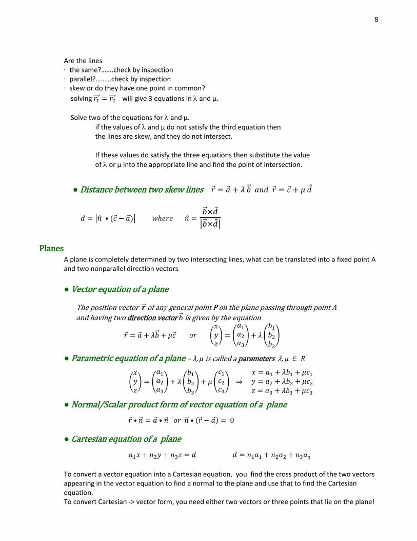
Are the lines ∙ the same?…….check by inspection

∙ parallel?………check by inspection

∙ skew or do they have one point in common?

solving 𝑟1⃗⃗⃗ ⃗ = 𝑟2⃗⃗⃗⃗ will give 3 equations in and µ.

Solve two of the equations for and µ.

if the values of and µ do not satisfy the third equation then the lines are skew, and they do not intersect.

If these values do satisfy the three equations then substitute the value

of or µ into the appropriate line and find the point of intersection.

● Distance between two skew lines 𝑟 = �⃗� + 𝜆 �⃗⃗� 𝑎𝑛𝑑 𝑟 = 𝑐 + 𝜇 𝑑

𝑑 = |�̂� • (𝑐 − �⃗�)| 𝑤ℎ𝑒𝑟𝑒 �̂� = �⃗⃗�×�⃗�

|�⃗⃗�×�⃗�|

Planes

A plane is completely determined by two intersecting lines, what can be translated into a fixed point A and two nonparallel direction vectors

● Vector equation of a plane

The position vector �⃗⃗� of any general point P on the plane passing through point A

and having two direction vector �⃗⃗� is given by the equation

𝑟 = �⃗� + 𝜆�⃗⃗� + 𝜇𝑐 𝑜𝑟 (𝑥𝑦𝑧) = (

𝑎1𝑎2𝑎3) + 𝜆(

𝑏1𝑏2𝑏3

)

● Parametric equation of a plane – λ, 𝜇 is called a parameters λ, 𝜇 ∈ 𝑅

(𝑥𝑦𝑧) = (

𝑎1𝑎2𝑎3) + 𝜆(

𝑏1𝑏2𝑏3

) + 𝜇 (

𝑐1𝑐2𝑐3) ⇒

𝑥 = 𝑎1 + 𝜆𝑏1 + 𝜇𝑐1𝑦 = 𝑎2 + 𝜆𝑏2 + 𝜇𝑐2𝑧 = 𝑎3 + 𝜆𝑏3 + 𝜇𝑐3

● Normal/Scalar product form of vector equation of a plane

𝑟 • �⃗⃗� = �⃗� • �⃗⃗� 𝑜𝑟 �⃗⃗� • (𝑟 − �⃗�) = 0

● Cartesian equation of a plane

𝑛1𝑥 + 𝑛2𝑦 + 𝑛3𝑧 = 𝑑 𝑑 = 𝑛1𝑎1 + 𝑛2𝑎2 + 𝑛3𝑎3

To convert a vector equation into a Cartesian equation, you find the cross product of the two vectors appearing in the vector equation to find a normal to the plane and use that to find the Cartesian equation. To convert Cartesian -> vector form, you need either two vectors or three points that lie on the plane!

9

𝑥 + 3𝑦 − 2𝑧 = 5 3𝑥 + 5𝑦 + 6𝑧 = 7 2𝑥 + 4𝑦 + 3𝑧 = 8

So first step is to choose three arbitrary random non-collinear points.

● Distance from origin

𝐷 = |𝑟 • �̂�| = |�⃗� • �̂�| = |𝑛1𝑎1+𝑛2𝑎2+𝑛3𝑎3 |

√𝑛12+𝑛2

2+𝑛32

● Intersection of a line and a plane

𝐿𝑖𝑛𝑒 𝐿: 𝑟 = (1−2−1) + 𝜇 (

456) 𝑎𝑛𝑑 𝑝𝑙𝑎𝑛𝑒 𝛱: 𝑥 + 2𝑦 + 3𝑧 = 5

To check if the line is parallel to the plane do dot product of direction vector of the line and normal vector to the plane. If dot product is not zero the line and the plane are not parallel and the line will intersect the plane in one point.

Substitute the line equation into the plane equation to obtain the value of the line parameter µ.

(1 + 4𝜇) + 2(−2 + 5𝜇) + 3(−1 + 6𝜇) = 5 1 + 4µ − 4 + 10µ − 3 + 18µ = 5 ⇒ 𝜇 =11

32

Substitute µ into the equation of the line to obtain the co-ordinates of the point of intersection:

1

32(76−934)

In general: Solve for µ and substitute into the equation of the line to get the point of intersection. If this equation gives you something like 0 = 5, then the line will be parallel and not in the plane, and if the equation gives you something like 5 = 5 then the line is contained in the plane.

System of Linear Equations

Consider the following linear system :

THE A LINEAR SYSTEM MAY BEHAVE IN ANY OF THREE POSSIBLE WAYS 1. The system has a single unique solution. 2. The system has no solution. 3. The system has infinitely many solutions. For three variables, each linear equation is a plane in 3-D space, and the solution set is the intersection of these planes. Thus the solution set may be a plane, a line, a single point, or the empty set.

~ [1 3 −23 5 62 4 3

|578]

The augmented matrix

10

Example: solution is a single point: Combine two at the time to eliminate one variable

1. step:

(1. 𝑒𝑞𝑢𝑎𝑡𝑖𝑜𝑛) ∙ (−3) + (2. 𝑒𝑞𝑢𝑎𝑡𝑖𝑜𝑛) = 𝑛𝑒𝑤 𝑠𝑒𝑐𝑜𝑛𝑑 𝑒𝑞𝑢𝑎𝑡𝑖𝑜𝑛 (𝑛𝑜 𝑥 𝑎𝑛𝑦 𝑚𝑜𝑟𝑒)

(1. 𝑒𝑞𝑢𝑎𝑡𝑖𝑜𝑛) ∙ (−2) + (3. 𝑒𝑞𝑢𝑎𝑡𝑖𝑜𝑛) = 𝑛𝑒𝑤 𝑡ℎ𝑖𝑟𝑑 𝑒𝑞𝑢𝑎𝑡𝑖𝑜𝑛 (𝑛𝑜 𝑥 𝑎𝑛𝑦 𝑚𝑜𝑟𝑒)

2. step

(2. 𝑒𝑞𝑢𝑎𝑡𝑖𝑜𝑛) ∙ (−1

2) + (3. 𝑒𝑞𝑢𝑎𝑡𝑖𝑜𝑛) = 𝑛𝑒𝑤 𝑡ℎ𝑖𝑟𝑑 𝑒𝑞𝑢𝑎𝑡𝑖𝑜𝑛 (𝑛𝑜 𝑦 𝑎𝑛𝑦 𝑚𝑜𝑟𝑒)

−2𝑥 − 6𝑦 + 4𝑧 = −10−3𝑥 − 9𝑦 + 6𝑧 = −15

2𝑦 − 6𝑧 = 4

𝑥 + 3𝑦 − 2𝑧 = 5 3𝑥 + 5𝑦 + 6𝑧 = 7 2𝑥 + 4𝑦 + 3𝑧 = 8

~ 𝑥 + 3𝑦 − 2𝑧 = 5 −4𝑦 + 12𝑧 = −8 −2𝑦 + 7𝑧 = −2

~ 𝑥 + 3𝑦 − 2𝑧 = 5 −4𝑦 + 12𝑧 = −8 𝑧 = 2

This is equivalent to say that augmented matrix is in reduced row echelon form – augmented matrix with the zeroes in the bottom left corner.

[1 3 −23 5 62 4 3

|578] ~ [

1 3 −20 −4 120 −2 7

|5−8−2] ~ [

1 3 −20 −4 120 0 1

|5−82] ~

𝑥 + 3𝑦 − 2𝑧 = 5 −4𝑦 + 12𝑧 = −8 𝑧 = 2

solution::

𝒛 = 𝟐 𝐲 = 𝟖 𝒙 = −𝟏𝟓

Generally, using this method we get augmented matrix of coefficients of the system in echelon form

Echelon form

[𝑎 𝑏 𝑐0 𝑒 𝑓0 0 ℎ

|𝑑𝑔𝑘] ~

𝑎𝑥 + 𝑏𝑦 + 𝑐𝑧 = 𝑑 𝑒𝑦 + 𝑓𝑧 = 𝑔 ℎ𝑧 = 𝑘

→ 𝑧 =𝑘

ℎ → 𝑦 & 𝑥

𝒖𝒏𝒊𝒒𝒖𝒆 𝒔𝒐𝒍𝒖𝒕𝒊𝒐𝒏: ℎ ≠ 0 → 𝑧 =

𝑘

ℎ → 𝑦 & 𝑥 (𝑘 𝑚𝑎𝑦 𝑜𝑟 𝑚𝑎𝑦 𝑛𝑜𝑡 𝑏𝑒 0)

𝒏𝒐 𝒔𝒐𝒍𝒖𝒕𝒊𝒐𝒏: ℎ = 0 𝑎𝑛𝑑 𝑘 ≠ 0 → 0 ∙ 𝑧 = 𝑘 ≠ 0 𝑤ℎ𝑖𝑐ℎ 𝑖𝑠 𝑎𝑏𝑠𝑢𝑟𝑑 →

𝑡ℎ𝑒𝑟𝑒 𝑖𝑠 𝑛𝑜 𝑠𝑜𝑙𝑢𝑡𝑖𝑜𝑛 (𝑠𝑦𝑠𝑡𝑒𝑚 𝑖𝑠 𝒊𝒏𝒄𝒐𝒏𝒔𝒊𝒔𝒕𝒆𝒏𝒕)

𝒊𝒏𝒇𝒊𝒏𝒊𝒕𝒆𝒍𝒚 𝒎𝒂𝒏𝒚 𝒔𝒐𝒍𝒖𝒕𝒊𝒐𝒏𝒔: ℎ = 0 𝑎𝑛𝑑 𝑘 = 0 → 𝑧 𝑐𝑎𝑛 𝑏𝑒 𝑎𝑛𝑦 𝑛𝑢𝑚𝑏𝑒𝑟, 𝑠𝑜 𝑤𝑒 𝑤𝑟𝑖𝑡𝑒:

𝑧 = 𝑡 𝑤ℎ𝑒𝑟𝑒 𝑡 ∈ 𝑅

𝑥 = 𝑥(𝑡)

𝑦 = 𝑦(𝑡)

𝑧 = 𝑡

Parametric representation of infinitely many solutions is not unique. We expressed the variable which was not free (z) in terms of the parameter. We eliminated from row 3 variables x and y. It does not have to be that way. We could eliminate z and y to get x, and then express y and z. One can solve for any of the variables. Of course, the solution set will look different. However, it will still represent the same solutions.

11

Example:

𝑢𝑛𝑖𝑞𝑢𝑒 𝑠𝑜𝑙𝑢𝑡𝑖𝑜𝑛: [1 1 10 2 20 0 3

|126] → 𝑧 = 2 𝑦 = −1 𝑥 = 0 𝑃(0, −1,2)

𝑛𝑜 𝑠𝑜𝑙𝑢𝑡𝑖𝑜𝑛: [1 1 10 2 20 0 0

|123] → 𝑧 ∙ 0 = 3 𝑎𝑏𝑠𝑢𝑟𝑑

𝑖𝑛𝑓𝑖𝑛𝑒𝑡𝑒𝑙𝑦 𝑚𝑎𝑛𝑦 𝑠𝑜𝑙𝑢𝑡𝑖𝑜𝑛𝑠: [1 1 10 2 20 0 0

|120] → 𝑧 ∙ 0 = 0 ⏟

𝑡𝑟𝑢𝑒 𝑓𝑜𝑟 𝑎𝑛𝑦 𝑧

⇒ 𝑧 = 𝑡 𝜖 𝑅 𝑦 = 1 − 𝑡 𝑥 = 0

Counting principles, including permutations and combinations.

The binomial theorem: expansion of (𝒂 + 𝒃)𝒏, 𝒏 𝜺 𝑵.

If there are 𝑚 different ways of performing an operation and for each of these there are 𝑛 different ways of performing a second independent operation, then there are 𝑚𝑛 different ways of performing the two operations in succession. The product principle can be extended to three or more successive operations. The number of different ways of performing an operation is equal to the sum of the different mutually exclusive possibilities.

The word 𝑎𝑛𝑑 suggests multiplying the possibilities

The word 𝑜𝑟 suggests adding the possibilities.

If the order doesn't matter, it is a Combination.

If the order does matter it is a Permutation.

A permutation of a group of symbols is any arrangement of those symbols in a definite order.

Explanation: Assume you have n different symbols and therefore n places to fill in your arrangement. For the first place, there are n different possibilities. For the second place, no matter what was put in the first place, there are n – 1 possible symbols to place, for the rth place there are n – r +1 possible places until the point where r = n, at which point we have saturated all the places. According to the product principle, therefore, we have n (n – 1)(n – 2)(n – 3)⋯1 different arrangements, or n!

● THE PRODUCT RULE

● COUNTING PATHS

● PERMUTATIONS (order matters)

● Permutations of 𝒏 different object : 𝒏!

12

Wise Advice: If a group of items have to be kept together, treat the items as one object. Remember that there may be permutations of the items within this group too.

Suppose we have 10 letters and want to make groups of 4 letters. For four-letter permutations, there are 10 possibilities for the first letter, 9 for the second, 8 for the third, and 7 for the last letter. We can find the total number of different four-letter permutations by multiplying 10 x 9 x 8 x 7 = 5040. Good logic to apply to similar questions straightforward!!!

There are n possibilities for the first choice, THEN there are n possibilities for the second choice, and so on, multiplying each time.)

It is the number of ways of choosing 𝒌 objects out of 𝒏 available given that ▪ The order of the elements does not matter. ▪ The elements are not repeated [such as lottery numbers (2,14,15,27,30,33)]

The easiest way to explain it is to: assume that the order does matter (ie permutations), then alter it so the order does not matter.

Since the combination does not take into account the order, we have to divide the permutation of the total number of symbols available by the number of redundant possibilities. 𝒌 selected objects have a number of redundancies equal to the permutation of the objects 𝒌! (since order doesn’t matter) However, we also need to divide the permutation n! by the permutation of the objects that are not selected, that is to say (𝒏 − 𝒌)! .

𝒏!

𝒌! (𝒏 − 𝒌)!

(𝒏𝒌) ≡ 𝑪𝒌

𝒏 ≡ 𝑪𝒌𝒏 =

𝒏!

𝒌! (𝒏 − 𝒌)!=𝒏(𝒏 − 𝟏)(𝒏 − 𝟐)(𝒏 − 𝒌 + 𝟏)

𝒌!

● Binomial Expansion/Theorem

(𝑎 + 𝑏)𝑛 = ∑(𝑛𝑘) 𝑎𝑛−𝑘𝑏𝑘 = 𝑎𝑛 + (

𝑛1) 𝑎𝑛−1𝑏 +⋯+ (

𝑛𝑘) 𝑎𝑛−𝑘𝑏𝑘 +⋯+ 𝑏𝑛

𝑛

𝑘=0

● Permutations of 𝒌 different objects out of 𝒏 different available : 𝒏 ∙ (𝒏 − 𝟏) ∙∙∙ (𝒏 − 𝒌 + 𝟏)

● Permutations with repetition of 𝒌 different objects out of 𝒏 different available = 𝒏𝒌

● COMBINATIONS (order doesn’t matters)

𝑛 𝜀 𝑁 (𝑛0) ≡ 1 0! ≡ 1

13

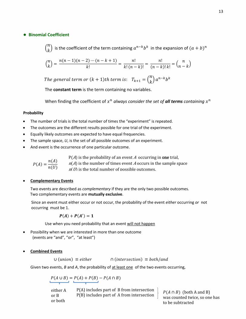
● Binomial Coefficient

(𝑛𝑘) is the coefficient of the term containing 𝑎𝑛−𝑘𝑏𝑘 in the expansion of (𝑎 + 𝑏)𝑛

(𝑛𝑘) =

𝑛(𝑛 − 1)(𝑛 − 2)⋯ (𝑛 − 𝑘 + 1)

𝑘!=

𝑛!

𝑘! (𝑛 − 𝑘)!=

𝑛!

(𝑛 − 𝑘)! 𝑘!= (

𝑛𝑛 − 𝑘

)

𝑇ℎ𝑒 𝑔𝑒𝑛𝑒𝑟𝑎𝑙 𝑡𝑒𝑟𝑚 𝑜𝑟 (𝑘 + 1)𝑡ℎ 𝑡𝑒𝑟𝑚 𝑖𝑠: 𝑇𝑘+1 = (𝑛𝑘) 𝑎𝑛−𝑘𝑏𝑘

The constant term is the term containing no variables. When finding the coefficient of 𝑥𝑛 always consider the set of all terms containing 𝑥𝑛

Probability

The number of trials is the total number of times the “experiment” is repeated.

The outcomes are the different results possible for one trial of the experiment.

Equally likely outcomes are expected to have equal frequencies.

The sample space, U, is the set of all possible outcomes of an experiment.

And event is the occurrence of one particular outcome.

𝑃(𝐴) =𝑛(𝐴)

𝑛(𝑈)

Complementary Events

Two events are described as complementary if they are the only two possible outcomes. Two complementary events are mutually exclusive.

Since an event must either occur or not occur, the probability of the event either occurring or not occurring must be 1.

𝑷(𝑨) + 𝑷(𝑨′) = 𝟏

Use when you need probability that an event will not happen

Possibility when we are interested in more than one outcome (events are “and”, “or”, “at least”)

Combined Events

∪ (𝑢𝑛𝑖𝑜𝑛) ≡ 𝑒𝑖𝑡ℎ𝑒𝑟 ∩ (𝑖𝑛𝑡𝑒𝑟𝑠𝑒𝑐𝑡𝑖𝑜𝑛) ≡ 𝑏𝑜𝑡ℎ/𝑎𝑛𝑑

Given two events, B and A, the probability of at least one of the two events occurring,

𝑃(𝐴 ∪ 𝐵) = 𝑃(𝐴) + 𝑃(𝐵) − 𝑃(𝐴 ∩ 𝐵)

P(A) is the probability of an event A occurring in one trial,

n(A) is the number of times event A occurs in the sample space

n(U) is the total number of possible outcomes.

either A or B or both

P(A) includes part of B from intersection P(B) includes part of A from intersection

𝑃(𝐴 ∩ 𝐵) (both A and B) was counted twice, so one has to be subtracted

14

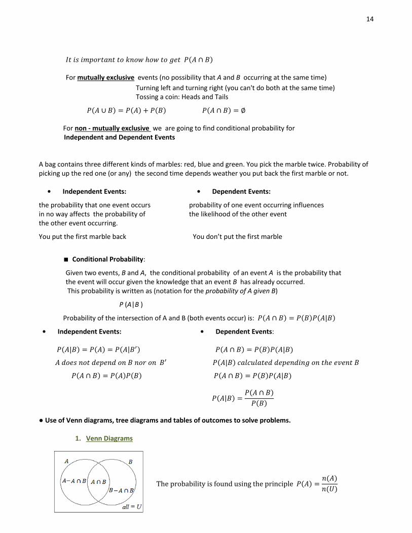
𝐼𝑡 𝑖𝑠 𝑖𝑚𝑝𝑜𝑟𝑡𝑎𝑛𝑡 𝑡𝑜 𝑘𝑛𝑜𝑤 ℎ𝑜𝑤 𝑡𝑜 𝑔𝑒𝑡 𝑃(𝐴 ∩ 𝐵)

For mutually exclusive events (no possibility that A and B occurring at the same time)

Turning left and turning right (you can't do both at the same time) Tossing a coin: Heads and Tails

𝑃(𝐴 ∪ 𝐵) = 𝑃(𝐴) + 𝑃(𝐵) 𝑃(𝐴 ∩ 𝐵) = ∅ For non - mutually exclusive we are going to find conditional probability for

Independent and Dependent Events

A bag contains three different kinds of marbles: red, blue and green. You pick the marble twice. Probability of picking up the red one (or any) the second time depends weather you put back the first marble or not. • Independent Events: • Dependent Events:

the probability that one event occurs probability of one event occurring influences in no way affects the probability of the likelihood of the other event the other event occurring.

You put the first marble back You don’t put the first marble

∎ Conditional Probability:

Given two events, B and A, the conditional probability of an event A is the probability that the event will occur given the knowledge that an event B has already occurred. This probability is written as (notation for the probability of A given B)

P (A|B )

Probability of the intersection of A and B (both events occur) is: 𝑃(𝐴 ∩ 𝐵) = 𝑃(𝐵)𝑃(𝐴|𝐵)

• Independent Events: • Dependent Events: 𝑃(𝐴|𝐵) = 𝑃(𝐴) = 𝑃(𝐴|𝐵′) 𝑃(𝐴 ∩ 𝐵) = 𝑃(𝐵)𝑃(𝐴|𝐵)

𝐴 𝑑𝑜𝑒𝑠 𝑛𝑜𝑡 𝑑𝑒𝑝𝑒𝑛𝑑 𝑜𝑛 𝐵 𝑛𝑜𝑟 𝑜𝑛 𝐵′ 𝑃(𝐴|𝐵) 𝑐𝑎𝑙𝑐𝑢𝑙𝑎𝑡𝑒𝑑 𝑑𝑒𝑝𝑒𝑛𝑑𝑖𝑛𝑔 𝑜𝑛 𝑡ℎ𝑒 𝑒𝑣𝑒𝑛𝑡 𝐵

𝑃(𝐴 ∩ 𝐵) = 𝑃(𝐴)𝑃(𝐵) 𝑃(𝐴 ∩ 𝐵) = 𝑃(𝐵)𝑃(𝐴|𝐵)

𝑃(𝐴|𝐵) =𝑃(𝐴 ∩ 𝐵)

𝑃(𝐵)

● Use of Venn diagrams, tree diagrams and tables of outcomes to solve problems.

1. Venn Diagrams

The probability is found using the principle 𝑃(𝐴) =𝑛(𝐴)

𝑛(𝑈)

15

2. Tree diagrams

A more flexible method for finding probabilities is known as a tree diagram.

This allows one to calculate the probabilities of the occurrence of events, even where trials are non-identical (where 𝑃(𝐴|𝐴) ≠ 𝑃(𝐴)), through the product principle.

⧪ Bayes’ Theorem

𝑃(𝐴 ∩ 𝐵) = 𝑃(𝐵)𝑃(𝐴|𝐵) ⟹ 𝑃(𝐴 ∩ 𝐵) = 𝑃(𝐴)𝑃(𝐵|𝐴)

𝑃(𝐴|𝐵) = 𝑃(𝐴 ∩ 𝐵)

𝑃(𝐵)=𝑃(𝐴)𝑃(𝐵|𝐴)

𝑃(𝐵) 𝐵𝑎𝑦𝑒𝑠′ 𝑡ℎ𝑒𝑜𝑟𝑒𝑚

▪ Another form of Bayes’ theorem (Formula booklet)

From tree diagram: there are two ways to get A, either after B has happen or after B has not happened:

16

𝑃(𝐴) = 𝑃(𝐵)𝑃(𝐴|𝐵) + 𝑃(𝐵′)𝑃(𝐴|𝐵′) ⟹ 𝑃(𝐵|𝐴) =𝑃(𝐵)𝑃(𝐴|𝐵)

𝑃(𝐵)𝑃(𝐴|𝐵) + 𝑃(𝐵′)𝑃(𝐴|𝐵′)

▪ Extension of Bayes’ Theorem

If there are more options than simply B occurs or B doesn’t occur, for example if there were three possible outcomes for the first event B1, B2, and B3

Probability of A occurring is: 𝑃(𝐵1)𝑃(𝐴|𝐵1) + 𝑃(𝐵2)𝑃(𝐴|𝐵2) + 𝑃(𝐵3)𝑃(𝐴|𝐵3)

𝑃(𝐵𝑖|𝐴) =𝑃(𝐵𝑖)𝑃(𝐴|𝐵𝑖)

𝑃(𝐵1)𝑃(𝐴|𝐵1) + 𝑃(𝐵2)𝑃(𝐴|𝐵2) + 𝑃(𝐵3)𝑃(𝐴|𝐵3)

Outcomes B1, B2, and B3 must cover all the possible outcomes.

Descriptive Statistics

Concepts of population, sample, random sample and frequency distribution of discrete and continuous data.

A population is the set of all individuals with a given value for a variable associated with them.

A sample is a small group of individuals randomly selected (in the case of a random sample) from the population as a whole, used as a representation of the population as a whole.

The frequency distribution of data is the number of individuals within a sample or population for each value of the associated variable in discrete data, or for each range of values for the associated variable in continuous data.

Presentation of data: frequency tables and diagrams

Grouped data: mid-interval values, interval width, upper and lower interval boundaries, frequency histograms.

17

Mid interval values are found by halving the difference between the upper and lower interval boundaries.

The interval width is simply the distance between the upper and lower interval boundaries.

Frequency histograms are drawn with interval width proportional to bar width and frequency as the height.

Median, mode; quartiles, percentiles.

Range; interquartile range; variance, standard deviation.

Mode (discrete data) is the most frequently occurring value in the data set.

Modal class (continuous data) is the most frequently occurring class.

Median is the middle value of an ordered data set.

For an odd number of data, the median is middle data.

For an even number of data, the median is average of two middle data.

Percentile is the score bellow which a certain percentage of the data lies.

Lower quartile (Q1) is the 25th percentile.

Median (Q2) is the 50th percentile.

Upper quartile (Q3) is the 75th percentile.

Range is the difference between the highest and lowest value in the data set.

The interquartile range is Q3−Q1.

Cumulative frequency is the frequency of all values less than a given value.

The population mean, μ is generally unknown but the sample mean, �̅� used to serve as an unbiased estimate of this mean. That used to be. From now on for the examination purposes, data will be treated as the population. Estimation of mean and variance of population from a sample is no longer required.

A variable X whose value depends on the outcome of a random process is called a random variable. For any random variable there is a probability distribution/ function associated with it.

● Probability distribution/ function

Discrete Random Variables

P(X = x), the probability distribution of x, involves listing P(𝑥𝑖 ) for each 𝑥𝑖. 1. 0 ≤ 𝑃(𝑋 = 𝑥) ≤ 1

2. ∑𝑃(𝑋 = 𝑥) = 1

𝑥

3. 𝑃(𝑋 = 𝑥𝑛)

= 1 −∑ 𝑃(𝑋 = 𝑥𝑘)

𝑘≠𝑛

[𝑃 (𝑒𝑣𝑒𝑛𝑡 𝑥𝑛 𝑜𝑐𝑐𝑢𝑟𝑠) = 1 − 𝑃(𝑎𝑛𝑦 𝑜𝑡ℎ𝑒𝑟 𝑒𝑣𝑒𝑛𝑡 𝑜𝑐𝑐𝑢𝑟𝑠)]

Discrete and Continuous Random Variables

18

Discrete Random Variables X defined on a ≤ x ≤ b

probability density function (p.d.f.), f (x), describes the relative likelihood for this variable to take on a given value cumulative distribution function ( c.d.f.), 𝐹(𝑡), is found by integrating the p.d.f. between the minimum value of X and t

𝐹(𝑡) = 𝑃(𝑋 ≤ 𝑡) = ∫𝑓(𝑥)𝑑𝑥

𝑡

𝑎

1. 𝑓(𝑥) ≥ 0 𝑓𝑜𝑟 𝑎𝑙𝑙 𝑥 𝜖 (𝑎, 𝑏)

2. ∫ 𝑓(𝑥) = 1

𝑏

𝑎

3. 𝑓𝑜𝑟 𝑎𝑛𝑦 𝑎 ≤ 𝑐 < 𝑑 ≤ 𝑏, 𝑃(𝑐 < 𝑋 < 𝑑) = ∫ 𝑓(𝑥)𝑑𝑥

𝑑

𝑐

▪ 𝐹𝑜𝑟 𝑎 𝑐𝑜𝑛𝑡𝑖𝑛𝑢𝑜𝑢𝑠 𝑟𝑎𝑛𝑑𝑜𝑚 𝑣𝑎𝑟𝑖𝑎𝑏𝑙𝑒, 𝑡ℎ𝑒 𝑝𝑟𝑜𝑏𝑎𝑏𝑖𝑙𝑖𝑡𝑦 𝑜𝑓 𝑎𝑛𝑦 𝑠𝑖𝑛𝑔𝑙𝑒 𝑣𝑎𝑙𝑢𝑒 𝑖𝑠 𝑧𝑒𝑟𝑜

𝑃(𝑋 = 𝑐) = 0 ⇒ 𝑃(𝑐 ≤ 𝑋 ≤ 𝑑) = 𝑃(𝑐 < 𝑋 < 𝑑) = 𝑃(𝑐 ≤ 𝑋 < 𝑑) 𝑒𝑡𝑐.

Expected value (or mean) is a weighted average of the possible values that X can take, each value

being weighted according to the probability of that event occurring.

Discrete Random Variables Continuous Random Variables

𝑬(𝑿) = 𝝁 = ∑𝒙 𝑷(𝑿 = 𝒙) 𝑬(𝑿) = 𝝁 = ∫ 𝒙 𝒇(𝒙)𝒅𝒙

∞

−∞

Properties of expected value 𝑬(𝑿)

1. 𝐼𝑓 𝑎 𝑎𝑛𝑑 𝑏 𝑎𝑟𝑒 𝑐𝑜𝑛𝑠𝑡𝑎𝑛𝑡𝑠, 𝑡ℎ𝑒𝑛 𝐸(𝑎𝑋 + 𝑏) = 𝑎𝐸(𝑋) + 𝑏 2. 𝐸(𝑋 + 𝑌 ) = 𝐸(𝑋) + 𝐸(𝑌 )

Expected Value of a Function of X

𝐸[ 𝑔(𝑋)], 𝑤ℎ𝑒𝑟𝑒 𝑔(𝑋) 𝑖𝑠 𝑎 𝑓𝑢𝑛𝑐𝑡𝑖𝑜𝑛 𝑜𝑓 𝑋 𝑖𝑠:

Discrete Random Variables Continuous Random Variables

𝐸[ 𝑔(𝑋)] = ∑𝑔(𝑥)𝑃(𝑋 = 𝑥) 𝐸[ 𝑔(𝑋)] = ∫ 𝑔(𝑥)𝑓(𝑥)𝑑𝑥

sum of: [(each of the possible outcomes)

× (the probability of the outcome occurring)].

19

Mode is the most likely value of X.

Discrete Random Variables

The mode is the value of x with largest 𝑃(𝑋 = 𝑥) which can be different from the expected value

Continuous Random Variables The mode is the value of x where f(x) is maximum (which may not be unique).

Median

Discrete Random Variables

The median of a discrete random variable is the "middle" value. It is the value of X such that

𝑃(𝑋 ≤ 𝑥) ≥1

2 𝑎𝑛𝑑 𝑃(𝑋 ≥ 𝑥) ≥

1

2

Continuous Random Variables

The median of a random variable X is a number m such that

∫ 𝑓(𝑥) =1

2

𝑚

𝑎

The median m is the number for which the probability is exactly ½ that the random variable will have a value greater than m, and ½ that it will have a value less than m.

Variance

The variance of a random variable tells us something about the spread of the possible values of the

variable. Variance, Var( X ), is defined as the average of the squared differences of X from the mean:

𝑽𝒂𝒓(𝑿) = 𝝈𝟐 = 𝑬 (𝑿 – 𝝁)𝟐 = 𝑬(𝑿𝟐) − 𝝁𝟐

Discrete Random Variables

𝑽𝒂𝒓(𝑿) = 𝛴𝑥2 𝑃(𝑋 = 𝑥) − 𝜇2

Continuous Random Variables

𝑽𝒂𝒓(𝑿) = ∫𝑥2𝑓(𝑥)𝑑𝑥 − 𝜇2

𝑏

𝑎

Properties of variance

Note that the variance does not behave in the same way as expectation when we multiply and add constants to random variables. In fact:

20

𝑉 𝑎𝑟(𝑎𝑋 + 𝑏) = 𝑎2𝑉𝑎𝑟(𝑋)

𝐼𝑛 𝑔𝑒𝑛𝑒𝑟𝑎𝑙 𝑉𝑎𝑟[𝑋 + 𝑌] ≠ 𝑉𝑎𝑟(𝑋) + 𝑉𝑎𝑟(𝑌) (only for independent − not IB)

Standard deviation of X

𝜎 = √𝑉𝑎𝑟(𝑋)

Binomial Distribution - Discrete There are three criteria that must be met in order for a random probability distribution to be a binomial

distribution.

The experiment consists of n repeated trials.

Each trial can result in just two possible outcomes. We call one of these outcomes a success and

the other, a failure.

The probability of success, denoted by p, is the same on every trial.

The trials are independent; that is, the outcome on one trial does not affect the outcome on other

trials – the probability of success is a constant in each trial

If a random variable X has a binomial distribution, we write

• 𝑿 ~ 𝑩(𝒏, 𝒑) (~ means ‘has distribution…’).

and the probability density function is:

• 𝑃(𝑋 = 𝑥) = (𝑛𝑥)𝑝𝑥(1 − 𝑝)𝑛−𝑥 𝑥 = 0, 1, … , 𝑛

• n is number of trials

• p is the probability of a success

• (1 – p) is the probability of a failure.

If X is a random variable is binomial with parameters n and p, then mean and variance are: •

𝐸(𝑋) = 𝜇 = 𝑛𝑝

• 𝑉𝑎𝑟(𝑋) = 𝜎2 = 𝑛𝑝(1 − 𝑝)

21

Poisson Distribution

A discrete random variable X with a probability distribution function (p.d.f.) of the form:

• 𝑃(𝑋 = 𝑥) =𝑚𝑥𝑒−𝑚

𝑥!, 𝑥 = 0, 1, 2, …

is said to be a Poisson random variable with parameter m. We write • 𝑋 ~ 𝑃𝑜(𝑚)

Mean and Variance

𝐼𝑓 𝑋 ~ 𝑃𝑜(𝑚), 𝑡ℎ𝑒𝑛 • 𝐸(𝑋) = 𝑚

• 𝑉𝑎𝑟(𝑋) = 𝑚 Random Events The Poisson distribution is useful because many random events follow it. If a random event has a mean number of occurrences m in a given time period, then the number of occurrences within that time period will follow a Poisson distribution. For example, the occurrence of earthquakes could be considered to be a random event. If there are 5 major earthquakes each year, then the number of earthquakes in any given year will have a Poisson distribution with parameter 5.

There are three criteria that must be met in order for a random probability distribution to be a

Poisson distribution.

The average number of occurrences (m) is constant for every interval.

The probability of more than one occurrence in a given interval is very small.

The number of occurrences in disjoint intervals are independent of each other.

Sums of Poissons

Suppose X and Y are independent Poisson random variables with parameters ℓ and m respectively. Then X + Y has a Poisson distribution with parameter ℓ + m. In other words: If 𝑿 ~ 𝑷𝒐(𝓵), and 𝒀 ~ 𝑷𝒐(𝒎), ), then 𝑿 + 𝒀~ 𝑷𝒐(𝓵 +𝒎)

22

Normal distribution. Standardization of normal variables.

A continuous random variable X follows a normal distribution if it has the following probability density function :

• 𝑓(𝑥) =1

𝜎√2𝜋 𝑒−12(𝑥−𝜇𝜎)2

− ∞ < 𝑥 < ∞

The parameters of the distribution are μ and 𝝈𝟐, where μ is the mean (expectation) of the distribution and 𝜎2 is the variance.

𝑿 ~ 𝑵(𝝁, 𝝈𝟐) the random variable X has a normal distribution with parameters μ and 𝜎2.

Properties

1. 𝑑𝑓

𝑑𝑥 𝑓(𝑥) = −

1

𝜎2√2𝜋(𝑥 − 𝜇

𝜎) 𝑒

−12(𝑥−𝜇𝜎)2

= 0 ⇒ 𝑚𝑎𝑥𝑖𝑚𝑢𝑚 : 𝒙 = 𝝁

2. 𝑑𝑓

𝑑𝑥 𝑓(𝑥) = −

1

𝜎3√2𝜋[1 − (

𝑥 − 𝜇

𝜎)2

] 𝑒−12(𝑥−𝜇𝜎)2

= 0 ⇒ 𝑖𝑛𝑓𝑙𝑒𝑐𝑡𝑖𝑜𝑛𝑠: 𝒙 = 𝝁 ± 𝝈

The curve is symmetrical about the line x = μ

▪ lim𝑥→±∞

𝑓(𝑥) = 0

▪ ∫ 𝑓(𝑥)

∞

−∞

= 1

▪ 𝜇 = 𝑚𝑎𝑥{𝑓(𝑥)}

For a normal curve, standard deviation σ is uniquely determined as the horizontal distance from the

vertical line of symmetry 𝑥 = 𝜇 to the point of inflection.

In a normal distribution, 68.26% of values lie within one standard deviation of the mean, 95.4% of values lie within two standard deviations of the mean and 99.74% of values lie within three standard deviations of the mean.

Standard score or z – score is the number of standard deviations from the mean.

The Standard Normal Distribution

If 𝑍 ~ 𝑁(0, 1), then Z is said to follow a standard normal distribution. P(Z < z) is known as the cumulative distribution function of the random variable Z. For the standard normal distribution, this is usually denoted by F(z). Normally, you would work out the c.d.f. by doing some integration. However, it is impossible to do this for the normal distribution and so results have to be looked up in statistical tables.

23

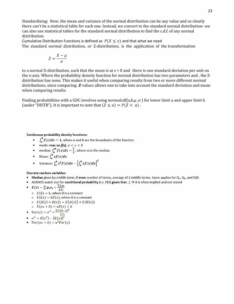
Standardising: Now, the mean and variance of the normal distribution can be any value and so clearly there can't be a statistical table for each one. Instead, we convert to the standard normal distribution- we can also use statistical tables for the standard normal distribution to find the c.d.f. of any normal distribution. Cumulative Distribution Functions is defined as 𝑃(𝑋 ≤ 𝑥) and that what we need The standard normal distribution, or Z-distribution, is the application of the transformation

𝑍 =𝑋 − 𝜇

𝜎

to a normal X-distribution, such that the mean is at x = 0 and there is one standard deviation per unit on the x-axis. Where the probability density function for normal distribution has two parameters and , the Z-distribution has none. This makes it useful when comparing results from two or more different normal distributions, since comparing Z-values allows one to take into account the standard deviation and mean when comparing results. Finding probabilities with a GDC involves using normalcdf(a,b,μ ,σ ) for lower limit a and upper limit b (under “DISTR”). It is important to note that (𝑍 ≤ 𝑎) = 𝑃(𝑍 < 𝑎) .

24

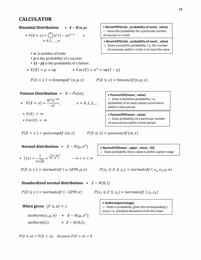
CALCULATOR

Binomial Distribution • 𝑿 ~ 𝑩(𝒏, 𝒑)

• 𝑃(𝑋 = 𝑥) = (𝑛𝑥)𝑝𝑥(1 − 𝑝)𝑛−𝑥 𝑥

= 0, 1, … , 𝑛

• n is number of trials

• p is the probability of a success

• (1 – p) is the probability of a failure.

• 𝐸(𝑋) = 𝜇 = 𝑛𝑝 • 𝑉𝑎𝑟(𝑋) = 𝜎2 = 𝑛𝑝(1 − 𝑝)

𝑃(𝑋 = 𝑥 ) = 𝑏𝑖𝑛𝑜𝑚𝑝𝑑𝑓 (𝑛, 𝑝, 𝑥) 𝑃(𝑋 ≤ 𝑥) = 𝑏𝑖𝑛𝑜𝑚𝑐𝑑𝑓(𝑛, 𝑝, 𝑥)

Poisson Distribution • 𝑋 ~ 𝑃𝑜(𝑚)

• 𝑃(𝑋 = 𝑥) =𝑚𝑥𝑒−𝑚

𝑥!, 𝑥 = 0, 1, 2, …

• 𝐸(𝑋) = 𝑚

• 𝑉𝑎𝑟(𝑋) = 𝑚 𝑃(𝑋 = 𝑥 ) = 𝑝𝑜𝑖𝑠𝑠𝑜𝑛𝑝𝑑𝑓 (𝑚, 𝑥) 𝑃(𝑋 ≤ 𝑥) = 𝑝𝑜𝑖𝑠𝑠𝑜𝑛𝑐𝑑𝑓(𝑚, 𝑥)

Normal distribution. • 𝑋 ~ 𝑁(𝜇, 𝜎2)

• 𝑓(𝑥) =1

𝜎√2𝜋 𝑒−12(𝑥−𝜇𝜎)2

− ∞ < 𝑥 < ∞

𝑃(𝑋 ≥ 𝑥 ) = 𝑛𝑜𝑟𝑚𝑎𝑙𝑐𝑑𝑓 ( 𝑥, 1𝐸99, 𝜇, 𝜎) 𝑃(𝑥1 ≤ 𝑋 ≤ 𝑥2) = 𝑛𝑜𝑟𝑚𝑎𝑙𝑐𝑑𝑓 ( 𝑥1, 𝑥2, 𝜇, 𝜎)

Standardized normal distribution. • 𝑍 ~ 𝑁(0,1)

𝑃(𝑍 ≤ 𝑧 ) = 𝑛𝑜𝑟𝑚𝑎𝑙𝑐𝑑𝑓 (−1𝐸99, 𝑥) 𝑃(𝑧1 ≤ 𝑍 ≤ 𝑧2) = 𝑛𝑜𝑟𝑚𝑎𝑙𝑐𝑑𝑓 ( 𝑧1, 𝑧2) When given (𝑃 ≤ 𝑎) = 𝑥 𝑖𝑛𝑣𝑁𝑜𝑟𝑚(𝑥, 𝜇, 𝜎) • 𝑋 ~ 𝑁(𝜇, 𝜎2)

𝑖𝑛𝑣𝑁𝑜𝑟𝑚(𝑧) • 𝑍 ~ 𝑁(0,1) 𝑃(𝑍 ≤ 𝑎) = 𝑃(𝑍 < 𝑎) 𝑏𝑒𝑐𝑎𝑢𝑠𝑒 𝑃(𝑍 = 𝑎) = 0

NormalCDF(lower , upper , mean , SD) o Gives probability that a value is within a given range

BinomCDF(trials , probability of event , value) o Gives cumulative probability, i.e. the number of successes within n trials is at most the value

BinomPDF(trials , probability of event , value) o Gives the probability for a particular number of success in n trials

PoissonCDF(mean , value) o Gives cumulative probability, i.e. probability of at most (value) occurrences within a time period

PoissonPDF(mean , value) o Gives probability of a particular number of occurrences within a time period

invNorm(percentage) o Given a probability, gives the corresponding z-score, i.e. standard deviations from the mean