Promoting Wellness or Waste? Evidence from Antidepressant Advertising€¦ · · 2 days agoPromoting Wellness or Waste? Evidence from Antidepressant ... using individual health

Promoting Wellness or Waste? Evidence from AntidepressantAdvertising

Bradley T. Shapiro*

This Version March 2018[Working Draft. Comments Welcome. Check SSRN for new draft before citing or re-circulating.]

Abstract

Direct-to-Consumer Advertising (DTCA) of prescription drugs is controversial and has ambiguous potential wel-fare effects. In this paper, I estimate costs and benefits of DTCA in the market for antidepressant drugs. In particular,using individual health insurance claims and human resources data, I estimate the effects of DTCA on outcomes rel-evant to societal costs: new prescriptions, prices and adherence. Additionally I estimate the effect of DTCA on laborsupply, the economic outcome most associated with depression. First, category expansive effects of DTCA found inpast literature are replicated, with DTCA particularly causing new prescriptions of antidepressants. Additionally, Ifind evidence of no advertising effect on the prices or co-pays of the drugs prescribed or on the generic penetrationrate. Next, lagged advertising is associated with higher first refill rates, indicating that the advertising marginal are notmore likely to end treatment prematurely due to initial adverse effects. Despite first refill rates being higher for thosethat are more likely advertising-marginal, concurrent advertising drives slightly lower refill rates overall, particularlyamong individuals who stand to gain least from treatment. Finally, advertising significantly decreases missed days ofwork, with the effect concentrated on workers who tend to have more absences. Back-of-the-envelope calculationssuggest that the wage benefits of the advertising marginal work days are more than an order of magnitude larger thanthe total cost of the advertising marginal prescriptions.

1 Introduction

Direct-to-Consumer Advertising (DTCA) of prescription drugs is controversial. Much of the controversy stems fromambiguous potential welfare effects. On the positive side, DTCA could provide information that encourages sickpeople to seek help from their physicians to potentially get better, either through drug treatment or an alternative.Alternatively, DTCA could be socially costly. Since patients tend not to pay the full cost of each prescription withinsurance, advertising may inefficiently drive marginal patients to get prescribed when the benefits do not exceed thefull cost. Additionally, DTCA may inefficiently induce switches away from inexpensive generic drugs to expensivebranded drugs. Finally, DTCA could mislead individuals into believing a drug has value for them when it has little.The net social effect ultimately depends upon to the shapes of the benefit and cost curves for antidepressants withrespect to DTCA and where society currently lies on those curves.

*[email protected]. University of Chicago Booth School of Business. I thank Stephen Lamb for excellent research assistance.Results calculated based on data from The Nielsen Company (US), LLC and marketing databases provided by the Kilts Center for Marketing DataCenter at The University of Chicago Booth School of Business and from Truven Health Analytics, an IBM company, provided by the Center forHealth and the Social Sciences (CHeSS) at the University of Chicago. The conclusions drawn from the Nielsen data and the Truven data are thoseof the researchers and do not reflect the views of either Nielsen or Truven. Nielsen and Truven are not responsible for, had no role in, and wasnot involved in analyzing and preparing the results reported herein. I thank Chris Lyttle for assistance with Truven data. I acknowledge generousfinancial support from the Beatrice Foods Co. Faculty Research Fund at the University of Chicago Booth School of Business.

1

https://papers.ssrn.com/sol3/papers.cfm?abstract_id=3130327

In this paper, I evaluate the main proposed social costs associated with advertising marginal prescriptions in the an-tidepressant category and weigh those against the benefits, if any. There are a number of costs considered. First,increased prescriptions from advertising lead to a direct cost, the price of the drug. Second, it is possible that ad-vertising steers consumers to more expensive drugs, conditional on treatment.1 Third, I evaluate whether advertisingmarginal prescriptions are more likely to be discontinue because of worse suitability to treatment or worse adverseeffects. The main measured potential benefit evaluated is the wage benefit of increased labor supply. These potentialcosts and benefits are not exhaustive, but they are important and will provide an guide for thinking about how big anyunmeasured costs or benefits must be to swamp those measured here.

Depression is a condition that affects roughly 10% of Americans at any moment in time and is a chemical imbalancein the brain leading to decreased self-worth. In economic terms, it is characterized by the systematic underestimationof one’s marginal product (De Quidt and Haushofer (2016)) and has been associated both with large direct costs ofmedical care as well as large indirect costs of reduced economic activity [Berndt et al. (2000); Currie and Madrian(1999); Greenberg et al. (1993a,b); Stoudemire et al. (1986); Woo et al. (2011); Tomonaga et al. (2013); Stewart et al.(2003); Boyer et al. (1998)].

Total DTCA of prescription drugs, while significant, has decreased from about $3 billion in 2004 to a little over $2billion in 2012. Meanwhile, antidepressant DTCA makes up an important fraction of total DTCA and has increasedfrom about $200 million in 2004 to a peak of about $400 million in 2011, declining to about $300 million in 2012.

I replicate findings in the literature [Iizuka and Jin (2005, 2007); Shapiro (2018); Sinkinson and Starc (2017); Alpertet al. (2015)] that DTCA induces more patients to be prescribed antidepressants with an elasticity of about 0.031,leading to a direct cost of DTCA. Second, I add to the literature on advertising and drug treatment adherence [Dono-hue et al. (2004); Cardon and Showalter (2015); Wosinska (2005)]. While that literature finds some mixed effects, Ifind that advertising reduces adherence, particularly among those less well-suited for treatment. Second month adher-ence to antidepressant treatment is marginally higher when lagged advertising is higher, suggesting that advertisingmarginal patients are not worse suited for treatment than other patients. Next, I find evidence against DTCA having aneconomically meaningful impact on either the price or the co-pay of the drug, conditional on prescription. I also findevidence against an economically meaningful effect of advertising on the generic penetration rate. Finally, I find thatDTCA causes benefits in the form of increased labor supply. The benefits of increased labor supply outweigh the totalcost of additional prescriptions by more than an order of magnitude. The preferred estimates imply that 10% increasein DTCA brings $769.5 million in wage benefits while generating $32.4 million in prescription costs. If employershave market power in the labor market and employees are paid less than their marginal product, then employers willalso see dollar benefits of the increased labor supply that I do not measure. To my knowledge, this is the first paperlinking DTCA to measurable social benefits and costs.

This empirical exercise comes with challenges. First, advertising is endogenously chosen by firms in a way that mightlead advertising to be spuriously correlated with sales and outcomes. Second, labor supply is determined by manyfactors other than depression and by extension, antidepressant advertising. This leads to a problem of low statisticalpower in the estimation of the effect of DTCA on labor supply. Finally, any effects of advertising on labor supply arenot expected to materialize immediately, as it takes time for a patient to begin to show improvement from treatment.Antidepressants, in particular, take on average six weeks before they show beneficial effects, but with wide variance(Frazer and Benmansour (2002)). The need to evaluate both current and lagged advertising effects exacerbates powerissues.

To overcome the endogeneity of advertising, I take advantage of the panel nature of the data to take into account bothindividual-specific differences in labor supply and systematic seasonal variation. To control for remaining endogene-ity, I make use of random variation in advertising generated by the borders of television markets, as in Shapiro (2018).

1I should note here that if advertising inefficiently steers consumers to expensive drugs, insurers could respond by increasing the co-paymentor coinsurance rates for advertised drugs, so steering by itself need not be welfare negative after considering insurer responses. As this study willexploit month-over-month variation in advertising while insurance formularies rarely change within a year, the effect of advertising on transactedprices can be interpretted as the partial effect of steering without insurer response.

2

Despite decreasing the number of observations in estimation, focusing on borders in this case increases statisticalpower. Seasonal factors that impact labor supply, such as weather and industry type, are highly geographically corre-lated. By making close geographic comparisons, variation in labor supply driven by factors other than advertising isconsiderably reduced. The reduction of noise in this case outweighs the reduction in observations that would decreasepower.

The contributions of this paper are threefold. First and most importantly, the paper provides the first direct linkbetween DTCA and both social benefits and costs measured in dollars. Previous papers have linked DTCA to non-demand outcomes, but few with clear cost or benefit implications. For example, Kim and KC (2017) links advertisingfor the erectile dysfunction drug, Viagra, to birth rates, Niederdeppe et al. (2017) links statin advertising both toincreased exercise and to increased fast food consumption, David et al. (2010) finds some evidence of advertisingincreasing adverse effect reporting and Chesnes and Jin (2016) find that advertising drives consumers to search forinformation about the drugs online. In contrast to these studies, this paper ties advertising to both direct costs toconsumers (demand and prices) as well as indirect benefits (increased labor supply). In establishing these costs andbenefits, this paper provides the first direct quasi-experimental evidence that DTCA does not steer patients to moreexpensive drugs. As this is one of the main criticisms of DTCA in the policy community, establishing this fact inthe case of antidepressants is independently important. Additionally, this paper provides the first evidence of a linkbetween DTCA and labor market outcomes.

Second, this paper adds to the literature which traces out the benefits of access to medical care in terms of labor marketoutcomes. While previous papers have found effects of new technologies on stark margins, this is the first paper toshow that advertising marginal access to treatment can have meaningful effects. Garthwaite (2012) and Bütikofer andSkira (2016) find that when the Coxx-2 inhibitor, Vioxx, was pulled from the market for fear of adverse effects, therewas a substantial decrease in labor supply. Currie and Madrian (1999) provide an excellent review of the literaturelinking various types of health and access to treatment through insurance to labor supply, noting a particular linkbetween mental health and labor supply. Deshpande (2016) finds that when low-income youth lose supplementalsecurity income (SSI) benefits and their corresponding eligibility for Medicaid, their economic outcomes become farworse.

Third, this paper adds to the marketing literature thinking about the relationship between advertising and selection.While such a relationship is policy relevant in this particular case, research studying the types of individuals affected byadvertising is sparse and is generally important to understanding both whether advertising is good socially and whetherit is worthwhile to the firm. In terms of health, Aizawa and Kim (2018) show that if health insurance could select onhealth status using advertising, it could have a substantial equilibrium effect on prices, while Shapiro (2017) in thatsame market finds evidence that advertising provides no such advantageous selection. In the market for mortgages,Grundl and Kim (2017) find that advertising is both targeted at and more effective on people who stand to gain fromre-financing. This study shows three pieces of evidence on the relationship between advertising and selection. First, itshows that the balance of the effect of antidepressant DTCA is on those that stand to gain in the form of increased laborsupply. Second, it shows that those affected increase their labor supply. Third, it shows that those who are advertisingmarginal are no more likely to discontinue use than the average patient.

The paper proceeds as follows. Section 2 briefly discusses depression and its economic impacts. Section 3 outlinesthe possible mechanisms of DTCA being socially beneficial or socially harmful in a simple framework. In section 4,the data used in the study are discussed. Section 5 details the research design, focusing on the borders of televisionmarkets. Section 6 presents the results, and section 7 concludes.

2 Depression

Major depressive disorder (MDD) is a chemical imbalance in the brain that leads to numerous direct and indirectcosts. It leads to emotional detachment and decreased self worth. De Quidt and Haushofer (2016) provide a nice

3

framework to think about depression from the perspective of economic theory. In particular, it models individuals asunsure of how much to attribute their productivity to luck or to their own efforts. If an individual gets enough repeatedunfavorable draws from the luck distribution, he or she will Bayesian update to believe that the low productivity isinnate. The belief that the individual has low marginal product leads to lower effort and investment in human capital.This framework provides a theoretical and rational basis for the well documented connection in the medical literaturebetween depression and labor supply.

Providing evidence to posited economic effects, Berndt et al. (2000) finds that early onset depression causes substan-tial human capital loss. Greenberg et al. (1993a),Stoudemire et al. (1986),Boyer et al. (1998) and Tomonaga et al.(2013) all find that the economic costs of depression in terms of labor supply and productivity are far in excess of theaverage cost of treatment. Stewart et al. (2003) estimates the productivity cost of depression to be about $31 billionto employers in the US. Greenberg et al. (1993b) similarly estimates the annual costs of depression to be about $44billion per year in the US. Woo et al. (2011) finds that workers with MDD lose about 30% of their annual salaries tocosts associated with missing work or being unproductive at work, an average of $7508 per worker per year.

In terms of other effects of depression and its treatment, Sobocki et al. (2007) find that depression is associated withsignificantly lower health related quality of life instrument scores, but people who initiated treatment saw improve-ment. Stewart et al. (2003) finds that self reported use of antidepressants among people with depression is only around30% even though reported effectiveness was moderate. Consistently, Bharadwaj et al. (2015) posits that because men-tal health often carries with it a stigma, it might be expected that society is still in the steep part of the marginal benefitcurve with respect to depression treatment. In particular, it finds that survey respondents are likely to lie and say theydo not have depression when medical records indicate otherwise. This effect is not the same for less stigmatized healthconditions.

3 The Welfare Economics of DTCA

The social desirability of DTCA is the subject of considerable controversy, and it is legal in only the United States andNew Zealand. A ban on DTCA was part of Hillary Clinton’s 2016 platform as a presidential candidate, Senator AlFranken sponsored legislation to end the tax deductibility of DTCA, and recently, the American Medical Association(AMA) and the American Society of Health System Pharmacists (ASHP) came out in favor of a ban on DTCA. Themain arguments opposing DTCA are twofold. First, advertising might mislead consumers into believing a drug wouldbenefit them when it would not. This leads them to make unreasonable requests of their physicians which are oftenhonored. Second, advertising steers patients to more expensive brands when less expensive generics are available.

Not all share these views. The position of the Pharmaceutical Research and Manufacturers of America (PhRMA) isthat advertising provides information about diseases and treatments that some consumers would otherwise not have. Inthe absence of that information, these patients would go untreated and miss out on important benefits of treatment. TheFDA regulates the content of these ads to insure that risks are presented and that claims are scientifically justifiable.

DTCA could affect consumers decision in many ways, some of which are good for society and some of which are bad.To help fix ideas about mechanisms, I present a simple framework for how advertising affects prescription choice.Assume a simple expected utility model whereby each consumer expects utility from antidepressant drugs:

E[ui j(A)] = Ii j(A)∗ [E[vi j|A]− pi j]

where Ii j ∈ {0,1} reflects whether or not consumer i is informed of the existence of product j, E[vi j] is consumeri’s expectation of the value received from product j, pi j is the price that consumer i faces for product j and A j isadvertising. Consumer i buys product j if

E[ui j(A)]> E[uik(A)]∀ k 6= j,

4

where one k is the outside option of getting no antidepressant. Through this simple framework, it is straightforwardto highlight arguments for and against DTCA formally. The negative view of DTCA can be translated into thisframework as E[vi j|A > 0] > vi j . That is, advertising causes consumers to have a more optimistic view of how wella drug will work than reality. If this effect is for the advertised drug, which tends to be branded, it will bias decisionmaking in favor of expensive branded drugs. It could be that for some generic drug g and some branded drug j,E[vig|A = 0]− pig > E[vi j|A = 0]− pi j, but E[vig|A = 0]− pig < E[vi j|A > 0]− pi j, leading that consumer to choosethe brand when she otherwise would have chosen the generic. If E[vi j|A > 0]> vi j, this decision could be a mistake.

As long as E[vi j|A] > vi j, the informative effect is welfare ambiguous. It could be that E[vi j|A]− pi j > vi j − pi j >

maxk 6= j{vik− pik}, so a prescription is still better than no prescription for that individual, despite the biased expectation.Alternatively, it could be that E[vi j|A]− pi j > maxk 6= j{vik− pik}> vi j− pi j, making the prescription inefficient– thatindividual would have been better off with a different choice.

The positive view on DTCA is can be translated into this framework as |E[vi j|A > 0]−vi j| ≤ |E[vi j|A = 0]−vi j|. Thatis, advertising serves to give consumers a better idea of their true match value with a product through information. Ifthis is true, any behavioral effect of advertising would improve match value, making consumers at least as well off asif they saw no advertising. In this case, any informative effect of advertising on Ii j could only be welfare positive.

A final mechanism through which DTCA could be welfare negative has less to do with advertising in particular andmore to do with the nature of health insurance. That is, because the price a consumer pays, pi j, is typically far lowerthan the price insurance companies pay on a consumer’s behalf, say Pi j, the consumer decision problem itself is biasedin favor of getting prescribed from the perspective of the other members of the insurance plan. That is, since the endconsumer is not bearing the full cost of the prescription, it must be passed through in premiums to other members of thehealth insurance plan or from the profits of the insurance company itself. With private insurance markets, this behaviorwould distort the insurance market leading to associated costs of increased premiums on coverage, for example. Inthis case, there may be some inefficient prescriptions with or without DTCA, and DTCA will amplify the issue.

In practice, each of these mechanisms could be true to varying degrees. Since this framework allows for ex post inef-ficient purchases from an individual consumer perspective, a standard revealed preference measurement of consumerwelfare will not be appropriate. We need additional information beyond purchases to indicate whether the purchaseswere worthwhile. To that end, this paper will directly measure consumer costs and benefits of DTCA to identifywhether purchases are on average worthwhile.

4 Data

4.1 Advertising Data

Advertising data from AC Nielsen’s Media database from 2007-2010 is used in this study and are provided by the KiltsCenter for Marketing at the University of Chicago Booth School of Business. The database tracks television advertisingat the spot-time-DMA level for every product which advertises on television. A DMA, or designated market area, is acollection of counties, defined by the Nielsen company, that all see the same local television stations and affiliates. Thetop 130 out of 210 DMAs are indicated as “full discovery market” by AC Nielsen, meaning all television advertisingoccurrences are measured using monitoring devices. In many of the smaller DMAs, only advertising occurrencesthat match ads in the larger markets are included. This study uses each of these full discovery markets which has amonitoring device on every major network affiliate (ABC, NBC, CBS and FOX), which is 120 DMAs.

In the top 25 DMAs, household impressions are measured from set top viewing information that is recorded in house-holds. In DMAs ranked 26-210, advertising impressions are estimated from quarterly diaries filled out by households.2

2While impressions are the main advertising measure of interest, there is some concern that the infrequent and self-reported viewing data maybe measured with error, all analysis either has been or easily can repeated using ad occurrences as an alternative measure to see if the results areconsistent. Please contact the author if you are interested in such analysis.

5

The data also include the total estimated expenditure of the firm on the advertisement; the duration of the advertise-ment; and very coarse age, race, and gender demographic breakdowns of the impressions data. The data include theparent company of the product advertised, a description of the product being advertised, and a very brief descriptionof the content of the advertising copy.

In addition to local advertising, there is also national advertising. National advertising occurrences are aired in allDMAs. For example, if a firm were to buy a national ad for a product on the CBS evening news, that ad would playin the New York DMA, the Chicago DMA and all other DMAs during that episode of the CBS evening news. As theidentification strategy in this paper will exploit variation in local advertising, it is important that there be a significantamount of local advertising.

For an average DMA-month, 7% of the advertising is local advertising, but there is considerable variation in thatfraction, with some DMA-months having zero local antidepressant advertising occurrences and some DMA-monthshaving as much as 74%. The standard deviation of the percent of advertising that is local is 13.4%, meaning there isconsiderable variation both in local advertising and in the share of total advertising that is made up by local advertisingin any given DMA-month.

Pairing these data with market size estimates, the total number of Gross Rating Points (GRPs) that each advertisementconstituted is computed. A GRP is the typical unit of sale between a firm and a television network for advertisingspace: it is calculated as the total number of advertising impressions divided by the population in the DMA, multipliedby 100. As such, a monthly increase of 100 GRP can be interpreted as the average person viewing the ad one additionaltime over the course of that month.

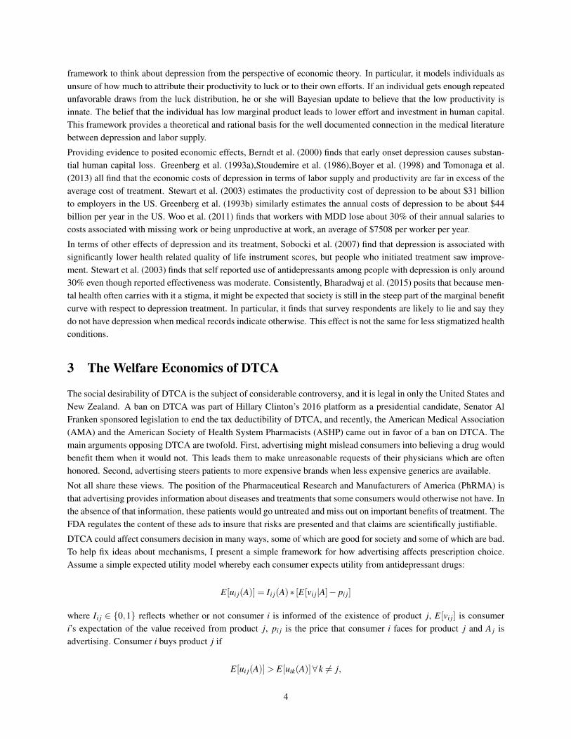
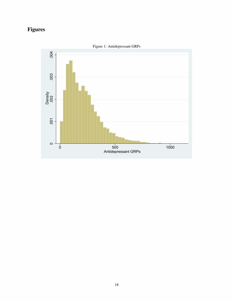
This study focuses on advertisements for the antidepressant drug category. There are many antidepressants, most ofwhich are now generic. The few products that advertise in the data are branded. The primary brands advertisingbetween 2007 and 2010 are Abilify, Cymbalta, Effexor XR, Pristiq and Seroquel XR. While Cymbalta, Effexor XRand Pristiq are all solely used for the treatment of depression, Abilify and Seroquel XR are used both in the treatment ofdepression and in the treatment of psychosis. However, the ad copy description indicates that all Abilify and SeroquelXR advertisements over the course of the data are for the depression indication. The average DMA-month has 227.27GRPs for antidepressants, but with wide dispersion. The standard deviation of DMA-monthly GRPs is 148.67. Ahistogram of DMA-monthly GRP is provided in Figure 1.

4.2 Claims Data

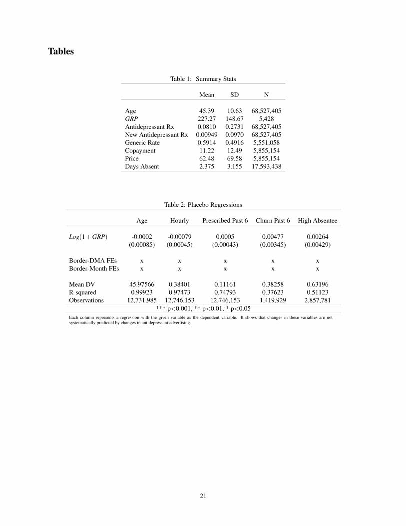
Insurance claims data come from Truven Health MarketScan® Commercial Database which come from Truven HealthAnalytics, Inc., an IBM company. The claims are for individuals with employer sponsored insurance in the UnitedStates that work for companies that are willing to provide the data. From these claims, I harvest prescription anddemographic information on a monthly basis. To make sure I can accurately measure whether a prescription is anew prescription, I focus on those individuals present in the data from the start in January of 2007 and considertheir prescription decisions beginning in February 2007. I define a new prescription as a prescription following amonth with no prescriptions. The final data set that is cleaned and matched to advertising data in the full discoverymarkets contains 1,835,265 individuals with employer sponsored insurance that are on average 45 years old. In anaverage month, 8.1% of the individuals in the data are prescribed an antidepressant, and on average, 59.1% of thoseantidepressant prescriptions are for generics. More summary statistics are available in Table 1.

The claims data also contain information on the transacted prices and co-payments of prescriptions. Co-payments arebased on individual formularies that come with insurance contracts. These contracts typically last a full year, so thereis not variation in co-payments of options for a given individual-month. Similarly, prices reflect the co-payment plusthe payment by the insurance company, as reported by the insurance company. If there are rebates that the insurancecompany receives from the drug manufacturer that are not included in the insurance company’s reported prices, thereported prices would over-state the true cost of a prescription. The contracts between insurance companies and

6

manufacturers also typically last at least a year. As such, all variation within an insurance-contract year in transactedco-payments or prices would reflect variation in choices of different drugs which carry with them different pricesrather than changes in prices for a given drug.

The average price of an antidepressant prescription filled in the data is $61.50 and the average co-payment faced bythe individual enrollee for an antidepressant prescription filled is $11.39.

4.3 Labor Supply Data

Information about worker labor supply is provided from Truven Health MarketScan® Health & Productivity Manage-ment (HPM) database. A subset of the employers who provide the claims data also provide human resources recordson individual enrollee absences from work. Of the individuals in the claims data, there are 518,284 individuals in thelabor supply data between 2007 and 2010.

The average number of missed work days in the data is 2.375 with a standard deviation of 3.155 and a median of 1.25.As missed days can be for any reason, there is a huge amount of month-to-month variation in missed work days, evenwithin individuals. The median number of missed days of 1.25 reflects an average of 3 weeks out of the office peryear, which is a reasonable number for a generally healthy person with two weeks of paid vacation as well as somepaid sick leave.

5 Research Design

There are two main empirical challenges with identifying the effects of advertising on prescriptions, prices and laborsupply in this setting: endogeneity and statistical power. First, as advertising is a firm choice, it is likely targeted atconsumers in a non-random way, in particular towards the potential consumers most likely to be responsive to it. Thosemost likely to be responsive to advertising might also be more likely to get prescribed anyway, eventually receivingany costs or benefits associated with those prescriptions. They could also be more depressed than a randomly selectedtelevision viewer, leading the researcher to find worse outcomes associated with advertising even though the causalityruns the reverse direction.

A second challenge is statistical power, as advertising is thought to have generally small effects and outcomes arenoisy. In particular, workers miss work for many reasons that have nothing to do with depression, advertising orantidepressants. For example, many workers may miss work in a particular area due to a local outbreak of influenza.It would be difficult in the data to know where and when every flu outbreak happens. Even if it happens in a wayindependent of advertising, it will add considerable noise to any estimates of the advertising effect on labor supply.Similar arguments can be made for vacation days, local labor market conditions or weather conditions, for example.An additional complication that exacerbates power issues in this setting is that treatment of depression takes time toproduce individual outcomes. Antidepressants take on average six weeks for improvements to materialize, and thereis considerable variability around that amount of time (Frazer and Benmansour (2002)).

To address these challenges, this study exploits random variation in local advertising generated by the borders ofDMAs. This design was first used in Shapiro (2018) to study the effects of television advertising on antidepressantdemand, but is also used in Tuchman (2016) to study e-cigarette advertising, as well as in Spenkuch and Toniatti(2016) to study political advertising. Consumers who live on different sides of DMA borders face different levels ofadvertising, due to market factors elsewhere in their DMAs. However, these individuals are otherwise similar, makingthe cross-border comparison a clean way to identify the effect of the differential advertising. In this way, at the borders,observed advertising is ‘out of equilibrium’ from what firms would set advertising if they could micro-target very localareas and simulates an experiment.

Capturing this intuition, I estimate the casual effect of advertising on antidepressant prescriptions, prices and laborsupply controlling for unobservable geographic characteristics with border-specific brand-time fixed effects. This

7

allows unobservables to be spatially correlated in ways that are consistent with the evolution of the antidepressantmarket. To control for individual-specific factors that affect antidepressant demand and/or labor supply, individualfixed effects are included. As a number of individual-specific factors and geographic time-specific factors having littleto do with depression affect labor supply, these fixed effects will also help to decrease noise in the dependent variablesof interest.

The top 120 DMAs contain 209 such borders, 163 of which where the border areas make up no more than 35% ofthe total DMA population over the course of this time period. Attention will be restricted to these borders that makeup a smaller fraction of the whole DMA, as in Shapiro (2017). Each of these brand-border pairs will be considered aseparate experiment, with the magnitude of the treatment determined by the advertising in each DMA at a given time,measured in GRPs. Only the individuals residing in counties bordering each other will serve as controls for each otherto partial out any local effects that are correlated with outcomes, including any national advertising. The level of anobservation is an individual-month.

For an illustrative example, Figure 2 shows the Cleveland and Columbus DMAs in the state of Ohio. The borderexperiment considered is outlined in bold. I compare how outcomes on the Cleveland side of the border change whenwhen the Cleveland DMA receives a change in advertising GRPs relative to the Columbus DMA.

5.1 Econometric Model

To model the main effects of advertising on demand, let i index individuals, b index borders, and t index time inmonths. Let Yibdt the outcome of interest for individual i , in border area b , in DMA d, in month t. Let GRPdt indicateadvertising, measured in gross rating points, in DMA d in month t. The effect of an increase in advertising GRP onoutcome Y is estimated with regressions of the form

Yibdt = β1 f1(GRPdt)+β2 f2(t

∑τ=t−t0

GRPτ)+αi +αbt + εibdt , (1)

where β1 and β2 capture the causal effects of current and past advertising, respectively, αi is an individual fixedeffect, αbt is a border area-month fixed effect and εibdt is an econometric error term. I consider the outcomesY ∈ {NewRx, RenewalRx, FirstRenewalRx, Price, Copay, DaysAbsent}. All prescription measures are in terms ofcategory-wide rather than brand-specific. I use two-way clustering to account for two forms of correlation betweenerror terms when computing standard errors. First, conditional on the fixed effect, residual variation in advertising isperfectly correlated at the border-DMA-month. Second, from an experimental design standpoint, there are repeatedmeasurements over time in Y at the individual level. As such, I two-way cluster by border-DMA-month and byindividual (Abadie et al. (2017)).

For the main results, I will set f1(x) = f2(x) = log(1+ x). Additionally, I will consider past advertising to be the sumof GRP for the previous six months. In the case of labor market outcomes, this is to account for the fact that it takestime for outcomes to materialize from depression treatment and that there is variance around exactly how much time.In the case of new prescriptions, allowing lagged advertising to have an effect accounts for advertising carry-over.3

That is, a consumer might watch an ad, but not see the physician for more than a month and at that time remembers lastmonth’s ad. In the case of first renewal prescriptions, I interpret the effect of lagged advertising as indicating whetheror not those who got a new prescription because of advertising in the previous month are more or less likely to churn.That is, it will signify if advertising induces adverse or advantageous selection in terms of propensity to adhere beyondthe first month. In the case of prices and co-payments conditional on a prescription this month, I will set f2 = 0, asthere is no clear theoretical link between past advertising and current transaction prices conditional on treatment.

3However, this should be treated with caution. One can only get a “new” prescription if one did not receive a prescription in the previous month.Getting a large amount of advertising the previous month and nonetheless not getting a prescription suggests a negative epsilon relative to average,which would bias β2 negatively. β2 can alternatively be viewed as a way to control for negative selection into the “new prescription possible”sample for this estimation.

8

For this approach to be useful in identifying advertising effects, two conditions must hold. First, there must besufficient variation in advertising across the borders in the data. If all advertising variation were at the national levelover time and local stations rarely used their discretion to displace national ads, the border-specific time fixed effectswould sweep away all variation in advertising and standard errors would tend to infinity. Second, an individual’slocation with respect to border side must be quasi-random with respect to changes in preferences for antidepressantsand labor supply.

5.2 Features and Limitations

A much more detailed analysis accounting of the features and limitations of the approach is available in both Shapiro(2018) and Shapiro (2017). As the identification strategy in particular is not the main contribution of this study, I willfocus here only on the most important aspects to validity and interpretation.

Perhaps the largest feature of this approach is that the observed advertising levels at the border are quite different thanthey would be if firms micro-targeted advertising at individuals or counties rather than DMAs. That is, the variationat the border is driven by the equilibrium supply and demand in other markets. At the border of the Cleveland, OHDMA, viewers see antidepressant ads that were driven by a desire to reach viewers in metro Cleveland, despite the factthat at the border, these viewers can be quite different. If ads were micro-targeted to the county level, these consumerswould likely see different ads. Similarly, on the Columbus, OH side of the DMA border, the advertising is largelydriven by metro Columbus viewers, which is away from the border, again giving rise to rather different advertisingat the Columbus border than if ads could be micro-targeted. If metro Columbus and metro Cleveland are sufficientlydifferent from each other, these very similar consumers right on the border will get very different ads, even thoughtheir equilibrium micro-targeted ads would have been very similar. This gives a reasonable amount of variation awayfrom what would be the equilibrium in the micro-targeted world while using the fact that these consumers across theborder from one another are very similar to control for unobservable factors driving demand, prices and labor supply.

The border approach has local average treatment effect limitations that are also common to experiments and instru-mental variables. In this case, the estimated effect will be local to those consumers who live in border areas. That is,the ‘compliers’ will be the set of people that live within the border sample, which is a group that can be characterizedand compared with the population at large in a straightforward way. An additional potential limitation to this approachis that it relies crucially on variation in local advertising, which is often a remnant of the upfront market and mightbe systematically different from national network or cable advertising. In this market there is a considerable amountof national advertising, meaning that much of the variation in advertising identifying the effects of interest is awayfrom the zero advertising counterfactual. For an average DMA-month, 7% of the advertising is local advertising, butthere is considerable variation in that, with some DMA-months having no local advertising and some DMA-monthshaving as much as 74%. The standard deviation of the percent of advertising that is local is 13.4%, meaning there isconsiderable variation both in local advertising and in the share of total advertising that is made up by local advertisingin any given DMA-month. To get an idea of the amount of variation in GRPs that is helpful for identification using thisapproach, Figure 3 shows a histogram of GRPs, net of the fixed effects in the border approach, centered at the averageGRP level of 227.27 and winsorized at the 0.1st and 99.9th percentiles. The standard deviation of residual GRPs is 34.

In terms of assessing validity, one approach would be to show that changes in advertising do not predict changes inobservable control variables at the border. Most demographic or industry of work related variables do not changewithin individual over time and are thus taken into account with the individual fixed effects. However, in Table 2, Ishow that the observable variables that do change over time are or are not predicted by changes in current advertisingacross the border. In this table, the reported variable is used as the dependent variable in the specification fromEquation (1). For variables, I use age, whether the worker is paid hourly rather than salary, whether the individualis prescribed in the preceding six months, whether the individual terminates antidepressant treatment conditional onbeing prescribed in the past six months and whether the individual missed more than the population median number of

9

work days in the preceding six months. Current advertising does not predict any of these variables at the p<0.05 level.The only variable that is predicted at the p<0.1 level is the fraction of workers who are paid hourly. On one hand,that estimate could be a false positive. On the other hand, if the point estimate on hourly were to be taken seriously, itwould imply that a 10% increase in advertising would lead to a 0.007 percentage point (or about 0.02%) decrease inthe fraction of workers who are hourly workers, which is economically insignificant.

6 Results

6.1 The Effect of Advertising on Prescriptions

6.1.1 New Prescriptions

Previous research has shown DTCA to be category expansive in the antidepressant category. Here, I test whether thatholds in this data. Table 3 shows the results of estimating equation (1) with new antidepressant prescription as thedependent variable. Column (1) provides estimates from a regression with no controls and no fixed effects, using all ofthe data both at and away from the borders of DMAs. Column (2) adds individual fixed effects, column (3) additionallyadds in month fixed effects and column (4) provides the preferred, border-specification from column (1). Columns (1)and (2) show a small, but statistically significant current advertising effect on new prescriptions and a larger effect ofpast advertising on new prescriptions. The addition of month fixed effects makes those results disappear. In column(4), we see a 10% increase in current antidepressant GRPs leads to about a 0.00031 increase in the probability of a newprescription and past advertising has no effect. As the share of the sample getting a new prescription in a given monthis about 0.0099, this amounts to about a 0.031 elasticity and is in line with the category expansive effect of DTCAfound in Shapiro (2018). The effect of past advertising on new prescriptions, at first blush, suggests that there is nocarry-over effect of advertising. However, that should be interpreted with caution. In order for it to be possible to get anew prescription, one must not have been prescribed in the previous month. Receiving a large treatment of advertisingin the past month but not getting prescribed suggests that this treatment, past advertising plus no past prescription,could be negatively selected.

To get an idea of differential effectiveness by sickness, column (5) presents heterogeneous treatment effects by theaverage number of missed days over the preceding six months, split at the median. That is, if an individual hasmore than the median number of average missed days of work over the previous six months, she is categorized assick. Otherwise, she is categorized as not sick.4 Column (5) shows that I do not have statistical power to distinguishadvertising effects between those who missed a lot of work over the past six months and those who did not miss much.

To obtain dollar social and private costs of the new prescriptions generated by advertising, I assume the average numberof prescriptions resulting from a new prescription, 6, and the average price and co-payments of antidepressants, $62.48and $11.22. Assuming these results apply to all adults in the United States, 230 million, a 10% increase in advertisingleads to 520,000 new antidepressant prescriptions to about 86,500 individuals, which yields approximately $32.4million in total costs of new prescriptions per year, about $5.8 million of which is paid in co-pays by the consumer,assuming no changes in prices or co-payments.5 The 95% confidence interval associated with this cost estimate is[$49,871, $64.4 million].

4As labor supply is only observed for a fraction of the population, we will lose considerable statistical power not just from splitting the sample,but also from missing observations.

5To reach these numbers note that a 10% increase in DTCA corresponds with one tenth the estimated coefficient on log(GRP). The assumed 6months of treatment following an initial prescription is the average observed in the data. So we take one tenth the coefficient on log(GRP) multiplyby 6 months of prescriptions, multiply by the price of a prescription and multiply by twelve months per year.

10

6.1.2 Adherence

Previous studies of DTCA focus on adherence [Donohue et al. (2004); Cardon and Showalter (2015); Wosinska (2005)]and tend to find small, inconsistent and sometimes negative effects of DTCA on adherence. Adherence is an impor-tant consideration for welfare for a few reasons. First, it is possible that advertising reminds patients to refill theirprescriptions appropriately, which would increase the cost of advertising marginal prescriptions, as they would needto be paid for, but also might affect the effectiveness of the eventual treatment. Second, it is possible that advertisinghelps people currently being treated decide that they are poor matches for treatment and convinces them to discontinuetreatment, which would decrease the cost of prescriptions and not worsen welfare outcomes. Third, it is possible thatadvertising reduces adherence inefficiently due to the list of side effects scaring patients off of treatment who shouldcontinue treatment.

Renewal prescriptions are also helpful to identify potential indirect harms of advertising marginal prescriptions. Inparticular, David et al. (2010) and Cardon and Showalter (2015) point out that advertising marginal prescriptions couldbe worse matches than average prescriptions and result in a greater incidence of adverse effects. If this is the case, weshould expect advertising marginal prescriptions to be more likely to be non-adherent in their second month. To testfor this possibility, I assess the effect of past advertising on the first refill of antidepressants. That is, if advertisingcauses a prescription in month t, I want to know if that that prescription is more or less likely to be refilled in periodt +1 than an average prescription.

Table 4 presents the results of the effects of advertising on adherence. Columns (1)-(5) correspond with Table 3 andcolumn (6) presents results on first month adherence. For conciseness, I will only discuss the preferred specifications incolumns (4)-(6). The point estimate on current advertising is negative and small, indicating that it decreases adherenceto treatment with an elasticity of about -0.005. The estimate is statistically significant and very small, consistent withCardon and Showalter (2015), Donohue et al. (2004) and Wosinska (2005).

It is not clear whether the decreased adherence is good or bad. The point estimates in Column (5) imply that thedecreased adherence is coming primarily from those who have recently missed less work, though with considerablyreduced precision and without statistical significance. This is consistent with advertising convincing individuals whostand to gain the least from treatment to discontinue use. This would be the case if, for example, they were prescribedan antidepressant for something less serious than depression, saw the ad, and decided the side effects were not worththe potential gain.

Column (6) presents estimates on first refill adherence. The coefficient of interest is on past advertising, as we wouldlike to know whether or not advertising marginal prescriptions are more or less likely to be refilled. The point estimateis positive, but not statistically significant. This indicates that if anything, the advertising marginal prescriptions aremore likely to be refilled, which is at odds with Cardon and Showalter (2015) and David et al. (2010). That is, theevidence is not consistent with advertising drawing in less appropriate patients. The 95% confidence interval on theelasticity associated with this estimate is [-0.0120, 0.0536], indicating that I can rule out that advertising marginalprescriptions are significantly more likely to be bad matches, but I cannot rule out that the two are identical.

In terms of costs and benefits of adherence, the results indicate that DTCA reduces adherence. This implies a reducedcost of advertising associated with averted prescriptions. The dollar value of one advertising marginal prescriptionaverted is about $62.48. Since 8% of adults are taking antidepressants at any given time, the estimate would applyto about 18.4 million individuals, making the total yearly savings from a 10% increase in DTCA using this measureabout $6 million, or about 97,152 prescriptions. While the point estimates suggested that these averted prescriptionswere primarily coming from those that stood to benefit the least, if some prescriptions are averted wrongly, the cost ofthat will be reflected in the labor supply analysis below.

11

6.2 Prices

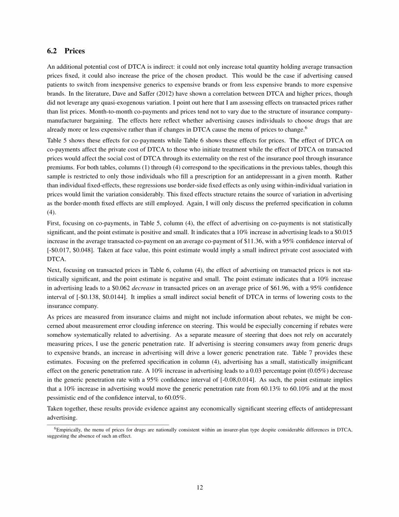
An additional potential cost of DTCA is indirect: it could not only increase total quantity holding average transactionprices fixed, it could also increase the price of the chosen product. This would be the case if advertising causedpatients to switch from inexpensive generics to expensive brands or from less expensive brands to more expensivebrands. In the literature, Dave and Saffer (2012) have shown a correlation between DTCA and higher prices, thoughdid not leverage any quasi-exogenous variation. I point out here that I am assessing effects on transacted prices ratherthan list prices. Month-to-month co-payments and prices tend not to vary due to the structure of insurance company-manufacturer bargaining. The effects here reflect whether advertising causes individuals to choose drugs that arealready more or less expensive rather than if changes in DTCA cause the menu of prices to change.6

Table 5 shows these effects for co-payments while Table 6 shows these effects for prices. The effect of DTCA onco-payments affect the private cost of DTCA to those who initiate treatment while the effect of DTCA on transactedprices would affect the social cost of DTCA through its externality on the rest of the insurance pool through insurancepremiums. For both tables, columns (1) through (4) correspond to the specifications in the previous tables, though thissample is restricted to only those individuals who fill a prescription for an antidepressant in a given month. Ratherthan individual fixed-effects, these regressions use border-side fixed effects as only using within-individual variation inprices would limit the variation considerably. This fixed effects structure retains the source of variation in advertisingas the border-month fixed effects are still employed. Again, I will only discuss the preferred specification in column(4).

First, focusing on co-payments, in Table 5, column (4), the effect of advertising on co-payments is not statisticallysignificant, and the point estimate is positive and small. It indicates that a 10% increase in advertising leads to a $0.015increase in the average transacted co-payment on an average co-payment of $11.36, with a 95% confidence interval of[-$0.017, $0.048]. Taken at face value, this point estimate would imply a small indirect private cost associated withDTCA.

Next, focusing on transacted prices in Table 6, column (4), the effect of advertising on transacted prices is not sta-tistically significant, and the point estimate is negative and small. The point estimate indicates that a 10% increasein advertising leads to a $0.062 decrease in transacted prices on an average price of $61.96, with a 95% confidenceinterval of [-$0.138, $0.0144]. It implies a small indirect social benefit of DTCA in terms of lowering costs to theinsurance company.

As prices are measured from insurance claims and might not include information about rebates, we might be con-cerned about measurement error clouding inference on steering. This would be especially concerning if rebates weresomehow systematically related to advertising. As a separate measure of steering that does not rely on accuratelymeasuring prices, I use the generic penetration rate. If advertising is steering consumers away from generic drugsto expensive brands, an increase in advertising will drive a lower generic penetration rate. Table 7 provides theseestimates. Focusing on the preferred specification in column (4), advertising has a small, statistically insignificanteffect on the generic penetration rate. A 10% increase in advertising leads to a 0.03 percentage point (0.05%) decreasein the generic penetration rate with a 95% confidence interval of [-0.08,0.014]. As such, the point estimate impliesthat a 10% increase in advertising would move the generic penetration rate from 60.13% to 60.10% and at the mostpessimistic end of the confidence interval, to 60.05%.

Taken together, these results provide evidence against any economically significant steering effects of antidepressantadvertising.

6Empirically, the menu of prices for drugs are nationally consistent within an insurer-plan type despite considerable differences in DTCA,suggesting the absence of such an effect.

12

6.3 Labor Supply

To assess the potential benefits of DTCA, I estimate equation (1) using missed days of work as the dependent variable.7

In this case, any potential effects of DTCA on labor supply would be expected to manifest with a lag, as antidepressantsdo not work instantaneously. As such, the coefficient of interest is the one attached to lagged DTCA.

In terms of concerns over endogeneity in a naive correlational analysis, firms might well direct their advertising mostat places where individuals have a high incidence of depression. If that is the case, we would find a spurious positiveeffect of current DTCA on current missed days of work. As many of these individuals might get treated with or withoutthe advertising, we would find a spurious negative effect of past DTCA on current missed days of work if treatmentwere effective.

Table 8 presents the labor supply results. Column (1) provides the naive regression with no controls and no fixedeffects. It indicates that work days missed are significantly increased by current DTCA and significantly decreased bypast DTCA. These results are directionally consistent with the expected spurious result. In column (2), individual fixedeffects are included. Both effects persist, but the effect of past DTCA is muted to some degree. In column (3), monthfixed effects are added, which control for seasonal factors that are correlated with labor supply. For example, manyfamilies go on vacation during December or July. With the inclusion of month fixed effects, the estimate on currentDTCA changes sign and becomes insignificant. The estimate on past DTCA persists, but is no longer statisticallysignificant. These two forces highlight the two main empirical concerns. First, it seems firms are targeting ads toplaces where they expect individuals are missing a lot of work, and second, there is a lot of variation in month overmonth labor supply that has little to do with antidepressant DTCA and that generates significant noise. Column (4)addresses both of these concerns by implementing the border strategy from equation (1). Despite losing 80% of theobservations by focusing only on the borders, standard errors decrease considerably. The border-month fixed effectssoak up significant variation in labor supply that has nothing to do with antidepressant DTCA. Current DTCA hasno significant effect on days missed, but the point estimate is small and negative. Past DTCA has a significant andnegative effect on days missed, suggesting that not only does advertising increase new prescriptions, it eventually leadsto individuals missing less work. The point estimate is consistent with an elasticity of labor supply with respect toadvertising of about 0.05. Column (5) shows that this effect appears to be coming from those who have missed a lotof work in the previous six months.

I note here that I cannot statistically distinguish the estimates in column (3) from the estimates in column (4). Thisis partially due to the large amount of noise in the estimates in column (3), but it is also consistent with the panelstructure of the data and individual and month fixed effects being sufficient to remove contamination, while the borderstrategy adds additional statistical power. I will proceed using the estimates in column (4) as the preferred estimates,as they are the both the most conservative with respect to controlling for confounds and exhibit the most statisticalpower.

The point estimate of column (4) of -0.1382 indicates the average individual in the sample gains about 0.11 hoursof monthly time at work from a 10% increase in the past 6 months of DTCA. Assuming this number applies to allworking adults (about 145 million) and assuming the national average wage of $24/hour8, a sustained 10% increasein DTCA for a year would lead to $769.5 million in increased wage benefits, or about $5.31 per working adult. If weassume this benefit only applies to those who are advertising marginal to new prescriptions (about 86,500 individuals,as noted above), those individuals gain about 3.86 work days per month and $8,900 per year, or about 18% of theirannual incomes, on average, which is just under half of the effect of depression on annual earnings reported by Wooet al. (2011). With average co-payments of $11.22 and 6 months of treatment, the private cost to obtain the $8,744in benefits is about $67. With the average transaction price of $62.48, the total cost is $375.9 Of course it is possible

7Using log(absent hours) instead of level of missed days does not change the results significantly quantitatively or qualitatively. Those resultswill eventually be provided in an appendix.

8I note here that using $24 as the basis for the social hourly benefit of work assumes that workers are paid their marginal product of labor. Ifemployers have market power in the labor market and pay workers less than their marginal products, this will leave out benefits to employers.

9To reach these numbers note that a 10% increase in DTCA corresponds with one tenth the estimated coefficient on log(Past GRP). Since past

13

that the effect of DTCA on labor supply acts not only through new prescriptions, but also through other mechanisms.For example, the decreased adherence among the poorly suited could generate labor supply due to the elimination ofadverse effects, individuals could seek non-drug treatment of their depression after seeing ads or individuals couldsimply be more cognizant of depressive tendencies, leading to increased labor supply.10

The 95% confidence interval on the total yearly benefits of a 10% increase in DTCA is [$112.6 million, $1.427 billion].The 95% confidence interval on the yearly costs of marginal prescriptions from a 10% increase in DTCA was [$49,871,$64.4 million], indicating that the cost and benefit confidence intervals do not overlap. Assuming the highest cost andlowest benefit still puts the benefits at nearly double the cost.

6.4 Unmeasured costs and benefits

It should be noted that some possible costs and benefits of DTCA are either not measured in this study or do not comewith easily calculable dollar values.

In terms of unmeasured benefits, some individuals may have no change in labor supply, but are more productivewhile they are at work due to being treated. Additionally, some people might simply feel better, and that could haveconsiderable value, but by how much in dollars is unclear. Furthermore, wage dollars represent a strict lower bound onthe cost of absenteeism. If employers have market power in the labor market, they are likely to pay their workers lessthan their marginal product of labor. As such, any measurement using wage dollars alone will understate the socialbenefit of reduced absenteeism.

In terms of costs that I do not measure, while advertising marginal drugs bring with them marginal benefits of laborsupply, they may also bring with them marginal costs of adverse effects that do not fully manifest themselves in laborsupply reductions. This would be the case if an individual was able to go to work more, but also had more headaches,which could be privately costly as well as make the employee less productive for the employer. Of course, there isfree disposal of a prescription. If the benefit of feeling better does not outweigh the pain of adverse effects, then thepatient could discontinue use, or rationally not adhere to treatment.

Additionally, some people may directly dislike watching television ads for antidepressants (see, for example, Wilburet al. (2013)). If the alternative to antidepressant DTCA were additional television programming, the effect mightbe significant. However, if we were to remove antidepressant DTCA, it is much more likely the viewer would get adifferent advertisement, which would imply a smaller welfare effect.

Assuming no unmeasured benefits of DTCA, those costs would have to add up to at least $737 million per 10%increase in antidepressant DTCA in order to flip this cost-benefit analysis.

How big is a 10% increase in DTCA? As mentioned above, in 2012, the total antidepressant DTCA expenditure was$300 million, so a 10% sustained increase would be an increase in DTCA spending of $30 million per year.11 In thecontext of private firms spending money on advertising, this $30 million in expenditure is a transfer from the advertiserto the television network from a welfare perspective. However, if a government or charitable organization wanted tobegin a campaign of advertising for depression treatment and thought it could get similar results as found here, $30million is quite small in comparison with the $769.5 million in measured benefit for that money.

GRP is defined as 6 months past, the estimate must be divided by 6 to avoid double counting. Then, it is multiplied by 8 hours per day, by $24 perhour, by 12 months in a year and by 145 million working adults to arrive at the final estimate. To obtain the estimate on only those marginal toprescriptions, I take the $769.5 million and divide it by the 88,000 individuals estimated to be advertising marginal to prescriptions in a year.

10Separation of these mechanisms is difficult due to statistical power limitations, but continuing work on this study is attempting to better separatethe mechanisms.

11It is interesting to note that the estimated DTCA-marginal revenue was about $32.6 million, making a 10% increase in DTCA about 8.7% ROI, not accounting for the decreased adherence, which was marginally significant. These numbers suggest the estimated effects on prescriptions areplausible in terms of the firm’s first order condition.

14

6.5 Cautions & Limitations

The reader should take some caution in interpreting these results for policy. First and foremost, they only apply toDTCA as it relates to antidepressant treatment. DTCA for another drug category might have a different interactionwith patient selection on potential to gain from treatment. Depression is thought by many physicians to be under-treated due to the stigmatization, which leaves plenty of opportunity for welfare increasing market expansion. Forcholesterol lowering drugs or erectile dysfunction drugs, that might be quite different. However, these estimates doprovide evidence that a blanket ban on all DTCA might be a bad idea.

Second, the border identification strategy identifies an effect local to the borders of television markets. It is possiblethat the true effect of advertising away from the borders of TV markets is different from the effect at the border. Onereason to potentially worry less about this is that the specification using all of the data, including away from the borderwith month and individual fixed effects is consistent with the result at the border, but with more noise. Additionally,there are many borders in this data with many types of individuals. For the non-border counties to flip the cost-benefitin this case would require drastically different advertising effects, both on labor supply and on prescriptions. Theeffect on prescriptions would need to be much larger and the effect on labor supply much smaller.

Third, all calculations on costs and benefits are computed at the point estimates, but each of these are functions ofestimated values with standard errors. Taking a pessimistic view of both the benefits and using the 5% end of theconfidence interval for labor supply results and a 95% end of the confidence interval for new prescriptions, the benefitsstill outweigh the costs, but the gap between them is considerably muted. For a 10% increase in DTCA using thesemaximally pessimistic estimates, cost of new prescriptions is $64.4 million and the benefit of those prescriptions is$112.6 million.

7 Conclusion

In this paper, I find substantial benefits of antidepressant DTCA on labor supply. The effects are plausible in magnitudeat the individual level, with the marginal prescribed individual gaining about 3.78 days of work per month or $8,744annually from the advertising marginal treatment that comes from a 10% increase in DTCA. The total wage benefits oflabor supply from a 10% increase in DTCA, at $769.5 million are substantially larger than the $32.4 million in directcosts of the marginal prescriptions generated. Indirect costs that can be easily assigned a dollar value, increases in co-payments and prices, are shown to be small and statistically insignificant, which indicates DTCA does not significantlysteer patients to more expensive treatments. Additional savings come from reduced adherence among those who standto gain little in the form of increased labor supply. In terms of costs and benefits without clear dollar values, I findevidence that DTCA does not produce worse matches and might even produce better matches with treatment, as thosewith exposed to high past advertising are marginally more likely to adhere to their first refill than are those exposed tolower past advertising.

These results highlight the importance of understanding which types of consumers are affected by advertising andmeasuring how much these consumers benefit from marginal treatment when assessing the desirability of DTCA. Inthe case of antidepressants, the marginal consumers stand to gain and do gain from treatment in a way that far exceedsthe social cost. While this result might not be the same across different drug categories, it highlights that a morenuanced approach than a blanket ban on DTCA might be desirable.

References

Abadie, A., Athey, S., Imbens, G. W., and Wooldridge, J. (2017). When should you adjust standard errors for cluster-ing? Technical report, National Bureau of Economic Research.

15

Aizawa, N. and Kim, Y. S. (2018). Advertising and risk selection in health insurance markets. American EconomicReview, forthcoming.

Alpert, A., Lakdawalla, D., and Sood, N. (2015). Prescription drug advertising and drug utilization: the role ofmedicare part d. Technical report, National Bureau of Economic Research.

Berndt, E. R., Koran, L. M., Finkelstein, S. N., Gelenberg, A. J., Kornstein, S. G., Miller, I. M., Thase, M. E., Trapp,G. A., and Keller, M. B. (2000). Lost human capital from early-onset chronic depression. American Journal ofPsychiatry, 157(6):940–947.

Bharadwaj, P., Pai, M. M., and Suziedelyte, A. (2015). Mental health stigma. NBER Working Paper 21240.

Boyer, P., Danion, J., Bisserbe, J., Hotton, J., and Troy, S. (1998). Clinical and economic comparison of sertraline andfluoxetine in the treatment of depression. Pharmacoeconomics, 13(1):157–169.

Bütikofer, A. and Skira, M. M. (2016). Missing work is a pain: The effect of cox-2 inhibitors on sickness absence anddisability pension receipt. Journal of Human Resources, pages 0215–6958R1.

Cardon, J. H. and Showalter, M. H. (2015). The effects of direct-to-consumer advertising of pharmaceuticals onadherence. Applied Economics, 47(50):5432–5444.

Chesnes, M. and Jin, G. Z. (2016). Direct-to-consumer advertising and online search.

Currie, J. and Madrian, B. C. (1999). Health, health insurance and the labor market. Handbook of labor economics,3:3309–3416.

Dave, D. and Saffer, H. (2012). Impact of direct-to-consumer advertising on pharmaceutical prices and demand.Southern Economic Journal, 79(1):97–126.

David, G., Markowitz, S., and Richards-Shubik, S. (2010). The effects of pharmaceutical marketing and promotionon adverse drug events and regulation. American Economic Journal: Economic Policy, 2(4):1–25.

De Quidt, J. and Haushofer, J. (2016). Depression for economists. Technical report, National Bureau of EconomicResearch working paper 22973.

Deshpande, M. (2016). Does welfare inhibit success? the long-term effects of removing low-income youth from thedisability rolls. The American Economic Review, 106(11):3300–3330.

Donohue, J. M., Berndt, E. R., Rosenthal, M., Epstein, A. M., and Frank, R. G. (2004). Effects of pharmaceuticalpromotion on adherence to the treatment guidelines for depression. Medical care, 42(12):1176–1185.

Frazer, A. and Benmansour, S. (2002). Delayed pharmacological effects of antidepressants. Molecular psychiatry,7(S1):S23.

Garthwaite, C. L. (2012). The economic benefits of pharmaceutical innovations: the case of cox-2 inhibitors. AmericanEconomic Journal: Applied Economics, 4(3):116–137.

Greenberg, P. E., Stiglin, L. E., Finkelstein, S. N., and Berndt, E. R. (1993a). Depression: a neglected major illness.The Journal of clinical psychiatry.

Greenberg, P. E., Stiglin, L. E., Finkelstein, S. N., and Berndt, E. R. (1993b). The economic burden of depression in1990. The Journal of clinical psychiatry.

Grundl, S. and Kim, Y. J. (2017). Consumer mistakes and advertising: The case of mortgage refinancing.

16

Iizuka, T. and Jin, G. Z. (2005). The effect of prescription drug advertising on doctor visits. Journal of Economics &Management Strategy, 14(3):701–727.

Iizuka, T. and Jin, G. Z. (2007). Direct to consumer advertising and prescription choice. Journal of IndustrialEconomics, 55(4):771–771.

Kim, T. and KC, D. S. (2017). Can viagra advertising make more babies?

Niederdeppe, J., Avery, R. J., Kellogg, M. D., and Mathios, A. (2017). Mixed messages, mixed outcomes: Exposureto direct-to-consumer advertising for statin drugs is associated with more frequent visits to fast food restaurants andexercise. Health Communication, 32(7):845–856. PMID: 27428179.

Shapiro, B. (2017). Advertising in health insurance markets. Marketing Science, forthcoming.

Shapiro, B. T. (2018). Positive spillovers and free riding in advertising of prescription pharmaceuticals: The case ofantidepressants. Journal of Political Economy, 126(1):381–437.

Sinkinson, M. and Starc, A. (2017). Ask your doctor? direct-to-consumer advertising of pharmaceuticals. Review ofEconomic Studies, forthcoming.

Sobocki, P., Ekman, M., Ågren, H., Krakau, I., Runeson, B., Mårtensson, B., and Jönsson, B. (2007). Health-relatedquality of life measured with eq-5d in patients treated for depression in primary care. Value in Health, 10(2):153–160.

Spenkuch, J. L. and Toniatti, D. (2016). Political advertising and election outcomes.

Stewart, W. F., Ricci, J. A., Chee, E., Hahn, S. R., and Morganstein, D. (2003). Cost of lost productive work timeamong us workers with depression. Journal of the American Medical Association, 289(23):3135–3144.

Stoudemire, A., Frank, R., Hedemark, N., Kamlet, M., and Blazer, D. (1986). The economic burden of depression.General Hospital Psychiatry, 8(6):387–394.

Tomonaga, Y., Haettenschwiler, J., Hatzinger, M., Holsboer-Trachsler, E., Rufer, M., Hepp, U., and Szucs, T. D.(2013). The economic burden of depression in switzerland. Pharmacoeconomics, 31(3):237–250.

Tuchman, A. E. (2016). Advertising and demand for addictive goods: The effects of e-cigarette advertising. Technicalreport.

Wilbur, K. C., Xu, L., and Kempe, D. (2013). Correcting audience externalities in television advertising. MarketingScience, 32(6):892–912.

Woo, J.-M., Kim, W., Hwang, T.-Y., Frick, K. D., Choi, B. H., Seo, Y.-J., Kang, E.-H., Kim, S. J., Ham, B.-J., Lee,J.-S., et al. (2011). Impact of depression on work productivity and its improvement after outpatient treatment withantidepressants. Value in Health, 14(4):475–482.

Wosinska, M. (2005). Direct-to-consumer advertising and drug therapy compliance. Journal of Marketing Research,42(3):323–332.

17

Figures

Figure 1: Antidepressant GRPs0

.001

.002

.003

.004

Den

sity

0 500 1000Antidepressant GRPs

18

Figure 2: Ohio and DMA Border Example

19

Figure 3: Antidepressant DTCA GRP variation across Borders

0.0

1.0

2.0

3.0

4.0

5D

ensi

ty

0 100 200 300 400 500GRPs net of Fixed Effects

20

Tables

Table 1: Summary Stats

Mean SD N

Age 45.39 10.63 68,527,405GRP 227.27 148.67 5,428Antidepressant Rx 0.0810 0.2731 68,527,405New Antidepressant Rx 0.00949 0.0970 68,527,405Generic Rate 0.5914 0.4916 5,551,058Copayment 11.22 12.49 5,855,154Price 62.48 69.58 5,855,154Days Absent 2.375 3.155 17,593,438

Table 2: Placebo Regressions

Age Hourly Prescribed Past 6 Churn Past 6 High Absentee

Log(1+GRP) -0.0002 -0.00079 0.0005 0.00477 0.00264(0.00085) (0.00045) (0.00043) (0.00345) (0.00429)

Border-DMA FEs x x x x xBorder-Month FEs x x x x x

Mean DV 45.97566 0.38401 0.11161 0.38258 0.63196R-squared 0.99923 0.97473 0.74793 0.37623 0.51123Observations 12,731,985 12,746,153 12,746,153 1,419,929 2,857,781

*** p<0.001, ** p<0.01, * p<0.05Each column represents a regression with the given variable as the dependent variable. It shows that changes in these variables are notsystematically predicted by changes in antidepressant advertising.

21

Table 3: New Prescriptions

(1) (2) (3) (4) (5)

Log(1+GRP) 0.00011*** 0.00008** 0.00004 0.00031* 0.00046(0.00003) (0.00003) (0.00005) (0.00015) (0.00060)

xHighAbsentee 0.00037(0.00060)

Log(1+GRPpast) 0.00076*** 0.00050*** -0.0001 -0.00019 0.00066(0.00022) (0.00005) (0.00007) (0.00027) (0.00101)


Individual FEs x x x xMonth FEs xBorder-Month FEs x x


*** p<0.001, ** p<0.01, * p<0.05Standard errors are two-way clustered. First, they are clustered by (border)x(DMA)x(Month) to account for correlation in thetreatment variable. Second, they are clustered by individual to account for the fact that there are repeated observations withinindividual over the sample.

22

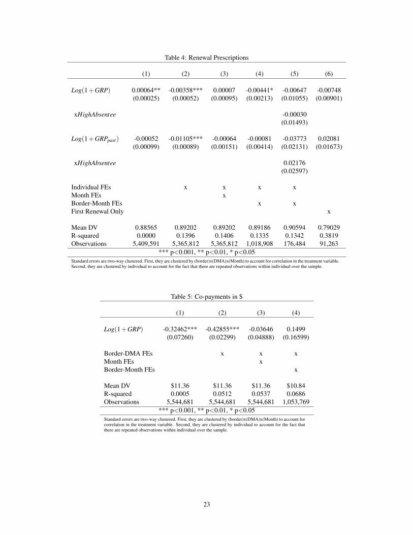
Table 4: Renewal Prescriptions

(1) (2) (3) (4) (5) (6)

Log(1+GRP) 0.00064** -0.00358*** 0.00007 -0.00441* -0.00647 -0.00748(0.00025) (0.00052) (0.00095) (0.00213) (0.01055) (0.00901)

xHighAbsentee -0.00030(0.01493)

Log(1+GRPpast) -0.00052 -0.01105*** -0.00064 -0.00081 -0.03773 0.02081(0.00099) (0.00089) (0.00151) (0.00414) (0.02131) (0.01673)


Individual FEs x x x xMonth FEs xBorder-Month FEs x xFirst Renewal Only x

Mean DV 0.88565 0.89202 0.89202 0.89186 0.90594 0.79029R-squared 0.0000 0.1396 0.1406 0.1335 0.1342 0.3819Observations 5,409,591 5,365,812 5,365,812 1,018,908 176,484 91,263

*** p<0.001, ** p<0.01, * p<0.05Standard errors are two-way clustered. First, they are clustered by (border)x(DMA)x(Month) to account for correlation in the treatment variable.Second, they are clustered by individual to account for the fact that there are repeated observations within individual over the sample.

Table 5: Co-payments in $

(1) (2) (3) (4)

Log(1+GRP) -0.32462*** -0.42855*** -0.03646 0.1499(0.07260) (0.02299) (0.04888) (0.16599)

Border-DMA FEs x x xMonth FEs xBorder-Month FEs x

Mean DV $11.36 $11.36 $11.36 $10.84R-squared 0.0005 0.0512 0.0537 0.0686Observations 5,544,681 5,544,681 5,544,681 1,053,769

*** p<0.001, ** p<0.01, * p<0.05Standard errors are two-way clustered. First, they are clustered by (border)x(DMA)x(Month) to account forcorrelation in the treatment variable. Second, they are clustered by individual to account for the fact thatthere are repeated observations within individual over the sample.

23

Table 6: Transaction Price in $

(1) (2) (3) (4)

Log(1+GRP) -0.54284** -0.74045*** 0.14356 -0.61605(0.20638) (0.07722) (0.12612) (0.38631)


Mean DV $62.78 $62.78 $62.78 $61.96R-squared 0.00004 0.01033 0.01116 0.02373Observations 5,544,681 5,544,681 5,544,681 1,053,769

*** p<0.001, ** p<0.01, * p<0.05Standard errors are two-way clustered. First, they are clustered by (border)x(DMA)x(Month) to account forcorrelation in the treatment variable. Second, they are clustered by individual to account for the fact that thereare repeated observations within individual over the sample.

Table 7: Generic Penetration Rate

(1) (2) (3) (4)

Log(1+GRP) 0.01983*** 0.02454*** -0.00184 -0.00335(0.00199) (0.00099) (0.00102) (0.00246)


Mean DV 0.59145 0.59145 0.59145 0.59867R-squared 0.00109 0.01629 0.02045 0.03573Observations 5,551,058 5,551,058 5,551,058 1,054,561

*** p<0.001, ** p<0.01, * p<0.05Standard errors are two-way clustered. First, they are clustered by (border)x(DMA)x(Month) to account forcorrelation in the treatment variable. Second, they are clustered by individual to account for the fact that thereare repeated observations within individual over the sample.

24

Table 8: Labor Supply - Missed Days of Work

(1) (2) (3) (4) (5)

Log(1+GRP) 0.2100* 0.2518** -0.0650 -0.0339 -0.0066(0.0990) (0.0768) (0.0904) (0.0288) (0.0255)


Log(1+GRPpast) -0.5356 -0.3710* -0.2757 -0.1382* -0.05923(0.2886) (0.1477) (0.1830) (0.0602) (0.0519)

xHighAbsentee -.2086(0.12134)




Appendix A - Log Hours

In this appendix, I consider the alternative dependent variable of the log of absentee hours per month. As such, theseestimates can be read directly as elasticities of labor supply with respect to advertising. The results are presented inTable A.1 are consistent with the main results using levels rather than logs. In particular, in columns (1) and (2),the correlation between current DTCA and labor supply indicates that advertising increases absenteeism, which is aspurious result if firms are targeting advertising at places and during times when individuals are likely to miss a lotof work. In columns (1) and (2), past advertising is negatively correlated with labor supply, but the estimates are notespecially precise. In column (3), the positive correlation between absenteeism and current advertising disappears andthe magnitude of the point estimate on past advertising decreases and becomes statistically insignificant. In column(4), moving to the borders does not change the point estimates in a meaningful way, but considerable precision isgained, making this column my preferred specification for this table. It indicates that current advertising does notaffect absenteeism while the elasticity of labor supply with respect to past advertising is about -0.045, quantitativelyconsistent with the main results using levels as the dependent variable. Column (5) shows that the labor supply resultis driven entirely by those who miss the most days on average. All in all, the results using log of absent hours as thedependent variable do not differ qualitatively or quantitatively from the results using absentee days as the dependentvariable.

25

Table A.1: Labor Supply - Log of Absent Hours

(1) (2) (3) (4) (5)

Log(1+GRP) 0.09429*** 0.11331*** -0.01139 -0.00636 -0.00222(0.0255) (0.0291) (0.0290) (0.0124) (0.0146)


Log(1+GRPpast) -0.16632 -0.11521** -0.04367 -0.04483* 0.01748(0.0927) (0.0434) (0.0422) (0.0211) (0.0308)

xHighAbsentee -0.0783*(0.0391)




Appendix B - Outcome Timing

As noted above, antidepressants are not expected to work immediately upon prescription. While on average they takeabout six weeks to work, there is variance around that mean and those who are newly prescribed often take the drugsfor a number of months. This is why the conception of past advertising used in the main results is the sum of the pastsix months of advertising. In this appendix, I relax that parametric assumption and look at each lag of advertisingseparately. If six weeks is in fact the average amount of time needed for antidepressants to work, the effects should bestrongest for advertising that is lagged two months with possible effects continuing in later months minimal effects incurrent and one month lagged advertising. Given the limited statistical power generally, it is difficult to be say muchwith precision, however.

The results of this analysis are in Table B.1. In the first column, this analysis is conducted with absentee days as thedependent variable. The largest point estimate is on advertising two months lagged. It is not sufficiently precise to bestatistically significant at the p<0.05 level and has p-value of about 0.08. Power is too limited to say much beyond that.In the second column, log of absent hours is the dependent variable. In that column we again face very limited power.However, the effects on two and three month lagged advertising are the largest negative effects, with longer lags alsobeing similarly negative with the exception of five months lagged being positive. In both columns, the effects on thecurrent and one month lagged advertising are the smallest and indicate little or no effect, which is what we shouldexpect from the science of antidepressant effectiveness. While getting the exact nature of the lagged effectivenessproves too challenging in this context due to statistical power, it is reassuring that the effects of lagged advertising onlabor supply are not manifesting themselves in the current and one month lagged advertising variable, which wouldindicate a likely spurious result.

26

Table B.1: Outcome Timing

Days Log Hours

Log(1+GRP) -0.00004 0.00084(0.0352) (0.0144)

Log(1+GRPt−1) -0.03532 0.00148(0.0577) (0.0164)

Log(1+GRPt−2) -0.11019 -0.01673(0.0623) (0.0168)

Log(1+GRPt−3) -0.00116 -0.01578(0.0299) (0.0149)

Log(1+GRPt−4) -0.0046 0.0232(0.0425) (0.0145)

Log(1+GRPt−5) -0.01051 -0.00845(0.0351) (0.0145)

Log(1+GRPt−6) 0.00008 -0.01199(0.0264) (0.0133)

Individual FEs x xBorder-Month FEs x x

Mean DV 2.262 2.505R-squared 0.00331 0.3622Observations 2,984,534 2,984,534

*** p<0.001, ** p<0.01, * p<0.05Standard errors are two-way clustered. First, they are clustered by (bor-der)x(DMA)x(Month) to account for correlation in the treatment vari-able. Second, they are clustered by individual to account for the factthat there are repeated observations within individual over the sample.

Appendix C - Selection into the Border Sample

In this section, I measure how the border sample used for the preferred specifications is different the non-border samplein terms of observables in the data. I do this at a single point in time, July 2007 and test the null hypothesis that thedifference in means is zero. The variables examined are percent of population employed in manufacturing (broadlydefined), age, the percent of the population paid hourly (as opposed to salaried), the percent of the population that wasprescribed an antidepressant in the previous six months, the percent of the population that was both prescribed in thepast six months and failed to adhere, average missed days per month, and antidepressant prices and co-pays conditionalon prescription. The results are in Table C.1. Most of the differences are statistically significant given the large samplesize, but not all are economically large. Notable economically large differences include the borders having a higherpercentage manufacturing jobs and individuals missing more work per month on average . Statistically significant,but smaller differences include the borders being slightly older, slightly more likely to be paid hourly, slightly morelikely to be prescribed an antidepressant in the past six months and slightly lower cost antidepressants being chosenconditional on purchase, both in prices and co-pays. There is no detectable difference between the border and non-border counties in propensity to adhere to treatment.

In addition to this, Shapiro (2017) shows that border counties tend to be older, less populous, less wealthy and lessracially diverse. None of these differences provide sharp predictions about differences in treatment effects of advertis-ing on sales or outcomes, however. In fact, the simple diff-in-diff specifications of the effect of advertising on laborsupply outcomes fail to reject equality with the border approach treatment effects.

27

Table C.1: Selection into the Border Sample

Mean Border Mean Non-Border Difference P-Value

% Manufacturing 66.47 54.05 12.41 <0.01Age 44.62 43.46 1.158 <0.01% Hourly 37.95 36.08 1.862 <0.01% Prescribed Past 6 11.47 10.51 0.959 <0.01% Non-Adherence Past 6 42.38 42.14 0.238 0.444Avg Absentee Days 2.989 2.359 0.630 <0.01Price 60.86 62.78 1.92 <0.01Copay 11.47 12.25 0.78 <0.01

P-value comes from a t-test with null hypothesis of zero difference between means

28

Documents

Promoting Wellness or Waste? Evidence from Antidepressant Advertising€¦ · · 2 days agoPromoting Wellness or Waste? Evidence from Antidepressant ... using individual health