Vol.:(0123456789)1 3

Clim Dyn DOI 10.1007/s00382-017-3624-y

Prolonged effect of the stratospheric pathway in linking Barents–Kara Sea sea ice variability to the midlatitude circulation in a simplified model

Pengfei Zhang1  · Yutian Wu1 · Karen L. Smith2 

Received: 16 November 2016 / Accepted: 6 March 2017 © Springer-Verlag Berlin Heidelberg 2017

Keywords Stratosphere–troposphere coupling · Nudging method · Planetary-scale wave propagation · Barents–Kara Sea sea ice · Midlatitude low-level jet · Cold advection over central Asia

1 Introduction

Previous studies have found that Arctic sea ice variabil-ity and the resulting temperature perturbation, especially over the Barents–Kara Sea (BKS), can strongly affect the Northern Hemisphere (NH) midlatitude circulation, such as the westerly jet and planetary-scale waves, and possibly blocking frequency and Eurasian cold spells (e.g., Honda et  al. 2009; Francis and Vavrus 2012; Cohen et  al. 2014; Mori et  al. 2014; Vihma 2014; Barnes and Screen 2015; Hassanzadeh and Kuang 2015; Kug et al. 2015; Lee et al. 2015; Screen et al. 2015). From observations, sea ice vari-ability over the entire Arctic has been found to precede the anomalous wintertime tropospheric circulation by about 2–4 months (Wu and Zhang 2010). Over the BKS region, the sea ice variability maximizes in autumn (not shown), with November (Nov) sea ice exerting the largest impact on the midlatitude circulation in the subsequent winter (Koenigk et  al. 2016; Yang et  al. 2016). Figure 1a shows the regression of surface air temperature (SAT) on the Nov BKS sea ice concentration (SIC) after removing the long-term trend and the El Niño-Southern Oscillation (ENSO) related component (data and calculation details can be found in Sect. 2). Significant anomalous warm SAT associ-ated with lower than normal BKS SIC can be seen in Nov and December (Dec) over the BKS region. The maximum SAT difference is about 9  K between low and high Nov BKS SIC index years (defined by exceeding ±0.8 standard deviation). The response of the NH midlatitude jet stream,

Abstract To better understand the dynamical mechanism that accounts for the observed lead-lag correlation between the early winter Barents–Kara Sea (BKS) sea ice variabil-ity and the later winter midlatitude circulation response, a series of experiments are conducted using a simplified atmospheric general circulation model with a prescribed idealized near-surface heating over the BKS. A prolonged effect is found in the idealized experiments following the near-surface heating and can be explicitly attributed to the stratospheric pathway and the long time scale in the strato-sphere. The analysis of the Eliassen-Palm flux shows that, as a result of the imposed heating and linear constructive interference, anomalous upward propagating planetary-scale waves are excited and weaken the stratospheric polar vortex. This stratospheric response persists for approxi-mately 1–2  months accompanied by downward migration to the troposphere and the surface. This downward migra-tion largely amplifies and extends the low-level jet deceler-ation in the midlatitudes and cold air advection over central Asia. The idealized model experiments also suggest that the BKS region is the most effective in affecting the mid-latitude circulation than other regions over the Arctic.

Electronic supplementary material The online version of this article (doi:10.1007/s00382-017-3624-y) contains supplementary material, which is available to authorized users.

* Pengfei Zhang zpengfei@purdue.edu

1 Department of Earth, Atmospheric and Planetary Sciences, Purdue University, West Lafayette, IN, USA

2 Lamont-Doherty Earth Observatory, Columbia University, Palisades, NY, USA

P. Zhang et al.

1 3

however, is not synchronized with the SAT anomaly but rather is maximized over the North Atlantic-Europe sector during January (Jan) and February (Feb) (Fig. 1b), which is about 2–3 months after the Nov BKS SIC variability and about 1–2 months after the SAT perturbation. However, the dynamical mechanism that accounts for this lead-lag rela-tionship has not yet been fully explored.

Stratospheric processes, whose time scales are longer than that of the troposphere (e.g., Baldwin et  al. 2003), may provide a possible explanation. Recent studies have suggested an important role of the stratospheric pathway in linking the Arctic with the midlatitude circulation via upward wave propagation and downward migration (Sun et  al. 2015; Nakamura et  al. 2016; Wu and Smith 2016). The enhanced upward propagating planetary-scale waves due to sea ice loss could penetrate into the stratosphere, increase the geopotential height and decelerate the west-erly in the stratosphere, and thus weaken the stratospheric

polar vortex (Jaiser et  al. 2013; Kim et  al. 2014). These stratospheric circulation responses are likely to persist in the stratosphere for a couple of months accompanied by downward migration back to the troposphere and the sur-face (Kim et  al. 2014; Sun et  al. 2015; Nakamura et  al. 2016). This is in addition to the tropospheric pathway that involves transient eddy adjustment to change in meridional temperature gradient (Deser et  al. 2004). Previous stud-ies (Sun et al. 2015; Nakamura et al. 2016; Wu and Smith 2016) have suggested that the stratospheric pathway could be as important as the tropospheric pathway in influencing the midlatitude circulation; however, no previous work, to the best of our knowledge, has explicitly quantified the role of the stratospheric pathway in linking the early winter sea ice variability with the later winter midlatitude circulation.

In this study we aim to address the following ques-tions: What is responsible for the 1–2 months lag between the BKS temperature perturbation and NH midlatitude

(a)

(b)

Fig. 1 Regression of surface air temperature (SAT, units: K) in November and December on the normalized November BKS SIC (a). b is the same as a but for 700 hPa zonal wind (color shading, units: m s−1) in December, January and February. Stippling denotes the 95% confidence level. The black curves in a mark the BKS region. The

dashed lines in b denote the climatological position of westerly jet. The sign of SIC is reversed here to emphasize the impact of lower than normal SIC on SAT and zonal wind. The data information and calculation method can be found in Sect. 2

Prolonged effect of the stratospheric pathway in linking Barents–Kara Sea sea ice variability…

1 3

circulation response? And what is the underlying dynami-cal mechanism? We hypothesize that the prolonged effect is a result of the stratospheric pathway and we use an ideal-ized AGCM and apply a nudging method in the model to explicitly test this hypothesis.

The paper is organized as follows. Section  2 describes the observational datasets, model setup, and design of the numerical experiments. Section  3 discusses the results from the idealized model experiments including the pro-longed effect of the stratospheric pathway and the associ-ated dynamical mechanisms, induced cold winter over the central Asia and the sensitivity to the forcing location. The paper concludes with a summary and discussion in Sect. 4.

2 Data and model simulations

2.1 Observation datasets and statistical significance

The European Centre for Medium-Range Weather Fore-casts (ECMWF) reanalysis ERA-Interim is used to rep-resent the atmospheric circulation in Fig.  1, whose hori-zontal resolution is 1.5°longitude × 1.5°latitude with 37 vertical levels (Dee et al. 2011). The sea ice concentration (SIC) dataset is 25km × 25 km high-resolution data derived from passive microwave satellite data with the National Aeronautics and Space Administration (NASA) team algo-rithm (Cavalieri et  al. 1996). The sea surface temperature (SST) dataset used to calculate the Niño 3.4 index is from the National Oceanic and Atmospheric Administration (NOAA) Optimum Interpolation (OI) SST Version 2 on a 1°longitude × 1°latitude resolution (Reynolds et  al. 2002). Monthly variables during 1982–2014 are used in Fig. 1.

We define the Nov BKS SIC index using the area-averaged SIC in the region of 15°–100°E and 70°–82°N as highlighted by the black curves in Fig.  1a. Here we reverse the sign of SIC to emphasize the effect associated with lower than normal SIC. For all the fields in Fig.  1, both the long-term trend and the ENSO related component

(calculated as the linear regression on Niño 3.4 index) are removed to focus on year-to-year variability.

In addition, statistical significance test in this study is two samples two tails student t test except Figs. 3d and 8e, f which are one sample t test.

2.2 Model, forcing and experimental design

The idealized AGCM used in this study is the dry dynami-cal core, developed at the Geophysical Fluid Dynamics Laboratory (GFDL). The model is based on the primitive equations and idealized physics, and the temperature equa-tion is driven by a Newtonian relaxation toward a zon-ally symmetric equilibrium temperature profile (Held and Suarez 1994). A simple representation of the stratospheric polar vortex and an idealized seasonal cycle in both the troposphere and stratosphere are included following Pol-vani and Kushner (2002) and Kushner and Polvani (2006). Realistic topography is also used in the model to excite a rather realistic planetary-scale stationary wave pattern (Smith et al. 2010). In general, the simulated zonal wave-1 and wave-2 stationary wave pattern compares well with observations except for a weaker magnitude (Figure S1). In addition, the ridge/trough center of simulated wave-1 compares well with observations in the lower troposphere (not shown) but shifts slightly to the east (by about 30° longitude) at 300 hPa (Figure S1). We integrate the model at a horizontal resolution of T42 with 40 vertical levels in sigma coordinate.

In addition to the control run (CTRL), a series of perturbation experiments are performed (Table  1). Fol-lowing the approach in previous studies (e.g., Butler et  al. 2010; Smith et  al. 2010; Wu and Smith 2016), in the perturbation experiments, an additional heating pro-file, ΔQ, is added to the temperature tendency equation: �T

�t= … �T

[T − Teq

]+ ΔQ, where �T is the Newtonian

relaxation time scale and Teq is the original radiative equilibrium temperature profile. The first perturbation experiment is the BKS run in which ΔQ is added over

Table 1 Numerical model experiments conducted in this study

Experiment name Description

CTRL Control runBKS An imposed near-surface heating with a seasonal cycle over the BKS region is added to the tempera-

ture tendency equation (See Sect. 2 for details)BKS_ND Same as BKS run, except that the forcing is only applied in Nov–DecBKS_ND_Nudging Same as BKS_ND run, except that a nudging method is applied to the stratospheric zonal mean stateESS_ND Same as BKS_ND run, except that the forcing is located at the Eastern Siberian SeaESS_ND_Nudging Same as BKS_ND_Nudging run, except that the forcing is located at the Eastern Siberian SeaGLD_ND Same as BKS_ND run, except that the forcing is located at the GreenlandGLD_ND_Nudging Same as BKS_ND_Nudging run, except that the forcing is located at the Greenland

P. Zhang et al.

1 3

the BKS region to mimic the year-to-year variability in near-surface temperature associated with lower than nor-mal BKS SIC. More specifically, ΔQ(�,�, �, t) is written as follows:

where Q0 is the maximum heating rate, and parameters k, m, n represent the latitudinal extent, vertical extent and lon-gitudinal extent of the imposed heating, respectively, t is the day number of a year, and �,�, and � denote the longitude, latitude and sigma level in the vertical, respectively. Here we choose Q0 = 3.5  K  day−1, k = 10, m = 5, n = 2, t0 = 30 (i.e., maximum heating on Dec 1) and �0 = 75◦ to mimic the observed spatial structure and temporal evolution of the near-surface temperature response over the BKS region. Figure  2 shows the horizontal and vertical structures and the temporal evolution of the imposed heating in the BKS experiment. The heating is maximized in Nov–Dec (ND) and decays afterwards following Eq.  (1). The resulting maximum equilibrium SAT increase near the forcing center is about 9 K, which is approximately equal to the maximum SAT difference between the low and high Nov BKS SIC index years in the observation. And the results remain simi-lar to varying the heating strength (Q0 = 1.5, 2.0, 2.5, 3.0

(1)AQ = Q0 cosk(1

4(� − �0)

)em(�−1) sinn

(3

2�)×1

2cos

((t + t0

) 2�

365+ 1

),

65◦ ≤ �, 0◦ ≤ � ≤ 120◦E, 1 ≤ t ≤ 365,

and 4.0 K day−1) and other parameters (such as m) of the forcing (to be discussed later).

The second perturbation experiment, namely the BKS_ND run, is the same as the BKS run except that the heating

is only applied during ND (see the red curve in Fig.  2c). The third perturbation experiment is the BKS_ND_Nudg-ing run and is similar to the BKS_ND run except that a nudging method is employed in the stratosphere to numeri-cally shut down the stratospheric pathway and thus explic-itly isolate the tropospheric pathway (Simpson et al. 2011; Wu and Smith 2016; Nakamura et  al. 2016). Specifically, the zonal mean temperature, vorticity and divergence in the stratosphere are nudged towards the reference state from the CTRL experiment at every time step with a nudg-ing coefficient that is 1 above 53 hPa, 0 below 95 hPa and linearly interpolated in between and a nudging time scale of 3-h. With an imposed heating over the BKS region and nudging in the stratosphere, the stratospheric state is not allowed to respond to the forcing because of the nudging, and, consequently, the stratospheric pathway is shut down and the midlatitude circulation response is via the tropo-spheric pathway only. Wu and Smith (2016) used a similar

Fig. 2 Imposed Idealized heating (units: K day−1): a Horizontal structure, b vertical section at 60°E and c temporal evolution at the center (60°E, 75°N) at the lowest model level (sigma = 0.947). The solid black contours in a highlight the forc-ing location over the East Sibe-rian Sea (ESS) and Greenland (GLD) regions

GLD

ESS

BKS

(a)

(c)

(b)

Prolonged effect of the stratospheric pathway in linking Barents–Kara Sea sea ice variability…

1 3

version of the model but with an imposed warming over the entire Arctic under perpetual winter conditions and they found that the stratospheric pathway is as important as the tropospheric pathway in linking the Arctic amplification with the midlatitude circulation.

In addition, in order to investigate the sensitivity to geo-graphical location of the forcing, we also perform two sets of experiments similar to the BKS_ND run and BKS_ND_Nudging run but with imposed heating shifted by 120° and 240° longitude, more specifically over the East Siberian Sea (ESS_ND run and ESS_ND_Nudging run) and Green-land (GLD_ND run and GLD_ND_Nudging run), respec-tively. These two forcing locations are highlighted in the Fig. 2a (solid black contours).

The CTRL run is integrated for 140 years and the aver-age of the last 80 years is extracted as the reference state. 80 ensemble runs are conducted for each perturbation experiment with initial conditions taken from the last 80 years of the CTRL. To isolate the effect related to Nov SIC variability (not late summer or early fall SIC variabil-ity), the forcing is turned on in the model since Nov 1, and all perturbation experiments integrate from Nov 1 to May 31. The main conclusions of this study are not sensitive to the starting date of the forcing (not shown).

3 Results

3.1 Prolonged effect due to the stratospheric pathway

First of all, we present the circulation response in the ide-alized model experiments with imposed heating over the BKS region. In the BKS experiment, the polar cap geopotential height (Zpcap), which is obtained from the area-averaged geopotential height over the area north of 67.5°N, increases in the entire troposphere and stratosphere (Fig.  3a), which is qualitatively consistent with previous studies in observations and comprehensive AGCMs (e.g., Kim et  al. 2014; Sun et  al. 2015). To investigate the pro-longed effect as seen in observations (shown in Fig. 1), in the BKS_ND experiment, the near-surface forcing is only imposed during ND and is stopped on Jan 1. Even though the forcing is terminated, the Zpcap response persists in the stratosphere and troposphere for about 40 days until early Feb (Fig. 3b), which is much longer than the typical synop-tic time scale in the troposphere. The results remain robust with other choices of forcing parameters and Figure S2 a and c shows an example with a weaker (1.5 K day−1) and a stronger (4.0 K day−1) forcing magnitude and the results are qualitatively similar to Fig. 3b.

gpm

(a) (b)

(c) (d)

Fig. 3 Time cross sections of the polar cap geopotential height (Zpcap) (units: gpm) response in the BKS (a), BKS_ND (b) and BKS_ND_Nudging (c) experiments. d is the difference between the BKS_

ND run and the BKS_ND_Nudging run. Stippling denotes the 95% confidence level for the Zpcap response

P. Zhang et al.

1 3

In the BKS_ND_Nudging experiment, when the strato-spheric pathway is removed by the nudging method and only the tropospheric pathway exists, the Zpcap response in the troposphere lasts for only about 15  days (Fig.  3c), which confirms the fact that the enhanced persistence of the response cannot be explained by the tropospheric pathway alone.

A previous study by Wu and Smith (2016) used a similar model version and found that the response via the tropo-spheric and stratospheric pathway is largely linearly addi-tive, i.e., the sum of the response via the tropospheric and stratospheric pathway can mostly recover the total response. Therefore, here the contribution from the stratospheric pathway can be obtained by the difference of the response in the BKS_ND run and that in the BKS_ND_Nudging run and is shown in Fig. 3d. The evolution of Zpcap in Fig. 3d is similar to that in Fig.  3b and the tropospheric circula-tion response via the stratospheric pathway can persist until early Feb. This confirms that the stratospheric pathway is an important factor in extending the tropospheric circula-tion response.

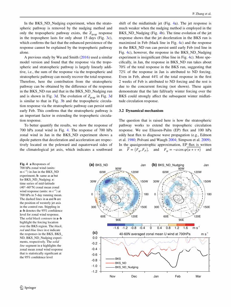
To better quantify the results, we show the response of 700  hPa zonal wind in Fig.  4. The response of 700  hPa zonal wind in Jan in the BKS_ND experiment shows a dipole pattern that deceleration and acceleration are respec-tively located on the poleward and equatorward sides of the climatological jet axis, which indicates a southward

shift of the midlatitude jet (Fig.  4a). The jet response is much weaker when the nudging method is employed in the BKS_ND_Nudging (Fig. 4b). The time evolution of the jet response shows that the jet deceleration in the BKS run is maximized in Feb (black line in Fig. 4c) and the response in the BKS_ND run can persist until early Feb (red line in Fig. 4c), however, the response in the BKS_ND_Nudging experiment is insignificant (blue line in Fig. 4c). More spe-cifically, in Jan, the response in BKS_ND run takes about 70% of the total response in the BKS run, suggesting that 72% of the response in Jan is attributed to ND forcing. Even in Feb, about 44% of the total response in the first 2 weeks of Feb is attributed to ND forcing and the rest is due to the concurrent forcing (not shown). These again demonstrate that the late fall/early winter forcing over the BKS could strongly affect the subsequent winter midlati-tude circulation response.

3.2 Dynamical mechanism

The question that is raised here is how the stratospheric pathway works to extend the tropospheric circulation response. We use Eliassen-Palm (EP) flux and 100  hPa eddy heat flux to diagnose wave propagation (e.g., Edmon et al. 1980; Polvani and Waugh 2004; Simpson et al. 2009). In the quasigeostrophic approximation, EP flux is written as �⃗F =

(F𝜑,FP

), and F� = −a cos�⟨u ∗ v ∗⟩ and

Fig. 4 a Responses of 700 hPa zonal wind (units: m s−1) in Jan in the BKS_ND experiment; b: same as a but for BKS_ND_Nudging; c: time series of mid-latitude (40°–60°N) zonal mean zonal wind response (units: m s−1) at 700 hPa in 5-day running mean. The dashed lines in a and b are the position of westerly jet axis in the control run. Stippling in a–b denotes the 95% confidence level for zonal wind response. The solid black contours in a–b highlight the forcing location over the BKS region. The black, red and blue lines in c indicate the responses in the BKS, BKS_ND, BKS_ND_Nudging experi-ments, respectively. The solid line segment in c highlights the zonal mean zonal wind response that is statistically significant at the 95% confidence level

(a)

(c)

(b)

Prolonged effect of the stratospheric pathway in linking Barents–Kara Sea sea ice variability…

1 3

FP = af cos��

�∗�∗

⟨�⟩P

�, where f is the Coriolis parameter, u

and v are zonal and meridional velocities, � is potential temperature, ⟨⟩ denotes zonal average, superscript * denotes deviation from zonal mean and overbar denotes time aver-age. The EP flux divergence is calculated as

1

a cos𝜑∇ ⋅ �⃗F =

1

a cos𝜑

{1

a cos𝜑

𝜕

𝜕𝜑(F𝜑 cos𝜑) +

𝜕

𝜕PFP

}. The

direction of EP flux indicates the wave propagation and the flux divergence measures the wave forcing on the zonal wind. In addition, the eddy heat flux anomaly can be decomposed into four components: Δ⟨� ∗ T ∗⟩ =�Δ� ∗T

∗

c

�+

�Δ� ∗

cT∗�+

�Δ�

∗T∗�+ Δ⟨� ∗� T ∗�⟩,

where Δ is the difference between perturbation experiment and control run, subscript c denotes CTRL run and prime denotes deviation from time average. The first two terms on the right-hand-side are the linear components, the third term is the nonlinear component and the fourth term is the high-frequency fluctuation component.

Here we focus on the BKS_ND experiment. As the Zpcap shown in Fig. 3b and the zonal mean zonal wind in Figure S3 a, as a result of ND near-surface heating, the stratospheric polar vortex weakens in Dec. This circulation response persists in the stratosphere until early Feb accom-panied by downward migration back to the troposphere and the surface. We choose Dec as the upward propaga-tion phase, which is before the termination of the forcing (Jan 1). The period of Jan 15–Feb 10 is considered as the downward migration phase, since the tropospheric pathway alone can be ignored about 2 weeks after the termination of the forcing (shown in Fig. 3c), and the delayed response persists for about 40 days until early Feb (as can be seen in Figs.  3b, 4c). This downward migration processes can be better seen by the lead-lag correlation of Zpcap at all lev-els with Zpcap at 100 hPa in the difference of BKS_ND run and BKS_ND_Nudging run (Figure S4). As can be seen, the signal in the middle-upper stratosphere leads that in the lower stratosphere and troposphere by about 1 week.

During the upward propagation phase, during Dec in the BKS_ND run, anomalous EP flux is excited mostly over 40°–60°N, associated with increased baroclinicity in this region slightly equatorward of the heating anomaly, and planetary-scale waves propagate into the lower stratosphere (Fig.  5a). The EP flux anomaly and its resulting EP flux convergence, which is dominated by its vertical component related to eddy heat flux, is responsible for the weakening of the stratospheric polar vortex (Fig. 5a). The decomposi-tion of the eddy heat flux at 100 hPa shows that this upward propagating wave response can be mainly attributed to its linear component and both the nonlinear and high-fre-quency components are very small (Fig.  5b). This linear component is due to the linear constructive interference

mechanism where the wave anomaly is largely in phase with the wave climatology and planetary-scale waves can propagate effectively into the stratosphere [see Fig. 10a and also in Garfinkel et al. (2010) and Smith et al. (2010)].

For the later downward migration phase, during Jan 15–Feb 10, the EP flux response is mostly concentrated in the troposphere (Fig.  5c). Compared to the upward propagation phase, there is anomalous poleward propagat-ing EP flux in the midlatitude troposphere, indicating the critical role of eddy momentum flux. The convergence of anomalous EP flux, dominated by eddy momentum flux

(a)

(b)

(c)

Fig. 5 a Response of the EP flux (vector, units: 1015 m3), zonal mean zonal wind (blue contour, contour interval is 0.5  m  s−1 , negative values are dashed) and vertical component of the EP flux divergence (color shading, units: m s−1 day−1) in December in the BK_ND run. The EP flux is multiplied by the square root of 1000/pressure (hPa) to better demonstrate the waves in the stratosphere. b Response of 100 hPa zonal mean eddy heat flux (black) and its decomposition into linear (red), nonlinear (green) and high frequency components (pur-ple) in December in the BKS_ND run (units: K m s−1). c Similar to a but during Jan 15–Feb 10 and the color shading in c is the horizontal component of the EP flux divergence response

P. Zhang et al.

1 3

component, at about 40°–60°N favors the persistence of the midlatitude westerly deceleration in the troposphere. The detailed mechanism of downward migration has been examined extensively in previous studies (e.g., Hartley et al. 1998; Perlwitz and Harnik 2003; Kushner and Polvani 2004; Song and Robinson 2004; Simpson et al. 2009) and is beyond the scope of this study.

3.3 Induced cold winter over central Asia

In addition to the midlatitude jet response, another con-sequence of Arctic sea ice melting is its possible impact on Eurasian cold air outbreaks, but the evidence for this impact is less clear. Some studies attribute the increased mid-latitude extremes in recent years to the declining trend of Arctic sea ice (e.g., Honda et  al. 2009; Petoukhov and Semenov 2010; Francis and Vavrus 2012; Cohen et  al. 2014; Mori et al. 2014; Kug et al. 2015); however, others argue that there is no robust response or, in contrast, fewer extremes to Arctic sea ice loss (Barnes 2013; Hassanzadeh

et al. 2014; Li et al. 2015; McCusker et al. 2016; Sellevold et al. 2016; Sun et al. 2016). Here, we simply document the results from our idealized AGCM experiments. Figure  6 shows the circulation and temperature response in Dec in the BKS_ND run and BKS_ND_Nudging run. As shown in Fig. 6b, there is an induced cold response over central Asia as a result of imposed heating over the BKS region, which resembles that in observations (shown in Fig.  1a). This induced cold anomaly remains robust with other choices of forcing parameters (see Figure S2 b and d for an example with a weaker (1.5 K day−1) and a stronger (4.0 K day−1) forcing magnitude). This cold response is also deep in the vertical column in troposphere (Fig. 6a). However, this cold response becomes weaker in the nudging experiment in which the stratospheric pathway is deactivated (Fig. 6b, d), and this demonstrates that the stratospheric pathway also plays an important role in amplifying the central Asia cold events. Figure 7 is similar to Fig. 6 but for Jan. Even though the forcing is switched off, a cold response can still be seen over central Asia in the BKS_ND experiment. However,

(a) (b)

(c) (d)

Fig. 6 a 40°–50°N averaged longitude-pressure cross-section of tem-perature (color shading) and geopotential height (contour, contour interval is 4 gpm, negative values are dashed) responses in Decem-ber in the BKS_ND run. b Response of temperature (color shading, units: K) and wind (vector, units: m  s−1) at the lowest model level (sigma = 0.947) in January in the BKS_ND run. c and d Same as a

and b but for the BKS_ND_Nudging experiment. The white symbol ‘A’ in b highlights the anticyclonic anomalies. Stippling denotes the 95% confidence level for temperature. Only the surface wind response at the 95% confidence level is shown in b and d. The solid black con-tour in b, d highlights the forcing location

Prolonged effect of the stratospheric pathway in linking Barents–Kara Sea sea ice variability…

1 3

the cold response almost disappears near the surface in the BKS_ND_Nudging experiment and the lower stratosphere upper troposphere and the surface appears de-coupled.

This induced cold anomaly over central Asia is mainly a result of the circulation response. A negative Arctic Oscil-lation (AO)-like pattern is found over the NH extra-tropics (figure not shown) and an anomalous deep warm high ridge is found near the Ural Mountains (35°–65°E) and occu-pies the entire troposphere (Fig. 6a), which is in agreement with observations and comprehensive model experiments (e.g., Mori et al. 2014; Cohen et al. 2014; Overland et al. 2015). The accompanied anticyclonic circulation anomaly, even though weak in magnitude, is found on the southern side of BKS forcing (highlighted by the white symbol ‘A’ in Fig. 6b), which is consistent with observations and com-prehensive model experiments (see Fig.  1 in Mori et  al. 2014). The high ridge near the Ural Mountains and the associated northerly wind to the east leads to more cold air advection from the Arctic region to central Asia (Fig. 6b). The high ridge and the northerly flow are weaker in the nudging experiment (Fig.  6c, d), which is responsible for the weaker cold anomaly over central Asia. Similar circu-lation response can be seen in Jan (Fig.  7). These results

suggest that the existence of the stratospheric pathway, i.e., the dynamical coupling between the troposphere and stratosphere, acts to enhance the intensity and prolong the duration of midlatitude ridge/trough, resulting in enhanced surface cooling response over central Asia.

3.4 Sensitivity to geographical location of the forcing

Recent studies suggested that the sea ice loss in different regions over the Arctic might have different impacts on the midlatitude circulation (Sun et al. 2015; Koenigk et al. 2016; Pedersen et  al. 2016). Therefore, in addition to the BKS experiments, here we also investigate the sensitiv-ity of the midlatitude circulation response to geographi-cal location of the forcing, more specifically over the East Siberian Sea (ESS) and Greenland (GLD) (see Fig. 2a), by using the idealized model.

Figure  8a is similar to Fig.  3b but for the ESS_ND experiments, in which the forcing is imposed during ND over the ESS region. The Zpcap also increases in the tropo-sphere and lower stratosphere but the intensity is weaker, especially in the stratosphere, and the persistence is shorter than that in the BKS_ND run. In the nudging experiment

(a) (b)

(c) (d)

Fig. 7 Same as Fig. 6 but for January

P. Zhang et al.

1 3

for ESS_ND forcing (Fig. 8c), the tropospheric pathway is comparable to that in BKS_ND forcing experiment. How-ever, the stratospheric response and downward migration is nearly absent after the termination of the forcing (Fig. 8e). In the GLD_ND experiment, the Zpcap response is very weak both in the troposphere and stratosphere (Fig.  8b) with both weak tropospheric and stratospheric pathways (Fig. 8d, f).

Figure 9 compares the midlatitude low-level jet response in the BKS_ND, ESS_ND and GLD_ND experiments. In the ESS_ND run, the midlatitude low-level jet response is comparable to that in the BKS_ND run in Dec, but is not robust beyond early Jan. The ESS_ND forcing induced cir-culation is mostly due to the tropospheric adjustment itself with a minor contribution from stratosphere-troposphere coupling (Figure S5). The lack of prolonged stratospheric downward migration effect by the ESS_ND forcing likely contributes to the short persistence of the tropospheric jet response. The jet response in GLD_ND run is very weak

and is insignificant, which is due to the weak response via both the tropospheric and stratospheric pathway.

Compared to the BKS_ND run, although the structure and intensity of the forcing is exactly same in the ESS_ND run and GLD_ND run, the circulation responses are differ-ent in those experiments, which imply that the midlatitude

gpm

(a) (b)

(c) (d)

(e) (f)

Fig. 8 a, c and e same as Fig. 3b–d but for forcing centered at East Siberian Sea (ESS); b, d and f same as Fig. 3b–d but for forcing centered at Greenland (GLD)

Fig. 9 Same as Fig. 4c but for ESS_ND run (green) and GLD_ND run (purple). The red line is BKS_ND run, same as the red line in Fig. 4c

Prolonged effect of the stratospheric pathway in linking Barents–Kara Sea sea ice variability…

1 3

response and troposphere–stratosphere coupling are sensi-tive to the geographical location of the forcing.

To better understand the stratosphere–troposphere cou-pling to geographical location for the forcing, Fig.  10 shows the response of zonal wave-1 and wave-2 geopoten-tial height. It is found that the BKS region is close to the climatological ridge of both wave-1 and wave-2 and thus the BKS forcing excites anomalous ridge in phase with the climatology. This planetary wave response in-phase with the control state is known as linear constructive inter-ference and effectively excites the vertical wave propa-gation into stratosphere and a weaker polar vortex (see Sect. 3.2 Smith et al. 2010). The BKS_ND forcing induced wave-1 and wave-2 responses are consistent with previous

observation and comprehensive model results (e.g., Kim et al. 2014; Mori et al. 2014; Sun et al. 2015). On the con-trary, the excited wave-1 and wave-2 anomalies in ESS_ND (Fig.  10b, e) and wave-1 anomalies in GLD_ND experi-ments (Fig. 10c) are mostly out-of-phase with the control state. Although the wave-2 anomalies in GLD_ND experi-ment are in-phase with the control state (Fig. 10f), its con-tribution is much smaller than that of the wave-1 and thus the total response in GLD_ND experiment is still linear deconstructive. This linear deconstructive interference in the troposphere-stratosphere coupling leads to a slightly enhanced polar vortex over high latitudes (Figure S3b, c). In view of Zpcap, it should be noted that the geopotential height is a vertically-integrated quantity and therefore,

(a) (b) (c)

(d) (e) (f)

Fig. 10 45°–70°N averaged zonal wave-1 geopotential height (units: gpm, contour interval is 16 gpm) in the control run (contour, nega-tive dashed), wave-1 response in the BKS_ND run (a), ESS_ND run

(b) and GLD_ND run (c) (color shading) and wave-2 response in the BKS_ND run (d), ESS_ND run (e) and GLD_ND run (f) (color shading) in Dec

P. Zhang et al.

1 3

surface anomalies due to the imposed heating could affect the upper levels. However, the dynamical linear decon-structive interference acts in an opposite manner, partly offsets the Zpcap increase due to the surface temperature increase and leads to weaker Zpcap responses in those two experiments compared to that in BKS_ND run (Fig.  8). Thus, the resulting weaker responses via the stratospheric pathway in ESS_ND and GLD_ND experiments account for the short-lived and weaker responses in the midlatitude circulation (Figs. 8, 9). These results suggest that the BKS region is the most effective in influencing the midlatitude circulation through more active stratospheric pathway than other regions over the Arctic.

4 Conclusion and discussion

In this study we investigate the observed lead-lag correla-tion between the early winter BKS sea ice variability and the later winter midlatitude circulation response using a set of idealized AGCM experiments. First of all, the experi-ment results show that the idealized dry model is able to reproduce the persistent winter circulation response dur-ing Jan–Feb with an imposed near-surface heating dur-ing Nov–Dec. Then by applying a nudging method in the stratosphere and an explicit separation of the tropospheric and stratospheric pathway, it is found that the prolonged midlatitude circulation response is largely due to the strato-spheric pathway and the long time scale in the stratosphere. Second, the dynamic diagnostic results show that the stratospheric pathway works in two phases: the first phase involves upward propagation of planetary-scale waves due to linear constructive interference and the weakening of the stratospheric polar vortex; the second phase involves downward migration from the stratosphere to the tropo-sphere and the surface. This downward migration largely amplifies and extends the low-level jet deceleration. Third, as a result of the imposed heating over the BKS region, an induced cold anomaly is simulated over central Asia, which resembles the feature seen in observations. It is found that the stratospheric pathway also acts to amplify and extend the cold events over central Asia. Above results qualita-tively remain robust when varying the forcing parameters. Finally, further experiments show that the midlatitude cir-culation response is sensitive to the geographical location of the forcing. The BKS region is found the most effective in influencing the midlatitude circulation response than other regions over the Arctic.

The results found in this idealized model setup are largely in agreement with previous studies that suggest an important role of the stratospheric pathway in linking the Arctic sea ice with the midlatitude circulation (e.g., Kim et  al. 2014; Sun et  al. 2015; Nakamura et  al. 2016; Yang

et al. 2016). In contrast with similar studies, we explicitly separate the tropospheric and stratospheric pathway and unequivocally attribute the prolonged midlatitude circu-lation response to the stratospheric pathway and its long time scale. We plan to extend our work to state-of-the-art AGCM and realistic variability of Arctic sea ice to better quantify the lead-lag effect and the role of the stratospheric pathway in future study. This prolonged effect of the strato-spheric pathway may be helpful in better understanding and predicting the midlatitude winter conditions (Scaife et  al. 2014).

Acknowledgements The authors thank Dr. Linjiong Zhou at GFDL for model stability testing and Dr. Yueyue Yu at Florida State Univer-sity for discussion. PZ and YW are supported by the U.S. National Science Foundation (NSF) Climate and Large-Scale Dynamics pro-gram under Grant AGS-1406962 and a start-up fund from the Depart-ment of Earth, Atmospheric, and Planetary Sciences at Purdue Uni-versity. KLS is funded by the NSF Office of Polar Programs, Arctic Research Opportunities, PLR-1603350.

References

Baldwin MP, Stephenson DB, Thompson DWJ, Dunkerton TJ, Charlton AJ, O’Neill A (2003) Stratospheric memory and skill of extended-range weather forecasts. Science 301:636–640. doi:10.1126/science.1087143

Barnes EA (2013) Revisiting the evidence linking Arctic amplifi-cation to extreme weather in midlatitudes. Geophys Res Lett 40(17):4734–4739. doi:10.1002/grl.50880

Barnes EA, Screen JA (2015) The impact of Arctic warming on the midlatitude jet-stream: Can it? Has it? Will it? Wiley Interdiscip Rev Clim Change 6(3):277–286. doi:10.1002/wcc.337

Butler A, Thompson D, Heikes R (2010) The steady-state atmos-pheric circulation response to climate change–like thermal forc-ings in a simple general circulation model. J Clim 23:3474–3496

Cavalieri DJ, Parkinson CL, Gloersen P, Zwally HJ (1996) Sea ice concentrations from Nimbus-7 SMMR and DMSP SSM/I-SSMIS passive microwave data. National Snow and Ice Data Center. Boulder

Cohen J., Screen JA, Furtado JC et al (2014) Recent Arctic amplifica-tion and extreme mid-latitude weather. Nat Geosci 7(9):627–637. doi:10.1038/ngeo2234

Dee DP et al (2011) The ERA-Interim reanalysis: configuration and performance of the data assimilation system. Q J R Meteorolog Soc 137(656):553–597. doi:10.1002/qj.828

Deser C, Magnusdottir G, Saravanan R, Phillips A (2004) The Effects of North Atlantic SST and sea ice anomalies on the winter circulation in CCM3. Part II: direct and indi-rect components of the response. J Clim 17(5):877–889. doi:10.1175/1520-0442(2004)017<0877:TEONAS>2.0.CO;2

Edmon HJ, Hoskins BJ, McIntyre ME (1980) Eliassen-Palm cross sections for the troposphere. J Atmos Sci 37(12):2600–2616. doi:10.1175/1520-0469(1980)037<2600:EPCSFT>2.0.CO;2

Francis JA, Vavrus SJ (2012) Evidence linking Arctic amplifica-tion to extreme weather in mid-latitudes. Geophys Res Lett 39(6):L06801. doi:10.1029/2012GL051000

Garfinkel CI, Hartmann DL, Sassi F (2010) Tropospheric precursors of anomalous northern hemisphere stratospheric polar vortices. J Clim 23(12):3282–3299. doi:10.1175/2010JCLI3010.1

Prolonged effect of the stratospheric pathway in linking Barents–Kara Sea sea ice variability…

1 3

Hartley DE, Villarin JT, Black RX, Davis CA (1998) A new perspec-tive on the dynamical link between the stratosphere and tropo-sphere. Nature 391(6666):471–474

Hassanzadeh P, Kuang Z (2015) Blocking variability: Arctic amplifi-cation versus Arctic oscillation. Geophys Res Lett. doi:10.1002/2015GL065923(2015GL065923)

Hassanzadeh P, Kuang Z, Farrell BF (2014) Responses of midlatitude blocks and wave amplitude to changes in the meridional tem-perature gradient in an idealized dry GCM. Geophys Res Lett 41(14):5223–5232. doi:10.1002/2014GL060764

Held IM, Suarez MJ (1994) A proposal for the intercompari-son of the dynamical cores of atmospheric general circu-lation models. Bull Am Meteorol Soc 75(10):1825–1830. doi:10.1175/1520-0477(1994)075<1825:APFTIO>2.0.CO;2

Honda M, Inoue J, Yamane S (2009) Influence of low Arctic sea ice minima on anomalously cold Eurasian winters. Geophys Res Lett 36(8):L08707. doi:10.1029/2008GL037079

Jaiser R, Dethloff K, Handorf D (2013) Stratospheric response to Arctic sea ice retreat and associated planetary wave propagation changes. Tellus A 65:19375. doi:10.3402/tellusa.v65i0.19375

Kim B-M, Son S-W, Min S-K, Jeong J-H, Kim S-J, Zhang X, Shim T, Yoon J-H (2014) Weakening of the stratospheric polar vortex by Arctic sea-ice loss. Nat Commun. doi:10.1038/ncomms5646

Koenigk T, Caian M, Nikulin G, Schimanke S (2016) Regional Arc-tic sea ice variations as predictor for winter climate conditions. Clim Dynam 46(1):317–337. doi:10.1007/s00382-015-2586-1

Kug J-S, Jeong J-H, Jang Y-S, Kim B-M, Folland C K, Min S-K, Son S-W (2015) Two distinct influences of Arctic warming on cold winters over North America and East Asia. Nat Geosci 8(10):759–762. doi:10.1038/ngeo2517

Kushner PJ, Polvani LM (2004) Stratosphere–troposphere cou-pling in a relatively simple AGCM: the role of eddies. J Clim 17(3):629–639

Kushner PJ, Polvani LM (2006) Stratosphere–troposphere coupling in a relatively simple AGCM: impact of the seasonal cycle. J Clim 19(21):5721–5727. doi:10.1175/JCLI4007.1

Lee M-Y, Hong C-C, Hsu H-H (2015) Compounding effects of warm sea surface temperature and reduced sea ice on the extreme cir-culation over the extratropical North Pacific and North Amer-ica during the 2013–2014 boreal winter. Geophys Res Lett 42(5):2014GL062956. doi:10.1002/2014GL062956

Li C, Stevens B, Marotzke J (2015) Eurasian winter cool-ing in the warming hiatus of 1998–2012. Geophys Res Lett 42(19):2015GL065327. doi:10.1002/2015GL065327

McCusker KE, Fyfe JC, Sigmond M (2016) Twenty-five winters of unexpected Eurasian cooling unlikely due to Arctic sea-ice loss. Nature Geosci 9(11):838–842

Mori M, Watanabe M, Shiogama H, Inoue J, Kimoto M (2014) Robust Arctic sea-ice influence on the frequent Eurasian cold winters in past decades. Nat Geosci 7(12):869–873. doi:10.1038/ngeo2277

Nakamura T, Yamazaki K, Iwamoto K, Honda M, Miyoshi Y, Ogawa Y, Tomikawa Y, Ukita J (2016) The stratospheric pathway for Arctic impacts on midlatitude climate. Geophys Res Lett. doi:10.1002/2016GL068330(2016GL068330)

Overland J, Francis JA, Hall R, Hanna E, Kim S-J, Vihma T (2015) The melting Arctic and midlatitude Weather patterns: are they connected? J Clim 28(20):7917–7932. doi:10.1175/JCLI-D-14-00822.1

Pedersen RA, Cvijanovic I, Langen PL, Vinther BM (2016) The impact of regional Arctic Sea ice loss on atmospheric circulation and the NAO. J Clim 29:889–902

Perlwitz J, Harnik N (2003) Observational evidence of a stratospheric influence on the troposphere by planetary wave reflection. J Clim 16:3011–3026

Petoukhov V, Semenov VA (2010) A link between reduced Barents–Kara sea ice and cold winter extremes over northern continents. J Geophys Res Atmos 115(D21):D21111. doi:10.1029/2009JD013568

Polvani LM, Kushner PJ (2002) Tropospheric response to strato-spheric perturbations in a relatively simple general circulation model. Geophys Res Lett 29(7):18-11-18-14. doi:10.1029/2001GL014284

Polvani LM, Waugh DW (2004) Upward wave activity flux as a pre-cursor to extreme stratospheric events and subsequent anoma-lous surface weather regimes. J Clim 17(18):3548–3554. doi:10.1175/1520-0442(2004)017<3548:UWAFAA>2.0.CO;2

Reynolds RW, Rayner NA, Smith TM, Stokes DC, Wang W (2002) An improved in situ and satellite SST analysis for climate. J Clim 15(13):1609–1625. doi:10.1175/1520-0442(2002)015<1609:AIISAS>2.0.CO;2

Scaife AA et  al (2014) Skillful long-range prediction of Euro-pean and North American winters. Geophys Res Lett 41(7):2014GL059637. doi:10.1002/2014GL059637

Screen AJ, Deser C, Sun L (2015) Projected changes in regional cli-mate extremes arising from Arctic sea ice loss. Environ Res Lett 10(8):084006

Sellevold R, Sobolowski S, Li C (2016) Investigating possible Arc-tic–midlatitude teleconnections in a linear framework. J Clim 29(20):7329–7343

Simpson IR, Blackburn M, Haigh JD (2009) The role of eddies in driving the tropospheric response to stratospheric heating per-turbations. J Atmos Sci 66(5):1347–1365. doi:10.1175/2008JAS2758.1

Simpson IR, Hitchcock P, Shepherd TG, Scinocca JF (2011) Strato-spheric variability and tropospheric annular-mode timescales. Geophys Res Lett 38(20):L20806. doi:10.1029/2011GL049304

Smith KL, Fletche CG, Kushner PJ (2010) The role of linear interfer-ence in the annular mode response to extratropical surface forc-ing. J Clim 23(22):6036–6050. doi:10.1175/2010JCLI3606.1

Song Y, Robinsion W (2004) Dynamical mechanisms for stratospheric influences on the troposphere. J Atmos Sci 61(14):1711–1725

Sun L, Deser C, Tomas RA (2015) Mechanisms of stratospheric and tropospheric circulation response to projected arctic sea ice loss. J Clim 28(19):7824–7845. doi:10.1175/JCLI-D-15-0169.1

Sun L, Perlwitz J, Hoerling M (2016) What caused the recent “Warm Arctic, Cold Continents” trend pattern in winter temperatures? Geophys Res Lett. doi:10.1002/2016GL069024(2016GL069024)

Vihma T (2014) Effects of Arctic sea ice decline on weather and cli-mate: a review. Surv Geophys 35(5):1175–1214. doi:10.1007/s10712-014-9284-0

Wu Y, Smith KL (2016) Response of northern hemisphere midlatitude circulation to arctic amplification in a simple atmospheric gen-eral circulation model. J Clim. doi:10.1175/JCLI-D-15-0602.1

Wu Q, Zhang X (2010) Observed forcing-feedback processes between Northern Hemisphere atmospheric circulation and Arctic sea ice coverage. J Geophys Res Atmos 115(D14):D14119. doi:10.1029/2009JD013574

Yang X-Y, Yuan X, Ting M (2016) Dynamical link between the Bar-ents–Kara Sea ice and the Arctic oscillation. J Clim 29:5103–5122. doi: 10.1175/JCLI-D-15-0669.1