Prologue Prologue ––

Perspective, Perspective, Premises and Presentation PlanPremises and Presentation Plan

--

A look at data assimilation issues from a data A look at data assimilation issues from a data perspective instead of an assimilation one.perspective instead of an assimilation one.

--

4D4D--Var context assumed: Var context assumed: Mesoscale focus Mesoscale focus Fewer valid meteorological Fewer valid meteorological approximations + approximations + Limited datasets Limited datasets Need to look at the time Need to look at the time evolution of fields to retrieve the many unobserved variables.evolution of fields to retrieve the many unobserved variables.

--

Presentation focus is on explaining paradigm Presentation focus is on explaining paradigm and showing results; light on methods/details.and showing results; light on methods/details.

Blue: 4-min assimilationPurple: 8-min assimilationIf the well

observed storm intensity is so sensitive to low level moisture...

… then why can’t we retrieve low-

level moisture by assimilating radar data?

(Td ≈

20°C)(Td ≈

21.5°C)

Source: Presentation by N.A. Crook et al., 2004: Assimilation of

radar observations of a supercell

storm using 4DVar…. 22nd

Conf. on Severe and Local Storms.

Conditions for a SuccessfulConditions for a Successful Data AssimilationData Assimilation

1)1)

The difference between the expected The difference between the expected atmospheric state atmospheric state xx’’

and the true atmospheric and the true atmospheric

state state xx

results in a measurable difference results in a measurable difference between the expected observations between the expected observations yy’’

and the and the

true observations true observations yy..2)2)

Given Given xx’’

and and xx, a model can reproduce the , a model can reproduce the

associated observations associated observations yy’’

and and yy..3)3)

The data assimilation system can use The data assimilation system can use yy’’

and and yy

to change the model state from to change the model state from xx’’

to to xx..Something Something ““failedfailed””

in Crook et al. But what?in Crook et al. But what?

A Pathway to FailureA Pathway to FailureRealityModel assimilating radar reflectivity

Time T zx

What if the model is too dry?

A Pathway to FailureA Pathway to FailureReality

Time T zx

+1 min+2 min+3 min+4 min

Model assimilating radar reflectivity

A Pathway to FailureA Pathway to Failure

In this case, only a data assimilation process exceeding In this case, only a data assimilation process exceeding 20 minutes would constrain surface moisture data.20 minutes would constrain surface moisture data.

Reality

Time T zx

Constrained by observationsUnconstrained by observations(yet important in determining the storm’s future)

4-min data assimilation

Model assimilating radar reflectivity

Arising QuestionsArising Questions••

What type of initialization errors can be detected What type of initialization errors can be detected by observing which parameters over what by observing which parameters over what duration? Focus is on the presence of a signal, duration? Focus is on the presence of a signal, and not on the specifics of its assimilation.and not on the specifics of its assimilation.

••

What existing observing What existing observing system(ssystem(s) ) provide(sprovide(s) ) the most information for mesoscale forecasting? the most information for mesoscale forecasting? Where should assimilation efforts be focused on Where should assimilation efforts be focused on (instrument and window duration(instrument and window duration--wise)?wise)?

••

What about future observing systems?What about future observing systems?

A systematic study is needed (and doable).A systematic study is needed (and doable).

For How Long Should What For How Long Should What Data Be Assimilated for Data Be Assimilated for

Mesoscale Forecasting and Mesoscale Forecasting and Why?Why?

FrFrééddééric Fabryric FabryMcGill University, Montreal, CanadaMcGill University, Montreal, Canada

With the help and counsel of: Kay, Chris, Rich, Yongsheng, Wei, Michael, Morris, Joseph, Bill, David, Peggy, Don, Barry,

Jenny Sun, Eunha

Lim, Qingnong

Xiao, and Sherrie Fredrick

Questions of Interest, Part IQuestions of Interest, Part I

••

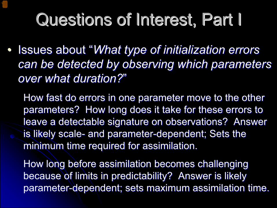
Issues about Issues about ““What type of initialization errors What type of initialization errors can be detected by observing which parameters can be detected by observing which parameters over what duration?over what duration?””How fast do errors in one parameter move to the other How fast do errors in one parameter move to the other parameters? How long does it take for these errors to parameters? How long does it take for these errors to leave a detectable signature on observations? Answer leave a detectable signature on observations? Answer is likely scaleis likely scale--

and parameterand parameter--dependent;dependent;

Sets the Sets the

minimum time required for assimilation.minimum time required for assimilation.

How long before assimilation becomes challenging How long before assimilation becomes challenging because of limits in predictability? Answer is likely because of limits in predictability? Answer is likely parameterparameter--dependent; sets maximum assimilation time.dependent; sets maximum assimilation time.

Assimilation and PredictabilityAssimilation and Predictability

Model state:

Truth:

Towards truth:

(1): Linear region:(1): Linear region:

(2): Nonlinear region:(2): Nonlinear region:

(3): (3): ““ContradictoryContradictory””

region: Adjusting region: Adjusting xx(initial(initial) towards ) towards xx++kk∆∆xx(initial(initial) worsens the fit to ) worsens the fit to M(M(xx++∆∆xx) ) Assimilation Assimilation of these (perfect) data will of these (perfect) data will worsenworsen the fit with the truth.the fit with the truth.

( ) ( ) ( ) xxxxx Δ∂∂+≈Δ+ MMM( ) ( ) ( ) ( )[ ]xxxxxx MMkMkM −Δ+≈−Δ+

( ) ( ) ( ) ( )[ ]xxxxxx MMkMkM −Δ+≠−Δ+

Questions of Interest, Part IIQuestions of Interest, Part II••

Issues about Issues about ““What existing, planned, or What existing, planned, or unplanned observing unplanned observing system(ssystem(s) ) provide(sprovide(s) the ) the most information for mesoscale forecasting?most information for mesoscale forecasting?””How much do typical errors in each parameter affect How much do typical errors in each parameter affect forecast quality? Could significant gains in forecast forecast quality? Could significant gains in forecast accuracy be made by focusing on a few parameters? accuracy be made by focusing on a few parameters? Of interest for assimilation and for instrument design.Of interest for assimilation and for instrument design.

Which instruments or technologies provide the most Which instruments or technologies provide the most information? Answer depends on information? Answer depends on variable(svariable(s) targeted ) targeted by instrument because of all the aforementioned issues, by instrument because of all the aforementioned issues, data coverage, measurement accuracy, and strength of data coverage, measurement accuracy, and strength of link between the quantity observed and the variables.link between the quantity observed and the variables.

Overall Approach:Overall Approach: Identical Twins ExperimentIdentical Twins Experiment

••

““TruthTruth””: Simulate a series of plausible convective events : Simulate a series of plausible convective events (12(12--hr long control runs);hr long control runs);

••

Error growth experimentError growth experiment: Perturb initial conditions by a : Perturb initial conditions by a plausible plausible ““errorerror””), and run a ), and run a ““forecastforecast””;;

••

Check the magnitude of the resulting forecast error as a Check the magnitude of the resulting forecast error as a function of the type of errors in the initial conditions; function of the type of errors in the initial conditions;

••

Study the properties of the transfer of errors from one Study the properties of the transfer of errors from one parameter to the next; focus on magnitude, predictability;parameter to the next; focus on magnitude, predictability;

••

Evaluate the ability of different sensors of detecting early Evaluate the ability of different sensors of detecting early signs of the forecast going astray.signs of the forecast going astray.

In Detail:In Detail: 1) Model and Domain Used1) Model and Domain Used

••

WRF v. WRF v. ßß2.22.2

••

1600 x 1600 km 1600 x 1600 km domaindomain

••

4 km resolution, 4 km resolution, 28 levels28 levels

••

Thompson et al. Thompson et al. micromicrophysics, physics, RRTM & RRTM & DudhiaDudhia

radiation, Noah radiation, Noah land surface, land surface, YSU PBLYSU PBL……

Terrain height (m)

In Detail:In Detail: 2) The Model Runs2) The Model Runs

Sixteen 12Sixteen 12--hr runs; one every 9 hrs for a 6hr runs; one every 9 hrs for a 6--day period (10day period (10--16 June 2002)16 June 2002)

T T ––

3 hrs3 hrs TT

Initialized with Initialized with ETA analysisETA analysis

Warm-upT + 12 hrsT + 12 hrs

Control run (“truth”)

Perturbed runs

Perturbed fields:Perturbed fields:•• LowLow--levellevel

HumidityHumidity

•• MidMid--levellevel

TemperatureTemperature•• HiHi--levellevel

WindsWinds

•• CondensatesCondensates•• Soil moistureSoil moisture

In Detail:In Detail: 3) The Perturbations3) The Perturbations

Wavelength (km)101001000

Ene

rgy

(rel

ativ

e un

its)

1

10

100

1000

-4σ 4σ0 2σ-2σ

In Detail:In Detail: 3) The Perturbations3) The Perturbations

High-level perturbations: from η

= .15 to η

= .5

Mid-level perturbations: from η

= .5 to η

= .85

Low-level perturbations: from η

= .825 to η

= 1

Wavelength (km)101001000

Ene

rgy

(rel

ativ

e un

its)

1

10

100

1000

-4σ 4σ0 2σ-2σ

CondensatesCondensatesLowLow--level humiditylevel humidity

Condensatesσ

= 40%

Low-levelhumidity; σ

= 7%

Model levels

In Detail:In Detail: 3) The Perturbations3) The Perturbations

Soil moisture before (left) and after (right) Soil moisture before (left) and after (right) ±±25% perturbation25% perturbation

0% 100%50%

In Detail:In Detail: 4) The Data Obtained4) The Data Obtained

Sixteen 12Sixteen 12--hr runs; one every 9 hrs for a 6hr runs; one every 9 hrs for a 6--day period (10day period (10--16 June 2002)16 June 2002)

T T ––

3 hrs3 hrs

Initialized with Initialized with ETA analysisETA analysis

Warm-up

Perturbed runs

••

Model outputs every 15 min up to T+1Model outputs every 15 min up to T+1½½; ; more model outputs on the hour up to T+12.more model outputs on the hour up to T+12.““ObservationsObservations””

are evaluated up to T+3.are evaluated up to T+3.

Control run (“truth”)

TT T+1T+1½½ T+3T+3 T+12T+12

In Detail:In Detail: 4) The Data Obtained4) The Data Obtained

Sixteen 12Sixteen 12--hr runs; one every 9 hrs for a 6hr runs; one every 9 hrs for a 6--day period (10day period (10--16 June 2002)16 June 2002)

T T ––

3 hrs3 hrs

Initialized with Initialized with ETA analysisETA analysis

Warm-up

Perturbed runs

Control run (“truth”)

TT T+1T+1½½ T+3T+3 T+12T+12

Runs with Runs with ⅛⅛

of the perturbationof the perturbation

••

Partially perturbed run up to T+3 allows us Partially perturbed run up to T+3 allows us to test for the linearity of the forecast errors to test for the linearity of the forecast errors and of the change in the measurements.and of the change in the measurements.

The Simulated WeatherThe Simulated Weather

Right: Rainfall Right: Rainfall accumulation over the accumulation over the 16 control runs.16 control runs.

Despite the limited Despite the limited period, much weather period, much weather occurred with different occurred with different types of forcing types of forcing mechanisms. Hopefully mechanisms. Hopefully the results will be the results will be representative.representative.

Forecast Errors: Analysis ApproachForecast Errors: Analysis Approach

How do we compare errors in winds, temperature, How do we compare errors in winds, temperature, humidity, and precipitation?humidity, and precipitation?

An approach: Use as inspiration An approach: Use as inspiration TalagrandTalagrand’’ss

energy energy difference of perturbations (difference of perturbations (∆∆E) per unit mass:E) per unit mass:

∆∆E = E = ½½

∫∫

[[∆∆uu22

+ + ∆∆vv22

+ + ccpp

//TTrefref

∆∆TT2 2 + + RRTTrefref

((∆∆p/pp/prefref

))22]dV]dVKinetic EKinetic E

Thermal E Pressure EThermal E Pressure E

Vapor: LH = L Vapor: LH = L ∆∆rrvv

= = ccp p ((LL∆∆rrvv

//ccpp

) = c) = cpp

∆∆TTlatentlatent

∆∆EEvv = c= cpp//TTrefref ∆∆TTlatentlatent22 = L= L22/(/(ccppTTrefref) ) ∆∆rrvv

22

Condensates:Condensates:

∆∆EEcc

= = ∆∆PE+PE+∆∆KE KE ≈≈

∆∆PE = PE = ∑∑ghgh

∆∆rr

r,s,gr,s,g

Forecast Errors: Analysis ApproachForecast Errors: Analysis Approach

How do we compare errors in winds, temperature, How do we compare errors in winds, temperature, humidity, and precipitation? Energy differences:humidity, and precipitation? Energy differences:

[wind] KED = [wind] KED = ½½

((∆∆uu22

+ + ∆∆vv22))

++

[temperature] TED = [temperature] TED = ½½

∑∑

ccpp

//TTrefref

∆∆TT22

++

[pressure] PED = [pressure] PED = ½½

∑∑

RRTTrefref

((∆∆p/pp/prefref

))22

++

[vapor] LED = L[vapor] LED = L22/(/(ccpp

TTrefref

) ) ∆∆rrvv

22

++

[condensates] CED = |[condensates] CED = |ghgh

∆∆rrr,s,gr,s,g

||

==

[sum] SED = KED + TED + LED + CED[sum] SED = KED + TED + LED + CED

Forecast Errors: Main ResultsForecast Errors: Main ResultsMidMid--level humidity level humidity uncertainty dominatesuncertainty dominates

For long mesoscale For long mesoscale forecasts: all other forecasts: all other errors are comparableerrors are comparable

For short mesoscale For short mesoscale forecasts: 4 groups of forecasts: 4 groups of different magnitudesdifferent magnitudes

Assimilation Assimilation priorities should differ priorities should differ for different forecasts for different forecasts

Forecast Errors: Other ResultsForecast Errors: Other Results••

Day vs. night runs: Day vs. night runs:

some changes in the some changes in the overall magnitude overall magnitude (daytime differences (daytime differences are larger), but are larger), but minorminor

changes in the ranking changes in the ranking between perturbations;between perturbations;

••

Significant runSignificant run--toto--run run differences, with differences, with forecast error growth forecast error growth being correlated with being correlated with mean rainfall rate.mean rainfall rate.

Forecast Errors: ResultsForecast Errors: Results

The origin of the perturbations is mostly forgotten by T = 3 houThe origin of the perturbations is mostly forgotten by T = 3 hours: rs: Each term is a nearEach term is a near--constant fraction of SED.constant fraction of SED.

Other measures of forecast mismatch would give similar results.Other measures of forecast mismatch would give similar results.

Perturbations in: Winds Temperature Humidity SoilPerturbations in: Winds Temperature Humidity Soil

KineticKinetic

ThermalThermal

LatentLatent

PotentialPotential((precipprecip.).)

Forecast Errors: ResultsForecast Errors: Results

By T = 15 min, perturbation redistribution is By T = 15 min, perturbation redistribution is generally well underway generally well underway Easier detection.Easier detection.Exceptions: lowExceptions: low--level humidity, condensates level humidity, condensates perturbations that undergo slow starts.perturbations that undergo slow starts.

KineticKinetic

ThermalThermal

LatentLatent

Potential (Potential (precipprecip.).)

2 hrs

Forecast Errors: Forecast Errors: Partial ConclusionsPartial Conclusions

••

MidMid--level (centered on 700 level (centered on 700 mbmb) moisture ) moisture uncertainty seems to have the largest impact on uncertainty seems to have the largest impact on forecasts; other uncertainties have lesser forecasts; other uncertainties have lesser impacts, but these vary with forecast timescale.impacts, but these vary with forecast timescale.

••

Most perturbations, especially the ones growing Most perturbations, especially the ones growing fast, get transferred rapidly to other variables.fast, get transferred rapidly to other variables.

If the assimilation is long enough, most types of If the assimilation is long enough, most types of instruments have the opportunity to get a signal instruments have the opportunity to get a signal resulting from the perturbations.resulting from the perturbations.But how useful a signal?But how useful a signal?

Linearity of PerturbationsLinearity of Perturbations

Many data assimilation systems work best if the Many data assimilation systems work best if the perturbations to the model state are linear:perturbations to the model state are linear:

Or:Or:

Model state:

Truth:

Towards truth:

( ) ( ) ( ) ( )[ ]oooooo xxxxxx MMkMkM −Δ+≈−Δ+

( ) ( ) ( ) oxooo xxxxxoΔ∂∂+≈Δ+ MMM

Linearity of PerturbationsLinearity of Perturbations

Linear perturb.: Linear perturb.:

Or:Or:

We can use this property to define a nonlinearity We can use this property to define a nonlinearity index NLI for each variable index NLI for each variable VV::

( )( ) ( )[ ] ( ) ( )[ ]

( ) ( )∑∑

−Δ+

−Δ+−−Δ+=Δ

zyx

zyx

k

kktNLI

,,

,,,,00

0000

xVxxV

xVxxVxVxxVxV

( ) ( ) xx

xxx0x

00 Δ⎟⎠⎞

⎜⎝⎛∂∂

+≈Δ+MMM

( ) ( ) ( ) ( )[ ]0000 xxxxxx MMkMkM −Δ+≈−Δ+

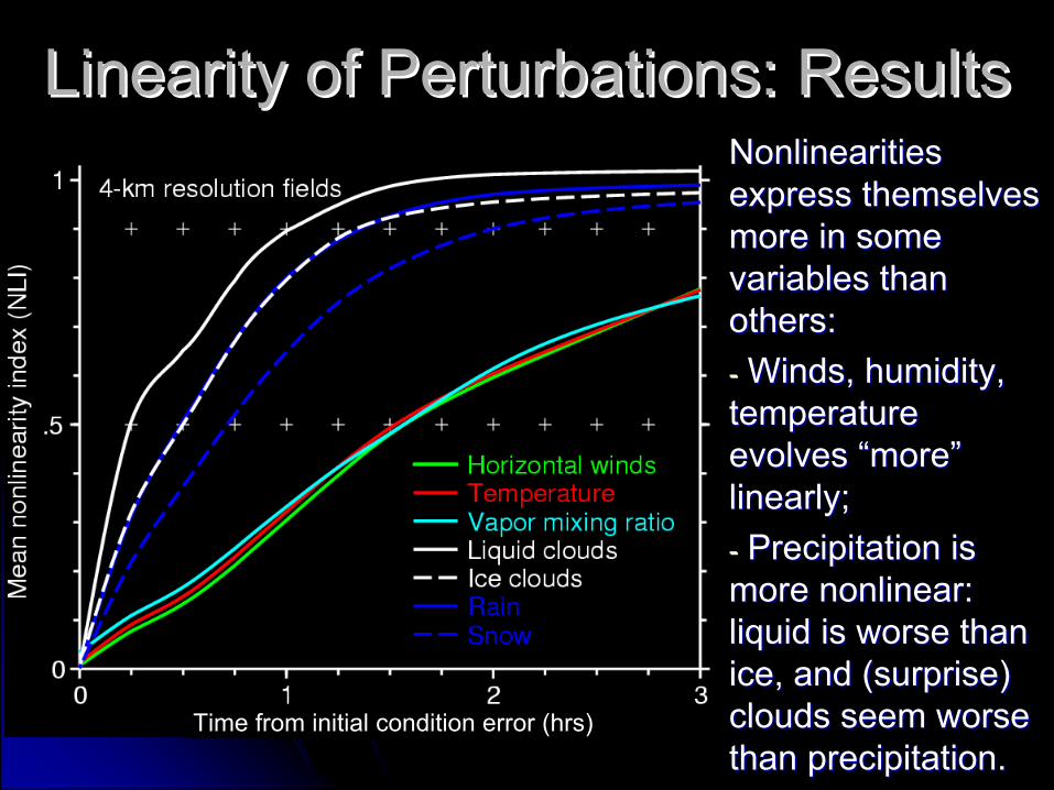
Linearity of Perturbations: ResultsLinearity of Perturbations: ResultsNonlinearities Nonlinearities express themselves express themselves more in some more in some variables than variables than others:others:--

Winds, humidity, Winds, humidity, temperature temperature evolves evolves ““moremore””

linearly;linearly;--

Precipitation is Precipitation is more nonlinear: more nonlinear: liquid is worse than liquid is worse than ice, and (surprise) ice, and (surprise) clouds seem worse clouds seem worse than precipitation.than precipitation.

Time from initial condition error (hrs)

Contradictory Information: ResultsContradictory Information: ResultsCII: Contradictory CII: Contradictory information indexinformation index

Results are similar Results are similar to nonlinear index; to nonlinear index; (but here rain is (but here rain is worse than clouds)worse than clouds)

Note: At CII = .11, Note: At CII = .11, oone (perfect) data ne (perfect) data point in ten is point in ten is worsening the initial worsening the initial state of the model.state of the model.

ingcontradict-non #pts ingcontradict #

=

Linearity of Perturbations: ResultsLinearity of Perturbations: ResultsIf assimilation is If assimilation is possible only when possible only when NLI<0.5 (threshold NLI<0.5 (threshold to be determined), to be determined), one can assimilate one can assimilate at 4at 4--km resolution:km resolution:

90 minutes of 90 minutes of winds, temperature winds, temperature and humidity data;and humidity data;

3030--45 minutes of 45 minutes of precipitation data;precipitation data;

1515--30 minutes of 30 minutes of cloud data.cloud data.

Note on nonlinearities and assimilation: both an assimilation and a modeling challenge

Time from initial condition error (hrs)

Linearity of Perturbations: ResultsLinearity of Perturbations: ResultsNonlinearities are a Nonlinearities are a function of scale function of scale

Smoothed fields Smoothed fields should be more should be more linear than higher linear than higher resolution fields.resolution fields.

Effect of smoothing:Effect of smoothing:--

Significant Significant (+100%)(+100%) predictability gains predictability gains

for winds, humidity, for winds, humidity, and temperature;and temperature;--

Some gains for Some gains for precipitation; limited precipitation; limited gains for cloudsgains for clouds

Time from initial condition error (hrs)

Assimilation and Predictability: Assimilation and Predictability: Partial ConclusionsPartial Conclusions

••

Clouds and precipitation patterns evolve highly Clouds and precipitation patterns evolve highly nonlinearly. nonlinearly. Using them to retrieve largerUsing them to retrieve larger--scale scale patterns of other variables will be challenging; sadly, patterns of other variables will be challenging; sadly, our best mesoscale sensors target these variables!our best mesoscale sensors target these variables!

••

Ideal assimilation strategy at the Ideal assimilation strategy at the mesoscalemesoscale

given given perfect measurements of model parameters:perfect measurements of model parameters:

1) smoothed 1) smoothed uu, , TT, , ee

for a few hours; 2) higherfor a few hours; 2) higher-- resolution resolution uu, , TT, , ee

for an hour; 3) for an hour; 3) RR

for 30 min; for 30 min; LWCLWC

for 15 min. Smoothed (for 15 min. Smoothed (uu

or or TT) and ) and ee

may be just may be just sufficient to constrain the largest subsufficient to constrain the largest sub--synoptic synoptic patterns; patterns; [Instrument[Instrument--related issues still have to be considered]related issues still have to be considered]

Assimilation and Predictability: Assimilation and Predictability: Partial ConclusionsPartial Conclusions

••

Assimilating variables with different predictability over Assimilating variables with different predictability over different periods may require more than plain 4Ddifferent periods may require more than plain 4D--Var.Var.

Scenario 1: Case reanalysisNo problems here.

3 hrs of smoothed u, T, e

1 hr of raw u, T, e

30 min of rain

15 min of clouds

Time of interest 3 hrs later

Assimilation and Predictability: Assimilation and Predictability: Partial ConclusionsPartial Conclusions

••

Assimilating variables with different predictability over Assimilating variables with different predictability over different periods may require more than plain 4Ddifferent periods may require more than plain 4D--Var.Var.

Scenario 2a: Real-time processingAssimilation does not take advantage

of the latest data available.Far from ideal

And assimilating 3 hrs of everything adds unusable non-linear “noise”

to usable “linear”

data and hurts more than helps.

3 hrs of smoothed u, T, e

1 hr of raw u, T, e

30 min of rain

15 min of clouds

Model time that 4D-var constrainswith assimilation

(3 hours ago) Present time

Assimilation and Predictability: Assimilation and Predictability: Partial ConclusionsPartial Conclusions

••

Assimilating variables with different predictability over Assimilating variables with different predictability over different periods may require more than plain 4Ddifferent periods may require more than plain 4D--Var.Var.

Scenario 2b: Real-time processingAssimilation of most fields will fail

because the data is several “predictability times”

away from the time for which the assimilation system is trying to adjust the initial

conditions of.

3 hrs of smoothed u, T, e

1 hr of raw u, T, e

30 min of rain

15 min of clouds

Model time that 4D-var constrainswith assimilation

(3 hours ago) Present time

Assimilation and Predictability: Assimilation and Predictability: Partial ConclusionsPartial Conclusions

••

Assimilating variables with different predictability over Assimilating variables with different predictability over different periods may require more than plain 4Ddifferent periods may require more than plain 4D--Var.Var.

Scenario 2c: Real-time processingIdeal solution, but it requires

deriving an approach that constrains the end time

of the assimilation window, not the beginning time as

traditional 4D-var does.

Possible? Or should multiple sliding assimilation windows be used?

3 hrs of smoothed u, T, e

1 hr of raw u, T, e

30 min of rain

15 min of clouds

Model time constrainedwith a to-be-determined

assimilation process

Present time +

Evaluating ObservationsEvaluating ObservationsQ: How much signal of the initial perturbation is Q: How much signal of the initial perturbation is

there in observations?there in observations?

It depends on how much an observation It depends on how much an observation yy

changes changes compared with the uncertainty compared with the uncertainty σσ((yy) ) in that in that observation and on the number of observations observation and on the number of observations made per unit time per instrument.made per unit time per instrument.

Signal strength: Signal strength:

( ) ( ) ( )[ ]( )∑ −+

=i i

iidataset y

TyTyTS 2

2,,,σ

xΔxxΔx

Evaluating ObservationsEvaluating ObservationsMany measurements were simulated: surface stations, Many measurements were simulated: surface stations,

raingaugesraingauges, , radiosondesradiosondes, microwave radiometers, , microwave radiometers, groundground--based GPS receivers, radars, and satellitebased GPS receivers, radars, and satellite--

borne IR images.borne IR images.

Signal strength per instrument per hour of data was Signal strength per instrument per hour of data was computed. Note that:computed. Note that:

•• Signal strength Signal strength ≠≠

UsefulnessUsefulness

•• Some quantities are harder to assimilate than Some quantities are harder to assimilate than others: complex link between measurement and others: complex link between measurement and atmospheric parameter (e.g., Z atmospheric parameter (e.g., Z LWC)LWC), data , data difficult to simulate (e.g., surface measurements)difficult to simulate (e.g., surface measurements)……

Signal Strength ResultsSignal Strength Results

Dashed: NLI > .5Dotted: NLI > .9

Tentative RecommendationsTentative RecommendationsFor instrument developers:For instrument developers:

••

Aim at midlevel moisture; then low and midlevel temperature.Aim at midlevel moisture; then low and midlevel temperature.

For data assimilation researchers:For data assimilation researchers:

••

Ideal assimilation strategy at the mesoscale: 1) smoothed Ideal assimilation strategy at the mesoscale: 1) smoothed winds, temperature, moisture for a few hours; 2) higherwinds, temperature, moisture for a few hours; 2) higher--

resolution winds, temperature, moisture for one hour; 3) radar resolution winds, temperature, moisture for one hour; 3) radar reflectivity for 10 min; 4) one thermalreflectivity for 10 min; 4) one thermal--IR satellite image;IR satellite image;

••

Different initial condition variables should be constrained withDifferent initial condition variables should be constrained with different assimilation windows. New 4Ddifferent assimilation windows. New 4D--Var formalism needed?Var formalism needed?

To be explored (not by me!):To be explored (not by me!):

••

How tolerant are different assimilation approaches to variables How tolerant are different assimilation approaches to variables that evolve nonlinearly?that evolve nonlinearly?

Questions Unanswered in this WorkQuestions Unanswered in this Work

••

How many perturbations of initial conditions How many perturbations of initial conditions result in similar signals on observations? result in similar signals on observations? (beyond the scope of this study)(beyond the scope of this study)

••

How to use and not misuse the results How to use and not misuse the results presented here (I still need to think about this)presented here (I still need to think about this)

THE END (?)