Embed Size (px)
Citation preview

Prolog Programming
A First Course
Paul Brna
March 5, 2001

Abstract
The course for which these notes are designed is intended for undergraduatestudents who have some programming experience and may even have writtena few programs in Prolog. They are not assumed to have had any formalcourse in either propositional or predicate logic.
At the end of the course, the students should have enough familiarity withProlog to be able to pursue any undergraduate course which makes use ofProlog.
This is a rather ambitious undertaking for a course of only twelve lecturesso the lectures are supplemented with exercises and small practical projectswherever possible.
The Prolog implementation used is SICStus Prolog which is closely mod-elled on Quintus Prolog (SICS is the Swedish Institute of Computer Science).The reference manual should also be available for consultation [SICStus, 1988].
c©Paul Brna 1988

Contents
1 Introduction 1
1.1 Declarative vs Procedural Programming . . . . . . . . . . . . 1
1.2 What Kind of Logic? . . . . . . . . . . . . . . . . . . . . . . . 1
1.3 A Warning . . . . . . . . . . . . . . . . . . . . . . . . . . . . 2
1.4 A Request . . . . . . . . . . . . . . . . . . . . . . . . . . . . . 2
2 Knowledge Representation 3
2.1 Propositional Calculus . . . . . . . . . . . . . . . . . . . . . . 3
2.2 First Order Predicate Calculus . . . . . . . . . . . . . . . . . 4
2.3 We Turn to Prolog . . . . . . . . . . . . . . . . . . . . . . . 5
2.4 Prolog Constants . . . . . . . . . . . . . . . . . . . . . . . . 7
2.5 Goals and Clauses . . . . . . . . . . . . . . . . . . . . . . . . 8
2.6 Multiple Clauses . . . . . . . . . . . . . . . . . . . . . . . . . 8
2.7 Rules . . . . . . . . . . . . . . . . . . . . . . . . . . . . . . . . 9
2.8 Semantics . . . . . . . . . . . . . . . . . . . . . . . . . . . . . 10
2.9 The Logical Variable . . . . . . . . . . . . . . . . . . . . . . . 11
2.10 Rules and Conjunctions . . . . . . . . . . . . . . . . . . . . . 12
2.11 Rules and Disjunctions . . . . . . . . . . . . . . . . . . . . . . 13
2.12 Both Disjunctions and Conjunctions . . . . . . . . . . . . . . 14
2.13 What You Should Be Able To Do . . . . . . . . . . . . . . . . 15
3 Prolog’s Search Strategy 16
3.1 Queries and Disjunctions . . . . . . . . . . . . . . . . . . . . 16
3.2 A Simple Conjunction . . . . . . . . . . . . . . . . . . . . . . 19
3.3 Conjunctions and Disjunctions . . . . . . . . . . . . . . . . . 21
3.4 What You Should Be Able To Do . . . . . . . . . . . . . . . . 23
4 Unification, Recursion and Lists 26
4.1 Unification . . . . . . . . . . . . . . . . . . . . . . . . . . . . 26
4.2 Recursion . . . . . . . . . . . . . . . . . . . . . . . . . . . . . 27
4.3 Lists . . . . . . . . . . . . . . . . . . . . . . . . . . . . . . . . 29
4.4 What You Should Be Able To Do . . . . . . . . . . . . . . . . 32
i

ii
5 The Box Model of Execution 34
5.1 The Box Model . . . . . . . . . . . . . . . . . . . . . . . . . . 34
5.2 The Flow of Control . . . . . . . . . . . . . . . . . . . . . . . 35
5.3 An Example using the Byrd Box Model . . . . . . . . . . . . 36
5.4 An Example using an AND/OR Proof Tree . . . . . . . . . . 38
5.5 What You Should Be Able To Do . . . . . . . . . . . . . . . . 38
6 Programming Techniques and List Processing 53
6.1 The ‘Reversibility’ of Prolog Programs . . . . . . . . . . . . 53
6.1.1 Evaluation in Prolog . . . . . . . . . . . . . . . . . . 54
6.2 Calling Patterns . . . . . . . . . . . . . . . . . . . . . . . . . 55
6.3 List Processing . . . . . . . . . . . . . . . . . . . . . . . . . . 56
6.3.1 Program Patterns . . . . . . . . . . . . . . . . . . . . 56
6.3.2 Reconstructing Lists . . . . . . . . . . . . . . . . . . . 60
6.4 Proof Trees . . . . . . . . . . . . . . . . . . . . . . . . . . . . 62
6.5 What You Should Be Able To Do . . . . . . . . . . . . . . . . 63
7 Control and Negation 66
7.1 Some Useful Predicates for Control . . . . . . . . . . . . . . . 66
7.2 The Problem of Negation . . . . . . . . . . . . . . . . . . . . 67
7.2.1 Negation as Failure . . . . . . . . . . . . . . . . . . . . 68
7.2.2 Using Negation in Case Selection . . . . . . . . . . . . 69
7.3 Some General Program Schemata . . . . . . . . . . . . . . . . 70
7.4 What You Should Be Able To Do . . . . . . . . . . . . . . . . 77
8 Parsing in Prolog 78
8.1 Simple English Syntax . . . . . . . . . . . . . . . . . . . . . . 78
8.2 The Parse Tree . . . . . . . . . . . . . . . . . . . . . . . . . . 79
8.3 First Attempt at Parsing . . . . . . . . . . . . . . . . . . . . 80
8.4 A Second Approach . . . . . . . . . . . . . . . . . . . . . . . 81
8.5 Prolog Grammar Rules . . . . . . . . . . . . . . . . . . . . . 82
8.6 To Use the Grammar Rules . . . . . . . . . . . . . . . . . . . 83
8.7 How to Extract a Parse Tree . . . . . . . . . . . . . . . . . . 83
8.8 Adding Arbitrary Prolog Goals . . . . . . . . . . . . . . . . 84
8.9 What You Should Be Able To Do . . . . . . . . . . . . . . . . 84
9 Modifying the Search Space 86
9.1 A Special Control Predicate . . . . . . . . . . . . . . . . . . . 86
9.1.1 Commit . . . . . . . . . . . . . . . . . . . . . . . . . . 86
9.1.2 Make Determinate . . . . . . . . . . . . . . . . . . . . 89
9.1.3 Fail Goal Now . . . . . . . . . . . . . . . . . . . . . . 90

iii
9.2 Changing the Program . . . . . . . . . . . . . . . . . . . . . . 91
9.2.1 Do Not Do It! . . . . . . . . . . . . . . . . . . . . . . . 92
9.2.2 Sometimes You have To! . . . . . . . . . . . . . . . . . 93
9.3 What You Should Be Able To Do . . . . . . . . . . . . . . . . 94
10 Prolog Syntax 97
10.1 Constants . . . . . . . . . . . . . . . . . . . . . . . . . . . . . 97
10.2 Variables . . . . . . . . . . . . . . . . . . . . . . . . . . . . . 98
10.3 Compound Terms . . . . . . . . . . . . . . . . . . . . . . . . . 98
10.4 (Compound) Terms as Trees . . . . . . . . . . . . . . . . . . . 99
10.5 Compound Terms and Unification . . . . . . . . . . . . . . . 99
10.6 The Occurs Check . . . . . . . . . . . . . . . . . . . . . . . . 100
10.7 Lists Are Terms Too . . . . . . . . . . . . . . . . . . . . . . . 101
10.8 How To Glue Two Lists Together . . . . . . . . . . . . . . . . 102
10.9 Rules as Terms . . . . . . . . . . . . . . . . . . . . . . . . . . 104
10.10What You Should Be Able To Do . . . . . . . . . . . . . . . . 105
11 Operators 112
11.1 The Three Forms . . . . . . . . . . . . . . . . . . . . . . . . . 112
11.1.1 Infix . . . . . . . . . . . . . . . . . . . . . . . . . . . . 112
11.1.2 Prefix . . . . . . . . . . . . . . . . . . . . . . . . . . . 113
11.1.3 Postfix . . . . . . . . . . . . . . . . . . . . . . . . . . . 113
11.2 Precedence . . . . . . . . . . . . . . . . . . . . . . . . . . . . 113
11.3 Associativity Notation . . . . . . . . . . . . . . . . . . . . . . 116
11.3.1 Infix Operators . . . . . . . . . . . . . . . . . . . . . . 116
11.3.2 The Prefix Case . . . . . . . . . . . . . . . . . . . . . 117
11.3.3 Prefix Operators . . . . . . . . . . . . . . . . . . . . . 117
11.3.4 Postfix Operators . . . . . . . . . . . . . . . . . . . . . 117
11.4 How to Find Operator Definitions . . . . . . . . . . . . . . . 117
11.5 How to Change Operator Definitions . . . . . . . . . . . . . . 118
11.6 A More Complex Example . . . . . . . . . . . . . . . . . . . . 119
11.7 What You Should Be Able To Do . . . . . . . . . . . . . . . . 120
12 Advanced Features 122
12.1 Powerful Features . . . . . . . . . . . . . . . . . . . . . . . . . 122
12.1.1 Powerful Features —Typing . . . . . . . . . . . . . . . 122
12.1.2 Powerful Features —Splitting Up Clauses . . . . . . . 123
12.1.3 Powerful Features —Comparisons of Terms . . . . . . 128
12.1.4 Powerful Features —Finding All Solutions . . . . . . . 128
12.1.5 Powerful Features —Find Out about Known Terms . 130

iv
12.2 Open Lists and Difference Lists . . . . . . . . . . . . . . . . . 131
12.3 Prolog Layout . . . . . . . . . . . . . . . . . . . . . . . . . . 136
12.3.1 Comments . . . . . . . . . . . . . . . . . . . . . . . . . 136
12.4 Prolog Style . . . . . . . . . . . . . . . . . . . . . . . . . . . 138
12.4.1 Side Effect Programming . . . . . . . . . . . . . . . . 138
12.5 Prolog and Logic Programming . . . . . . . . . . . . . . . . 140
12.5.1 Prolog and Resolution . . . . . . . . . . . . . . . . . 140
12.5.2 Prolog and Parallelism . . . . . . . . . . . . . . . . . 140
12.5.3 Prolog and Execution Strategies . . . . . . . . . . . . 141
12.5.4 Prolog and Functional Programming . . . . . . . . . 141
12.5.5 Other Logic Programming Languages . . . . . . . . . 141
12.6 What You Should Be Able To Do . . . . . . . . . . . . . . . . 141
A A Short Prolog Bibliography 142
B Details of the SICStus Prolog Tracer 145
C Solutions and Comments on Exercises for Chapter ?? 148
C.1 Exercise 2.1 . . . . . . . . . . . . . . . . . . . . . . . . . . . . 148
C.2 Execise 2.2 . . . . . . . . . . . . . . . . . . . . . . . . . . . . 149
C.3 Exercise 2.3 . . . . . . . . . . . . . . . . . . . . . . . . . . . . 150
C.4 Exercise 2.4 . . . . . . . . . . . . . . . . . . . . . . . . . . . . 150
C.5 Exercise 2.5 . . . . . . . . . . . . . . . . . . . . . . . . . . . . 151
C.6 Exercise 2.6 . . . . . . . . . . . . . . . . . . . . . . . . . . . . 152
C.7 Exercise 2.7 . . . . . . . . . . . . . . . . . . . . . . . . . . . . 152
D Solutions and Comments on Exercises for Chapter ?? 155
D.1 Exercise 3.1 . . . . . . . . . . . . . . . . . . . . . . . . . . . . 155
D.2 Exercise 3.2 . . . . . . . . . . . . . . . . . . . . . . . . . . . . 156
E Solutions and Comments on Exercises for Chapter ?? 160
E.1 Exercise 4.1 . . . . . . . . . . . . . . . . . . . . . . . . . . . . 160
E.2 Exercise 4.2 . . . . . . . . . . . . . . . . . . . . . . . . . . . . 160
E.3 Exercise 4.3 . . . . . . . . . . . . . . . . . . . . . . . . . . . . 162
F Solutions and Comments on Exercises for Chapter ?? 165
F.1 Exercise 6.1 . . . . . . . . . . . . . . . . . . . . . . . . . . . . 165
G Solutions and Comments on Exercises for Chapter ?? 175
G.1 Exercise 8.1 . . . . . . . . . . . . . . . . . . . . . . . . . . . . 175
H Solutions and Comments on Exercises for Chapter ?? 178
H.1 Exercise 9.1 . . . . . . . . . . . . . . . . . . . . . . . . . . . . 178

I Solutions and Comments on Exercises for Chapter ?? 183
I.1 Exercise 11.1 . . . . . . . . . . . . . . . . . . . . . . . . . . . 183
J Solutions and Comments on Exercises for Chapter ?? 184
J.1 Exercise 12.1 . . . . . . . . . . . . . . . . . . . . . . . . . . . 184

List of Figures
3.1 A Failed Match . . . . . . . . . . . . . . . . . . . . . . . . . . 18
3.2 A Successful Match . . . . . . . . . . . . . . . . . . . . . . . . 20
5.1 The Byrd Box Model Illustrated . . . . . . . . . . . . . . . . 34
5.2 Illustrating Simple Flow of Control . . . . . . . . . . . . . . . 36
5.3 Program Example with Byrd Box Representation . . . . . . . 37
5.4 The AND/OR Tree for the Goal a(X,Y) . . . . . . . . . . . 38
5.5 The Development of the AND/OR Proof Tree . . . . . . . . . 39
5.6 Yuppies on the Move . . . . . . . . . . . . . . . . . . . . . . . 52
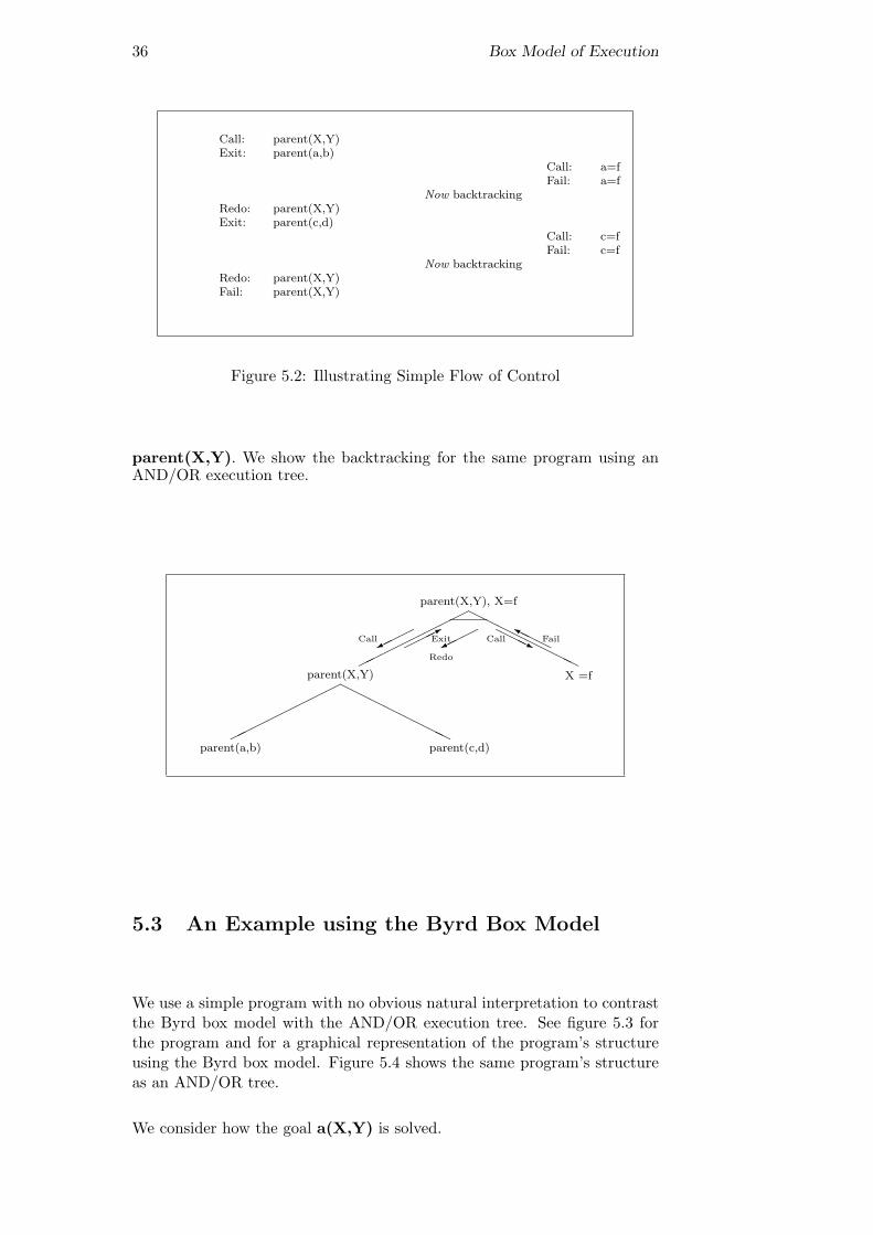
6.1 The Proof Tree for triple([1,2],Y) . . . . . . . . . . . . . . . 62
6.2 The Proof Tree for triple([1,2],[],Y) . . . . . . . . . . . . . 63
8.1 A Parse Tree . . . . . . . . . . . . . . . . . . . . . . . . . . . 79
9.1 The Effect of cut on the AND/OR Tree . . . . . . . . . . . . 88
9.2 The First Solution to the Goal sum(2,Ans) . . . . . . . . . 90
9.3 Resatisfying the Goal sum(2,Ans) . . . . . . . . . . . . . . . 91
9.4 The Effect of the cut on the Goal sum(2,Ans) . . . . . . . . 92

Preface
A Warning
These notes are under development. Much will eventually change. Pleasehelp to make these notes more useful by letting the author know of anyerrors or missing information. Help future generations of AI2 students!
The Intended Audience
The course for which these notes are designed is intended for undergraduatestudents who have some programming experience and may even have writtena few programs in Prolog. They are not assumed to have had any formalcourse in either propositional or predicate logic.
The Objective
At the end of the course, the students should have enough familiarity withProlog to be able to pursue any undergraduate course which makes use ofProlog.
The original function was to provide students studying Artificial Intelligence(AI) with an intensive introduction to Prolog so, inevitably, there is a slightbias towards AI.
The Aims
At the end of the course the students should be:
• familiar with the basic syntax of the language
• able to give a declarative reading for many Prolog programs
• able to give a corresponding procedural reading
• able to apply the fundamental programming techniques
• familiar with the idea of program as data
• able to use the facilities provided by a standard trace package to debugprograms
• familiar with the fundamental ideas of the predicate calculus
• familiar with the fundamental ideas specific to how Prolog works
vii

viii
Course Structure
This is a rather ambitious undertaking for a course of only twelve lecturesso the lectures are supplemented with exercises and small practical projectswherever possible.
Acknowledgements
These notes are based on a previous version used with the students of the AI2course in Prolog during the session 1985–87 and 1988–89 at the Departmentof Artificial Intelligence, Edinburgh University. My thanks for the feedbackthat they supplied.

Chapter 1
Introduction
intro-chap
Prolog is PROgramming in LOGic
A few points must be cleared up before we begin to explore the main aspectsof Prolog.
These notes are supplemented with exercises and suggestions for simple prac-ticals. It is assumed that you will do most of this supplementary work eitherin your own time, for tutorials or during practical sessions.
Each chapter will start with a simple outline of its content and finish witha brief description of what you should know upon completion of the chapterand its exercises.
Important points will be boxed and some technical and practical detailswhich are not immediately essential to the exposition will be
written in a smaller font.
1.1 Declarative vs Procedural Programming
Procedural programming requires that the programmer tell the computerwhat to do. That is, how to get the output for the range of required inputs.The programmer must know an appropriate algorithm.
Declarative programming requires a more descriptive style. The programmermust know what relationships hold between various entities.
Pure1 Prolog allows a program to be read either declaratively or procedu-rally. This dual semantics is attractive.
1.2 What Kind of Logic?
Prolog is based on First Order Predicate Logic —sometimes abbreviatedto FOPL.
1Prolog, like LISP, has a pure subset of features. The implication is that some featuresof both languages are regarded as impure —these are often provided for efficiency or foruseful, but strictly unnecessary features. The impure features of Prolog damage thepleasing equality between the declarative and procedural readings of Prolog programs.
1

2 Introduction to Prolog
First order predicate logic implies the existence of a set of predicate symbolsalong with a set of connectives.
First order predicate logic implies that there is no means provided for “talk-ing about” the predicates themselves.
Prolog is based on FOPL but uses a restricted version of the clausal form.Clausal form is a particular way of writing the propositions of FOPL. Therestriction is known as Horn clause form.
Prolog is a so-called logic programming language. Strictly, it is not the onlyone but most such languages are its descendents.
We will spend a little time outlining the basic ideas underlying both proposi-tional and predicate logic. It is not the intention to use Prolog as a vehicleto teach logic but some appreciation of the issues is invaluable.
1.3 A Warning
Prolog is known to be a difficult language to master. It does not have thefamiliar control primitives used by languages like RATFOR, ALGOL andPASCAL so the system does not give too much help to the programmer toemploy structured programming concepts.
Also, many programmers have become used to strongly typed languages.Prolog is very weakly typed indeed. This gives the programmer great powerto experiment but carries the obvious responsibility to be careful.
Another major difference is the treatment of variables —special attentionshould be given to understanding variables in Prolog.
Prolog provides a search strategy for free —there is a cost. The program-mer has to develop a methodology to handle the unexpected consequencesof a faulty program. In particular, pay careful attention to the issue ofbacktracking.
It is usual to assume that telling people how they can go wrong is an en-couragement to do exactly that —go wrong. The approach taken here is tomake the known difficulties explicit.
1.4 A Request
These notes are slowly being improved. Many further exercises need to beadded along with more example programs and improvements to the text.
If you have any comments that will help in the development of these notesthen please send your comments to:
Paul BrnaDepartment of Artificial IntelligenceUniversity of Edinburgh80 South BridgeEdinburgh EH1 1HN

Chapter 2
Knowledge Representation
KRchapter
We take a very brief and informal look at both the propositionalcalculus and first order predicate logic.We then restrict our attention to a form of predicate logic whichtranslates directly into Prolog.This requires that we introduce a simple vocabulary that de-scribes the syntax of Prolog.Here, we concentrate on an informal description of the funda-mental units which are:
clause, rule, fact,goal, subgoal,logical variable, constant, atom,functor, argument, arity.
An explanation as to how statements can be represented inProlog form is given.
How do we represent what we know? The simplest analysis requires that wedistinguish between knowledge how –procedural knowledge such as how todrive a car— and knowledge that —declarative knowledge such as knowingthe speed limit for a car on a motorway.
Many schemes for representing knowledge have been advanced —includingfull first order predicate logic. The strong argument for classical (first orderpredicate) logic is that it has a well understood theoretical foundation.
2.1 Propositional Calculus
The propositional calculus is based on statements which have truth values(true or false).
The calculus provides a means of determining the truth values associatedwith statements formed from “atomic” statements. An example:
If p stands for “fred is rich” and q for “fred is tall” then we may form state-ments such as:
3

4 Knowledge Representation
Symbolic Statement Translationp ∨ q p or qp ∧ q p and qp ⇒ q p logically implies qp ⇔ q p is logically equivalent to q¬p not p
Note that ∨, ∧, ⇒ and ⇔ are all binary connectives. They are sometimesreferred to, respectively, as the symbols for disjunction, conjunction, impli-cation and equivalence. Also, ¬ is unary and is the symbol for negation.
If propositional logic is to provide us with the means to assess the truthvalue of compound statements from the truth values of the ‘building blocks’then we need some rules for how to do this.
For example, the calculus states that p∨q is true if either p is true or q istrue (or both are true). Similar rules apply for all the ways in which thebuilding blocks can be combined.
A Problem
If p stands for “all dogs are smelly” and p is true then we would like to beable to prove that “my dog fido is smelly”.
We need to be able to get at the structure and meaning of statements. Thisis where (first order1) predicate logic is useful.
2.2 First Order Predicate Calculus
The predicate calculus includes a wider range of entities. It permits thedescription of relations and the use of variables. It also requires an under-standing of quantification.
The language of predicate calculus requires:
Variables
Constants —these include the logical constants
Symbol Meaning∨ or∧ and¬ not⇒ logically implies⇔ logically equivalent∀ for all∃ there exists
The last two logical constants are additions to the logical connectivesof propositional calculus —they are known as quantifiers. The non-logical constants include both the ‘names’ of entities that are relatedand the ‘names’ of the relations. For example, the constant dog mightbe a relation and the constant fido an entity.
1Do not worry about the term first order for now. Much later on, it will becomerelevant.

5
Predicate —these relate a number of entities. This number is usuallygreater than one. A predicate with one argument is often used toexpress a property e.g. sun(hot) may represent the statement that“the sun has the property of being hot”.
If there are no arguments then we can regard the ‘predicate’ as stand-ing for a statement a la the propositional calculus.
Formulæ —these are constructed from predicates and formulæ2. The log-ical constants are used to create new formulæ/ from old ones. Hereare some examples:
Formula(e) New Formuladog(fido) ¬ dog(fido)dog(fido) and old(fido) dog(fido)∨ old(fido)dog(fido) and old(fido) dog(fido)∧ old(fido)dog(fido) and old(fido) dog(fido)⇒ old(fido)dog(fido) and old(fido) dog(fido)⇔ old(fido)dog(X) ∀X.dog(X)dog(X) ∃X.dog(X)
Note that the word “and” used in the left hand column is used tosuggest that we have more than one formula for combination —andnot necessarily a conjunction.
In the last two examples, “dog(X)” contains a variable which is saidto be free while the “X” in “∀X.dog(X)” is bound.
Sentence —a formula with no free variables is a sentence.
Two informal examples to illustrate quantification follow:
∀X.(man(X)⇒mortal(X)) All men are mortal∃X.elephant(X) There is at least one elephant
The former is an example of universal quantification and the latter of exis-tential quantification.
We can now represent the problem we initially raised:
∀X.(dog(X)⇒smelly(X))∧dog(fido)⇒smelly(fido)
To verify that this is correct requires that we have some additional machinerywhich we will not discuss here.
2.3 We Turn to Prolog
Prolog provides for the representation of a subset of first order predicatecalculus. The restrictions on what can be done will become clearer later.We will now explain how we can write logical statements in Prolog.
2Note that this is a recursive definition.

6 Knowledge Representation
If “the capital of france is paris” then we can represent this in predicatecalculus form as3:
france has capital paris
We have a binary relationship (two things are related) written in infix form.That is, the relationship is written between the two things related.
The relationship (or predicate) has been given the name “has capital” —hence we say that the predicate name is “has capital”.
And in Prolog form by such as:
has capital(france,paris).
where we write a prefix form and say that the relationship takes two argu-ments. Prefix because the relationship is indicated before the two relatedthings.
Note that, in Prolog, if the name of an object starts with a lower case letterthen we refer to a specific object. Also, there must be no space between thepredicate name and the left bracket “(”. The whole thing also ends in a “.”as the last character on the line.
The exact rule for the termination of a clause is that a clause must endwith a “.” followed by white space where white space can be any of{space,tab,newline,end of file}. It is safest to simply put “.” followedby newline.
Also note that relations do not need to hold between exactly two objects.For example,
meets(fred,jim,bridge)
might be read as
fred meets jim by the bridge
Here, three objects are related so it makes little sense to think of the relationmeets as binary —it is ternary.
If we can relate two objects or three then it is reasonable to relate n wheren ≥ 2. Is there any significance to a relationship that relates one or evenzero objects? A statement like
jim is tall
might be represented either as3The failure to capitalise “france” and “paris” is quite deliberate. In Prolog, named,
specific objects (i.e. the atoms) usually start with a lower case letter.

7
tall(jim)
or
jim(tall)
It is, perhaps, preferable to see tallness as being a property which is pos-sessed by jim.
A ‘relation’ that has no arguments can be seen as a single proposition. Thusthe binary relation “france has capital paris” above might be rewritten asthe statement “france has capital paris” —a relation with no arguments.
2.4 Prolog Constants
If we have
loves(jane,jim).
then jane and jim refer to specific objects. Both jane and jim are con-stants. In particular, in DEC-10 Prolog terminology, both are atoms. Also,“loves” happens to be an atom too because it refers to a specific relationship.Generally speaking, if a string of characters starts with a lower case letter,the DEC-10 family of Prologs assume that the entity is an atom.
There are constants other than atoms —including integers and real numbers.
A constant is an atom or a number. A number is an integer or a realnumber4. The rules for an atom are quite complicated:
quoted item ’anything but the single quote character’word lower case letter followed by any letter, digit or (underscore)symbol any number of {+, -, *, /, \, ^, <, >, =, ’, ~, :, ., ?, @, #, $, &}special item any of { [], {}, ;, !, %}
So the following are all atoms:
likes chocolate, fooX23, ++*++, ::=, ’What Ho!’
By the way, you can include a single quote within a quoted atom —justduplicate the single quote. This gives the quoted atom with a singlequote as:
’’’’
A practical warning: remember to pair off your (single) quote signswhen inputing a quoted atom or Prolog may keep on swallowing yourinput looking for that elusive single quote character. This is one of themost common syntactic errors for beginners.While we are on the subject, another common error is to assume thata double quote (") behaves like a single quote —i.e. that the term"Hello" is an atom just like ’Hello’. This is not so. When you dofind out what sensible things can be done with the double quote thenremember to pair them off.
4Referred to as a float in the SICStus Prolog manual [SICStus, 1988].

8 Knowledge Representation
Because Prolog is modelled on a subset of first order predicate logic, allpredicate names must be constants —but not numbers. In particular,
No predicate may be a variable
That is, we cannot have X(jane,jim) as representing the fact that janeand jim are related in some unknown way.
2.5 Goals and Clauses
We distinguish between a Prolog goal and Prolog clause. A clause is thesyntactic entity expressing a relationship as required by Prolog —note thatwe will regard the ‘.’ as terminating a clause (this is not strictly correct).
loves(jane,jim) is a goalloves(jane,jim). is a unit clause
The adjectives unit and non-unit distinguish two kinds of clause —intuitively,facts and rules respectively.
Exercise 2.1 Here is the first opportunity to practice the representation ofsome statement in Prolog form.
1. bill likes ice-cream
2. bill is tall
3. jane hits jimmy with the cricket bat
4. john travels to london by train
5. bill takes jane some edam cheese
6. freddy lives at 16 throgmorton street in london
The failure to capitalise “freddy”, “london” etc. is a reminder that the ver-sion of Prolog that we are using requires that constants should not startwith an upper case letter.
Note that there may be several ways of representing each of these statements.
2.6 Multiple Clauses
A predicate may be defined by a set of clauses with the same predicate nameand the same number of arguments.
We will therefore informally describe the way in which this is handledthrough an example. The logical statement (in first order form)
squared(1,1)∧squared(2,4)∧squared(3,9)
is to be represented as three distinct Prolog clauses.

9
squared(1,1).squared(2,4).squared(3,9).
Note that this way of turning a conjunctive statement into Prolog is oneof the fundamental restrictions previously mentioned. There are more tofollow.
All the above clauses are unit clauses —this is not a necessary requirement.See section 2.12 for an example with both unit and non-unit clauses.
We now introduce a graphical representation which will be used in a numberof different ways. The idea we use here is to represent a program (in thiscase, consisting of a set of unit clauses) as a tree.
•
squared(1,1) squared(2,4) squared(3,9)
(((((((((((((
hhhhhhhhhhhhh
This tree is an example of an OR tree.
It might have been expected that we would call this an AND tree but, whenwe are trying to determine whether a statement such as squared(1,1) istrue then we might use either the first clause or the second or the third andso on.
Exercise 2.2 Represent each of these statements as a set of Prolog clauses.
1. bill only eats chocolate, bananas or cheese.
2. the square root of 16 is 4 or -4.
3. wales, ireland and scotland are all countries.
2.7 Rules
The format is:
divisible by two:-even.
This is a non-unit clause.
In general, a clause consists of two parts: the head and the body5.
The head is divisible by two and the body is even —even is sometimesreferred to as a subgoal.
5These two body parts are ‘joined’ by the neck. There is an analogous concept in theProlog literature.

10 Knowledge Representation
Note that the symbol “:-” is read as if. An informal reading of the clause is“divisible by two is true if even is true” which is equivalent to “even⇒ divisible by two”.
Any number of subgoals may be in the body of the rule.
No more than one goal is allowed in the head
This is another way in which Prolog is a restriction of full first order predi-cate calculus. For example, we cannot translate rich(fred)⇒ happy(fred)∧powerful(fred)directly into the Prolog version happy(fred),powerful(fred) :- rich(fred).
See section 2.10 for an example of a clause with more than one subgoal inthe body. A fact is effectively a rule with no subgoals.
You may have noticed that, even if it is held that “even” is a relation, itdoes not seem to relate anything to anything else.
The rule is not as much use as it might be because it does not reveal themore interesting relationship that
A number is divisible by two if it is even
We can express this with the help of the logical variable. Here is the im-proved rule:
divisible by two(X):-even(X).
This is also a non-unit clause. The named logical variable is X. This Prologclause is equivalent to the predicate calculus statement ∀ X. (even(X) ⇒divisible by two(X)).
2.8 Semantics
Here is an informal version of the procedural semantics for the exampleabove:
If we can find a value of X that satisfies the goal even(X)then we have also found a number that satisfies the goal di-visible by two(X).
The declarative semantics.
If we can prove that X is “even” then we have proved that X is“divisible by two”.
Note that there is an implicit universal quantification here. That is,for all objects those that are even are also divisible by two.
∀X.(even(X)⇒ divisible by two(X))
Also note that the head goal is found on the right of the standard logicalimplication symbol. It is a common error to reverse the implication.

11
Two final examples of a single rule. The first:
all scots people are british
can be turned into:
british(Person):-scottish(Person).
Note that Person is another logical variable. Now for the final example:
if you go from one country to another they you are a tourist
turns into:
tourist(P):-move(P,Country1,Country2).
where move(P,A,B) has the informal meaning that a person P has movedfrom country A to country B.
There is a problem here. We really need to specify that Country1 andCountry2 are legitimate and distinct countries6.
Exercise 2.3 Represent these statements as single non-unit clauses (rules):
1. all animals eat custard
2. everyone loves bergman’s films
3. jim likes fred’s possessions
4. if someone needs a bike then they may borrow jane’s
2.9 The Logical Variable
In the DEC-10 Prolog family, if an object is referred to by a name startingwith a capital letter then the object has the status of a logical variable. Inthe above rule there are two references to X. All this means is that the tworeferences are to the same object —whatever that object is.
The scope rule for Prolog is that two uses of an identical name for a logicalvariable only refer to the same object if the uses are within a single clause.Therefore in
6This could be enforced by the move/3 relation (predicate) but this would producean unnaturally specific version of moving. The real solution is to provide some predicatesuch as not same/2 which has the meaning that not same(P1,P2) precisely when P1is not the same as P2.

12 Knowledge Representation
happy(X):-healthy(X).
wise(X):-old(X).
the two references to X in the first clause do not refer to the same object asthe references to X in the second clause. By the way, this example is a sortthat is discussed in section 2.11.
Do not assume that the word logical is redundant. It is used to distinguishbetween the nature of the variable as used in predicate calculus and thevariable used in imperative languages like BASIC, FORTRAN, ALGOL andso on. In those languages, a variable name indicates a storage location whichmay ‘contain’ different values at different moments in the execution of theprogram.
The logical variable cannot be overwritten with a new value
Although this needs some further comments, it is probably better to startwith this statement and qualify it later.
For example, in Pascal:
X:= 1; X:= 2;
results in the assignment of 2 to X. In Prolog, once a logical variablehas a value, then it cannot be assigned a different one. The logicalstatement
X=1 ∧ X=2
cannot be true as X cannot be both ‘2’ and ‘1’ simultaneously. Anattempt to make a logical variable take a new value will fail.
2.10 Rules and Conjunctions
A man is happy if he is rich and famous
might translate to:
happy(Person):-man(Person),rich(Person),famous(Person).
The ‘,’ indicates the conjunction and is roughly equivalent to the ∧ of pred-icate calculus. Therefore, read ‘,’ as ‘and’7. The whole of the above is one(non-unit) single clause.
It has three subgoals in its body —these subgoals are ‘conjoined’.7It’s meaning is more accurately captured by the procedural ‘and then’.

13
In this single clause, the logical variable Person refers to the same objectthroughout.
By the way, we might have chosen any name for the logical variable otherthan Person. It is common practice to name a logical variable in some waythat reminds you of what kind of entity is being handled.
We now describe this clause graphically. In this case, we are going to repre-sent conjunctions using an AND tree. Here is an AND tree that representsthe above.
•
man(Person) rich(Person) famous(Person)
(((((((((((((
hhhhhhhhhhhhh
The way in which we discriminate between an OR tree and an AND tree isthe use of a horizontal bar to link the subgoals. We need this distinction be-cause we are going to represent the structure of a program using a combinedAND/OR tree.
Exercise 2.4 A few more exercises. Each of these statements should beturned into a rule (non-unit clause) with at least two subgoals —even thoughsome statements are not immediately recognisable as such:
1. you are liable to be fined if your car is untaxed
2. two people live in the same house if they have the same address
3. two people are siblings if they have the same parents
2.11 Rules and Disjunctions
Someone is happy if they are healthy, wealthy or wise.
translates to:
happy(Person):-healthy(Person).
happy(Person):-wealthy(Person).
happy(Person):-wise(Person).
Note how we have had to rewrite the original informal statement into some-thing like:
Someone is happy if they are healthy ORSomeone is happy if they are wealthy ORSomeone is happy if they are wise

14 Knowledge Representation
We have also assumed that each clause is (implicitly) universally quantified.i.e. the first one above represents ∀X.(healthy(X)⇒happy(X)).
The predicate name “happy’ is known as a functor.
The functor happy has one argument.
We describe a predicate with name “predname” with arity “n” as pred-name/n. It has one argument —we say its arity is 1.
The predicate happy/1 is defined by three clauses.
Exercise 2.5 Each of these statements should be turned into several rules:
1. you are british if you are welsh, english, scottish or northern irish
2. you are eligible for social security payments if you earn less than £ 28per week or you are an old age pensioner
3. those who play football, rugger or hockey are sportspeople
2.12 Both Disjunctions and Conjunctions
We combine both disjunctions and conjunctions together. Consider:
happy(Person):-healthy(Person),woman(Person).
happy(Person):-wealthy(Person),woman(Person).
happy(Person):-wise(Person),woman(Person).
This can be informally interpreted as meaning that
A woman is happy if she is healthy, wealthy or wise
We now combine the OR tree representation together with an AND treerepresentation to form an AND/OR tree that shows the structure of thedefinition of happy/1.
happy(P)
healthy(P) woman(P) wealthy(P) woman(P) wise(P) woman(P)
(((((((((((((
»»»»»»»»»
©©©©©
HHHHH
XXXXXXXXX
hhhhhhhhhhhhh
Note that the logical variable in the diagram has been renamed to P. Thereis no significance in this renaming.

15
2.13 What You Should Be Able To Do
After finishing the exercises at the end of the chapter:
You should be able to represent any simple fact in legal Prolog.You should be able to split up a disjunctive expression into aset of Prolog clauses.You should be able to express a simple conjunctive expressionas a single clause.You should be able to represent most rules in legal Prolog.
There is no perfect solution to the problem of representing knowledge. Youmay generate representations that differ wildly from someone else’s answers.To find out which answer is best and in what context will require some deeperthought.
Exercise 2.6 Here is a small set of problems that require you to convertpropositions into Prolog clauses. Make sure you explain the meaning ofyour representation:
1. a ⇒ b
2. a ∨ b ⇒ c
3. a ∧ b ⇒ c
4. a ∧ (b ∨ c) ⇒ d
5. ¬a ∨ b
Exercise 2.7 A simple collection of problems. Represent each statement asa single Prolog clause:
1. Billy studies AI2
2. The population of France is 50 million
3. Italy is a rich country
4. Jane is tall
5. 2 is a prime number
6. The Welsh people are British
7. Someone wrote Hamlet
8. All humans are mortal
9. All rich people pay taxes
10. Bill takes his umbrella if it rains
11. If you are naughty then you will not have any supper
12. Firebrigade employees are men over six feet tall

Chapter 3
Prolog’s Search Strategy
first-search
So far we have concentrated on describing a fact or rule.Now we have to discover how to make Prolog work for us.Here, we informally introduce Prolog’s search strategy.This requires introducing the ideas of Prolog’s top level, howto query Prolog, how Prolog copes with searching through anumber of clauses, matching, unification, resolution, binding,backtracking and unbinding.
Search is a major issue. There are many ways to search for the solution toa problem and it is necessary to learn suitable algorithms that are efficient.Prolog provides a single method of search for free. This method is knownas depth first search.
You should find that Prolog enables the programmer to implement othersearch methods quite easily.
Prolog’s basic search strategy is now going to be outlined. To do this weneed to consider something about the Prolog system.
Prolog is an interactive system. The interactions between the programmerand the Prolog system can be thought of as a conversation. When theProlog system is entered we are at top level. The system is waiting for usto initiate a ‘conversation’.
3.1 Queries and Disjunctions
Informally, a query is a goal which is submitted to Prolog in order todetermine whether this goal is true or false.
As, at top level, Prolog normally expects queries it prints the prompt:
?-
and expects you to type in one or more goals. We tell the Prolog systemthat we have finished a query —or any clause— by typing “.” followed bytyping the key normally labelled “RETURN”.
A very common syntax error for beginners is to press RETURN before “.”.This is not a problem —just type in the missing “.” followed by anotherRETURN.
16

17
We look at the case where we only want to solve one goal. Perhaps we wouldlike to determine whether or not
woman(jane)
In this case we would type this in and see (what is actually typed is em-boldened):
?- woman(jane).
Now ?- woman(jane). is also a clause. Essentially, a clause with an emptyhead.
We now have to find out “if jane is a woman”. To do this we must searchthrough the facts and rules known by Prolog to see if we can find outwhether this is so.
Note that we make the distinction between facts and rules —not Prolog.For example, Prolog does not search through the facts before the rules.Here are some facts assumed to be known1:
Program Databasewoman(jean).man(fred).woman(jane).woman(joan).woman(pat).
In order to solve this goal Prolog is confronted with a search problem whichis trivial in this case. How should Prolog search through the set of (dis-junctive) clauses to find that it is the case that “jane is a woman”?
Such a question is irrelevant at the level of predicate calculus. We just donot want to know how things are done. It is sufficient that Prolog can finda solution. Nevertheless, Prolog is not pure first order predicate calculusso we think it important that you face up to this difference fairly early on.
The answer is simple. Prolog searches through the set of clauses in thesame way that we read (in the west). That is, from top to bottom. First,Prolog examines
woman(jean).
and finds that
woman(jane).1At some point we had to input these facts into the system. This is usually done by
creating a file containing the facts and rules needed and issuing a command that Prologis to consult the file(s). Use the command
consult(filename).
where filename is the name of your file. A command is very like a query. A query iswritten something like ?- woman(X). The result (on the screen) is X= somethingfollowed by yes or the word no (if there is no such X). A command is written somethinglike :- woman(X). The result is that the system will not print the binding for X (if thereis one) (or the word yes) or will print the symbol ? if the query failed. The reason forthe distinction between a query and a command will be explained later.

18 Search Strategy
does not match. See figure 3.1 for the format we use to illustrate the failureto match.
We introduce the term resolution table. We use this term to representthe process involved in matching the current goal with the head goal ofa clause in the program database, finding whatever substitutions areimplied by a successful match, and replacing the current goal with therelevant subgoals with any substitutions applied.We illuminate this using a ‘window’ onto the resolution process (theresolution table). If the match fails then no substitutions will applyand no new subgoals will replace the current goal.The term substitution is connected with the concept of associating avariable with some other Prolog object. This is important becausewe are often interested in the objects with which a variable has beenassociated in order to show that a query can be satisfied.
Resolution Table
woman(jean). (program clause)
@@
woman(jane). (current goal)
2 (indicates failure)
{ } (no substitutions)
Figure 3.1: A Failed Match
This failure is fairly obvious to us! Also, it is obvious that the next clauseman(fred). doesn’t match either —because the query refers to a differentrelation (predicate) than man(fred). From now on we will never considermatching clauses whose predicate names (and arities) differ.
Prolog then comes to look at the third clause and it finds what we want.All we see (for the whole of our activity) is:
?- woman(jane).
yes
?-
Now think about how the search space2 might appear using the AND/ORtree representation. The tree might look like:
2This term is used informally. The basic idea is that a program has an initial structurewhich can be represented as a tree. The nodes of the tree are goals and the arcs representthe rules used to invoke a particular goal or set of goals. A computation can be regardedvery roughly as a path through this tree (really, a subtree).

19
woman(jane)
woman(jean) man(fred) woman(jane) woman(joan) woman(pat)
(((((((((((((
³³³³³³³
PPPPPPP
hhhhhhhhhhhhh
We see that the search would zig zag across the page from left to right—stopping when we find the solution.
Note that we will normally omit facts from the representation of this ‘searchspace’. In this case we would have a very uninteresting representation.
3.2 A Simple Conjunction
Now to look at a goal which requires Prolog to solve two subgoals. Here isour set of facts and one rule.
Program Databasewoman(jean).man(fred).wealthy(fred).happy(Person):-
woman(Person),wealthy(Person).
We shall ask whether “jean is happy”. We get this terminal interaction:
?- happy(jean).
no
?-
Now why is this the case? We said that we would not bother with clauseswith differing predicate names. Prolog therefore has only one choice —totry using the single rule. It has to match:
happy(jean)
against
happy(Person)
We call this matching process unification. What happens here is that thelogical variable Person gets bound to the atom jean. You could paraphrase“bound” as “is temporarily identified with”. See figure 3.2 for what happensin more detail.
In this case the match produces a substitution, Person=jean, andtwo subgoals replace the current goal. The substitution of Person byjean is known as a unifier and often written Person/jean. The processof replacing a single goal by one or more subgoals —with whateversubstitutions are applicable— is part of the resolution process.

20 Search Strategy
To solve our problem, Prolog must set up two subgoals. But we must makesure that, since Person is a logical variable, that everywhere in the rulethat Person occurs we will replace Person by jean.
We now have something equivalent to:
happy(jean):-woman(jean),wealthy(jean).
Resolution Table
happy(Person):- woman(Person), wealthy(Person)
happy(jean).
woman(jean), wealthy(jean).
(new subgoals)
Person=jean
Figure 3.2: A Successful Match
So the two subgoals are:
woman(jean)wealthy(jean)
Here we come to our next problem. In which order should Prolog try tosolve these subgoals? Of course, in predicate logic, there should be no needto worry about the order. It makes no difference —therefore we should notneed to know how Prolog does the searching.
Prolog is not quite first order logic yet. So we will eventually need to knowwhat goes on. The answer is that the standard way to choose the subgoalto work on first is again based on the way we read (in the west)! We try tosolve the subgoal woman(jean) and then the subgoal wealthy(jean).
There is only one possible match for woman(jean): our subgoal is success-ful. However, we are not finished until we can find out if wealthy(jean).
There is a possible match but we cannot unify
wealthy(fred)
with
wealthy(jean)

21
So Prolog cannot solve our top level goal —and reports this back to us.Things would be much more complicated if there were any other possiblematches. Now to look at the (non-standard) AND/OR tree representationof the search space. Here it is:
happy(Person)
woman(Person) wealthy(Person)
woman(jean) wealthy(fred) {man(fred)}
³³³³³³³
PPPPPPP
Note that it becomes very clear that knowing that “fred is aman” is not going to be of any use. That is why man(fred)is in braces. From now, we will exclude such from our ‘searchspace’.
We can now see that the way Prolog searches the tree for AND choices is tozig zag from left to right across the page! This is a bit like how it processesthe OR choices except that Prolog must satisfy all the AND choices at anode before going on.
Zig zagging from left to right is not the whole story for this goal.Once we reach wealthy(Person) with Person/jean and it fails wemove back (backtracking) to the goal woman(Person) and break thebinding for Person (because this is where we made the binding Per-son/jean). We now start going from left to right again (if you like,forwardtracking).
3.3 Conjunctions and Disjunctions
We are now ready for the whole thing: let us go back to the set of rules asfound in section 2.12 and some basic facts.
Program Databasewoman(jean).woman(jane).woman(joan).woman(pat).wise(jean).wealthy(jane).wealthy(jim).healthy(jim).healthy(jane).healthy(jean).happy(P):-
healthy(P),woman(P).
happy(P):-wealthy(P),woman(P).
happy(P):-wise(P),woman(P).

22 Search Strategy
and consider the solution of the goal
happy(jean)
Here is the standard AND/OR tree representation of the search space again:
happy(P)
healthy(P) woman(P) wealthy(P) woman(P) wise(P) woman(P)
(((((((((((((
»»»»»»»»»
©©©©©
HHHHH
XXXXXXXXX
hhhhhhhhhhhhh
and the goal succeeds.
Note that
1. Both the subgoal healthy(jean) and woman(jean) haveto succeed for the whole goal to succeed.
2. We then return to the top level.
Now consider the top level goal of
happy(joan)
The resolution process generates the subgoals healthy(joan) and woman(joan)from the first clause for happy/1. In all, Prolog tries three times tomatch healthy(joan) as there are three clauses for healthy/1. After fail-ing healthy(joan), however, Prolog does not try to solve woman(joan)—there is no point in doing so.
There is another way of trying to prove happy(joan) using the secondclause of happy/1. The resolution process again generates subgoals —wealthy(joan) and woman(joan)— and wealthy(joan) fails. A thirdattempt is made but this founders as wise(joan) fails. Now back to toplevel to report the complete failure to satisfy the goal.
Now consider
happy(P)
as the top level goal.
happy(P)
healthy(P) woman(P) wealthy(P) woman(P) wise(P) woman(P)
(((((((((((((
»»»»»»»»»
©©©©©
HHHHH
XXXXXXXXX
hhhhhhhhhhhhh
Much more complicated. First, healthy(P) succeeds binding P to jim(P/jim) but when the conjunctive goal woman(jim) is attempted it fails.Prolog now backtracks3. It reverses along the path through the tree untilit can find a place where there was an alternative solution.
3See chapter ?? for more details.

23
Of course, Prolog remembers to unbind any variables exactly at the placesin the tree where they were bound.
In the example we are using we again try to resolve the goal healthy(P)—succeeding with P bound to jane. Now the conjunction can be satisfiedas we have woman(jane). Return to top level with P bound to jane toreport success. What follows is what appears on the screen:
?- happy(P).
P=janeyes
Prolog offers the facility to redo a goal —whenever the top level goalhas succeeded and there is a variable binding. Just type “;” followedby RETURN —“;” can be read as or. If possible, Prolog finds anothersolution. If this is repeated until there are no more solutions then weget the sequence of solutions:
janejeanjanejean
It is worth trying to verify this.
Basically, trying to follow the behaviour of Prolog around the text of theprogram can be very messy. Seeing how Prolog might execute the searchbased on moving around the AND/OR tree is much more coherent but itrequires some effort before getting the benefit.
3.4 What You Should Be Able To Do
After finishing the exercises at the end of the chapter:
You should be able to load in a Prolog program.You should be able to issue a legal Prolog query.You should be able to generate successive solutions to a goal(provided that any exist).You should be able to apply a depth-first search strategy tosimulate the Prolog execution of a goal in relation to a simpleprogram.You should have an idea about the way in which Prolog usesmatching.You should be aware of the effects of backtracking when a goalfails.
Exercise 3.1 Here is the first opportunity to try to follow the executionof some Prolog query. For each of these problems, the aim is to followthe execution for a number of different queries. Each query gives rise to asequence of subgoals which either fail outright or succeed —possibly bindingsome variables.
The answers should use a standard format which is illustrated.

24 Search Strategy
Program Databasea(X):-
b(X,Y),c(Y).
a(X):-c(X).
b(1,2).b(2,2).b(3,3).b(3,4).c(2).c(5).
Use the following format for your answer:
Subgoals Comment Resulta(5) uses 1st clause new subgoalsb(5,Y) tries 1st clause failsb(5,Y) tries 2nd clause failsb(5,Y) tries 3rd clause failsa(5) using 1st clause failsa(5) uses 2nd clause new subgoalc(5) tries 1st clause failsc(5) tries 2nd clause succeedsa(5) using 2nd clause succeeds
Note that, if a variable is bound, then indicate with a phrase such as withY=2.
Repeat for the following goals:
1. a(1)
2. a(2)
3. a(3)
4. a(4)
Exercise 3.2 As in the previous exercise, for the new program:
Program Databasea(X,Y):-
b(X,Y).a(X,Y):-
c(X,Z),a(Z,Y).
b(1,2).b(2,3).c(1,2).c(1,4).c(2,4).c(3,4).
1. a(1,X)
2. a(2,X)
3. a(3,X)

25
4. a(X,4)
5. a(1,3)

Chapter 4
Unification, Recursion andLists
chapter-recursion
We describe the matching process known as Unification thathas already been met.We review the basic idea of recursion as a programming tech-nique.We apply these ideas to list processing.
4.1 Unification
Unification is the name given to the way Prolog does its matching. We willnot do more than sketch the basic ideas here. Basically, an attempt can bemade to unify any pair of valid Prolog entities or terms.
Unification is more than simple matching. A naive view of the matchingprocess might be represented by the question “can the target object bemade to fit one of the source objects”. The implicit assumption is that thesource is not affected —only the target is coerced to make it look like somesource object.
Unification implies mutual coercion. There is an attempt to alter both thetarget and the current source object to make them look the same.
Consider how we might match the term book(waverley,X) against someclause for which book(Y, scott) is the head. The naive approach might bethat X/scott is the correct substitution —or even that the matching cannotbe done. Unification provides the substitutions X/scott and Y/waverley.With these substitutions both terms look like book(waverley,scott).
Unification is a two way matching process
The substitution X/scott and Y/waverley is known as a unifier —tobe precise, the most general unifier. If we unify X with Y then oneunifier might be the substitution X/1 and Y/1 but this is not the mostgeneral unifier.
Consider the infix predicate =/2.
26

27
Certain ‘built-in’ Prolog predicates are provided that can be writtenin a special infix or prefix form (there are no postfix ones provided—that is not because they could not be!) For example, 1=2 is writtenas =(1,2) in standard Prolog form.
Prolog tries to unify both the arguments of this predicate. Here are somepossible unifications:
X=fred succeedsjane=fred fails because you can’t match two distinct atomsY=fred, X=Y succeeds with X=fred, Y=fredX=happy(jim) succeedsX=Y succeeds —later, if X gets bound then so will Y and vice versa
It is worth making a distinction here between the textual name of alogical variable and its run-time name. Consider a query likes(jim,X).Suppose there is one clause: likes(X,fred) —this has the reading that“everyone likes fred” and mentions a variable with the textual name ofX. The query also mentions a specific variable by the textual name ofX. By the scope rule for variables, we know that these two variables,although textually the same, are really different. So now considerwhether the head of the clause likes(X,fred) unifies with the currentgoal likes(jim,X).We might then reason like this: the task is to decide whether or notlikes(jim,X)=likes(X,fred) succeeds. If this is so then, matchingthe first arguments, we get X=jim. Then we try to match the secondarguments. Now can X=fred? If X=jim then the answer is no. Howis this? The answer we expect (logically) is that “jim likes fred”.We really ought to distinguish every variable mentioned from eachother according to the scope rules. This means that the query is betterthought of as, say, likes(jim,X1 and the clause is then likes(X2,fred).In the literature the process of making sure that variables with thesame textual name but in different scopes are really different is knownas standardisation apart!
Exercise 4.1 Here are some problems for which unification sometimes suc-ceeds and sometimes fails. Decide which is the case and, if the unificationsucceeds, write down the substitutions made.
1. 2+1=3
2. f(X,a)=f(a,X)
3. fred=fred
4. likes(jane,X)=likes(X,jim)
5. f(X,Y)=f(P,P)
4.2 Recursion
Recursion is a technique that must be learned as programming in Prologdepends heavily upon it.
We have already met a recursive definition in section 2.2. Here are somemore:

28 Unification, Recursion and Lists
One of my ancestors is one of my parents or one of their ances-tors.
A string of characters is a single character or a single characterfollowed by a string of characters.
A paragraph is a sentence or a sentence appended to a paragraph.
To decouple a train, uncouple the first carriage and then decouplethe rest of the train.
An example recursive program:
talks about(A,B):-knows(A,B).
talks about(P,R):-knows(P,Q),talks about(Q,R).
Roughly translated:
You talk about someone either if you know them or you knowsomeone who talks about them
If you look at the AND/OR tree of the search space you can see that
• There is a subtree which is the same shape as the whole tree reflectingthe single recursive call to talks about/2.
• The solution of a given problem depends on being able to stop recurs-ing at some point. Because the leftmost path down the tree is notinfinite in length it is reasonable to hope for a solution.
talks about(X,Y)
knows(X,Y) knows(X,Z) talks about(Z,Y)
knows(Z,Y) knows(Z,Z1) talks about(Z1,Y)
³³³³³³³
PPPPPPP
³³³³³³³
PPPPPPP
In searching the tree with a number of facts along with the clauses fortalks about/1:
Program Databasetalks about(A,B):-
knows(A,B).talks about(P,R):-
knows(P,Q),talks about(Q,R).
knows(bill,jane).knows(jane,pat).knows(jane,fred).knows(fred,bill).

29
using the goal
talks about(X,Y)
If we ask for repeated solutions to this goal, we get, in the order shown:
X= bill Y= janeX= jane Y= patX= jane Y= fredX= fred Y= billX= bill Y= patand so on
The search strategy implies that Prolog keep on trying to satisfy the subgoalknows(X,Y) until there are no more solutions to this. Prolog then findsthat, in the second clause for talks about/2, it can satisfy the talks about(X,Y)goal by first finding a third party who X knows. It satisfies knows(X,Z)with X=bill, Z=jane and then recurses looking for a solution to the goaltalks about(jane,Z). It finds the solution by matching against the secondknows/2 clause.
The above AND/OR tree was formed by taking the top level goal and, foreach clause with the same predicate name and arity, creating an OR choiceleading to subgoals constructed from the bodies of the matched clauses. Foreach subgoal in a conjunction of subgoals we create an AND choice.
Note that we have picked up certain relationships holding between the (log-ical) variables but we have had to do some renaming to distinguish betweenattempts to solve subgoals of the form talks about(A,B) recursively.
4.3 Lists
Lists, for now, can be regarded as special Prolog structures that can beused to represent an ordered sequence of Prolog terms. For example, hereare some legal lists:
[ice cream, coffee, chocolate] a list with three elements (all atoms)[a, b, c, c, d, e] a list with six elements (all atoms)[ ] a list with no elements in it (it is an atom)[dog(fido), cat(rufus), goldfish(jimmy)] a list with three elements (all Prolog terms)[happy(fred),[ice cream,chocolate],[1,[2],3]]a list with three elements!
The last example is a little difficult to decipher: the first element is happy(fred),the second is [ice cream,chocolate], a list, and the third is [1,[2],3], an-other list.
Note that the “,” used in the construction of a list is just an argument sep-arator as in the term foo(a,b). Also note that, because order is preserved,the list [a,b,c] is not the same as [a,c,b].

30 Unification, Recursion and Lists
How to construct/deconstruct a list
Given an arbitrary list, we need ways of adding to it and taking it apart1.
The basic approach provides a simple way of splitting a list into two bits:the first element (if there is one!) and the rest of the list. The correspondingway of joining two bits to form a list requires taking an element and a listand inserting the element at the front of the list.
List Destruction: first, we show how to remove the first element from alist.
[X|Y] = [f,r,e,d]
will result in
X=f
—the first element of the list is known as the HEAD of the list.
Y=[r,e,d]
—the list formed by deleting the head is the TAIL of the list. This list hasbeen reduced in length and can be further destructed or constructed.
List Construction: the construction of a list is the reverse: take a vari-able bound to any old list —say, X=[r, e, d] and add the element, say, bat the front with:
Result Wanted = [b|X]
Bigger Chunks: it is possible to add (or take away) bigger chunks onto(from) the front of a list than one element at a time. The list notation allowsfor this. Suppose you want to stick the elements a, b and c onto the front ofthe list X to make a new list Y. then this can be done with Y=[a,b,c|X].
Conversely, suppose you want to take three elements off the front of a listX in such a way that the remaining list, Y, is available for use. This can bedone with X=[A,B,C|Y]
A limitation of this approach is that there is no direct way of evadingspecifying how many elements to attach/rip off. Using the list notation,there is no way of saying “rip off N elements of this list X and call theremainder Y”. This has to be done by writing a program and since thisis very straightforward, this limitation is not a severe one —but, seelater.
1We also need ways of accessing an arbitrary element, but this can wait

31
The Empty List
Simply written
[ ]
This list ([ ]) has no elements in it: it cannot therefore be destructed. Anattempt to do this will fail.
The empty list ([ ]) is an atom.
Some Possible Matches
We now illustrate how two lists unify and in what circumstances two listsfail to unify.
1. [b,a,d]=[d,a,b] fails —as the order matters2. [X]=[b,a,d] fails —the two lists are of different lengths3. [X|Y]=[he,is,a,cat] succeeds with
X=he, Y=[is,a,cat]4. [X,Y|Z]=[a,b,c,d] succeeds with
X=a, Y=b, Z=[c,d]5. [X|Y]=[] fails —the empty list
can’t be deconstructed6. [X|Y]=[[a,[b,c]],d] succeeds with
X=[a,[b,c]], Y=[d]7. [X|Y]=[a] succeeds with X=a], Y=[]
Exercise 4.2 Here are some more problems for which unification some-times succeeds and sometimes fails. Decide which is the case and, if theunification succeeds, write down the substitutions made.
1. [a,b|X]=[A,B,c]
2. [a,b]=[b,a]
3. [a|[b,c]]=[a,b,c]
4. [a,[b,c]]=[a,b,c]
5. [a,X]=[X,b]
6. [a|[]]=[X]
7. [a,b,X,c]=[A,B,Y]
8. [H|T]=[[a,b],[c,d]]
9. [[X],Y]=[a,b]

32 Unification, Recursion and Lists
A Recursive Program Using Lists
We make use of a built-in predicate called write/1 to write out all theelements of a list in order. Note that the argument of write/1 must be alegal Prolog term.
write/1 is a side-effecting predicate. It captures the logical relationof always being true but it also produces output which has no partto play in the logical interpretation. It is therefore hard to produce adeclarative reading for this predicate despite its utility from the proce-dural point of view. There are a fair number of other predicates whichsuffer from this problem including consult/1 and reconsult/1.
To write out a list of terms, write out the first element and then write outthe remainder (the tail).
print a list([]).print a list([H|T]):-
write(H),print a list(T).
Note that this can be improved by printing a space between elements of thelist. This requires you to add the subgoal write(’ ’) into the body of thesecond clause and before the recursive call to print a list/1.
This will write the elements out on a single line. If you wanted to write eachelement on a different line then you would need the built-in predicate nl/0.
The second clause of print a list/1 roughly captures the meaningabove. Then what does the first clause achieve? Without the firstclause, print a list/1 would produce the required output and thenfail because it would have to handle the empty list ([]) which cannot bedeconstructed. Although print a list/1 is a side-effecting predicate,the natural (procedural) reading is that it succeeds once it has printedthe list of terms. The first clause handles the case of the empty list sothat the predicate will always succeed if it is given a list of terms toprint. Quite reasonably, it will fail if given a non-list.
4.4 What You Should Be Able To Do
After finishing the exercises at the end of the chapter:
You should be able to determine whether or not two Prologterms unify.You should be able to identify programs that are recursive.You should be able to build and take apart list structures.You should be able to write simple list processing programsusing recursion.
Exercise 4.3 For each of these problems, the aim is to define a predicateusing one or two clauses. Each of the problems is a list processing problem.

33
1. Write a predicate print every second/1 to print every other elementin a list, beginning at the second element —i.e. the 2nd, 4th, 6thelements etc. It should always succeed provided it is given a list as itsargument.
2. Write a predicate deconsonant/1 to print any element of a list thatisn’t a consonant (i.e. we want to print out the vowels {a,e,i,o,u}). Itshould always succeed provided it is given a list as its argument (weassume that the input list only contains vowels and consonants).
3. Write a predicate head/2 which takes a list as its first argument andreturns the head of the list as its second argument. It should fail ifthere is no first element.
4. Write a predicate tail/2 which takes a list as its first argument andreturns the tail of the list as its second argument. It should fail if thereis no first element.
5. Write a predicate vowels/2 which takes a list as its first argument andreturns a list (as its second argument) which consists of every elementof the input list which is a vowel (we assume that the input list onlycontains vowels and consonants).
6. Write a predicate find every second/2 which takes a list as its firstargument and returns a list (as its second argument) which consists ofevery other element of the input list starting at the second element.
You should note that we have turned the side-effecting predicates ofthe first two problems above into predicates which do not make use ofside-effects and can now be given a declarative reading.

Chapter 5
The Box Model of Execution
box
We describe the Byrd box model of Prolog execution.We illustrate backtracking in relation to the Byrd box model ofexecution and then in relation to the AND/OR execution andproof trees.
5.1 The Box Model
As this model is a model of Prolog execution, we can think in terms ofprocedures rather than predicates.
We represent each call to a procedure by a box. Note that, as a proceduremay be executed thousands of times in a program, we need to distinguishbetween all these different invocations. In the diagram in figure 5.1 a boxrepresents the invocation of a single procedure and which is therefore asso-ciated with a specific goal. The top level query is parent(X,Y), X=f.
We regard each box as having four ports: they are named the Call, Exit,Fail and Redo ports. The labelled arrows indicate the control flow in andout of a box via the ports. The Call port for an invocation of a procedure
parent(a,b).parent(c,d). X = f.
Call- Call-Exit- Exit-
Fail¾ Fail¾Redo¾ Redo¾
Figure 5.1: The Byrd Box Model Illustrated
represents the first time the solution of the associated goal is sought. Controlthen ‘flows’ into the box through the Call port.
We then seek a clause with a head that unifies with the goal. Then, weseek solutions to all the subgoals in the body of the successful clause.
34

35
If the unification fails for all clauses (or there are no clauses at all) thencontrol would pass out of the Fail port. There are also other ways to reachthe Fail port.
Control reaches the Exit port if the procedure succeeds. This can only occurif the initial goal has been unified with the head of one of the procedure’sclauses and all of its subgoals have been satisfied.
The Redo port can only be reached if the procedure call has been successfuland some subsequent goal has failed. This is when Prolog is backtrackingto find some alternative way of solving some top-level goal.
Basically, backtracking is the way Prolog attempts to find another solutionfor each procedure that has contributed to the execution up to the pointwhere some procedure fails. This is done back from the failing procedureto the first procedure that can contribute an alternative solution —hence,backtracking.When backtracking is taking place, control passes through the Redo port.We then, with the clause which was used when the procedure was previouslysuccessful, backtrack further back through the subgoals that were previouslysatisfied. We can reach the Exit port again if either one of these subgoalssucceeds a different way —and this leads to all the subgoals in the body of theclause succeeding— or, failing that, another clause can be used successfully.Otherwise, we reach the Fail port. Note that, for this to work out, thesystem has to remember the clause last used for each successful predicate.
The system can throw this information away only if it can convinceitself that we will never revisit a procedure that succeeds. We canalways force this to happen by using the cut (!/0) (which is explainedin chapter ??) —but this is a last resort as most implementations ofProlog can do some sensible storage management. An understandingof this mechanism can help you avoid the use of cut.
We reach the Fail port
• When we cannot find any clauses such that their heads match withthe goal
• If, on the original invocation, we can find no solution for the procedure
• On backtracking, we enter the box via the Redo port but no furthersolution can be found
5.2 The Flow of Control
We illustrate the above with a textual representation of the simple programfound in figure 5.1 using the Byrd box model. The flow of control is foundin figure 5.2. The indentation is used here only to suggest an intermediatestage in the mapping from the visual representation of the boxes into theirtextual sequence.
Many Prolog trace packages that use this box model do no indentingat all and those that use indentation use it to represent the ‘depth’ ofprocessing. This depth is equivalent to the number of arcs needed togo from the root of the AND/OR execution tree to the current node.
Below, we have a snapshot of how the execution takes place —“taken” atthe moment when Prolog backtracks to find another solution to the goal
36 Box Model of Execution
Call: parent(X,Y)Exit: parent(a,b)
Call: a=fFail: a=f
Now backtrackingRedo: parent(X,Y)Exit: parent(c,d)
Call: c=fFail: c=f
Now backtrackingRedo: parent(X,Y)Fail: parent(X,Y)
Figure 5.2: Illustrating Simple Flow of Control
parent(X,Y). We show the backtracking for the same program using anAND/OR execution tree.
parent(X,Y), X=f
parent(X,Y) X =f
parent(a,b) parent(c,d)
©©©©©©©©
©©©¼ ©©©* ©©©¼
©©©©©©©©
HHHHHHHH
HHHj HHHY
HHHHHHHH
Redo
Call Exit Call Fail
5.3 An Example using the Byrd Box Model
We use a simple program with no obvious natural interpretation to contrastthe Byrd box model with the AND/OR execution tree. See figure 5.3 forthe program and for a graphical representation of the program’s structureusing the Byrd box model. Figure 5.4 shows the same program’s structureas an AND/OR tree.
We consider how the goal a(X,Y) is solved.

37
Program Databasea(X,Y):-
b(X,Y),c(Y).
b(X,Y):-d(X,Y),e(Y).
b(X,Y):-f(X).
c(4).d(1,3).d(2,4).e(3).f(4).
a(X,Y)
c(4)
c(Y)b(X,Y)
d(1,3)
d(2,4)
d(X,Y)
e(3)
e(Y)
f(4)
f(X)
Figure 5.3: Program Example with Byrd Box Representation
Call: a(X,Y)Call: b(X,Y)
Call: d(X,Y)Exit: d(1,3)Call: e(3)Exit: e(3)
Exit: b(1,3)Call: c(3)Fail: c(3)
Now backtrackingRedo: b(X,Y)
Redo: e(3)Fail: e(3)Redo: d(X,Y)Exit: d(2,4)Call: e(4)Fail: e(4)
Now backtrackingCall: f(X)Exit: f(4)
Exit: b(4,Y)Call: c(Y)Exit: c(4)
Exit: a(4,4)

38 Box Model of Execution
5.4 An Example using an AND/OR Proof Tree
We now use the same example program to show how the proof tree grows.We choose a proof tree because we can delete any parts of the tree which donot contribute to the final solution (which is not the case for the executiontree).
The search space as an AND/OR tree is shown in figure 5.4. We now develop
a(X,Y)
HHHHHHHHH
©©©©©©©©©
c(Y)b(X,Y)
@@
@@@
¡¡
¡¡¡
HHHHHHHHHd(X,Y) e(Y) f(X)
Figure 5.4: The AND/OR Tree for the Goal a(X,Y)
the AND/OR proof tree for the same goal. We show ten stages in order infigure 5.5. The order of the stages is indicated by the number marked in thetop left hand corner.
The various variable bindings —both those made and unmade— have notbeen represented on this diagram.
5.5 What You Should Be Able To Do
After finishing the exercises at the end of the chapter:
You should be able to describe the execution of simple programsin terms of the Byrd box model.You should be able to follow backtracking programs in termsof the Byrd box model.You should also be construct the AND/OR execution and prooftrees for programs that backtrack.
Exercise 5.1 We use the same two programs as found at the end of chap-ter ??. For each of these problems, the aim is to predict the execution firstusing the development of the AND/OR proof tree and then using the Byrdbox model for each of the different queries.

39
1
a(X,Y)©©©
b(X,Y)
2
a(X,Y)©©©
b(X,Y)
¡¡d(X,Y)
3
a(X,Y)©©©
b(X,Y)
@@¡¡d(X,Y) e(Y)
4
a(X,Y)HHH
©©©c(Y)←↩
b(X,Y)
@@¡¡d(X,Y) e(Y)
5
a(X,Y)©©©
b(X,Y)
@@¡¡d(X,Y) e(Y)
←↩
6
a(X,Y)©©©
b(X,Y)
¡¡d(X,Y)
7
a(X,Y)©©©
b(X,Y)
@@¡¡d(X,Y) e(Y)
←↩
8
a(X,Y)©©©
b(X,Y)
¡¡d(X,Y)
9
a(X,Y)©©©
b(X,Y)HHH
f(X)
10
a(X,Y)HHH
©©©c(Y)b(X,Y)
HHHf(X)
Note that ←↩ indicates the start of backtracking.
Figure 5.5: The Development of the AND/OR Proof Tree
1. Predict the execution behaviour —developing the AND/OR proof treeand then using the Byrd box model— for the following goals:
(a) a(1)
(b) a(2)
(c) a(3)
(d) a(4)
Program Databasea(X):-
b(X,Y),c(Y).
a(X):-c(X).
b(1,2).b(2,2).b(3,3).b(3,4).c(2).c(5).
2. As in the previous exercise, for the new program:

40 Box Model of Execution
(a) a(1,X)
(b) a(2,X)
(c) a(3,X)
(d) a(X,4)
(e) a(1,3)
Program Databasea(X,Y):-
b(X,Y).a(X,Y):-
c(X,Z),a(Z,Y).
b(1,2).b(2,3).c(1,2).c(1,4).c(2,4).c(3,4).

Interlude: Practical Matters
We describe some matters relating to the practical use of Pro-log.We show how to invoke Prolog and also how to exit.We describe how to load programs as filesWe show how to develop a program and avoid some commonerrors.We outline the Input/Output features provided by Prolog.We then illustrate the use of the debugger and provide someinformation about the debugging process.
Exiting and Leaving Prolog
The Prolog system you will be using is known as SICStus Prolog and youare using it within the UNIX environment (DYNIX(R) V3.0.17.9) providedon a Sequent computer. All that follows is intended for this context only.
Prolog is entered with the command:
unix prompt: prolog1
The most reliable way to exit Prolog is with the command:
| ?- halt.
Note that the prompt is really | ?- for this Prolog. For simplicity, we haveassumed this is ?- in the main body of the notes.
In passing, there is a small problem associated with pressing the Re-turn key before typing the ‘.’. This is what happens:
| ?- halt|:
Prolog is still waiting for the ‘.’. All you have to do is type in the ‘.’and then press Return.
This is guaranteed to work but the other ways can fail depending on cir-cumstances. Here are two other ways of exiting Prolog from the top level.
1This is supposed to produce a banner a variant onSICStus 0.6 #11: Tue Jul 3 15:40:37 BST 1990
If the system produces some other system, contact the course organiser.
41

42 Interlude
| ?- ^D| ?- end of file.
Note that ^D is the keyboard character obtained by holding down the Con-trol key, pressing the Shift key and then the d key. This character is thedefault character to signal that the end of a file has been encountered. Itcan be changed.
The reason why these last two ways are not general depends on one ofthe sophisticated features of the Prolog system: viz., that the com-mand break initiates a new incarnation of the Prolog interpreter.Repeated breaks will generate further levels. The command halt ex-its Prolog from any level while the above two commands only exit onelevel at a time and only exit Prolog if at top level.
Loading Files
A program should normally be considered as a sequence of files. Conse-quently, it is usually necessary for Prolog to read in one or more files atthe beginning of a session.
The standard command is
| ?- consult(filename).
where “filename” is some legal unix filename. Because some legal unix file-names contain characters that Prolog may find syntactically illegal it isoften necessary to ‘protect’ the filename using single quotes. Here are somearbitrary examples:
| ?- consult(foo).| ?- consult(’/u/ai/s2/ai2/aifoo/program’).| ?- consult(’foo.pl’).
It is also possible to consult a set of files as in:
| ?- consult([foo,baz,’foobaz.pl’]).
There is a shorthand for the command consult which can be confusing.The abbreviation overloads the symbols associated with list notation.The command consult(foo) can be abbreviated to [foo] and the com-mand consult([foo,baz]) can be rewritten [foo,baz]. There is quitea subtle syntax error that can cause difficulties when the file you wantto read in needs to be protected with single quotes. Consider:
| ?- [’foo.pl].|:
Prolog is still waiting for the closing single quote. All you have to dois type in the closing single quote and then the ]. and press Return.Prolog will produce an error message because you have asked to loada very strangely named file.Another error is to use double quotes instead of single quotes.

Draft of March 5, 2001 43
| ?- ["foo.pl"].
{ERROR: absolute file name(102, 45) - invalid file spec}
This weird error will not be explained here —just note that doublequotes have a special interpretation in Prolog which results in theabove command being interpreted as the desire to consult three files:102, 111 and 111. Can you guess the meaning of double quotes?
Each syntactically correct clause that is found on reading the file will beloaded. On encountering a syntactically incorrect clause then an error mes-sage will be printed. We now illustrate some common syntax errors togetherwith the error messages generated. You will notice that the error messagescan be quite obscure.
foo (X). % space between functor and left bracket
* bracket follows expression **foo* here **( X ) .
fooX). % missing left bracket
* operator expected after expression **fooX* here **
foo(X. % missing right bracket
* , or ) expected in arguments **foo ( X* here **
foo(X Y). % missing argument separator
* variable follows expression **foo ( X* here **
foo([a,b). % missing right square bracket
* , | or ] expected in list **foo ( [ a , b* here **

44 Interlude
foo(a) % missing ‘.’foo(b).
* atom follows expression **foo ( a )* here **foo ( b ) .
foo(a), % used ‘,’ for ‘.’foo(b).
{ERROR: (,)/2 - attempt to redefine built in predicate}
This latter error message is caused because the input is equivalent the thelogical statement foo(a) ∧ foo(b) which is not in Horn clause form andtherefore not legal Prolog. Here is another related error:
foo;- baz. % ; instead of :{ERROR: (;)/2 - attempt to redefine built in predicate}
We suggest that, if you have made a syntax error and pressed Return (soyou cannot delete the error) then type in ‘.’ followed by Return. This willprobably generate a syntax error and you can try again. Of course, thereare situations for which this will not work: you cannot use this method toget out of the problem with:
| ?- [’foo.pl].|:
or the equivalent problem with double quotes.
Now SICStus does one nice thing: consult(foo) will first try to find a file “foo.pl”.If it does not find one, it will look for “foo”.
Interactive Program Development
We want to be able to develop a program interactively. This suggests thatwe will edit our program using one of the editors provided (such as vi, ex,gnu emacs or microemacs), enter Prolog, load our program, find a bug, exitProlog and repeat.
This is clumsy, so we describe two methods that should aid interactive pro-gram development. In both cases, however, we must be aware of a problemin connection with consult/1.
A Problem with consult/1
Consider the query:

Draft of March 5, 2001 45
| ?- consult([foo1,foo2]).
where both foo1 and foo2 contain clauses for, say, baz/1. We get thefollowing:
The procedure baz/2 is being redefined.Old file: /u/user5/ai/staff/paulb/foo1.plNew file:/u/user5/ai/staff/paulb/foo2.pl
Do you really want to redefine it? (y, n, p, or ?) ?
Therefore, as far as is possible, avoid splitting your predicate definitionsbetween files.
The command reconsult(foo) is equivalent to consult(foo). Thecommand reconsult(foo) can be rewritten as [-foo] and the commandreconsult([foo1,foo2]) can be rewritten as [-foo1,-foo2].Some Prolog systems distinguish these commands. For these systems,the command consult([foo1,foo2]) has the consequence of loadingthe syntactically correct clauses found both in foo1 and in foo2 —ifthey share the definition of baz/2 then both parts of the definitionwill be loaded.Finally, if you really have to distribute your predicate definitions be-tween files with a command like consult([foo1,foo2]) then there mustbe a declaration that the predicate is a multifile predicate before SIC-Stus encounters the first clause. So, if baz/2 is shared between files,we need to place
:- multifile baz/2.
before the first clause for baz/2.Even though mostly you won’t need to do this, there are occasionswhen it does make sense to distribute a predicate across several files.
Two Variations on Program Development
The first variation depends on whether or not you are using a unix shellthat allows for job suspension. This can be checked by getting into Prologand issuing the character ^Z which is the usual default for suspending a job.You then find yourself at the unix level where you can edit your file in thenormal way. When you have finished editing, get back into Prolog with thecommand:
unix prompt: fg
which stands for bringing a suspended job into the foreground. Now you areback in Prolog and you have to reload your program using consult/12.
The second, more satisfactory variation depends on defining a predicatewhich can be used to edit a file without explicitly leaving Prolog. This
2In SICStus anyway —if you are using a Prolog system that distinguishes betweenconsult/1 and reconsult/1 then you must use reconsult/1 or you can get into trouble.

46 Interlude
can be done because there is a built-in predicate shell/1 which takes as itsargument a unix command as a list of the ASCII codes associated with thecharacters forming the command. Here is a simple program that, if loaded,can be used to edit a file and automatically reconsult it after the edit isfinished.
Program Databaseedit(File):-
editor(Editor),name(Editor,EditorList),name(File, FileList),append(EditorList,[32|FileList],CommandList),name(Command,CommandList),unix(shell(Command)),reconsult(File).
editor(emacs).
append([],L,L).append([H|L1],L2,[H|L3]):-
append(L1,L2,L3).
Now you have to remember to load this each time you enter Prolog. Oneway this can be done is by having a file called prolog.ini in your homedirectory. This file will then be automatically consulted each time you enterProlog. Put the above program in such a file and try it out. Note alsothat you can change the editor of your choice by redefining editor/1. Thepredicate append/3 is very useful: it ‘glues’ two lists together —e.g. thegoal append([a,b],[c,d],X) results in X=[a,b,c,d]. It is so useful that youwill probably want it around all the time.
Avoiding Various Kinds of Trouble
There is a problem connected with a missing predicate definition. In SICStusProlog, the default behaviour is to place you into the tracer. This is roughlywhat happens:
{Warning: The predicate foo/1 is undefined}1 1 Fail: foo( 22) ?
Sometimes, however, we simply want to assume that if a call is made to a missingpredicate then this is equivalent to not being able to solve the goal and the calltherefore fails. This is connected with the closed world assumption which is outlinedin chapter ??.
One way in which this can be controlled is to declare that the predicate, say foo/1is dynamic with the declaration:
?- dynamic foo/1.
This has the effect that, if there are no clauses for a dynamic predicate then theprogram will quietly fail.
A ‘missing’ predicate can be caused in a number of ways which will now belisted.
• A file that should have been loaded has not been loaded

Draft of March 5, 2001 47
• A subgoal has been misspelled —e.g. a call to f00 instead of to foo.
• The name of a predicate has been misspelled in all the clauses of thedefinition. —e.g. the call is to foo but every definition is for foo0.
• A subgoal has the wrong number of arguments —e.g. there is a callfoo(1) when the definition for foo has two arguments.
• The definition for a predicate consistently has the wrong number ofarguments.
• Finally, you just may have really forgotten to define some predicate.
One way of dealing with all of these —even if it is hard to locate the cause—is to set a system flag to regard every call to an undefined predicate as somesort of error and to invoke the tracer. This is exactly what SICStus does.If you are using some other Prolog system that does not have this defaultbehaviour, it may allow for you to use the following (perhapse even in yourprolog.ini file):
?- unknown(X,trace).
The call unknown(X,trace) will change the behaviour from whateverthe current setting is to ‘trace’ (the only other behaviour is ‘fail’). Tofind the current setting without changing it you can use the query un-known(X,X) (SICSTUS can be reset to quietly fail with the commandunknown(X,fail)).
Another problem can be caused by misspelling variables. For example, thedefinition:
mammal(Animal):-dog(Aminal).
probably features a misspelled variable. However, SICStus version 0.6 doesnot report such a definition. Some other Prolog systems, such as EdinburghProlog, provide something akin to:
Warning: singleton variable Animal in procedure mammal/1Warning: singleton variable Aminal in procedure mammal/1
A singleton variable occurs in a clause if a variable is mentioned once andonce only. Such a variable can never contribute a binding to the final re-sult of the computation. Even though there are occasions when this doesnot matter, a singleton variable is an indication that there might be a mis-spelling.
Consider the clause member(X,[X|Y]). This has a legitimate sin-gleton variable, Y. If you need to mention a singleton variable, thenyou can use the anonymous variable. This is a special symbol for avariable for which you don’t want to know any binding made. It iswritten as an underscore ( ). Consequently, the above clause becomesmember(X,[X| ]).

48 Interlude
This is fair enough and there will be no warning given when the clauseis read in. It is, however, good practice to give meaningful names tovariables —as much for program maintenance as for any other reason.The way round this can be achieved with a variable that begins withan underscore ( ). For example, the above clause could be rewrittenas member(X,[X| Tail]). The anonymous variable is also describedin section 10.2.
Note too that some Prolog systems define member/2 as a systempredicate. To experiment with member/2, change the name to some-hting like my member/2.
Input/Output Facilities
We now mention, in passing, some of the I/O facilities built into Prolog.We have already met a way of inputting multiple clauses via consult/1(and reconsult/1). We have already met predicates that produce output—write/1 and nl/0— in chapter ??. Much more information can be foundin chapter 10.10.
For now, we will not show how to output to a file —see chapter 10.10 forthe details. In passing, we mention that a single Prolog term can be readin using read/1. Input using this predicate must be terminated by thestandard ‘.’ followed by white space.
Here are some low level I/O predicates:
get0(X) unifies X with next non blank printable character(in ASCII code) from current input stream
get(X) unifies X with next character (in ASCII) fromcurrent input stream
put(X) puts a character on to the current output stream.X must be bound to a legal ASCII code
Note that they do not have a declarative reading. They fit poorly into thetheoretical structure underlying Prolog —but other languages suffer fromthis problem (e.g. ML).
The Debugging Issue
Once we have loaded our syntactically correct program and tried it out wemay realise that things aren’t the way we want. We may come to realisethat we did not (informally) specify the problem correctly or that we musthave coded the specification wrongly.
We may come to realise that we have an error in our code through executingsome query which produces an unexpected result. We regard such evidenceas a symptom description. The kinds of symptom description that may resultinclude:
• (apparent) non-termination
• unexpected Prolog error message(s)

Draft of March 5, 2001 49
• unexpected failure (or unexpected success)
• wrong binding of one of the variables in the original query
There is also the possibility of unexpected side-effects (or an unex-pected failure to produce a side-effect).
Different strategies exist for pinning down the cause(s) of these symptoms.We will not give a complete account here —just sketch in ways in which thetracer can be used.
The idea of using the tracer is to unpack the program’s response to thequery which produced a symptom description. This is done by examiningthe program’s behaviour in the hope that we can track down subcomponentswhich ‘misbehave’. Hence we search for a program misbehaviour description.Once this has been found we then need to track the fault to an error in thecode and generate a program code error description. Finally, underlying theerror in the code may be a number of misunderstandings about the wayProlog executes a program, the generality of the code written and so on.Tracking this down would produce a misconception description.
The Tracer Outlined
The description of the tracer’s features that follows is intentionally brief. Amore complete account can be found in appendix B. Note that the traceruses the Byrd box model.
Full tracing only applies to non-compiled (i.e. interpreted) code but somelimited tracing can be done for compiled code. The behaviour is similar tothe treatment of system predicates.
Activating the Tracer
First, we outline the facilities for altering the behaviour of the system withregard to the tracer.
spy(predicate name) Mark any clause with the given predicate name as“spyable”. Does not work for built-in predicates.
debug If a spied predicate is encountered, switch on the tracer.
nodebug Remove all spypoints. The tracer will therefore not be invoked.
nospy(predicate name) Undo the effect of spy —i.e. remove the spypoint.
debugging Shows which predicates are marked for spying plus some otherinformation.
trace Switches on the tracer.
notrace Switches the tracer off. Does not remove spypoints.

50 Interlude
Note that both spy/1 and nospy/1 can also take a list of predicates fortheir argument. The predicates can also be specified as, for example, foo/1.This allows for the distinction between (distinct) definitions for two or morepredicates all with different arities.
There is also the concept of leashing. The tracer provides for the possibilityof various decisions to be made by the user at each of the four ports. Thereis also a facility for stopping interactions at the ports. This is done vialeash/1. This predicate can take one of five arguments: full, tight, half,loose and off.
Argument Consequencefull Call, Exit, Redo and Fail interactivetight Call, Redo and Fail interactivehalf Call and Redo interactiveloose Call interactive
The default is full.
The system is set up to default to full leashing: to change this, Youcan set your system up using the prolog.ini file by putting a line suchas ?- leash([call,exit]). in it.
Note that the ports of spy-points are always leashed (and cannot beunleashed).
Interacting with the Tracer
Now we outline the actions that the user can take at one of the interactiveports. In all, there are about 22 different actions that can be taken. We willdescribe a useful subset of 6 commands.
creep This is the single stepping command. Use Return to creep. Thetracer will move on to the next port. If this is interactive then theuser is queried —otherwise, the tracer prints out the results for theport and moves on.
skip This moves from the Call or Redo ports to the Exit or Fail ports.If one of the subgoals has a spypoint then the tracer will ignore it.
leap Go from the current port to the next port of a spied predicate.
retry Go from the current Fail or Exit port back to the Redo or Callport of the current goal —i.e. replay the execution over again.
unify This provides for the user giving a solution to the goal from the ter-minal rather than executing the goal. This is available at the Callport. This is of use in running programs which are incomplete (pro-viding a form of “stub” for a predicate that has not yet been written).Enter a term that should unify with the current goal.
(re)set subterm This provides the facility to examine a subterm of a com-plex term. This provides a means for focussing on the part of thedatastructure which is of interest. Consider the display at the Callport.

Draft of March 5, 2001 51
1 1 Call:foo(a(1,baz),[q,w,e,r,t])?
By selecting the set subterm option with ^ 1 we would see
1 1 Call: 1 a(1,baz)?
Then we can further select with ^ 2 :
1 1 Call: 2 baz?
To go back to the parent of a term requires the reset subterm com-mand (^).
Debugging
We now sketch a simple strategy for using the tracer which copes withseveral of the symptoms described above. First, we handle (apparent) non-termination.
There may be several reasons why a program appears not to termi-nate. These include factors outside of Prolog —e.g. the system isdown, the terminal screen is frozen and the keyboard is dead. Anotherfactor might be a ‘bug’ in the Prolog system itself. We have fourmore possibilities: some built-in predicate may not have terminated(e.g. you are trying to satisfy a read/1 goal but not terminated inputproperly), you may accidently be writing to a file instead of to theterminal, the program might just be extremely inefficient or, finally,the program is never going to terminate —real non-termination— butit is hard to be sure of this!
During the execution of the goal:
^C Raise an interruptt Return Switch on tracing^C If no trace output, raise another interruptReturn or . . . creep (or some other choice)
If the trace reveals a sequence of repeated, identical subgoals then this sug-gests that the program will not terminate.
Now, we look at a top-down way of debugging a program for terminatingprograms. The idea is to examine a goal by looking at each of its subgoalsin turn until an error is detected. The subgoal containing the error is thenexplored in the same way. The basic schema is to
trace,goal. Turn on the tracer and issue the goals skip over each subgoalr If an incorrect result is detected, redo the last subgoalReturn creeprepeat . . . Repeat the process for the new set of subgoals
All we suggest is that you examine whether or not a goal succeeds (or fails)when it should, whether or not it binds (or does not bind) those variableswhich you expect, and whether the bindings are the ones you intended.

52 Interlude
Program Databasefor yuppies(X):-
near austria(X),rich(X).
near austria(X):-country(X),neighbouring(X,austria).
country(austria).country(switzerland).country(england).country(france).country(west germany).neighbouring(switzerland,austria).neighbouring(west germany,austria).neighbouring(leichtenstein,austria).neighbouring(czechoslovakia,austria).rich(X):-
average income(X,Y),loadsamoney(Y).
average income(austria,10000).average income(switzerland,20000).average income(czechoslovakia,5000).loadsamoney(X):-
X>8000.
Figure 5.6: Yuppies on the Move
We illustrate with a simple program found in figure 5.6. If the predicatefor yuppies/1 is taken to mean “a country is suitable for yuppies to livein if it is near Austria and wealthy” then we might intend that the queryfor yuppies(austria) should succeed —but it does not. We make surethat leash(full) (the default), turn on the tracer with trace and then issuethe goal for yuppies(austria). Using the box model, we should get (in asimpler form than that produced by most tracers):
Call: for yuppies(austria) ? creepCall: near austria(austria) ? skipFail: near austria(austria) ? retryCall: near austria(austria) ? creepCall: country(austria) ? skipExit: country(austria) ? creepCall: neighbouring(austria,austria) ? skipFail: neighbouring(austria,austria) ?
At this point we know that there is no clause for neighbouring(austria,austria)and we can change the program.
Note that this is what the Byrd box model predicts, what SICSTUS does but notwhat Edinburgh Prolog produces. Consequently this strategy, although eminentlysensible, will not work well for Edinburgh Prolog.

Chapter 6
Programming Techniquesand List Processing
techniques
We introduce the idea of calling patterns —the ways in whicha predicate may be used.We then present some standard schemata for list processing.We then apply these ideas to the construction of a simple-minded dialogue handler.
6.1 The ‘Reversibility’ of Prolog Programs
Consider the program:
Program Databasesquare(1,1).square(2,4).square(3,9).square(4,16).square(5,25).square(6,36).
This has the reading that the second argument is the square of the firstargument. There are four kinds of query: we can ask what is the squareof a specific number, what number has a specific square and what entitiesare related by the square relation. We can also ask whether two specificnumbers are in the relation to each other of one being the square of theother. The queries would look like this:
?- square(2,X).?- square(X,5).?- square(X,Y).?- square(2,3).
Unlike many other programming languages, we do not need different proce-dures to calculate each of these results. This is a consequence of the declar-ative reading of Prolog. Sometimes we say that the program for square/2is reversible.
53

54 Programming Techniques and List Processing
This is a very desirable property for programs. For example, if we could writea program to determine that a given string of words was a legitimate sentencethen we could use the same program to generate arbitrary grammaticalsentences. Unfortunately, it not always possible to give a declarative readingto a Prolog program.
6.1.1 Evaluation in Prolog
Unlike many programming languages, Prolog does not automatically eval-uate ‘expressions’. For example, in Pascal,
Y := 2 + 1;
the term 2 + 1 is automatically evaluated and Y is assigned the value 3.Here is an attempt to do ‘the same thing’ in Prolog using =/2:
Y = 2 + 1.
with the consequence that the term 2+1 is unevaluated and the term Y isunified with the term 2+1 with the result that Y is bound to 2+1.
Similar problems arise in relation to LISP. LISP will generally seek toevaluate expressions. For example, in
(foo (+ 1 2) 3)
LISP evaluates the term (s-expression) (foo (+ 1 2) 3) by evaluating(+ 1 2) to 3 and then evaluating (foo 3 3). A naive attempt toconstruct a similar expression in Prolog might look like:
foo(1+2,3)
but Prolog does not try to evaluate the term 1+2.
Of course, there are times when evaluation is exactly what is wanted. Some-times, particularly with arithmetic expressions, we want to evaluate them.A special predicate is/2 is provided. This predicate can be used as in:
Y is 2 + 1.
In this case, the term 2+1 is evaluated to 3 and Y is unified with this termresulting in Y being bound to 3.
We can use is/2 to implement a successor relation:
successor(X,Y):-Y is X + 1.

55
where it is intended that successor/2 takes the first argument as input andoutputs the second argument which is to be the next largest integer.
In the above, note that X + 1 is intended to be evaluated.
This means that you must use the stated calling pattern as to try to solvethe goal successor(X,7) will lead to trying to evaluate X + 1 with Xunbound. This cannot be done. The result is an error message and the goalfails.
Consider the query
?- 3 is X+1.
This results in a failure and an error message.
*** Error: uninstantiated variable in arithmetic expression:
Yet the logical statement that we might associate with the query is
∃ X 3 is one more than X
This requires that we can search for the integer that, when added to1 gives 3. Quite reasonable, but the arithmetic evaluator used is non-reversible. So the evaluation of arithmetic expressions is a one-wayprocess.
Therefore is/2 must always be called with its second argument as an arith-metic expression which has any variables already bound. So successor/2is not ‘reversible’. For these queries,
1. successor(3,X).
2. successor(X,4).
3. successor(X,Y).
4. successor(3,5).
The 1st and 4th goals result in correct results (success and failure respec-tively) while the 2nd and 3rd goals produce error messages and fail.
6.2 Calling Patterns
For any given predicate with arity greater than 0, each argument may beintended to have one of three calling patterns:
• Input —indicated with a +
• Output —indicated with a -
• Indeterminate —indicated with a ? (+ or -)
For example, successor/2 above requires a calling pattern of
1st argument must be +2nd argument can be + or - and is therefore ?

56 Programming Techniques and List Processing
We write this as
mode successor(+,?).
The notation used here is consistent with the mode declarations found inmany Prolog libraries. For a further example, the mode declaration of is/2is mode is(?,+).
Because of the discrepancy between the declarative and the procedural as-pects of Prolog we often need to think carefully about the intended usageof a predicate. It is good practice to comment your code to indicate apredicate’s intended usage.
6.3 List Processing
Many programs will be easiest to write if lists are used as the basic datastructure. Therefore, we will need to process lists in a number of differentways. We are going to look at four different kinds of task and then looselydescribe the schemata which can be utilised.
6.3.1 Program Patterns
One way in which experienced Prolog programmers differ from beginnersis that they have picked up a wide variety of implementation techniquesfrom their previous programming experience and are able to bring this tobear on new problems. Here, we consider four schemata for handling a largenumber of list processing tasks. This not intended to cover all possible listprocessing programs. Rather, the intention is to give some guidance abouthow to think about the problem of constructing a program.
Test for Existence
We want to determine that some collection of objects has at least one objectwith a desired property. For example, that a list of terms has at least oneterm which is also a list. Here is the general schema:
list existence test(Info,[Head|Tail]):-element has property(Info,Head).
list existence test(Info,[Head|Tail]):-list existence test(Info,Tail).
The expression Info stands for a specific number of arguments (includingzero) that carry information needed for the determination that a single el-ement has the desired property. The arguments represented by Info areparameters while the remaining argument is the recursion argument. Thefunctors in italics are in italics to indicate that these can be replaced by‘real’ functors.
We outline two examples. The first has 0 parameters. We test whether a listcontains lists using nested list/1—e.g. we want the goal nested list([a,[b],c])to succeed.

57
nested list([Head|Tail]):-sublist(Head).
nested list([Head|Tail]):-nested list(Tail).
sublist([]).sublist([Head|Tail]).
Note that, for any non-empty list, a goal involving nested list/1 canbe matched using either the first or the second clause. This producesthe possibility that, if the goal is redone then it may once again succeed(if there is more than one occurrence of a sublist). This may not bewhat is wanted. You can test this with the query:
?- nested list([a,[b],c,[],[d],e]),write(y),fail.
which produces the output yyyno because the first subgoal succeeds,the second writes y and the third fails (fail/0 always fails!). Thenbacktracking occurs to write/1 which fails.
We then backtrack into nested list/1 which can be resatisfied. Ba-sically, the first success had terminated with the subgoal sublist([b])succeeding for the goal nested list([[b],c,[],[d],e]). We can resat-isfy this goal using the second clause which then sets up the goalnested list([c,[],[d],e]) which will eventually succeed. This will re-sult in another y being written and, after a while, another attempt toresatisfy nested list/1 etc.
The point is that you are safe when no goal can be satisfied via differentclauses. We could repair the above using an extralogical feature whichis described in chapter ?? (the cut).
The program for member/2 fits into this pattern when used with modemember(+,+).
member(Element,[Element|Tail]).member(Element,[Head|Tail]):-
member(Element,Tail).
where there is one parameter —viz the first argument.
In case you are wondering where the element has property item hasgone then we can rewrite member/2 to the logically equivalent:
member(Element,[Head|Tail]):-Element = Head.
member(Element,[Head|Tail]):-member(Element,Tail).
Now we can see how this definition fits the above schema.
Test All Elements
In this situation we require that the elements of a list all satisfy some prop-erty. Here is the general schema:

58 Programming Techniques and List Processing
test all have property(Info,[]).test all have property(Info,[Head|Tail]):-
element has property(Info,Head),test all have property(Info,Tail).
Again, the expression Info stands for a specific number of parameters thatcarry information needed for the determination that an individual elementhas the desired property. The remaining argument is the recursion argument.We illustrate with a predicate digits/1 for testing that a list of elementsconsists of digits only. We assume that we have mode all digits(+).
all digits([]).all digits([Head|Tail]):-
member(Head,[0,1,2,3,4,5,6,7,8,9]),all digits(Tail).
plus definition of member/2.
This predicate has a declarative reading that a list has the property ofconsisting of digits if the first element is a digit and the tail of the list hasthe property of consisting of digits.
Note that we can make this fit the schema better if the term [0,1,2,3,4,5,6,7,8,9]is passed in as a parameter.
Return a Result —Having Processed One Element
Now we turn to the idea that we can return a result. This requires an extraargument to be carried around —termed the result argument. We will nowoutline two further schemata that can be seen as developments of the twoabove. The first is intended to work through a list until an element satisfiessome condition whereupon we stop and return some result. The schema is:
return after event(Info,[H|T],Result):-property(Info,H),result(Info,H,T,Result).
return after event(Info,[Head|Tail],Ans):-return after event(Info,Tail,Ans).
We will illustrate this with a predicate everything after a/2 that takes alist and returns that part of the list after any occurrence of the element a.We assume that the mode is mode everything after a(+,-).
everything after a([Head|Tail],Result):-Head = a,Result = Tail.
everything after a([Head|Tail],Ans):-everything after a(Tail,Ans).
Again, there are no parameters. There is one input (also the recursionargument) and one output argument (also the result argument).

59
The first clause can be rewritten to:
everything after a([a|Tail],Tail).
Again, there is the same problem with this program as with the testfor existence schema. The goal everything after a([d,a,s,a,f ],X)will succeed with X=[s,a,f ]. On redoing, the goal can be resatisfiedwith X=[f]. This suggest that we have to be very careful about themeaning of this predicate.
Return a Result —Having Processed All Elements
We now deal with a very common task: taking a list of elements and trans-forming each element into a new element (this can be seen as a mapping).The schema for this is:
process all(Info,[],[]).process all(Info,[H1|T1],[H2|T2]):-
process one(Info,H1,H2),process all(Info,T1,T2).
where process one/1 takes Info and H1 as input and outputs H2
The reading for this is that the result of transforming all the elements inthe empty list is the empty list otherwise, transform the head of the list andthen transform the rest of the list.
The second clause can be rewritten to:
process all(Info,[H1|T1],Ans):-process one(Info,H1,H2),process all(Info,T1,T2),Ans = [H2|T2].
Understanding the way in which this program works is quite difficult.
An example program is one that takes a list of integers and ‘triples’ eachof them. The goal triple([1,12,7],X would result in X=[3,36,21]. Weassume the mode of mode triple(+,-).
triple([],[]).triple([H1|T1],[H2|T2]):-
H2 is 3*H1,triple(T1,T2).
This has the reading that the two arguments lie in the relation that the headof the second argument is 3 times that of the head of the first argumentand the tails lie in the same relation. The declarative reading is easier toconstruct than exploring the way in which a goal is executed.

60 Programming Techniques and List Processing
6.3.2 Reconstructing Lists
We now elaborate on a feature of the schema for return a result —having pro-cessed all elements. Looking at the structure of the head of the 2nd clause fortriple/2, we see that the recursive call is structurally simpler than the headof the clause —viz triple(T1,T2) is ‘simpler’ than triple([H1|T1],[H2|T2]).The input variable for the recursive call, a list, is structurally smaller andso is the output variable.
Many students try to write triple/2 as:
triple([],[]).triple([H1|T1],T2):-
H2 is 3*H1,triple(T1,[H2|T2]).
This does not work at all. Looking at the trace output, it is tempting tothink the program is nearly right. Consider this trace output from SICStusProlog for the goal triple([1,2],X).
1 1 Call: triple([1,2], 95) ?2 2 Call: 229 is 3*1 ?2 2 Exit: 3 is 3*1 ?3 2 Call: triple([2],[3| 95]) ?4 3 Call: 520 is 3*2 ?4 3 Exit: 6 is 3*2 ?5 3 Call: triple([],[6,3| 95]) ?5 3 Fail: triple([],[6,3| 95]) ?4 3 Redo: 6 is 3*2 ?4 3 Fail: 520 is 3*2 ?3 2 Fail: triple([2],[3| 95]) ?2 2 Redo: 3 is 3*1 ?2 2 Fail: 229 is 3*1 ?1 1 Fail: triple([1,2], 95) ?
At one point, we have a term triple([],[6,3| 95]) which, if only it succeeded,might provide the result we want (even though it seems to be back to front).The first observation is that, since its first argument is [] it can only matchthe first clause for triple and this has a second argument of [] —so, thiscall must fail. The second observation is that each recursive call is calledwith an increasingly complex second argument —but, when the call is over,there is no way in which this complex argument can be passed back to theoriginal query. For example, we start by trying to show that
triple([1,2],X) is true if triple([2],[3|X]) is true
Even if triple([2],[3|X]) were true, that only means that triple([1,2],X)is true —where has the 3 gone?
We now describe the original schema for return a result —having processedall elements and an alternative way.

61
Building Structure in the Clause Head
This is the same as the previous return a result —having processed all ele-ments. The following version of predicate triple/2 is described as buildingstructure in the clause head:
triple([],[]).triple([H1|T1],[H2|T2]):-
H2 is 3*H1,triple(T1,T2).
We can see this if we think of the output argument as a structure which isto be constructed out of two parts: a bit we can calculate easily (H2) andanother bit which requires a recursive call to determine its structure (T2).The term [H2|T2] just shows how the result is constructed out of thesebits.
Building Structure in the Clause Body
Now we produce a variant which achieves a similar (but not identical) ef-fect. We introduce a new kind of variable: the accumulator. Consider theexample:
triple([],Y,Y).triple([H1|T1],X,Y):-
H2 is 3*H1,triple(T1,[H2|X],Y).
We still have the first argument as the recursion argument but now thethird argument is the result argument and the second argument is the ac-cumulator. Now, we can see that the recursive call triple(T1,[H2|X],Y)is simpler in the first argument than the head triple([H1|T1],X,Y) andmore complex in the second argument (the accumulator).
Note that the third argument is unchanged. If this is so, how can it takea value at all? Well, the recursion stops once we reach a call with its firstargument as the empty list. This means that we will need to unify the goalwith the head of the first clause. This will result in the second argument(the accumulator) being unified with the third argument (the result) which,at this point, is an unbound variable. We establish that this up-to-nowunchanged variable is bound to the term in the accumulator. Followingback along the path of recursive calls, we see that (more or less) the resultwe want is returned.
The goal triple([1,2,3],[],X) will result in X=[9,6,3]. Note two things:the expected order is reversed and that the accumulator has to be initialisedin the original call. Sometimes, however, the order is not too important.
Here is the schema:
process all(Info,[],Acc,Acc).process all(Info,[H1|T1],Acc,Ans):-
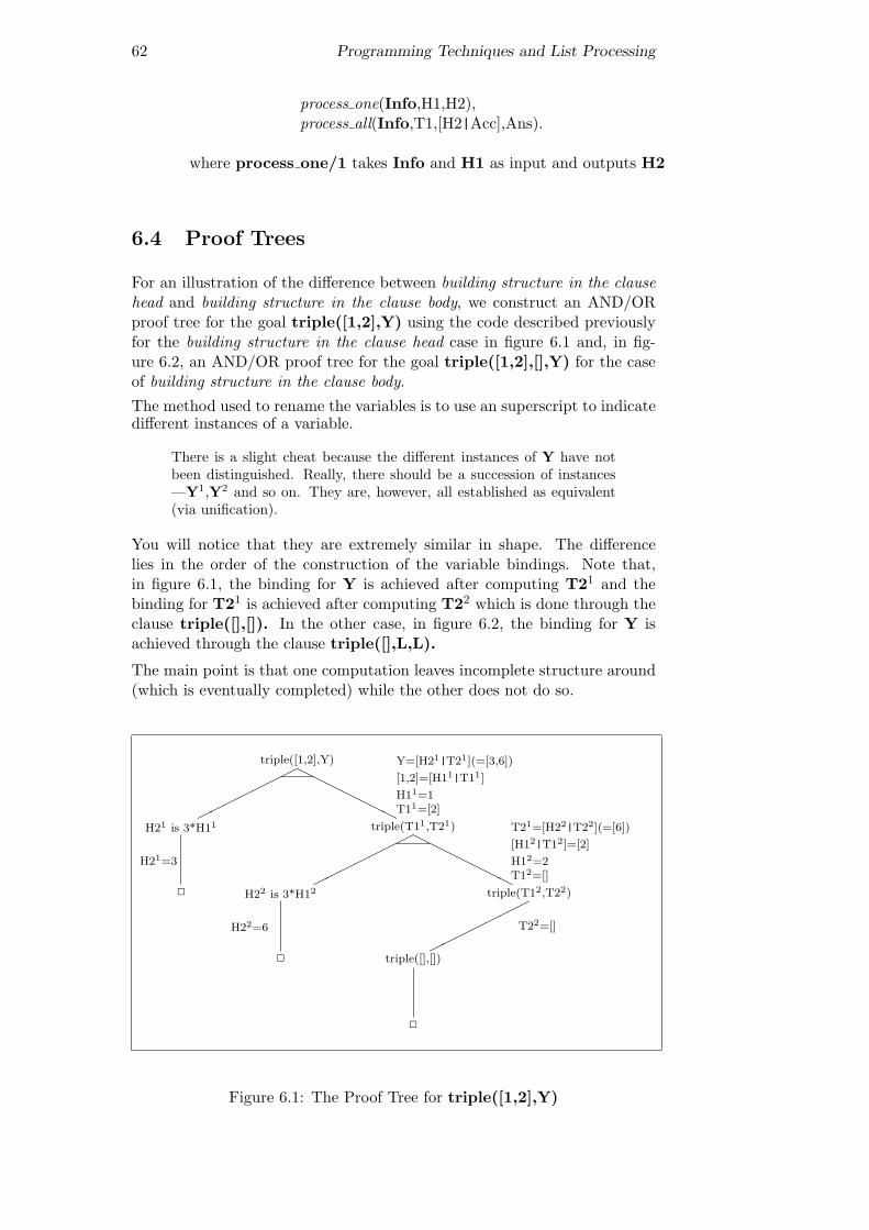
62 Programming Techniques and List Processing
process one(Info,H1,H2),process all(Info,T1,[H2|Acc],Ans).
where process one/1 takes Info and H1 as input and outputs H2
6.4 Proof Trees
For an illustration of the difference between building structure in the clausehead and building structure in the clause body, we construct an AND/ORproof tree for the goal triple([1,2],Y) using the code described previouslyfor the building structure in the clause head case in figure 6.1 and, in fig-ure 6.2, an AND/OR proof tree for the goal triple([1,2],[],Y) for the caseof building structure in the clause body.
The method used to rename the variables is to use an superscript to indicatedifferent instances of a variable.
There is a slight cheat because the different instances of Y have notbeen distinguished. Really, there should be a succession of instances—Y1,Y2 and so on. They are, however, all established as equivalent(via unification).
You will notice that they are extremely similar in shape. The differencelies in the order of the construction of the variable bindings. Note that,in figure 6.1, the binding for Y is achieved after computing T21 and thebinding for T21 is achieved after computing T22 which is done through theclause triple([],[]). In the other case, in figure 6.2, the binding for Y isachieved through the clause triple([],L,L).
The main point is that one computation leaves incomplete structure around(which is eventually completed) while the other does not do so.
triple([1,2],Y)HHHHHHH
©©©©©©©
Y=[H21|T21](=[3,6])
[1,2]=[H11|T11]
H11=1T11=[2]
H21 is 3*H11
2
triple(T11,T21)HHHHHHH
©©©©©©©
T21=[H22|T22](=[6])
[H12|T12]=[2]
H12=2T12=[]
H21=3
triple(T12,T22)©©©©©©©
H22 is 3*H12
2
T22=[]H22=6
triple([],[])
2
Figure 6.1: The Proof Tree for triple([1,2],Y)

63
triple([1,2],[],Y)HHHHHHH
©©©©©©©
[H11|T11]=[1,2]
H11=1T11=[2]
Acc1=[]
H21 is 3*H11
2
triple(T11,[H21|Acc1],Y)HHHHHHH
©©©©©©©
[H12|T12]=[2]
H12=2T12=[]
Acc2=[H21|Acc1](=[H21]=[3])H21=3
triple(T12,[H22|Acc2],Y)©©©©©©©
H22 is 3*H12
2
T22=[]
Acc3=[H22|Acc2](=[6,3])
H22=6
triple([],Acc3,Y)
2
Y=Acc3(=[6,3])
Figure 6.2: The Proof Tree for triple([1,2],[],Y)
6.5 What You Should Be Able To Do
After finishing the exercises at the end of the chapter:
You should be aware of some standard techniques for processinglists and be able to identify programs that use these techniques.
Exercise 6.1 We will now work on the four basic list schemata that wehave suggested:
1. The Schema test for existence
2. The Schema test all elements
3. The Schema return a result —having processed one element
4. The Schema return a result —having processed all elements
1. The Schema test for existence
(a) Define a predicate an integer/1 which checks to see if a list hasat least one integer in it. Use the built-in predicate integer/1.
?- an integer([a,fred,5,X]).yes
(b) Define a predicate has embedded lists/1 which checks to see ifa list is an element which is itself a list. Assume that the inputlist contains no variables and that the empty list is not a memberof this input list.
?- has embedded lists([a,[b],c,d,e]).yes

64 Programming Techniques and List Processing
2. The Schema test all elements
(a) Define a predicate all integers/1 that succeeds if and only if the(one) argument contains a list of integers.
?- all integers([1,fred,23]).no
(b) Define a predicate no consonants/1 which checks to see if a listof lower-case alphabetic characters has no consonants in it. Makeup your own predicate to check whether an atom is a consonant.
?- no consonants([a,e,i,t]).no?- no consonants([a,e,e,i]).yes
3. The Schema return a result —having processed one element
(a) Write a predicate nth/3 which takes two inputs: the first a posi-tive integer and the second a list. The output (initially, an unin-stantiated variable) will be the element that occurs at the nth po-sition in the list. So
?- nth(3,[this,is,[an,embedded,list]],X).X=[an,embedded,list]
(b) Define a predicate next/3 which again takes two inputs: a possi-ble member of a list and the list. The output should be the elementof the list that immediately follows the named list element (if itexists —if not, the predicate should fail).
?- next(a,[b,r,a,m,b,l,e],X).X=m
(c) define del 1st/3 which takes a possible element of a list and a listas inputs and ”returns” the list with the first occurence of thenamed element removed. (If the named element is not in the listthen the predicate is to fail)
?- del 1st(a,[b,a,n,a,n,a],X).X=[b,n,a,n,a]
This one can also be solved using an accumulator with the helpof append/3.
4. The Schema return a result —having processed all elements All thesecan be done in two ways. One uses the idea of building structure inthe clause head and the other building structure in the clause body.
Remember that the latter requires one more argument than the former—the accumulator. As this usually needs initialising it is customaryto do this by such as:

65
foo(a,X):-foo(a,[],X).
Do each problem both ways.
(a) Define nple/3 to take two inputs —an integer and a list of inte-gers. The result is to be a list of integers formed by multiplyingeach integer in the list by the input integer.
?- nple(5,[1,2,3],X).X=[5,10,15]
(b) Define del all/3 which takes a possible element of a list and alist as inputs and returns the list with all occurences of the namedelement removed. (If the named element is not in the list thenthe result is, of course, the whole list with no deletions)
?- del all(a,[b,a,n,a,n,a],X).X=[b,n,n]
(c) Define sum/2 to take a list of integers as input and return theoutput as their sum. This one is slightly unusual with regard tothe base case.
?- sum([1,32,3],X).X=36

Chapter 7
Control and Negation
negation-control
We introduce a number of facilities for controlling the executionof Prolog.We outline the problem of trying to represent logical negationand one solution.We introduce some more programming techniques.
7.1 Some Useful Predicates for Control
true/0
Always succeeds.
father(jim,fred).
is logically equivalent to
father(jim,fred):-true.
That is, any unit clause is equivalent to a non-unit clause with a singlesubgoal true in the body.
fail/0
Always fails.
lives forever(X):-fail.
is intended to mean that any attempt to solve the goal lives forever(X)will fail.
66

67
repeat/0
If it is asked to Redo then it will keep on succeeding.
test:-repeat,write(hello),fail.
The goal test produces the output:
hellohellohellohellohellohellohellohellohello...
repeat/0 behaves as if it were defined in Prolog as:
repeat.repeat:-
repeat.
call/1
The goal call(X) will call the interpreter as if the system were given thegoal X. Therefore X must be bound to a legal Prolog goal.
?- call(write(hello)).
helloyes
To handle a query which has multiple goals then:
?- call((write(hello),nl)).
helloyes
Note that we cannot write call(write(hello),nl) as this would betaken to be a usage of call/2 with the first argument write(hello)and the second argument nl) —and most systems do not have a call/2.
Note that call/1 is unusual in that its argument must be a legitimate Pro-log goal. Also note that call(X) will be legal if and only if X is bound toa legal goal.
7.2 The Problem of Negation
To maintain the connection with predicate logic, we would like to be ableto represent the negation of a statement. This, however, proves to be prob-lematic.
Consider

68 Control and Negation
man(jim).man(fred).
?- man(bert).
no
To say that man(bert) is not true we have to assume that we known allthat there is to know about man/1. The alternative is to say the the noindicates don’t know and this is not a possible truth value!
Turning to Prolog, If we try to solve a goal for which there is no clause (asin the case above) then we assume that we have provided Prolog with allthe necessary data to solve the problem. This is known as the Closed WorldAssumption.
This enables us to stick to the desirable property that a goal can have onlytwo outcomes.
\+/1
This strangely named predicate is Prolog’s equivalent to the not (oftenwritten as ¬ which stands for negation) of predicate logic. It is not namednot/1 because we it turns out that we cannot easily implement classicalnegation in Prolog.
The predicate \+/1 takes a Prolog goal as its argument. For example:
?- \+( man(jim) ).
will succeed if man(jim) fails and will fail if man(jim) succeeds.
7.2.1 Negation as Failure
Negation as failure is the term used to describe how we use the closed worldassumption to implement a form of negation in Prolog. We now give anexample which uses a rule to define women in terms of them not being men.Logically, ∀ x ∈ people ( ¬ man(x) =⇒ woman(x)).
man(jim).man(fred).woman(X):-
\+( man(X) ).
?- woman(jim).
no
The strategy is: to solve the goal woman(jim) try solving man(jim). Thissucceeds —therefore woman(jim) fails. Similarly, woman(jane) succeeds.But there is a problem. Consider:

69
?- woman(X).
It succeeds if man(X) fails —but man(X) succeeds with X bound to jim.So woman(X) fails and, because it fails, X cannot be bound to anything.
We can read ?- woman(X) as a query “is there a woman?” and thisquery failed. Yet we know that woman(jane) succeeds. Therefore,this form of negation is not at all like logical negation.The problem can be highlighted using predicate logic. The querywoman(X) is interpreted as
∃ x ¬ man(x)
which, logically, is equivalent to
¬ ∀ x man(x)
Now Prolog solves this goal in a manner roughly equivalent to
¬ ∃ x man(x)
The only time we get something like the desired result if there is noexistentially quantified variable in the goal. That is, whenever \+/1is used then make sure that its argument is bound at the time it iscalled.
Also, note that \+(\+(man(X))) is not identical to man(X) since theformer will succeed with X unbound while the latter will succeed with Xbound, in the first instance, to jim.
This is the basis of a well known Prolog programming ‘trick’ —i.e.it is a technique which is frowned upon by purists. The idea is totest whether, for example, two terms will unify without the effect ofbinding any variables. The goal \+(\+(X=2)) will succeed withoutbinding X to 2. The meaning is roughly X would unify with 2.
7.2.2 Using Negation in Case Selection
We can use \+/1 to define relations more carefully than previously. Toillustrate, consider
parity(X,odd):-odd(X).
parity(X,even).
together with the set of facts defining odd/1.
The goal parity(7,X) is intended to succeed using the first clause. Supposethat some later goal fails forcing backtracking to take place in such a waythat we try to redo parity(7,X). This goal unifies with the rest of thesecond clause! This is not desirable behaviour. We can fix this using \+/1.
parity(X,odd):-odd(X).
parity(X,even):-\+(odd(X)).

70 Control and Negation
Thus \+/1 provides extra expressivity as we do not need a set of facts todefine even/1.
If we go back to a previous example found in section 6.3.1 then we cannow resolve the problem about how to deal with unwanted backtrackingin programs like:
nested list([Head|Tail]):-sublist(Head).
nested list([Head|Tail]):-nested list(Tail).
sublist([]).sublist([Head|Tail]).
The problem is caused by the fact that a goal like nested list([a,[b],c,[d]])will succeed once and then, on redoing, will succeed once more. Thishappens because the goal unifies with the heads of both clauses —i.e.with nested list([Head|Tail]) (the heads are the same). We can nowstop this with the aid of \+/1:
nested list([Head|Tail]):-sublist(Head).
nested list([Head|Tail]):-\+(sublist(Head)),nested list(Tail).
sublist([]).sublist([Head|Tail]).
Note that this is at the price of often solving the identical subgoal twice—the repeated goal is sublist(Head). Note also that there is nevermore than one solution for sublist(X).Finally, we can define \+/1 using call/1 and the cut (!/0:
\+(X):-call(X),!,fail.
\+(X).
This is a definition which essentially states that “if X, interpreted asa goal, succeeds then \+(X) fails. If the goal X fails, then \+(X)succeeds. To see this is the case, you have to know the effect of thecut — fail combination ((!,fail). See later on in this chapter for moredetails of this.
7.3 Some General Program Schemata
We have already introduced some list processing schemata. Now we discusssome further, very general, program schemata.
Generate — Test
One of the most common techniques in Prolog is to use the backtracking infirst generating a possible solution, then testing the possible solution to seeif it is acceptable. If not, backtracking takes place so that another possiblesolution can be generated.

71
generate and test(Info,X):-. . .generate(Info,X),test(Info,X),. . .
In the above schema, the ellipsis (. . . ) indicates a number of subgoals (0 ormore).
We can distinguish two kinds of generator: a finite generator and an infinitegenerator. We will illustrate with two different versions of a non-negativeinteger generator which we will call int/1 —we cannot name this integer/1since this is already defined (as a built-in predicate) and it only works withmode integer(+) and we want int/1 to work with mode int(-).
Finite and Infinite Generators
We define a predicate integer with two digit square/1 to produce a pos-itive integer that has a square which is greater than or equal to 10 and lessthan 100.
integer with two digit square(X):-int(X),test square(X).
test square(X):-Y is X*X,Y >= 10,Y < 100.
Here is the definition of int/1 which is a finite generator —because thereare only a finite number of unit clauses (containing no variables) used todefine int/1.
int(1).int(2).int(3).int(4).int(5).
The goal integer with two digit square(X) eventually fails because thegenerator runs out of potential solutions. Now we define a version of int/1which is an infinite generator (verifying this is left as an ‘exercise for thereader’ !).
int(1).int(N):-
int(N1),N is N1 +1.

72 Control and Negation
On backtracking, this will generate a new solution for integer with two digit square(X)until we test 10. From then on, we will keep generating with int/1 and fail-ing with test square/1. We are trapped in a generate—test cycle with noway out.
The usual way out is to ensure that once we have found the solution wewant then we commit ourselves to that solution and forbid backtrackingfrom ever seeking another solution. Again, the usual solution is to placea cut (!/0) after the test. This results in:
integer with two digit square(X):-int(X),test square(X),!.
and the example demonstrates the (usually necessary) fix to stop a pro-gram using the generate — test schema from overgenerating. However,our solution now provides for only one solution to be generated!
Test — Process
Now we look at another fundamental schema. The idea with test — processis to guarantee that some inputs will only be ‘processed’ if the input passesa test.
test process(Info,X,Y):-test(Info,X),process(Info,X,Y).
where we assume that the Info is 0 or more arguments which are all inputarguments, the last but one argument is an input argument and the lastargument is a output argument. Although this gives a very procedural viewit is often possible to give a declarative reading.
We usually want to make sure that
1. test does not have alternative ways of confirming that the gener-ated element is ok
2. process does not have alternative ways of ‘processing’ the input
In short, we often want only one way of finding an output.
We have already met a program that satisfies this schema —one for parity/2(which is slightly rewritten here).
parity(X,Y):-odd(X),Y=odd.
parity(X,Y).\+(odd(X)),Y=even.
plus set of facts defining odd/1

73
This example illustrates that if the input argument is an integer then we seetwo cases: either the integer is even or it is odd. There is no third case. Norcan any integer be both even and odd.
As in the above example, the usage of test — process is closely coupled withthe idea of writing all the clauses for a predicate in this form —each clauseis designed to handle one ‘class’ of input. The whole scheme falls down ifwe do not design the ‘classes’ of input to be disjoint –i.e. no input falls intomore than one category. We also require that each input falls in at least onecategory —to summarise, each input falls in one and only one class.
We can show a previous example which does not properly use the test —process schema (for good reasons). Modifying the code using this schemaresults in a different and useful program.
member(Element,[Element|Tail]).member(Element,[Head|Tail]):-
member(Element,Tail).
Now member/2 can be used as a generator if the first argument is a variableand its second argument is a list —as in the goal member(X,[a,b,c,d,e,f ].The first solution for X is the first element of the list [a,b,c,d,e,f ]. Onredoing, we get, in succession, X bound to the different elements in the list.
We now rewrite using the test — process schema. We also rename thepredicate to the standard name of memberchk/2 (this is its usual namein libraries of Prolog code).
memberchk(Element,[Head|Tail]):-Element = Head.
memberchk(Element,[Head|Tail]):-\+(Element = Head),memberchk(Element,Tail).
This will no longer generate alternative solutions on backtracking for thegoal memberchk(X,[a,b,c,d,e,f ]) (because there are no alternative waysof resatisfying it). If the mode of use is mode memberchk(+,+) then themeaning is that we check that the first argument is an element of the list(which is the second argument).
Failure-Driven Loop
We now introduce an extremely procedural programming technique for sim-ulating a kind of iteration. The idea is deliberately generate a term andthen fail. This suggests the useless schema
failure driven loop(Info):-generate(Info,Term),fail.
failure driven loop(Info).

74 Control and Negation
Provided that the generator eventually fails any version of this schema willalways succeed —i.e. it will be equivalent to true.
We now use side effecting predicates to do something useful with the gener-ated term.
A side-effecting predicate is one that is (often) logically equivalent to truebut also does something else that is non-logical. For example, write/1 andnl/0 have the side-effect of writing material onto the terminal screen (usu-ally). Also, consult/1 and reconsult/1 have the side-effect of changing theprogram. The predicate read/1 has the side-effect of destructively readinginput from the terminal (or whatever).
To illustrate the problem: if we query Prolog with the goal(write(hello),fail) then write/1 will be used to write hello on (we as-sume) the terminal screen and the call to fail/0 will fail. Now, logically,we have a statement with the truth value of false —so we have proved thatthe goal cannot succeed and therefore there should be no message (hello)on the screen.
Here is another example: if we try the goal (read(X),fail) then read/1will be used to read some input from the user (we assume) and the call tofail/0 will fail. Again, we have a statement with the truth value of false—so the input should still be available for consideration. Yet we taken inputfrom the keyboard (or somewhere) and we do not put that input back sothat it can be reconsidered. The input has been consumed.
We can see that any predicate succeeds generating an effect that cannot beundone on backtracking must be a side-effecting predicate.
The complete failure-driven loop schema can be taken as:
failure driven loop(Info):-generate(Info,Term),side effect(Term),fail.
failure driven loop(Info).
This can be elaborated by having several side-effecting predicates, replacingthe fail/0 with some other predicate that fails and so on.
We illustrate with a simple example. We will use int/1 as a finite generatorand then print out the valid arguments for this relation on the screen.
int(1).int(2).int(3).int(4).int(5).
print int:-int(X),write(X),nl,fail.
print int.

75
This programming technique can be very useful. In the early days, it wasoverused because it was space-efficient.
Some Practical Problems
We now come to some needs that cannot easily be satisfied and still retaina clean declarative reading. We look at three problems that are intercon-nected.
Commit
We have outlined the use of test — process to do case analysis but it wasnecessary to have one clause for each case. If we have a goal which canbe satisfied via two different clauses then, on redoing, the same goal maygenerate a different solution.
In reality, this situation can arise quite often —i.e. the tests we do on theinput do not divide the input into non-overlapping classes. Essentially, wehave two problems. We often want to make sure that only one clause islegitimate —once it has been determined that the input passes some test.We think of this as a statement of commitment to the solution(s) derivedthrough ‘processing’ the input.
test process(Info,X,Y):-test(Info,X),commit,process(Info,X,Y).
When we backtrack and try to find another way of satisfying some programthat makes use of the test — process schema then we first try to find anotherway of satisfying the process part. If that fails, then we try to resatisfy thetest part. We do not want this to happen.
Then, assuming that we cannot resatisfy the test part, we try to resatisfythe goal making use of this program by trying different clauses.
Therefore there are two senses in which we may want to be ‘committed’: wewant to commit to using a single clause and we want to commit to the resultof a test —we do not want to run the risk that the test can be successful(with the same input) twice.
Satisfy Once Only
Sometimes, we would like a way of stopping Prolog looking for other solu-tions. That is, we want some predicate to have only one solution (if it hasone at all). This is the requirement that the predicate be determinate.
Naturally, predicates which do not have this property are indeterminate.This is a desirable property sometimes —e.g. the generate — test schemamakes use of the generator being indeterminate. On the other hand, itcan cause major problems when a program has many predicates which areunintentionally indeterminate. Our aim is to make sure that those predicateswhich should be determinate actually are determinate.

76 Control and Negation
We have already met an example of a predicate (memberchk/2) that mighthave been written with this situation in mind. We recall that member/2used with mode member(-,+) behaves as a generator. Perhaps it is worthpointing out that member/2 with mode member(+,+) is also, undercertain circumstances, resatisfiable —precisely when there are repetitions ofthe sought element in the list which constitutes the second argument.
Of course, if we are dealing with lists–as–sets, we should have arranged itso that the second argument does not have repeated elements. Anyway, itis very desirable to have a determinate version of member/2 available.
memberchk(X,[X|Y]):-make determinate.
memberchk(X,[Y|Z]):-memberchk(X,Z).
Note this isn’t quite what we had before. Previously, we arranged for mem-berchk/2 to be determinate with the help of \+/1. Stating our requirementas above, we seem to be going outside of logic in order to tell the Prologinterpreter that, once we have found the element sought, we never want toconsider this predicate as resatisfiable.
Fail Goal Now
We often search for the solution to a goal using several clauses for somepredicate. For example, we might have a social security calculation whichtries to assign how much money to give a claimant. Here is a fragment ofprogram:
calculate benefit(Claim Number,Nationality,Age,Other Details):-Nationality = british,calculate british entitlement(Age,Other Details).
calculate benefit(Claim Number,Nationality,Age,Other Details):-Nationality = martian,give up.
calculate benefit(Claim Number,Nationality,Age,Other Details):-Nationality = french,calculate french entitlement(Age,Other Details).
If we reach the situation where we realise that the whole search is doomedthen we may want to say something informally like ‘stop this line of approachto the solution and any other corresponding line’. In the above, if we findwe are trying to assign benefit to a martian then we make the decisionthat calculate benefit/4 should fail and therefore that there is no pointin trying to use any remaining clauses to find a solution.
In practice, we need to make use of this kind of action. Again, we arepotentially asking Prolog to behave abnormally.
In fact, in all these situations, we are asking Prolog to behave in a non-standard way. Whatever the complications, it is hard top make do withoutways to:

77
• Commit
• Make Determinate
• Fail Goal Now
7.4 What You Should Be Able To Do
You should be able to make use of the ‘predicates’ true/0,fail/0, repeat/0 and call/1.You should be able to describe the difference between the openand closed world assumptions.You should be able to describe the difference between classicalnegation and negation as failure.You should be able to distinguish side-effecting from non side-effecting predicates.You should be able to use Prolog negation to achieve theeffect of case selection.You should be able to use the techniques of generate — test,test — process and failure-driven loop. You should also beaware of the needs for the techniques commit — process,satisfy–only–once and fail–goal–now.

Chapter 8
Parsing in Prolog
parsing-chap
We introduce the facilities that Prolog provides for parsing.This is done through the idea of a parse tree as applied to asimple model for the construction of English sentences.Three ways of parsing Prolog are described: the first illustratesthe ideas, the second is more efficient and the third providesan easy way of coding a parser via Grammar Rules.We then explain how to extract the parse tree and show howto extend a parser using arbitrary Prolog code.
Later on in the course, you will be involved in trying to face up to theproblem of parsing ordinary english language sentences. For this lecture,we shall also be interested in parsing sentences but we will look at the verysimplest examples.
First, what do we want the parser to do? We would like to know that asentence is correct according to the (recognised) laws of english grammar.
The ball runs fast
is syntactically correct while
The man goes pub
is not as the verb “go” (usually) does not take a direct object.
Secondly, we may want to build up some structure which describes thesentence —so it would be worth returning, as a result of the parse, anexpression which represents the syntactic structure of the successfully parsedsentence.
Of course, we are not going to try to extract the meaning of the sentenceso we will not consider attempting to build any semantic structures.
8.1 Simple English Syntax
The components of this simple syntax will be such categories as sentences,nouns, verbs etc. Here is a (top down) description:
78

79
Unit: sentenceConstructed from: noun phrase followed by a verb phrase
Unit: noun phraseConstructed from: proper noun or determiner followed by a noun
Unit: verb phraseConstructed from: verb or verb followed by noun phrase
Unit: determinerExamples: a, the
Unit: nounExamples: man, cake
Unit verb:Examples: ate
8.2 The Parse Tree
Figure 8.1 shows the parse tree for the sentence:
the man ate the cake
with some common abbreviations in brackets. We must remember that
sentence(s)
nounphrase(np)
ÃÃÃÃÃÃÃÃ
verbphrase(vp)
```````
determiner(det)
»»»»»»
noun
HHHnounphrase
(np)
XXXXXX
verb
»»»»»»
the man atedeterminer
(det)
»»»»»»
noun
HHH
the cake
Figure 8.1: A Parse Tree
many sentences are ambiguous —i.e. they result in different parse trees.

80 Parsing in Prolog
8.3 First Attempt at Parsing
We assume that we will parse sentences converted to list format. Thatis, the sentence “the man ate the cake” will be represented by the list[the,man,ate,the,cake].
We use append/3 to glue two lists together. The idea is that append/3returns the result of gluing takes input as lists in the first and second argu-ment positions and returns the result in the third position.
sentence(S):-append(NP,VP,S),noun phrase(NP),verb phrase(VP).
noun phrase(NP):-append(Det,Noun,NP),determiner(Det),noun(Noun).
verb phrase(VP):-append(Verb,NP,VP),verb(Verb),noun phrase(NP).
determiner([a]).determiner([the]).noun([man]).noun([cake]).verb([ate]).
Here is what happens to the query:
?- sentence([the,man,ate,the cake]).
append/3 succeeds with NP=[], VP=[the,man,ate,the,cake]noun phrase/1 failsappend/3 succeeds with NP=[the], VP=[man,ate,the,cake]noun phrase/1 failsappend/3 succeeds with NP=[the,man], VP=[ate,the,cake]noun phrase/1 succeeds. . .verb phrase/1 succeeds
This is all very well but the process of parsing with this method is heavilynon deterministic.
Also, it suffers from not being a very flexible way of expressing some situa-tions. For example, the problem of adjectives:
the quick fox
81
is also a noun phrase.
We might try to parse this kind of noun phrase with the extra clause:
noun phrase(NP):-append(Det,Bit,NP),determiner(Det),append(Adj,Noun,Bit),adjective(Adj),noun(Noun).
A little ungainly.
8.4 A Second Approach
We now try an approach which is less non-deterministic. We will start bylooking at:
sentence(In,Out)
The idea is that sentence/2 takes in a list of words as input, finds a legalsentence and returns a result consisting of the input list minus all the wordsthat formed the legal sentence.
We can define it:
sentence(S,S0):-noun phrase(S,S1),verb phrase(S1,S0).
Here is a rough semantics for sentence/2.
A sentence can be found at the front of a list of words if there is anoun phrase at the front of the list and a verb phrase immediatelyfollowing.
This declarative reading should help to bridge the gap between what wewant to be a sentence and the procedure for finding a sentence.
Here is the rest of the parser:
noun phrase(NP,NP0):-determiner(NP,NP1),noun(NP1,NP0).
verb phrase(VP,VP0):-verb(VP,VP1),noun phrase(VP1,VP0).
determiner([a|Rest],Rest).determiner([the|Rest],Rest).noun([man|Rest],Rest).noun([cake|Rest],Rest).verb([ate|Rest],Rest).

82 Parsing in Prolog
As you can see, there is a remarkable sameness about each rule which, onceyou see what is going on, is fairly tedious to type in every time. So we turnto a facility that is built in to Prolog.
8.5 Prolog Grammar Rules
Prolog, as a convenience, will do most of the tedious work for you. Whatfollows, is the way you can take advantage of Prolog.
This is how we can define the simple grammar which is accepted ‘as is’ byProlog.
sentence --> noun phrase, verb phrase.noun phrase --> determiner, noun.verb phrase --> verb, noun phrase.determiner --> [a].determiner --> [the].noun --> [man].noun --> [cake].verb --> [ate].
It is very easy to extend if we want to include adjectives.
noun phrase --> determiner, adjectives, noun.adjectives --> adjective.adjectives --> adjective, adjectives.adjective --> [young].
This formulation is sometimes known as a Definite Clause Grammar (DCG).
We might later think about the ordering of these rules and whether theyreally capture the way we use adjectives in general conversation but notnow.
Essentially, the Prolog Grammar Rule formulation is syntactic sugaring.This means that Prolog enables you to write in:
sentence --> noun phrase, verb phrase.
and Prolog turns this into:
sentence(S,S0):-noun phrase(S,S1),verb phrase(S1,S0).
and
adjective --> [young].
into

83
adjective(A,A0):-’C’(A,young,A0).
where ’C’/3 is a built in Prolog Predicate which is defined as if:
’C’([H|T],H,T).
8.6 To Use the Grammar Rules
Set a goal of the form
sentence([the,man,ate,a,cake],[])
and not as
sentence.
or
sentence([the,man,ate,a,cake])
8.7 How to Extract a Parse Tree
We can add an extra argument which can be used to return a result.
sentence([[np,NP],[vp,VP]]) --> noun phrase(NP), verb phrase(VP).noun phrase([[det,Det],[noun,Noun]]) --> determiner(Det), noun(Noun).determiner(the) --> [the].and so on
What we have done above is declare predicates sentence/3,noun phrase/3, verb phrase/3, determiner/3 and so on. The explicitargument is the first and the two others are added when the clause is readin by Prolog. Basically, Prolog expands a grammar rule with n argumentsinto a corresponding clause with n+2 arguments.
So what structure is returned from solving the goal:
sentence(Structure,[the,man,ate,a,cake],[])
The result is:
[[np,[[det,the],[noun,man]]],[vp,[...
Not too easy to read!

84 Parsing in Prolog
We can improve on this representation if we are allowed to use Prologterms as arguments. For example, in foo(happy(fred),12) the termhappy(fred) is one of the arguments of foo/2. Such a term is knownas a compound term. We discuss this at greater length in chapter ??.With the help of compound terms, we could tidy up our representationof sentence structure to something akin to:
sentence([np([det(the),noun(man)]),vp([...
8.8 Adding Arbitrary Prolog Goals
Grammar rules are simply expanded to Prolog goals. We can also insertarbitrary Prolog subgoals on the right hand side of a grammar rule butwe must tell Prolog that we do not want them expanded. This is donewith the help of braces —i.e. { }. For example, here is a grammar rulewhich parses a single character input as an ASCII code and succeeds if thecharacter represents a digit. It also returns the digit found.
digit(D) -->[X],{ X >= 48,
X =< 57,D is X-48 }.
The grammar rule looks for a character at the head of a list of input char-acters and succeeds if the Prolog subgoals
{ X >= 48,X =< 57,D is X-48 }.
succeed. Note that we assume we are working with ASCII codes for thecharacters and that the ASCII code for “0” is 48 and for “9” is 57. Alsonote the strange way of signifying “equal to or less than” as “=<”.
8.9 What You Should Be Able To Do
After finishing the exercises at the end of the chapter:
You should be able to write a simple parser for a small subsetof English.You should be able to use Prolog’s grammar rules to definethe grammar of a simple language.You should be able to describe how Prolog rewrites the gram-mar rules into ‘standard’ Prolog.You should be able to use the grammar rules to extract a parsetree.
Exercise 8.1 Here is a Definite Clause Grammar:

85
s --> np,vp.np --> det,noun.np --> det,adjs,noun.vp --> verb,np.det --> [a].det --> [the].adjs --> adj.adjs --> adj,adjs.adj --> [clever].noun --> [boy].noun --> [sweet].verb --> [buys].
1. Give some examples of sentences that this grammar could parse.
2. Modify this DCG so that the parse returns information about the struc-ture of the sentence.
3. Suppose that the DCG is given a sentence to parse containing a mis-spelled word -say “boy”. Modify the DCG so that the information aboutthe structure of the sentence will include some information about anyunrecognised component.
4. Suppose now that the DCG is given a sentence to parse missing a wordor two. Modify the DCG so that it will identify the missing component.
The last two parts of this exercise are hard —it is essentially the problem ofrobust parsing. We try to do the best we can to identify gaps, misspellingsand redundant information.

Chapter 9
Modifying the Search Space
extralogical
We describe solutions to various problems of control raised inchapter ??.We detail other useful Prolog built-in predicates that are non-logical.
9.1 A Special Control Predicate
We now present a solution to the practical problems posed in chapter ??about how to control Prolog’s search strategy. We summarised these issuesas ones of:
• Commit
• Make Determinate
• Fail Goal Now
In each of these cases the solution is to make use of a built-in predicate whichalways succeeds —but with a very unpleasant side-effect. This notoriouspredicate is known as the cut and written !/0.
The reason why cut (!/0) is so unpleasant are that it effects Prolog’s searchtree. Consequently, by adding a cut, the program’s meaning may changeradically. We sometimes say that a cut that does this is a red cut. On theother hand, the placing of a cut may not change the intended meaning butsimply junk a part of the search tree where it is known that there is no legalsolution. Such a cut is termed a green cut. The Art of Prolog by Sterlingand Shapiro has a nice section on the cut [Sterling & Shapiro, 1986].
We now go over how to solve the three control problems.
9.1.1 Commit
Assume we want to make Social Security payments. That is, pay(X,Y)means “pay the sum X to Y”. Assume that we also have this code fragment.
86

87
pay(X,Y):-british(X),entitled(X,Details,Y).
pay(X,Y):-european(X),entitled(X,Details,Y).
In each clause, the first subgoal in the body is acting as a test in a programusing the test — process schema. We also assume that, for some reason,we have not been able to apply the disjoint (and exhaustive) case analysistechnique.
Consequently, if we have successfully checked that a person is British and,for some reason, the subgoal entitled(X,Details,Y) fails (or some latercomputation forces backtracking back to redo the call to pay/2 that weare considering) then there may be no point in
• checking if they are “european” (assuming that there are no regulationsunder which British people can qualify for payment as being Europeanwhen they fail to qualify as British citizens).
• checking to see if there is more than one entry for the person in somedatabase accessed by british/1.
In the immediate situation, we want to be committed to telling Prolog notto redo the british/1 subgoal and not to consider other clauses for pay/2that might contribute an alternative.
The truth is, of course, that we may want these two consequences whetheror not entitled/3 fails.
If this is so, then we insert a cut as shown below and highlighted by a box .
pay(X,Y):-british(X),! ,entitled(X,Details,Y).
pay(X,Y):-european(X),! ,entitled(X,Details,Y).
We want to be committed to the choice for the pay/2 predicate. We cansee the use of !/0 as a guard that has two effects.
• On backtracking through the list of subgoals: a cut can be thought ofas indicating that all attempts to redo a subgoal to the left of the cutresults in the subgoal immediately failing. We sometimes say that anyunifications taking place prior to the cut have been frozen and cannotbe remade.
• On backtracking into the predicate once the call had exited: if one ofthe clauses defining the predicate had previously contained a cut that

88 Modifying the Search Space
had been executed then no other clauses for that predicate may be usedto resatisfy the goal being redone. We sometimes say that, once a cutis executed, later clauses have been chopped out of the search space.
Note that, with the cut in the position it is above, it is still possible thatentitled/3 could be resatisfied. We have to guarantee that we have madeentitled/3 determinate before we can guarantee that pay/2 is determinate.We have to do some more on this issue.
Also note that the effect of cut (!/0) prunes the search space only until theparent goal of the cut fails. If we leave the Fail port of pay/2 and someprevious goal leads to another call to pay/2 then the cut (!/0) has no effectuntil it is executed.
We also have to remember that cut (!/0) has two distinct effects: back-tracking cannot redo any subgoals to the left of the cut and clauses in theprogram database for the same predicate that are textually after the currentclause are unreachable. See figure 9.1 for a graphic representation of theseeffects on a rather artificial program.
a(X):- b(X),c(X).b(1).b(4).c(X):- d(X),!,e(X).c(X):- f(X).d(X):- g(X).d(X):- h(X).e(3).f(4).g(2).h(1).
a(X)©©©©©©©
XXXXXXXXXXXXXXb(X)
2
X=1
d(1)©©©©©©©
g(1)
HHHHHHHh(1)
2
Frozen
©©©©©©©©©©
HHHHHHHHHH
c(X)»»»»»»»»»»»»»»
©©©©©©©
XXXXXXXXXXXXXX! e(X) f(X)
Chopped
Figure 9.1: The Effect of cut on the AND/OR Tree

89
9.1.2 Make Determinate
We now go onto the key problem of making our programs determinate. Thatis, if they succeed, then they succeed precisely once unless we really wantthem to generate alternative solutions. Many programmers find tamingbacktracking to be a major problem.
Consider the problem raised by this program:
sum(1,1).sum(N,Ans):-
NewN is N-1,sum(NewN,Ans1),Ans is Ans1+N.
together with the goal
?- sum(2,X).
The meaning of sum/2 is that, for the first argument N (a positive integer),there is some integer, the second argument, which is the sum of the first Npositive integers.
We know that, for the mode sum(+,-), there is only one such result.Therefore, if we try to redo a goal such as sum(2,Ans) it should fail. Wecould test that this is so with:
?- sum(2,Ans),write(Ans),nl,fail.
We would like the result:
3no
Alas, here is the result using Edinburgh Prolog.
3(a very very long wait)
We have a runaway recursion. Figure 9.2 shows the execution tree for thegoal sum(2,Ans). Now look at the goal:
?- sum(2,X),fail.
and the resulting fragment of the execution tree which is shown in figure 9.3.Prolog goes into a non terminating computation. We want to make surethat, having found a solution, Prolog never looks for another solution viaRedoing the goal. Figure 9.4 shows the consequence when the cut (!/0) isused.

90 Modifying the Search Space
sum(2,Ans1)
@@
@@
@@
@@
¡¡
¡¡
¡¡
¡¡
©©©©©©©©©©©©©©©©
©©©©©©©©©©©©©©©©
2
2 2
sum(NewN1,Ans11) Ans1 is Ans11+2
Ans1=3
NewN1 is 2-1
NewN1=1
sum(1,1)
Ans11=1
sum(1,1)
Figure 9.2: The First Solution to the Goal sum(2,Ans)
sum(1,1):-! .
sum(N,Ans):-NewN is N-1,sum(NewN,Ans1),Ans is Ans1+N.
9.1.3 Fail Goal Now
We are trying to solve the problem that arises when we realise, in the middleof satisfying subgoals for some goal, that the goal will never succeed —evenif we try other clauses which have heads that unify with the goal.
Here is a way of defining woman/1 in terms of man/1 where we base theidea that, in trying to establish that someone is a “woman”, we prove thatthey are actually a “man” and there is therefore no point in trying to findsome other proof that this person is a woman.
woman(X):-man(X),! ,fail.
woman(X).

91
sum(2,Ans1)
@@
@@
@@
@@
¡¡
¡¡
¡¡
¡¡
@@
@@
@@
@
¡¡
¡¡
¡¡
¡
©©©©©©©©©©©©©©©¼
@@
@@
@@
@@
¡¡
¡¡
¡¡
¡¡
©©©©©©©©©©©©©©©©
©©©©©©©©©©©©©©©©
2
2
sum(NewN1,Ans11)
sum(NewN2,Ans12)Ans11 is Ans12+NewN1
Ans1 is Ans11+2
Ans1 6=3
NewN1 is 2-1
NewN1=1
NewN2 is N2-1
NewN2=0
sum(1,1)
Ans11 6=1
sum(1,1)
Figure 9.3: Resatisfying the Goal sum(2,Ans)
Putting it a slightly different way, to solve for woman(jim) we tryman(jim). If that succeeds then we want to abandon the attempt to provewoman(jim) without trying any other clauses for woman/1.
Note that the use of the cut (!/0) stops any attempt to resatisfy man/1once backtracking is forced through fail/1 failing. Note also that the secondclause for woman/1 will not be used after the cut—fail combination hasbeen met.
We call this use of cut in conjunction with fail/0 the cut—fail technique.
The above code for woman/1 is a special case of Prolog’s implementationof negation as failure. Here is a possible definition of \+/1 using cut (!/0)and call/1.
\+(Goal):-call(Goal),!,fail.
\+(Goal).
9.2 Changing the Program
The use of cut (!/0) changes the search space while the program is run-ning. We now introduce a family of predicates that can be used to changethe search space during program execution. We do this with the strongestrequest:
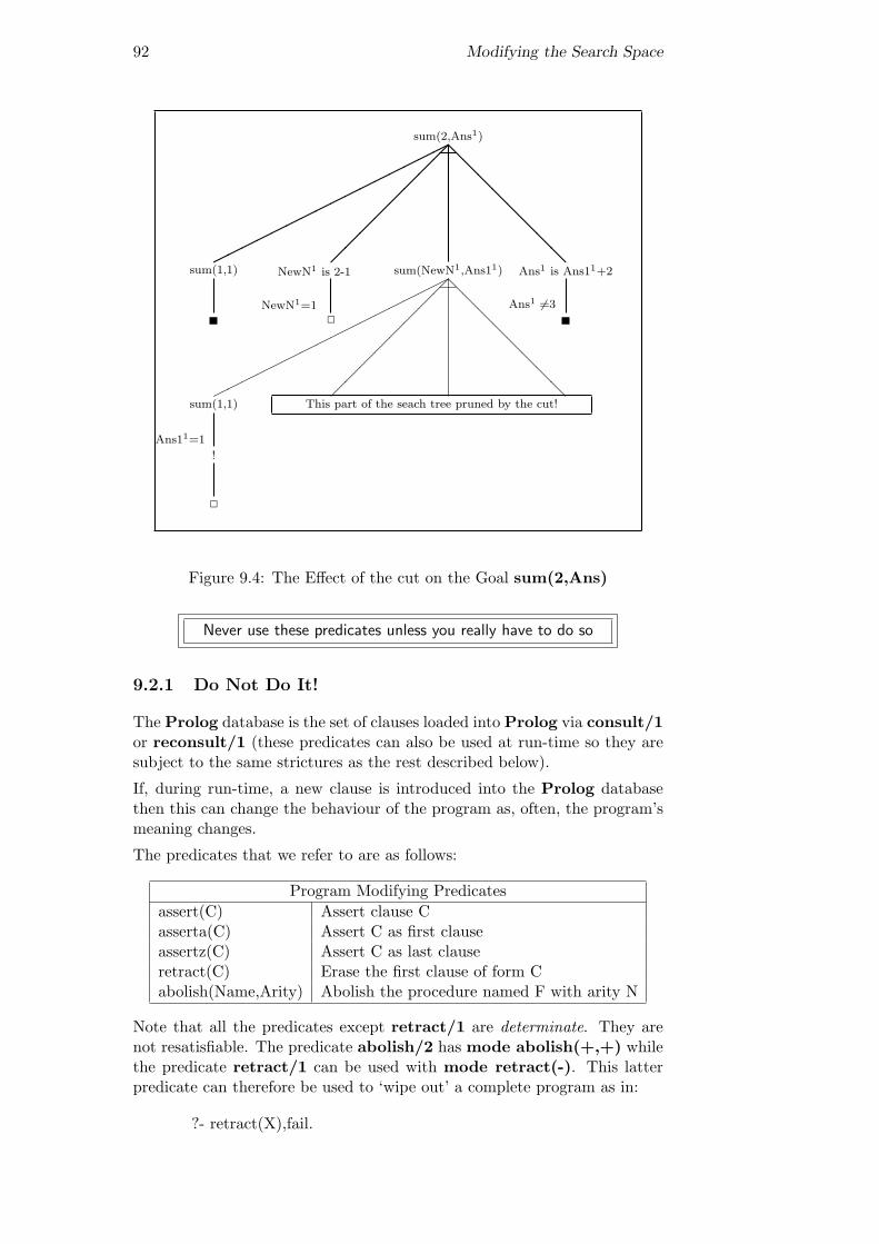
92 Modifying the Search Space
sum(2,Ans1)
@@
@@
@@
@@
¡¡
¡¡
¡¡
¡¡
@@
@@
@@
@@
¡¡
¡¡
¡¡
¡¡
©©©©©©©©©©©©©©©©
©©©©©©©©©©©©©©©©
!
2
2
sum(NewN1,Ans11) Ans1 is Ans11+2
Ans1 6=3
NewN1 is 2-1
NewN1=1
sum(1,1)
Ans11=1
sum(1,1)
This part of the seach tree pruned by the cut!
Figure 9.4: The Effect of the cut on the Goal sum(2,Ans)
Never use these predicates unless you really have to do so
9.2.1 Do Not Do It!
The Prolog database is the set of clauses loaded into Prolog via consult/1or reconsult/1 (these predicates can also be used at run-time so they aresubject to the same strictures as the rest described below).
If, during run-time, a new clause is introduced into the Prolog databasethen this can change the behaviour of the program as, often, the program’smeaning changes.
The predicates that we refer to are as follows:
Program Modifying Predicatesassert(C) Assert clause Casserta(C) Assert C as first clauseassertz(C) Assert C as last clauseretract(C) Erase the first clause of form Cabolish(Name,Arity) Abolish the procedure named F with arity N
Note that all the predicates except retract/1 are determinate. They arenot resatisfiable. The predicate abolish/2 has mode abolish(+,+) whilethe predicate retract/1 can be used with mode retract(-). This latterpredicate can therefore be used to ‘wipe out’ a complete program as in:
?- retract(X),fail.

93
This will fail with the side-effect of removing all the clauses loaded. We canremove just some clauses as in:
?- retract(foo(1,X)).
will remove all clauses whose heads unify with foo(1,X).
Note that to add a clause which is also a rule you will need to writeassert((a:- b)) and not assert(a:-b). See chapter ?? for an explanation.
Together, these predicates can be used to implement global flags and aform of global variable. This almost always makes it harder to understandindividual parts of the program —let alone the disastrous effect such changeshave on the declarative reading of programs.
All these predicates are side-effect ing. Therefore, backtracking will not undothese side-effects. For example, if assert/1 is used to maintain a databaseof results found so far then, on backtracking, Prolog will not remove theseresults.
Further, the program becomes sensitive to interupts. It has been known forsomeone to abort a program (using ^C and then a for abort) between theasserting of a new clause and the retracting of an old clause —leaving anunexpected old clause around which interfered badly with the subsequentexecution of the program.
If a problem seems to require the use of assert/1 then, usually, there isanother way of doing things.
9.2.2 Sometimes You have To!
There are one or two occasions when you might want to use these predicates.The main one is when you have definitely proved that something is the case.That is, there is no way in which some statement (added to the programas a clause) can be false. Sometimes, of course, a program is supposed tomodify the Prolog database. For example, consult/1 and reconsult/1.
Often, we do not want to modify the program itself —rather, we want tochange the data the program accesses. There is a facility in EdinburghProlog known as the recorded database. This is a way of storing Prologterms under a key. Such terms are hidden from the listing/0 program. Thepredicates that access this recorded database are:
Program Modifying Predicateserase(R) Erase the record with reference R.record(K,T,R) Record term T under key K, reference R.recorda(K,T,R) Make term T the first record under key K, reference R.recorded(K,T,R) Term T is recorded under key K, reference R.recordz(K,T,R) Make term T the last record under key K, reference R.
These can be used to squirrel away information to be used by the programitself. An example is the predicate random/2:
random(Range,Num):- % to choose random number in rangerecorded(seed,Seed,Ref), % get seed from database

94 Modifying the Search Space
erase(Ref), % delete old value of seedNum is (Seed mod Range) + 1, % fit seed into rangeNewSeed is (125*Seed+1) mod 4093,% calculate new valuerecord(seed,NewSeed, Ref). % and assert it into database
This shows how we can maintain information about the seed used to generatethe next pseudo-random number. Note that, unless we want to delete anentry (using erase/1) we usually use an anonymous variable for the recordreference.
Using this family of predicates is more elegant (and sometimes more efficient)but suffers from the same problems as the assert family.
9.3 What You Should Be Able To Do
After finishing the exercises at the end of the chapter:
You should be able to use the cut (!) to implement thetechniques of commit, make–determinate and fail–goal–now(cut—fail).You should know how to change the program at run-time andunderstand the dangers in doing so. You should know some ofthe circumstances when it is acceptable to do so.You should know how to use the recorded database.
Exercise 9.1 1. Given the following clauses, it is required to place cut(s)in the program to achieve the given outputs: First, determine what theoutput will be without placing any cuts in the program.
female author:-author(X),write(X),write(’ is an author’),nl,female(X),write(’ and female’),nl.
female author:-write(’no luck!’),nl.
author(X):-name(X).
author(X):-write(’no more found!’),nl,fail.
name(sartre).name(calvino).name(joyce).

95
female(murdoch).female(bembridge).
and here are the desired outputs. Make sure that you use only one cutto get the desired output.
(a) sartre is an authorno more found!no luck!
(b) sartre is an authorcalvino is an authorjoyce is an authorno more found!
(c) sartre is an authorno luck!
(d) sartre is an author
(e) sartre is an authorcalvino is an authorjoyce is an authorno luck!
2. Here is an example of code taken from one of the standard Prologlibraries —only all the cuts have been removed! Try to put them back.
delete([], , []).delete([Kill|Tail], Kill, Rest) :-
delete(Tail, Kill, Rest).delete([Head|Tail], Kill, [Head|Rest]):-
delete(Tail, Kill, Rest).
The semantics is roughly “remove the element named in the secondargument from the list in the first argument to produce the list in thethird argument (which does not contain any copies of the element tobe removed)”.
Therefore, the first two arguments are supposed to be inputs and thethird an output. Note that the predicate must be determinate so that,if asked to Redo, it will fail.
3. Define a predicate disjoint/1 which is true only when the argumentto disjoint/1 contains no repeated elements. Make sure that the pred-icate is determinate.
Now use the cut—fail method to define the same predicate.

96 Modifying the Search Space
4. Try writing plus/3 which declares that “the first two arguments addup to the third argument provided all the instantiated arguments areintegers”. If, however, less than two argument are not integers thenthe predicate should fail and print out some pleasing error message.
Note that this is not equivalent to “Z is X + Y” and get the cuts in!

Chapter 10
Prolog Syntax
syntax
We describe Prolog syntax more formally.We introduce the concept of a Prolog term, a variation of thelogical variable and arbitrarily nested terms.We explain how two Prolog terms are unified and demonstratethe need for a special check to ensure that we do not get infinitedatastructures.We show that lists are also terms and illustrate how to con-catenate two lists together.We also show that the structure of every Prolog clause is alsoa Prolog term.
Prolog Terms are one of:
• Constant
• Variable
• Compound Term
10.1 Constants
A Constant is one of:
• Atom
• Integer
• Real Number
Atoms are made up of:
• letters and digits: AB...Zab...z01...9 and (underscore)
• symbol: any number of +, -, *, /, \, ^, <, >, =, ~, :, ., ?, @, #, $ &
• quoted strings: ’any old character’ —but the single quote character ishandled specially
Normally, atoms start with a lower case letter. Note that, in a quoted atom,you can include a “ ’ ” by prefixing it with another “ ’ ”. So, to print a “ ’ ”on the screen you will need a goal like write(’ ’ ’ ’).
97

98 Prolog Syntax
10.2 Variables
Variables usually start with a capital letter. The only interesting exceptionis the special anonymous variable written and pronounced “underscore”.In the rule
process(X,Y):-generate( ,Z),test( ,Z),evaluate(Z,Y).
the underscores refer to different unnamed variables. For example, here aretwo versions of member/2.
member(X,[X|Y]).member(X,[Y|Z]):-
member(X,Z).
member(X,[X| ]).member(X,[ |Z]):-
member(X,Z).
Note that, in the clause,
know both parents(X):-mother( ,X),father( ,X).
the underscores do not refer to the same object. The reading is roughlythat “we know both the parents of X if someone(name unimportant) is themother of X and someone else (unimportant) is the father”. Note thatProlog regards the two occurrences of the anonymous variable in the aboveas different variables.
10.3 Compound Terms
A Compound Term is a functor with a (fixed) number of arguments each ofwhich may be a Prolog term.
This means that we can arbitrarily nest compound terms. For some exam-ples:
happy(fred)principal functor = happy1st argument = a constant (atom)
sum(5,X)principal functor = sum1st argument = constant (integer)

99
2nd argument = variable
not(happy(woman))principal functor = not1st argument = compound term
Nesting compound terms may be of use to the programmer. For example,the clause
fact(fred,10000).
is not as informative as
fact(name(fred),salary(10000)).
which can be thought of as defining a PASCAL-type record structure.
10.4 (Compound) Terms as Trees
Take the compound term
sentence(np(noun(fred)),vp(verb(swims)))
and construct a tree. Start by marking the root of the tree with the principalfunctor and draw as many arcs as the principle functor has arguments. Foreach of the arguments, repeat the above procedure.
sentence!!!!!!
aaaaaanp vp
noun verb
fred swims
10.5 Compound Terms and Unification
Consider
?- happy(X)=sad(jim).
—fails, because we know that it is necessary that the principal functors andtheir arities are the same for unification to succeed.

100 Prolog Syntax
?- data(X,salary(10000))=data(name(fred),Y).
—succeeds, because, having matched the principal functors (and checkedthat the arities are the same) we recursively try to match correspondingarguments. This generates two subgoals:
X = name(fred)salary(10000) = Y
which both succeed.
10.6 The Occurs Check
This is an aside. If we try to unify two expressions we must generally avoidsituations where the unification process tries to build infinite structures.Consider:
data(X,name(X)).
and try:
?- data(Y,Y).
First we successfully match the first arguments and Y is bound to X. Nowwe try to match Y with name(X). This involves trying to unify name(X)with X. What happens is an attempt to identify X with name(X) whichyields a new problem —to match name(X) against name(name(X)) and soon. We get a form of circularity which most Prolog systems cannot handle.
To avoid this it is necessary, that, whenever an attempt is made to unify avariable with a compound term, we check to see if the variable is containedwithin the structure of the compound term.
This check is known as the occurs check. If we try to unify two terms andwe end up trying to unify a variable against a term containing that variablethen the unification should fail.
Most Prolog implementations have deliberately missed out the occurs check—mostly because it is computationally very expensive.
Consequently, the goal X=f(X) will usually succeed where it should reallyfail. The most common way in which this error might manifest itself is whenthe system tries to print out the binding for X. This usually results in anattempt to print an infinite term.
?- X=f(X).X=f(f(f(f(f(f(f(f(f(f(f(f(f(f(f...

101
10.7 Lists Are Terms Too
If a list is a term then it must be a compound term. What, then is itsprincipal functor? Predicates have a fixed arity but lists can be any length—so what is the arity of the principle functor?
For the moment only, let us suppose we have a gluing agent which glues anelement onto the front of a list. We know this is a reasonable suppositionbecause we already have a list destructor/constructor that works like this.
[a,b,c,d] = [Head|Tail]—results in Head=a, Tail=[b,c,d]
We might think of this constructor as a predicate cons/2. We have to buildlists like this. Note, however, that there is no built-in predicate namedcons/2 —the real name for the list constructor function is ./2!
In Prolog, the empty list is represented as []. In some implementations, theempty list is named “nil” —but the Prolog you will use does not use thisname.
Familiar Intermediate Compound TermList Notation Form Form[ ] [][a] cons(a,[])[b,a] cons(b,[a]) cons(b,cons(a,[]))[c,b,a] cons(c,[b,a]) cons(c,cons(b,cons(a,[])))
Now to represent the lists as trees —but we will distort them a little:
r []
[]
r []
[a]
a
r r []
[a,b]
b a
You will have noticed that we could have written cons where we have writ-ten . —well, remember that Prolog doesn’t use a meaningful name for theconstructor cons/2. Really, the constructor is ./2. For (textual) explana-tion purposes, we shall stick to using cons/2.
Now we will show how to unpack the structure of a non-flat list. We do thisby building up the structure from left to right.
[a,[b,c],d]goes to
cons(a,[[b,c],d])goes to
cons(a,cons([b,c],[d])goes to
now [b,c] is cons(b,[c])

102 Prolog Syntax
that is, cons(b,cons(c,[]))cons(a,cons(cons(b,cons(c,[])),[d])
goes tocons(a,cons(cons(b,cons(c,[])),cons(d,[])))
As this is difficult to read, we construct a tree using the method for drawingtrees of compound terms.
r
a
r
r
b
r
c
[]
r
d
[]
10.8 How To Glue Two Lists Together
We want to ‘glue’, say, [a,b] to [c,d,e] to give the result [a,b,c,d,e]. Thatis, we want a predicate append/3 taking two lists as input and returningthe third argument as the required result.
Here are the two lists as trees:
r r r []
c d e
r r []
a b
You might think of checking to see whether cons([a,b],[c,d,e]) correctlyrepresents the list [a,b,c,d,e]. Look at this ‘solution’ as a tree.
r r r r []
c d e
r r []
a b
It is not the required

103
r r r r r []
a b c d e
Let’s try again:
r r r []
c d e
r r []
a b
We could solve our problem in a procedural manner using our list decon-structor as follows:
Lop off the head a of the first list [a,b]Solve the subproblem of gluing [b] to [c,d,e]
Put the head a back at the front of the result
But we have a subproblem to solve:
Lop off the head b of the first list [b]Solve the subproblem of gluing [] to [c,d,e]
Put the head a back at the front of the result
But we have a subproblem to solve:Gluing [] to [c,d,e] is easy..the result is [c,d,e]
First thing to note is that there is a recursive process going on. It can beread as:
Take the head off the first list and keep it until we have solvedthe subproblem of gluing the rest of the first list to the secondlist. To solve the subproblem simply apply the same method.
Once we are reduced to adding the empty list to the secondlist, return the solution —which is the second list. Now, as therecursion unwinds, the lopped off heads are stuck back on in thecorrect order.
Here is the code:
append([],List2,List2).append([Head|List1],List2,[Head|List3]):-
append(List1,List2,List3).

104 Prolog Syntax
10.9 Rules as Terms
Consider:
happy(X):-rich(X).
If this is a term then it is a compound term. Again, what is its principalfunctor and its arity?
1 Principal Functor is
:-
Usually, the functor is written in infix form rather than the more usual prefixform.
2 Arity is
2
3 The above rule in prefix form
:-(happy(X),rich(X)).
But what about
happy(X):-healthy(X),wealthy(X),wise(X).
Trying to rewrite in prefix form:
:-(happy(X),whatgoeshere?).
Note that the comma ‘,’ in this expression is an argument separator. In thedefinition of happy/1 above, the commas are read as “and”.
Yes,
healthy(X),wealthy(X),wise(X).
is also a compound term with principal functor
,

105
and arity 2. Since we have to represent three subgoals and the arity of ‘,’ is2 we again have a nested compound term. The correct prefix form for theexample is:
’,’(healthy(X),’,’(wealthy(X),wise(X))).
Note: try the goal display((healthy(X),wealthy(X),wise(X))) to seethe “truth”. Also, note that, for a reason as yet unexplained, you need anextra pair of brackets around the goal you want printed via display/1.
Here is the tree:
,©©©©©©
wealthy(X)
HHHHHH
wise(X)
,©©©©©©
healthy(X)
HHHHHH
:-©©©©©©
happy(X)
HHHHHH
10.10 What You Should Be Able To Do
You should be able to use the anonymous variable correctly.You should know how to form Prolog atoms.You should be able to construct a tree to represent any com-pound term —including lists and rules.You should be able to determine whether or not two Prologterms unify.You should know what the occurs check is for and when itshould be used.

Another Interlude:Input/Output
We describe how to make use of input and output streams.We show how to read from files and write to files.We describe how to read individual Prolog terms and how tobuild a ‘consult’ predicate.We illustrate the development of several example programs todemonstrate how to write Prolog programs.
We discuss a number of practical issues.
Testing a Predicate
Suppose that we want to test the predicate double/2 to see if it works forits intended inputs.
double(X,Y):-Y is 2*X.
To do this, we write a test predicate:
test:-read(X),double(X,Y),write(Y),nl.
Here is a transcription of executing the query test:
?- test.|: 2.4yes
Note that, since we are using read/1 which only accepts valid Prolog termsterminated by a “.” followed by Return (in this case), we have to enterinput integers as 2.!
106

Draft of March 5, 2001 107
Now to make this into a loop. The easy way is to recursively call test/0.We would prefer, however, to put in a test so that we can abort the loop.This requires an end-of-input marker.
test:-read(X),\+(X = -1),double(X,Y),write(Y),nl,test.
When we input the end-of-input marker (-1) we backtrack to read/1 whichfails (for this Prolog implementation!) and test/0 fails as there are noother clauses. We could always add a second clause (after —not before)which guaranteed that the goal test succeeded once the end-of-input markerwas met.
Note that it is up to us to make sure that read/1 is never asked toprocess non-integer inputs. We could always define and use our ownread integer/1 to catch non-integer input.
Input/ Output Channels
The standard input stream is taken from the keyboard and is known as“user”.
Think of the stream of characters typed in as issuing from a file called “user”.
The standard output stream is directed to the terminal screen and isknown as “user” too.
Think of the stream of characters issuing from Prolog as going to a filecalled “user”.
Input/ Output and Files
Let us take our input data from a file called “in”.
go:-see(in),test,seen.
We wrap the test/0 predicate into a predicate go/0 which takes input fromthe specified file “in”. This file should contain legal Prolog terms —for thepredicate double/2 we want something like:
2.23.-1.

108 Another Interlude
Facilities for Redirecting Inputsee/1 Take input from the named fileseen/0 Close the current input stream and take input from user
How do you find out what the current input stream is?seeing/1 Returns name of current input stream
Now to redirect output to a file named “out”:
go:-tell(out),see(in),test,seen,told.
Using the same file “in” as previously, “out” will contain:
446
Facilities for Redirecting Outputtell/1 Send output to the named filetold/0 Close the current output stream and send output to user
How do you find out what the current output stream is?telling/1 Returns name of current output stream
The End of File Marker
When read/1 encounters the end of a file it returns the Prolog atom
end of file
So we can rewrite test/0:
test:-read(X),\+(X = end of file),double(X,Y),write(Y),nl,test.
and now we have our end-of-input marker as the atom end of file.

Draft of March 5, 2001 109
Input of Prolog Terms
Both consult/1 and reconsult/1 have been described in chapter 5.5. Pro-log will try to read a clause at a time from the named file. So any errormessage only refers to the current term being parsed.
Of course, if Prolog cannot find the end properly then we have problems.The Prolog you are using will load all clauses that parse as correct andthrow away any ones that do not parse.
Some example problems: the first is where we have typed a ‘,’ instead of a‘.’.
a:- a:-b, b,c, is read as c,
d:- d:-e.e.
There are problems with this reading which will be reported by Prolog.Here is another problem caused by typing a ‘.’ for a ‘,’.
a:- a:-b. b.c, is read as c,d:-e.
d:-e.
This is basically illegal as we are seen to be trying to insert a clause defining,/2 into the Prolog database.
Defining Your Own Consult
For this, we need some additional information about the side-effecting predicateassert/1. Note that you should make use of this predicate as little as possible. Iftempted to use it, think again.
The predicate assert/1 takes a legal Prolog clause as its argument. A call with alegal argument will always succeed with the side-effect of inserting the clause in thedatabase —usually, at the end of any clauses with the same principle functor andarity (there is a variant, asserta/1, which can be used to position a new clause fora predicate at the beginning).
Essentially, we redirect input to a named file, read a clause, assert it and recurse.
my consult(File):-see(File),my read(X),my process(X),seen.
my process(X):-\+(X=end of file),my assert(X),!,my read(Y),my process(Y).

110 Another Interlude
my process(X):-\+(X=end of file),my read(Y),!,my process(Y).
my process(end of file).my read(X):-
read(X),!.my read(X):-
my read(X).my assert(X):-
assert(X).
There are some subtleties here. We have to consider various problems with, in-evitably, different treatments.
The first problem is that of syntactically incorrect input. To handle this, we havedefined a resatisfiable form of read/1. The predicate my read/1 is designedso that, if read/1 fails, we just try again. Since read/1 has the side-effect ofthrowing away the offending input, we can have a go with another chunk of input.This mimics the behaviour of consult/1.
The second problem is to make sure that end of file is treated properly —we donot want to insert it into our database nor do we want to force backtracking to takeplace back into my read/1! The simplest solution is to realise that we only wantto keep resatisfying my read/1 if read/1 fails owing to a syntactic error. Onceread/1 succeeds we would like to be committed. Hence we use case selection inmy process/1 making use of \+/1. This means that, on encountering end of file,we will use the third clause of my process/1.
There is a third problem which this procedure can handle. There are syntacticallycorrect Prolog terms which are not legal Prolog clauses. For example, a,b:-c. isa legal term but not a legal clause. The predicate my assert/1 will fail and we willthen try the second clause of my process/1 which will pick up some more inputand try to handle that. The cut (!/0) is needed in the first and second clauses ofmy process/1 because we are certain that if we have successfully ‘processed’ aclause then we are committed from there on.
There is a fourth problem. If there is a query (or directive) in the file consultedsuch as ?- write(hello) then we do not want to assert this clause —we want toissue some goal to the Prolog interpreter. This could be handled by two extraclauses for my assert/1. One of these would be my assert((?- X)):- !,call(X).Fixing this program to deal with this fourth difficulty can be left as an exercise forthe reader (again).
The fifth problem is to write your own version of reconsult/1. This is a littletrickier.
The sixth problem is not immediately obvious —but remember that Pro-log converts a grammer rule like s --> np,vp into something likes(S,S0):- np(S,S1), vp(S1,S0). Therefore, we ought to arrange to handle this.
In reality there is one further problem. It is possible to write one’s owntransformation rule to turn some legal Prolog clause into another one usingterm expansion/2. This, however, can be hidden inside the call to the predi-cate that transforms grammar rules.
What You Should Be Able To Do
After finishing the exercises at the end of the chapter:

Draft of March 5, 2001 111
You should be able to write a program to read input from onefile and write output to another file.You should also understand something of how the Prolog consult-loop works and (possibly) be able to write your own version.

Chapter 11
Operators
operators
We describe some familiar operators.We define the three forms which they may take.We introduce and describe the notions of operator precedenceand operator associativity.We then describe how to define new operators and then how toparse complex terms containing several user-defined operators.
An operator is a predicate which has some special properties.
Here is a list of ones we have met already:
+ − ∗ /< =< > >== is \+, −− > : − ?−
Note that \+/1 is an operator. So we can write \+(man(jim)) as \+man(jim).
11.1 The Three Forms
11.1.1 Infix
Here are some examples of arithmetic expressions that use infix operators:
3 + 2 23− 2 8 ∗ 2 30/2 2 < 7 6 > 2 Y is 23
All the infix operators used in the above are necessarily binary operators—i.e. they have an arity of 2. Each of the above terms can be rewritten in‘regular’ Prolog syntax as
+(3, 2) −(23, 2) ∗(8, 2) /(30, 2) < (2, 7) > (6, 2) is(Y, 23)
112

113
Remember that the use of the inequality operators requires that both argu-ments are evaluated before unification is applied. For is/2, only the secondargument is evaluated before unification is applied.
Here are some examples of infix operators used in the basic syntax of Prologclauses.
healthy(jim), wealthy(fred) adjective --> [clever] a:- b
These infix operators are also binary. Here are their regular forms.
’,’(healthy(jim), wealthy(fred)) -->(adjective, [clever]) :-(a,b)
Note how the functor ,/2 has to be ‘protected’ with single quotes as in ’,’.
11.1.2 Prefix
Some expressions using prefix operators:
\+ man(jane) + 23 - 12
and here are the equivalent regular expressions:
\+(man(jane)) +(23) -(12)
Inevitably, prefix operators are associated with unary predicates —-i.e. theyhave an arity of 1.
11.1.3 Postfix
There are no predefined postfix operators but this one might have existed!
X is a factorial
If it had then it would have been writable in the regular formis a factorial(X). As with prefix operators, postfix operators have an arityof 1.
11.2 Precedence
We will now look at the structure of some Prolog expressions:
happy(jim):-healthy(jim),wealthy(jim).
We assume that it is always possible to represent a Prolog expression as atree in an unambiguous way. Is this

114 Operators
wealthy(jim)
,©©©©©©
healthy(jim)
HHHHHH
:-©©©©©©
happy(jim)
HHHHHH
which corresponds to happy(jim):- (healthy(jim),wealthy(jim)) or
wealthy(jim)
:-©©©©©©
happy(jim)
HHHHHH
,©©©©©©
healthy(jim)
HHHHHH
which corresponds to (happy(jim):- healthy(jim)),wealthy(jim). Wecan see that the first version is the one we have taken for granted. Wedescribe this situation by saying that ,/2 binds tighter than :-/2.
This relates to the way we are taught to calculate arithmetical expressions inthat we are told that we do multiplication before addition (unless bracketsare used to override this). But there is another way to think of things: howto construct the expression tree. In this case, we choose the root to bethe operator that is ‘loosest’ (in opposition to ‘tightest’ for computationalpurposes).
The issue is decided by operator precedence.
To construct a tree which describes a Prolog expression we first look forthe operator with the highest precedence (this is in some sense the oppositeof the way we compute a function). If this operator is an infix one, we candivide the expression into a left hand one and a right hand one. The processis then repeated, generating left and right subtrees.

115
Operator Precedence:- 1200--> 1200, 1000\+ 900is 700< 700= 700=< 700> 700>= 700+ 500- 500* 400/ 400
We still need to decide what to do with two operators of the same precedence.Should we regard
3 - 2 - 1
as one or the other of:
1-©©©
3
HHH
-©©©
2
HHH
1
-©©©2
HHH
-©©©3
HHH
and, remember, that we are not yet talking about arithmetic evaluation!
We can use brackets to distinguish
(3 - 2) -1
from
3 - (2 - 1)
but we have a special way of distinguishing which interpretation we wishProlog to make. In the above arithmetic example, the left hand tree hastwo subtrees hanging from the root “-”. The left hand one has “-” as its rootwhile the right hand one is not so allowed. We say that this interpretationof “-” is left associative.
The normal interpretation of “-” is left associative. The common left asso-ciative operators are:
* / + - div 1
Are there any right associative operators? Yes —consider how we are todisambiguate
1div/2 is integer division. It is a synonym for ///2 —read this as an infix operator ofarity 2 written //.

116 Operators
a,b,c
where “a”, “b” and “c” are all legal Prolog subgoals.
c,
©©©a
HHH
,©©©
b
HHH
(a,b),c(left associative)
c
,©©©
b
HHH
,©©©
a
HHH
a,(b,c)(right associative)
The answer is that ,/2 is right associative. Usually, we do not have toconcern ourselves with the details of this.
In all the previous cases we have allowed exactly one subtree to have, asits root, the same operator as the “principal” root. We can extend this topermit operators of the same precedence. Thus, since “+” and “-” have thesame precedence, we know that both operators in
3 - 2 + 1
are left associative (and legal) and therefore the expression represents
(3 - 2) +1.
Sometimes, we do not wish to permit left or right associativity. For example,obvious interpretations of:
a:- b :- cY is Z+1 is 3a --> b --> c
do not readily spring to mind. Therefore we make it possible to forbid thebuilding of expressions of this sort.
11.3 Associativity Notation
11.3.1 Infix Operators
Left Associative yfxRight Associative xfyNot Associative xfx
Note that “x” indicates that the indicated subtree must have, as its root,an operator of lower precedence than that of the root.
The “y” indicates that the root of the subtree may have the same precedenceas the operator that is the root of the tree.
The “f” indicates the operator itself.

117
11.3.2 The Prefix Case
Here are a number of unary, prefix operators:
Operator Precedence:- 1200?- 1200\+ 900(unary) + 500(unary) - 500
We regard a prefix operator as having only a right hand subtree. We mustdecide which of the above may be right associative. That is, which of thefollowing make sense:
+ + 1\+ \+ happy(jim):- :- a
Of these possibilities, we only accept \+/1 as right associative.
11.3.3 Prefix Operators
Right Associative fyNot Associative fx
11.3.4 Postfix Operators
As we have no examples here at the moment, here is the table:
Left Associative yfNot Associative xf
11.4 How to Find Operator Definitions
It is possible to find out the associativity and precedence of any operator—whether it is a built-in one or a user-defined one— with the help of cur-rent op/3. For example, here is how to find out about +:
?- current op(X,Y,+).X=500Y=fx ;
X=500Y=yfx
produces two solutions (if we ask for a further solution after the first one isfound). The first solution is the precedence and associativity for unary +(in that order) and the second is for binary +. Note that you can get allthe operators currently known with the help of a failure-driven loop:

118 Operators
?- current op(X,Y,Z),write op(X,Y,Z),fail.write op(Precedence,Associativity,Operator):-
write(’Operator ’),write(Operator),write(’ has precedence ’),write(Precedence),write(’ and associativity ’),write(Associativity),nl.
You will find some strange things amongst the 45 different operator decla-rations.
11.5 How to Change Operator Definitions
We will illustrate with an infix operator and/2 and another or/2. We willchoose the precedence of and/2 to be greater than that of or/2. This meansthat we interpret:
she is clever and rich or healthy
as
healthy
or©©©©©
rich
HHHHH
and©©©©©she is clever
HHHHH
Since and/2 reminds us of ,/2 we will give it the same precedence andassociativity:
Precedence Associativity1000 xfy
The required command is
op(1000,xfy,and).
The predicate op/3 takes a precedence as its first argument, a legal associa-tivity for its second argument and an operator name for its third argument.If given legal arguments, it succeeds with the side-effect of adding or chang-ing an operator definition. You can even change the existing definitions—but, be warned, this can be dangerous.
We could also make it like ,/2 by defining and/2 as in:
X and Y :-call(X),call(Y).

119
Note that we have to have defined and/2 as an operator before we can writethe head of this clause as X and Y.
For or/2 we choose precedence of 950 (less than and/2) and associativityof xfy (the same as and/2) with:
op(950,xfy,or)
and define it as equivalent to:
X or Y :-call(X).
X or Y :-call(Y).
11.6 A More Complex Example
We now try to represent data structures that look like:
if a and b or c then d
As we already have a representation for “a and b or c”, this reduces torepresenting
if a then b
We will make “then” an infix operator of arity 2. Because both subtreesmight contain and/2 we will need to make then/2 of higher precedencethan and/2 —say,1050 and not associative. Hence:
op(1050,xfx,then).
This means that “if” must be a prefix operator. As we do not wish expres-sions of the form
if if a
we must make if/1 of higher precedence than then/2 (say, 1075) and if/1must be non associative:
op(1075,fx,if).
We can now represent
if a and b or c then d

120 Operators
as the tree
ifHHHHHthen
©©©©©
HHHHHd
c
or©©©©©
b
HHHHH
and©©©©©
a
HHHHH
or, as the Prolog term
if(then(and(a,or(b,c)),d))
This Prolog term is difficult to read but unambiguous while the represen-tation using operators is easy to read but depends heavily on your under-standing the precedences and associativities involved. All right if you wrotethe code but the code is harder for someone else to read.
11.7 What You Should Be Able To Do
After finishing the exercises at the end of the chapter:
You should be able to parse a complex Prolog term that in-cludes several built-in operators.You should be able to do the same thing with user-definedoperators.You should be able to define your own infix, prefix and postfixoperators.
Exercise 11.1 Given the following declarations of precedence and associa-tivity, express this clause as a tree.
rule31: if colour of wine =whiteand body of wine =light or body of wine=mediumand sweetness of wine =sweet or sweetness of wine=medium
then wine =riesling confidence factor 1000.

121
Operator Precedence Associativity: 975 xfyif 950 fxthen 949 xfyand 800 xfyor 750 xfyconfidence factor 725 xfy= 700 xfxof 595 xfy

Chapter 12
Advanced Features
advanced
We describe predicates provided for examining terms.We show how to find all the solutions to a goal.We describe difference lists and illustrate their useWe describe some aspects of good Prolog programming style.We summarise the extent to which programming Prologis logic programming and mention some interesting develop-ments.
We discuss some powerful features that Prolog offers then the importantsubject of programming style. Finally, some aspects of Prolog are men-tioned that demonstrate that the development of Logic Programming is byno means over.
12.1 Powerful Features
12.1.1 Powerful Features —Typing
Prolog is a very weakly typed language. In some sense, the only type is theterm.
Not all these features are first order predicate logic. Nevertheless they givegreat power into the hands of the programmer.
predicate/arity succeeds if the argument isatom/1 atominteger/1 integernumber/1 integer or realatomic/1 atom or integer or realvar/1 uninstantiated variablenonvar/1 not an uninstantiated variable
We demonstrate their use first by defining type/2 which has modetype(+,-). It takes a term as its first argument and returns a type forthe term. On redoing, it will attempt to find another type. To compli-cate the matter, we have specially distinguished lists —which are compoundterms.
122

123
type(X,variable):-var(X),!.
type(X,atom):-atom(X).
type(X,integer):-integer(X).
type(X,real):-number(X),\+(integer(X)).
type(X,list):-nonvar(X),X=[ | ].
type(X,compound term):-\+(atomic(X)),nonvar(X).
We have to use cut !/0 in the first clause because, otherwise, we can generatespurious solutions for the goal type(X,Y). There is one bug in the above—the goal type(X,X) succeeds with X=atom! This is not really wanted.How would you guard against this?
12.1.2 Powerful Features —Splitting Up Clauses
The first predicate we look at is good for ‘picking up’ clauses from the currentProlog database. The remainder are useful for destructing and constructingarbitrary Prolog terms.
clause/2
happy(X):-healthy(X),wealthy(X).
happy(jim).
The goal clause(happy(X),Y) produces
Y = healthy(X), wealthy(X)
on redoing,
Y = true
Note the second answer returns a body of true for the clause happy(jim).
For SICStus (and Quintus), the first argument of clause/2 must specify atleast the principle functor. That is, a call such as clause(X,Y) will fail.

124 Advanced Features
However, for many Prolog systems, any calling pattern can be used: thismeans that we can also extract all the clauses which are facts with the goalclause(X,true).
Before we show how to get round this limitation in SICSTUS, we illustratewith a simplified version of listing/0 which we name list/0:
list:-clause(X,Y),write clause(X,Y),fail.
list.
write clause(X,Y):-write((X:-Y)),nl.
Now this can be made to work for SICStus by using predicate property/2.This predicate can be called as in:
?- predicate property(X,interpreted).
and X will be bound to the head of the first clause found that is“interpreted”1. So the amended code for list/0 is:
list:-predicate property(X,interpreted),clause(X,Y),write clause(X,Y),fail.
list.
Note however that this fails to print the final ‘.’ of a clause and that it alsoprints facts as if they were rules with their body equal to true. We canimprove on this a little by changing write clause/2.
write clause(X,true):-write(X),write(’.’),nl.
write clause(X,Y):-\+(Y=true),write(X),write((:-)),nl,write body(Y).
write body(Y):-write(’ ’),write(Y),write(’.’),nl.
Note that we have used \+/1 to make the code determinate. If we wanted toput each subgoal on a separate line then we could rewrite write body/1.
1If you have compiled your program then you now have a problem!

125
functor/3
?- functor(fact(male(fred),23),F,N).F=factN = 2
The predicate functor/3 can be used to find the principal functor of acompound term together with its arity. It can also be used to generatestructures:
?- functor(X,example,2).X = example(A,B)
except that the variables will be shown differently.
arg/3
?- arg(1,fact(male(fred),23),F).F = male(fred)
The predicate arg/3 is used to access a specified argument for some Prologterm.
As an example we will provide a predicate that uses side-effects, while takingapart an arbitrary Prolog term, to print some information about the term.It uses type/2 as defined previously.
analyse(Term):-type(Term,Type),\+(Type=compound term),\+(Type=list),write(Term,Type).
analyse(Term):-type(Term,compound term),write(Term,compound term),functor(Term,N,A),analyse bit(0,A,Term).
analyse bit(Counter,Counter, ):-!.
analyse bit(Counter,Terminator,Term):-NewCounter is Counter +1,arg(NewCounter,Term,SubTerm),analyse(SubTerm),analyse bit(NewCounter,Terminator,Term).
write(Term,Type):-write(Term),write(’ is of type ’),write(Type),nl.

126 Advanced Features
The predicate analyse/1 uses both functor/3 to find the arity of a termand then uses arg/3 to work through the various argument of the term oneat a time. Note how we dive down into the substructure of a term beforefinishing the description of each of the arguments in the term. Lists, by theway, are not treated specially by analyse/1.
=../2
Now =.. is pronounced “univ”. It can be used to map a term onto a list inthis way:
Term → [ Functor, Arg1, Arg2, . . . Argn]
For example, =../2 can be used with mode =..(+,+) and mode =..(+,-):
?- foo(12,fred)=.. [foo,12,fred].yes
?- fact(male(fred),23)=.. XX= [fact,male(fred),23]
The predicate can also be used with mode =..(-,+).
?- X=.. [fact,male(fred),23].X = fact(male(fred),23)
Here are some more examples:
?- (a + b) =.. X.X = [+, a, b]
?- [a,b,c] =.. X.X = [’.’,a,[b,c]]
We demonstrate a real application where we have a predicate triple one/2which takes as input an integer (first argument) and outputs (second argu-ment) its triple. We are going to use =../2 to triple each element of aninput list. This will mimic the behaviour of a predicate triple/2 previouslyused as an example. We define a predicate map/3 which takes a predicatename as its first argument, the input list as the second argument and returnsthe output list as the third argument as in:
?- map(triple,[1,2,3],X).X=[3,6,9]
We give the special case with the first argument as triple and then generaliseit.

127
map(triple,[],[]).map(triple,[H1|T1],H2|T2]):-
X=.. [triple,H1,H2],call(X),map(triple,T1,T2).
The main trick is to assemble a term looking like triple(H1,H2) using=../2 and then use call/1 to execute the goal.
Now we replace the specific reference to triple and provide a more generalversion that can handle the task for arbitrary predicates of arity 2 —providedthat they are defined to work with mode predname(+,-).
map(Functor,[],[]).map(Functor,[H1|T1],H2|T2]):-
X=.. [Functor,H1,H2],call(X),map(Functor,T1,T2).
The next task is to allow for an even more general version that can do thesame sort of thing for predicates with an arity of more than two!
For example, define a predicate npl/3 that takes a positive integer as firstargument and a number as its second argument, returning the third argu-ment as the second argument ‘npled’ as in:
?- nple(7,5,X).X=35
We define nple/3:
nple(Multiplier,In,Out):- Out is Multiplier*In.
Now to look at the code. Now, we need to give the new version of map/3a first argument which contains the necessary info — viz the name of thepredicate and the constant multiplier.
We can do this as the term nple(N) where N is the multiplier. We transformthe term nple(N) into a list [nple,N] and then append the two argumentsH1 and H2 using the standard append/3. This list is then rebuilt as theterm nple(N,H1,H2) and then executed via call/1.
map(nple(N),[],[]).map(nple(N),[H1|T1],[H2|T2]):-
nple(N)=.. List,append(List,[H1,H2],NewList),X=.. NewList,call(X),map(nple(N),T1,T2).

128 Advanced Features
Nowhere does this really depend on the arity of nple(N) —so we just replacethe term nple(N) by Term.
map(Term,[],[]).map(Term,[H1|T1],[H2|T2]):-
Term=.. List,append(List,[H1,H2],NewList),X=.. NewList,call(X),map(Term,T1,T2).
12.1.3 Powerful Features —Comparisons of Terms
There is a standard order defined on Prolog terms —i.e. one Prolog termcan be compared with another and we can reach a decision about whichcomes before which. The predicates that achieve this are not part of thefirst order predicate logic. We only list them briefly here.
==/2
If you do not want to unify two Prolog terms but you want to know if theterms are strictly identical:
?- X == Y.no
?- X=Y, X == Y.yes
\==/2
This is equivalent to the Prolog definition
X \== Y:-\+ (X == Y).
@>/2, @>=/2, @</2 and @=</2
These are the predicates that can be used to decide on the ordering of terms.
12.1.4 Powerful Features —Finding All Solutions
Remember that a query foo(X) is really asking something akin to whether(in predicate logic) ∃ X foo(X). How do we ask ∀ X foo(X)? The answer,for situations where there are (obviously) a finite set of solutions is to useone of two special built-in predicates.
129
setof/3
The semantics for setof/3 are unpleasant. It has to be used with care. Wetake this in three stages.
Stage 1
Suppose that we have these (and only these) facts about knows/2.
knows(jim,fred).knows(alf,bert).
How do we find all the solutions of the form knows(X,Y)? Now the goalknows(X,Y) is equivalent to asking “does there exist some X and some Ysuch that knows(X,Y)”. For all solutions we want to ask something like“for what set of values of X and set of values of Y is it true that for all Xand all Y then knows(X,Y)”.
setof([X,Y],knows(X,Y),Z).Z = [[jim,fred],[alf,bert]]
where Z is the set of all solution pairs [X,Y] such that knows(X,Y).
Stage 2
Now suppose we only want to gather the first element of the pairs.
?- setof(X,Y^knows(X,Y),Z).Z = [jim, alf]
Wait a minute . . . what is that Y^ bit? You have to existentially quantifyany variables in which you are not interested if you are to get the set of allsolutions and a reasonably clean semantics.
You have to read this as “find the set Z consisting of all values of X for whichthere exists a value Y for which knows(X,Y)”. The Y^ is interpreted as“there exists a Y” and is vital.
Stage 3
If you leave off the existential quantification the semantics of setof/3 be-comes conditional on the status of Y at the time the predicate is called.
foo(2,3).foo(3,4).foo(4,3).
?- setof(X,foo(X,Y),Set).Set = [2,4]

130 Advanced Features
In this case, Set is the set of all X for which there is a specific (but somewhatarbitrary) Y such that foo(X,Y).
Note that the first argument is really a variable pattern which specifies whichvariables get put into the list of solutions and how they are to appear. Forexample:
?- setof(firstbit(X),Y^foo(X,Y),Set).Set = [firstbit(2),firstbit(3),firstbit(4)]
Note also that any repeated solutions are removed and all the solutions areplaced in a standard ordering.
bagof/3
The only difference between bagof/3 and setof/3 is that bagof/3 leavesrepeated solutions in the answer. Note that bagof/3 is less expensive thansetof/3.
Also note that, if there are no solutions then both bagof/3 and setof/3fail! If you want a predicate that behaves like setof/3 (or bagof/3) butsucceeds with an empty list if there are no solutions then write somethinglike:
all(X,Y,Z):-setof(X,Y,Z),!.
all(X,Y,[]).
which will behave in the desired way.
12.1.5 Powerful Features —Find Out about Known Terms
It is occasionally useful to find out various aspects of the system’s knowledge—e.g. the known atoms that are not used by the system, the predicatesdefined by the user or the predicates defined by the system. We only mentionthese facilities in passing.
current atom/1
?- current atom([]).yes
current functor/2
Many Prolog systems implement this feature —but not SICStus.
?- current functor(atom,atom(fred)).yes

131
current predicate/2
knows(fred).
?- current predicate(knows,knows(fred)).yes
current op/3
?- current op(1200,xfx,(:-)).yes
Note the use of brackets around :- to allow the term to be parsed correctly.
All the above can be used to generate information as well!
12.2 Open Lists and Difference Lists
We now briefly describe a valuable technique for programming in Prolog.
Consider the list [a,b,c|X]. We know the structure of the list up to a point.
r r r X
a b c
If, at some point, we know that X is unbound then we say that we have anopen list. We also say (informally) that X is a ‘hole’.
Note that we are already familiar with what happens if we unify X with,say, [d]:
?- List=[a,b,c|X], X=[d].List=[a,b,c,d]
Here, we started with an open list and ‘filled’ in the hole with the structure:
r []
d
This results in a proper list (say) —the normal representation for a list. Wegenerally think of a list processing procedure as taking a proper list as inputand returning a proper list as output.
Now suppose that we realise that we do not have to represent the idea of alist as a proper list. There is nothing to stop us saying that we will representa list of things as an open list. That is, we do this instead:

132 Advanced Features
?- List=[a,b,c|X], X=[d|X1].List=[a,b,c,d|X1]
and partially ‘fill in’ the ‘hole’ at the end of the list.
r X
d
Now we can think of open list processing where we take an open list as inputand return an open list as output.
Of course, if we have an open list as output we can always convert it intoa proper list by ‘filling in’ the hole with the empty list (note that, in thiscase, we could fill in the hole with any proper list) —as in:
?- List=[a,b,c|X], X=[d,e,f].List=[a,b,c,d,e,f]
Hang on a minute! We seem to be doing what append/3 does here (withmode append(+,+,-))! There is a difference, however, as the first argu-ment is ‘input’ partially instantiated and is ‘output’ wholly instantiated!
If we had the first list expressed as an open list then all we have to do is todefine a predicate that fills in the hole with the second list. Here is a verynaive (and limited) definition of this sort of append/3 —we shall call itopen append/2.
open append([H1,H2,H3|Hole],L2):-Hole=L2.
?- X=[a,b,c|Ho],open append(X,[d,e,f]).X=[a,b,c,d,e,f]
We have turned an open list into a proper list alright but in a limited waybecause our definition of open append/2 assumes that we have a list withthree elements and the hole. We must improve on this.
If we want to reason about open lists then we often want to say somethinglike “take the open list and fill in the hole with . . . ”. Consequently, wewould like to say that a certain term is an open list with such-and-such ahole. This suggests a new representation for the idea of a list —we representa list of terms as an open list together with the hole.
This representation is known as a difference list —for a reason that willbecome apparent. Such a representation might be that the list of the termsa, b and c taken in order are represented by two terms —[a,b,c|Hole] andHole. Now let us rewrite open append/2 as difference append/3. Weinput the open list, the hole and the list to be appended.
difference append(OpenList,Hole,L2):-

133
Hole=L2.
?- X=[a,b,c|Ho],difference append(X,Ho,[d,e,f]).X=[a,b,c,d,e,f]
This is better but we now will introduce a notation for difference lists. Sincethe list we are really interested in is always the open list without the holewe will represent difference lists like this:
[a,b,c,d|Hole] - Hole
Do not worry about the use of the minus operator —it carries connotationsof subtraction but it is just a convenient uninterpreted (in this context) infixoperator. We could easily define an operator of our own. Now the abovecan be rewritten as:
difference append(OpenList-Hole,L2):-Hole=L2.
?- X=[a,b,c|Ho]-Ho,difference append(X,[d,e,f]).X=[a,b,c,d,e,f]-[d,e,f]
Whoops! Now we have returned a difference list but we are only reallyinterested in the open list part —we want to lop off the hole. We redefinedifference append/2 to be difference append/3.
difference append(OpenList-Hole,L2,OpenList):-Hole=L2.
?- X=[a,b,c|Ho]-Ho,difference append(X,[d,e,f],Ans).Ans=[a,b,c,d,e,f]
We are nearly there now. We have a strange version of append/3 whichtakes a difference list as its first argument, a proper list as its second argu-ment and returns a proper list.
We could live with this but let us be systematic and produce a version thatappends a difference list to a difference list to return a difference list. Hereis the first attempt to return a proper list given two difference lists:
difference append(OpenList1-Hole1,OpenList2-Hole2,OpenList1):-Hole1=OpenList2.
?- X=[a,b,c|Ho]-Ho,difference append(X,[d,e,f|Hole2]-Hole2,Ans).Ans=[a,b,c,d,e,f|Hole2]
Note that we had to change the form of the second argument in order torepresent the proper list [d,e,f ] as a difference list.
We have returned an open list but we want a difference list. The first listhas gained the hole of the second list. All we need to ensure is that wereturn the hole of the second list. Here we go again!

134 Advanced Features
difference append(OpenList1-Hole1,OpenList2-Hole2,OpenList1-Hole2):-Hole1=OpenList2.
?- X=[a,b,c|Ho]-Ho,difference append(X,[d,e,f|Hole2]-Hole2,Ans).Ans=[a,b,c,d,e,f|Hole2] - Hole2
Now we can recover the proper list we want this way:
?- X=[a,b,c|Ho]-Ho,difference append(X,[d,e,f|Hole2]-Hole2,Ans-[]).Ans=[a,b,c,d,e,f]
One more transformation can be made: you will note that all we are sayingin the body of difference append/3 is that the hole of the first differencelist has to be the open list of the second difference list.
difference append(OpenList1-Hole1,Hole1-Hole2,OpenList1-Hole2).
We now have an extremely neat way of appending two difference lists to-gether to get a difference list. Now, why bother?
Consider the question about how to add an element to the front of a list.This is easy because you can, for example, add X=a to the list Y=[b,c,d] asin [X|Y]. Now try to write a predicate add to back/3 to take an elementand add it to the end of a list. This does not work.
add to back(El,List,Ans):-Ans=[List|El].
?- add to back(a,[b,c,d],X).X=[[b,c,d]|a]
Not only is this not even a proper list (it does not end in []) but it is notequal to [b,c,d,a]! What we have to do is something like:
add to back(El,[],[El]).add to back(El,[Head|Tail],[Head|NewTail);-
add to back(El,Tail,NewTail).
This is an expensive procedure. We have to do many computations beforegetting to the back of the list. We can, however, use difference lists to dothis:
?- difference append([b,c,d|Hole1]-Hole1,[a|Hole2]-Hole2,Ans-[]).Ans=[b,c,d,a]
This is a cheap computation. Now we could define a version ofadd to back/3 for difference lists:

135
add to back(El,OpenList-Hole,Ans):-difference append(OpenList-Hole,[El|ElHole]-ElHole,Ans-[]).
?- add to back(a,[b,c,d|Hole]-Hole,Ans).Ans=[b,c,d,a]
Exercise 12.1 This is a set of exercises on difference lists. The first twoexercises should be a rehearsal of examples from the previous notes.
1. Just for practice, define diff append/3 which takes two differencelists and returns a third difference list which is the second appended tothe third. That is, you should get:
?- diff append([a,b|X]-X,[c,d,e|Y]-Y,Answer).Answer = [a,b,c,d,e|Y] - Y
2. Again, just for practice, define add at end/3 which adds the firstargument to the end of a difference list (the second argument) andreturns the result (the third argument). That is, you should get:
?- add at end(e,[a,b,c,d|X]-X,Answer).Answer = [a,b,c,d,e|Y] - Y
3. Now define a predicate diff reverse/2 which reverses the first list (1stargument) to produce the second argument. That is:
?- diff reverse([a,b,c|X]-X,Answer).Answer = [c,b,a|Y] - Y
The idea is that a difference list is both input and output.
4. Now write diff flatten/2 to flatten a proper list which consists ofintegers or constants or lists of these.
?- diff flatten([1,2,[3,4,[5,4,[3],2],1],7],Ans).Ans=[1,2,3,4,5,4,3,2,1,7|Z]-Z
5. Now write diff quicksort/2. This should take a difference list as itsfirst argument basically consisting of integers and return a differencelist as its second argument with the integers in order smallest to largest.
?- diff quicksort([3,1,2|X]-X,Ans).Ans=[1,2,3|Y]-Y
Here is a version of quicksort in Prolog.

136 Advanced Features
quicksort([],[]).quicksort([Head|Tail],Sorted):-
split(Head,Tail,Small,Big),quicksort(Small,SortedSmall),quicksort(Big,SortedBig),append(SortedSmall,[Head|SortedBig],Sorted).
split( ,[],[],[]).split(X,[Y|Tail],[Y|Small],Big):-
X > Y,split(X,Tail,Small,Big).
split(X,[Y|Tail],Small,[Y|Big]):-X =< Y,split(X,Tail,Small,Big).
6. Now try to use a difference list to simulate a queue. The queue isrepresented by a difference list. Arrivals are stuck on the back of thelist using add at end/3 and departures are removed from the front ofthe list in the obvious way. You will have to write other predicates tocontrol the number of arrivals and the number of departures in somesuitable way. You might use the previously defined random numbergenerator.
Try to think about what happens if you try to remove the first elementof an empty queue!
12.3 Prolog Layout
We now make some comments on some aspects of good programming prac-tice with particular reference to program layout.
12.3.1 Comments
All programs should be carefully commented. This is for the standard rea-sons of making program maintenance easier. As Prolog has such a regularunderlying syntax, superficially similar programs can behave very differently.Consequently, program comments can be very helpful in aiding program com-prehension.
Program Headers It is sensible that a large program is divided up intoself contained chunks —or, at least, chunks with explicit references made tothe other chunks necessary for the program to run.
The main program is then built out of the various chunks. In SICStusProlog, the programmer has to use files to represent ‘program chunks’.Indeed, it is quite common for a large program to be described by a singlefile which loads all the necessary files in the right order.
Therefore, it is sensible to provide headers for each file as in:
% Program: pract2.pl% Author: aidai

137
% Updated: 27 October 1988% Purpose: 2nd AI2 Practical% Uses: append/3 from utils.pl
% Defines:% foo(+,-)% baz(+,+)
This header has several advantages which need no elaboration.
Section Comments There is a special form of comment which should beused with great care. Here is an illustration:
\*we now define append/3 so thatit can be used as a generator*\
Everything between the “/* ... */” will be ignored by Prolog. It is best toput this just before the code discussed.
The danger is that the programmer might forget to close off an openedcomment which normally has disastrous consequences. On the positive side,it can be used to comment out chunks of code during program development.
End of Line Comments The use of the % sign to indicate a comment isgenerally safer because the comment is terminated automatically by an endof line. Consequently, this form of comment is preferred.
There are two forms of usage: as a descriptor for a predicate and as com-ments on individual clauses and subgoals in a clause. As an illustration ofcomments on predicate definitions:
Now for the use of % for clauses and subgoals:
append([],L,L). % the base caseappend([H|L1],L2,[H|L3]) :-
append(L1,L2,L3). % recurse on the first argument
Everything on the line after “%” will be ignored by Prolog.
Code Layout Generally, separate different predicate definitions by atleast one blank line. The general structure is:
File Header(space)Predicate HeaderHead of Clause1 :-

138 Advanced Features
Indented Subgoal1. . .Indented Subgoaln
Head of Clause2 :-. . .Head of Clausen :-
Indented Subgoal1. . .Indented Subgoaln
(space)Predicate Header. . .
12.4 Prolog Style
Now for some very short comments on improving your style. For more detail,read [Bratko, 1986, pp184–186].
12.4.1 Side Effect Programming
Avoid (where possible). Most of the time it is possible to avoid the worstoffences. If forced to use side-effect ing predicates then try to limit theirdistribution throughout the code. It is a good idea to have one user-definedpredicate within which a clause is asserted, one in which a clause is re-tracted, one to write out a term on the screen etc.
Modifying the Program at Runtime
Prolog permits this but it is bad programming style —unless you are in-tending to write programs to modify themselves.
It is usually better to consider carrying around the wanted information asan extra argument in all the relevant clauses.
The cut (!/0)
Where possible (and reasonable), use \+/1 instead.
Use cuts with great care.
Think about every cut (!/0) you want to place in terms of the effect youare trying to achieve.
Always try to put them “as low as possible” in the structure of the program.
;/2
The predicate ;/2 is defined as an infix operator. It is used to expressdisjunctive subgoals. For example, member/2 can be rewritten as:
member(X,[H|T]):-(

139
X=H;
member(X,T)).
The semantics of ;/2 are roughly equivalent to logical or. Best to avoid itsuse.
The predicate definition
a:- b ; c.
is better written as:
a:- b.a:- c.
If you do use this construct then avoid nesting it deeply as this makes codevery hard to read and understand.
if . . . then & if . . . then . . . else
Prolog can be made to obey control structures of this form.
The if . . . then form makes use of the infix operator ->/2.
The extension to if . . . then . . . else is achieved with the help of the ;/2predicate.
You may be comfortable with such constructs but it is usually better, ifmore cumbersome, to avoid them. Here is how one might define Prolog’s“if ...then ...else”.
(A -> B ; C) :-call(A),!,call(B).
(A -> B ; C) :-call(C).
There are great dangers in using this construction in conjunction with thecut (!/0)
Just to illustrate its application, we can rewrite the predicate analyse/1used earlier.
analyse(Term):-type(Term,Type),( (Type=compound term ; Type = list) ->
(write(Term,Type),functor(Term,N,A),analyse bit(0,A,Term))
;write(Term,Type)).

140 Advanced Features
To repeat, it can be very difficult to understand programs using nested ;/2or the if . . . then (. . . else) construct.
It is almost always preferable to use auxillary predicates to tidy up the‘mess’.
analyse(Term):-type(Term,Type),( non simple(Type) ->
analyse non simple(Term,Type);
write(Term,Type)).
non simple(compound term):-!.
non simple(list).
analyse non simple(Term,Type):-write(Term,Type),functor(Term,N,A),analyse bit(0,A,Term).
12.5 Prolog and Logic Programming
12.5.1 Prolog and Resolution
There are many different Prologs but they are all based on a techniquefrom theorem proving known as SLD Resolution.
SLD resolution can be guaranteed to be complete in that if a solution existsthen it can be found using some search strategy.
SLD resolution can be guaranteed to be sound in that if an answer is obtainedthen it is a solution to the original problem for some search strategy.
It is a research goal to study Prolog implementations and check that theirsearch strategy preserves the completeness and soundness of the underlyingmethod of SLD resolution.
Note that the cut can affect completeness but not soundness.
Note also that there is no theoretical way of determining whether or not anattempt to solve a problem will terminate. If there is a solution then it canbe shown that it can be found in a finite number of steps.
12.5.2 Prolog and Parallelism
Various people are working on strategies for parallel execution of Prolog.
This includes Clarke and Gregory at Imperial College, London where muchwork has been done in developing PARLOG.
Ehud Shapiro of the Weizmann Institute, Israel has produced ConcurrentProlog (CP).

141
12.5.3 Prolog and Execution Strategies
John Lloyd and others have produced MU-Prolog at the University of Mel-bourne in an attempt, inter alia, to replace the standard Prolog left-rightexecution strategy for subgoals with a strategy which can reorder the execu-tion sequence depending on which subgoals have enough information to pro-ceed with their execution. Their new implementation is called NU-Prolog.
12.5.4 Prolog and Functional Programming
Many attempts are being made to combine Prolog with functional pro-gramming features.
12.5.5 Other Logic Programming Languages
Prolog is not a pure logic programming language. It may be the best wehave but there is some interest in building better languages.
As Prolog is less expressive than first order predicate calculus, a fair amountof work is going on to produce systems that permit the user to exploit theexpressivity of full first order predicate logic —and other logics too!
12.6 What You Should Be Able To Do
You should be able to determine the type of a term (using thebasic types provided by Prolog).You should be able to take a Prolog term and transform it.You should be able to construct arbitrary terms.You should be able to determine whether two terms have iden-tical bindings.You should be able to find all the solutions of a goal.You should understand the rudiments of good programmingstyle.You should know something about the notion of logic pro-gramming and the ways in which progress has been made withProlog towards meeting the goal of using logic to developprograms.You should be ready to read [Sterling & Shapiro, 1986].

Appendix A
A Short Prolog Bibliography
At the moment of writing, the most suitable books to use in conjunctionwith these notes are [Clocksin & Mellish, 1984] and [Bratko, 1986] (bothnow exist in new versions). The manual for the version of Prolog actuallyused is [SICStus, 1988] which is very similar to [Bowen, 1981].
For those with a more am-bitious turn of mind then [Sterling & Shapiro, 1986] must be very highlyrecommended. The book by Richard O’Keefe is also highly recommendedbut quite hard work [O’Keefe, 1990]. Slightly less useful but worth a readis [Kluzniak & Szpakowicz, 1985].
A simpler approach can be found in [Burnham & Hall, 1985].
A number of books exist outlining the Imperial College variant of Prologknown as micro-Prolog. Generally, it is wiser to stay with the DEC-10 familyof Prologs until you are more confident. The useful books are [Ennals, 1982]for a very simple introduction and [Clark & McCabe, 1984] for a more am-bitious and determined student. The best book on the market is probably[Conlon, 1985].
For reading further afield then [Kowalski, 1979] is probably the classic. Also,[Hogger, 1984] is a very worthwhile introduction to logic programming. Thework of Lloyd provides those interested in theory with a very thoroughanalysis of the foundations of logic programming [Lloyd, 1987]. Furtherideas for reading can be gleaned from [Balbin & Lecot, 1985].
142

Bibliography
[Balbin & Lecot, 1985] Balbin, I. and Lecot, K. (1985). Logic Pro-gramming: A Classified Bibliography. Wild-Grass Books, Australia.
[Bowen, 1981] Bowen, D.L., (ed.). (1981). DECSystem-10 Prolog User’s Manual. Department ofArtificial Intelligence, Edinburgh. Availableas Occasional Paper No 27.
[Bratko, 1986] Bratko, I. (1986). Prolog Programmingfor Artificial Intelligence. Addison Wesley,Wokingham.
[Burnham & Hall, 1985] Burnham, W.D. and Hall, A.R. (1985). Pro-log Programming and Applications. Macmil-lan.
[Clark & McCabe, 1984] Clark, K.L. and McCabe, F.G. (1984).micro-Prolog: Programming in Logic. Pren-tice Hall.
[Clocksin & Mellish, 1984] Clocksin, W.F. and Mellish, C.S. (1984).Programming in Prolog. Springer Verlag.
[Conlon, 1985] Conlon, T. (1985). Start Problem Solvingwith Prolog. Addison Wesley.
[Ennals, 1982] Ennals, J.R. (1982). Beginning micro-Prolog. Ellis Horwood, Chichester.
[Hogger, 1984] Hogger, C. (1984). Introduction to LogicProgramming. Academic Press.
[Kluzniak & Szpakowicz, 1985] Kluzniak, F. and Szpakowicz, S. (1985).Prolog for Programmers. Academic Press.
[Kowalski, 1979] Kowalski, R. (1979). Logic for ProblemSolving. Artificial Intelligence Series, NorthHolland.
[Lloyd, 1987] Lloyd, J.W. (1987). Foundations of LogicProgramming. Springer-Verlag, 2 edition.
[O’Keefe, 1990] O’Keefe, R.A. (1990). The Craft of Prolog.MIT Press.
143

144 Advanced Features
[SICStus, 1988] SICStus. (1988). SICStus Prolog User’sGuide and Reference Manual. Swedish In-stitute of Computer Science, Sweden.
[Sterling & Shapiro, 1986] Sterling, L. and Shapiro, E.Y. (1986). TheArt of Prolog. MIT Press, Cambridge, MA.

Appendix B
Details of the SICStusProlog Tracer
The description of the SICStus Prolog tracer follows closely the descriptionof the Quintus Prolog tracer since these two Prolog systems are very similar.We consider version 0.6 here as defined in [SICStus, 1988].
The SICStus debugger is a development of the DEC-10 debugger. It isdescribed in terms of the so-called four port model of Prolog execution.The four ports are call, exit, redo and fail. Full tracing only applies tonon-compiled code but some limited tracing can be done for compiled code.The behaviour is similar to the treatment of system predicates.
Monitor Execution: Different kinds of control are provided. The differ-ence between debug and trace is that trace goes into creep modedirectly whereas debug waits for some decision from the user to startoffering the standard range of debugging options. Both otherwise causethe system to save relevant information.
The predicate nodebug/0 switches off debugging and the predicatedebugging/0 shows the action on finding an unknown predicate,whether debugging is in action or not, which predicates are spied andwhat mode of leashing is in force.
Control of Information Shown:
Controlling Amount of Execution Information:Spypoints can be set for any number of relations via thepredicate spy/1. The argument of spy might be a predicatename or a name/arity or a list of such. Undefined predicatescan be spied by using the name/arity form of argument.
Controlling Amount of Interaction: The leash/1 predicateis provided to control the amount of interaction with theprogrammer. The options are: full (prompt on call, exitredo and fail), tight (prompt on call, redo and fail), half(prompt on call and redo), and loose (prompt on call)1.
Controlling Amount of Term Visible: Representing a com-plex term by ellipsis is done automatically in the debuggerbut the user can control the complexity of displayed terms.
1The off (no prompt) choice provided by Quintus does not seem to be supported.
145

146 Advanced Features
There do not appear to be any supplied procedures to man-age the depth when using write/1 etc. There is also a wayof examining subterms via the set subterm option withinthe debugger.
Going Forwards: There are several different versions of the ‘nextinteresting event’.
A Step at a Time: The user is able to single step through thecode using the creep option.
On to Next Spy Point: The user is able to jump to the nextpredicate that is spied using the leap option.
Skip: The skip option jumps to the exit/fail port of the proce-dure or the first procedure encountered that has a spy-point.Only available at the call/redo ports. It does not stop atspy points.
Going Backwards: Single stepping backwards versus jumping backto the last choice point.
Retry a Previous Goal: The retry command transfers con-trol back to the call port of the current box. Everything isas it was unless any assert/retracts have taken place. It ispossible to give an argument to retry the computation frommuch further back —this gets messed up usually by cut (!).Side effects are, inevitably, not undone. This includes clausesasserted etc.
Interfering with Execution: Different ways of handling this.
Forcing Failure: While tracing, the programmer is able to force afailure even though a goal would succeed. This can be done viathe unify option. Just try to unify the current goal with someimpossible term.
Forcing Success: This feature is provided via the unify choise atthe Call port for a goal. This could be badly abused.
Find Another Solution: This does not seem to be possible.
Examining a Goal: Different ways of looking at Prolog terms.
Writing a Goal: Printing the goal with the syntax obtained by ap-plying any operator declarations in force.
Pretty Printing a Goal: Printing the goal possibly using the userdefined portray/1, if possible.
Displaying Underlying Syntax: Showing the regular syntax ofsome goal using display/1
Showing Context: Details of the execution in terms of what has hap-pened, what has yet to be done and the source code.
Ancestors: Looking at some possibly user-defined number of ances-tor goals. Equivalent to the ancestors/0 command.
Breaking Out: Providing the facility to access Prolog while tracing —with sometimes irreversible consequences.
Single Command: A single command can be executed.

147
New Interpreter: A new incarnation of Prolog is initiated via acall to break which will be in force until either another breakcommand is given, or an abort or an end of file character.
Aborting Execution Calls the command abort/0 which abortsthe execution back to top level, throwing all incarnations of theinterpreter away.

Appendix C
Solutions and Comments onExercises for Chapter ??
C.1 Exercise 2.1
1. likes(bill,ice cream).
The predicate likes has the declarative reading that the first namedobject (first argument) ‘likes’ the second named object.
We could, of course, have defined likes in the reverse way. This wouldlead to the representation likes(ice cream,bill) and the reading, inthis case, that ‘ice cream’ is ‘liked’ by ‘bill’.
Note that we have renamed ice-cream systematically to ice cream.
The term ice-cream is a syntactically correct Prolog term but it isnot an atom since the rules for atoms do not allow for the use of the- character.
This could be got round in other ways than the above —e.g. ’ice-cream’.
Also note that we could get away with a one argument ‘relation’ —viz likes ice cream(bill). Or even a zero argument ‘relation’ —bill likes ice cream.
We could try the representation that bill(likes,ice cream). Usually,predicates are associated with verbs.
2. is(bill,tall).
This might be chosen but there is are problems: first, with the word‘is’. Here, it is associated with the idea that bill possesses an attributewhich has the value ‘tall’.
We could represent this as height(bill,tall).
Another reason for not using is(bill,tall) is that there may be manysuch statements in a database. Prolog would then have to sortthrough a large number of is/2 clauses such as is(bill,rich). If wechoose height(bill,tall) then we only search through the clauses thatdeal with height.
Finally, the predicate is/2 is a system predicate and cannot be rede-fined by the user!
148

149
By the way, after all this, note that tall(bill) is quite acceptable andprobably the one most people will prefer. However, we should notethat this representation will make it harder to pick up any relationbetween tall(bill) and, for example, short(fred) whereas this is easyfor heigh(bill,tall) and height(fred,short).
3. hits(jane,jimmy,cricket bat).
The declarative reading for hits/3 is that the ‘hit’ action is carriedout by the first named object on the second named object with theaid of the third object.
Note that nowhere in this reading is there any sense in which thereis insistence on the first (or second) object being the identifier for aperson, nor that the third object should be a ‘blunt instrument’ etc.We could be much more rigid about the meaning.
As before, there are many variants as to how this could be done. Themain point is to stick to one reading throughout the development of aprogram.
And again, we have mapped ‘cricket-bat’ to ‘cricket bat’.
4. travels(john,london,train).
The declarative reading is that the ‘travels’ relation holds for the firstobject travelling to the second object with the means of transportdescribed by the third object.
5. takes(bill,jane,cheese,edam).
This is a fairly unattractive way to do things —but is easiest for now.
The reading is that the ‘takes’ relation holds for the first object trans-porting a specimen of the third object (which is or sort described bythe fourth object) to the second object.
(Later we will see that we can tidy this up by writingtakes(bill,jane,cheese(edam)) where cheese(edam) is a legiti-mate Prolog term.)
6. lives at(freddy,16,throgmorton,street,london).
Again, the reading is that the ‘lives at’ relation holds for the firstobject ‘living’ at an address described by the second, third, fourthand fifth objects.
This is ugly but is needed if we want to access bits of the address.If we don’t want to access bits of the address then we can get awaywith lives at(freddy,’16 throgmorton street, london’). Now wehave a simpler relation and the second argument stands for the wholeaddress.
The first representation of lives at/5 has its own problems. For ex-ample, what happens if someone doesn’t require a descriptor such asstreet or road? This has not been specified.
C.2 Execise 2.2
1. eats(bill,chocolate).

150 Advanced Features
eats(bill,bananas).eats(bill,cheese).
Here, eats/2 is read as being a relation that holds when the firstnamed object is willing to consume samples of the second named ob-ject.
2. square root(16,-4).square root(16,4).
3. country(wales).country(ireland).country(scotland).
The reading is that the one-place ‘relation’ holds when the namedobject has the status of a country. Here, in our informal descriptionof the semantics of the predicate, we have said nothing about themeaning of what it is to be a country.
C.3 Exercise 2.3
1. eat(X,custard):- animal(X).
This can be paraphrased as ‘if X is an animal then X eats custard’.
We ought also to provide the informal semantics for eat/2 and ani-mal/1. Let us assume that this can be done.
By the way, we could also, but less satisfactorily, write cus-tard eater(X):- animal(X).
2. loves(X,Y):- directed by(bergman,Y).
The relation ‘loves’ holds between any two objects if the second objectis related to bergman via the directed by relation.
Note that nowhere have we said that the first argument of the loves/2relation should be a person. This is implicit in the original statementand, strictly, ought to be enforced.
3. likes(jim,X):- belongs to(X,fred).
The relation ‘likes’ holds between ‘jim’ and some other object if thisobject is related to ‘fred’ through the ‘belongs to’ relation.
Again note that the declarative readings for both likes/2 and be-longs to/2 are not provided by this statement.
4. may borrow(X,bike,jane):- need(X,bike).
The relation ‘may borrow’ holds between the first argument and thesecond (where the third is the owner of the second) if these two argu-ments are related via the ‘need’ relation.
C.4 Exercise 2.4
1. liable for fine(X):- owns car(X,Y), untaxed(Y).
We assume that liable for fine/1 holds when its argument is (a per-son) liable for a fine, that owns car/2 holds when the first argument

151
possesses the object named in the second argument (and this objectis a car), and that untaxed/1 holds for all those objects that arerequired by law to be taxed and are not!
2. same house(X,Y):- address(X,Z), address(Y,Z).
The same house/2 relation holds between two arguments (people) ifthe address/2 relation holds between one of these arguments and athird object and between the other and the same third object.
Note that this makes same house(fred,fred) true.
3. siblings(X,Y):- mother(X,M), mother(Y,M), father(X,P), fa-ther(Y,P).
The siblings/2 relation holds between the two arguments when eachis related via the mother/2 relation to a common object and via thefather/2 relation to a (different) common object.
This is not correct if the intended meaning is to prevent one personbeing their own sibling. We would revise this by adding a subgoal suchas not same(X,Y).
Note that we could have designed a parents/3 predicate (relation)such that, for example, the second argument is the mother andthe third is the father of the first argument. This would result insiblings(X,Y):- parents(X,M,P), parents(Y,M,P).
C.5 Exercise 2.5
1.british(X):- welsh(X).british(X):- english(X).british(X):- scottish(X).british(X):- northern irish(X).
Note that we have preserved the order of nationalities as described inthe statement. This has no logical significance.
2. eligible social security(X):- earnings(X,Y), less than(Y,28).eligible social security(X):- oap(X).
In the first part of the disjunction, we have introduced an additionalpredicate less than/2 which has the reading that the relation holdswhen the first argument is less than the second.
Also, note that the original statement does not make it clear whetheror not someone could qualify both as an old age pensioner (oap) andas someone earning very little. This could become an important issue.
3. sportsperson(X):- plays(X,football).sportsperson(X):- plays(X,rugger).sportsperson(X):- plays(X,hockey).

152 Advanced Features
C.6 Exercise 2.6
1. b:- a.
Note that b is true if a is true.
2. c:- a.c:- b.
Here we have a straight use of disjunction.
3. c:- a, b.
Here is a straightforward example of a conjunction.
4. d:- a, b.d:- a, c.
This is a hard one. We cannot (yet) write what we want to write:that is, d:- a, (b or c). Here, we can use de Morgan’s law: this is theequivalence: a ∧ (b ∨ c) ⇒ d ⇔ (a ∧ b) ∨ (a ∧ c) ⇒ d.
5. b:- a.
This is hard too. The obvious solution is:
not a.b.
but this is not allowed. Consequently, we have to transform the ex-pression using the logical equivalence ¬ a ∨ b ⇔ b ⇒ a.
C.7 Exercise 2.7
1. studies(bill,ai2).
We have revised ‘AI2’ to ‘ai2’. We could have simply put quotes aroundas in studies(bill,’AI2’).
2. population(france,50).
where the reading is that the population of the first object in therelation population/2 is the second object expressed in millions ofpeople.
Note we have changed ‘France’ to ‘france’.
3. rich country(italy).
Here, the statement has been expressed as a unary ‘relation’ of some-thing being a rich country.
4. height(jane,tall).
We have covered a similar example previously.
5. prime(2).
We have asserted that the attribute of primeness belongs to the number2.

153
6. british(X):- welsh(X).
The statement has been turned into the equivalent ‘everybody whois welsh is british’. This is an alternative to the statement sub-set(welsh,british). We read this as meaning that the subset/2relation holds between the set of welsh people and the set of britishpeople.
As usual, we have lower-cased the words ‘Welsh’ and ‘British’.
7. author(hamlet,someone).
This is a trick question. You cannot answer this one from the notes.Why not? Well, let me give the meaning of the above: the author/2relation holds between ‘hamlet’ (which stands for the famous playcalled “Hamlet: Prince of Denmark”) and the unique atom ‘someone’which has been conjured from thin air.
The problem lies in expressing existential statements such as “someonelikes ice-cream” and so on. This is informally recast as there existssome person such that this person likes ice-cream. In first order pred-icate logic, we would formalise this as ∃ x likes(x,ice cream). Thiscan be turned into likes(whatshisname,ice cream) (this is knownas Skolemisation). Without going into technicalities, we give a legit-imate context when this ‘trick’ can be done —whenever we have nouniversal quantifiers (i.e. indicated by words such as all, everyone, etc)then we may introduce a unique atom (we should be able to guaranteeits uniqueness) to stand for the ‘someone’.
8. mortal(X):- human(X).
This is an example of a universally quantified statement. It is equiva-lent to ∀ x human(x) ⇒ mortal(x).
Note that, in the Prolog version, this ‘universal quantification’ isimplicit.
9. pays taxes(X):- person(X), rich(X).
Again, the universal quantification is implicit in the Prolog version.
Here, we have a body with a conjunction of two goals. This could beavoided with pays taxes(X):- rich person(X). Which you preferdepends on the way other relevant information is to be used or, howit is provided.
10. takes(bill,umbrella):- raining.
This is a version where it is true that ‘Bill’ takes his umbrella wheneverit is raining.
Note that in many of these examples, there is no mention of how thetruth of various statements change with time.
11. no supper(X):- naughty(X).
Here, we might have tried to write ¬ supper(X):- naughty(X). Thisis, however, illegal in Prolog but not for syntactic reasons.
Another way of doing this might be eats supper(X,false):-naughty(X). This allows for a more uniform treatment of both thosewho are ‘naughty’ and those who aren’t.

154 Advanced Features
12. employs(firebrigade,X):- man(X), height(X,Y),more than(Y,6.0).
Again, we have gone for the representation ‘most likely’ to be useful.
We could hide much of this asfirebrigade employs(X):- over six foot(X).

Appendix D
Solutions and Comments onExercises for Chapter ??
D.1 Exercise 3.1
In this set of exercises, the solutions are slightly abbreviated. Even so, itis likely that your solution is a subset of the solutions proposed here. Themost difficult issue is what happens on failure.
1.
Subgoals Comment Resulta(1) uses 1st clause new subgoalsb(1,Y) uses 1st clause succeeds with Y=2c(2) uses 1st clause succeedsa(1) using 1st clause succeeds
The goal is solved in a very straightforward way. There is no back-tracking.
2.
Subgoals Comment Resulta(2) uses 1st clause new subgoalsb(2,Y) uses 1st clause failsb(2,Y) uses 2nd clause succeeds with Y=2c(2) uses 1st clause succeedsa(2) using 1st clause succeeds
Here, we have a simple case where a failure forces the use of the secondhalf of the definition for b/2.
3.
155

156 Advanced Features
Subgoals Comment Resulta(3) uses 1st clause new subgoalsb(3,Y) tries 1st clause failsb(3,Y) tries 2nd clause failsb(3,Y) tries 3rd clause succeeds with Y=3c(3) tries 1st clause failsc(3) tries 2nd clause failsb(3,Y) tries 4th clause succeeds with Y=4c(4) tries 1st clause failsc(4) tries 2nd clause failsb(3,Y) no more clauses failsa(3) uses 2nd clause new subgoalc(3) tries 1st clause failsc(3) tries 2nd clause failsa(3) no more clauses fails
This is much harder because in trying to solve b(3,Y),c(Y) we havethe first subgoal succeed then the second fail twice over before runningout of options. We then backtrack to try the remaining option forsolving the top level goal which is the subgoal c(3) but this also fails.
4.
Subgoals Comment Resulta(4) uses 1st clause new subgoalsb(4,Y) tries 1st clause failsb(4,Y) tries 2nd clause failsb(4,Y) tries 3rd clause failsb(4,Y) tries 4th clause failsa(4) uses 2nd clause new subgoalc(4) tries 1st clause failsc(4) tries 2nd clause failsa(4) no more clauses fails
A little simpler because no subgoal succeeds at all.
D.2 Exercise 3.2
1.
Subgoals Comment Resulta(1,X) uses 1st clause new subgoalsb(1,X) tries 1st clause succeeds with X=2a(1,X) using 1st clause succeeds with X=2
Another straightforward solution.
2.
Subgoals Comment Resulta(2,X) uses 1st clause new subgoalsb(2,X) tries 1st clause failsb(2,X) tries 2nd clause succeeds with X=3a(2,X) using 1st clause succeeds with X=3

157
Again, not too difficult.
3.
Subgoals Comment Resulta(3,X) uses 1st clause new subgoalb(3,X) tries 1st clause failsb(3,X) tries 2nd clause failsa(3,X) uses 2st clause new subgoalsc(3,X1) tries 1st clause failsc(3,X1) tries 2nd clause failsc(3,X1) tries 3rd clause failsc(3,X1) tries 4th clause succeeds with X1=4a(4,X) uses 1st clause new subgoalb(4,X) tries 1st clause failsb(4,X) tries 2nd clause failsa(4,X) uses 2nd clause new subgoalsc(4,X2) tries 1st clause failsc(4,X2) tries 2nd clause failsc(4,X2) tries 3rd clause failsc(4,X2) tries 4th clause failsa(4,X2) no more clauses failsa(3,X) no more clauses fails
This is a challenging one. First, because we get involved with theunpleasant second clause for a/2. In general, when using the secondclause for a/2, the goal a(X,Y) requires that we set up two newsubgoals c(X,Z),a(Z,Y). This introduces a new variable. Textually,it is the ‘Z’ but every time we introduce a variable we have to use adifferent name. Here, we have provided a suffixed ‘X’ each time weintroduce the new variable.
4.

158 Advanced Features
Subgoals Comment Resulta(X,4) uses 1st clause new subgoalb(X,4) tries 1st clause failsb(X,4) tries 2nd clause failsa(X,4) uses 2st clause new subgoalsc(X,X1) tries 1st clause succeeds with X=1, X1=2a(2,4) uses 1st clause new subgoalb(2,4) tries 1st clause failsb(2,4) tries 2nd clause failsa(2,4) uses 2nd clause new subgoalsc(2,X2) tries 1st clause failsc(2,X2) tries 2nd clause succeeds with X2=4a(4,4) uses 1st clause new subgoalb(4,4) tries 1st clause failsb(4,4) tries 2nd clause failsa(4,4) uses 2nd clause new subgoalsc(4,X3) tries 1st clause failsc(4,X3) tries 2nd clause failsc(4,X3) tries 3rd clause failsc(4,X3) tries 4th clause failsa(4,4) no more clauses failsa(2,4) no more clauses failsc(X,X1) tries 2nd clause succeeds with X=1, X1=4a(4,4) uses 1st clause new subgoalb(4,4) tries 1st clause failsb(4,4) tries 2nd clause failsa(4,4) uses 2nd clause new subgoalsc(4,X3) tries 1st clause failsc(4,X3) tries 2nd clause failsc(4,X3) tries 3rd clause failsc(4,X3) tries 4th clause failsa(4,4) no more clauses failsc(X,X1) tries 3rd clause succeeds with X=2, X1=4a(4,4) uses 1st clause new subgoalb(4,4) tries 1st clause failsb(4,4) tries 2nd clause failsa(4,4) uses 2nd clause new subgoalsc(4,X3) tries 1st clause failsc(4,X3) tries 2nd clause failsc(4,X3) tries 3rd clause failsc(4,X3) tries 4th clause failsa(4,4) no more clauses failsc(X,X1) tries 4th clause succeeds with X=3, X1=4a(4,4) uses 1st clause new subgoalb(4,4) tries 1st clause failsb(4,4) tries 2nd clause failsa(4,4) uses 2nd clause new subgoalsc(4,X3) tries 1st clause failsc(4,X3) tries 2nd clause failsc(4,X3) tries 3rd clause failsc(4,X3) tries 4th clause failsa(4,4) no more clauses failsc(X,X1) no more clauses failsa(X,4) no more clauses fails
This is even worse —mainly because the first time we use the secondclause for a/2 we get involved in a subgoal c(X,X1. This can be solvedin four different ways —but in each case the next subgoal (a(X1,4))fails. Hence c(X,X1) fails and therefore, because there are no more

159
clauses for a/2, a(X,4) fails as well.
Note that each time we attempted a new subgoal c/2 we said we wouldcreat a new variable: we do not need a new name for a variable if weare trying to resatisfy a goal. Look at the references to c(...,X3):there are three different places in the above where we try to solve sucha goal and fail.
5.
Subgoals Comment Resulta(1,3) uses 1st clause new subgoalb(1,3) tries 1st clause failsb(1,3) tries 2nd clause failsa(1,3) uses 2st clause new subgoalsc(1,X1) tries 1st clause succeeds with X1=2a(2,3) uses 1st clause new subgoalb(2,3) tries 1st clause failsb(2,3) tries 2nd clause succeedsa(2,3) using 1st clause new subgoala(1,3) using 2nd clause succeeds
So, with this example, we end with a simpler case.

Appendix E
Solutions and Comments onExercises for Chapter ??
E.1 Exercise 4.1
1. 2+1=3 fails.
We can tell immediately that 3 is an atom but what about 2+1? Thisdoes not look like an atom —indeed it is not. The only way that2+1=3 is if Prolog were to automatically try to evaluate any ‘sum’it finds before trying to do the unification. Prolog does not do this.
2. f(X,a)=f(a,X) succeeds with X=a.
Here, the predicates are the same (so far so good). Now we match thefirst arguments: they can be made the same if X=a (so far so good).Now we look at the second argument: does a match with X? yes.
3. fred=fred succeeds.
4. likes(jane,X)=likes(X,jim) fails.
Here, the predicates are the same (so far so good). Now we matchthe first arguments: they can be made the same if X=jane (so far sogood). Now we look at the second argument: does X match with jim?Well, X is bound to jane and jane does not match with jim. So theunification fails.
5. f(X,Y)=f(P,P) succeeds with X=Y=P.
Here, the predicates are the same. Now we match the first arguments:they can be made the same if X=P. Now we look at the second ar-gument: does Y match with P? yes, and since X=P we get our finalresult.
E.2 Exercise 4.2
1. [a,b|X]=[A,B,c] succeeds with A=a, B=b and X=[c].
First, the left and right hand terms are both lists. Now to match their1st elements: A matches with a. The second elements B matches withb. What happens now? Let us discard the first two elements of eachlist. We are left with matching X=[c] —this succeeds.
160

161
Quite a few think the result should be X=c. Remember that the syntax[H|T] means that the term following the | symbol is a list —so, theX in the problem is a list. Therefore we cannot have X=c.
2. [a,b]=[b,a] fails.
Look at the first elements: does a match with b? No —so the unifi-cation fails. Some may see lists as ‘bags’ of things where the order ofoccurrence is immaterial. This is not so.
3. [a|[b,c]]=[a,b,c] succeeds.
The first elements of the two lists are identical. Throw them away andwe are left with [b,c]=[b,c] which succeeds. The main point to noteis again that the term following the | symbol is a list and that it isspecifically [b,c].
4. [a,[b,c]]=[a,b,c] fails.
We can tell quickly that the unification must fail because the first listhas two elements and the second has three. Therefore they cannotunify.
If we discard the (equal) heads we have [[b,c]]=[b,c]. The left handside is a list consisting of a single element (which just happens to bea list itself). The right hand side is a list of two elements. Going on,what is the first element of each of these two lists? On the left we have[b,c] and on the right we have b. These terms are not unifiable.
5. [a,X]=[X,b] fails.
The first element of each list (the heads) can be unified —with X=a.Looking at the second elements, we need to unify X with b —but X=aso the process fails.
6. [a|[]]=[X] succeeds with X=a.
The list [a|[]] is exactly equivalent to [a]. Therefore the problembecomes [a]=[X]. This unifies with X=a.
7. [a,b,X,c]=[A,B,Y] fails.
The simple answer is that the left hand list has four elements and theright has three —therefore these two lists will not unify.
To see why, we match the head elements —we get A=a. Throwingaway the heads, we end up with [b,X,c]=[B,y]. Repeating, we haveB=b. Again, discarding the heads, we have [X,c]=[y]. Repeating weget X=y. We now end up with [c]=[]. Fails.
8. [H|T]=[[a,b],[c,d]] succeeds with H=[a,b] and T=[[c,d]].
The right hand list has two elements: the first (head) is [a,b] and thesecond element is [c,d]. The head elements unify with H=[a,b]. If wenow discard the head elements we are left with deciding whether Tunifies with [[c,d]]. Succeeds with T=[[c,d]].
9. [[X],Y]=[a,b] fails.
If we try to unify the head elements of these lists we have the problem[X]=a. This fails.

162 Advanced Features
E.3 Exercise 4.3
1.
print every second([]).print every second([X]).print every second([X,Y|T]):-
write(Y),print every second(T).
The trick is to realise that the notation for the general list actuallyallows a fixed number of elements to be ripped off/stuck on the frontof a list. Here, we destruct the list by specifying that we take the firsttwo elements off the front of any list with more than one element andthen print the second of these two elements.
Note that this does not do anything clever with nested lists: i.e.print every second([a,[b],c,[d]]) will print [b][d]!
2.
deconsonant([]).deconsonant([A|B]):-
vowel(A),write(A),deconsonant(B).
deconsonant([A|B]):-deconsonant(B).
vowel(a).vowel(e).vowel(i).vowel(o).vowel(u).
Note that we need three clauses to cover the three basic cases: eitherthe list has no elements or we want to print the first element (becauseit is a vowel) or we don’t want to print the first element.
Provided the list is not empty then, for either of the remaining cases,we want to take off the first element and process the remaining list—we have described this procedurally as there is no good declarativereading.
Observant readers will note that the logic of the case analysis isnone too good. The third clause should really be something like
deconsonant([A|B]:-consonant(A),deconsonant(B).
But it would be very tedious to write out all the clauses for con-sonant/1 —e.g. consonant(b) etc. There is another way of doingthis, however, which we meet in chapter ??.
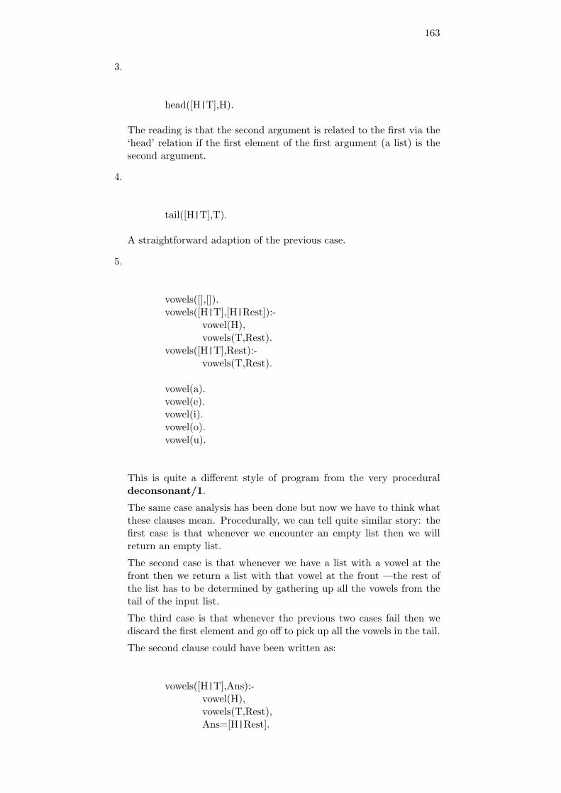
163
3.
head([H|T],H).
The reading is that the second argument is related to the first via the‘head’ relation if the first element of the first argument (a list) is thesecond argument.
4.
tail([H|T],T).
A straightforward adaption of the previous case.
5.
vowels([],[]).vowels([H|T],[H|Rest]):-
vowel(H),vowels(T,Rest).
vowels([H|T],Rest):-vowels(T,Rest).
vowel(a).vowel(e).vowel(i).vowel(o).vowel(u).
This is quite a different style of program from the very proceduraldeconsonant/1.
The same case analysis has been done but now we have to think whatthese clauses mean. Procedurally, we can tell quite similar story: thefirst case is that whenever we encounter an empty list then we willreturn an empty list.
The second case is that whenever we have a list with a vowel at thefront then we return a list with that vowel at the front —the rest ofthe list has to be determined by gathering up all the vowels from thetail of the input list.
The third case is that whenever the previous two cases fail then wediscard the first element and go off to pick up all the vowels in the tail.
The second clause could have been written as:
vowels([H|T],Ans):-vowel(H),vowels(T,Rest),Ans=[H|Rest].
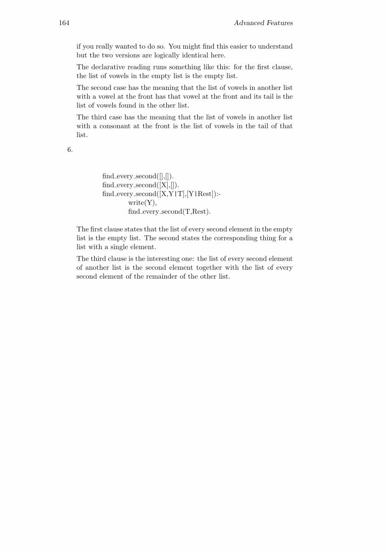
164 Advanced Features
if you really wanted to do so. You might find this easier to understandbut the two versions are logically identical here.
The declarative reading runs something like this: for the first clause,the list of vowels in the empty list is the empty list.
The second case has the meaning that the list of vowels in another listwith a vowel at the front has that vowel at the front and its tail is thelist of vowels found in the other list.
The third case has the meaning that the list of vowels in another listwith a consonant at the front is the list of vowels in the tail of thatlist.
6.
find every second([],[]).find every second([X],[]).find every second([X,Y|T],[Y|Rest]):-
write(Y),find every second(T,Rest).
The first clause states that the list of every second element in the emptylist is the empty list. The second states the corresponding thing for alist with a single element.
The third clause is the interesting one: the list of every second elementof another list is the second element together with the list of everysecond element of the remainder of the other list.

Appendix F
Solutions and Comments onExercises for Chapter ??
F.1 Exercise 6.1
All the programs in these examples can be done by selecting the right schemaand then instantiating it correctly.
1. We now produce solutions making use of the schema Test For Exis-tence.
list existence test(Info,[Head|Tail]):-element has property(Info,Head).
list existence test(Info,[Head|Tail]):-list existence test(Info,Tail).
(a) We discard all the parameters from the schema (Info). We re-name list existence test to an integer and element has propertyto integer. We will not show how the others programs are writ-ten using the schema.
an integer([H|T]):-integer(H).
an integer([H|T]):-an integer(T).
If the head of the list is an integer then the list contains an integer(this describes the first clause) —otherwise we require that thetail of the list has an integer somewhere (the second clause).
Note that the second clause does not strictly have to be sec-ond. The two clauses could be the other way round.
an integer([H|T]):-an integer(T).
an integer([H|T]):-integer(H).
165

166 Advanced Features
If this were so, however, the program would execute muchless efficiently. You could try defining the program both waysround and look at what happens using the trace command.What is going on? Either way round, we have the same declar-ative reading but the procedural reading is not so straightforward.For the first way, it goes roughly like this: examine the head ofthe list and stop with success if this is an integer —otherwisediscard the head of the list and examine the remainder forwhether it contains an integer. For the second way: throwaway the head of the list and examine the remainder to seewhether it has an integer in it —otherwise look at the headof the list to see whether it is an integer. This sounds verypeculiar but it works. What happens is that Prolog throwsaway all the elements, gets to the empty list and then fails.Backtracking now leads it to try showing that the list consist-ing of the last element in the original list is an integer: if thisis not so then further backtracking will lead Prolog to try thelist consisting of the last two elements of the original list hasan integer at the front of the list. This keeps on until eitheran integer is found (working back through the list) or there isno way to backtrack.
(b) has embedded lists([H|T]):-H=[Embeddedhead| Tail].
has embedded lists([H|T]):-has embedded lists(T).
A list has an element which is itself a (non-empty) list if the headof the list is a non-empty list (the first clause) or else the list’stail has an element in it that is a (non-empty) list (the secondclause).We can also rewrite this to perform implicit unification ratherthan the explicit unification H=[Embeddedhead| Tail]:
has embedded lists([[Embeddedhead| Tail]|T]).has embedded lists([H|T]):-
has embedded lists(T).
Does the order of these clauses matter? The same issues applyas with the previous example.
Note that if we want to fix the problem of extending the codeto handle the empty list as well we need:
has embedded lists([H|T]):-H=[].
has embedded lists([H|T]):-H=[Embeddedhead| Tail].
has embedded lists([H|T]):-has embedded lists(T).
That is, another clause to handle the case where the head ofthe list is an empty list.By the way, this can be rewritten as:
has embedded lists([[]|T]).has embedded lists([[Embeddedhead| Tail]|T]).has embedded lists([H|T]):-

167
has embedded lists(T).
That is, we can rewritethe explicit unification (H=[Embeddedhead| Tail] as animplicit unification.Why does this solution become dubious for e.g. the query?- has embedded lists([a,X,b])? The check that the headelement is a list will eventually encounter the equivalent ofX=[Embeddedhead| Tail] (or X=[]) —which will suc-ceed! Is this what is wanted? For then, a list containing avariable will always have an embedded list in it. This may beOK but we would want to know a little more before makinga decision.
2. We now produce solutions for the schema Test All Elements.
test all have property(Info,[]).test all have property(Info,[Head|Tail]):-
element has property(Info,Head),test all have property(Info,Tail).
(a) We discard all the parameters from the schema (Info).We rename test all have property to all integers and ele-ment has property to integer. We will not show how the othersprograms are written using this schema.
all integers([]).all integers([H|T]):-
integer(H),all integers(T).
We now require that every member of the input list has a commonproperty —viz that of being an integer.We note that the reading of the first clause is that every elementof the empty list is an integer. The second clause states that forevery list, every element is an integer if the head of the list is aninteger and every element of the remaining list is an integer.
(b) no consonants([]).no consonants([H|T]):-
vowel(H),no consonants(T).
vowel(a).vowel(e).vowel(i).vowel(o).vowel(u).
Again, the empty list is such that every element in it is not aconsonant. And, again, a list has no consonants if the head ofthe list (first element) is not a consonant and the remainder (tail)of the list has no consonants in it.

168 Advanced Features
We could have done this a little differently with the help of thepredicate \+/1.
no consonants([]).no consonants([H|T]):-
\+ consonant(H),no consonants(T).
consonant(b).consonant(c).(etc.)
The need to specify 26 consonants is a little tedious but accept-able.
3. We now produce the solutions that make use of the schema Return aResult —Having Processed One Element.
We use this schema:
return after event(Info,[H|T],Result):-property(Info,H),result(Info,H,T,Result).
return after event(Info,[Head|Tail],Ans):-return after event(Info,Tail,Ans).
(a) This one can be shown to be an example of the schema but the‘obvious’ solution doen’t fit exactly.
nth(1,[H|T],H).nth(N,[H|T],Ans):-
NewN is N-1,nth(NewN,T,Ans).
The first clause has the declarative reading that the first elementof the list is its head. The second clause has the declarativereading that the nth element of the list is the n-1th element ofthe list’s tail.It can be difficult to appreciate how this works. So the proceduralreading for the second clause can be taken as: to find the nthelement of the list, lop off the first element (the head) and thenlook for the n-1th element in the remainder of the list (the tail).Note that the order of the subgoals is important here. If anattempt is made to write this as:
nth(1,[H|T],H).nth(N,[H|T],Ans):-
nth(NewN,T,Ans),NewN is N-1.
then we get into trouble: when the first subgoal (assuming thefirst argument is an integer greater than 1) is executed then thevariable NewN will not be bound to an integer. This will meanthat once we have recursed down the list until the first clause suc-ceeds then we will have a number of subgoals awaiting execution

169
—the first of which will be 1 is Variable -1. This fails with anerror message as the is/2 predicate requires that the right handside (second argument) be an arithmetical expression and it isnot.
We can generate another solution with a little bit of trickery.nth2(N,[H|T],H):-
1 is N.nth2(N,[H|T],Ans):-
nth2(N-1,T,Ans).This, if you trace the execution, generates a series of subgoalsof the form nth2(somenumber-1-1-1-1-1...,list,variable. Thefirst clause succeeds when the first argument evaluates to 1.Note that the second clause is much neater as a consequence.The observant will notice that these various versions of nth/3do not fit the schema that well. This is partly because therecursion variable is the first argument and is on the naturalnumbers rather than lists.
(b) next(PossibleElement,[PossibleElement,NextElement|T],NextElement).next(PossibleElement,[H|T],Ans):-
next(PossibleElement,T,Ans).
This program has a straightforward (declarative) reading: thefirst clause states that the next element (third argument) afterthe named one (first argument) is when the list (second argument)begins with the named element and followed by the desired nextelement. Note the flexible use of the list notation which allowsthe user to specify a fixed number of elements at the front of alist (here, two).
(c)This solution fits the desired schema exactly (and also makes useof the schema Building Structure in the Clause Head).We use one parameter from the schema (Info). We rename re-turn after event to del 1st1, property to =, result to =. Thisresults in:
del 1st1(ToGo,[H|T],Ans):-H=ToGo,Ans=T.
del 1st1(ToGo,[H|T],[H|NewT]):-del 1st1(ToGo,T,NewT).
which can be rewritten to
del 1st1(ToGo,[ToGo|T],T).del 1st1(ToGo,[H|T],[H|NewT]):-
del 1st1(ToGo,T,NewT).
The declarative reading is that when the first argument is thehead of the list (which is the second argument) then the thirdargument is the tail (remainder) of the list —otherwise, the thirdargument is a list with the first element the same as that of thesecond argument and the tail is the list with the desired elementdeleted.

170 Advanced Features
We can also describe this procedurally, but we will assume thatit is intended that the third argument is output and the othertwo are inputs.When we find the desired element at the head of the input list(the second argument) then we return the tail of that list. Whenwe do not find this, we copy over the head into the output listand go looking for the result of deleting the desired element fromthe remainder (tail) of the input list.Now here is a ‘solution’ using the schema Building Structure inthe Clause Body.
del 1st2(ToGo,L,Ans):-del 1st2(ToGo,L,[],Ans).
del 1st2(ToGo,[ToGo|T],Acc,Ans):-append(Acc,T,Ans).
del 1st2(ToGo,[H|T],Acc,Ans):-del 1st2(ToGo,T,[H|Acc],Ans).
append([],L,L).append([H|L1],L2,[H|L3]):-
append(L1,L2,L3).
Note that we have defined a predicate del 1st2/3 which inter-faces to del 1st2/4 and initialises the accumulator (third argu-ment) to the empty list.The two clauses have a procedural reading: when we find thedesired element then we glue the accumulator onto the front ofthe remainder (tail) of the list found in the second argument usingappend/3 —otherwise, we copy the head of the list to the headof the accumulator and then try to delete the desired elementfrom the tail of the list using the new accumulator.
4. For each of these examples, we use the schema Return a Result —Having Processed All Elements. We have, however, two ways of writ-ing each with each way corresponding to a different (list processing)schema. These are, namely, Building Structure in the Clause Head andBuilding Structure in the Clause Body.
Here is the schema making use of the Building Structure in the ClauseHead:
process all(Info,[],[]).process all(Info,[H1|T1],[H2|T2]):-
process one(Info,H1,H2),process all(Info,T1,T2).
where process one/1 takes Info and H1 as input and outputs H2
(a) We keep one parameter from the schema (Info). We renameprocess all to nple1 and process one to is. We will not show howthe others programs are written using the schema.

171
nple1(N,[],[]).nple1(N,[H|T],[NewH|NewT]):-
NewH is N*H,nple1(N,T,NewT).
The declarative reading: every element in the empty list (third ar-gument) is the given multiple (first argument) of the correspond-ing element in the empty list (second argument) —otherwise, thelist found in the third argument position is in the desired relationto the list found in the second argument position if the head ofone list is the desired multiple of the head of the other list andthe desired relation holds between the tails of these two lists.
nple2(N,L,Ans):-nple2(N,L,[],Ans).
nple2(N,[],Ans,Ans).nple2(N,[H|T],Acc,Ans):-
NewN is N*H,nple2(N,T,[NewN|Acc],Ans).
Again, when using the schema Building Structure in the ClauseBody together with an accumulator, we define a predicatenple2/3 which initialises the accumulator for nple2/4.Now we have the procedural reading for nple2/4 assuming thatthe output list is the fourth argument, and the other argumentpositions are inputs.We return the result found in the accumulator once the inputlist is empty —otherwise we remove the head from the inputlist, multiply it by the desired amount, place the result in theaccumulator and repeat the process for the tail of the input listand the new accumulator.
(b)For this predicate, we need three cases to handle: the empty list,when the head of the list matches the element to be deleted andthe case where these two elements do not match.The first clause results from the observation that the empty listwith all the occurrences of the named element removed is theempty list.
del all1(ToGo,[],[]).del all1(ToGo,[ToGo|T],Ans):-
del all1(ToGo,T,Ans).del all1(ToGo,[H|T],[H|Ans]):-
del all1(ToGo,T,Ans).
The second clause is read declaratively as being true when theelement to be deleted unifies with the head of the list (secondargument) then the result of deleting all occurrences will be thesame as deleting all occurrences from the tail of that list.The third clause is the “otherwise” case: the result of deletingall occurrences from the list will is the head of the list together

172 Advanced Features
with the result of deleting all undesired occurrences from the tailof that list.
There is a serious problem here. If a program which makes useof del all1/3 backtracks to redo the call to del all1/3 thenwe will get some undesirable behaviour as this definition willgenerate false solutions (we assume here that we always calldel all1/3 with the second argument a list, the first argumentsome ground term (i.e. a term containing no variable) and thethird argument a variable).Consider the query del all1(a,[b,a,n,a,n,a],X). The first so-lution will result in X=[b,n,n]. Fine. But the last ‘a’was removed through a use of the second clause —the sub-goal would be del all1(a,[a],X 1) and originally producedX=[]. Now, on redoing, we try to satisfy the goal with thethird clause. The query del all1(a,[a],X 1) matches with thehead of the clause —del all1(ToGo,[H|T],[H|Ans])— re-sulting in ToGo=a, H=a, T=[] and X 1=[H|Ans] witha subgoal of del all1(a,[],Ans).. This gets satisfied withAns=[] and therefore we have another solution for the querydel all1(a,[a],X 1) —viz X 1=[a] and this is wrong.The problem arises because any query for which the secondargument is a non-empty list such that its head is the element-to-be-deleted will also be guaranteed to match the head of thethird clause. This means that there are ways of resatisfyingthe query which result in undesired (and wrong) solutions.How do we solve this? There are two basic ways —one ofwhich is fairly easy to read and the other relies on the use ofthe ‘cut’.
i. add an extra test condition to the third clause to ensurethat attempts to backtrack will fail. We make it impossi-ble for a goal to simultaneously match against the samegoal.
del all1(ToGo,[],[]).del all1(ToGo,[ToGo|T],Ans):-
del all1(ToGo,T,Ans).del all1(ToGo,[H|T],[H|Ans]):-
\+(H=ToGo),del all1(ToGo,T,Ans).
This is straightforward but does effectively require thatunification between the element-to-be-deleted and thehead of the list is done twice. Fine for simple checks butthis rapidly gets more expensive in more complex situa-tions. Now for the cut.
ii. a cut (!/0) can be placed to say that once clause 2 hasbeen used then never look for another match...this means:
del all1(ToGo,[],[]).del all1(ToGo,[ToGo|T],Ans):-
del all1(ToGo,T,Ans),!.del all1(ToGo,[H|T],[H|Ans]):-
del all1(ToGo,T,Ans).
This is much less easy to read but is generally more ef-ficient. Beginners, however, tend to spray cuts aroundproducing code like this:
del all1(ToGo,[],[]):-!.del all1(ToGo,[ToGo|T],Ans):-
del all1(ToGo,T,Ans),!.del all1(ToGo,[H|T],[H|Ans]):-

173
del all1(ToGo,T,Ans),!.
They do this because they do not understand the way thecut works. Because of this, the code written has effectsthey can’t predict or understand. Extra, useless cuts alsomeans a loss of efficiency. Therefore, we strongly recom-mend the first version.
Every program you write that is intended to succeed once andonce only should be checked to make sure that this will happenat the time you write the predicate.
The second version making use of the schema Building Structurein the Clause Body:
del all2(ToGo,L,Ans):-del all2(ToGo,L,[],Ans).
del all2(ToGo,[],Ans,Ans).del all2(ToGo,[ToGo|T],Acc,Ans):-
del all2(ToGo,T,Acc,Ans).del all2(ToGo,[H|T],Acc,Ans):-
del all2(ToGo,T,[H|Acc],Ans).
Again, we use del all2/3 to initialise the accumulator fordel all2/4.
Again, note that we would need protection against unexpectedbacktracking if this program is to be used in another program.Again, we would want a cut in the second clause of del all2/4.
(c)Here we have the version making use of the schema BuildingStructure in the Clause Head:
sum1([X],X).sum1([H|T],Ans):-
sum1(T,RestAns),Ans is RestAns+H.
In this first version, we have a straightforward declarative reading.The first clause reads that the sum of integers in a list with asingle (assumed) integer is that single integer. The second clausestates that the sum of integers in a list is found by summing theintegers in the tail of the list and then adding the head of the listto the result.Now for the version making use of an accumulator.
sum2(X,Y):-sum2(X,0,Y).
sum2([],Ans,Ans).sum2([H|T],Acc,Ans):-
NewAcc is Acc+H,sum2(T,NewAcc,Ans).
The second version uses an accumulator. Here, we make use ofsum2/2 to call sum3 with the accumulator initialised to 0. Inthis case, the first clause can br read procedurally as saying that

174 Advanced Features
once we have an empty list then the answer desired (third argu-ment) is the accumulated total (second argument). The secondclause states that we find the answer (third argument) by addingthe head of the list (first argument) to the accumulator (secondargument) and then repeating the process on the remainder ofthe list (with the accumulator set appropriately).

Appendix G
Solutions and Comments onExercises for Chapter ??
G.1 Exercise 8.1
1.
[the,clever,boy,buys,a,sweet][the,clever,sweet,buys,a,clever,clever,boy](etcetera)
These are legitimate inputs produced by the query
?- s([the,clever,boy,buys,a,sweet],[]).?- s([the,clever,sweet,buys,a,clever,clever,boy],[]).(etcetera)
It is not so immediately apparent that this grammar can generatesentences as well. What is the order in which sentences are generated?
[a,boy,buys,a,boy][a,boy,buys,a,sweet][a,boy,buys,the,boy][a,boy,buys,the,sweet][a,boy,buys,a,clever,boy][a,boy,buys,a,clever,sweet][a,boy,buys,a,clever,clever,boy][a,boy,buys,a,clever,clever,sweet][a,boy,buys,a,clever,clever,clever,boy](and so on)
2. Here is just one example —there are various ways of doing this.
s(sentence(NP-VP)) --> np(NP),vp(VP).
np(nounphrase(Det-N)) --> det(Det),noun(N).
175

176 Advanced Features
np(nounphrase(Det-Adjs-N)) --> det(Det),adjs(Adjs),noun(N).
vp(verbphrase(V-NP)) --> verb(V),np(NP).
det(determiner(a)) --> [a].det(determiner(the)) --> [the].adjs(adjectives(Adj)) --> adj(Adj).adjs(adjectives(Adj-Adjs)) --> adj(Adj),
adjs(Adjs).adj(adjective(clever)) --> [clever].noun(noun(boy)) --> [boy].noun(noun(sweet)) --> [sweet].verb(verb(buys)) --> [buys].
which produces (in a much less readable form than the following):
X = sentence(nounphrase(
determiner(a)-adjectives(adjective(clever))-noun(boy))
-verbphrase(
verb(buys)-nounphrase(
determiner(a)-adjectives(adjective(clever)-adjectives(adjective(clever)))-noun(boy))))
3. This is very hard to do in general. The issue here is one of ‘robustparsing’ and it is a major research topic. Consequently, there is nocomplete answer but a first attempt might look like:
s(sentence(NP-VP)) --> np(NP),vp(VP).
np(nounphrase(Det-N)) --> det(Det),noun(N).
np(nounphrase(Det-Adjs-N)) --> det(Det),adjs(Adjs),noun(N).
vp(verbphrase(V-NP)) --> verb(V),np(NP).
det(determiner(a)) --> [a].det(determiner(the)) --> [the].det(unknown det(X)) --> [X],

177
{\+(known(X))}.adjs(adjectives(Adj)) --> adj(Adj).adjs(adjectives(A-Adjs)) --> adj(A),
adjs(Adjs).adj(adjective(clever)) --> [clever].adj(unknown adj(X)) --> [X],
{\+(known(X))}.noun(noun(boy)) --> [boy].noun(noun(sweet)) --> [sweet].noun(unknown noun(X)) --> [X],
{\+(known(X))}.verb(verb(buys)) --> [buys].verb(unknown verb(X)) --> [X],
{\+(known(X))}.known(X):-noun(noun(X), , ).known(X):-verb(verb(X), , ).known(X):-det(determiner(X), , ).known(X):-adj(adjective(X), , ).
Some points to note:
(a) It cannot cope with missing words so this goal fails badly. Wecould try to extend it to meet this problem. For example, wemight like the following query to succeed:
s(X,[the,clever,buys,a,sweet],[]).
(b) It does cope quite well with more than one misspelling providedthe sentence structure is acceptable —as in the query:
s(X,[the,clever,silly,buoy,buys,a,sweet],[]).
(c) The known/1 predicate is not at all clever.

Appendix H
Solutions and Comments onExercises for Chapter ??
H.1 Exercise 9.1
1. First, we examine the execution of the query female author. Wetake the first clause for female author/0 and solve for author(X).We use the first clause of author/1 and solve the resulting subgoal,name(X), using the first clause of name/1 to get X=sartre. Thesubgoals write(X), write(’ is an author’) and nl succeed with theside-effect of writing:
sartre is an author
on the screen. Then we solve the subgoal female(X) with X stillbound to sartre. Neither of the heads of the clauses for female/1match the goal female(sartre) so Prolog fails and backtracks. Wekeep backtracking until we get to redo the subgoal author(X). Thismeans that we now try to redo name(X) and we satisfy this withX=calvino. Again, we generate the side-effect on the screen of
calvino is an author
and try to satisfy female(X) with X bound to calvino. Again, thisfails and we backtrack. Again, the subgoal name(X) can be satisfied—this time, for the last time, with X=joyce. On the screen we get
joyce is an author
and another attempt to prove that female(X) with X=joyce (whichfails). This time, on backtracking, there are no more solutions forname(X). We now move on to resatisfy author(X) by using its sec-ond clause. This generates, on the screen,
no more found!
then fails. We now backtrack and, since there are no more ways ofsatisfying author(X), we are through with the first clause of fe-male author/0. The second succeeds by writing
178

179
no luck!
and succeeds.
We now explain how to place the cuts to get the desired outputs.
(a) The first solution requires the use of one cut to produce the side-effect:
sartre is an authorno more found!no luck!
Note that, compared with before, we have much the same but weinfer that there is only one solution for name(X). This suggeststhat we place the cut so that name(X) succeeds once only. Thiscan be done by rewriting the first clause of name/1 as
name(sartre):-!.
(b) The next solution requires the use of one cut to produce the side-effect:
sartre is an authorcalvino is an authorjoyce is an authorno more found!
Compared with the original output, we observe that the phrase‘no luck!’ is not generated. This suggests that we want to commitourselves to the first clause of female author and not use thesecond at all. Hence we have the solution:
female author:- !,author(X),write(X),and so on
but note that now the original query fails after producing thedesired side-effect.Also note that we have to put the cut before the call to author/1—otherwise we would only generate one of the names rather thanall three.
(c) The next solution requires the use of one cut to produce the side-effect:
sartre is an authorno luck!
This time we observe that we only get one name and we don’tgenerate the phrase ‘no more found!’. This suggest that we wantauthor(X) to succeed once and once only —and go on to use thesecond clause of female author (this suggests that the cut can-not be one of the subgoals in the first clause of female author).We don’t want to generate the phrase ‘no more found’ —so thissuggests that we commit to the first clause of author/1. We willput a cut in the body of this clause —but where? If we put itthus:
author(X):- !,name(X).

180 Advanced Features
then we would generate all three names by backtracking. Hencethe desired solution is:
author(X):- name(X),!.
We can read this as being committed to the first, and only thefirst, solution for name(X).
(d) The next solution requires the use of one cut to produce the side-effect:
sartre is an author
Now we don’t want to generate either ‘no more found!’ or ‘noluck!’ —and we only want one of the names generated.So we definitely want to be committed to the first clause of fe-male author/0. This suggests putting the cut in the body ofthe first clause of this predicate —but where? If we put it afterthe subgoal female(X) then we would get all three solutions toname(X) and their associated side-effects. If we put it beforeauthor(X) we also get roughly the same. Therefore we wantsomething like:
female author:- author(X),!,write(X),and so on
(e) The next solution requires the use of one cut to produce the side-effect:
sartre is an authorcalvino is an authorjoyce is an authorno luck!
Now we don’t get the message ‘no more found!’. This suggeststhat we want to commit to the first clause of author/1. If we putthe cut after the subgoal name(X) then we will commit to thefirst solution and not be able to generate the other two. Hencewe must put the cut before as in:
author(X):- !,name(X).
2. We will assume a mode of mode delete(+,+,?). i.e. the first twoarguments are always completely instantiated and the third argumentcan be either instantiated or a variable.
delete([], , []).delete([Kill|Tail], Kill, Rest) :-
delete(Tail, Kill, Rest),!.delete([Head|Tail], Kill, [Head|Rest]):-
delete(Tail, Kill, Rest).
The cut is placed in the body of the second clause. This is needed be-cause, in the code given in the probem, any usage of the second clauseto delete an element allows the query to be resatisfied on redoing.This is caused by the fact that any query matching the head of thesecond clause will also match the head of the third clause.

181
3. To define disjoint/2, here is the solution found in the standard DEC-10 library.
% disjoint(+Set1, +Set2)% is true when the two given sets have no elements in common.% It is the opposite of intersect/2.
disjoint(Set1, Set2) :-member(Element, Set1),memberchk(Element, Set2),!, fail.
disjoint( , ).
member(X,[X|Rest]).member(X,[Y|Rest]):-
member(X,Rest).
memberchk(X,[X|Rest]):- !.memberchk(X,[Y|Rest]):-
memberchk(X,Rest).
Note the definition is quite interesting: First, note that we make use ofthe generate—test schema: the first clause of disjoint/2 uses mem-ber/2 as a (finite) generator to generate each of the elements in thefirst list one by one. Next, the solution is tested using memberchk/2for the second set. Second, if the element is in both sets then we meetthe cut—fail schema. This means the call to disjoint/2 fails. If thegenerated element never passes the test, then the attempt tosatisfy thecall to disjoint/2 using the first clause fails and we use the secondclause which makes use of a catch-all condition.
Other solutions are possible:
disjoint(Set1, Set2) :-\+(member(Element, Set1), member(Element, Set2)).
Here, disjoint succeeds whenever it is impossible to find a commonelement for both lists. If such an element exists then it fails.
4. To define plus/3:
plus(A, B, S) :-integer(A),integer(B),!,S is A+B.
plus(A, B, S) :-integer(A),integer(S),!,B is S-A.
plus(A, B, S) :-

182 Advanced Features
integer(B),integer(S),!,A is S-B. plus(A, B, S) :-plus error message(A, B, C).
The first three clauses cope with the cases where two or more of thearguments to plus/3 are instantiated to integers.
We need the cut to implement a commit schema as we don’t havedisjoint cases.
The last clause is intended to point out to the programmer that aninstantiation fault has occurred. The exact form of the message is upto you.

Appendix I
Solutions and Comments onExercises for Chapter ??
I.1 Exercise 11.1
1. Here is the answer in Prolog Form:
:(rule31,if(then(and(=(of(colour,wine),white),
and(or(=(of(body,wine),light), =(of(body,wine),medium)),or(=(of(sweetness,wine),sweet),=(of(sweetness,wine),medium)))),
then confidence factor(=(wine,riesling),1000))))
The tree is up to you!
183

Appendix J
Solutions and Comments onExercises for Chapter ??
J.1 Exercise 12.1
1. We want the following behaviour:
?- diff append([a,b|X]-X,[c,d,e|Y]-Y,Answer).Answer = [a,b,c,d,e|Y] - Y
Here is the solution:
diff append(List1-Tail1,Tail1-Tail2,List1-Tail2).
2. We want the following behaviour:
?- add at end(e,[a,b,c,d|X]-X,Answer).Answer = [a,b,c,d,e|Y] - Y
Here is the solution:
add at end(X,List-Tail,List-NewTail):-Tail=[X|NewTail],!.
add at end(X,List-[X|NewTail],List-NewTail).
Note the need to add the cut (!/0) to prevent unwanted behaviour onbacktracking to redo a call to this predicate.
3. We want the following behaviour:
?- diff reverse([a,b,c|X]-X,Answer).Answer = [c,b,a|Y] - Y
184

185
There are two cases: the first covers the case where we have the dif-ference list equivalent of the empty list.
The second case covers every other situation: we have to take off thehead element, reverse the remaining difference list and then stick theelement at the end of the difference list. We use add at end/3 thatwe have already defined.
Here is a solution:
diff reverse(X-X,Y-Y):-var(X),!.
diff reverse([H|List]-Tail,Answer):-diff reverse(List-Tail,NewDiffList),add at end(H,NewDiffList,Answer).
Note that, for the first clause, we state that the tail of the input isa variable (via var/1). The use of cut (!/0) is necessary to stopunwanted behaviour if we ever backtrack to redo this goal.
Also note that we will get nasty behaviour if the predicateadd at end/3 has not been defined to prevent unwanted behaviouron backtracking.
4. We want the following behaviour —assuming that the list is composedof integers or atoms or lists of these. This means that every element iseither the empty list, a list or some Prolog term that is atomic. i.e.the term satisfies atomic/1.
?- diff flatten([1,2,[3,4,[5,4,[3],2],1],7|X]-X,Ans).Ans=[1,2,3,4,5,4,3,2,1,7|Z]-Z
We have three cases: we are going to flatten the empty list by out-putting the difference list version of [] —i.e. X-X. We flatten an‘atomic’ element other than the empty list by returning a differencelist with a single element —viz [someelement|X]-X. The third caseis designed to handle the case where the head of the first argument isa list. In this case, we flatten the head, and then flatten the tail.
Here is a solution:
diff flatten([H|T],X-Y):-diff flatten(H,X-Z),diff flatten(T,Z-Y).
diff flatten(X,[X|T]-T):-atomic(X),\+(X=[]).
diff flatten([],X-X).
Note how the result of flattening the head is a difference list with a hole.We get the same for flattening the tail and join the lists together byidentifying the hole for the flattened head with the open list resultingfrom flattening the tail.

186 Advanced Features
5. We want the following behaviour:
?- diff quicksort([3,1,2|X]-X,Ans).Ans=[1,2,3|Z]-Z
We should note that the obvious advantage in using difference listshere is in avoiding the various calls to append/3 which can get veryexpensive. On the other hand, we have to realise that there is anoverhead in carrying difference lists around in this form.
Here is a solution:
diff quicksort(X-X,Y-Y):-var(X).
diff quicksort([H|T]-Hole1,Ans-Hole2):-diff split(H,T-Hole1,SmallDiffList,BigDiffList),diff quicksort(SmallDiffList,Ans-[H|Z]),diff quicksort(BigDiffList,Z-Hole2).
diff split( ,X-X,Y-Y,Z-Z):-var(X).
diff split(X,[Y|Tail]-Hole1,[Y|Small]-Hole2,BigDiffList):-X > Y,diff split(X,Tail-Hole1,Small-Hole2,BigDiffList).
diff split(X,[Y|Tail],SmallDiffList,[Y|Big]-Hole2):-X =< Y,diff split(X,Tail,SmallDiffList,Big-Hole2).
The correspondence between the difference and proper list versions isclose.
Wherever we have an empty list ([]) we introduce the differencelist version (X-X). We have to be careful to distinguish unrelatedempty lists. For example, consider the first clause of quicksort/2in the notes: quicksort([],[]). The correspondence might suggestdiff quicksort(X-X,X-X). But in this case, there can be very un-pleasant consequences as we are forcing certain variables to be identi-cal that might have been distinct up to the point of solving the goaldiff quicksort(A,B). Consequently, we introduce different version ofthe difference list ‘empty list’ and write diff quicksort(X-X,Y,Y).
Note that the ‘stopping condition’ is that we have run out of elementsto sort by reaching the ‘hole’. This means the test is for having en-countered a variable. So the procedural reading of the first clause iseffectively: return a difference list equivalent to the ‘empty list’ whenwe find that we have consumed all the non-variable elements from thefront of the list. To do this, we use var/1 which takes a Prolog termas input and is true whenever that term is an uninstantiated variable(it can be bound to another uninstantiated variable though).
The remaining two clauses are structurally very similar to the last twoclauses for quicksort/2 as in the notes. The main difference is theloss of the call to append/3 and the means by which we can partially

187
‘fill in’ the hole of the Small difference list with the result of sortingthe Big difference list.
As for, diff split/4, we have a very similar situation which we notexplain further here.
What about the efficiency? Is diff quicksort/2 faster than quick-sort/2? And are we comparing like with like? The empirical answer isthat quicksort/2 is faster (there are ways of improving the efficiencyof the above version of diff quicksort/2 but they are not sufficient)!
One reason why this version of diff quicksort/2 is slower than quick-sort/2 is that the former predicate transforms a difference list into adifference list while the latter transforms a proper list to a proper list.An improvement is achieved by writing a version that takes a properlist to a difference list as with:
diff quicksort v2([],[]).diff quicksort v2([H|T],Ans-Hole2):-
split(H,T,SmallProperList,BigProperList),diff quicksort v2(SmallProperList,Ans-[H|Z]),diff quicksort v2(BigProperList,Z-Hole2).
Note that we can now use the same split/4 as for quicksort/2.
The efficiency of this version is now better than the performance ofquicksort/2.
6. This one is up to you!