Embed Size (px)
Citation preview
Profile-based Virtual Machine Placement for EnergyOptimization of Data Centres
A THESIS SUBMITTED TO
THE SCIENCE AND ENGINEERING FACULTY
OF QUEENSLAND UNIVERSITY OF TECHNOLOGY
IN FULFILMENT OF THE REQUIREMENTS FOR THE DEGREE OF
MASTER BY RESEARCH
Zhe Ding
School of Electrical Engineering and Computer Science
Science and Engineering Faculty
Queensland University of Technology
2017


Copyright in Relation to This Thesis
c© Copyright 2016 by Zhe Ding. All rights reserved.
Statement of Original Authorship
The work contained in this thesis has not been previously submitted to meet requirements for an
award at this or any other higher education institution. To the best of my knowledge and belief,
the thesis contains no material previously published or written by another person except where
due reference is made.
Signature
Date:
i
QUT Verified Signature

ii

To my motherland
iii

iv
Abstract
The demand of cloud computing, in both scale and reliability, sustains a skyrocketing trend in
recent years. As the core infrastructure of cloud computing, more and more virtualized data
centers are being built worldwide. However, the huge amount of power consumption in data
centers, especially from servers, is a frustrating problem. This thesis addresses this problem
through profile-based virtual machine placement for improved energy efficiency. It formulates
the problem as a profile-based optimization problem. Then, it designs a profile-based virtual
machine placement framework to solve the optimization problem. The framework consists of
the three following phases:
1. Profiling: to analyze and build energy-aware profiles of tasks and jobs from data center
logs for profile-based virtual machine placement;
2. Task Classification: to classify tasks into three categories C permanent, normal-size and
tiny tasks for energy-efficient virtual machine placement; and
3. Virtual Machine Placement: from the outcomes of the previous two phases, to place
virtual machines to physical machines with enhanced energy efficiency.
These three phases are claimed as the major contributions of the thesis. Experiments are
conducted to verify the feasibility and energy efficiency of the presented framework. More
energy savings have been achieved from the framework over the widely used original First Fit
Decrease algorithm for all experiments of small-, medium-, and large-scale data centers.
v

vi
Keywords
data center, energy optimization, virtual machine placement, profiles, task classification
vii

viii
Acknowledgments
Most thanks to Professor Yu-chu Tian for making greatest effort towards the fulfilment of this
thesis, as well as supervising all relevant research stages, including formulation, design, and
experiments. Thanks, again, to this kind and hard-working professor.
Great thanks to my parents. They brought me into this wonderful world, gave me rigoros
educationand talent , and now are still supporting me doing research work here. This thesis
represents all the effort they have made during these decades.
Thanks to my motherland. The culture and tradition in that land taught me to be inclusive,
to have perseverance, and to be passionate. I shall never forget the air, aqua, and taste of this
land.
Finally, thank you my friends. Thank you anyone around me, or thousands of miles away,
in another corner in this world. Thank you, everyone in this world. Thank you, world.
ix

x
Table of Contents
Abstract v
Keywords vii
Acknowledgments ix
Nomenclature xv
List of Figures xviii
List of Tables xix
1 Introduction 1
1.1 Overview . . . . . . . . . . . . . . . . . . . . . . . . . . . . . . . . . . . . . 1
1.2 Problem Statement . . . . . . . . . . . . . . . . . . . . . . . . . . . . . . . . 3
1.2.1 Operating Cost of Data Centers . . . . . . . . . . . . . . . . . . . . . 3
1.2.2 Power Delivery Challenge . . . . . . . . . . . . . . . . . . . . . . . . 4
1.2.3 Cooling and Fireproofing Trouble . . . . . . . . . . . . . . . . . . . . 4
1.2.4 Negative Environment Impacts . . . . . . . . . . . . . . . . . . . . . . 5
1.3 Technical Gaps . . . . . . . . . . . . . . . . . . . . . . . . . . . . . . . . . . 6
1.3.1 Technical Gaps . . . . . . . . . . . . . . . . . . . . . . . . . . . . . . 6
1.3.2 Feasibility of this Topic . . . . . . . . . . . . . . . . . . . . . . . . . 7
1.4 Research Objectives and Contributions . . . . . . . . . . . . . . . . . . . . . . 7
1.4.1 Research Objectives . . . . . . . . . . . . . . . . . . . . . . . . . . . 7
xi
1.4.2 Research Contributions . . . . . . . . . . . . . . . . . . . . . . . . . . 8
1.5 Thesis Organization . . . . . . . . . . . . . . . . . . . . . . . . . . . . . . . . 9
2 Literature Review 11
2.1 Virtualization Technology . . . . . . . . . . . . . . . . . . . . . . . . . . . . 11
2.2 Virtual Machine . . . . . . . . . . . . . . . . . . . . . . . . . . . . . . . . . . 12
2.2.1 Hosted VMs . . . . . . . . . . . . . . . . . . . . . . . . . . . . . . . 13
2.2.2 Application-level VMs . . . . . . . . . . . . . . . . . . . . . . . . . . 14
2.2.3 Hypervisor VMs . . . . . . . . . . . . . . . . . . . . . . . . . . . . . 14
2.3 VM Management . . . . . . . . . . . . . . . . . . . . . . . . . . . . . . . . . 15
2.3.1 OnCOff Switching . . . . . . . . . . . . . . . . . . . . . . . . . . . . 16
2.3.2 Computing Resource Allocation . . . . . . . . . . . . . . . . . . . . . 16
2.3.3 VM Migration . . . . . . . . . . . . . . . . . . . . . . . . . . . . . . 17
2.4 Green Cloud Architecture . . . . . . . . . . . . . . . . . . . . . . . . . . . . . 18
2.5 VM Scheduling Strategies . . . . . . . . . . . . . . . . . . . . . . . . . . . . 19
2.6 Specific VM Scheduling Schemes . . . . . . . . . . . . . . . . . . . . . . . . 21
2.7 Recent Commercial Implementation . . . . . . . . . . . . . . . . . . . . . . . 22
2.7.1 Xen . . . . . . . . . . . . . . . . . . . . . . . . . . . . . . . . . . . . 22
2.7.2 VMware . . . . . . . . . . . . . . . . . . . . . . . . . . . . . . . . . 23
2.8 Profiles . . . . . . . . . . . . . . . . . . . . . . . . . . . . . . . . . . . . . . 23
2.9 Summary of Literature Review . . . . . . . . . . . . . . . . . . . . . . . . . . 25
3 Formulation and Design 27
3.1 Energy Consumption Model . . . . . . . . . . . . . . . . . . . . . . . . . . . 27
3.1.1 CPU Power . . . . . . . . . . . . . . . . . . . . . . . . . . . . . . . . 28
3.1.2 CPU Runtime . . . . . . . . . . . . . . . . . . . . . . . . . . . . . . . 29
3.1.3 Data Center Power Model . . . . . . . . . . . . . . . . . . . . . . . . 30
3.2 VM Placement Model . . . . . . . . . . . . . . . . . . . . . . . . . . . . . . . 30
xii
3.3 Energy Optimization Objective . . . . . . . . . . . . . . . . . . . . . . . . . . 31
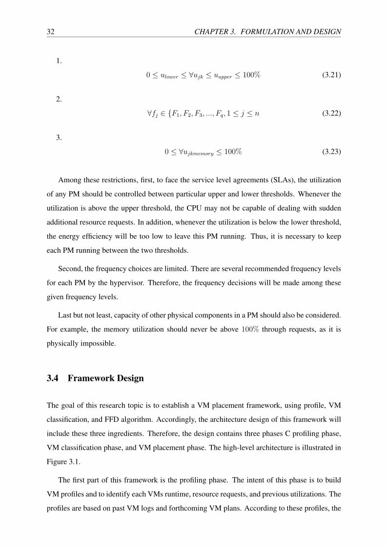
3.4 Framework Design . . . . . . . . . . . . . . . . . . . . . . . . . . . . . . . . 32
3.5 Experimental Design . . . . . . . . . . . . . . . . . . . . . . . . . . . . . . . 33
3.6 Chapter Summary . . . . . . . . . . . . . . . . . . . . . . . . . . . . . . . . . 36
4 Profiling and Profile Building 37
4.1 VM Profile . . . . . . . . . . . . . . . . . . . . . . . . . . . . . . . . . . . . 37
4.2 Profiling . . . . . . . . . . . . . . . . . . . . . . . . . . . . . . . . . . . . . . 38
4.3 Building Profiles . . . . . . . . . . . . . . . . . . . . . . . . . . . . . . . . . 39
4.4 Large-scale Experiments . . . . . . . . . . . . . . . . . . . . . . . . . . . . . 41
4.5 Medium-scale Experiments . . . . . . . . . . . . . . . . . . . . . . . . . . . . 45
4.6 Small-scale Experiments . . . . . . . . . . . . . . . . . . . . . . . . . . . . . 45
4.7 Chapter Summary . . . . . . . . . . . . . . . . . . . . . . . . . . . . . . . . . 46
5 Task Classification 49
5.1 Task Characteristics . . . . . . . . . . . . . . . . . . . . . . . . . . . . . . . . 49
5.2 Deisgn of Task Classes . . . . . . . . . . . . . . . . . . . . . . . . . . . . . . 50
5.3 Task Separation and Assignment Design . . . . . . . . . . . . . . . . . . . . . 52
5.3.1 Job and Task Separation . . . . . . . . . . . . . . . . . . . . . . . . . 53
5.3.2 Assignment of Tasks into VMs . . . . . . . . . . . . . . . . . . . . . . 54
5.4 Related Experiments . . . . . . . . . . . . . . . . . . . . . . . . . . . . . . . 55
5.4.1 Large-scale Experiments . . . . . . . . . . . . . . . . . . . . . . . . . 55
5.4.2 Medium-scale Experiments . . . . . . . . . . . . . . . . . . . . . . . 56
5.4.3 Small-scale Experiments . . . . . . . . . . . . . . . . . . . . . . . . . 58
5.4.4 Discussions on Experiments . . . . . . . . . . . . . . . . . . . . . . . 60
5.5 Chapter Summary . . . . . . . . . . . . . . . . . . . . . . . . . . . . . . . . . 60
6 Profile-based Virtual Machine Placement 63
6.1 Profile-based VM Placement Scheme . . . . . . . . . . . . . . . . . . . . . . 63
xiii

6.2 Profile-based VM Placement Architecture . . . . . . . . . . . . . . . . . . . . 65
6.3 FFD Algorithm in Profile-based VM Placement . . . . . . . . . . . . . . . . . 65
6.4 Large-scale Experiments . . . . . . . . . . . . . . . . . . . . . . . . . . . . . 66
6.4.1 Experiment Description . . . . . . . . . . . . . . . . . . . . . . . . . 67
6.4.2 Experiment Results . . . . . . . . . . . . . . . . . . . . . . . . . . . . 69
6.5 Medium-scale Experiments . . . . . . . . . . . . . . . . . . . . . . . . . . . . 71
6.5.1 Experiment Description . . . . . . . . . . . . . . . . . . . . . . . . . 71
6.5.2 Experiment Results . . . . . . . . . . . . . . . . . . . . . . . . . . . . 72
6.6 Small-scale Experiments . . . . . . . . . . . . . . . . . . . . . . . . . . . . . 74
6.6.1 Experiment Description . . . . . . . . . . . . . . . . . . . . . . . . . 74
6.6.2 Experiment Results . . . . . . . . . . . . . . . . . . . . . . . . . . . . 75
6.7 Evaluation . . . . . . . . . . . . . . . . . . . . . . . . . . . . . . . . . . . . . 76
6.7.1 Energy Evaluation . . . . . . . . . . . . . . . . . . . . . . . . . . . . 76
6.7.2 Execution Time and Scalability Analysis . . . . . . . . . . . . . . . . 78
6.8 Chapter Summary . . . . . . . . . . . . . . . . . . . . . . . . . . . . . . . . . 79
7 Conclusions and Recommendations 81
7.1 Summary of the Research . . . . . . . . . . . . . . . . . . . . . . . . . . . . . 81
7.2 Recommendations and Future Work . . . . . . . . . . . . . . . . . . . . . . . 82
Literature Cited 86
xiv
Nomenclature
Abbreviations
BFD best fit decrease (algorithm)
CPU Central Processing Unit
C-state CPU sleeping state
DPM Distributed Power Management
DRS Distributed Resource Scheduler
DVFS dynamic voltage and frequency scaling
FFD first fit decrease (algorithm)
GA genetic algorithm
IaaS infrastructure as a service
PM physical machine
P-state power-performance state
PSU power supply unit
QoS quality of service
ROI return on investment
SLA service level agreement
VM virtual machine
VMM virtual machine monitors
VNC virtual network computing
Symbols
xv
E energy
P power
t time
V voltage
f frequency
a CPU architecture constant
C CPU capacity
γ power of voltage to frequency
b The coefficient for the correlation between voltage and frequency
op The option for a virtual machine
p The placement decision of a virtual machine
m The migration decision of a virtual machine
vm A virtual machine
r The resource request of a virtual machine
xvi
List of Figures
1.1 CPU power model. . . . . . . . . . . . . . . . . . . . . . . . . . . . . . . . . 7
2.1 VM state transitions for jobs and tasks. . . . . . . . . . . . . . . . . . . . . . . 24
3.1 VM Placement Framework Architecture . . . . . . . . . . . . . . . . . . . . . 33
3.2 Experiment Design . . . . . . . . . . . . . . . . . . . . . . . . . . . . . . . . 34
4.1 Segment of VM profile sample. . . . . . . . . . . . . . . . . . . . . . . . . . . 42
4.2 Entire peak CPU usage in 24 hours. . . . . . . . . . . . . . . . . . . . . . . . 42
4.3 Total CPU request and mean CPU usage in large-scale data centre. . . . . . . . 43
4.4 Total CPU request and peak CPU usage in large-scale data centre. . . . . . . . 44
4.5 Timely number of jobs in large-scale data centre. . . . . . . . . . . . . . . . . 44
4.6 Total CPU request in medium-scale data centre. . . . . . . . . . . . . . . . . . 45
4.7 Total job number in medium-scale data centre. . . . . . . . . . . . . . . . . . . 46
4.8 Total CPU request in small-scale data centre. . . . . . . . . . . . . . . . . . . 47
4.9 Total job number in small-scale data centre. . . . . . . . . . . . . . . . . . . . 47
5.1 Classification target. . . . . . . . . . . . . . . . . . . . . . . . . . . . . . . . 51
5.2 Separation & assignment flowchart. . . . . . . . . . . . . . . . . . . . . . . . 53
5.3 Large-scale classification result for permanent jobs. . . . . . . . . . . . . . . . 56
5.4 Number of tiny tasks in the large-scale data center. . . . . . . . . . . . . . . . 57
5.5 Number of VMs from tiny tasks in the large-scale data center. . . . . . . . . . 57
5.6 Medium-scale classification result for permanent jobs. . . . . . . . . . . . . . 58
xvii

5.7 Number of tiny tasks in the medium-scale data center. . . . . . . . . . . . . . . 58
5.8 Number of VMs from tiny tasks in the medium-scale data center. . . . . . . . . 59
5.9 Small-scale classification result for permanent jobs. . . . . . . . . . . . . . . . 59
5.10 Number of tiny tasks in the small-scale data center. . . . . . . . . . . . . . . . 60
5.11 Number of VMs from tiny tasks in the small-scale data center. . . . . . . . . . 61
6.1 Profile-based VM placement architecture. . . . . . . . . . . . . . . . . . . . . 66
6.2 FFD algorithm design. . . . . . . . . . . . . . . . . . . . . . . . . . . . . . . 67
6.3 VM placement experimental design. . . . . . . . . . . . . . . . . . . . . . . . 69
6.4 Large-scale VM placement experimental result: timely PM quantity. . . . . . . 70
6.5 Large-scale VM placement experiment result: PM number overlap. . . . . . . . 71
6.6 Large-scale VM placement experiment result: average PM utilization. . . . . . 72
6.7 Medium-scale VM placement experiment result: timely PM quantity. . . . . . . 73
6.8 Medium-scale VM placement experiment result: PM quantity overlap. . . . . . 73
6.9 Medium-scale VM placement experiment result: average PM utilization . . . . 74
6.10 Small-scale VM placement experiment result: timely PM quantity. . . . . . . . 75
6.11 Small-scale VM placement experiment result: PM quantity overlap. . . . . . . 76
6.12 Small-scale VM placement experiment result: average PM utilization. . . . . . 77
6.13 Execution time. . . . . . . . . . . . . . . . . . . . . . . . . . . . . . . . . . . 78
xviii
List of Tables
3.1 PM capacity and configuration . . . . . . . . . . . . . . . . . . . . . . . . . . 35
3.2 Number of PMs. . . . . . . . . . . . . . . . . . . . . . . . . . . . . . . . . . . 35
3.3 VM configuration in normalized CPU capacity. . . . . . . . . . . . . . . . . . 36
4.1 VM profile design. . . . . . . . . . . . . . . . . . . . . . . . . . . . . . . . . 40
4.2 Job profile design. . . . . . . . . . . . . . . . . . . . . . . . . . . . . . . . . . 40
6.1 Total energy evaluation. . . . . . . . . . . . . . . . . . . . . . . . . . . . . . . 77
xix

xx

Chapter 1
Introduction
In order to help solve the problem of huge energy consumption in data centers, this thesis
delivers a new virtual machine (VM) placement framework, including profiles and task clas-
sification. This framework aims to save power through profile-based resource allocation in
all three levels C application level, virtualization level, and physical level C in virtualized
data centers. Consequently, according to simulation results, this new framework has achieved
performance enhancements in the contributions of cloud infrastructure energy optimization,
sustainable national resource strategies, and carbon-dioxide emission limitation.
1.1 Overview
Designers and developers in the field of computing systems are already focused on the im-
provement of performance. Based on this particular foundational objective, the performance of
computing systems has been growing rapidly, along with, by Moores law, efficient design and
the growing density of the components [Moore, 2006].
However, even though the power efficiency calculated by performance per watt ratio has
gained a significant increase, the entire energy consumption of computing systems is rarely
decreasing [Beloglazov et al., 2011]. In addition, the power consumption amount has increased
by about 115 percent in only five years, from 70.8TWh in 2000 to 152.5TWh in 2005, which
might stand for 0.97 percent of the overall energy spent worldwide in 2005 [Mobius et al.,
2014].
Unfortunately, however, this huge power consumption has not been abundantly noticed by
1

2 CHAPTER 1. INTRODUCTION
system administrators through management methods. For example, server utilization, which
could be strictly related to the power usage ratio, is often neglected by many administrators. As
reported by Network World, over 75 percent of data center managers could only have a brief
view of the current dynamic usage of servers, and about 10 percent to 30 percent of their servers
may be doing nothing while being left on. With the lack of power-aware server management,
more electricity could outflow continuously without any production output. As a result, some
feasible measures need to be taken urgently to improve the energy efficiency in this server-
management field.
Data centers have already started to explore improvements in flexibility and usability by
virtualization technology. Many computing service providers, such as Google, Microsoft, Ama-
zon, and IBM, are rapidly implementing their data centers into highly virtualized environments,
and provide cloud services through this virtualized platform, without adequate awareness of the
power usage ratio as well [Beloglazov et al., 2011]. However, in the same article by Buyya
[Buyya et al., 2010], the new Green Cloud computing thinking might not meet the requirements
of this recent situation, as it is envisioned to achieve not only high computing performance but
also minimized power consumption. Thus, it would be necessary to gain some VM management
based on power-aware thinking. One of the effective measures of this is VM scheduling for
energy optimization [Monteiro et al., 2014].
As estimated, since the beginning of this century, the power consumption of data centers
has been skyrocketing continuously, which is also claimed by Network World. Unfortunately,
this issue has raised some far-reaching problems, such as huge operating costs in data centers,
bottlenecks of VM performance through power delivery challenges, cooling and fireproofing
difficulties, and negative environmental impacts of significant carbon dioxide emission and
natural resource consumption [Beloglazov et al., 2011]. However, this problem is not only
related to the infrastructure itself, but also strongly to deployed infrastructure management
methods. Thus, companies like Google, Microsoft, and Amazon have been implementing
new energy-aware data center management methods to achieve a higher return on investment
(ROI), quality of service (QoS), and service level agreements (SLAs) [Buyya et al., 2010].
In accordance with the urgency of this issue, this research topic also examines possible VM
management methods for energy optimization to help relieve these problems.
1.2. PROBLEM STATEMENT 3
1.2 Problem Statement
Currently, information and communication technology could occupy as much as nearly 3 per-
cent of the entire global electricity consumption, and almost half of this is consumed by data
service-like servers and data centers [Zhou and Jiang, 2014]. However, the frustrating issue is
not only in the amount of energy consumed, but also its increasing rate of growth. As mentioned
above, worldwide data center power consumption percentage rose from 0.53 percent in 2000 to
0.97 percent in 2005, and even probably to 1.50 percent in 2010 [Mobius et al., 2014].
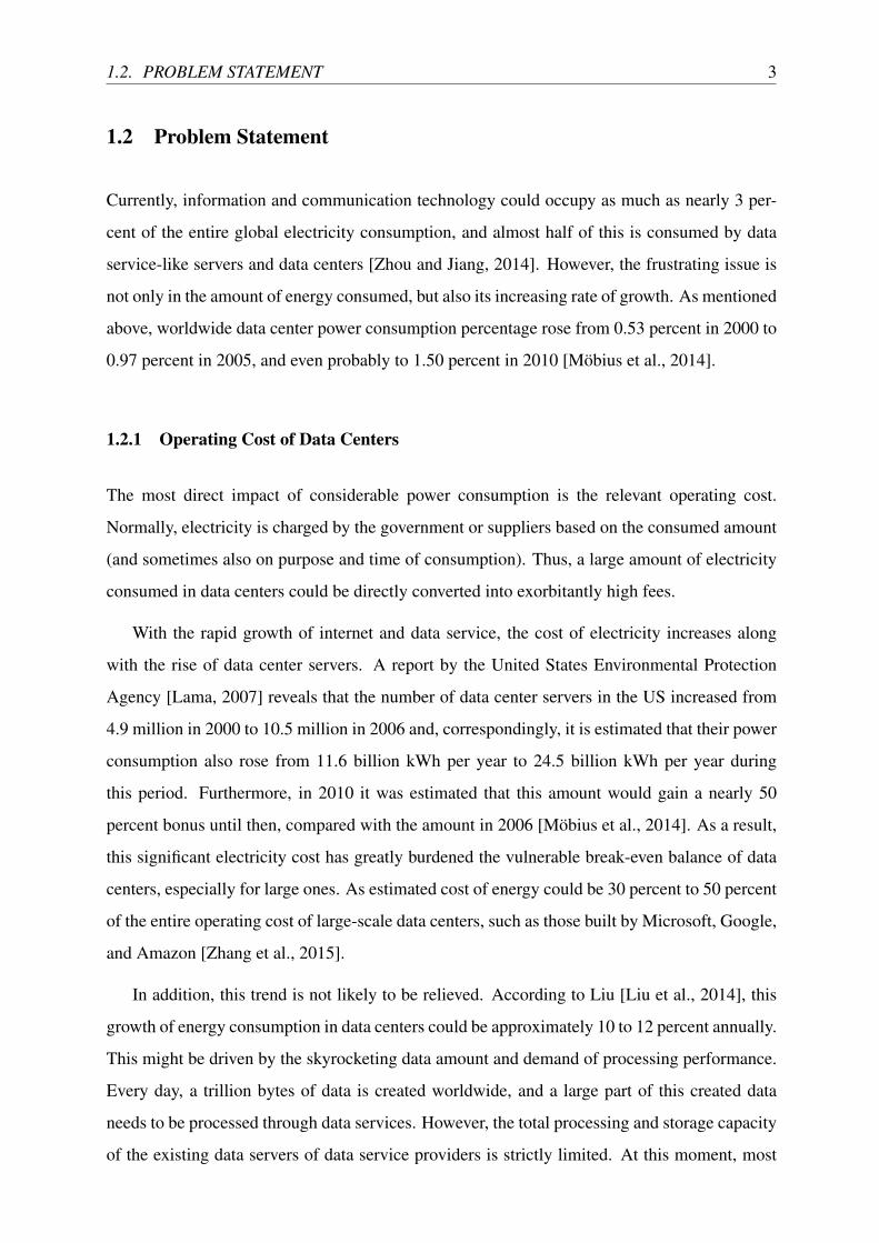
1.2.1 Operating Cost of Data Centers
The most direct impact of considerable power consumption is the relevant operating cost.
Normally, electricity is charged by the government or suppliers based on the consumed amount
(and sometimes also on purpose and time of consumption). Thus, a large amount of electricity
consumed in data centers could be directly converted into exorbitantly high fees.
With the rapid growth of internet and data service, the cost of electricity increases along
with the rise of data center servers. A report by the United States Environmental Protection
Agency [Lama, 2007] reveals that the number of data center servers in the US increased from
4.9 million in 2000 to 10.5 million in 2006 and, correspondingly, it is estimated that their power
consumption also rose from 11.6 billion kWh per year to 24.5 billion kWh per year during
this period. Furthermore, in 2010 it was estimated that this amount would gain a nearly 50
percent bonus until then, compared with the amount in 2006 [Mobius et al., 2014]. As a result,
this significant electricity cost has greatly burdened the vulnerable break-even balance of data
centers, especially for large ones. As estimated cost of energy could be 30 percent to 50 percent
of the entire operating cost of large-scale data centers, such as those built by Microsoft, Google,
and Amazon [Zhang et al., 2015].
In addition, this trend is not likely to be relieved. According to Liu [Liu et al., 2014], this
growth of energy consumption in data centers could be approximately 10 to 12 percent annually.
This might be driven by the skyrocketing data amount and demand of processing performance.
Every day, a trillion bytes of data is created worldwide, and a large part of this created data
needs to be processed through data services. However, the total processing and storage capacity
of the existing data servers of data service providers is strictly limited. At this moment, most

4 CHAPTER 1. INTRODUCTION
providers choose to add servers to enlarge the data processing and storage capacity, rather than
increasing their capacity. Consequently, the power consumption, as well as the cost, keeps being
raised, along with the number of data servers being added every day.
1.2.2 Power Delivery Challenge
This huge power consumption does not only reflect on the bills, but also on the requirements
of power delivery infrastructure [Beloglazov et al., 2011]. Normally, according to McClurg
[McClurg et al., 2013], traditional power delivery methods might have a 10 percent power
conversion loss, which would be a great deal of cost for data centers consuming a vast amount
of electricity. Therefore, this drives engineers to develop delivery methods with better effi-
ciency, also at high cost. However, Candan, Shenoy, and Pilawa-Podgurski have cited that
power delivery efficiency would hardly reach 100 percent, for any method. Finally, this power
conversion loss would still burden the vulnerable break-even balance of data centers.
Moreover, McClurg [McClurg et al., 2013] also examined the reliability and maintenance
of power supply units (PSUs), finding it to be quite challenging in large-scale data centers.
Because all servers share the same line current in data centers as stacked server clusters, any
single malfunctioning server node may deprive the other servers in the same current. Hopefully
those other servers are able to be shut down in time. However, this would also result in a
temporary interruption in server operation. Unfortunately, if the action mentioned above is
not executed in time, a cascaded over-voltage condition may result. In this scenario, hardware
damage to the servers, as well as the data loss, may not be easily avoidable.
1.2.3 Cooling and Fireproofing Trouble
Challenges brought by this huge power consumption are also in the cooling and fireproofing
infrastructure [Beloglazov et al., 2011]. In a large-scale data center, thousands of stacked server
clusters keep running in a narrow and closed room. Because a large part of the power consumed
by the servers becomes heat and is emitted into the air, the whole data center could become a
stove filled with efficient heaters. This situation often challenges the air-conditioning and even
fireproofing infrastructure.
One serious cooling issue of data centers has been examined [Zhang et al., 2015]. As
1.2. PROBLEM STATEMENT 5
different positions in one server release different amounts of heat, the accuracy of detecting
the position of heat emission is critical to the cooling system in one data center. Actually,
according to Wangs article Wang et al. [2013], quite a lot of ineffective cooling has been
executed worldwide because of the failure of detecting the heat-emitting position or conducting
targeted cooling methods. For example, Wikipedia went down in July, 2010 because of the
failure of one cooling unit. This caused the relevant server to overheat and then the whole data
center was caught in a power outage. Wang emphasizes that, if accurate heat-emission detection
had been deployed, this nightmare would probably have been avoidable.
In addition, air-conditioning is another issue that could increase the electricity bills of data
centers. It could be almost half of the entire energy consumption of data centers [Mobius et al.,
2014]. This is just the best case scenario. A cooling failure or a fire would cause even higher
costs, probably along with temporary service interruption and data loss.
1.2.4 Negative Environment Impacts
Apart from the operating cost and total cost of acquisition, huge electricity consumption has
also raised another urgent concern C its negative impact on the Earth [Beloglazov et al., 2011].
In most cases, the electricity-generating process often produces the emission of carbon dioxide,
which is strongly associated with the greenhouse effect. With such a huge amount of electricity
being consumed by data centers, a considerable amount of carbon dioxide has already been,
and is still being, released into the Earths atmosphere.
Furthermore, in generating such a huge amount of electricity, an extreme amount of fossil
fuels are dig up and burnt. Although the existing amount of those fuels is limited, the demand
for electricity by data centers is still growing. Probably in the near future, humans may finally
not afford the data created by them.
6 CHAPTER 1. INTRODUCTION
1.3 Technical Gaps
1.3.1 Technical Gaps
Researchers are already aware of the problem of huge power consumption by data centers
and have developed numerous methodologies to solve this problem, such as workload bal-
ancing, First Fit Decrease (FFD) algorithm, and Best Fit Decrease (BFD) algorithm. Each
methodology has been claimed in many published papers to have achieved greater energy
efficiency. However, after a survey on some recent virtualization platforms [Beloglazov et al.,
2011, Kajamoideen and Sivaraman, 2014], none of those methodologies have been implemented
in their hypervissr system or data centers. Both Xen and VMware are still using the easiest
onCoff switching and Dynamic Voltage and Frequency Scaling (DVFS) technology in physical
machine (PM) level for power efficiency, rather than any advanced virtual machine (VM)
placement methodologies in VM level.
Therefore, a VM-level placement framework, which is implementable, still needs to be
developed. Based on recent research, VM level will save at least 10 percent total energy
consumption [Liu et al., 2015, Luo et al., 2014, Mishra et al., 2012, Thraves and Wang, 2014,
Zhao and Liu, 2015].
In addition, none of the mentioned research achievements have applied the running records
of data centers to their methodologies. As big-data infrastructure, data centers running logs will
also be used as a big-data resource. Thus, the research in this thesis introduces profiles based
on those running records of data centers to the VM placement framework in order to optimize
the power efficiency.
Last but not least, there are often some permanent jobs running in data centers. These
jobs , such as mail service and the hypervisor system itself run continuously. However, recent
power-aware research or commercial implementation has not considered such situations. Those
existing resource-allocation strategies mix such permanent jobs with other jobs to conduct the
allocation of energy usage. As a result, those jobs will be distributed in far more PMs, than if
they were allocated together in a few high-power-efficiency machines. This mixture will not
guarantee SLAs and may even cost more in terms of energy.
1.4. RESEARCH OBJECTIVES AND CONTRIBUTIONS 7
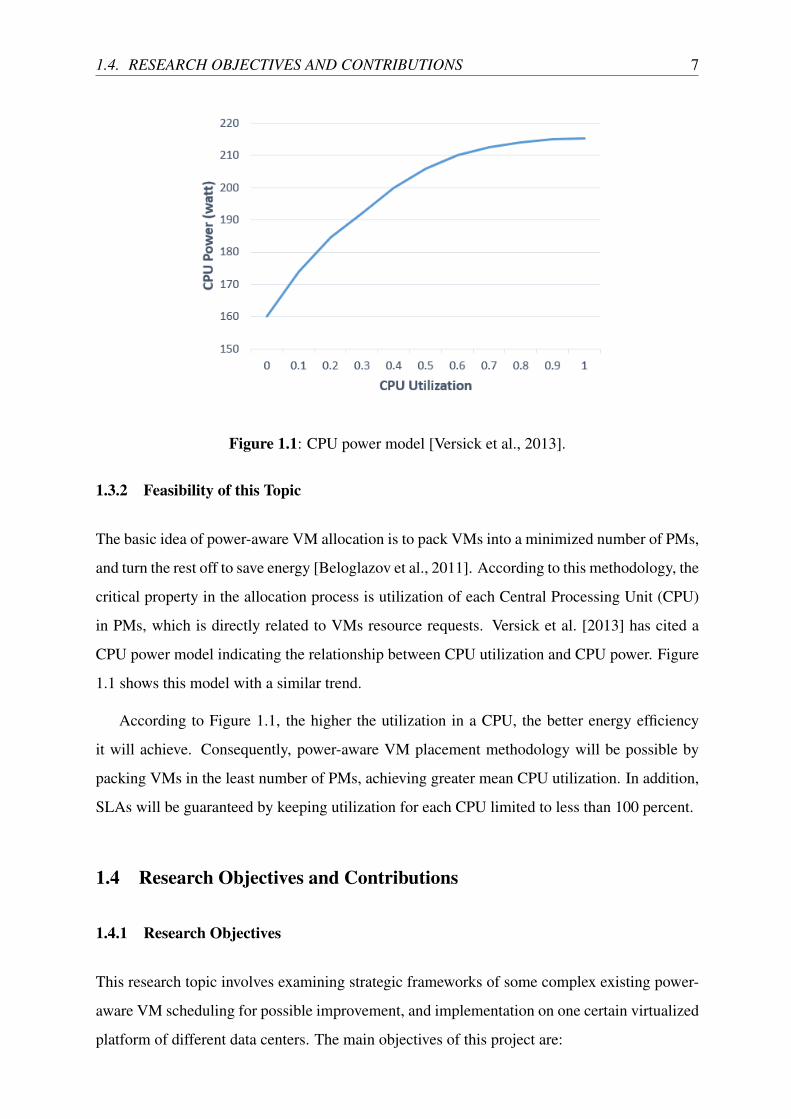
Figure 1.1: CPU power model [Versick et al., 2013].
1.3.2 Feasibility of this Topic
The basic idea of power-aware VM allocation is to pack VMs into a minimized number of PMs,
and turn the rest off to save energy [Beloglazov et al., 2011]. According to this methodology, the
critical property in the allocation process is utilization of each Central Processing Unit (CPU)
in PMs, which is directly related to VMs resource requests. Versick et al. [2013] has cited a
CPU power model indicating the relationship between CPU utilization and CPU power. Figure
1.1 shows this model with a similar trend.
According to Figure 1.1, the higher the utilization in a CPU, the better energy efficiency
it will achieve. Consequently, power-aware VM placement methodology will be possible by
packing VMs in the least number of PMs, achieving greater mean CPU utilization. In addition,
SLAs will be guaranteed by keeping utilization for each CPU limited to less than 100 percent.
1.4 Research Objectives and Contributions
1.4.1 Research Objectives
This research topic involves examining strategic frameworks of some complex existing power-
aware VM scheduling for possible improvement, and implementation on one certain virtualized
platform of different data centers. The main objectives of this project are:
8 CHAPTER 1. INTRODUCTION
1. To form and build profiles for VM placement for power-aware VM-placement methodol-
ogy
2. To classify tasks into appropriate sorts to help improve power-aware VM placement
3. To place VMs according to the results of profiling and classification results to achieve
better energy efficiency.
According to these objectives, this research aims to examine the power efficiency of some
VM scheduling strategies and frameworks for improvement. More specifically, in the future,
this research aims to develop and implement one optimized profile-based framework in one
certain virtual environment hypervising system.
1.4.2 Research Contributions
This thesis aims to formulate and deliver a new VM placement framework using profiling
methodology for energy optimization in data centers. This framework includes three stages:
profiling, VM classification, and VM placement. Through deployment of this framework, a
data center will achieve better energy efficiency with less migrations and guaranteed SLAs.
The first contribution of this thesis is that it introduces a profile-based methodology to VM
placement problems. By collecting and analyzing existing VM records of a data center, the
administration system will build profiles, which include critical information to help placing
VMs. Through profiles, administrators gain adequate ideas such as total CPU resource request,
number of jobs in each measurement period, and number of PMs needed.
The second contribution of this thesis is that it applies a task classification methodology
into the VM placement process. This methodology contributes to identifying different tasks by
typical characteristics and assigning these tasks into different VMs to enhance energy efficiency.
The third contribution of this thesis is that it develops a VM placement framework com-
bining the last two contributions and first fit decrease (FFD) algorithm. This framework limits
potential migrations and keeps a higher SLA. In addition, the framework also helps reduce
power consumption in data centers.

1.5. THESIS ORGANIZATION 9
1.5 Thesis Organization
Chapter 2 includes relevant literature reviews for this thesis, introducing recent developments
in the field of power-aware VM placement. Chapter 3 displays the formulation of the research
problem. Then the paper describes the three stages of the VM placement framework in Chapters
4, 5, and 6. In these three chapters, each stage identifiesobjectives, design, and experiments.
Finally, Chapter 7 concludes this framework with recommendations and future work require-
ments.

10 CHAPTER 1. INTRODUCTION
Chapter 2
Literature Review
With the skyrocketing requirements of data centers in almost all industries due to internet usage,
virtualized data centers, which could be more advanced in system and resource utilization and
flexibility, started to rapidly spread worldwide over the past decade [Lama, 2007].Virtualization,
the foundation theory of those virtualized data centers, has been improved over nearly half a
century, distributed by IBM, Xerox PARC, Sun, and nowadays almost all computing-related
companies [Douglis and Krieger, 2013]. It has been one of the most frequently debated topics,
mainly in relation to computing. With the help of virtualization technology, a data center could
be described as one computer directly offered to customers, forming the infrastructure as a
service (IaaS) level of Cloud computing as commercial use, and creating billions of dollars of
revenue annually worldwide [Buyya et al., 2010].
2.1 Virtualization Technology
Probably since the late 1960s, we have been exploring and developing the field of virtualization,
and nowadays, according to Williams [Williams, 2007], virtualization could be defined as:
1. A framework or methodology of dividing the resources of a computer hardware into
multiple execution environments, by applying one or more concepts or technologies
such as hardware and software partitioning, time sharing, partial or complete machine
simulation, emulation, quality of service, and many others.
11
12 CHAPTER 2. LITERATURE REVIEW
To briefly describe virtualization, it could be also perceived as an additional layer of abstrac-
tion between the application layer and the hardware layer, according to Williams [Williams,
2007]. Virtualization technology can use one or multiple combined physical computers to
form a computing resource pool for optimized resource allocation. Multiple parallel operating
systems (virtual machines, VMs) could run in this resource pool flexibly without considerable
waste of computing resources, compared with running in isolated single physical machines
(PMs).
In other words, virtualization is probably one indirect solution to some computing problems
in a different layer [Douglis and Krieger, 2013]. For instance, virtualization technology could
be beneficial for multiple upcoming applications for one computing system by forming homol-
ogous multiple VMs. For each application, based on each demand, the appropriate amount
of resources, such as CPU capacity, memory, storage, and network, would be extracted from
the resource pool. Thus, one certain VM would be formed to suit each application, as well as
one appropriate operating system. Finally, users could employ their applications for their own
clients independently via a network linked to this computing system, regardless of any direct
consideration or concern about the infrastructure.
Although a VM might be the most commonly known example of virtualization technology,
remote desktop sharing (virtual network computing, VNC), virtual networks (Cloud comput-
ing), and virtual storage (block virtualization) are also highly effective virtualization technology
implementations. Virtualization technology has strongly enhanced addressing myriad comput-
ing problems with efficiency, security, high availability, elasticity, fault containment, mobility,
and scalability [Douglis and Krieger, 2013].
2.2 Virtual Machine
Generally, a VM is defined as a self-contained operating environment created by one software
layer that behaves as if it were a separate computer[Matlis, 2006]. In other words, one VM
runs one independent operating system in the upper layer, which is isolated from physical
infrastructure or the existing operating system. It extracts the existing computing resource and
isolates a particular activity or application.
A VM is a computing environment on top of some other computing resources [Matlis, 2006].
2.2. VIRTUAL MACHINE 13
It is delivered to the user directly, regardless of the infrastructure. This feature significantly
stimulates the usability of computing resources, especially for remote users via the internet or
a local network, because the operating system of the ordered computing resource is already
on their screens (also with the help of VNC mentioned above). Thus, without worrying about
the power supply, cables, placement, and other possible management issues, users can simply
conduct computing tasks on the provided VMs. Recently, Amazon EC2 and Microsoft Azure
have both developed excellent service products in this field and have gained a high number
of loyal customers. Moreover, other companies, such as Google, Yahoo, and IBM, are also
promoting their own service products in the same field [Buyya et al., 2010].
The location of the layer of the VM often determines its purpose. Typically, if the layer of
one VM is above the operation system, it would isolate certain performances or applications. In
this case, VMs are often regarded as a desirable method ro avoid cross-corruption or other rele-
vant compiling problems, and probably for better user experience. This is usually implemented
in single computers.
In addition, if the layer of the VM is between the infrastructure and the operating system,
it would extract or combine existing computing resources. In this case, VMs are often used for
better resource utilization and elasticity. This is usually implemented in data centers to achieve
better computing resource administration, and to avoid the fact that users applications would be
restricted in single physical computers with idle or inadequate computing resources.
According to Matlis [Matlis, 2006], based on the location of the layer and the purpose
of VMs, there might be three different types of VMs, as hosted VMs, hypervisor VMs, and
application-level VMs.
2.2.1 Hosted VMs
Hosted VMs mainly refer to the VMs running guest operating systems as applications above
some existing host operating systems. Normally there would be an intermediary layer between
the host operating system and the guest operating systems. Thus, for one hosted VM, there
would be three components C an intermediary software layer, a guest operating system, and
most likely applications running the guest operating system.
Hosted VMs have numerous advantages, such as establishing another type of environment

14 CHAPTER 2. LITERATURE REVIEW
on the operating system instead of restarting the computer, allowing users to achieve legacy
programs or to partition an application from the rest of the system, and form a layer of protection
when conducting risky tasks.
2.2.2 Application-level VMs
Application-level VMs, especially the Java VM, is similar to hosted VMs as they also run on
an existing host operating system. However, application-level VMs combine the intermediary
software layer with the guest operating system, as it might not be necessary to directly provide
the guest operating system to users. Applications could run on the VMs. Traditionally, these
applications (like Java applications) are designed to only run on these VMs (like Java VM) to
avoid problems such as cross-corruption, lack of inter-layer communication mask, and flexible
resource allocation.
For example, Breg and Polychronopoulos [Breg and Polychronopoulos, 2001] have indi-
cated that the remote method invocation facility provided by the Java runtime environment
would allow Java objects to communicate in separate VMs. This facility could hide low-
level communication issues from the programmer, allowing them to focus on the distributed
algorithm instead. However, without the Java VMs, such communication should be directly
processed at the same layer as the program itself. This would strongly disturb programmers
when developing the programs.
2.2.3 Hypervisor VMs
Hypervisor (or hardware-level) VMs mainly refer to the VMs (or operating systems) built on
the hypervisor layer between the hardware and the operating systems. In this situation, each
operating system would regard itself as running under a standard configuration, but above
the hypervisor layer. The hypervisor centralizes the computing resources of the underlying
hardware and then allocates them to each VM.
Different from hosted VMs and application-level VMs, hypervisor VMs focus more on
performance rather than functions. As mentioned above, they could extract computing resources
from the infrastructure. Without the resource consumption of one other operating system and
possibly other applications on the same or lower layer, hypervisor VMs are usually more
2.3. VM MANAGEMENT 15
powerful and efficient than hosted VMs and application-level VMs. Therefore, they could
focus on providing better computing performance based on the specific demand of the given
application or task.
Furthermore, hypervisor VMs concentrate and reallocate physical computing resources.
This means that distributed computing systems, especially data centers, could achieve greater
computing resource utilization and elasticity by implementing hypervisor software. Conse-
quently, the system utilization of each physical computer would be nearly 100 percent or zero
(off) in the data center, and this would also help to achieve energy optimization by shutting
down more physical machines where no VMs are running [Beloglazov et al., 2011].
In summary, hosted VMs and application-level VMs are more function-aware VMs and
are mainly deployed in small-scale systems, such as single personal computers. However,
jypervisor VMs are more performance-aware and utilization-aware, and have already been
deployed in most existing data centers. All of these three types of VMs are beneficial to users
and infrastructure holders, as a part of virtualization technology. This topic (Virtual Machine
Scheduling for Energy Optimization of Data Centers) mainly discusses data centers deploying
large-scale hypervisor VMs.
2.3 VM Management
Virtualization technology is often associated with some special computing service. For exam-
ple, large-scale hypervisor VMs in data centers are often related to Cloud computing services,
and this is the focus of the research topic in this paper. Based on a marketing theory [Dickson,
2015], service improvement, through management, could be critical to the long-term survival,
evolution, and growth of one organization. Similarly, as a part of a computing service, it is also
necessary for VMs to be improved through proper management methods.
Normally, in data centers, VMs are monitored and managed by virtual machine monitors
(VMMs), also called hypervisors [Mishra et al., 2012]. A number of properties are required to
be monitored, such as the locating details (usually described as the IP address of the PM where
the VM is running), system utilization parameters (CPU, memory, storage, etc.), and computing
task circumstances (such as the recently achieved percentage, and predicted system utilization
requirement). Then, according to these properties, the VMM would probably optimize the entire
16 CHAPTER 2. LITERATURE REVIEW
workload by positioning each VM properly and allocating appropriate computing resources to
them.
In addition, the purpose of VM management most likely lies in the purpose of achieving
better quality of service (QoS) and service level agreements (SLAs) [Mishra et al., 2012].
In addition, these two items are often described as better performance, flexibility, and energy
efficiency. Therefore, the achievements of VM management should be adequately specialized
and examined. VM management mainly involves these three following measures C onCoff
switching, computing resource allocation, and migration. Each of them are necessary to VMs
for better QoS and are briefly discussed below.
2.3.1 OnCOff Switching
OnCoff switching, usually, is the most foundational function of VM management. This refers
to the action of creating and switching on one VM when required, as well as switching it off
and releasing the computing resource when the application running on it is terminated. In most
cases, this action is processed automatically by VMMs, as this is often essential, when required,
and could be processed by code work.
2.3.2 Computing Resource Allocation
Every VM, indeed, occupies a certain sum of computing resource (CPU performance, memory,
and storage space, etc.). Thus, such resources, when the VM is being created, must be allo-
cated to each VM through this computing resource allocation process. Basically, the allocated
resources are based on the coming workload of the application or computing task that would be
running on this VM. However, the forthcoming workload of applications and tasks is not easy
to predict accurately as it is usually dynamic. As a result, it is almost impossible to accurately
allocate computing resources to one VM only once from creating it to switching it off.
Due to this problem, much work has been done to improve the accuracy and efficiency of
computing resource allocation, including discussion of a possible resolution on Xen platform
in some articles [Minarolli and Freisleben, 2011]. This resolution mainly refers to the method
of allocating resources based on dynamic system utilization. The architecture mainly includes
2.3. VM MANAGEMENT 17
local controllers for each Xen hypervisor, and a global controller managing them. Local con-
trollers collect the recent workload as well as a historical log of each VM running on its relevant
Xen hypervisor, and then send them to the global controller. Researchers have also indicated
that the global controller would then analyse the entire workload, reallocate the computing
resources, and send commands back to local controllers. Finally, local controllers would imple-
ment the received commands to achieve better computing performance and sometimes energy
optimization.
The basic thinking of the reallocation of the global controller is to keep the system utilization
(mainly discussed as CPU utilization) of each VM at a proper stage, which often refers to
the stage near to but never reaching 100 percent. Normally, VMs at such system utilization
would gain the best performance with the least computing resources and power consumption.
This situation could just match the main purpose of virtualization technology, and also be
considerably beneficial.
2.3.3 VM Migration
VM migration is another effective method of VM management for better performance, flexi-
bility, and energy efficiency [Ahmad et al., 2015]. VM migration mainly refers to the action
of migrating one VM into a different location (PM). The purpose of VM migration is based
on the consideration of the workload of PMs associated with VM performance and energy
optimization. Commonly, each PM has its own workload as does each VM. Therefore, possible
measures could be conducted with PMs based on their workloads.
Based on the consideration of optimising VM performance, probably as well as the physical
limitation of the utilization of PMs, VM migrations happen when the utilization of one PM
reaches 100 percent [Malleswari et al., 2015]. At this time, no further computing resource could
be supplied from this machine because of the possible increase in resource demand of the VMs
running on it. As a result, sometimes some VMs have to be migrated from this fully utilized
PM to some other PMs where idle computing resources are still available. Consequently, the
performance of VMs cannot be restricted by the limitation of PM workloads, and users would
gain a better and smoother experience with more fluent service.
Much work has been done in this field also. For instance, Sato, Samejima, and Komoda
[Sato et al., 2013] have developed a dynamic placing method of VMs based on the resource
18 CHAPTER 2. LITERATURE REVIEW
utilization prediction. This method takes many more factors, such as time, energy consump-
tion, workload prediction, and first placement, into consideration. However, the accuracy
and reaction speed are not appropriate enough, because of the complexity of the prediction.
Consequently, it is likely that still more work is needed in this field.
In addition, based on the consideration of optimizing energy consumption, VM migrations
happen when the utilization of one physical machine reaches quite a low level, such as 50
or 40 percent. Currently, most power consumed by this PM is for the basic demand of its
hardware, regardless of supply to the VMs. This situation is often considered as a waste of
power [Beloglazov et al., 2011]. Therefore, VMs on such PMs are often asked to migrate,
possibly to other PMs that could reach more appropriate utilization, such as, for example, 90
percent. Those PMs from which VMs have migrated away could then be shut down, as a
switched-off computer would cost almost no electricity. This situation is discussed in more
detail in the next chapter.
In summary, correct methods of VM management, including onCoff switching, computing
resource allocation, and migration are often necessary to achieve better QoS and SLAs. How-
ever, methods for better energy efficiency are more concentrated.
2.4 Green Cloud Architecture
As mentioned in Chapter 1, the aim of this research topic is to address the existing VM schedul-
ing methods that lead to Green Cloud computing in data centers [Monteiro et al., 2014], in
order to satisfy competing applications requirement for computing services and save energy.
It is sited the high-level architecture for supporting energy-efficient service allocation in Green
Cloud computing infrastructure [Buyya et al., 2010]. There are foundationally four main entities
involved in this architecture.
1. Consumers and brokers: Cloud consumers and their brokers submit service requests from
anywhere in the world to the Cloud. Actually, this group are rarely concerned about
energy consumption, instead focusing on user experience, processing performance, and
service reliability.
2. Green resource allocator: This allocation acts as the interface between the consumers and
brokers and the Cloud infrastructure. There are two sorts of interface C the consumer
2.5. VM SCHEDULING STRATEGIES 19
interface and the Cloud interface. The consumer interface involves elements as green
negotiator, service analyzer, consumer profiler, and pricing. This interface is directly
linked to the consumers and brokers. In addition, the Cloud interface involves elements
such as energy monitor, service scheduler, VM manager, and accounting. This interface
is linked to the VMs, acting as VMMs, and some other infrastructure management role.
3. VMs: As introduced earlier in this chapter, VMs could be started and stopped dynami-
cally in one or a sort of PMs to provide maximum flexibility to configure various partitions
of resources to different specific requirements of service requests. Moreover, multiple
VMs could concurrently process different applications within different computing envi-
ronments. In addition, by dynamically migrating VMs across PMs, workloads could be
consolidated, and unused resources could be switched off or kept on a low-power state
for the purpose of energy optimization.
4. Physical Machines: The underlying physical computing servers provide hardware infras-
tructure for creating virtualized resources to meet service demands, supported by other
subsidiary infrastructure, such as air-conditioning and fireproofing.
This Green Cloud architecture would meet the performance and reliability demand as well as
the energy-optimizing requirement with adequate concern for the energy efficiency management
of applications, VMs, and PMs.
This research topic (Virtual Machine Scheduling for Energy Optimization of Data Centers)
mainly explores the green resource allocator part of the Green Cloud architecture, especially
the elements involved in the Cloud interface.
2.5 VM Scheduling Strategies
Recently, many researchers have tended to apply workload balance to energy control. Luo et al.
[2014] recommends deploying such methodology through a workload-shaping and queuing-
delay concept. He also built up a real-life-based electricity price model with enterprise-level
workload distribution. He finally achieved a certain power reduction, but with a high risk of
unexpected workload drop. In addition, this methodology did not reduce the number of running
servers, unlike other VM scheduling algorithms. Moreover, Yu et al. [2015] has made similar
20 CHAPTER 2. LITERATURE REVIEW
efforts through the concept of workload balance to limit power consumption in data centers.
However, he did not solve the problem of PM numbers as well. Workload balance is more
suitable for guaranteeing SLAs in data centers[Zhao et al., 2013], rather than focusing on energy
optimization only.
FFD is a common algorithm dealing with bin-packing problems, and VM placement is
just such a problem [Thraves and Wang, 2014]. Zhao and Liu [2015] has implemented an
advanced FFD algorithm in VM placement problems. However, he did not solve the power
consumption problem through FFD algorithm. On the other hand, Dai [Dai et al., 2016] recently
introduced such methodology against a greedy algorithm. Almost 50 per cent of energy was
saved compared with the original greedy algorithm. However, this allocation algorithm could
have been improved if Dai had deployed more VM profiles, such as classification.
BFD is another algorithm dealing with bin-packing problems, and its results are often better
than FFD algorithm. Liu et al. [2015] has implemented this algorithm into VM placement
for energy optimization problems. The BFD algorithm in that paper is based on the resource
utilization ratio rather than real utilization numbers. This makes it difficult to deploy this idea
into real data centers, especially with different server configurations.
Moreover, Lama Lama [2007] has introduced GA algorithm to this area. However, GA
algorithm fits a long-lasting dynamic placement problem. When there are numerous scheduled
VMs to submit in a data center, GA algorithm cannot offer a high-performance allocation plan
in a short execution time. In addition, this research did not include any valuable VM profiles at
all.
Besides any methodology research, some researchers did study whether it would be worth
exploring this field further. Graubner et al. [2013] did a study on energy-oriented VM con-
solidation. This paper indicates that VM consolidation did save power during operation of the
π-estimation benchmark program. In addition, the execution time did not greatly changed when
VM consolidation was deployed. The result gives confidence to do further research in the field
of energy-aware VM placement.
2.6. SPECIFIC VM SCHEDULING SCHEMES 21
2.6 Specific VM Scheduling Schemes
VM management for energy optimization is a very important section of the Green Cloud archi-
tecture. It aims to schedule and allocate VMs properly for minimum power consumption and
appropriate performance and reliability. By conducting excellent VM scheduling work, VMs in
one data center would run smoothly, as well as having a low power ratio. There are at least four
strategies of VM scheduling for this purpose.
1. Focus on system utilization: According to Buyya et al. [2010] and Beloglazov et al.
[2011], for one PM, which is the real entity of power consumption, the higher the system
utilization, the better energy efficiency it would reach. This is because the lower the
system utilization, the less percentage of electricity this PM could use to achieve data
processing, regardless of an almost static amount of power for just keeping the hardware
operating. In addition, if the workload of one PM is always 100 percent, this might have
a negative effect on dynamic tasks or applications running on its relevant VMs, for some
tasks or applications may suddenly request more computing resources. As a result, it is
ideal to keep all PMs running between a high threshold and a low threshold, to maintain
the best reliability and energy efficiency balance.
2. Minimize running physical machines: Based on the previous strategy, the workload of
both VMs and PMs should always be monitored [Graubner et al., 2013]. Based on the
monitoring result, VMs running on PMs with low system utilization could be gathered
to achieve higher system utilization in fewer PMs. At present, the PMs where no VM is
running could be switched off to save energy. Consequently, for a certain number of VMs,
the number of running PMs would be minimized to achieve both high system utilization
and appropriate energy efficiency.
3. Minimize migrations: During migration of one VM, both the source and destination PM
should be kept on, allocating the same adequate computing resources for this VM. It could
be considered as that this VM at least doubles its power ratio. Therefore, migrations
should be minimized. In other words, each migration should be executed with careful
consideration of the energy-efficiency risks [Buyya et al., 2010]. In addition, unnecessary
migration should usually be prohibited to save power.
4. Predict future workload: As most of the tasks and applications running on VMs change

22 CHAPTER 2. LITERATURE REVIEW
dynamically, it is necessary to allocate adequate resources before the changes happen.
With accurate and effective prediction of the future workload of one VM, proper com-
puting resources could be allocated to it for an improved user experience; unnecessary
migration might be avoided by a long-lasting placement. However, accurate prediction
still requires quite much work. The recent strategy of predicting workload is to have a
pilot process for a certain period to assess the future workload of one VM.
As energy efficiency is topic of real-world relevance, any possible factors and strategies
should be also seriously examined. However, other factors and strategies are beyond the means
of this paper.
2.7 Recent Commercial Implementation
Recently, many open-source and commercial virtualization systems have taken consideration of
energy-aware VM management, such as Xen and VMware. Both have implemented subsystems
or functions of their hypervisors to gain the VM power-controlling functions. It The article by
Beloglazov [Beloglazov et al., 2011]has introduced both of their power management functions.
2.7.1 Xen
The Xen hypervisor is an open-source virtualization technology developed collaboratively by
the Xen community and engineers from over twenty innovative data center solution vendors
[Beloglazov et al., 2011]. Xen enables the switching between P-states (power-performance
states) and C-states (CPU sleeping states), both of which are quite beneficial to the energy
efficiency of the object-virtualized system. In addition, Xen provides the four following power
management governors within a subsystem.
1. Ondemand: This governor would choose the best P-state, according to current resource
requirements.
2. Userspace: This governor would set the CPU frequency, which is related to the power
ratio specified by the user.
3. Performance: This governor would set the highest available clock frequency for the best
performance, regardless of energy saving.
2.8. PROFILES 23
4. Powersave: This governor would set the lowest clock frequency for better power ratio.
Moreover, besides P-states and C-states, Xen also provides regular and live migration,
which could be leveraged by power-aware dynamic VM consolidation algorithms. This process
would generally follow the VM scheduling strategies mentioned above to achieve better energy
efficiency with appropriate performance.
2.7.2 VMware
VMware, Inc. has provided vSphere (VMware ESXi) to support enterprise-level virtualization
solutions. For energy efficiency, vSphere supports dynamic voltage and frequency scaling
(DVFS) technology to adjust the CPU voltage as well as its frequency related to the voltage
to meet the demand of performance or power ratio. In addition, vSphere also provides a
VMotion and VMware Distributed Resource Scheduler (DRS) to enable the live migration of
VMs. VMware DRS could monitor the computing resource utilization in the resource pool and,
if necessary, use VMotion to conduct a live migration according to current workload and power
balance policy.
Moreover, VMware DRS also contains a subsystem called VMware Distributed Power
Management (DPM). VMware DPM could switch off the idle servers according to the current
monitoring result from VMware DRS to achieve better energy efficiency.
2.8 Profiles
Google Cluster-Usage Traces version 2 [Reiss et al., 2011] are configuration traces about a
Google cluster for around one month. These traces were released in 2011 by Google. They
are formed by racked machines, which are connected by a cluster network. Normally machines
are packed into cells, which are used as destinations for incoming jobs. Each job may include
one or more tasks as Linux programs relatively, and finally each task is assigned to only one
machine for processing. By addressing a typical VM according to each tasks request, this data
set could be regarded as a VM profile in one virtualized data center.
The whole data set includes different tables about machines, and jobs and tasks. In each of
the parts, it demonstrates almost all necessary information of each VM or PM, in all relevant
24 CHAPTER 2. LITERATURE REVIEW
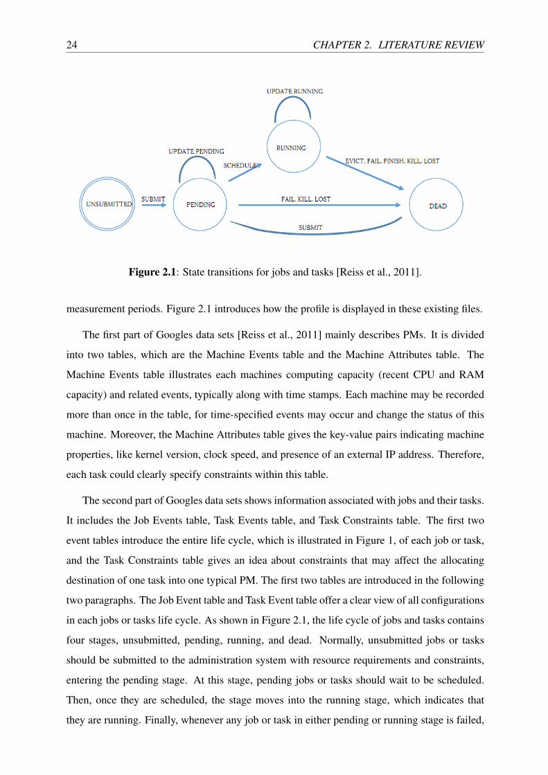
Figure 2.1: State transitions for jobs and tasks [Reiss et al., 2011].
measurement periods. Figure 2.1 introduces how the profile is displayed in these existing files.
The first part of Googles data sets [Reiss et al., 2011] mainly describes PMs. It is divided
into two tables, which are the Machine Events table and the Machine Attributes table. The
Machine Events table illustrates each machines computing capacity (recent CPU and RAM
capacity) and related events, typically along with time stamps. Each machine may be recorded
more than once in the table, for time-specified events may occur and change the status of this
machine. Moreover, the Machine Attributes table gives the key-value pairs indicating machine
properties, like kernel version, clock speed, and presence of an external IP address. Therefore,
each task could clearly specify constraints within this table.
The second part of Googles data sets shows information associated with jobs and their tasks.
It includes the Job Events table, Task Events table, and Task Constraints table. The first two
event tables introduce the entire life cycle, which is illustrated in Figure 1, of each job or task,
and the Task Constraints table gives an idea about constraints that may affect the allocating
destination of one task into one typical PM. The first two tables are introduced in the following
two paragraphs. The Job Event table and Task Event table offer a clear view of all configurations
in each jobs or tasks life cycle. As shown in Figure 2.1, the life cycle of jobs and tasks contains
four stages, unsubmitted, pending, running, and dead. Normally, unsubmitted jobs or tasks
should be submitted to the administration system with resource requirements and constraints,
entering the pending stage. At this stage, pending jobs or tasks should wait to be scheduled.
Then, once they are scheduled, the stage moves into the running stage, which indicates that
they are running. Finally, whenever any job or task in either pending or running stage is failed,
2.9. SUMMARY OF LITERATURE REVIEW 25
killed, lost, or finished, it enters the dead stage, in which each job or task should be dropped or
resubmitted.
In addition, the Job Event table and Task table record all relevant data in these stages, such
as time stamp, job or task ID, event type, scheduling class, computing resource requests (CPU,
RAM, and local disk space), and priority. According to these two tables, the system should be
able to assign every job or task into an appropriate machine.
Nevertheless, computing resources are still being consumed when jobs and tasks are run-
ning. As a result, another table records the timely resource usage of each task, called the
Resource Usage table. In this table, all tasks real resource consumption is recorded by mea-
surement periods. Normally one measurement period is around 300 seconds. However, as long
as tasks have start or end times different from fixed-measurement time stamps, the start or end
time of some tasks may be related to their real start or end time against a 300-second-cycle
time stamp. Moreover, this table records both mean and maximum CPU or RAM usages of all
tasks in each relevant measurement period. Consequently, system administrators or the system
itself could be provided with adequate runtime information for all jobs and tasks, which would
greatly help to improve allocation strategies and SLA.
In conclusion, the six tables mentioned above form Google Cluster-Usage Traces version 2.
Each of them collects significantly sufficient content of VM or PM information. In addition,
this data set will also be applied to the upcoming experiments in this thesis.
2.9 Summary of Literature Review
This chapter has cited recent literature reviewed by the author, including virtualization foun-
dation, VM management methodologies, power-aware data center management, and related
work by other researchers. This literature indicates that people are already sufficiently aware
of the incredible energy cost in data centers, and have made great efforts to solve this problem.
However, few solutions have been adopted by enterprises, and few researchers include VM pro-
files in this field. These facts urge a profile-based, deployable, power-aware VM management
framework to be developed and released.

26 CHAPTER 2. LITERATURE REVIEW
Chapter 3
Formulation and Design
Chapter 3 mainly discusses the formulation of the research questions for this paper. Since the
research questions focus on energy optimization, an energy consumption model is built for final
evaluation. In addition, the virtual machine (VM) placement models are also introduced for
future algorithm design and implementation. Finally, according to the two models demonstrated
in this chapter, the formalized goal of this research topic iss addressed for a better understanding
towards further research stages.
3.1 Energy Consumption Model
The energy consumption model here is used to evaluate the power efficiency of one VM place-
ment solution. In this model, the entire energy consumption of one data center, which will
be affected by the methods introduced in this paper, is calculated. Furthermore, each VM
placement plan should be related to one supposed energy consumption. Thus, by comparing
the energy consumption of each plan, the plan combined with least energy consumption will be
chosen as the best plan to implement.
Normally, the energy consumption in one data center includes a number of ingredients, such
as power costs for the physical macines (PMs), administration system, and air-conditioning
system. Regarding E for energy consumption, the energy consumption in one data center is
identified as:
EDataCenter = EPM + EAdminSystem + EAir−con + ... (3.1)
As power consumption for the administration system and air-conditioning system are almost
27
28 CHAPTER 3. FORMULATION AND DESIGN
fixed through VM placement plans, those ingredients will be omitted during evaluation, retain-
ing only the PMs power cost.
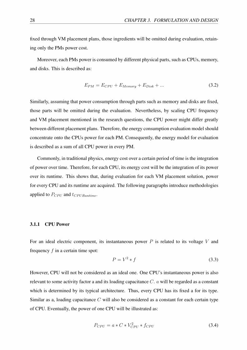
Moreover, each PMs power is consumed by different physical parts, such as CPUs, memory,
and disks. This is described as:
EPM = ECPU + EMemory + EDisk + ... (3.2)
Similarly, assuming that power consumption through parts such as memory and disks are fixed,
those parts will be omitted during the evaluation. Nevertheless, by scaling CPU frequency
and VM placement mentioned in the research questions, the CPU power might differ greatly
between different placement plans. Therefore, the energy consumption evaluation model should
concentrate onto the CPUs power for each PM. Consequently, the energy model for evaluation
is described as a sum of all CPU power in every PM.
Commonly, in traditional physics, energy cost over a certain period of time is the integration
of power over time. Therefore, for each CPU, its energy cost will be the integration of its power
over its runtime. This shows that, during evaluation for each VM placement solution, power
for every CPU and its runtime are acquired. The following paragraphs introduce methodologies
applied to PCPU and tCPURuntime.
3.1.1 CPU Power
For an ideal electric component, its instantaneous power P is related to its voltage V and
frequency f in a certain time spot:
P = V 2 ∗ f (3.3)
However, CPU will not be considered as an ideal one. One CPU’s instantaneous power is also
relevant to some activity factor a and its loading capacitance C. a will be regarded as a constant
which is determined by its typical architecture. Thus, every CPU has its fixed a for its type.
Similar as a, loading capacitance C will also be considered as a constant for each certain type
of CPU. Eventually, the power of one CPU will be illustrated as:
PCPU = a ∗ C ∗ V 2CPU ∗ fCPU (3.4)
3.1. ENERGY CONSUMPTION MODEL 29
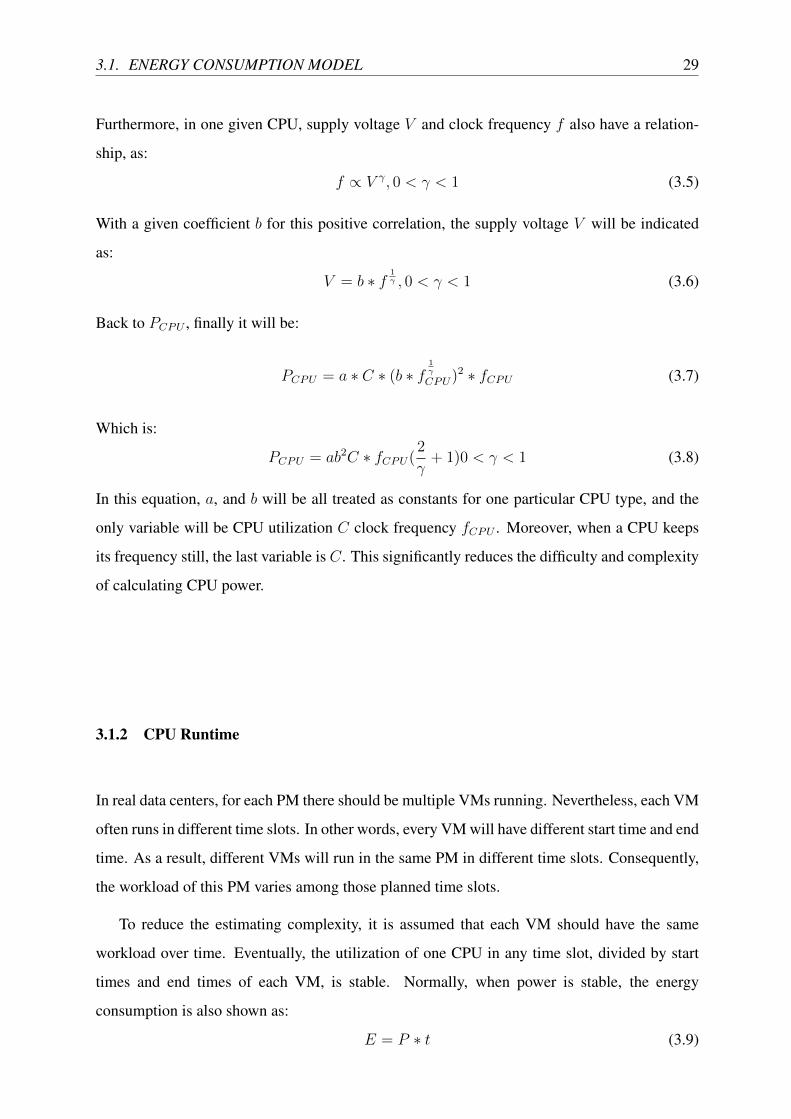
Furthermore, in one given CPU, supply voltage V and clock frequency f also have a relation-
ship, as:
f ∝ V γ, 0 < γ < 1 (3.5)
With a given coefficient b for this positive correlation, the supply voltage V will be indicated
as:
V = b ∗ f1γ , 0 < γ < 1 (3.6)
Back to PCPU , finally it will be:
PCPU = a ∗ C ∗ (b ∗ f1γ
CPU)2 ∗ fCPU (3.7)
Which is:
PCPU = ab2C ∗ fCPU(2
γ+ 1)0 < γ < 1 (3.8)
In this equation, a, and b will be all treated as constants for one particular CPU type, and the
only variable will be CPU utilization C clock frequency fCPU . Moreover, when a CPU keeps
its frequency still, the last variable is C. This significantly reduces the difficulty and complexity
of calculating CPU power.
3.1.2 CPU Runtime
In real data centers, for each PM there should be multiple VMs running. Nevertheless, each VM
often runs in different time slots. In other words, every VM will have different start time and end
time. As a result, different VMs will run in the same PM in different time slots. Consequently,
the workload of this PM varies among those planned time slots.
To reduce the estimating complexity, it is assumed that each VM should have the same
workload over time. Eventually, the utilization of one CPU in any time slot, divided by start
times and end times of each VM, is stable. Normally, when power is stable, the energy
consumption is also shown as:
E = P ∗ t (3.9)
30 CHAPTER 3. FORMULATION AND DESIGN
In this case, if one PM j is divided into K time slots, its energy consumption will be:
Ej =K∑k=1
(Pjk ∗ tjk) (3.10)
In this equation, Pjk stands for the instantaneous power of time slot k in PM j, and tjk stands
for the duration of this time slot.
3.1.3 Data Center Power Model
Finally, combining the results of both power and time together, the power consumption of PM
j is:
Ej =K∑k=1
[ab2C ∗ f( 2γ+1)
j ∗ tjk] (3.11)
Therefore, the entire energy consumption is:
E =n∑j=1
Ej (3.12)
Which is:
E =n∑j=1
{K∑k=1
[ab2C ∗ f( 2γ+1)
j ∗ tjk]} (3.13)
In this equation, n is the number of PMs that are switched on. For each VM placement plan,
one energy consumption figure is calculated. Thus, for plan p and plan q, if:
Ep > Eq (3.14)
This indicates that plan q is better than plan p in energy optimization. Otherwise, plan p will
be better. After analysing all placement plans, one or some best plans of energy optimization
should become apparent through an exhaustive comparison.
3.2 VM Placement Model
The VM placement model is used to mathematically define each placementt decision, as wellas
the final union of all single placement decisions.
3.3. ENERGY OPTIMIZATION OBJECTIVE 31
This has given a mathematical model for VMs. According to this model, the union of VM
is scheduling decisions will be:
opi = {p,m} (3.15)
opi is the scheduling decision for VM i. In addition, p is for the placement of this VM, and m
is the migration of it. As this paper focuses on placement measures, m will be always ∅ in this
paper.
Furthermore, the decision to unite all VMs in PM j is defined as:
OPj =⋃{opi} (3.16)
In addition, every VM always includes components: scheduling options op, resource request r,
start time tStart, end time tEnd, and the target node PM . Thus, one VM is defined as:
vmi = {op, r, tStart, tEnd, PM} (3.17)
Supposing there are m VMs in total, then all the VMs will be:
VM =⋃
1≤i≤m
{vmi} (3.18)
3.3 Energy Optimization Objective
The goal of this research topic is to find the best solution for multiple VM placement of energy
optimization with frequency scaling. In other words, this goal is to find a VM placement plan
combined with frequency scaling, to ascertain the least energy consumption. Thus, mathemati-
cally it is described as:
To find:
OP =⋃{OPj} (3.19)
Which will achieve:
minEOP =n∑j=1
{K∑k=1
[ab2C ∗ f( 2γ+1)
j ∗ tjk]} (3.20)
Subject to:
32 CHAPTER 3. FORMULATION AND DESIGN
1.
0 ≤ ulower ≤ ∀ujk ≤ uupper ≤ 100% (3.21)
2.
∀fj ∈ {F1, F2, F3, ..., Fq, 1 ≤ j ≤ n (3.22)
3.
0 ≤ ∀ujkmemory ≤ 100% (3.23)
Among these restrictions, first, to face the service level agreements (SLAs), the utilization
of any PM should be controlled between particular upper and lower thresholds. Whenever the
utilization is above the upper threshold, the CPU may not be capable of dealing with sudden
additional resource requests. In addition, whenever the utilization is below the lower threshold,
the energy efficiency will be too low to leave this PM running. Thus, it is necessary to keep
each PM running between the two thresholds.
Second, the frequency choices are limited. There are several recommended frequency levels
for each PM by the hypervisor. Therefore, the frequency decisions will be made among these
given frequency levels.
Last but not least, capacity of other physical components in a PM should also be considered.
For example, the memory utilization should never be above 100% through requests, as it is
physically impossible.
3.4 Framework Design
The goal of this research topic is to establish a VM placement framework, using profile, VM
classification, and FFD algorithm. Accordingly, the architecture design of this framework will
include these three ingredients. Therefore, the design contains three phases C profiling phase,
VM classification phase, and VM placement phase. The high-level architecture is illustrated in
Figure 3.1.
The first part of this framework is the profiling phase. The intent of this phase is to build
VM profiles and to identify each VMs runtime, resource requests, and previous utilizations. The
profiles are based on past VM logs and forthcoming VM plans. According to these profiles, the
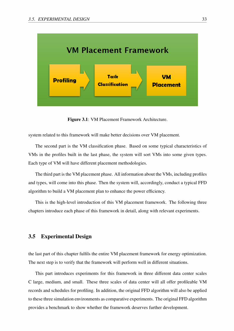
3.5. EXPERIMENTAL DESIGN 33
Figure 3.1: VM Placement Framework Architecture.
system related to this framework will make better decisions over VM placement.
The second part is the VM classification phase. Based on some typical characteristics of
VMs in the profiles built in the last phase, the system will sort VMs into some given types.
Each type of VM will have different placement methodologies.
The third part is the VM placement phase. All information about the VMs, including profiles
and types, will come into this phase. Then the system will, accordingly, conduct a typical FFD
algorithm to build a VM placement plan to enhance the power efficiency.
This is the high-level introduction of this VM placement framework. The following three
chapters introduce each phase of this framework in detail, along with relevant experiments.
3.5 Experimental Design
the last part of this chapter fulfils the entire VM placement framework for energy optimization.
The next step is to verify that the framework will perform well in different situations.
This part introduces experiments for this framework in three different data center scales
C large, medium, and small. These three scales of data center will all offer profileable VM
records and schedules for profiling. In addition, the original FFD algorithm will also be applied
to these three simulation environments as comparative experiments. The original FFD algorithm
provides a benchmark to show whether the framework deserves further development.

34 CHAPTER 3. FORMULATION AND DESIGN
Figure 3.2: Final Experimental Design
Experiments in this thesis determine to show the performance of the VM placement frame-
work in different data center scales, with the comparative target as the original FFD algorithm.
As shown in Figure 3.2, the experiments are designed as the same architecture as the framework,
including input, profiling, classification, placement, and evaluation. However, for the original
FFD algorithm, the profiling and classification section is omitted as there are no such sections
in its architecture.
In the input section, the input files include relevant files from Google Cluster-Usage Traces
[Reiss et al., 2011]. As the given Google data sets are data center records for one month, only
one record, for about 24 hours, has been extracted for these experiments. In addition, to fulfil
three different scales of data centers, a further extraction has been conducted. At first, to form
the large-scale data center, the experiment extracted one record for every 200 records from the
original record files. Then, an every-400 version and every-1000 version are also extracted
to form the medium- and small-scale data centers. However, as the related data center is a
non-virtualized data center [Reiss et al., 2011], some assumptions are necessary to fulfil the
experiments.
1. There are three new virtualized data centers in the three different scales.
2. All tasks recorded or scheduled are assigned to only one VM in each data center in each
measurement period.
3. The task records can be treated as forthcoming task schedules.
4. Googles data sets are used, as input files, only for testing the framework.
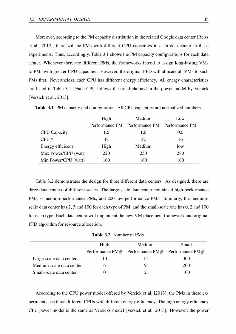
3.5. EXPERIMENTAL DESIGN 35
Moreover, according to the PM capacity distribution in the related Google data center [Reiss
et al., 2012], there will be PMs with different CPU capacities in each data center in these
experiments. Thus, accordingly, Table 3.1 shows the PM capacity configurations for each data
center. Whenever there are different PMs, the frameworks intend to assign long-lasting VMs
to PMs with greater CPU capacities. However, the original FFD will allocate all VMs to such
PMs first. Nevertheless, each CPU has different energy efficiency. All energy characteristics
are listed in Table 3.1. Each CPU follows the trend claimed in the power model by Versick
[Versick et al., 2013].
Table 3.1: PM capacity and configuration. All CPU capacities are normalized numbers.
High Medium LowPerformance PM Performance PM Performance PM
CPU Capacity 1.5 1.0 0.5CPU# 48 32 16Energy efficiceny High Medium lowMax Power/CPU (watt) 220 250 280Min Power/CPU (watt) 160 160 160
Table 3.2 demonstrates the design for three different data centers. As designed, there are
three data centers of different scales. The large-scale data center contains 4 high-performance
PMs, 6 medium-performance PMs, and 200 low-performance PMs. Similarly, the medium-
scale data center has 2, 3 and 100 for each type of PM, and the small-scale one has 0, 2 and 100
for each type. Each data center will implement the new VM placement framework and original
FFD algorithm for resource allocation.
Table 3.2: Number of PMs.
High Medium SmallPerformance PM# Performance PM# Performance PM#
Large-scale data center 10 15 300Medium-scale data center 6 9 200Small-scale data center 0 2 100
According to the CPU power model offered by Versick et al. [2013], the PMs in these ex-
periments use three different CPUs with different energy efficiency. The high energy efficiency
CPU power model is the same as Versicks model [Versick et al., 2013]. However, the power

36 CHAPTER 3. FORMULATION AND DESIGN
model of the other two CPUs are different from the model. Both of these two models keep
similar trends as the high energy efficiency CPU power model. The peak power of the medium
power efficiency CPU is designed as 250 watt, and low power efficiency CPU is 280 watt.
Therefore, these three kinds of CPU will have different energy efficiency.
Like Amazon EC2 Amazon-Web-Services [2016], the scales of VMs in a data center are
fixed as certain types. In Amazon EC2, users are only able to choose VMs with given fixed
configurations. Similarly, in the three data centers for the experiments, the VMs configurations
are also fixed. Table 3.3 lists all relevant VM configurations to be used in the experiments.
Table 3.3: VM configuration in normalized CPU capacity.
Huge VM Large VM Medium VM Normal VM Small VM Tiny VMCPU Capacity 0.45 0.3 0.15 0.1 0.045 0.015
Furthermore, experiments in this thesis are simulated in a desktop computer as a data center
environment. This simulation is conducted by a written program acting as a data center admin-
istration system. The program is written in Java (JKD 1.8.0.91). In addition, the deployment
environment is a desktop computer with Inter Core2 Q6700 3.4 GHz CPU and 32 GB DDR4
2666 MHz RAM, in Windows 10 professional operating system.
Finally, when all experiments are done, evaluation is necessary for verification. The eval-
uation section includes timely PM number, average PM utilization, total energy consumption,
and computing time evaluation. The methodology with fewer timely PMs, greater average PM
utilization, less total energy consumption, or less computing time, will be considered the better
one.
3.6 Chapter Summary
This chapter has offered the formulation of the research problem and objective. Then, according
to the formulation results, it gives the design of a new VM placement framework for energy op-
timization, including profiling, VM classification, and VM placement. Finally, the last section
has demonstrated the design of relevant experiments following each part of the framework. The
next three chapters will introduce each part of this framework one by one, followed by relevant
experiments.
Chapter 4
Profiling and Profile Building
Chapter 4 introduces the first part of the new VM placement framework, the profiling part. At
first, it shows a clear view of Google’s data sets, which will be used in all experiments. The
next section illustrates what information will be extracted from the original files to form profiles.
Then, the exact design of profiles are listed, and finally, relevant experiments and analysis are
cited for evaluation.
4.1 VM Profile
There are often some logs recording numerous typical details during the runtime of one estab-
lished data centre, including incoming VM requests, VM operation records, and PM operation
records. As a considerable way for resource management, many well-known enterprises have
already implemented profiling typical methodologies in their data centres.
For instance, VMware has deployed profiling methodology into its existing productions,
such as VMware work station and vSphere series [Kajamoideen and Sivaraman, 2014]. Accord-
ingly, VMware implements VM and PM configuration profiles to indicate flows of computing
resources or power consumption. In addition, those profiles are also used to predict future
resource allocation with incoming VM schedule acknowledgments.
Moreover, according to Google Cluster-Usage Traces [Reiss et al., 2011], Google has also
implemented profiling methodology tracing configurations of specified data centre components.
As mentioned in its documentation, these traces relate to a non-virtualized data centre.
By analyzing these records and extracting useful information from them, profiles shall be
37
38 CHAPTER 4. PROFILING AND PROFILE BUILDING
built, indicating what system and administrators need to know to enhance the performance of
data centre. For example, hypervisor system of a data centre finds that there are some tasks
submits periodly and repeatedly from profiles. Then, system can allocate computing resources
in advance for such tasks with better allocation algorithm, instead of assigning , as soon as they
submit, just to an ideal machine. These two scheduling methodologies dealing with same tasks
may have different affections onto properties of this data centre, like mean resource utilization,
and power consumption.
4.2 Profiling
In this research topic, profiling comes into two stages, building and analysis. Building profiles
indicates the process of recording, extracting, and forming machine-readable relevant VM
or PM profiles. Furthermore, analyzing profiles stands for the analysis of built profiles. In
addition, by analyzing those profiles, the administration system and administrators could gain
more constrains and trends of resource utilization for a more power-or-computation-efficient
plan. The following paragraphs would introduce both of the two stages in detail.
The first stage of profiling is building stage. The purpose of building profiles mainly directs
to keeping configuration logs of a data centre, and collecting necessary information for the
next analyzing stage. As configuration logs, profiles should be able to record as many contents
as possible related to data centre and its service. As Google Cluster-Usage Traces mentioned
above, they could offer only six different tables with little redundancy. However, the six tables
have covered both jobs and PMs events, attributes, and utilization, which are often adequate for
administrators or researchers to analyze.
On the other hand, as an information resource for analysis, a set of profiles should be easy
to read, both manually and mechanically. Therefore, profiles for analysis have to include
only necessary information, and be in normalized form. Consequently, the design of profile
architecture in this research project goes similarly normalized as the one of Google Cluster-
Usage Traces. The output of profiles would be in comma-separated value (CSV) files, including
only necessary contents for future analysis work. CSV files are manually readable in common
software layouts like Microsoft Office Excel, and Notepad++. In addition, it is also highly
readable for programmes. For example, Java language could read CSV files easily by collect
4.3. BUILDING PROFILES 39
items spilt by commas line by line. The contents of profiles will be discussed in the next
paragraphs.
The second stage of profiling is analysis stage. In this stage, administration system or
researchers collect critical information from built profiles, analyse it, and finally conduct pre-
dicting or planning based on the result. Thus, as this research topic is focusing on power
efficiency through VM placement, the profiles to this topic would also focus on properties,
which could help managing the number of PMs with satisfied VM placement. Finally, the
profiles for this topic have been designed as a two-part set of profiles, each of which is to be
introduced typically in the coming two paragraphs.
The first part of the profiles is the VM information profile. According to topic demand
and the original style of Google Cluster-Usage Traces, VM information profile includes the
following eight properties as, Task Start Time, Task End Time, Job ID, Task Specification
Number, Machine ID, Peak CPU Utilization, Requested CPU Utilization, and Requested RAM
Utilization. VM information profile combines records of same tasks throughout related mea-
surement periods. In addition, all of them could be extracted from the original records. Then,
by analyzing VM information profile, administration system and researchers could know the
measurement-period-divided total CPU or RAM request and usage trend in the entire data
centre.
The second part of the profiles is the job profile. This profile collects typical information
from given VM records, and is listed by job ID. In addition, it also includes all jobs start time,
duration, number of contained tasks, and CPU request. By analyzing this job profile, system and
administrators will gain information of jobs characteristics, and then conduct job classification
through the characteristics.
Next part of this Chapter will demonstrate how others apply profiling into data centre
management, and how this research topic conducts analyzing profiles for improving energy-
oriented VM placement.
4.3 Building Profiles
As mentioned in previous part, the profile of coming experiments will be in two parts, VM part
and job part. Each part will be formed in .csv file. The design of VM part is displayed in the
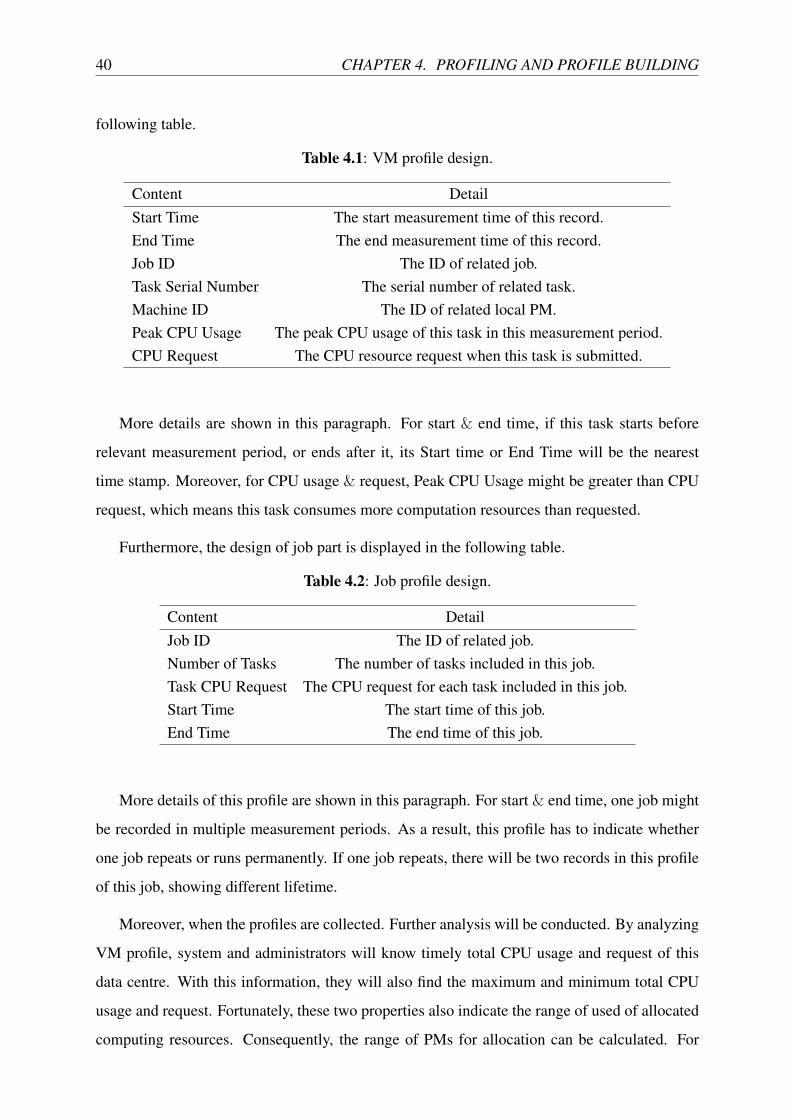
40 CHAPTER 4. PROFILING AND PROFILE BUILDING
following table.
Table 4.1: VM profile design.
Content DetailStart Time The start measurement time of this record.End Time The end measurement time of this record.Job ID The ID of related job.Task Serial Number The serial number of related task.Machine ID The ID of related local PM.Peak CPU Usage The peak CPU usage of this task in this measurement period.CPU Request The CPU resource request when this task is submitted.
More details are shown in this paragraph. For start & end time, if this task starts before
relevant measurement period, or ends after it, its Start time or End Time will be the nearest
time stamp. Moreover, for CPU usage & request, Peak CPU Usage might be greater than CPU
request, which means this task consumes more computation resources than requested.
Furthermore, the design of job part is displayed in the following table.
Table 4.2: Job profile design.
Content DetailJob ID The ID of related job.Number of Tasks The number of tasks included in this job.Task CPU Request The CPU request for each task included in this job.Start Time The start time of this job.End Time The end time of this job.
More details of this profile are shown in this paragraph. For start & end time, one job might
be recorded in multiple measurement periods. As a result, this profile has to indicate whether
one job repeats or runs permanently. If one job repeats, there will be two records in this profile
of this job, showing different lifetime.
Moreover, when the profiles are collected. Further analysis will be conducted. By analyzing
VM profile, system and administrators will know timely total CPU usage and request of this
data centre. With this information, they will also find the maximum and minimum total CPU
usage and request. Fortunately, these two properties also indicate the range of used of allocated
computing resources. Consequently, the range of PMs for allocation can be calculated. For
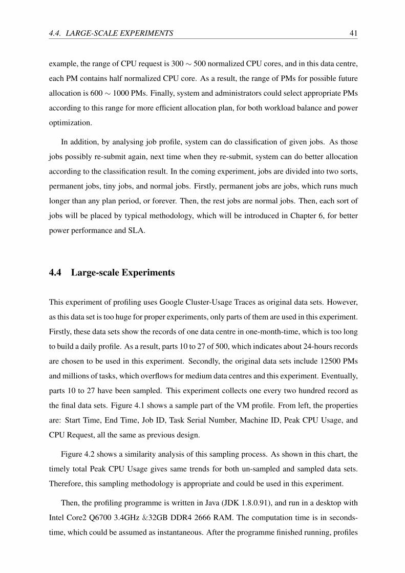
4.4. LARGE-SCALE EXPERIMENTS 41
example, the range of CPU request is 300∼ 500 normalized CPU cores, and in this data centre,
each PM contains half normalized CPU core. As a result, the range of PMs for possible future
allocation is 600 ∼ 1000 PMs. Finally, system and administrators could select appropriate PMs
according to this range for more efficient allocation plan, for both workload balance and power
optimization.
In addition, by analysing job profile, system can do classification of given jobs. As those
jobs possibly re-submit again, next time when they re-submit, system can do better allocation
according to the classification result. In the coming experiment, jobs are divided into two sorts,
permanent jobs, tiny jobs, and normal jobs. Firstly, permanent jobs are jobs, which runs much
longer than any plan period, or forever. Then, the rest jobs are normal jobs. Then, each sort of
jobs will be placed by typical methodology, which will be introduced in Chapter 6, for better
power performance and SLA.
4.4 Large-scale Experiments
This experiment of profiling uses Google Cluster-Usage Traces as original data sets. However,
as this data set is too huge for proper experiments, only parts of them are used in this experiment.
Firstly, these data sets show the records of one data centre in one-month-time, which is too long
to build a daily profile. As a result, parts 10 to 27 of 500, which indicates about 24-hours records
are chosen to be used in this experiment. Secondly, the original data sets include 12500 PMs
and millions of tasks, which overflows for medium data centres and this experiment. Eventually,
parts 10 to 27 have been sampled. This experiment collects one every two hundred record as
the final data sets. Figure 4.1 shows a sample part of the VM profile. From left, the properties
are: Start Time, End Time, Job ID, Task Serial Number, Machine ID, Peak CPU Usage, and
CPU Request, all the same as previous design.
Figure 4.2 shows a similarity analysis of this sampling process. As shown in this chart, the
timely total Peak CPU Usage gives same trends for both un-sampled and sampled data sets.
Therefore, this sampling methodology is appropriate and could be used in this experiment.
Then, the profiling programme is written in Java (JDK 1.8.0.91), and run in a desktop with
Intel Core2 Q6700 3.4GHz &32GB DDR4 2666 RAM. The computation time is in seconds-
time, which could be assumed as instantaneous. After the programme finished running, profiles

42 CHAPTER 4. PROFILING AND PROFILE BUILDING
Figure 4.1: Segment of VM profile sample.
Figure 4.2: Entire peak CPU usage in 24 hours.
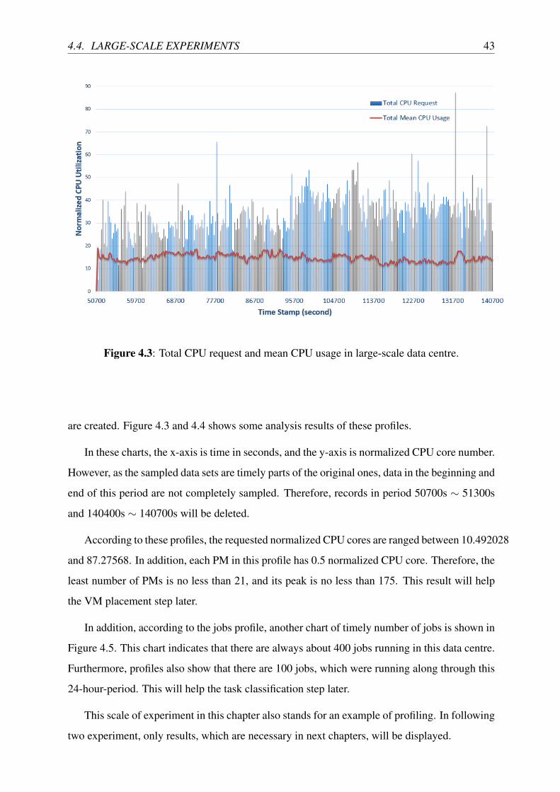
4.4. LARGE-SCALE EXPERIMENTS 43
Figure 4.3: Total CPU request and mean CPU usage in large-scale data centre.
are created. Figure 4.3 and 4.4 shows some analysis results of these profiles.
In these charts, the x-axis is time in seconds, and the y-axis is normalized CPU core number.
However, as the sampled data sets are timely parts of the original ones, data in the beginning and
end of this period are not completely sampled. Therefore, records in period 50700s ∼ 51300s
and 140400s ∼ 140700s will be deleted.
According to these profiles, the requested normalized CPU cores are ranged between 10.492028
and 87.27568. In addition, each PM in this profile has 0.5 normalized CPU core. Therefore, the
least number of PMs is no less than 21, and its peak is no less than 175. This result will help
the VM placement step later.
In addition, according to the jobs profile, another chart of timely number of jobs is shown in
Figure 4.5. This chart indicates that there are always about 400 jobs running in this data centre.
Furthermore, profiles also show that there are 100 jobs, which were running along through this
24-hour-period. This will help the task classification step later.
This scale of experiment in this chapter also stands for an example of profiling. In following
two experiment, only results, which are necessary in next chapters, will be displayed.
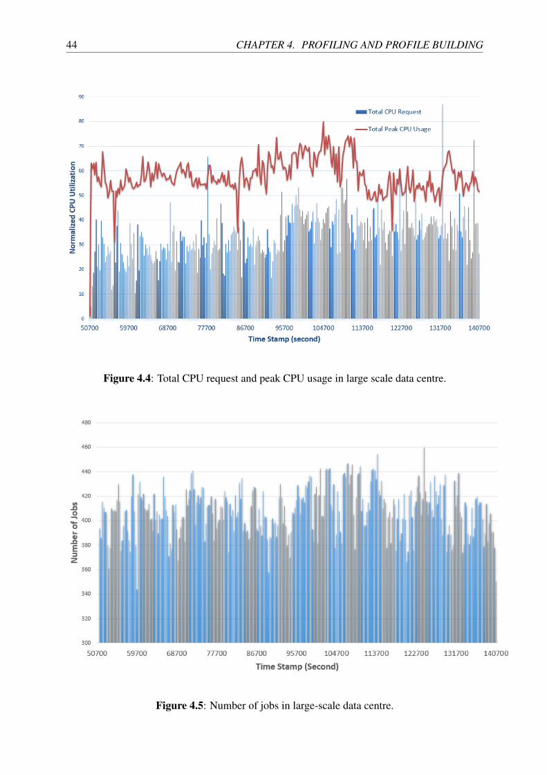
44 CHAPTER 4. PROFILING AND PROFILE BUILDING
Figure 4.4: Total CPU request and peak CPU usage in large scale data centre.
Figure 4.5: Number of jobs in large-scale data centre.
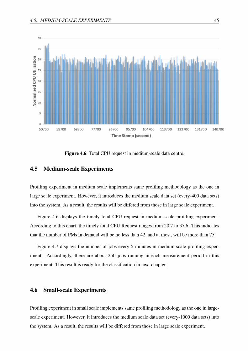
4.5. MEDIUM-SCALE EXPERIMENTS 45
Figure 4.6: Total CPU request in medium-scale data centre.
4.5 Medium-scale Experiments
Profiling experiment in medium scale implements same profiling methodology as the one in
large scale experiment. However, it introduces the medium scale data set (every-400 data sets)
into the system. As a result, the results will be differed from those in large scale experiment.
Figure 4.6 displays the timely total CPU request in medium scale profiling experiment.
According to this chart, the timely total CPU Request ranges from 20.7 to 37.6. This indicates
that the number of PMs in demand will be no less than 42, and at most, will be more than 75.
Figure 4.7 displays the number of jobs every 5 minutes in medium scale profiling exper-
iment. Accordingly, there are about 250 jobs running in each measurement period in this
experiment. This result is ready for the classification in next chapter.
4.6 Small-scale Experiments
Profiling experiment in small scale implements same profiling methodology as the one in large-
scale experiment. However, it introduces the medium scale data set (every-1000 data sets) into
the system. As a result, the results will be differed from those in large scale experiment.
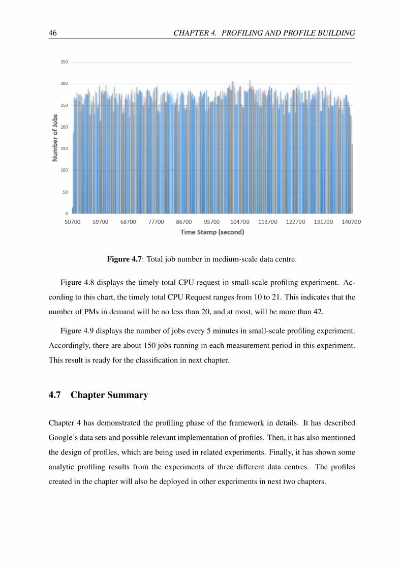
46 CHAPTER 4. PROFILING AND PROFILE BUILDING
Figure 4.7: Total job number in medium-scale data centre.
Figure 4.8 displays the timely total CPU request in small-scale profiling experiment. Ac-
cording to this chart, the timely total CPU Request ranges from 10 to 21. This indicates that the
number of PMs in demand will be no less than 20, and at most, will be more than 42.
Figure 4.9 displays the number of jobs every 5 minutes in small-scale profiling experiment.
Accordingly, there are about 150 jobs running in each measurement period in this experiment.
This result is ready for the classification in next chapter.
4.7 Chapter Summary
Chapter 4 has demonstrated the profiling phase of the framework in details. It has described
Google’s data sets and possible relevant implementation of profiles. Then, it has also mentioned
the design of profiles, which are being used in related experiments. Finally, it has shown some
analytic profiling results from the experiments of three different data centres. The profiles
created in the chapter will also be deployed in other experiments in next two chapters.
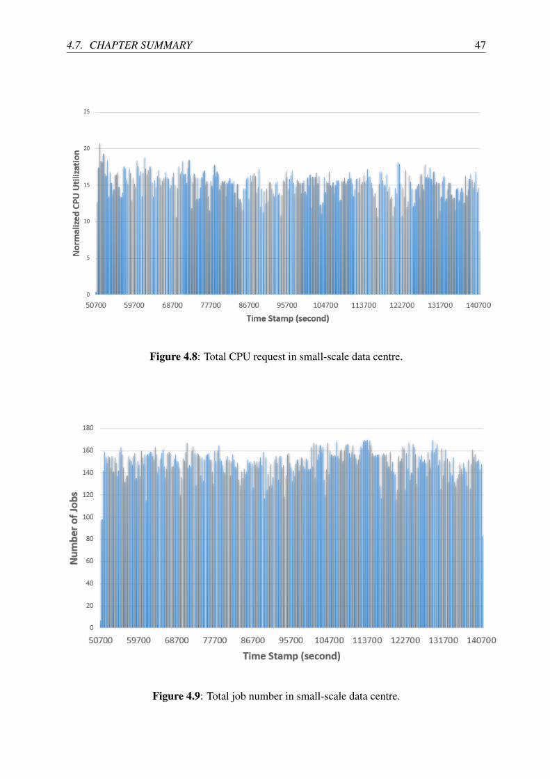
4.7. CHAPTER SUMMARY 47
Figure 4.8: Total CPU request in small-scale data centre.
Figure 4.9: Total job number in small-scale data centre.

48 CHAPTER 4. PROFILING AND PROFILE BUILDING
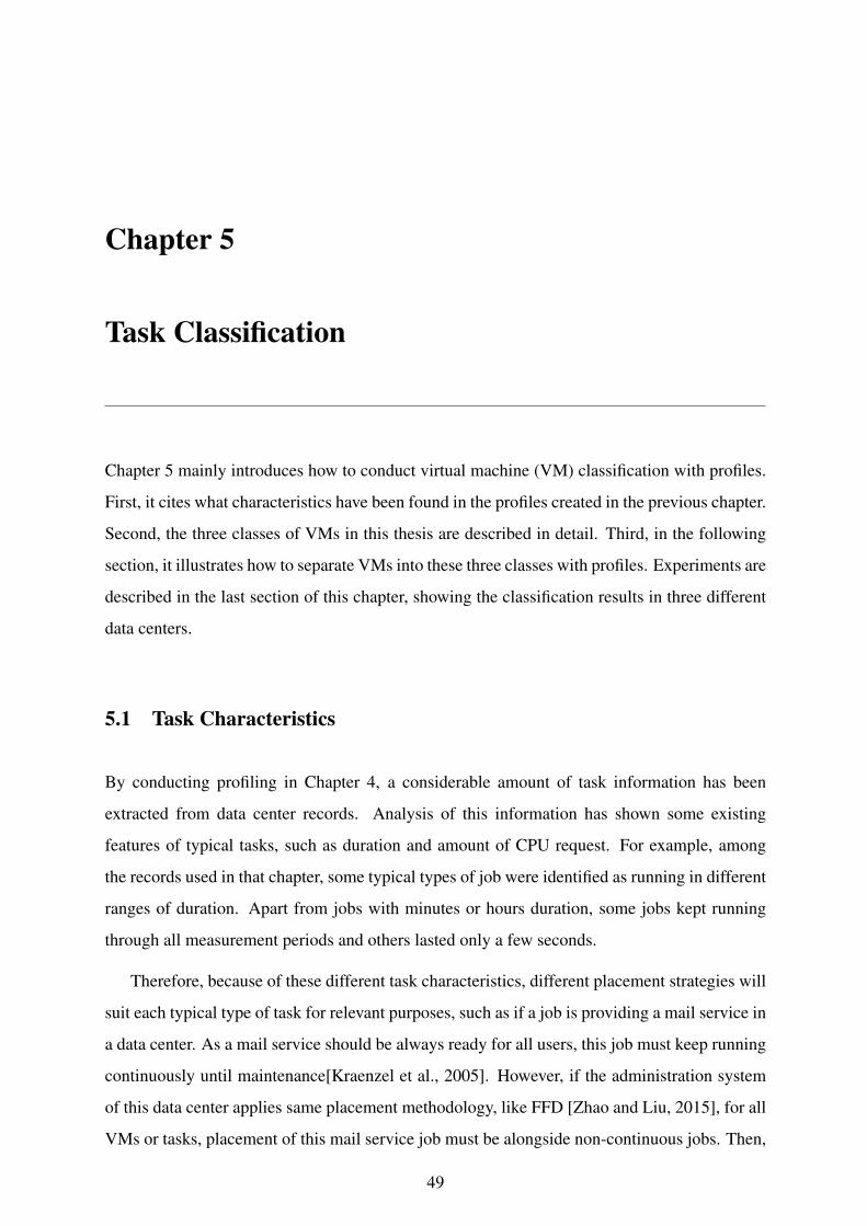
Chapter 5
Task Classification
Chapter 5 mainly introduces how to conduct virtual machine (VM) classification with profiles.
First, it cites what characteristics have been found in the profiles created in the previous chapter.
Second, the three classes of VMs in this thesis are described in detail. Third, in the following
section, it illustrates how to separate VMs into these three classes with profiles. Experiments are
described in the last section of this chapter, showing the classification results in three different
data centers.
5.1 Task Characteristics
By conducting profiling in Chapter 4, a considerable amount of task information has been
extracted from data center records. Analysis of this information has shown some existing
features of typical tasks, such as duration and amount of CPU request. For example, among
the records used in that chapter, some typical types of job were identified as running in different
ranges of duration. Apart from jobs with minutes or hours duration, some jobs kept running
through all measurement periods and others lasted only a few seconds.
Therefore, because of these different task characteristics, different placement strategies will
suit each typical type of task for relevant purposes, such as if a job is providing a mail service in
a data center. As a mail service should be always ready for all users, this job must keep running
continuously until maintenance[Kraenzel et al., 2005]. However, if the administration system
of this data center applies same placement methodology, like FFD [Zhao and Liu, 2015], for all
VMs or tasks, placement of this mail service job must be alongside non-continuous jobs. Then,
49
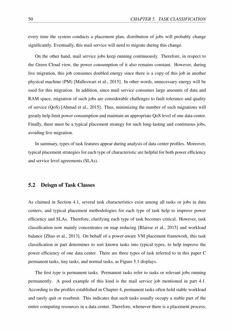
50 CHAPTER 5. TASK CLASSIFICATION
every time the system conducts a placement plan, distribution of jobs will probably change
significantly. Eventually, this mail service will need to migrate during this change.
On the other hand, mail service jobs keep running continuously. Therefore, in respect to
the Green Cloud view, the power consumption of it also remains constant. However, during
live migration, this job consumes doubled energy since there is a copy of this job in another
physical machine (PM) [Malleswari et al., 2015]. In other words, unnecessary energy will be
used for this migration. In addition, since mail service consumes large amounts of data and
RAM space, migration of such jobs are considerable challenges to fault tolerance and quality
of service (QoS) [Ahmad et al., 2015]. Thus, minimizing the number of such migrations will
greatly help limit power consumption and maintain an appropriate QoS level of one data center.
Finally, there must be a typical placement strategy for such long-lasting and continuous jobs,
avoiding live migration.
In summary, types of task features appear during analysis of data center profiles. Moreover,
typical placement strategies for each type of characteristic are helpful for both power efficiency
and service level agreements (SLAs).
5.2 Deisgn of Task Classes
As claimed in Section 4.1, several task characteristics exist among all tasks or jobs in data
centers, and typical placement methodologies for each type of task help to improve power
efficiency and SLAs. Therefore, clarifying each type of task becomes critical. However, task
classification now mainly concentrates on map reducing [Blaisse et al., 2015] and workload
balance [Zhao et al., 2013]. On behalf of a power-aware VM placement framework, this task
classification in part determines to sort known tasks into typical types, to help improve the
power efficiency of one data center. There are three types of task referred to in this paper C
permanent tasks, tiny tasks, and normal tasks, as Figure 5.1 displays.
The first type is permanent tasks. Permanent tasks refer to tasks or relevant jobs running
permanently. A good example of this kind is the mail service job mentioned in part 4.1.
According to the profiles established in Chapter 4, permanent tasks often hold stable workload
and rarely quit or resubmit. This indicates that such tasks usually occupy a stable part of the
entire computing resources in a data center. Therefore, whenever there is a placement process,
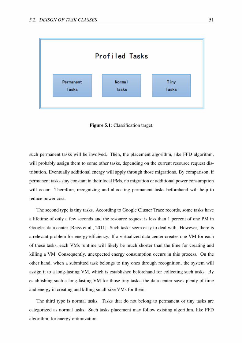
5.2. DEISGN OF TASK CLASSES 51
Figure 5.1: Classification target.
such permanent tasks will be involved. Then, the placement algorithm, like FFD algorithm,
will probably assign them to some other tasks, depending on the current resource request dis-
tribution. Eventually additional energy will apply through those migrations. By comparison, if
permanent tasks stay constant in their local PMs, no migration or additional power consumption
will occur. Therefore, recognizing and allocating permanent tasks beforehand will help to
reduce power cost.
The second type is tiny tasks. According to Google Cluster Trace records, some tasks have
a lifetime of only a few seconds and the resource request is less than 1 percent of one PM in
Googles data center [Reiss et al., 2011]. Such tasks seem easy to deal with. However, there is
a relevant problem for energy efficiency. If a virtualized data center creates one VM for each
of these tasks, each VMs runtime will likely be much shorter than the time for creating and
killing a VM. Consequently, unexpected energy consumption occurs in this process. On the
other hand, when a submitted task belongs to tiny ones through recognition, the system will
assign it to a long-lasting VM, which is established beforehand for collecting such tasks. By
establishing such a long-lasting VM for those tiny tasks, the data center saves plenty of time
and energy in creating and killing small-size VMs for them.
The third type is normal tasks. Tasks that do not belong to permanent or tiny tasks are
categorized as normal tasks. Such tasks placement may follow existing algorithm, like FFD
algorithm, for energy optimization.

52 CHAPTER 5. TASK CLASSIFICATION
5.3 Task Separation and Assignment Design
Task classification occurs alongside the creation of profiles, described in Chapter 4. For recog-
nizing the type of one task, its existing characteristics must also be recognised in this design.
This section introduced the methodologies of permanent and tiny tasks separation and their
allocation into suitable VMs.
The system will separate tasks into the three classes first. Whenever separation has finished,
the system will assign suitable VMs to those tasks regarding their requests and characteristics.
Figure 5.2 gives the work flow of the program in this experiment. The program collects all job
records from the given profile. Then it reads those records job by job. Whenever one job appears
in all measurement periods, the program will record it as a permanent job. This program runs
continuously until it has examined all jobs.
The pseudo code in algorithm 1 describes the separation and assignment algorithm to be
implemented.
Algorithm 1 Separation & assignment algorithm.1: procedure CLASSIFICATION
2: for all tasks do3: if Related job is in permanent jobList then4: task = permanent task5: else6: if task usage ≥ tiny threshold then7: task = normal task8: else9: task = tiny task
10: end if11: end if12: for all time slots do13: for all permanent and normal tasks do14: Assign separate VMs to each of them15: end for16: for all tiny tasks do17: if this task repeats regularly then18: Pack task19: Calculate package number20: end if21: end for22: end for23: end for24: end procedure
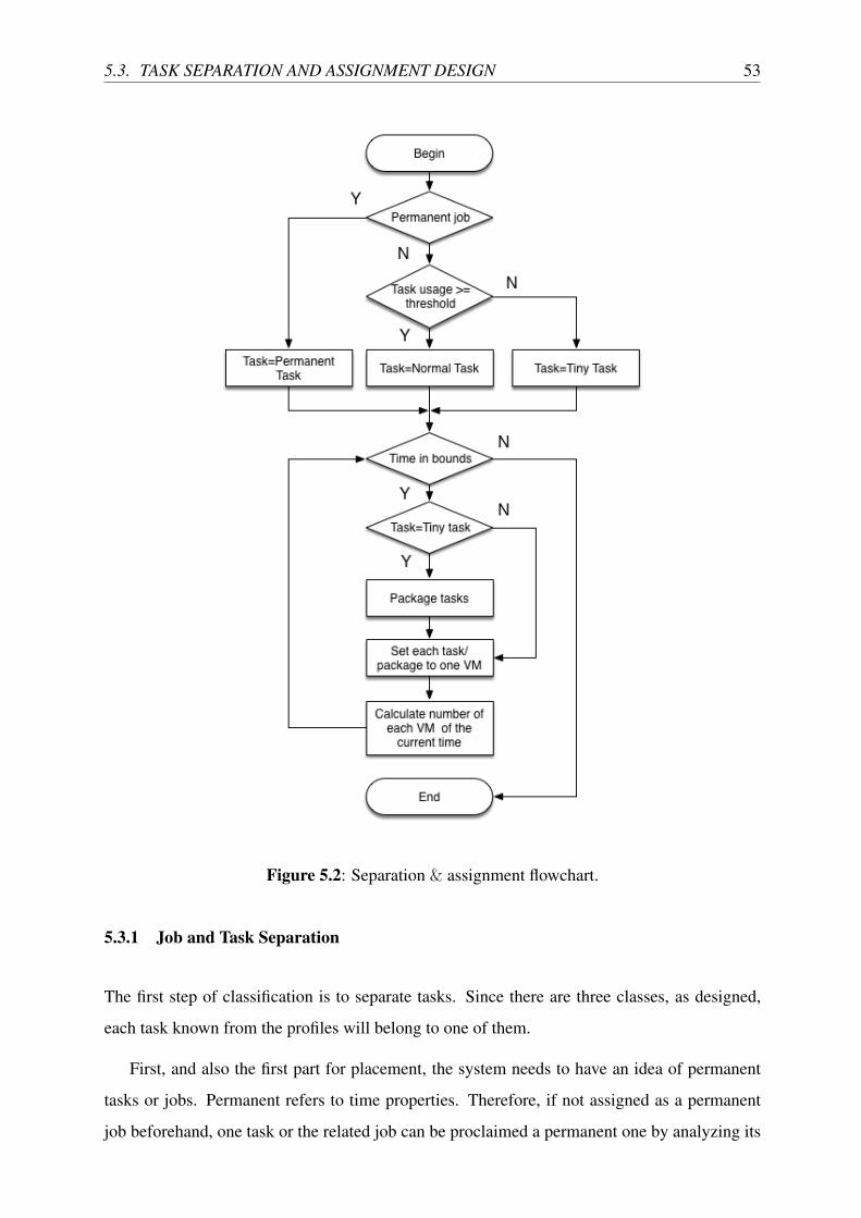
5.3. TASK SEPARATION AND ASSIGNMENT DESIGN 53
Figure 5.2: Separation & assignment flowchart.
5.3.1 Job and Task Separation
The first step of classification is to separate tasks. Since there are three classes, as designed,
each task known from the profiles will belong to one of them.
First, and also the first part for placement, the system needs to have an idea of permanent
tasks or jobs. Permanent refers to time properties. Therefore, if not assigned as a permanent
job beforehand, one task or the related job can be proclaimed a permanent one by analyzing its

54 CHAPTER 5. TASK CLASSIFICATION
lifetime. If this task or the related job have covered all existing measurement periods, the system
will sort this typical job as a permanent job. Consequently, typical placement methodology for
such permanents jobs will be introduced by the system.
The system separates permanent jobs and tasks by judging their lifetime. By mapping all
profiles created in Chapter 4, if a job includes tasks distributed among all measurement periods
in the profiles, this job will be judged as a permanent job. Finally, a permanent job list will be
formed, listing all permanent job IDs. Then all tasks belonging to those permanent jobs in the
list will be separated as permanent tasks.
Second, the system will separate tasks whose CPU requests are less than a given threshold
as tiny tasks. According to the profiles and task characteristics from Googles data sets, the
threshold in the following experiments are set as 0.015. In addition, such tasks usually have
a very tiny system utilization (such as 0.006425 or less) and a very short lifetime, which is
shorter than a normalized measurement period (300 seconds). As a result, such tasks will not
be assigned one VM for each. Otherwise small VMs are still too large for those tasks with
tiny utilization. These tiny tasks, which are in the same measurement periods, will probably be
packed into tiny VMs (with 0.015 capacity) to limit their system utilization.
5.3.2 Assignment of Tasks into VMs
The next step of classification is to assign suitable VMs to the tasks in typical classes. Previ-
ously, Vasudevan et al. [2017] has cited a special profile-based task (application) assignment
methodology. As the situation of relevant experiments in this thesis is not as complex as that in
Vasudevans paper, the system will assign tasks by FFD algorithm at most. Finally, in virtualized
data centers, all tasks must be allocated into suitable VMs before being placed.
Permanent and normal tasks are first assigned into separate VMs for each. As the perfor-
mance of VMs is fixed 3, each permanent or normal task will be assigned into a VM with best
suitable performance (normalized CPU capacity according to Googles data sets). For example,
a task with a CPU resource request of 0.125, will be assigned into a medium VM (with 0.15
normalized CPU capacity).
Next, tiny tasks will be packed and assigned into tiny VMs (with normalized 0.015 nor-
malized CPU capacity). According to profiles created in Chapter 4 3, tiny tasks often have a

5.4. RELATED EXPERIMENTS 55
very short lifetime, which is usually much less than a measurement period (300 seconds). In
addition, such tiny tasks often appear repeatedly and regularly. Therefore, these tiny tasks will
be packed and assigned into regular tiny VMs (with 0.015 normalized CPU capacity) rather
than separate VMs. However, not all tiny tasks can be packed in the experiments, as some of
them are not regular enough to join a package.
After all tasks have been assigned in relevant VMs, the framework will move into the next
phase of VM placement.
5.4 Related Experiments
As mentioned in the previous section, experiments in this chapter only include permanent
VMs classification. Tiny tasks classification experiments will go together with placement
experiments in the next chapter.
This experiment determines to verify whether the designed classification methodology works.
The classification program is also written in Java (JDK 1.8.0.91). In addition, the deployment
environment is a desktop with Intel Core2 Q6700 3.4GHz and 32GB DDR4 2666 RAM, in
Windows 10 Professional. Moreover, the data used in this experiment are profiles collected
in Chapter 4 experiments, including task usage records and related analysis tables. However,
as these profiles refer to sampled data sets, each job may not appear exactly the same in each
measurement period. As a result, this experiment sets an assumption that a job is continuous if
any of its tasks appear in continuous measurement periods.
5.4.1 Large-scale Experiments
Figure 5.3 displays the results of the large-scale experiment. As shown in this chart, there
are around 350 to 450 jobs in every measurement period (300 seconds). Among them, 100
jobs keep running continuously in all measurement periods. Therefore, these 100 jobs are the
permanent jobs for this data center. They will be given a separate placement methodology in
the next chapter.
Figure 5.4 and Figure 5.5 demonstrate the result of packing tiny tasks into tiny VMs in a
large-scale data center. The number of tiny task packages has the same trend as the number of
56 CHAPTER 5. TASK CLASSIFICATION
Figure 5.3: Large-scale classification result for permanent jobs.
tiny tasks. For example, in time stamp 54000, there are 307 tiny tasks, and 22 tiny task packages,
which will be assigned into 22 tiny VMs. In addition, in time stamp 104700, there are 1092 tiny
tasks, much more than those in time stamp 54000. As a result, 105 packages, through the same
trend, are created.
5.4.2 Medium-scale Experiments
Figure 5.6 displays the results of the medium-scale experiment. As shown in this chart, there
are around 220 to 300 jobs in every measurement period (300 seconds). Among them, 100
jobs keep running continuously in all measurement periods. Therefore, these 100 jobs are the
permanent jobs for this data center. They will also be given a separate placement methodology
in the chapter.
Figure 5.7 and Figure 5.8 demonstrate the result of packing tiny tasks into tiny VMs in a
medium-scale data center. The number of tiny task packages has the same trend as the number
of tiny tasks. For example, in time stamp 54000, there are 153 tiny tasks, and 11 tiny task
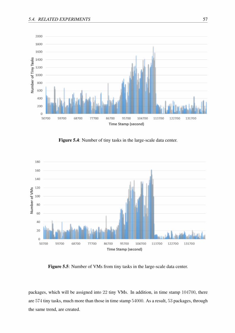
5.4. RELATED EXPERIMENTS 57
Figure 5.4: Number of tiny tasks in the large-scale data center.
Figure 5.5: Number of VMs from tiny tasks in the large-scale data center.
packages, which will be assigned into 22 tiny VMs. In addition, in time stamp 104700, there
are 574 tiny tasks, much more than those in time stamp 54000. As a result, 53 packages, through
the same trend, are created.
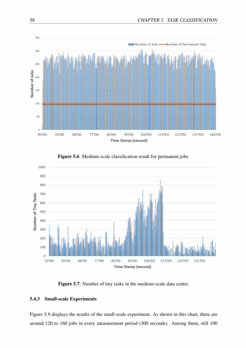
58 CHAPTER 5. TASK CLASSIFICATION
Figure 5.6: Medium-scale classification result for permanent jobs.
Figure 5.7: Number of tiny tasks in the medium-scale data center.
5.4.3 Small-scale Experiments
Figure 5.9 displays the results of the small-scale experiment. As shown in this chart, there are
around 120 to 160 jobs in every measurement period (300 seconds). Among them, still 100
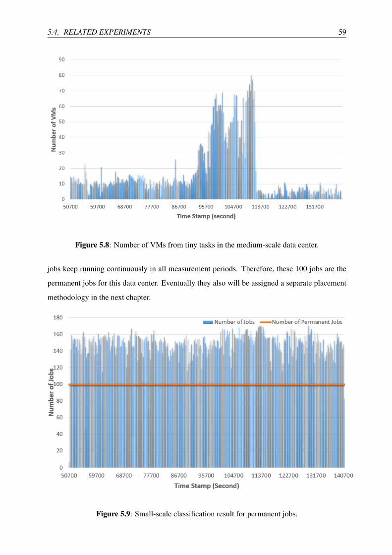
5.4. RELATED EXPERIMENTS 59
Figure 5.8: Number of VMs from tiny tasks in the medium-scale data center.
jobs keep running continuously in all measurement periods. Therefore, these 100 jobs are the
permanent jobs for this data center. Eventually they also will be assigned a separate placement
methodology in the next chapter.
Figure 5.9: Small-scale classification result for permanent jobs.

60 CHAPTER 5. TASK CLASSIFICATION
Figure 5.10 and Figure 5.11 demonstrate the result of packing tiny tasks into tiny VMs in
small-scale data center. The number of tiny task packages has the same trend as the number of
tiny tasks. For example, in time stamp 54000, there are 63 tiny tasks, and 5 tiny task packages,
which will be assigned into 22 tiny VMs. In addition, in time stamp 104700, there are 214 tiny
tasks, much more than those in time stamp 54000. As a result, 21 packages, also through the
same trend, are created.
Figure 5.10: Number of tiny tasks in the small-scale data center.
5.4.4 Discussions on Experiments
In summary, there are always 100 permanent running in all three scales of data centers. These
often refer to jobs like mail service and hyperviosrs, which are usually necessary in all data
centers. However, as the three data centers have different scales, those 100 permanent jobs
contain different numbers of tasks in each of them. The large-scale data center has more
permanent tasks than smaller ones.
5.5 Chapter Summary
Chapter 5 has discussed the second phase of the framework, task classification. It started with
typical characteristics of tasks, such as lifetime and resource requests. According to these
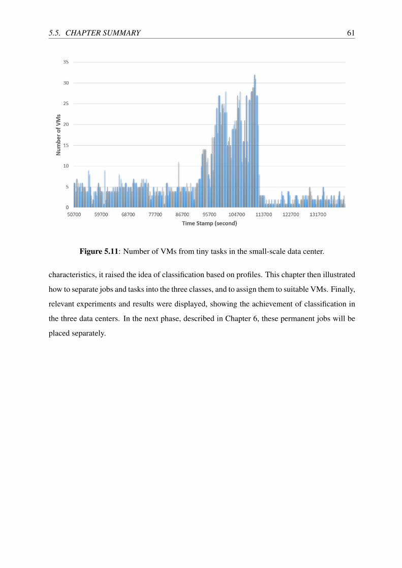
5.5. CHAPTER SUMMARY 61
Figure 5.11: Number of VMs from tiny tasks in the small-scale data center.
characteristics, it raised the idea of classification based on profiles. This chapter then illustrated
how to separate jobs and tasks into the three classes, and to assign them to suitable VMs. Finally,
relevant experiments and results were displayed, showing the achievement of classification in
the three data centers. In the next phase, described in Chapter 6, these permanent jobs will be
placed separately.

62 CHAPTER 5. TASK CLASSIFICATION
Chapter 6
Profile-based Virtual Machine Placement
In Chapters 4 and 5, virtual machine (VM) profiles were established and VM or jobs were
classified (permanent ones only). Finally, all necessary information is now ready to build
an energy-oriented VM placement plan for data centers. This plan will include all features
mentioned earlier, especially energy efficiency, guaranteed quality of service (QoS), and limited
migrations. By fulfilling this framework, a data center will be able to make better energy-
oriented VM placement plans through profiles and a private VM classification standard.
This chapter determines to clarify the VM placement methodology with advanced FFD
algorithm as the final part of the VM placement framework. A VM placement program will
be developed based on profiles and FFDalgorithm. This program will output a VM placement
plan for the data center administration system or administrators to place scheduled VMs for
better power efficiency. The proposed methodology is demonstrated through flow charts, and
simulation results are illustrated through numerical examples.
6.1 Profile-based VM Placement Scheme
This VM placement is the last part of the framework in this thesis. In Chapters 4 and 5, profiles
and VM classifications have already been well developed. According to the framework design
in Chapter 3 in Figure 3.2, this VM placement will inherit relevant results, profiles, and VM
classes to complete a VM placement plan to help save energy.
Through given profiles and related analysis results, the system will know VM-to-submit
63
64 CHAPTER 6. PROFILE-BASED VM PLACEMENT
schedules, as well as a timely computing resource request distribution. According to the VM-
to-submit schedules, the system is able to create the VM placement plan in advance, rather than
conducting real-time placement whenever a new VM submits. Moreover, with the distribution
of timely computing resource requests, both system and administrators will have a brief idea of
how many physical machines (PMs) should be included in each measurement period to suitably
satisfy the requests. As a result, the system will make better decisions over resource allocation
based on timely PM number, by limiting PM numbers to just fit the requests. Eventually, as the
number of PMs in use is directly related to power consumption, discussed in Chapter 3, limiting
PM numbers will help save energy in data centers.
In addition, a VM classification step in advance is also constructive for saving energy
in some non-directly related perspectives, such as long-term tasks allocation and potential
migration numbers.
First, allocating long-term VMs saves search area and energy. According to the analysis
results in Chapters 4 and 5, long-term, especially permanent jobs or tasks often require more
computing resources than those which last more shortly. Therefore, arranging these long-term
jobs or tasks, or relevant VMs, into PMs with better power efficiency will indirectly help to limit
power consumption. Moreover, placing long-term VMs in advance will help reduce migrations,
which usually consume more energy. By placing them in advance, the searching space of PMs
gets smaller accordingly, for the requests are smaller than all VMs requests. Therefore, those
long-term VMs will be assigned into fewer PMs, which also produces fewer possible PMs to be
switched off in the future. Thus, in a long-term view, less possible migration will occur since a
more limited number of PMs will be assigned.
Second, packing multiple regular tiny tasks into one VM saves total VM utilization [Va-
sudevan et al., 2017]. Compared with assigning separate VMs to each tiny task, packing those
tasks together will save possible utilization, which is the gap between task request and the size
of a VM. As a result, the total utilization of VMs will be restricted. Finally, fewer PMs will
probably be requisitioned and energy will be saved.
6.2. PROFILE-BASED VM PLACEMENT ARCHITECTURE 65
6.2 Profile-based VM Placement Architecture
Figure 6.1 displays the detailed architecture of VM placement in the new framework. First,
profiling and VM classification has classified VMs into three kinds C permanent jobs, normal
jobs and tasks, and tiny tasks. The first step of placement is to then assign VMs to those jobs
or tasks. Each task for permanent jobs and normal jobs and tasks will be assigned one VM,
which better fits the CPU request. However, multiple tiny tasks being packed into one VM
for their CPU requests is far less than the standard size of one VM. Next, permanent VMs
will be allocated first, and normal and tiny VMs will be allocated later, based on the results
of permanent VM allocation. Finally, the system will output a total VM placement plan to
administrators for reference.
6.3 FFD Algorithm in Profile-based VM Placement
The advanced FFD algorithm used in this thesis is based on the original FFD algorithm. Figure
6.2 gives the flow chart of this advanced FFD algorithm.
This framework determines to solve permanent, normal, and tiny tasks separately. First,
according to the classification result, each permanent task will be assigned into one VM, and be
well placed through the FFD algorithm. All other tasks will then be placed. The system keeps
allocating tasks one by one through the FFD algorithm until all ideal computing resources in
allocated PMs are available to the rest of the tasks. These remaining tasks will be treated as
tiny tasks automatically. At this stage, ideal VMs will be established in all allocated PMs, and
their sizes just fit the ideal computing resource. Tiny tasks, whose lifetime is often even shorter
than the duration of establishing and killing a VM, will be assigned to these VMs rather than
being assigned to one VM for each. After all tasks have been well placed, the system outputs a
placement plan and stops.
The following pseudo code gives a clearer idea of the FFD algorithm deployed in this
chapter.
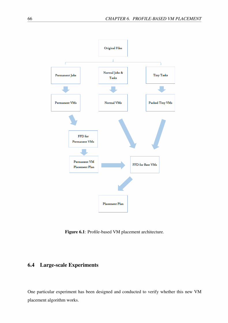
66 CHAPTER 6. PROFILE-BASED VM PLACEMENT
Figure 6.1: Profile-based VM placement architecture.
6.4 Large-scale Experiments
One particular experiment has been designed and conducted to verify whether this new VM
placement algorithm works.
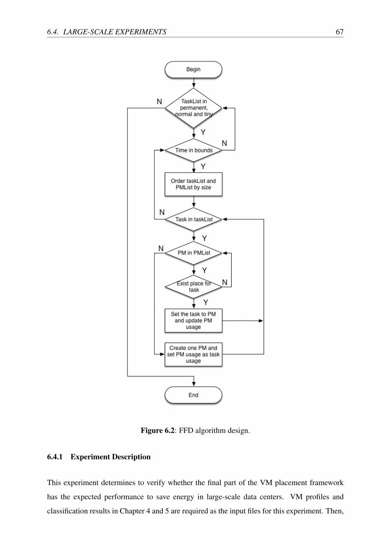
6.4. LARGE-SCALE EXPERIMENTS 67
Figure 6.2: FFD algorithm design.
6.4.1 Experiment Description
This experiment determines to verify whether the final part of the VM placement framework
has the expected performance to save energy in large-scale data centers. VM profiles and
classification results in Chapter 4 and 5 are required as the input files for this experiment. Then,
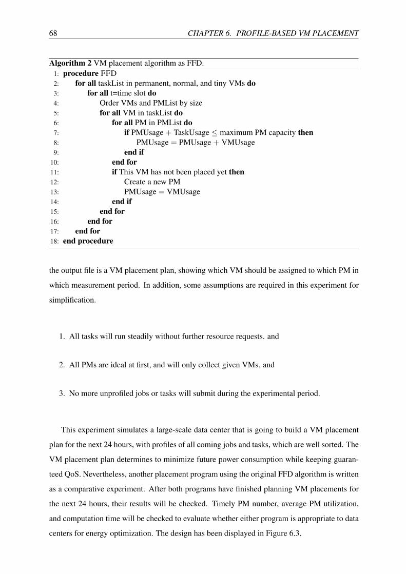
68 CHAPTER 6. PROFILE-BASED VM PLACEMENT
Algorithm 2 VM placement algorithm as FFD.1: procedure FFD2: for all taskList in permanent, normal, and tiny VMs do3: for all t=time slot do4: Order VMs and PMList by size5: for all VM in taskList do6: for all PM in PMList do7: if PMUsage + TaskUsage ≤ maximum PM capacity then8: PMUsage = PMUsage + VMUsage9: end if
10: end for11: if This VM has not been placed yet then12: Create a new PM13: PMUsage = VMUsage14: end if15: end for16: end for17: end for18: end procedure
the output file is a VM placement plan, showing which VM should be assigned to which PM in
which measurement period. In addition, some assumptions are required in this experiment for
simplification.
1. All tasks will run steadily without further resource requests. and
2. All PMs are ideal at first, and will only collect given VMs. and
3. No more unprofiled jobs or tasks will submit during the experimental period.
This experiment simulates a large-scale data center that is going to build a VM placement
plan for the next 24 hours, with profiles of all coming jobs and tasks, which are well sorted. The
VM placement plan determines to minimize future power consumption while keeping guaran-
teed QoS. Nevertheless, another placement program using the original FFD algorithm is written
as a comparative experiment. After both programs have finished planning VM placements for
the next 24 hours, their results will be checked. Timely PM number, average PM utilization,
and computation time will be checked to evaluate whether either program is appropriate to data
centers for energy optimization. The design has been displayed in Figure 6.3.
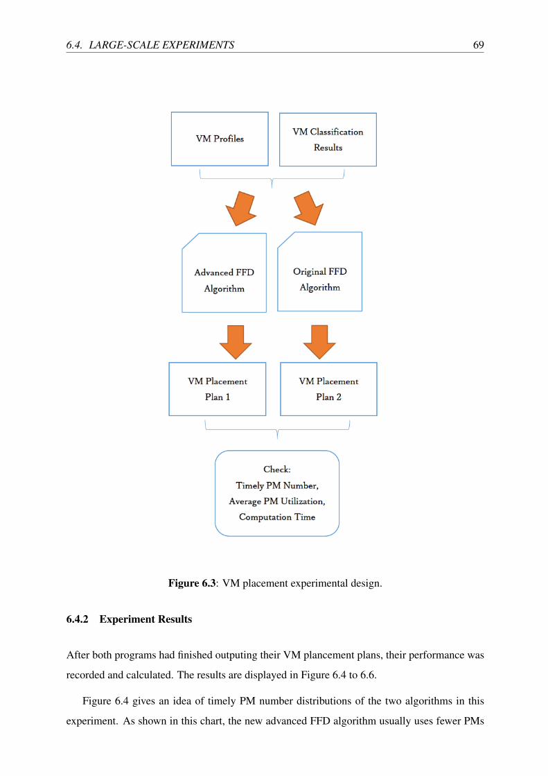
6.4. LARGE-SCALE EXPERIMENTS 69
Figure 6.3: VM placement experimental design.
6.4.2 Experiment Results
After both programs had finished outputing their VM plancement plans, their performance was
recorded and calculated. The results are displayed in Figure 6.4 to 6.6.
Figure 6.4 gives an idea of timely PM number distributions of the two algorithms in this
experiment. As shown in this chart, the new advanced FFD algorithm usually uses fewer PMs

70 CHAPTER 6. PROFILE-BASED VM PLACEMENT
than the original FFD algorithm in many measurement periods. This also means that the new
FFD algorithm will probably be more energy efficient.
Figure 6.4: Large-scale VM placement experiment result: timely PM quantity.
Figure 6.5 demonstrates a clearer view of the performance gap between these two algo-
rithms. In this chart, the Y-axis is the value of the PM number gap in each measurement period.
If the value is above zero, the new advanced FFD algorithm used more PMs than the original
FFD algorithm. If the value is below zero, the new advanced FFD algorithm used fewer PMs
than the original FFD algorithm. In addition, the value itself indicates how many PMs differed
between the two algorithms used in relevant time intervals. It is clear in this chart that 1 or
more, at most 37, PMs are usually saved by the new advanced FFD algorithm. Typically, during
time stamp from 92700 to 111600, the new framework saves far more PMs than the original
FFD. This is due to the fact that the number of tiny tasks explodes during this period, and the
new framework packs them rather than assigns separate VMs to each of them. Therefore, the
total utilization for VMs is limited, and PMs are saved as well. In addition, the PMs saved in
this experiment are all PMs with the least power efficiency.
Figure 6.6 displays the timely average PM utilization in all measurement periods. As
6.5. MEDIUM-SCALE EXPERIMENTS 71
Figure 6.5: Large-scale VM placement experiment result: PM number overlap.
mentioned in Chapter 3, greater utilization is often related to better energy efficiency. In this
chart, the average utilization of the new advanced FFD algorithm was often greater than the
original FFD algorithm. The result indicates that the energy efficiency of the new advanced
FFD algorithm was often better than the original. In other words, the new algorithm was able
to include more computation workload than the original when given the same power supply.
6.5 Medium-scale Experiments
Similar to the large-scale experiment, the data sets and previous results related to medium-scale
data center are used in the following experiment.
6.5.1 Experiment Description
This experiment determines to verify whether the final part of the VM placement framework
has the expected performance in saving energy in medium-scale data centers. All settings are
similar to those of the large-scale experiment, except the input data sets.
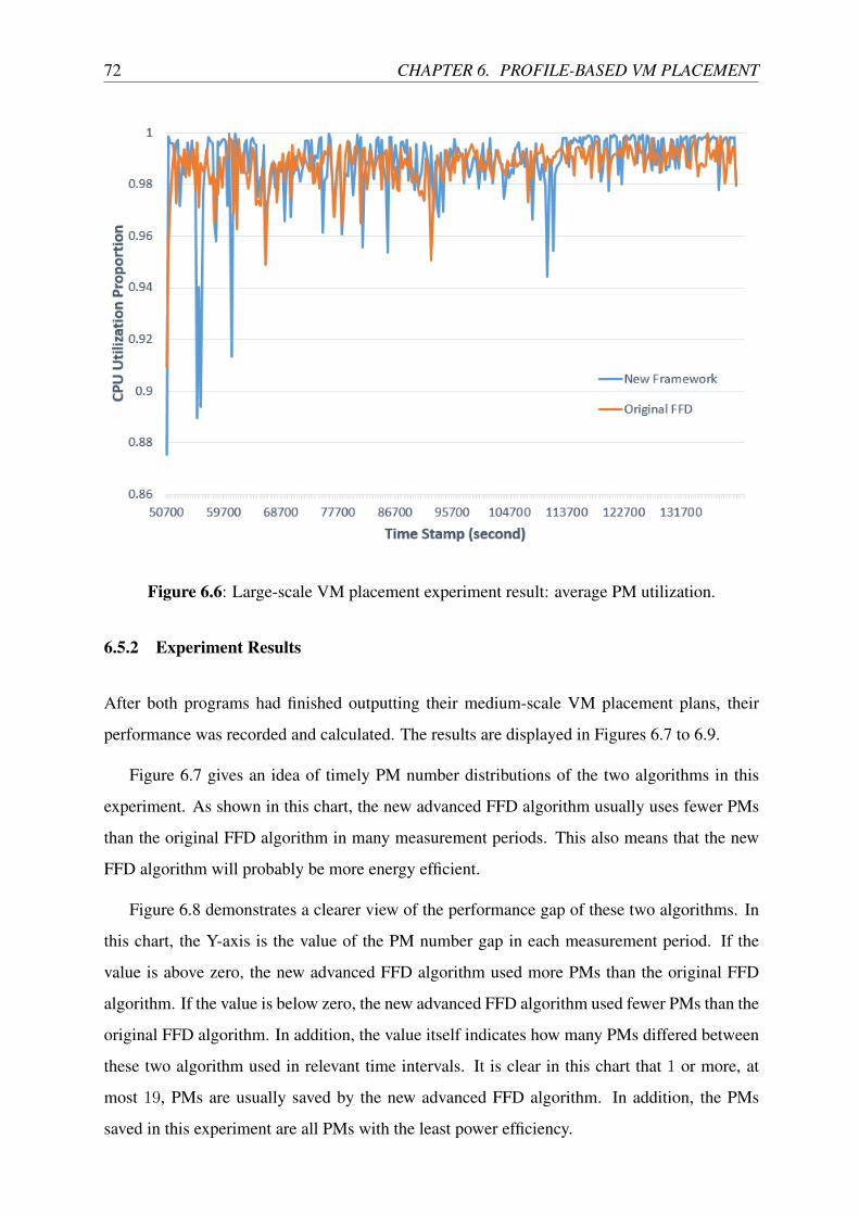
72 CHAPTER 6. PROFILE-BASED VM PLACEMENT
Figure 6.6: Large-scale VM placement experiment result: average PM utilization.
6.5.2 Experiment Results
After both programs had finished outputting their medium-scale VM placement plans, their
performance was recorded and calculated. The results are displayed in Figures 6.7 to 6.9.
Figure 6.7 gives an idea of timely PM number distributions of the two algorithms in this
experiment. As shown in this chart, the new advanced FFD algorithm usually uses fewer PMs
than the original FFD algorithm in many measurement periods. This also means that the new
FFD algorithm will probably be more energy efficient.
Figure 6.8 demonstrates a clearer view of the performance gap of these two algorithms. In
this chart, the Y-axis is the value of the PM number gap in each measurement period. If the
value is above zero, the new advanced FFD algorithm used more PMs than the original FFD
algorithm. If the value is below zero, the new advanced FFD algorithm used fewer PMs than the
original FFD algorithm. In addition, the value itself indicates how many PMs differed between
these two algorithm used in relevant time intervals. It is clear in this chart that 1 or more, at
most 19, PMs are usually saved by the new advanced FFD algorithm. In addition, the PMs
saved in this experiment are all PMs with the least power efficiency.
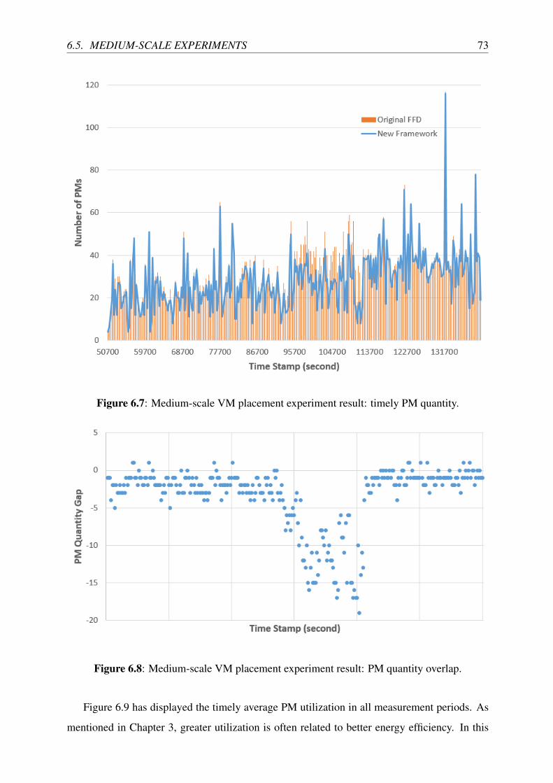
6.5. MEDIUM-SCALE EXPERIMENTS 73
Figure 6.7: Medium-scale VM placement experiment result: timely PM quantity.
Figure 6.8: Medium-scale VM placement experiment result: PM quantity overlap.
Figure 6.9 has displayed the timely average PM utilization in all measurement periods. As
mentioned in Chapter 3, greater utilization is often related to better energy efficiency. In this

74 CHAPTER 6. PROFILE-BASED VM PLACEMENT
chart, the average utilization of the new advanced FFD algorithm was often greater than the
original FFD algorithm. This result indicates that the energy efficiency of the new advanced
FFD algorithm was often better than the original. In other words, the new algorithm was able
to include more computation workload than the original when given the same power supply.
Figure 6.9: Medium-scale VM placement experiment Result: average PM utilization.
6.6 Small-scale Experiments
Similar to large- and medium-scale experiments, the data sets and previous results related to
small-scale data center are used in the following experiment.
6.6.1 Experiment Description
This experiment determines to verify whether the final part of the VM placement framework has
the expected performance in saving energy in small-scale data centers. All settings are similar
to those used in the large- and medium-scale experiments, except the input data sets.

6.6. SMALL-SCALE EXPERIMENTS 75
6.6.2 Experiment Results
After both programs had finished outputting their small-scale VM placement plans, their per-
formance was recorded and calculated. The results are displayed in Figures 6.10 to 6.12.
Figure 6.10 gives an idea of timely PM number distributions of the two algorithms in this
experiment. As shown in this chart, the new advanced FFD algorithm usually uses fewer PMs
than the original FFD algorithm in many measurement periods. This also means that the new
FFD algorithm will probably be more energy efficient.
Figure 6.10: Small-scale VM placement experiment result: timely PM quantity.
Figure 6.11 demonstrates a clearer view of the performance gap between these two algo-
rithms. In this chart, the Y-axis is the value of the PM number gap in each measurement period.
If the value is above zero, the new advanced FFD algorithm used more PMs than the original
FFD algorithm. If the value is below zero, the new advanced FFD algorithm used fewer PMs
than the original FFD algorithm. In addition, the value itself indicates how many PMs differeed
between these two algorithm used in relevant time intervals. It is clear in this chart that 1 or
more, at most 8, PMs are usually saved by the new advanced FFD algorithm. In addition, the
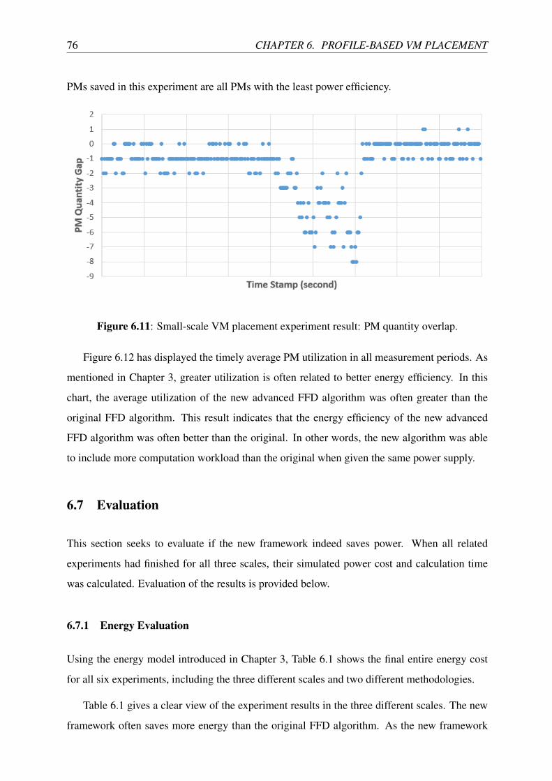
76 CHAPTER 6. PROFILE-BASED VM PLACEMENT
PMs saved in this experiment are all PMs with the least power efficiency.
Figure 6.11: Small-scale VM placement experiment result: PM quantity overlap.
Figure 6.12 has displayed the timely average PM utilization in all measurement periods. As
mentioned in Chapter 3, greater utilization is often related to better energy efficiency. In this
chart, the average utilization of the new advanced FFD algorithm was often greater than the
original FFD algorithm. This result indicates that the energy efficiency of the new advanced
FFD algorithm was often better than the original. In other words, the new algorithm was able
to include more computation workload than the original when given the same power supply.
6.7 Evaluation
This section seeks to evaluate if the new framework indeed saves power. When all related
experiments had finished for all three scales, their simulated power cost and calculation time
was calculated. Evaluation of the results is provided below.
6.7.1 Energy Evaluation
Using the energy model introduced in Chapter 3, Table 6.1 shows the final entire energy cost
for all six experiments, including the three different scales and two different methodologies.
Table 6.1 gives a clear view of the experiment results in the three different scales. The new
framework often saves more energy than the original FFD algorithm. As the new framework

6.7. EVALUATION 77
Figure 6.12: Small-scale VM placement experiment result: average PM utilization.
Table 6.1: Entire energy cost for all six experiments. The given numbers are the simulatedenergy cost in each data center over about 24 hours, expressed in joules. A percentage gapshows the percentage of energy the new framework saves.
New Framework Original FFD Algorithm Percentage GapLarge-scale 1.391 ∗ 109 1.585 ∗ 109 12.240%
Medium-Scale 6.011 ∗ 108 6.833 ∗ 108 12.030%
Small-Scale 3.632 ∗ 108 3.947 ∗ 108 7.981%
still deploys the FFD algorithm for each placement step (tasks to VMs, VMs to PMs), the energy
saved by the new framework is due to the classification of tasks and advanced assignment of
those classified tasks to VMs. For example, in the new framework, tiny tasks are packed into
fewer VMs rather than allocated to separated VMs each. As VMs are in fixed sizes, this typical
assignment for tiny tasks has saved hundreds of VMs, which may represent a high level of
utilization. By reducing the number of VMs and utilization, fewer PMs will be used to collect
those VMs (tasks). Therefore, energy is saved.
The new framework has saved about 10 percent more energy than the original FFD algo-
rithm. This is a considerable amount of energy, and cost. For example, if one data center spends
4, 000, 000 dollars on servers power supply with the original FFD algorithm, a 400, 000-dollar
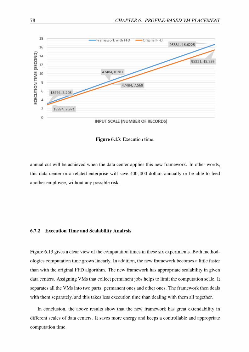
78 CHAPTER 6. PROFILE-BASED VM PLACEMENT
Figure 6.13: Execution time.
annual cut will be achieved when the data center applies this new framework. In other words,
this data center or a related enterprise will save 400, 000 dollars annually or be able to feed
another employee, without any possible risk.
6.7.2 Execution Time and Scalability Analysis
Figure 6.13 gives a clear view of the computation times in these six experiments. Both method-
ologies computation time grows linearly. In addition, the new framework becomes a little faster
than with the original FFD algorithm. The new framework has appropriate scalability in given
data centers. Assigning VMs that collect permanent jobs helps to limit the computation scale. It
separates all the VMs into two parts: permanent ones and other ones. The framework then deals
with them separately, and this takes less execution time than dealing with them all together.
In conclusion, the above results show that the new framework has great extendability in
different scales of data centers. It saves more energy and keeps a controllable and appropriate
computation time.

6.8. CHAPTER SUMMARY 79
6.8 Chapter Summary
Chapter 6 has addressed the final phase of the framework, VM placement. By implementing
profiles and classification results, the framework is able to conduct resource allocation for better
energy efficiency than the original FFD algorithm. The experiments and relevant results also
prove that the new VM placement framework saved as much as12 percent power with little
execution time extension.

80 CHAPTER 6. PROFILE-BASED VM PLACEMENT
Chapter 7
Conclusions and Recommendations
7.1 Summary of the Research
This thesis has introduced a new energy-aware virtual machine (VM) placement framework
that implements profiling, classification, and FFD algorithm. This new framework helps data
centers of all different scales save energy through better resource allocation methodology, while
guaranteeing Quality of Service (QoS).
This thesis has examined the problem of skyrocketing power consumption in data centers,
discussed industrial methodologies to solve it, and checked recent research explorations in this
field. It has combined all advantages and disadvantages of recent methodologies to form this
new framework. Moreover, this paper has formulated the energy problem through equations
and established a power model of CPUs for accurate evaluation.
The new VM placement framework includes three parts: profiling, VM classification, and
placement. The paper has used three chapters to describe each part in detail. In addition,
relevant experiments and results have been provided in each chapter. The results have shown
that this new framework was able to save about 10 percent or more energy than the existing
FFD algorithm.
This new power-aware VM placement framework will make enterprises more comfortable
when establishing a new data center. It will help such data centers complete better cost control
and improve QoS.
81
82 CHAPTER 7. CONCLUSIONS AND RECOMMENDATIONS
7.2 Recommendations and Future Work
The new power-aware VM placement framework now better fits data centers with adequate
profiles, such as the private data centers of enterprises. Hence, it is recommended that this
framework is implemented in private data centers, such as the internal data centers of banks,
grocery groups, and governmental agencies.
In future research, some parts of this framework can be improved. First, the algorithm can
be improved. This framework has used FFD algorithm for VM placement. However, FFD
algorithm is now not as good as other algorithms, such as BFD or GA, in power efficiency.
In future research stages, the algorithm should be changed to meet the demands of both better
energy efficiency and shorter execution time.
Second, the profile-based strategies and framework can be further improved for more com-
plicated scenarios. The profiles currently include only CPU information. In future research,
the profiles should include more information about memory, disk, and network, to meet more
complicated situations in different data centers. This will allow more detailed classification of
tasks, and thus more precise description of various profiles.
This new profile-based VM placement framework for energy optimization will significantly
contribute to the energy cost management of virtualized data centers, limit worldwide energy
resource consumption, and relieve the greenhouse effect for both recent and future generations.
Literature Cited
Ahmad, R. W., Gani, A., Hamid, S. H. A., Shiraz, M., Xia, F., and Madani, S. A. (2015). Virtual
machine migration in cloud data centers: a review, taxonomy, and open research issues. The
Journal of Supercomputing, 71(7):2473–2515.
Amazon-Web-Services (2016). Amazon ec2 product details. https://aws.amazon.com/
ec2/details/.
Beloglazov, A., Buyya, R., Lee, Y. C., Zomaya, A., et al. (2011). A taxonomy and survey
of energy-efficient data centers and cloud computing systems. Advances in computers,
82(2):47–111.
Blaisse, A. P., Wagner, Z. A., and Wu, J. (2015). Selection of virtual machines based on
classification of mapreduce jobs. In 2015 IEEE 35th International Conference on Distributed
Computing Systems Workshops, pages 82–86. IEEE.
Breg, F. and Polychronopoulos, C. D. (2001). Java virtual machine support for object
serialization. In Proceedings of the 2001 joint ACM-ISCOPE conference on Java Grande,
pages 173–180. ACM.
Buyya, R., Beloglazov, A., and Abawajy, J. (2010). Energy-efficient management of data center
resources for cloud computing: A vision, architectural elements, and open challenges. arXiv
preprint arXiv:1006.0308.
Dai, X., Wang, J. M., and Bensaou, B. (2016). Energy-efficient virtual machines scheduling in
multi-tenant data centers.
Dickson, P. R. (2015). The adoption of customer service improvement practices. Marketing
Letters, 26(1):1–15.
Douglis, F. and Krieger, O. (2013). Virtualization. IEEE Internet Computing, 17(2):6–9.
83
84 LITERATURE CITED
Graubner, P., Schmidt, M., and Freisleben, B. (2013). Energy-efficient virtual machine
consolidation. It Professional, 15(2):28–34.
Kajamoideen, M. R. and Sivaraman, A. (2014). VMware ESXi Cookbook. Packt Publishing
Ltd.
Kraenzel, C. J., Immerman, J. D., Mills, W. A., Nowacki, M. A., and Lu, J. J. (2005). System
and method for managing concurrent scheduled or on-demand replication of subscriptions.
US Patent 6,845,383.
Lama, P. (2007). Autonomic performance and power control in virtualized datacenters.
Liu, Z., Liu, I., Low, S., and Wierman, A. (2014). Pricing data center demand response. ACM
SIGMETRICS Performance Evaluation Review, 42(1):111–123.
Liu, Z., Xiang, Y., and Qu, X. (2015). Towards optimal cpu frequency and different workload
for multi-objective vm allocation. In 2015 12th Annual IEEE Consumer Communications
and Networking Conference (CCNC), pages 367–372. IEEE.
Luo, J., Rao, L., and Liu, X. (2014). Temporal load balancing with service delay guarantees for
data center energy cost optimization. IEEE Transactions on Parallel and Distributed Systems,
25(3):775–784.
Malleswari, T. N., Vadivu, G., and Malathi, D. (2015). Live virtual machine migration
techniquesa technical survey. In Intelligent Computing, Communication and Devices, pages
303–319. Springer.
Matlis, J. (2006). Virtual machines.
McClurg, J., Zhang, Y., Wheeler, J., and Pilawa-Podgurski, R. (2013). Re-thinking data center
power delivery: Regulating series-connected voltage domains in software. In Power and
Energy Conference at Illinois (PECI), 2013 IEEE, pages 147–154. IEEE.
Minarolli, D. and Freisleben, B. (2011). Utility-based resource allocation for virtual machines
in cloud computing. In Computers and Communications (ISCC), 2011 IEEE Symposium on,
pages 410–417. IEEE.
Mishra, M., Das, A., Kulkarni, P., and Sahoo, A. (2012). Dynamic resource management using
virtual machine migrations. IEEE Communications Magazine, 50(9):34–40.
LITERATURE CITED 85
Mobius, C., Dargie, W., and Schill, A. (2014). Power consumption estimation models for
processors, virtual machines, and servers. IEEE Transactions on Parallel and Distributed
Systems, 25(6):1600–1614.
Monteiro, R. C., Dantas, M., and y Rodriguez, M. V. R. (2014). Green cloud computing: An
experimental validation. In Journal of Physics: Conference Series, volume 540, page 012005.
IOP Publishing.
Moore, G. E. (2006). Cramming more components onto integrated circuits, reprinted from
electronics, volume 38, number 8, april 19, 1965, pp. 114 ff. IEEE Solid-State Circuits
Newsletter, 3(20):33–35.
Reiss, C., Tumanov, A., Ganger, G. R., Katz, R. H., and Kozuch, M. A. (2012). Heterogeneity
and dynamicity of clouds at scale: Google trace analysis. In Proceedings of the Third ACM
Symposium on Cloud Computing, page 7. ACM.
Reiss, C., Wilkes, J., and Hellerstein, J. L. (2011). Google cluster-usage traces: format+
schema. Google Inc., White Paper, pages 1–14.
Sato, K., Samejima, M., and Komoda, N. (2013). Dynamic optimization of virtual machine
placement by resource usage prediction. In 2013 11th IEEE International Conference on
Industrial Informatics (INDIN), pages 86–91. IEEE.
Thraves, C. and Wang, L. (2014). Power-efficient assignment of virtual machines to physical
machines. In Adaptive Resource Management and Scheduling for Cloud Computing: First
International Workshop, ARMS-CC 2014, held in Conjunction with ACM Symposium on
Principles of Distributed Computing, PODC 2014, Paris, France, July 15, 2014, Revised
Selected Papers, volume 8907, page 71. Springer.
Vasudevan, M., Tian, Y.-C., Tang, M., and Kozan, E. (2017). Profile-based application
assignment for greener and more energy-efficient data centers. Future Generation Computer
Systems, 67:94–108.
Versick, D., Waßmann, I., and Tavangarian, D. (2013). Power consumption estimation of cpu
and peripheral components in virtual machines. ACM SIGAPP Applied Computing Review,
13(3):17–25.
86 LITERATURE CITED
Wang, X., Wang, X., Xing, G., Chen, J., Lin, C.-X., and Chen, Y. (2013). Intelligent sensor
placement for hot server detection in data centers. IEEE Transactions on Parallel and
Distributed Systems, 24(8):1577–1588.
Williams, D. E. (2007). Virtualization with Xen (tm): Including XenEnterprise, XenServer, and
XenExpress. Syngress.
Yu, L., Jiang, T., Cao, Y., and Qi, Q. (2015). Joint workload and battery scheduling with
heterogeneous service delay guaranteesfor data center energy cost minimization. IEEE
Transactions on Parallel and Distributed Systems, 26(7):1937–1947.
Zhang, S., Yang, J., Shi, Y., Wu, X., and Ran, Y. (2015). Dynamic energy storage control for
reducing electricity cost in data centers. Mathematical Problems in Engineering, 2015.
Zhao, C. and Liu, J. (2015). A virtual machine dynamic consolidation algorithm based dynamic
complementation and ffd algorithm. In Communication Systems and Network Technologies
(CSNT), 2015 Fifth International Conference on, pages 333–338. IEEE.
Zhao, X., Yin, J., Chen, Z., and He, S. (2013). Workload classification model for specializing
virtual machine operating system. In 2013 IEEE Sixth International Conference on Cloud
Computing, pages 343–350. IEEE.
Zhou, X. and Jiang, C.-J. (2014). Autonomic performance and power control on virtualized
servers: Survey, practices, and trends. Journal of Computer Science and Technology,
29(4):631–645.