NISTIR 6806

Project-Oriented Life-Cycle CostingWorkshop for Energy Conservationin BuildingsSieglinde K. FullerAmy S. RushingGene M. Meyer

U.S. DEPARTMENT OF COMMERCETechnology AdministrationNational Institute of Standards andTechnology

Prepared for:United States Department of EnergyFederal Energy Management Program

NISTIR 6806

Project-Oriented Life-Cycle CostingWorkshop For Energy Conservationin BuildingsSieglinde K. FullerAmy S. RushingOffice of Applied Economics

Gene M. MeyerKansas State University

September 2001 Sponsored by:Building and Fire Research Laboratory The Federal Energy Management ProgramNational Institute of Standards and Technology U.S. Department of EnergyGaithersburg, MD 20899 Washington, DC 20585

U.S. Department of CommerceDonald L. Evans, Secretary

National Institute of Standards and TechnologyKaren H. Brown, Acting Director

Disclaimer

Use of Non-Metric Units in NIST Internal Report No. 6806

The policy of the National Institute of Standards and Technology is to use metric units of measurement inall its publications. NISTIR 6806 is intended for a workshop audience that deals with energy projects forbuildings and building systems. In construction-related industries in North America certain non-metricunits are so widely used instead of metric units that it is more practical and less confusing to include inthis workbook only measurement values for customary units.

iii

Table of Contents

Table of Contents........................................................................................................................... iii

Preface..............................................................................................................................................v

Acknowledgements...................................................................................................................... viii

Instructor Profiles .......................................................................................................................... ix

Workshop Objectives..................................................................................................................... xi

Workshop Overview ..................................................................................................................... xii

Workshop Agenda ....................................................................................................................... xiii

Introduction......................................................................................................................................1

Module A: Review of LCC Method .......................................................................................... A-1Class Exercise A1.................................................................................................................. A-54Worksheet For Class ExerciseA1.......................................................................................... A-55Class Exercise A2.................................................................................................................. A-56Worksheet for Class Exercise A2.......................................................................................... A-57Solution to Class Exercise A1 ............................................................................................... A-58Solution to Class Exercise A2 ............................................................................................... A-59Summary of the Life-Cycle Costing Method ........................................................................ A-60

Module B: NIST LCC Software: Overview and BLCC5 ..........................................................B-1

Module C: Fuel Switching and Phased-In Capital Replacements ..............................................C-1Exercise C1 ............................................................................................................................C-13Class Exercise C2 ...................................................................................................................C-26Solution to Class Exercise C2 ................................................................................................C-28

Module D: Replacement of Functional Systems to Improve Energy Efficiency....................... D-1Exercise D1 ............................................................................................................................. D-3Class Exercise D2.................................................................................................................. D-37Solution to Class Exercise D2 ............................................................................................... D-38

Module E: Replace Chiller or Purchase Chilled Water ..............................................................E-1Exercise E1...............................................................................................................................E-4Class Exercise E2 ...................................................................................................................E-28Class Exercise E3 ...................................................................................................................E-29Solution to Class Exercise E2.................................................................................................E-30Solution to Class Exercise E3.................................................................................................E-36

iv

Module F: Evaluation of Alternative Financing Contracts.........................................................F-1Exercise F1 ...............................................................................................................................F-5Class Exercise F2 ...................................................................................................................F-24Solution to Class Exercise F2.................................................................................................F-27

Module G: Class Examples........................................................................................................ G-1Class Exercise G1.................................................................................................................... G-2Class Exercise G2.................................................................................................................... G-3Class Exercise G3.................................................................................................................... G-5Class Exercise G4.................................................................................................................... G-7Solution to Class Exercise G1 ................................................................................................. G-8Solution to Class Exercise G2 ............................................................................................... G-13Solution to Class Exercise G3 ............................................................................................... G-23Solution to Class Exercise G4 ............................................................................................... G-30

Economic Measures of Evaluation and Their Uses ................................................................. EM-1

Acronyms..................................................................................................................................AC-1

Glossary ....................................................................................................................................GL-1

Course Evaluation..................................................................................................................... CE-1

v

Preface

This student manual for the Project-Oriented Life-Cycle Costing Workshop for Energy Conservationin Buildings is a workbook for a two-day course on life-cycle costing developed by the NationalInstitute of Standards and Technology (NIST) for the U.S. Department of Energy (DOE), FederalEnergy Management Program (FEMP). The methodology and procedures in this manual areconsistent with 10 CFR Part 436A and its amendments, which provide guidelines for the economicanalysis of investments in energy and water conservation and renewable energy projects for federalbuildings. These guidelines are explained in detail in Life-Cycle Costing Manual for the FederalEnergy Management Program, Handbook 135, 1995 edition. The methodology is also consistentwith American Society for Testing and Materials (ASTM) Standards on Building Economics, inparticular ASTM Standard Practices E917, E964, E1057, E1074, E1121, and E1185.

The Project-Oriented LCC Workshop is one of three workshops conducted by NIST to provideenergy managers with the knowledge and skills needed to perform quickly and correctly economicanalyses required for building-related capital investments. The analytical methodology presented isequally useful for government and private-sector investment decisions. The Basic Life-Cycle CostingWorkshop takes the participant through the steps of an LCC analysis, explains in detail theunderlying theory of present-value analysis, and integrates it with the FEMP criteria. The Project-Oriented LCC Workshop builds on the basic workshop, focuses on the use of BLCC computerprograms, and applies the LCC methodology to more complex issues. The third workshop is a two-hour, interactive distance teaching workshop that introduces the elements of LCC analysis toparticipants at downlink sites across the U.S.

This student manual is organized into seven teaching modules. The workshop begins with a thoroughreview of LCC principles and 10 CFR 436 criteria. Each of the remaining modules is based on atopic that has emerged from past life-cycle costing workshops and the consulting activities of theOffice of Applied Economics at NIST deemed of special interest to energy managers. The teachingmaterial is organized around a representative example of an LCC analysis. A group exercise at theend of each module reinforces the students’ knowledge gained during the presentation.

Visual materials (slides) used in the workshop are printed in the manual in the order they arepresented to facilitate note taking. These visual materials are updated annually to reflect changes inthe federal discount rate and projected energy price escalation rates used in federal LCC analyses ofenergy and water conservation projects.

Other materials used in the LCC workshop include the following:

(1) Energy Price Indices and Discount Factors for Life-Cycle Cost Analysis, Annual Supplementto NIST Handbook 135 and NBS Special Publication 709, National Institute of Standards andTechnology, NISTIR 85-3273.

This report, which is updated annually, provides current DOE and OMB discount rates, projectedenergy price indices, and corresponding discount factors needed to estimate the present value offuture energy and non-energy project-related costs. Request the latest edition when ordering.

(2) NIST "Building Life-Cycle Cost" (BLCC) Computer Programs, BLCC5 and BLCC4, NationalInstitute of Standards and Technology. These programs use as default values the same

vi

discount factors and energy price projections that underly the discount factor tables in theAnnual Supplement. Use the latest BLCC versions, which are available at the DOE web site(see below).

The BLCC5 program is a windowed version of the DOS-based BLCC4. It is programmed in Java,uses an xml file format, and is thus platform-independent. The BLCC5 User’s Guide is part of itsHelp system. BLCC5 has two modules:

(1) Module for Agency-Funded Projectsfor LCC analyses of projects funded from direct appropriations.

(2) Module for Financed Projectsfor LCC analyses of projects financed through ESPC or Utility Contracts as authorized by Executive Order 13123 (6/99).

Other user-specific modules now in BLCC4 (e.g., for MILCON analyses, OMB analyses, andprivate-sector analyses, including taxes) will be transferred to BLCC5 as funding becomes available.

NIST BLCC programs provide comprehensive economic analysis capabilities for the evaluation ofproposed capital investments that are expected to reduce the long-term operating costs of buildingsand building systems. They compute the LCC for project alternatives, compare project alternatives inorder to determine which has the lowest LCC, perform annual cash flow analysis, and compute netsavings (NS), savings-to-investment ratio (SIR), adjusted internal rate of return (AIRR), and PaybackPeriod (PB) for project alternatives over their designated study period. The BLCC programs can beused by federal, state, and local government agencies, as well as by the private sector (BLCC4). Intheir application to federal energy conservation and renewable energy projects, BLCC5 and BLCC4are consistent with

- NIST Handbook 135, and the federal life-cycle cost methodology and procedures described in 10CFR 436A,

- Circular A-94, and the- Tri-Services Memorandum of Agreement on Criteria/Standards for Economic Analysis/Life-

Cycle Costing for MILCON Design.

In their application to private-sector and non-federal public-sector projects, they are consistent withASTM standards for building economics.

The Annual Supplement to Handbook 135 can be downloaded from the DOE/FEMP web site atwww.eren.doe.gov/femp (click on icon Technical Assistance and go to Analytical Software Tools).

Handbook 135 can be downloaded from the NIST web site at www.nist.bfrl.gov/oae/publications/handbooks/135.html.

vii

The latest versions of BLCC5 and BLCC4, associated programs, and user guides can be downloadedfrom the DOE/FEMP web site at

www.eren.doe.gov/femp (click on icon Technical Assistance and go to Analytical SoftwareTools).

To order diskettes of BLCC4 and associated programs and hard copies of the above publications, callthe FEMP Help Desk:

Energy Efficiency and Renewable Energy Clearing House(800) DOE-EREC (800-363-3732)

or write or fax your order to

U.S. Department of EnergyFederal Energy Management Program, EE-901000 Independence Avenue, S.W.Washington, DC 20585-0121Fax: (202) 586-3000

BLCC4 may also be purchased from the following vendors:

FlowSoft5 Oak Forest CourtSaint Charles, MO 63303-6622(636) 922-FLOW (3569)www.flowsoft.com

Energy Information ServicesP.O. Box 381St. Johnsbury, VT 05819-0381(802) 748-5148

viii

Acknowledgements

The authors are grateful to Dr. Robert Chapman and to Dr. Saul Gass for their review of this manual.Thanks are also due to the many workshop participants whose comments have been helpful indeveloping the course and the manual. The authors are especially indebted to Mr. Steven Petersen,formerly with the Office of Applied Economics, who initiated this effort and designed the firstedition of this manual. J’aime Maynard assembled the latest revisions to the manuscript and managedits production.

ix

Instructor Profiles

Sieglinde (Linde) K. Fuller, Ph.DEconomist, Office of Applied EconomicsBuilding and Fire Research LaboratoryNational Institute of Standards and Technologysieglinde.fuller@nist.gov

Dr. Fuller joined NIST’s Office of Applied Economics in 1979. Her areas of expertise includebenefit-cost analysis, economic impact studies, and the pricing of publicly supplied goods andservices. As project leader of the NIST/DOE collaborative effort to promote energy and waterconservation, she has been involved in developing techniques, workshops, instructional materials,and computer software for calculating the life-cycle costs and benefits of energy and waterconservation projects in buildings, in accordance with federal legislation. She has participated inOAE projects to estimate the economic impacts of BFRL’s research on U.S. industries and the returnon BFRL’s research investment dollars. Her doctoral studies focused on a public-sector pricingmodel in the Boiteux tradition, which calculates optimal prices and production plans for goods andservices supplied by government agencies. She applied the model to NIST’s Standard ReferenceMaterials. Dr. Fuller has published manuals, reports, and articles related to these activities. In 1998she was selected as a Twenty-First Century Citizenship Pioneer in DOE’s “You Have the Power”Campaign.

Prior to her academic and professional work in economics, Dr. Fuller studied languages andlinguistics in Germany and worked as an accredited translator and interpreter for industryrepresentatives to the European Common Market, at trade exhibitions, and for commercialenterprises in Germany, Canada, and France.

Amy S. RushingComputer Specialist, Office of Applied EconomicsBuilding and Fire Research LaboratoryNational Institute of Standards and Technologyamy.rushing@nist.gov

Ms. Rushing joined the Office of Applied Economics in May 1997. Her major interests are computerprogramming and web site design. Currently she is using Java to update two DOS-based economicdecision software tools to make the software more user-friendly. The first tool provides vehicleacquisition decision support, and the second is used for performing life-cycle costing of energyconservation projects in federal buildings. In addition, she is providing technical support foreconomic impact assessments of research related to cybernetic building systems and the computer-integrated construction environment.

Prior to joining the OAE staff, Ms. Rushing worked at Hood College utilizing her knowledge ofcomputers to assist faculty, staff, and students. She also served as an intern at Frederick CountyPublic Schools Technology Services where she initiated the design effort for the Frederick CountyPublic Schools web site.

x

Ms. Rushing programs in C++ and Java. She is also proficient in HTML and web site design. Inaddition to her academic training, she has completed computer training courses in HTML, Java, andthe design of user-interfaces.

Gene M. Meyer, PEEngineering Extension ProgramKansas State Universitygmeyer@ksu.edu

Mr. Meyer is an instructor with Engineering Extension at Kansas State University. Mr. Meyer'sbackground includes seven years as a consulting engineer doing power plant design, and for the last18 years he has assisted business and industry with energy and environmental issues. His areas ofexpertise include building HVAC systems, lighting, boiler operations and maintenance, solar design,and economic analysis. Meyer has taught building life-cycle cost analysis classes for the states ofOhio, Montana, Iowa, and Kansas; assisted with numerous FEMP BLCC classes; and has providedshort courses on life-cycle cost analysis for the American Society of Heating, Refrigerating, andAir-Conditioning Engineers.

Meyer has a B.S. in mechanical engineering from the University of Kansas and an M.S. inmechanical engineering from Kansas State University. He is also a registered professional engineerin Kansas and Missouri.

xi

Workshop Objectives

Know how to use economic analysis to improve capital investment decisions related to

energy and water conservation and renewable energyprojects in buildings

Know the common methods and assumptions requiredfor life-cycle cost analyses of energy- and water-relatedinvestments in federal buildings

Know how to use the BLCC programs forlife-cycle cost analysis

xii

Workshop Overview

The workshop begins with a review of the LCC principles that are the subject of the Basic LCCWorkshop. The elements of performing a life-cycle cost evaluation are explained. Emphasis is placedon clarifying those issues that often confuse practitioners. Issues include why it is necessary to adjustcash flows for the time-value of money and how to do it, how to estimate costs and savings, and howto handle inflation. Students are shown, step-by-step, how to compute Life-Cycle Costs, Net Savings,and the Savings-to-Investment Ratio. Federal criteria for performing economic evaluations ofenergy-related building projects are presented. The NIST LCC software is introduced with focus onthe windowed version BLCC5. The course uses BLCC5 examples to address specific topics ofinterest to LCC practitioners, such as how to structure for LCC analysis projects that require

- fuel switching and phased-in capital replacements- replacement of functional systems- decisions whether to replace equipment or purchase services, and- evaluation of an alternative financing contract.

The issue of uncertainty is discussed and guidance is given on how to deal with it in an LCCanalysis. Exercises are provided on each topic, to be solved by student teams.

xiii

Workshop Agenda

Topic

A. Review of LCC Method

B. NIST LCC Software: Overview and BLCC5

C. Fuel Switching and Phased-In Capital Replacements

D. Replacement of Functional Systems to Improve Energy Efficiency E. Replace Chiller or Purchase Chilled Water F. Evaluation of Alternative Financing Contracts

G. Class Examples

1

Introduction

Why this courseThe energy crisis of the 1970s, higher energy prices, and environmental concerns focused ourattention on the critical need to include energy conservation as a major performance objective in thedesign or rehabilitation of buildings. In the last three decades, the Federal Government, as owner andoperator of over a half-million buildings and the nation’s largest user of energy, has played aleadership role in improving the energy efficiency of our nation’s building stock. Through energyconservation alone, the Government has been able to save nearly a billion dollars a year between1985 and 1994, at a savings-to-investment ratio of 5:1 and an internal rate of return of 25 %. Morerecently, water conservation in buildings and the use of renewable energy and green buildingmaterials have also been included in the Government’s goal of ensuring efficient resource allocation.

Congress and the President, through legislation and executive order, have mandated energy andwater conservation goals for federal buildings and have required that these goals be met using cost-effective measures. These measures include both improved operating procedures and theincorporation of energy and water conservation features in the design of new and existing buildings.The primary criterion mandated by Congress and the President for assessing the cost-effectiveness ofenergy and water conservation measures is minimization of life-cycle costs. They have alsoinstructed the Federal Government to make available to the public and private sector methods,computational tools, and data developed in the Federal Energy Management Program.

ScopeThis workshop is complementary to the Basic LCC Workshop, which is theory-oriented. Thisworkshop focuses more on project analysis and the use of LCC computer software. Each of theexamples discussed provides a different insight into the application of economic analysis to energyand water conservation investments in buildings. The examples will also demonstrate how tostructure an analysis for solution using the NIST BLCC computer programs.

The principles of economic evaluation taught in the Basic LCC Workshop, and reviewed at thebeginning of this workshop, are applicable to investment decisions both in the public and privatesectors. The decisions most relevant to building-related investments are (1) Is the higher initial costof a project justified by the lower operating costs in later years? and (2) Of several potentialalternative investments, which is the most economical in the long run? While this course focuses oninvestments in energy conservation and renewable resources in federal buildings, either agency-funded or financed through energy services companies or utility energy services companies, theprinciples are equally applicable to projects undertaken by state and local governments, non-profitorganizations, and for-profit companies and corporations.

2

About this manualThe manual is intended as both an in-class workbook and as a future source of reference andreview. It is divided into seven modules by subject matter. The subject matter is discussed byway of sample analyses performed in BLCC5, the windowed version of the NIST LCC software.At the end of Module A, there is a summary of the LCC principles reviewed in the first lecture.For all other modules an exercise is provided to reinforce the material discussed in the lectureand to give students hands-on experience with BLCC5. Students are encouraged to work insmall groups when solving these classroom exercises. The solution to each classroom exercise isincluded at the end of each corresponding module in the form of BLCC5 reports.

A-1

Module A

• rationale for Life-Cycle Cost Analysis

• basic LCC methodology

• federal LCC rules

• interpretation of analysis results

Review of LCC MethodObjectives: Upon completion of this module, you will understand

A-2

Savings must be greater than costs!

CostsSavings

Basic Economic Criterion for Capital Investments that Reduce Future Operating

Costs

A-3

$$

— OperatingCosts

— InvestmentCosts

AlternativeA

AlternativeB

Life-Cycle Costs of Two Alternatives

A-4

Total Life-Cycle Cost is Minimized

02468101214161820

Energy Efficiency

Dol

lars

Total LCC

Operating Costs

Q*

InvestmentCosts

A-5

Net Savings are Maximized

024681012141618

Energy Efficiency

Dol

lars

Q*

Operating Savings

InvestmentCosts

A-6

Incremental Savings Equal Incremental Costs

00.51

1.52

2.53

3.54

4.5

Energy Efficiency

Dol

lars

Incremental OM&R Savings

Incremental Investment

Q*

A-7

Types of Decisions

• Accept/reject projects• Optimal energy efficiency level• Optimal system selection or design• Optimal combination of

interdependent systems• Prioritization of independent

projects

A-8

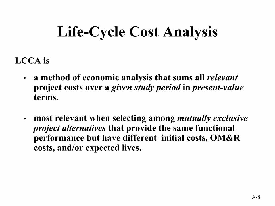
Life-Cycle Cost Analysis

• a method of economic analysis that sums all relevantproject costs over a given study period in present-valueterms.

• most relevant when selecting among mutually exclusive project alternatives that provide the same functional performance but have different initial costs, OM&R costs, and/or expected lives.

LCCA is

A-9

Typical Project Costs

Generally, only amounts that are different need to be considered when comparing mutually exclusive alternatives.

• Investment-related:– Acquisition costs– Replacement costs– Residual value (resale or disposal cost)

• Operating-related:– Operation, maintenance, and repair costs– Energy and water costs– Contract-related costs (for financed projects)

A-10

The Study PeriodThe study period• is the length of time over which an investment is

analyzed based on – the expected life of the project and/or– the investor’s time horizon.

• Base Date: analysis date to which all cash flows are discounted.

• Service Date: date when building or system is occupied or becomes operational.

• Study period must be the same for all alternatives.

A-11

Study Period

Service Period

Study Period

Base Date

Service Date

Year 1 2 3 4 n

Service Period

Study Period

Base Date

Service Date

Year 1 2 3 4 5 6 7 n

Coinciding Study Period and Service Period

Phased-in Planning/Construction/Implementation Period

A-12

Adjusting for Different System Lives

SYSTEM II: 20 YRS

SYSTEM I: 15 YRS

1 2015

Residual

1 2015 30

Replacement Residual

Length of study period

A-13

Present Value and Discounting

• is the equivalent value to an investor, as of the base date, of a cash amount paid or received at a future date.

• is found by discounting; discounting adjusts for the investor’s time-value of money.

A present value amount

The present value of a future amount

• is the interest rate that makes an investor indifferentbetween cash amounts received or paid at different points in time.

The discount rate

A-14

Life-Cycle Cost

Study Period

ReplacementCost

ReplacementCost

ResidualValue

Ope

ratin

gC

osts

Inve

stm

ent

Cos

ts

First Cost

OM&R Costs - Contract Costs

A-15

Converting future amounts to present value:

PV = Ct × 1

LCC = Σn

t=0

Ct

(1+d)t

where n = length of study period.

(1+d)t

A-16

Useful Discount Factors(1) Single present value (SPV) factor for one-time amounts

or non-annually recurring amounts:

(2) Uniform present value (UPV) factor for uniform annual amounts:

where A0 = annual amount at base-date prices

PV = Ft x SPV(t,d)

PV = A0 x UPV(n,d)

A-17

Useful Discount Factors (cont.)

(3) Modified uniform present value (UPV*) factor for changing annual amounts

PV = A0 x UPV*(n,d,e)

A-18

DOE Energy Price Projections

• DOE energy price escalation rates vary– by region (census region)– by fuel type (elec., oil, gas, LPG, coal)– by rate (residential, commercial, industrial)– by year

A-19

Summary of Present Value Factors

PV

PV

PV

Ft

Ao Ao Ao

A1 A2A3

SPV

UPV

UPV*

Single future amount (year t) PV = Ft x SPV (t,d)

Recurring annual amount (over n years) PV = Ao x UPV(n,d)

Changing annual amount (over n years) PV = Ao x UPV*(n,d,e)

A-20

Single Present Value Factor

Example: Find the present value of $1,000 received at the end ofyear 10 when the discount rate is 3.3% (table A-1, Annual Supplement to HB135).

PV = Ft x SPV

PV = $1,000 x SPV (d=3.3%, t=10)

= $1,000 x 0.723 = $723

A-21

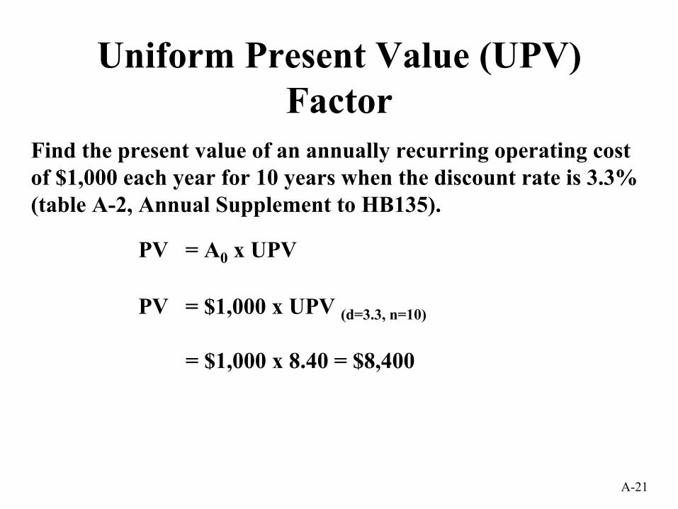
Uniform Present Value (UPV) Factor

Find the present value of an annually recurring operating cost of $1,000 each year for 10 years when the discount rate is 3.3% (table A-2, Annual Supplement to HB135).

PV = A0 x UPV

PV = $1,000 x UPV (d=3.3, n=10)

= $1,000 x 8.40 = $8,400

A-22

Modified Uniform Present Value (UPV*) Factor

Find the present value of an annually recurring operating cost of $1,000 over 10 years, when this cost is expected to escalate at 2%/yr and the discount rate is 3.3% (table A-3a, Annual Supplement to HB135).

PV = A0 x UPV*

PV = $1,000 (annual) x UPV*(d=3.3, n=10, e=2%)

= $1,000 x 9.33 = $9,330

A-23

FEMP UPV* Factor for Energy Costs

Find the present value of an annually recurring electricity costof $1,000 over 10 years, given current DOE energy price escalation rates (Region 4, industrial rates) and the current DOE discount rate of 3.3% (table Ba-4, Annual Supplement to HB135).

PV = A0 x UPV*

PV = $1,000 x UPV*(d=3.3, n=10, electr., industrial, region 4)

= $1,000 x 6.96 = $6,960

A-24

Sources of Discount Factors• Discount factors can be hand-calculated, computer-

calculated, or looked up.• Sources:

– Annual Supplement to Handbook 135 (for federal projects)

– NIST DISCOUNT computer program, NISTIR 85-3273-xx– Generic discount factor tables, NISTIR 89-4203

• Available from:– DOE HELP Desk at 1-800-DOE-EREC (363-3732) or– www.eren.doe.gov - Technical Assistance - Analytical

Software Tools

A-25

Inflation Adjustment in LCCADefinitions

• Inflation: rate of increase of the general level of prices.

• Escalation: rate of increase in the price of a particular commodity.

• Differential escalation: rate of increase in the price of a particular commodity relative to the rate of increase in the general level of prices.

A-26

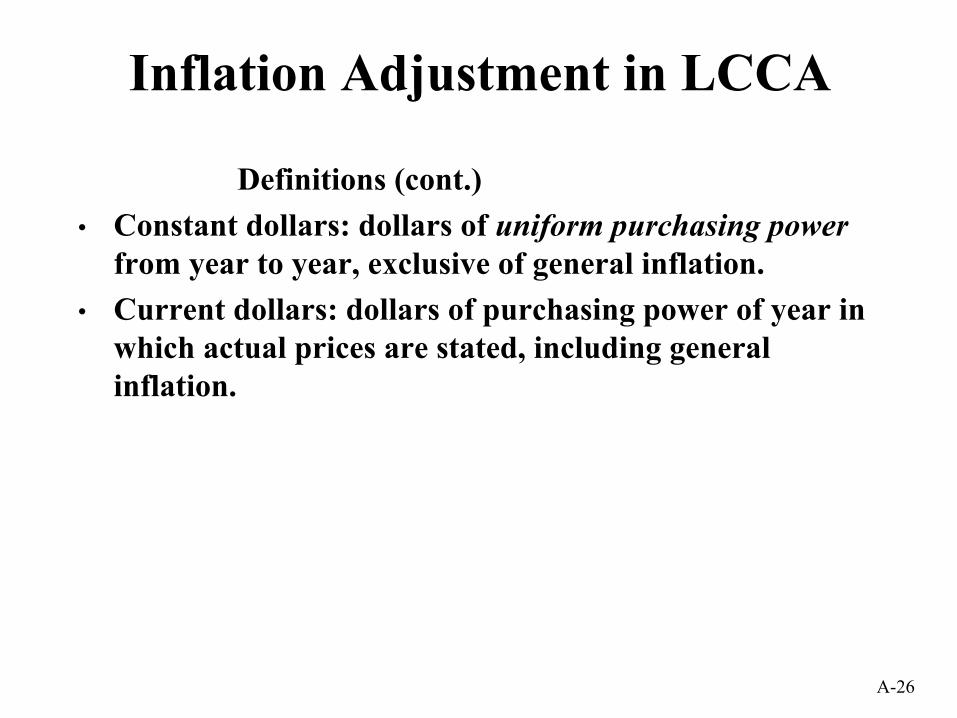
Inflation Adjustment in LCCA

Definitions (cont.)• Constant dollars: dollars of uniform purchasing power

from year to year, exclusive of general inflation.• Current dollars: dollars of purchasing power of year in

which actual prices are stated, including general inflation.

A-27

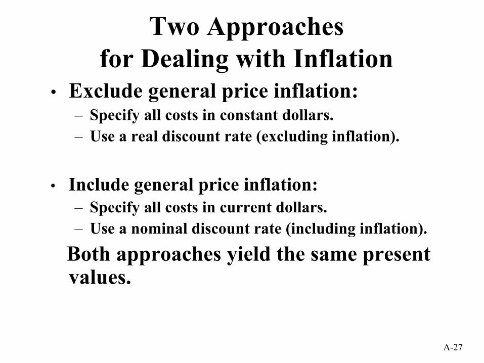
Two Approaches for Dealing with Inflation

• Exclude general price inflation:– Specify all costs in constant dollars.– Use a real discount rate (excluding inflation).

• Include general price inflation:– Specify all costs in current dollars.– Use a nominal discount rate (including inflation).

Both approaches yield the same present values.

A-28

Comparing LCCs of Alternative Systems Requires a Common

Analytical Perspective• Base date• Service date• Study period• Discount rate• Inflation assumption (or constant dollar

analysis)• Cost estimating method(s)• Operational schedule• Energy analysis method

A-29

Federal Criteria for LCC Analysis• Energy and Water Conservation Projects—10 CFR 436A/HB135

– DOE discount rate (updated annually), published in Annual Supplement to Handbook 135

– Maximum 25-year service period– Local energy prices, metered energy quantities– DOE energy price escalation rates– Analysis usually in constant base-year dollars (i.e., excluding inflation),

except for financed projects• Other federal projects—OMB Circular A-94

– OMB discount rates, varying with length of study period and type of project

– No limit on study period

A-30

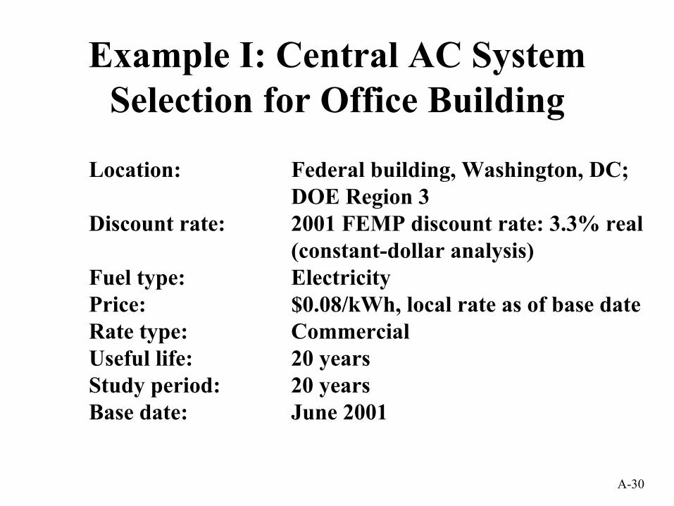
Example I: Central AC SystemSelection for Office Building

Location: Federal building, Washington, DC;DOE Region 3

Discount rate: 2001 FEMP discount rate: 3.3% real(constant-dollar analysis)

Fuel type: ElectricityPrice: $0.08/kWh, local rate as of base dateRate type: Commercial

Useful life: 20 yearsStudy period: 20 yearsBase date: June 2001

A-31

Base Case:Conventional System w/o Computer

Controls and Economizer• $103,000 Initial investment costs

• $ 12,000 Replacement cost for fan at the end of year 12

• $ 3,500 Residual value at the end of the 20-yearstudy period

• $ 20,000 Annual electricity costs (250,000 kWh at $0.08/kWh)

• $ 7,000 Annual OM&R costs

A-32

Cash-Flow Diagram for Base Case

$20,000 annually Electricity

$103,000 Initial

investment cost

$7,000 annually OM&R

Base Date

$12,000 Fan replacement

$3,500 Residual

value

20Year 01 02 03 04 05 06 07 08 09 10 11 12

A-33

LCC for Base Case(Conventional System)

Cost Items

(1)

Base DateCost(2)

Year ofOccurrence

(3)

DiscountFactor

(4)Initial investment $103,000 Base date already in

present valueCapital replacement(fan)

$12,000 12 SPV12 0.677

Residual value ($3,500)) 20 SPV20 0.522

Electricity:250,000 kWh at$0.08/kWh

$20,000 annual UPV*20

12.99OM&R $7,000 annual UPV20

14.47Total LCC

PresentValue

(5)=(2)x(4)$103,000

$8,124

($1,827)

$259,800

$101,290$470,387

A-34

Alternative Case:Energy-Saving System with Computer

Controls and Economizer• $110,000 Initial investment costs

• $ 12,500 Replacement cost for fan at the end of year 12

• $ 3,700 Residual value at the end of the 20-year study period

• $ 13,000 Annual electricity costs (162,500 kWh at $0.08/kWh)

• $ 8,000 Annual OM&R costs

A-35

LCC for Alternative (Energy-saving system)

Cost Items

(1)

Base DateCost(2)

Year ofOccurrence

(3)

DiscountFactor

(4)Initial investment cost $110,000 Base date already in

present valueCapital replacement(fan)

$12,500 12 SPV12 0.677

Residual value ($3,700) 20 SPV20 0.522

Electricity:162,000 kWh at$0.08/kWh

$13,000 annual UPV20* 12.99

OM&R $8,000 annual UPV20 14.47

Total LCC

PresentValue

(5)=(2)x(4)$110,000

$8,462

($1,931)

$168,870

$115,760

$401,161

A-36

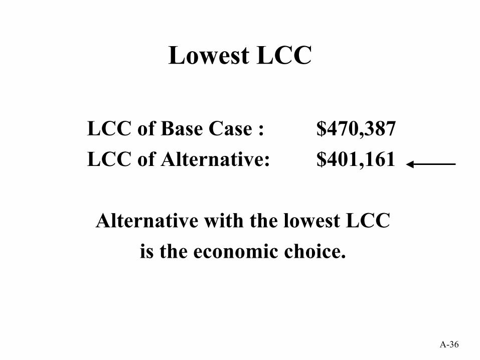
Lowest LCC

LCC of Base Case : $470,387LCC of Alternative: $401,161

Alternative with the lowest LCCis the economic choice.

A-37

Uses of Life-Cycle Cost

Types of Decisions LCC CriterionAccept /Reject yes lowest LCCOptimal Performance yes lowest LCCOptimal System/Design yes lowest LCCProject Priority no ---

A-38

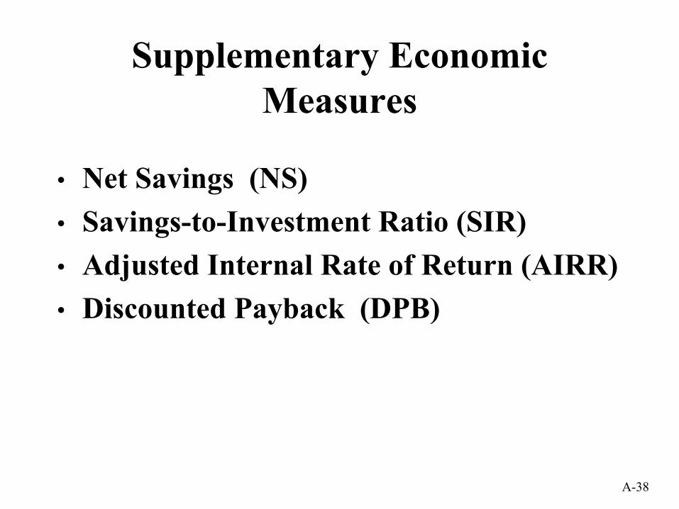
Supplementary Economic Measures

• Net Savings (NS)• Savings-to-Investment Ratio (SIR)• Adjusted Internal Rate of Return (AIRR)• Discounted Payback (DPB)

A-39

Net Savings (NS)

NS = PV of operational savings minus PV of additional investment

NSAlt = LCCBC - LCCALTNSALT = $470,387 - $401,161NSALT = $ 69,226

Alternative with the highest NSis the economic choice.

A-40

Uses of Net Savings

Types of Decisions LCC CriterionAccept /Reject yes > 0 / < 0Optimal Performance yes maximizeOptimal System/Design yes maximize Project Priority no ---

A-41

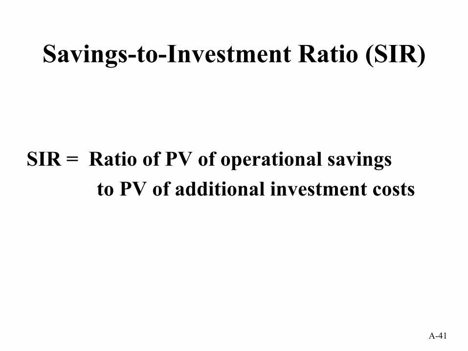
Savings-to-Investment Ratio (SIR)

SIR = Ratio of PV of operational savings to PV of additional investment costs

A-42

Savings-to-Investment Ratio

SIR =PV operational savings

PV Operational savings = PV O&M costsBC - PV O&M costsALTPV∆ Investment costs = PV investmentALT - PV investmentBC

(110,000 + 8,462 - 1,931) - (103,000 + 8,124 - 1,827)SIR =(259,800 + 101,290) - (168,870 + 115,760)

7,234

SIR = 76,460 = 10.6

PV of additional investment costs

A-43

Uses of Savings-to-Investment Ratio

Types of Decisions LCC CriterionAccept /Reject yes > 1 / < 1Optimal Performance no ---Optimal System/Design no ---Project Priority yes descending

orderMeaningful SIR cannot be computed for financed

projects.

A-44

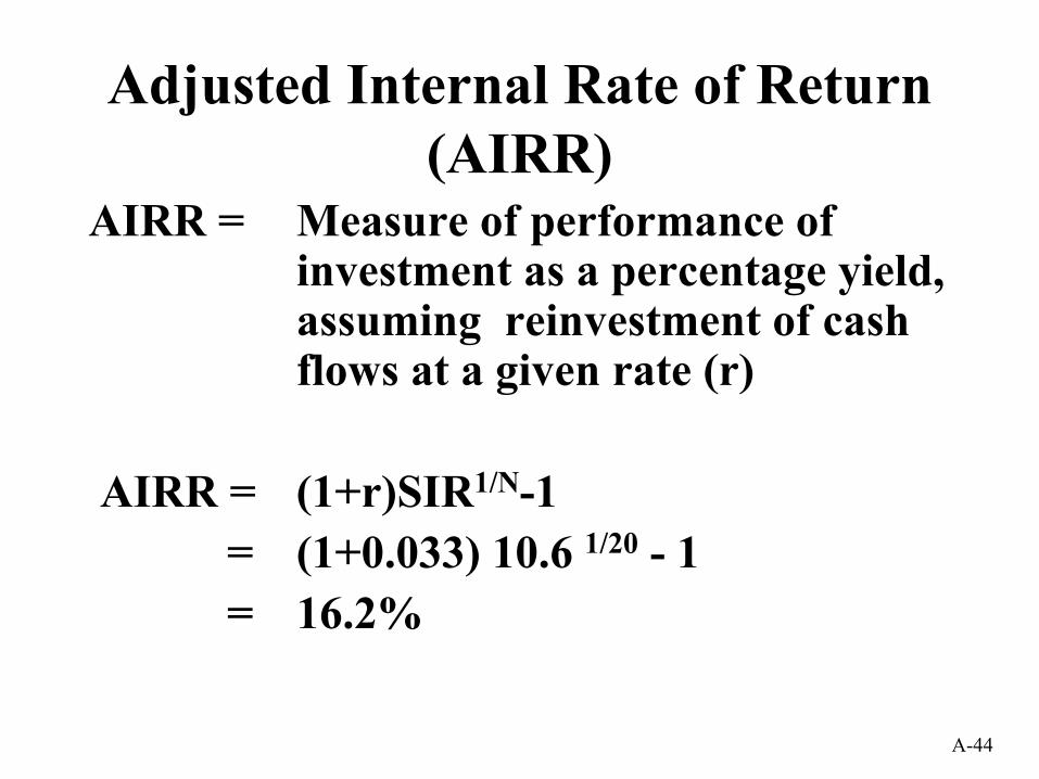
Adjusted Internal Rate of Return (AIRR)

AIRR = Measure of performance of investment as a percentage yield, assuming reinvestment of cash flows at a given rate (r)

AIRR = (1+r)SIR1/N-1= (1+0.033) 10.6 1/20 - 1= 16.2%

A-45

Uses of Adjusted Internal Rate of Return

Types of Decisions LCC CriterionAccept /Reject yes > d / < dOptimal Performance no ---Optimal System/Design no ---Project Priority yes descending

orderMeaningful AIRR cannot be computed for

financed projects.

A-46

Discounted Payback (DPB)

DPB = Minimum value of n, years, for which discounted savings in year t are at least equal to additional initial investment costs

( )( )S I

dIt t

tt

n −

+≥

=∑ ∆∆

110

A-47

Discounted Payback for Alternative

Base-year electricity savings: $7,000Base-year OM&R savings: - $1000Additional Initial Investment: $7,000

Cumulative ∆Initial CumulativeYear PV Savings Cost PV Net Savings1 $ 5,610 $7,000 -$1,3902 10,970 7,000 3,970

Discounted Payback occurs in year 2.

A-48

Uses of Discounted Payback

Types of Decisions LCC CriterionAccept /Reject yes ≤ / ≥ proj.life Optimal Performance no ---Optimal System/Design no ---Project Priority no ---

Meaningful DPB cannot be computed for financed projects.

A-49

• 2-year planning/construction period

• First half of investment cost incurred at end of year 1, second half at service date

Example II: CAC System Selection for Office Building with

Planning/Construction Period

A-50

Cash Flow Diagram for Base Case with P/C Period

Electricity

$51,500

$51,500

$7,000 OM&R

Base Date

Service Date

$12,000 Cap. repl.

(fan)

$3,500 Residual

value

Year 01 0302 12 18 22

Initial investment costs

$20,000

07

A-51

LCC Calculation for Base Case with P/C Period

Cost Items

(1)

Base DateCost(2)

Year ofOccurrence

(3)

DiscountFactor

(4)Initial investment cost:

$51,500 1

Capital replacement (fan) $12,000 14 SPV14 0.635Residual value ($3,500) 22 SPV22 0.490Electricity:250,000 kWh at$0.08/kWh

$20,000 annualUPV*

22-2

OM&R $7,000 annual UPV22-2

Total LCC

PresentValue

(5)=(2)x(4)

$49,852

$7,620($1,715)

$240,800

$94,920$439,733

1st Installment atmidpoint of construction

SPV1 0.968

$51,500 2 $48,2562nd Installment atbeginning of serviceperiod

SPV2 0.937

13.88-1.84 = 12.04

15.47-1.91 = 13.56

A-52

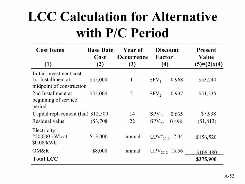
LCC Calculation for Alternative with P/C Period

Cost Items

(1)

Base DateCost(2)

Year ofOccurrence

(3)

DiscountFactor

(4)Initial investment cost:

$55,000 1

Capital replacement (fan) $12,500 14 SPV14 0.635Residual value ($3,700) 22 SPV22 0.490Electricity:250,000 kWh at$0.08/kWh

$13,000 annual UPV*22-2 12.04

OM&R $8,000 annual UPV22-2

Total LCC

PresentValue

(5)=(2)x(4)

$53,240

$7,938($1,813)

$156,520

$108,480$375,900

1st Installment atmidpoint of construction

SPV1 0.968

$55,000 2 $51,5352nd Installment atbeginning of serviceperiod

SPV2 0.937

13.56

A-53

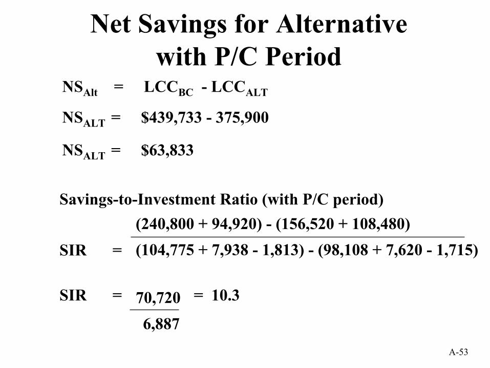
Net Savings for Alternative with P/C Period

NSAlt = LCCBC - LCCALT

NSALT = $439,733 - 375,900

NSALT = $63,833

Savings-to-Investment Ratio (with P/C period)

(104,775 + 7,938 - 1,813) - (98,108 + 7,620 - 1,715)SIR =(240,800 + 94,920) - (156,520 + 108,480)

6,887

SIR = 70,720 = 10.3

A-54

Class Exercise A1Attic Insulation

Materials required: Annual Supplement to Handbook 135Four-function calculator

Note: These problems are intended for manual solution.

Use the worksheet on the next page to determine the level of insulation with the lowest life-cycle cost, which is to be installed in the attic of a house located in Northern California. The existing insulation level is R-11.Location: West (Region 4)Base date: June 2001Service date: June 2001Discount rate: 3.3%Expected life: 25 yearsReplacements: noneResidual value: noneElectricity price: 0.08/kWhRate type: Residential

Insulation Annual energy consumption InstalledCost ($)Level

R-11R-19R-30R-38

kWh9602705568046703

0450650800

A-55

Worksheet for Class Exercise A1

(1) (2) (3) (4)= (5) (6)= (7)= (8)=(3)X$.08/kWh (4)x(5) (2)+(6) LCCR-0 – LCCR-N

Energy CostR-

value

InitialCost($)

AnnualkWh

Annual($) UPV*

Life($)

TotalLCC($)

NetSavings

($)

R-11

R-19

R-30

R-38

0

450

650

800

9602

7055

6804

6703

A-56

Class Exercise A2Selection of Heating System

Select the residential heating system with the lower life-cycle cost and calculate its Net Savings and Savings-to-Investment Ratio. Use the worksheet on the next page.

Annual space heating load: 50 MBtuFuel oil price: $1.12/gallon ($8.00/MBtu)Natural gas price: $0.80/therm ($8.00/MBtu)Rate type: ResidentialLocation: Midwest (Region 2)Discount rate: 3.3%Base date/service date: June 2001Study Period: 15 years

Oil Furnace Gas FurnaceInitial cost: $4,500 $5,000Annual maintenance cost $100 $75Annual efficiency (average) 82% 83%Expected life (years) 15 15Residual value $500 $1,000

A-57

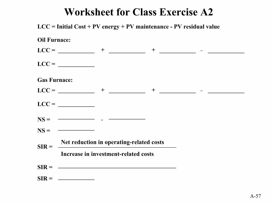
Worksheet for Class Exercise A2LCC = Initial Cost + PV energy + PV maintenance - PV residual value

Oil Furnace:

LCC = + + –

LCC =

Gas Furnace:

LCC = + + –

LCC =

SIR =Net reduction in operating-related costs

Increase in investment-related costs

SIR =

SIR =

NS = -

NS =

A-58

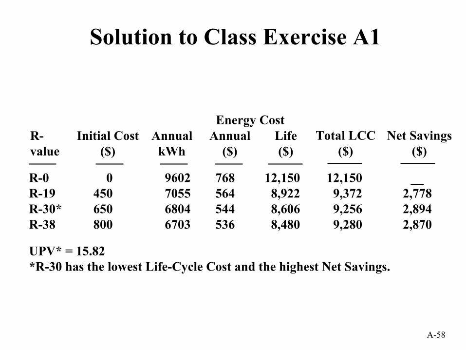
Solution to Class Exercise A1

UPV* = 15.82*R-30 has the lowest Life-Cycle Cost and the highest Net Savings.

Annual($)

Life($)

Initial Cost($)

AnnualkWh

R-value

Energy Cost

12,1508,9228,6068,480

0450650800

9602705568046703

Total LCC($)

Net Savings($)

__2,7782,8942,870

12,1509,3729,2569,280

768564544536

R-0R-19R-30*R-38

A-59

Solution to Class Exercise A2Lowest Life-Cycle Cost:

LCC = Initial Cost + PV energy + PV maintenance - PV residual value

Oil Furnace:LCC = $4,500 + (50/0.82 x $8.00 x 10.66) + ($100 x 11.68) - ($500 x 0.614)LCC = $4,500 + $5,200 + $1,168 - $307LCC = $10,561

Gas Furnace:LCC = $5,000 + (50/0.83 x $8.00 x 10.16) + ($75 x 11.68) - ($1,000 x 0.614)LCC = $5,000 + $4,896 + $876 - $614LCC = $10,158

Net Savings for Gas Furnace:NS = $10,561 - $10,158NS = $ 403SIR for Gas Furnace:SIR = ($5,200 + $1,168) - ($4,896 + $876)

($5,000 - $614) - ($4,500 -$307)

SIR = $ 596 $ 193

SIR = 3.09

A-60

Summary of the Life-Cycle Costing Method

Savings and investment costsThe basic criterion for determining whether a design alternative that increases capital investment andlowers future operating costs is cost-effective is that the savings generated by the investment mustbe greater than the additional investment cost. The number of years over which the savings areaccumulated and the weighting of future costs (or cost savings) relative to present costs are majorconsiderations in life-cycle cost (LCC) analysis.

Life-cycle costThe LCC concept requires that all costs and savings related to a design decision be evaluatedover a common study period and be adjusted for the time value of money before they can bemeaningfully compared. Choosing building systems on the basis of first cost alone can increase thelong-run owning and operating costs of a building. For example, the purchase of a low-efficiencyheating system, while initially less expensive than a more efficient system, will incur higher energycosts when in use. The difference may be significant since for many building systems only a smallpart of the life-cycle cost is attributable to the initial purchase price. The greater part is usuallyattributable to ongoing operating, maintenance, repair, and energy costs.

The principles of present-value analysis, which are the basis for the life-cycle cost method, apply toinvestments in federal, state, and local governments whether they are funded by the governmentagency from tax appropriations or financed through private-sector energy or utility servicescompanies.

To supplement LCC analysis, there are additional measures of economic effectiveness, such asNet Savings (NS), Savings-to-Investment Ratio (SIR), Adjusted Internal Rate of Return (AIRR)and Discounted Payback Period (DPB) period. If computed correctly, all of these measures areconsistent with the LCC method.

Particular care must be given to the use of the DPB as a criterion for accepting or rejectingprojects. The DPB is consistent with the LCC method only when nothing more is required than thatpayback occur before the end of the study period and if cumulative net savings after payback isachieved are positive. DPB is not consistent with the LCC method when an arbitrary payback periodis specified as a cut-off point for project acceptance.

Comparing alternativesFrom a decision standpoint, the LCC of a design alternative only has meaning when it iscompared against the LCC of a base case. For example, Alternative B has a higher investment costbut lower operating-related costs than Base Case A, although both are expected to perform equallywell with regard to their basic purpose. Since the sum of investment cost plus operating cost(including energy costs) for alternative B is less than that for A, alternative B is the more cost-effective choice. Note that in an existing building, the base case alternative (i.e., the existing design)may not require any investment; it may be the "do nothing" alternative. In that case, the life-cyclecost of the base case is made up entirely of operating-related costs, which must be compared againstthe combined investment and operating costs of the alternatives considered. In other cases (e.g., a

A-61

new building design) the base case may be the design with the lowest first cost or the minimum levelof performance that satisfies building code requirements.

Minimizing total owning and operating costsThe graph in slide A-5 is typical of energy conservation investments. It compares the owningand operating costs associated with a wide range of energy efficiency levels for a buildingsystem (e.g., exterior wall insulation or air conditioner efficiency). Generally, as the level ofenergy efficiency increases, the initial cost increases at an increasing rate. Lower levels ofefficiency can generally be achieved at low cost, but as the efficiency level is increased,structural, mechanical, or design modifications must be made to accommodate the addedcomponents. This quickly adds to the initial cost. For example, to increase the effective thermalresistance value of a wall, the wall thickness must be increased or a more costly type ofinsulation must be used; or, in the case of air conditioners, significantly larger heat exchangers ormore costly compressors are necessary to increase energy efficiency. For some systems, such asfossil-fired furnaces, there are practical limits to the extent to which efficiency can be increased,causing the investment cost curve to bend sharply upwards.

The operating cost curve in the graph shows that as the energy efficiency of the system is increased,energy consumption is decreased, but at a decreasing rate. In fact, energy consumption is generallyinversely proportional to energy efficiency so that additional units of improvement generate lesssavings than the ones before. For example, increasing the thermal resistance value of attic insulationfrom R-30 to R-40 only saves about 18 % as much energy as increasing the level from R-10 to R-20.

The total cost curve is the vertical summation of the investment cost and operating cost associatedwith any level of energy efficiency. The lowest point on the total cost curve, Q*, determines thelevel of energy efficiency that minimizes life-cycle costs. It is important to recognize that there area number of factors that contribute to this result. For example, longer study periods, more severeclimates, lower conservation costs (say through technology improvements), and higher energy pricesall tend to result in a higher level of energy efficiency becoming cost-effective.

Maximizing net savingsThe graph in slide A-6 shows that the most cost-effective level of energy conservation can also bedetermined by finding the level that maximizes net savings, the difference between total costs andtotal savings. The slide shows two curves, the investment cost curve, which is identical to that shownin the previous slide, and a savings curve. The savings curve is determined by taking the differencebetween the operating cost at the zero level of investment and the operating cost at any other level ofinvestment on the graph.

Note that total savings are greater than total costs anywhere between the origin and the point wherethe two curves cross. Thus we might conclude that any level of investment between these two pointsis justified. But in fact the economically optimal level of energy efficiency is that level for whichnet savings is greatest, again Q*. This is the same point that was determined by finding the levelwith the lowest LCC. This is not surprising if you recognize that net savings at any point along thehorizontal axis of the graph in slide A-5 is the difference between the LCC of the base case(measured at the zero investment level) and the LCC of the alternative at that point. Thus the energyefficiency level with the lowest LCC must have the highest net savings. By contrast, at the point

A-62

where investment cost just equals savings (slide A-6), you are no better off than you were at theorigin, since in both cases net savings is zero.

Incremental savings versus incremental costsGraph A-7 provides an additional look at the relationship between the investment cost curve and theoperating cost curve. Here incremental costs and incremental savings are plotted. Each additionalunit of energy efficiency results in smaller and smaller increments in savings and greater and greateradditions to cost. The shape of these curves is quite typical: conservation investment costs areincreasing at an increasing rate and energy savings are decreasing at a decreasing rate. The pointwhere these two curves cross determines the economically optimal level of energy efficiency,again Q*, the point at which the last increment in cost increases savings by the same amount.This is the same point, Q*, found by minimizing LCC or maximizing net savings. At any point to theleft of Q*, incremental savings are higher than incremental costs, so that increasing the energyefficiency level will reduce life-cycle costs and increase net savings. At any point to the right of Q*,the intersection, incremental savings are less than incremental costs, so that reducing the energyefficiency level will reduce life-cycle costs and increase net savings.

Economic efficiencyIt is essential to recognize that all three of these methods arrive at the same optimal level of energyefficiency. In general, if the LCC methodology is applied correctly, all three of these methodsarrive at the same optimal level of energy efficiency. Economists refer to the level of investmentwhere life-cycle cost is minimized, net savings is maximized, and incremental investment is equal toincremental savings as the "economically efficient" level of investment for a given project.

The above treatment of costs and savings assumes that the energy efficiency of building systems canbe improved in a continuous fashion. In fact, commercially available systems are rarely available in acontinuous range of efficiency ratings. However, the underlying concepts shown here are valid evenwhen efficiency improvements come in "step" form. That is, the alternative with the lowest LCCwill be the most cost-effective choice, given that it satisfies the other performance objectives of thesystem. In every case, finding the alternative with the lowest LCC will provide sufficientinformation to choose the economically efficient level of investment.

Types of decisionsThere are five types of investment decisions related to energy conservation to which economicanalysis can be usefully applied:

(1) An accept/reject project is a project that is optional from a building design standpoint and canbe either implemented or not, depending on whether or not it is a good investment. A goodexample is the installation of standard storm windows over existing single-pane windows in ahouse. The comfort level of a house can be maintained at an acceptable level with or withoutstorm windows, but with storm windows installed much less energy will be used. (If severaloptions are available with different levels of energy performance, then this becomes a decisionabout the optimal efficiency level.) Optimal efficiency level refers to the problem of selectingthe most cost-effective level of energy performance for a building system. For example, atticinsulation can be installed over a wide range of thermal resistance levels, an air conditioner canhave a wide range of seasonal efficiency ratings, and a solar heating system can have a widerange of collector areas.

A-63

(2) Optimal system selection refers to the problem of selecting the most cost-effective system type

for a particular application. System selection can directly impact the energy performance of abuilding. Examples include the choice of the heating and cooling system types for a building(e.g., electric heat pump or gas furnace with electric air conditioning), wall design (e.g., masonryor wood frame), or even insulation type (e.g., rigid foam or mineral wool).

(3) Optimal combination of interdependent projects refers to the problem of selecting two or

more building systems at the same time, recognizing that the implementation of one system willhave significant effects on the energy savings potential of the other, and vice-versa. Forexample, installing a high-efficiency furnace will reduce the energy savings potential of stormwindows, while installing storm windows will reduce the energy savings potential of installing ahigh-efficiency furnace.

(4) Prioritization of independent projects is required when a number of cost-effective energy

conservation investments have been identified but not enough funding is available to implementall of these projects. Economic analysis allows the ranking of these projects in decreasing orderof cost-effectiveness as a guideline to allocating available funding.

Basic steps in LCC analysisThe basic steps in an LCC analysis are to- identify the alternatives under consideration,- specify the data requirements and establish assumptions,- estimate the costs in dollars,- adjust costs for time value of money,- compute total LCC for each alternative, and- choose the alternative with the lowest total life-cycle cost.

Depending on the circumstances, you may also want to calculate supplementary measures ofeconomic performance, perform an uncertainty assessment, and add a narrative describing non-economic issues. All of these steps will be covered during the workshop.

Typical project costsRelevant effectsTo make a decision about economic efficiency, it is important to measure the economicconsequences of alternatives. Data requirements for making an economic decision are not the sameas those for keeping an accounting system. For an LCC analysis, you need, in general, evaluate onlycosts that change from one alternative to another. Costs that remain the same do not decrease orincrease the life-cycle costs of an alternative relative to the base case and thus need not be included.

Because collecting cost data can be expensive, you want to focus on collecting those data which arelikely to have a significant effect on the life-cycle costs of an alternative. You do not want to spendyour limited resources on collecting data that have little impact.

A-64

Do not include "sunk" costs in your analysis. Sunk costs are those costs that have already beenincurred and cannot be avoided by future decisions. Only amounts that can be changed by thedecision need to be included in the analysis.

Non-tangible costs are costs or benefits that cannot easily be expressed in dollar amounts. Eventhough they cannot be explicitly included in an LCC analysis, their effects should be described in anarrative so that they will not be overlooked when making a decision.

Types of costsLife-cycle costs typically include investment-related costs and operational costs. Acquisitioncosts, including costs for planning, design, and construction, are investment-related, as are residualvalues such as resale value, salvage value, or disposal costs. Under the FEMP rule, capitalreplacement costs are also defined as investment-related. Energy costs, maintenance costs, andrepair costs are considered operational costs, that is, non-investment-related costs. This definition isuseful when computing economic measures that evaluate long-run savings in operational costs inrelation to total capital investment costs.

Some of the costs included in an LCC analysis are annually recurring, such as energy, and routinemaintenance and repair costs. Non-annually recurring costs are those that may occur only one timeduring the life-cycle, such as acquisition costs and residual values, or several times, such asreplacement costs. This definition is needed for choosing the appropriate discount factors used toconvert future costs to present values.

In a third classification, acquisition costs are designated as initial costs and all other costs as futurecosts, a useful classification both for selecting discount factors and for relating initial investmentcosts to the operating costs of a project.

All costs included in the analysis are expressed in base-year dollars. These base-year amounts willbe multiplied by discount factors that incorporate the discount rate and any applicable escalationrate.

Energy and water costsSpecial criteria apply to energy costs in analyses of conservation measures considered for federalbuildings:

Current prices: It is essential to get current energy prices from local suppliers. It is better not to useregional or national average energy or water cost data, since they do not reflect local supply anddemand conditions. Prices should take into account, where applicable, rate type, rate structure,summer and winter differentials, block rates, and demand charges to reflect an estimate as close aspossible to today's actual price.

Energy price projections: Energy prices are assumed to increase or decrease at a rate different fromgeneral price inflation. To avoid inconsistencies in LCC analyses throughout the government, it isrequired under the FEMP rule (10 CFR 436A) to adjust today's energy price estimates by the energyprice projections published annually by DOE. These energy price projections are embedded in thediscount factors updated annually and published on April 1 of each year in Energy Prices andDiscount Factors for Life-Cycle Cost Analysis 20xx, Annual Supplement to NBS Handbook 135 and

A-65

NBS Special Publication 709. These projections are also included in the NIST BLCC computerprograms.

Water costs: In 1995 water conservation was added to energy conservation as a designated goal forthe Federal Energy Management Program. No special water usage/disposal escalation rates areprojected by DOE.

Setting the study periodThe study period is the time over which the effects of a decision are of interest to the decision-maker.There is no one correct study period, but it must be sufficiently long to enable a correct assessment oflong-run economic performance. Often the life of the system under analysis is used as the studyperiod. However, the Federal Government limits the study period for energy and water conservationprojects to a maximum of 25 years from the service date. Apart from the 25-year maximum limit,there are other factors that determine the length of the study period:

(1) Compare all alternatives over the same study period. Present-value cash flows calculatedfor one time period would not be comparable with those calculated for a longer or shorterperiod.

(2) Calculate all measures of economic evaluation (LCC, NS, SIR, AIRR) using the samestudy period, otherwise they would not be consistent with each other.

(3) Consider the time horizon of the investor. The study period may be shorter or longerdepending on whether the investor is, for example, the builder or the occupant of a building.

(4) Adjust for different expected lives of buildings or systems. In order to fit differentexpected lives into the same study period, equalize the differing time periods by usingreplacement values and residual values, such as a resale value, salvage value, or disposalcosts.

Discounting future costs to present valueBefore we can compare or sum costs occurring at different points over the study period, they must beconverted to a common point in time to reflect the time value of money. This means that future costs(or savings) have to be discounted to present value so that they can be directly compared withinitial investment costs.

Cash-flow conventionsThere are several cash-flow conventions that may be used when discounting costs occurring over thestudy period to present value. One-time costs are usually discounted from the actual time ofoccurrence. Annually recurring costs are discounted from the end of the year (FEMP) or the middleof the year (DoD). Costs occurring at the beginning of the study period do not need to be discountedsince they are already in present value.

Discount rateThe discount rate used to adjust future costs to present value is the rate of interest that makes theinvestor indifferent between cash amounts received at different points in time. The discount rateadjusts for inflation and the real earning power of money. This rate is often referred to as the

A-66

minimum acceptable rate of return (MARR). It is important to recognize that every investor hashis or her own time preference for money, and thus his or her own discount rate.

Discount factorsPre-calculated discount factors can be used to calculate present values by multiplying the base-yeardollar amounts by the appropriate discount factor. NIST publication Discount Factor Tables for Life-Cycle Cost Analyses (NISTIR 89-4203) contains pre-calculated discount factors that incorporateFEMP and OMB discount rates and DOE energy price escalation rates. These discount factors arealso embedded in the NIST BLCC programs.

Common discount factor applicationsWhen performing an LCC analysis, three types of future cash flows are most commonly encountered,each requiring a different type of present-value factor:

(1) The one-time cash flow is multiplied by the Single Present Value (SPV) factor to find itspresent value. An example of a one-time cash flow is a replacement cost or a residual value atthe end of the study period.

(2) The uniform annual amount is multiplied by the Uniform Present Value (UPV) factor to find

the present value. An example of a uniform annual amount is an annual operating andmaintenance cost that remains the same from year to year.

(3) The changing annual amount varies from year to year at some known rate, which can be either

constant or variable from year to year. The base-year amount (A0) is multiplied by the ModifiedUniform Present Value (UPV*) factor to find the present value. An example of an amount thatchanges at a variable rate each year is the annual energy cost of a building when the physicalamount of energy consumed is expected to be reasonably constant but energy prices are expectedto change from year to year. An amount changing at a constant rate may be an operating cost thatincreases annually due to expected higher maintenance costs.

UPV* factors for energy costsFor LCC analyses related to energy conservation in federal facilities, NIST publishes UPV* factorsspecifically for use with future energy costs. The NIST UPV* factors explicitly incorporate theFEMP discount rate and DOE projections of energy price increases over the next 30 years. They arepublished in NISTIR 85-3273, Energy Price Indices and Discount Factors for Life-Cycle CostAnalysis 20xx, tables B-1a through B-5a. Because the FEMP discount rate and the DOE projectionsof energy price escalation rates change from year to year, this publication is updated by NIST eachyear on April 1. The UPV* factors in this publication are differentiated by fuel type, rate type(residential, commercial, industrial), and by region (Northeast, Midwest, South, and West). TheUPV* factor for energy costs is used with the annual energy cost computed in base-year dollars

How to handle inflation in LCC analysisDefinitionsAn economic evaluation of capital investments over time needs to consider both the earningpower of money, as reflected by the discount rate, and the changing purchasing power of the

A-67

dollar. The following five terms will be used in the discussion of how to handle inflation in life-cycle cost analysis:

- Price inflation: A rise in the general price level, tantamount to a decline in the general purchasing power of the dollar.

- Price escalation: Increase in the price of a particular commodity, such as energy.

- Differential price escalation: The difference between the rate of general inflation and

the rate of escalation in the price of a particular commodity. For example, if the price of a particular commodity increases at exactly the same rate as general inflation, the differential price escalation rate is 0 percent. Energy prices are a type of cost that has deviated significantly from general inflation since the early 1970s. For this reason, the FEMP LCC methodology for evaluating energy conservation investments requires that projected increases in energy prices be explicitly included in the economic analysis, while other categories of costs are generally assumed to increase at the rate of general inflation.

- Current dollars and constant dollars: Current dollars include the rate of general

price inflation, constant dollars exclude the rate of general price inflation.

- Nominal discount rates and real discount rates: Nominal discount rates include the rate of general price inflation, real discount rates exclude the rate of general price inflation.

Treatment of inflation There are two basic approaches for dealing with inflation in an economic analysis. (1) Use current dollars and a nominal discount rate and price escalation rates. The rate of

inflation is included in the future dollar amounts, and in the discount and price escalation rates. This is the approach that is generally used when tax considerations are included in the economic analysis, or when current-dollar cash flows need to be compared with current-dollar savings, as is the case for ESPC projects.

(2) Use constant dollars and a real discount rate and price escalation rates. Future dollar

amounts exclude, and the discount and escalation rates exclude inflation. In this case only differential price escalation rates are included in the analysis, exclusive of general inflation. Constant-dollar analyses are generally used in agency-funded government studies.

Both constant- and current-dollar analyses, if conducted properly, will yield exactly the same present-value result, and thus support the same conclusion. However, it is generally easier to conduct an economic analysis in constant dollars because the underlying rate of inflation from year to year over the study period does not need to be estimated. It is important to differentiate between a present-value analysis of a capital investment and a budget analysis, where funds must be appropriated for year-to-year disbursement. The purpose of a present-value analysis is to determine whether the overall savings appear to justify the required investment at the time that the investment decision is being made. A budget analysis must include

A-68

general inflation to assure that sufficient funding will be appropriated in future years to cover actual expenses. Relationship between real and nominal rates:

d = (1 + D)/(1 + I) - 1 D = (1 + d) (1 + I) - 1 e = (1 + E)/(1 + I) - 1 E = (1 + e) (1 + I) - 1

where d = real discount rate, excluding inflation

D = nominal discount rate, including inflation e = real rate of escalation, excluding inflation E = nominal rate of escalation, including inflation I = rate of inflation

Supplementary measures of economic performance Supplementary measures of economic performance can be used to determine the comparative cost-effectiveness of capital investment. Several widely used measures are presented in this workshop. These are Net Savings, Savings-to-Investment Ratio, Adjusted Internal Rate of Return, and Payback Period. Except for the Payback Period, these measures are consistent with and build upon the Life-Cycle Cost methodology. All of these supplementary measures are comparative rather than absolute measures of performance because they are only meaningful in relation to an alternative course of action, i.e., the base case. Net Savings (NS) NS is a measure of long-run profitability of an alternative relative to a base case. The NS can be calculated as an extension of the LCC method to show the difference between the LCC of a base case and the LCC of an alternative. It can also be calculated directly from differences in the individual cash flows between a base case and an alternative. The NS can be used like the LCC measure to determine a project’s cost-effectiveness. For a project alternative to be cost-effective with respect to the base case, it must have an NS of greater than zero. Even with a zero Net Savings, the minimum required rate of return (MARR) has been achieved because the required rate of return is built into the net savings computation through the discount rate. NS is not useful for ranking projects. Savings-to-Investment Ratio (SIR) The SIR is a dimensionless measure of performance that expresses the ratio of savings to costs. The numerator of the ratio contains the operation-related savings; the denominator contains the increase in investment-related costs. An SIR > 1.0 means that an alternative is cost-effective relative to a base case. For selecting the optimal energy efficiency level or the optimal system or design, the SIR method is reliable only if based on incremental SIRs. The SIR is recommended for setting priority among projects when the budget is insufficient to fund all cost-effective projects. The projects are ranked in descending order of their SIRs.

A-69

Adjusted Internal Rate of Return (AIRR) The AIRR is calculated as a percentage yield. The yield rate is compared with the investor’s MARR. The AIRR has to be higher than the MARR for an investment to be considered cost effective. (The AIRR is a modified version of the Internal Rate of Return (IRR); it uses the discount rate rather than the calculated rate of return as the reinvestment rate for saved cash flows.) The AIRR is used in the same way as the SIR. Discounted Payback (DPB) The DPB measures how long it takes to recover initial investment costs. It is calculated as the number of years elapsed between the initial investment and the time at which cumulative savings, net of accrued costs, are just sufficient to offset investment costs. The DPB takes the time value of money into account by using discounted cash flows. If the discount rate is assumed to be zero, the method is called Simple Payback (SPB), a measure of evaluation less accurate than the DPB. Both the DPB and the SPB ignore all costs and savings that occur after payback has been reached. They should be used only as a rough screening measure for accept/reject decisions. Uncertainty assessment in LCC analysis Decisions about energy conservation investments in buildings typically involve a great deal of uncertainty about their costs and potential savings. Performing an LCC analysis greatly increases the likelihood of choosing an alternative that saves money in the long run. Yet, there may still be some uncertainty associated with the LCC results; LCC analyses are usually performed early in the design process when only estimates of costs and savings are available rather than certain dollar amounts. Uncertainty in input values creates risk that a decision will have a less favorable outcome than what is expected. Even though you may be uncertain about some of the input values, especially those occurring in the future, it is still better to include them in an economic evaluation than to base your evaluation on first costs only. Ignoring uncertain long-run costs implies the assumption that they are zero, a poor assumption to make. There are techniques that allow you to estimate the cost of choosing the “wrong” alternative. Sensitivity analysis and breakeven analysis are two approaches that are so simple to perform that they should be part of every LCC analysis. These and a number of other approaches to risk and uncertainty assessment are described in detail in Techniques for Treating Uncertainty and Risk in the Economic Evaluation of Building Investments by Harold E. Marshall, NIST Special Publication 757, September 1988. Sensitivity analysis Sensitivity Analysis measures the impact on the analysis results of changing one or more key input values about which there is uncertainty. Sensitivity analysis can be performed with respect to any measure of worth (LCC, NS, SIR, AIRR, PB). The sensitivity of these measures can be compared among alternatives.

A-70

Identifying critical inputs: It is important to know which of the uncertain input parameters have the greatest effect on LCC results. To identify the critical inputs, simply increase the value of each of them in turn by a certain percentage and, holding all others constant, recalculate the economic measure to be tested. The higher the percentage change in outcome for a given change in input value, the greater the effect. Estimating the range of results: To arrive at an estimate of the upper and lower bounds of an economic measure, it can be recalculated using the lowest and highest likely estimates of its input variables, corresponding to the most optimistic or pessimistic scenarios. “What if” scenarios: Identifying critical input values and determining the range of economic measures answers a number of “what if” questions. Sensitivity analysis is a good technique for taking a closer look at the most plausible “what if” scenarios, in order to be prepared to answer these types of questions when they arise during the decision-making process. Breakeven analysis Decision makers sometimes want to know the maximum cost of an input that will allow the project to still break even, or, conversely, what minimum benefit a project can produce and still cover the cost of the investment. To perform breakeven analysis, benefits and costs are set equal; all variables are specified, except the breakeven variable; and the breakeven variable is solved for algebraically. Advantages and disadvantages of sensitivity and breakeven analyses Results of sensitivity analysis and breakeven analysis can be presented in text, tables, or graphs. They are easy to perform and easy to understand and require no additional methods of computation beyond those needed for LCC analysis. The breakeven value can serve as a benchmark value to be compared against its predicted performance. The disadvantages of sensitivity analysis and breakeven analysis are that they do not give a probabilistic measure of the risk of choosing an uneconomic project and do not include an explicit measure of risk attitude. Summary of FEMP LCC criteria The following criteria, consistent with the FEMP rules outlined in 10 CFR 436A, specifically apply to the economic evaluation of energy and water conservation and renewable energy projects in federal buildings: Constant-dollar analysis In general, use constant dollar analysis and real discount and escalation rates. The DOE/FEMP discount rate and energy price escalation rates are real rates, that is, they exclude the rate of general price inflation. If, as for example, in the case of alternative financing projects, the analysis is performed in current dollars, the inflation rate has to be added to the discount rate and price escalation rates. The DOE discount rate and corresponding discount factors are updated annually on April 1 and published in NISTIR 85-3273, Energy Price Indices and Discount Factors for Life-Cycle Cost Analysis, the Annual Supplement to NIST Handbook 135, and in the NIST LCC computer programs, BLCC4 and BLCC5.

A-71

Discounting convention Cash flows are discounted from the end of the year. (In analyses of military construction projects, cash flows are discounted from the middle of the year.) Present values For reasons of consistency, the FEMP rule prescribes the use of present-value analysis for evaluating energy- and water-related projects. All future dollar amounts should be discounted to the base date of the project. Note that “present-value” amounts are not the same as constant dollar amounts as of the base date, since the latter do not reflect the time value of money. Energy prices The FEMP LCC method uses local energy and water prices at the building site in calculating the annual dollar value of the energy or water consumed by a building or building system. Local energy and water prices should reflect the type of rate charged (residential, commercial, or industrial), differences between summer and winter rates, the impact of block rates on marginal energy and water costs, and demand charges. The analyst should not artificially adjust energy or water prices to reflect environmental externalities. If fuel is purchased for on-site electricity generation, the costs of the fuel at the point of generation, plus the costs incurred in generating and distributing the electricity, should be used in the analysis. Quantity of energy and water usage Since the FEMP LCC method uses local energy and water prices at the building site, energy and water quantities should be stated in units consistent with unit prices at the point of metering. Equivalent quantities of energy or water at some earlier point in the supply chain (e.g., oil or coal prices before conversion to electricity) should not be used. DOE energy price escalation rates Energy prices are assumed to change at rates different from the rate of general price inflation. DOE annually projects real (differential) energy price escalation rates for the next three years, by Census region, rate type, and fuel type. These real energy price escalation rates and the real DOE discount rate are used to calculate the modified present value factors (UPV* factors) for use in FEMP LCC analyses. The UPV* factors are updated and published annually as a set of tables in NISTIR 85-3273, the Annual Supplement to Handbook 135. At present there are no equivalent DOE projections of escalation rates for water costs. The real price escalation rates for energy costs are incorporated into LCC evaluations in the following ways: (1) by multiplying the appropriate UPV* factor by the base-year annual energy cost (or savings)

to calculate a present value; or (2) by using the most recent version of the NIST BLCC computer programs, which read the

DOE-projected differential escalation rates from a file on the diskette and automatically compute the present value of energy costs

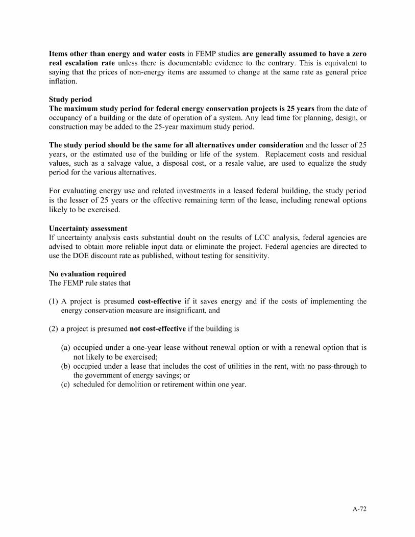
A-72

Items other than energy and water costs in FEMP studies are generally assumed to have a zero real escalation rate unless there is documentable evidence to the contrary. This is equivalent to saying that the prices of non-energy items are assumed to change at the same rate as general price inflation. Study period The maximum study period for federal energy conservation projects is 25 years from the date of occupancy of a building or the date of operation of a system. Any lead time for planning, design, or construction may be added to the 25-year maximum study period. The study period should be the same for all alternatives under consideration and the lesser of 25 years, or the estimated use of the building or life of the system. Replacement costs and residual values, such as a salvage value, a disposal cost, or a resale value, are used to equalize the study period for the various alternatives. For evaluating energy use and related investments in a leased federal building, the study period is the lesser of 25 years or the effective remaining term of the lease, including renewal options likely to be exercised. Uncertainty assessment If uncertainty analysis casts substantial doubt on the results of LCC analysis, federal agencies are advised to obtain more reliable input data or eliminate the project. Federal agencies are directed to use the DOE discount rate as published, without testing for sensitivity. No evaluation required The FEMP rule states that (1) A project is presumed cost-effective if it saves energy and if the costs of implementing the

energy conservation measure are insignificant, and

(2) a project is presumed not cost-effective if the building is

(a) occupied under a one-year lease without renewal option or with a renewal option that is not likely to be exercised;

(b) occupied under a lease that includes the cost of utilities in the rent, with no pass-through to the government of energy savings; or

(c) scheduled for demolition or retirement within one year.

B-1

Module BNIST LCC Software: Overview and BLCC5

• use BLCC5 to evaluate energy and water conservation projects.

• describe the features of other NIST LCC computer programs.

Objectives: Upon completion of this module, you will be able to

B-2

BLCC 5.0-01Building Life-Cycle Cost Program

(windowed version of BLCC4)

for Energy and Water Conservation and Renewable Energy Projects

B-3

Overview - BLCC5• Economic analysis of capital investments that reduce

future costs• Focus on energy and water conservation in buildings• Current modules – agency-funded projects (direct appropriations)– financed projects (ESPC/UC)

• Future modules– MILCON– private sector

• Downloadable from DOE web site

B-4

Data Requirements• Project Information– name, location, analyst, comment, discounting

convention, constant or current dollars, discount rate, base date, service date, and length of study period

• Capital Investment Costs– investment costs– cost-phasing– escalation rates– replacement costs and timing– residual values

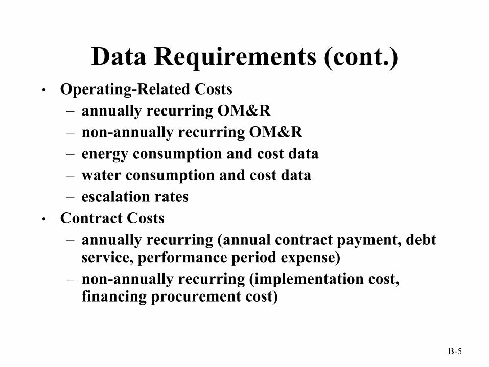
B-5

Data Requirements (cont.)• Operating-Related Costs– annually recurring OM&R– non-annually recurring OM&R– energy consumption and cost data– water consumption and cost data– escalation rates

• Contract Costs– annually recurring (annual contract payment, debt

service, performance period expense)– non-annually recurring (implementation cost,

financing procurement cost)

B-6

Creating a BLCC5 Input File• Input general information for the project.• Input data for each alternative.• Use tree as a guideline and checklist.• Go to Help - Creating and Editing Data Files - for

definitions of all input variables .• Print reports– LCC computations are made each time a report is

opened.• Save project file using user-supplied filename.

B-7

BLCC5 Tree

ProjectAlternative

Component

Cost data

B-8

Project Data

Screen-specific help

B-9

Add/Copy Feature

You can add/copy:

•Alternatives

•Capital Components

•All cost items

B-10

Delete Feature

You can delete:

•Alternatives

•Capital Components

•All cost items

B-11

Energy UsageYou can have usage indices for:

•Energy Costs

•Water Costs

•Annually Recurring Costs

•Annually RecurringContract Costs

B-12

Energy Costs

• Default price escalation rates based on:• rate type• region• fuel typespecified• Rates can be edited.

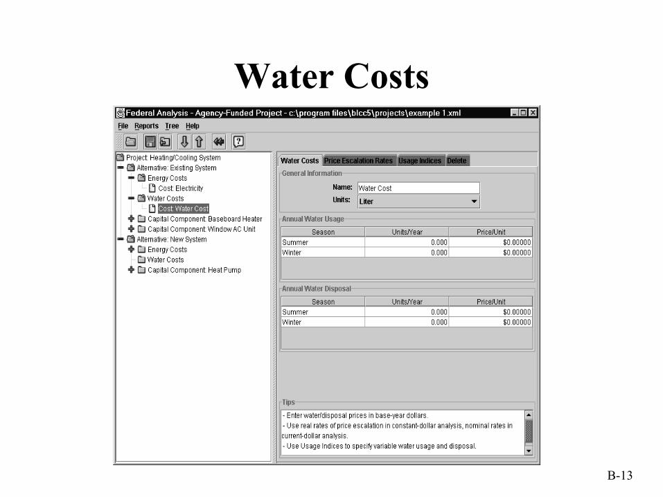
B-13

Water Costs

B-14

Contract CostsAnnually Recurring Non-Annually Recurring

B-15

Investment Costs

Average annual rate of increase during P/C/I period

Investment costs can be phased in over a Planning/Construction or Installation (P/C/I) Period.

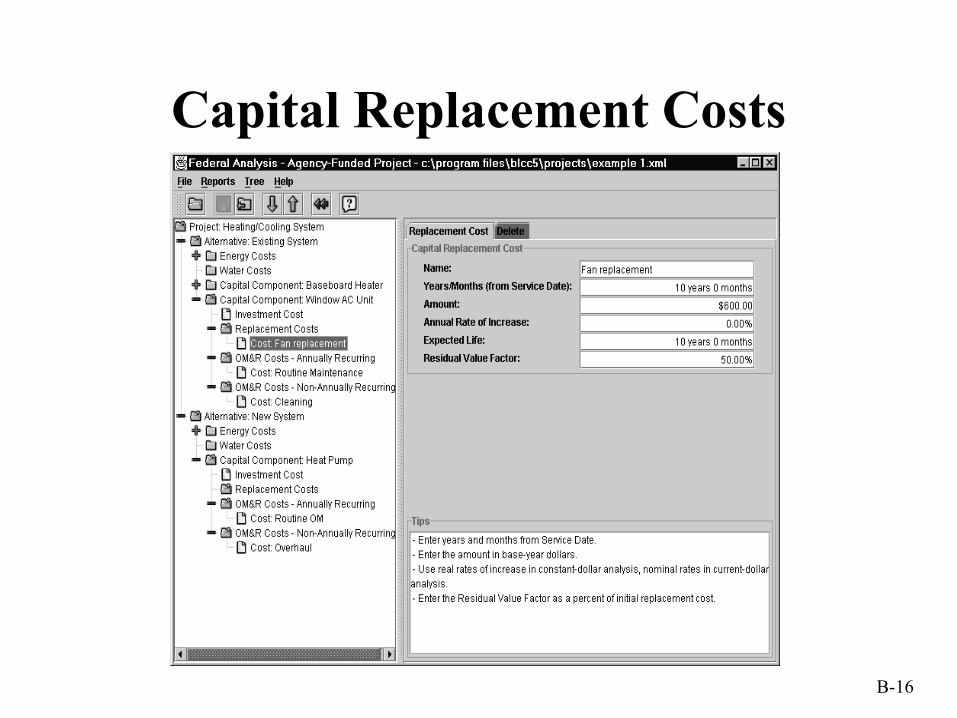
B-16

Capital Replacement Costs

B-17

Operating/Maintenance/Repair Costs

Annually Recurring Non-Annually Recurring

B-18

BLCC5 Reports• For all alternatives in project

– input data listing– life-cycle cost analysis (detailed and summary)– yearly cash flow analysis

• Comparative analysis– listing of LCCs for all project alternatives, with lowest LCC flagged– comparative economic measures (alternative versus base case)– side-by-side comparison of present values – net savings– savings-to-investment ratio– adjusted internal rate of return– payback– energy savings– emission reductions

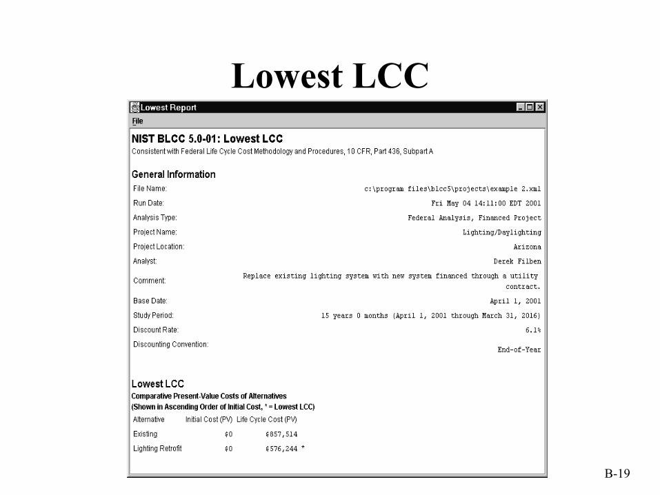
B-19

Lowest LCC

B-20

NIST DOS-Based LCC Support Software

• BLCC4

• ERATES: complex electricity rate schedules

• EMISS: air pollution emission factors

• DISCOUNT: present value factors and calculations

B-21

NIST LCC Programs• Programs updated every April 1 with new energy price

escalation and discount rates

• Downloadable from DOE/FEMP Web site:– www.eren.doe.gov/femp -- Technical Assistance –

Analytical Software Tools

C-1

Module C

Fuel Switching and Phased-In Capital Replacements

Objective: Upon completion of this module, you will be able to

• evaluate capital replacements affecting energy types and energy usage amounts after occupancy.

C-2

Boiler Replacement ProblemLocation: Office building in MarylandExisting: 3 -700 kBtu oil-fired boilers

60% efficient, 15-year remaining life oil price $1.20/gallon ($8.57 MBtu)

Proposal: 3 -700 kBtu gas/oil-fired boilers $15,000 each (installed) 80/83% efficient, 30-year expected life gas price $1.00/therm ($10.00 MBtu)

Maintenance similar for both systemsAnnual heat load = 2,065 MBtuStudy period = 15 yearsFEMP LCC discount rate = 3.3%

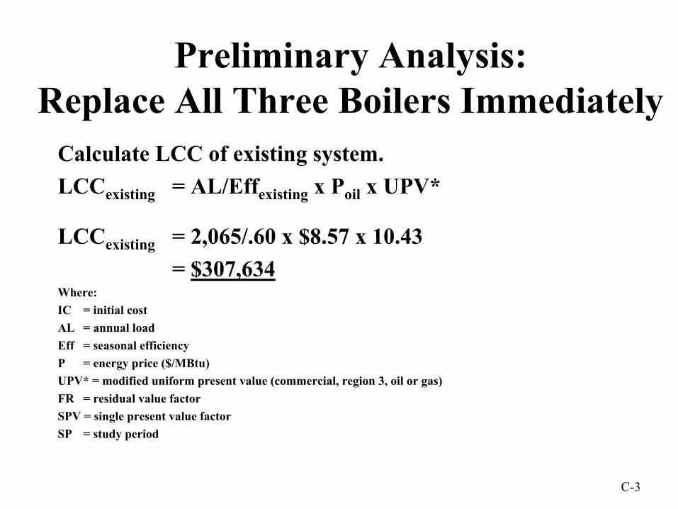
C-3

Preliminary Analysis: Replace All Three Boilers Immediately

Calculate LCC of existing system.LCCexisting = AL/Effexisting x Poil x UPV*

LCCexisting = 2,065/.60 x $8.57 x 10.43= $307,634

Where:IC = initial costAL = annual loadEff = seasonal efficiencyP = energy price ($/MBtu)UPV* = modified uniform present value (commercial, region 3, oil or gas)FR = residual value factorSPV = single present value factorSP = study period

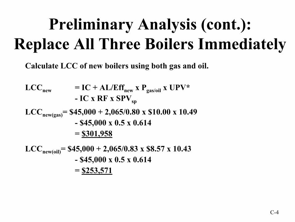
C-4

Preliminary Analysis (cont.): Replace All Three Boilers Immediately

Calculate LCC of new boilers using both gas and oil.

LCCnew = IC + AL/Effnew x Pgas/oil x UPV*- IC x RF x SPVsp

LCCnew(gas)= $45,000 + 2,065/0.80 x $10.00 x 10.49- $45,000 x 0.5 x 0.614= $301,958

LCCnew(oil)= $45,000 + 2,065/0.83 x $8.57 x 10.43- $45,000 x 0.5 x 0.614= $253,571

C-5

Phased-In Boiler ReplacementReplace boiler #1 immediately, #2 at end of year 2, #3 at end of year 4.

LCCnew = IC1 x SPV0 + IC2 x SPV2 + IC3 x SPV4 ++ AL1/Effnew x Poil x UPV*(15,oil,S,com)

+ AL2/Effexisting x Poil x UPV*(2,oil,S,com) + AL2/Effnew x Poil x [UPV*(15,oil,S,com) - UPV*(2,oil,S,com)]

+ AL3/Effexisting x Poil x UPV*(4,oil,S,com) + AL3/Effnew x Poil x [UPV*(15,oil,S,com) - UPV*(4,oil,S,com)]

- IC1 x RF1 x SPV15- IC2 x RF2 x SPV15 - IC3 x RF3 x SPV15

C-6

Boiler Load ProfileThe annual load on each boiler (AL1, AL2, AL3) is needed to

identify energy use as boilers are phased in.

987654321

bin

542018970088932

260070070020007173787007001778125415670070015561713806337001333222540411700111127

744006666683779000444444426840022222247

hrs/ yearboiler 3boiler 2boiler 1

load (kBtu)

outdoor temp

load distribution (kBtu)

C-7

Annual Energy Use by Individual Boiler

41219Total

87654321

bin

4810102379

2,064153451,704

30612128483838184087972820104178

496004963510035115200152

total loadboiler 3boiler 2boiler 1

annual load (MBtu)

C-8

LCC for Existing Boilers

LCC existing(i) = AL1/Effexisting x Poil x UPV*15

LCC existing(1) = 1,704/0.60 x $8.57 x 10.43 = $253,854

LCC existing(2) = 345/0.60 x $8.57 x 10.43 = $51,396

LCC existing(3) = 15/0.60 x $8.57 x 10.43 = $2,235

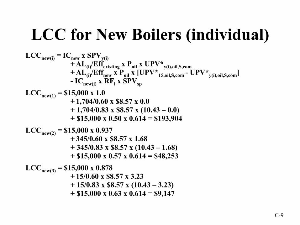
C-9

LCC for New Boilers (individual)LCCnew(i) = ICnew x SPVy(i)

+ AL(i)/Effexisting x Poil x UPV*y(i),oil,S,com+ AL(i)/Effnew x Poil x [UPV*15,oil,S,com - UPV*y(i),oil,S,com]- ICnew(i) x RFi x SPVsp

LCCnew(1) = $15,000 x 1.0+ 1,704/0.60 x $8.57 x 0.0+ 1,704/0.83 x $8.57 x (10.43 – 0.0)+ $15,000 x 0.50 x 0.614 = $193,904

LCCnew(2) = $15,000 x 0.937+ 345/0.60 x $8.57 x 1.68+ 345/0.83 x $8.57 x (10.43 – 1.68)+ $15,000 x 0.57 x 0.614 = $48,253

LCCnew(3) = $15,000 x 0.878+ 15/0.60 x $8.57 x 3.23+ 15/0.83 x $8.57 x (10.43 – 3.23)+ $15,000 x 0.63 x 0.614 = $9,147

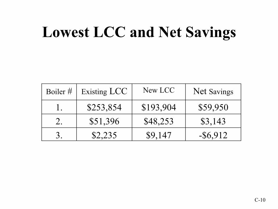
C-10

Lowest LCC and Net Savings

-$6,912$9,147$2,2353.$3,143$48,253$51,3962.$59,950$193,904$253,8541.

Net SavingsNew LCCExisting LCCBoiler #

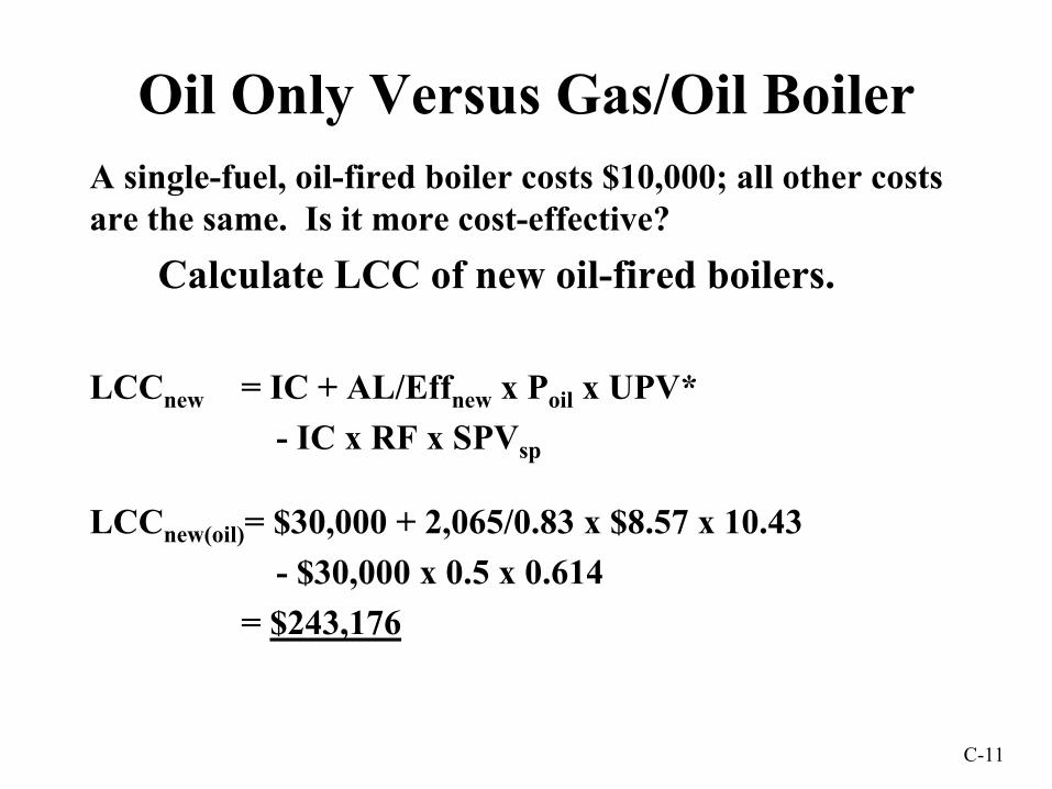
C-11

Oil Only Versus Gas/Oil BoilerA single-fuel, oil-fired boiler costs $10,000; all other costs are the same. Is it more cost-effective?

Calculate LCC of new oil-fired boilers.

LCCnew = IC + AL/Effnew x Poil x UPV*- IC x RF x SPVsp

LCCnew(oil)= $30,000 + 2,065/0.83 x $8.57 x 10.43- $30,000 x 0.5 x 0.614

= $243,176

C-12

Lowest Life-Cycle Cost

$253,571New Gas/Oil-Fired Boiler

$243,176New Oil-Fired Boiler

$307,634Existing Oil-Fired BoilerLCCOption

What other issues need enter into the decision other than lowest LCC?

C-13

Exercise C1Determine the LCC, using BLCC5, for the following three cases:Location: Office building in MarylandAnnual heat load: 2,065 MBtuStudy period: 15 yearsFEMP discount rate: 3.3%Oil price: $1.20/gallon, 140,000 Btu/gallon Gas price: $1.00/therm, 100,000 Btu/thermMaintenance similar for all options.

C-14

Exercise C1 (cont.)

Case 1: Existing 3 - 700 kBtu oil-fired boilers 60% efficient, 15-year remaining life

Case 2: New 3 - 700 kBtu gas/oil-fired boilers $15,000 each, 80/83% (gas/oil) efficient 30-year expected life, fired-on oil

Case 3: New 3 - 700 kBtu gas/oil-fired boilers $15,000 each, 80/83% (gas/oil) efficient30-year expected life, fired-on gas

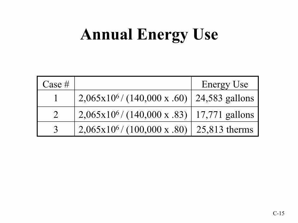
C-15

Annual Energy Use

25,813 therms2,065x106 / (100,000 x .80)317,771 gallons2,065x106 / (140,000 x .83)2

24,583 gallons2,065x106 / (140,000 x .60)1Energy UseCase #

C-16

Alternative 1 – Existing Oil-Fired Boilers

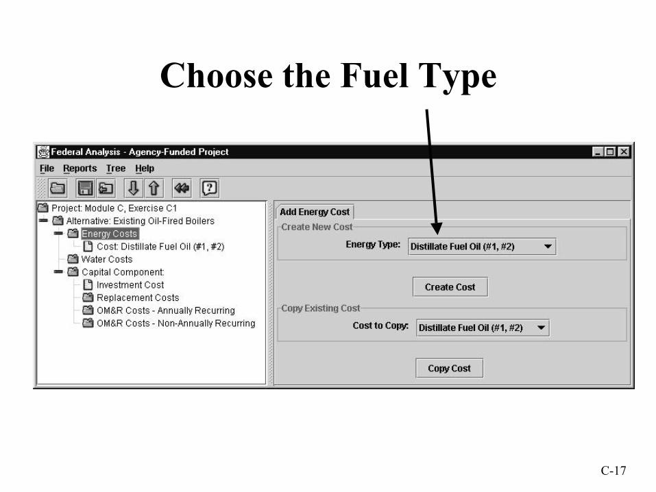
C-17

Choose the Fuel Type

C-18

Enter the Annual Consumption

You can index the use here if needed.

C-19

Enter the Fuel Price and Escalation Information

C-20

Review the Summary LCC Report

C-21

Alternative 2 – Gas/Oil Boilers Burning Oil, Created by Copying Alternative 1

C-22

Enter New Energy Use Data

C-23

Enter Initial Cost, Life, and Residual Value

C-24

Review the Summary LCC Report

C-25

Analyze Alternative 3 and Review Results

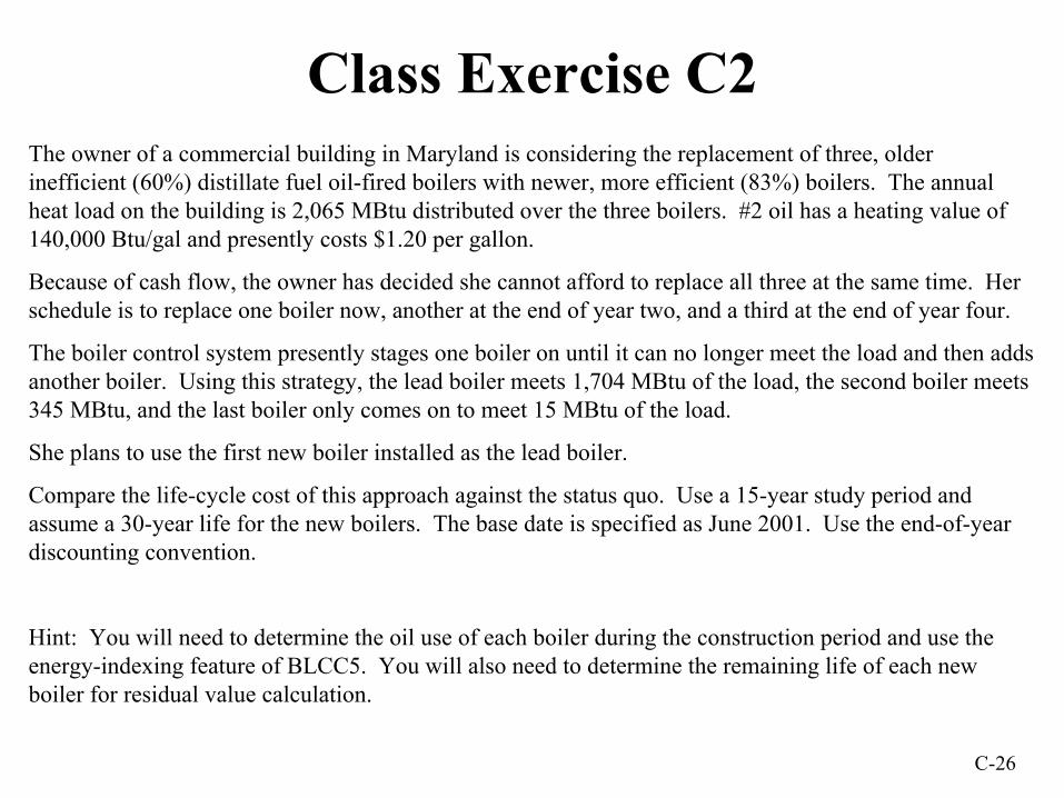
C-26

Class Exercise C2The owner of a commercial building in Maryland is considering the replacement of three, older inefficient (60%) distillate fuel oil-fired boilers with newer, more efficient (83%) boilers. The annual heat load on the building is 2,065 MBtu distributed over the three boilers. #2 oil has a heating value of 140,000 Btu/gal and presently costs $1.20 per gallon.

Because of cash flow, the owner has decided she cannot afford to replace all three at the same time. Her schedule is to replace one boiler now, another at the end of year two, and a third at the end of year four.

The boiler control system presently stages one boiler on until it can no longer meet the load and then adds another boiler. Using this strategy, the lead boiler meets 1,704 MBtu of the load, the second boiler meets 345 MBtu, and the last boiler only comes on to meet 15 MBtu of the load.

She plans to use the first new boiler installed as the lead boiler.

Compare the life-cycle cost of this approach against the status quo. Use a 15-year study period and assume a 30-year life for the new boilers. The base date is specified as June 2001. Use the end-of-year discounting convention.

Hint: You will need to determine the oil use of each boiler during the construction period and use the energy-indexing feature of BLCC5. You will also need to determine the remaining life of each new boiler for residual value calculation.

C-27

Class Exercise C2 (cont.)

Boiler #

Annual Load MBtu

Fuel Used Gallons Year 1 Year 2 Year 3 Year 4

Year 5 through 15

1 old 1,704 20,286 2 old 345 4,107 4,107 4,107 3 old 15 179 179 179 179 179

Total = 24,571 1 new 1,704 14,664 14,664 14,664 14,664 14,664 14,664 2 new 345 2,969 2,969 2,969 2,969 3 new 15 129 129

Total = 17,762 18,950 18,950 17,812 17,812 17,762 Fraction 1 1 0.940 0.940 0.937

Boiler Life Used Life Left Residual Value

Factor

1 15 15 0.502 13 17 0.573 11 19 0.63

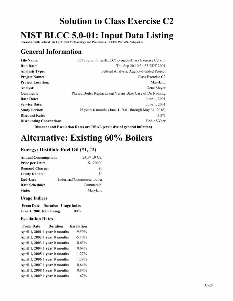
C-28

Solution to Class Exercise C2 NIST BLCC 5.0-01: Input Data Listing Consistent with Federal Life Cycle Cost Methodology and Procedures, 10 CFR, Part 436, Subpart A

General Information File Name: C:\Program Files\BLCC5\projects\Class Exercise C2.xml Run Date: Thu Sep 20 10:34:35 EDT 2001 Analysis Type: Federal Analysis, Agency-Funded Project Project Name: Class Exercise C2 Project Location: Maryland Analyst: Gene Meyer Comment: Phased Boiler Replacement Versus Base Case of Do Nothing Base Date: June 1, 2001 Service Date: June 1, 2001 Study Period: 15 years 0 months (June 1, 2001 through May 31, 2016) Discount Rate: 3.3% Discounting Convention: End-of-Year

Discount and Escalation Rates are REAL (exclusive of general inflation)

Alternative: Existing 60% Boilers Energy: Distillate Fuel Oil (#1, #2) Annual Consumption: 24,571.0 Gal Price per Unit: $1.20000 Demand Charge: $0 Utility Rebate: $0 End-Use: Industrial/Commercial boiler Rate Schedule: Commercial State: Maryland

Usage Indices From Date Duration Usage Index

June 1, 2001 Remaining 100%

Escalation Rates From Date Duration Escalation

April 1, 2001 1 year 0 months -9.59% April 1, 2002 1 year 0 months -5.10% April 1, 2003 1 year 0 months 0.65% April 1, 2004 1 year 0 months 0.64% April 1, 2005 1 year 0 months -1.27% April 1, 2006 1 year 0 months 1.29% April 1, 2007 1 year 0 months 0.64% April 1, 2008 1 year 0 months 0.84% April 1, 2009 1 year 0 months 1.67%

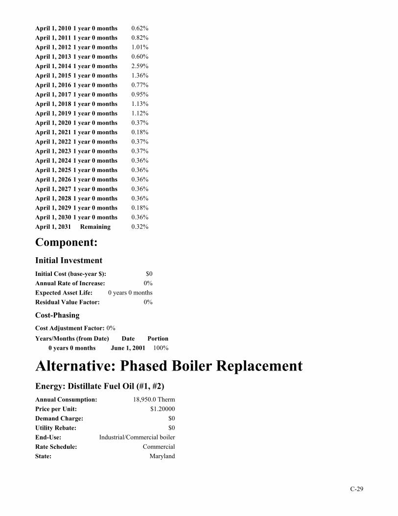
C-29

April 1, 2010 1 year 0 months 0.62% April 1, 2011 1 year 0 months 0.82% April 1, 2012 1 year 0 months 1.01% April 1, 2013 1 year 0 months 0.60% April 1, 2014 1 year 0 months 2.59% April 1, 2015 1 year 0 months 1.36% April 1, 2016 1 year 0 months 0.77% April 1, 2017 1 year 0 months 0.95% April 1, 2018 1 year 0 months 1.13% April 1, 2019 1 year 0 months 1.12% April 1, 2020 1 year 0 months 0.37% April 1, 2021 1 year 0 months 0.18% April 1, 2022 1 year 0 months 0.37% April 1, 2023 1 year 0 months 0.37% April 1, 2024 1 year 0 months 0.36% April 1, 2025 1 year 0 months 0.36% April 1, 2026 1 year 0 months 0.36% April 1, 2027 1 year 0 months 0.36% April 1, 2028 1 year 0 months 0.36% April 1, 2029 1 year 0 months 0.18% April 1, 2030 1 year 0 months 0.36% April 1, 2031 Remaining 0.32%

Component: Initial Investment Initial Cost (base-year $): $0 Annual Rate of Increase: 0% Expected Asset Life: 0 years 0 months Residual Value Factor: 0%

Cost-Phasing Cost Adjustment Factor: 0% Years/Months (from Date) Date Portion

0 years 0 months June 1, 2001 100%

Alternative: Phased Boiler Replacement Energy: Distillate Fuel Oil (#1, #2) Annual Consumption: 18,950.0 Therm Price per Unit: $1.20000 Demand Charge: $0 Utility Rebate: $0 End-Use: Industrial/Commercial boiler Rate Schedule: Commercial State: Maryland

C-30

Usage Indices From Date Duration Usage Index

June 1, 2001 2 years 0 months 100% June 1, 2003 2 years 0 months 94% June 1, 2005 Remaining 93.7%

Escalation Rates From Date Duration Escalation

April 1, 2001 1 year 0 months -9.59% April 1, 2002 1 year 0 months -5.10% April 1, 2003 1 year 0 months 0.65% April 1, 2004 1 year 0 months 0.64% April 1, 2005 1 year 0 months -1.27% April 1, 2006 1 year 0 months 1.29% April 1, 2007 1 year 0 months 0.64% April 1, 2008 1 year 0 months 0.84% April 1, 2009 1 year 0 months 1.67% April 1, 2010 1 year 0 months 0.62% April 1, 2011 1 year 0 months 0.82% April 1, 2012 1 year 0 months 1.01% April 1, 2013 1 year 0 months 0.60% April 1, 2014 1 year 0 months 2.59% April 1, 2015 1 year 0 months 1.36% April 1, 2016 1 year 0 months 0.77% April 1, 2017 1 year 0 months 0.95% April 1, 2018 1 year 0 months 1.13% April 1, 2019 1 year 0 months 1.12% April 1, 2020 1 year 0 months 0.37% April 1, 2021 1 year 0 months 0.18% April 1, 2022 1 year 0 months 0.37% April 1, 2023 1 year 0 months 0.37% April 1, 2024 1 year 0 months 0.36% April 1, 2025 1 year 0 months 0.36% April 1, 2026 1 year 0 months 0.36% April 1, 2027 1 year 0 months 0.36% April 1, 2028 1 year 0 months 0.36% April 1, 2029 1 year 0 months 0.18% April 1, 2030 1 year 0 months 0.36% April 1, 2031 Remaining 0.32%

Component: Boiler #1 Comment: Installed in year 1

Initial Investment Initial Cost (base-year $): $15,000 Annual Rate of Increase: 0% Expected Asset Life: 30 years 0 months Residual Value Factor: 50%

C-31

Cost-Phasing Cost Adjustment Factor: 0% Years/Months (from Date) Date Portion

0 years 0 months June 1, 2001 100%

Component: Boiler #2 Comment: Installed at end of year two.

Initial Investment Initial Cost (base-year $): $15,000 Annual Rate of Increase: 0% Expected Asset Life: 32 years 0 months Residual Value Factor: 57%

Cost-Phasing Cost Adjustment Factor: 0% Years/Months (from Date) Date Portion

2 years 0 months June 1, 2003 100%

Component: Boiler #3 Comment: Installed at end of year 4

Initial Investment Initial Cost (base-year $): $15,000 Annual Rate of Increase: 0% Expected Asset Life: 34 years 0 months Residual Value Factor: 63%

Cost-Phasing Cost Adjustment Factor: 0% Years/Months (from Date) Date Portion

4 years 0 months June 1, 2005 100%

C-32

NIST BLCC 5.0-01: Comparative Analysis Consistent with Federal Life Cycle Cost Methodology and Procedures, 10 CFR, Part 436, Subpart A

Base Case: Existing 60% Boilers Alternative: Phased Boiler Replacement

General Information File Name: C:\Program Files\BLCC5\projects\Class Exercise C2.xml

Run Date: Thu Sep 20 10:44:20 EDT 2001

Project Name: Class Exercise C2

Project Location: Maryland

Analysis Type: Federal Analysis, Agency-Funded Project

Analyst: Gene Meyer

Comment Phased Boiler Replacement Versus Base Case of Do Nothing

Base Date of Study: June 1, 2001

Service Date: June 1, 2001

Study Period: 15 years 0 months(June 1, 2001 through May 31, 2016)

Discount Rate: 3.3%

Discounting Convention: End-of-Year

Comparison of Present-Value Costs PV Life-Cycle Cost Base Case Alternative Savings from Alternative

Initial Investment Costs: Capital Requirements as of Base Date $0 $42,231 -$42,231 Future Costs: Energy Consumption Costs $312,870 $228,639 $84,231 Energy Demand Charges $0 $0 $0 Energy Utility Rebates $0 $0 $0 Water Costs $0 $0 $0 Recurring and Non-Recurring OM&R Costs $0 $0 $0 Capital Replacements $0 $0 $0 Residual Value at End of Study Period $0 -$15,670 $15,670

------------ ------------ ------------ Subtotal (for Future Cost Items) $312,870 $212,969 $99,901

------------ ------------ ------------ Total PV Life-Cycle Cost $312,870 $255,200 $57,670

C-33

Net Savings from Alternative Compared with Base Case PV of Non-Investment Savings $84,231 - Increased Total Investment $26,561

------------ Net Savings $57,670

Savings-to-Investment Ratio (SIR) SIR = 3.17

Adjusted Internal Rate of Return AIRR = 11.56%

Payback Period Estimated Years to Payback (from beginning of Service Period) Simple Payback occurs in year 7 Discounted Payback occurs in year 8

Energy Savings Summary Energy Savings Summary (in stated units) Units are not the same for each energy type; can't report energy savings.

Energy Savings Summary (in MBtu) Energy -----Average Annual Consumption----- Life-Cycle Type Base Case Alternative Savings Savings Distillate Fuel Oil (#1, #2) 3,729.1 MBtu 1,792.3 MBtu 1,936.8 MBtu 29,047.7 MBtu

Emissions Reduction Summary Energy -----Average Annual Emissions----- Life-Cycle Type Base Case Alternative Reduction Reduction Distillate Fuel Oil (#1, #2)

CO2 270,643.67 kg 130,079.04 kg 140,564.63 kg 2,108,180.79 kg SO2 1,935.98 kg 930.49 kg 1,005.49 kg 15,080.33 kg NOx 243.96 kg 117.26 kg 126.71 kg 1,900.37 kg

Total: CO2 270,643.67 kg 130,079.04 kg 140,564.63 kg 2,108,180.79 kg SO2 1,935.98 kg 930.49 kg 1,005.49 kg 15,080.33 kg NOx 243.96 kg 117.26 kg 126.71 kg 1,900.37 kg

D-1

Module DReplacement of Functional Systems

to Improve Energy Efficiency

• cost-effectiveness requirements for– new systems or mandatory replacement of

functional systems– optional replacement of functional systems.

• timing of optional system replacement.• sensitivity analysis.

Objectives: Upon completion of this module, you will understand

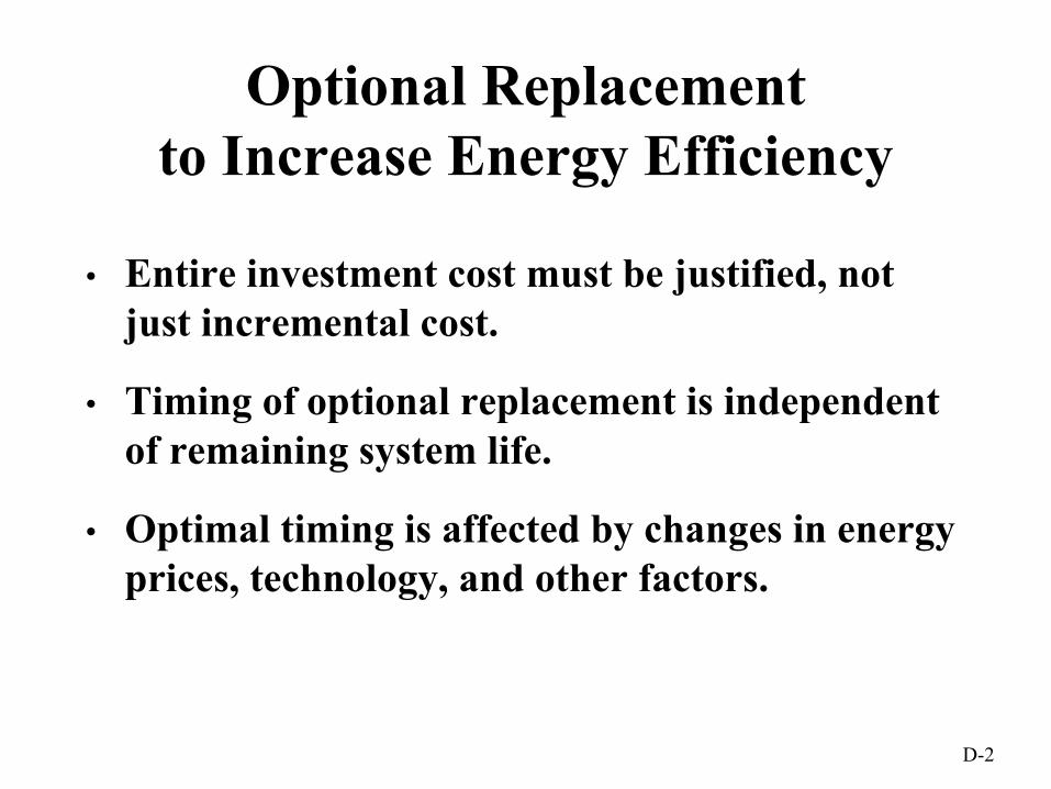
D-2

Optional Replacement to Increase Energy Efficiency

• Entire investment cost must be justified, not just incremental cost.

• Timing of optional replacement is independent of remaining system life.

• Optimal timing is affected by changes in energy prices, technology, and other factors.

D-3

PROBLEM STATEMENT

The existing facility, an 8100 sq. ft. government office building in Virginia, provides administrative space, counseling rooms, and records and research areas. Over time, the increased use of devices such as individual work stations and printers has increased the cooling requirements at the building. The building is currently cooled by several window air conditioners, which require frequent maintenance and consume excessive amounts of energy. On very hot days there are complaints about uncomfortably high temperatures in the building. The building is heated by electric baseboard heating.

OptionsMaintain Existing SystemWith the current maintenance schedule, the present heating and cooling system could be kept functional for another 20 years.

Install DX Split SystemInstall new “split-system” air-conditioning unit and associated elements required to provide adequate space conditioning. The installation will provide a new air distribution system for the building, with central air conditioning throughout.

Connect to Central Chilled Water PlantInstall piping network to connect the office building to the central chilled water plant on the site. The installation will provide a new air distribution system for the building, with air conditioning throughout. This option, if cost-effective, would be preferred to the DX Split System because it would allow centralized maintenance. A general overhaul of the Central Plant is scheduled for 2004. If the piping connection to the office building were done then, the initial investment cost would be reduced by about 15%.

Electric baseboard heating will continue to be used for the facility. The removed air conditioning units will not have any appreciable salvage value. Either upgrade will require a planning and installation period of one year. The equipment installation will inconvenience personnel in the office building but should not shut the office down

Exercise D1Economic Evaluation of Air Conditioning System

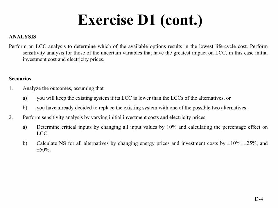
D-4

Exercise D1 (cont.)ANALYSIS

Perform an LCC analysis to determine which of the available options results in the lowest life-cycle cost. Perform sensitivity analysis for those of the uncertain variables that have the greatest impact on LCC, in this case initial investment cost and electricity prices.

Scenarios

1. Analyze the outcomes, assuming that

a) you will keep the existing system if its LCC is lower than the LCCs of the alternatives, or

b) you have already decided to replace the existing system with one of the possible two alternatives.

2. Perform sensitivity analysis by varying initial investment costs and electricity prices.

a) Determine critical inputs by changing all input values by 10% and calculating the percentage effect on LCC.

b) Calculate NS for all alternatives by changing energy prices and investment costs by ±10%, ±25%, and ±50%.

D-5

• AC system in NAVFAC office building in Virginia

• Discount rate: 3.3%

• Mid-year discounting

• Constant-dollar analysis

• Agency-funded project

General Project Information

D-6

Key dates

• Base Date: June 2001• Study period: 21 years • Implementation Period: 1 year• Service Date: June 2002

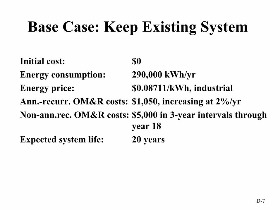
D-7

Base Case: Keep Existing System

Initial cost: $0Energy consumption: 290,000 kWh/yrEnergy price: $0.08711/kWh, industrialAnn.-recurr. OM&R costs: $1,050, increasing at 2%/yrNon-ann.rec. OM&R costs: $5,000 in 3-year intervals through

year 18Expected system life: 20 years

D-8

Alternative I: DX Split System AC

Initial cost: $210,000Energy consumption: 120,330 kWh/yrEnergy price: $0.08711/kWh, industrialAnn.-recurr. OM&R costs: $530Non-ann.rec. OM&R costs: $6,300 in yrs. 5, 10, 15Capital replacement cost: $31,130 in year 15

Useful Life: 15 yearsResidual Value Factor: 67%

Expected system life: 20 years

D-9

Alternative II: Central Plant Connection

Initial cost: $265,000Energy consumption: 112,000 kWh/yrEnergy price: $0.08711/kWh, industrialAnn.-recurr. OM&R costs: $126Non-ann.rec. OM&R costs: $950 in yrs 3, 9, 15, 18Expected system life: 20 years

D-10

DX Split System - Cash Flow Diagram

01 02 03 04 05 06 07 08 09 10 11 12 … 17 18 19 20 21

BD SD

Energy, OM&R

Inv.Rep. Rep. Rep.

Replacement

Residual Value

D-11

Key DatesImplementation Period

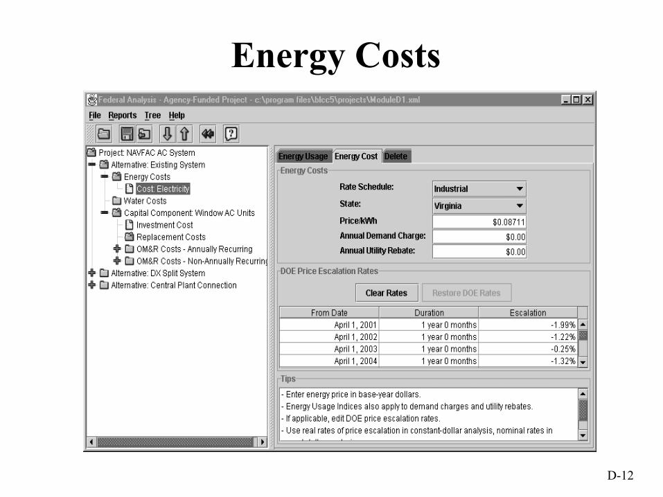
D-12

Energy Costs

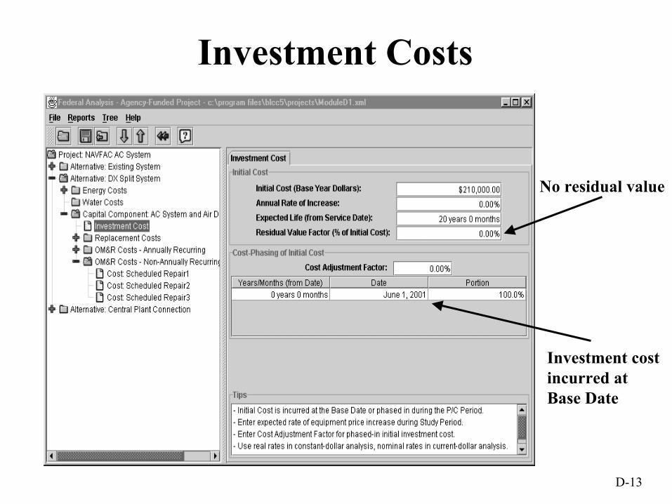
D-13

Investment Costs

Investment costincurred atBase Date

No residual value

D-14

OM&R Costs

NAR repairs in yrs. 5,10,15

D-15

Lowest LCCExisting System

D-16

Ex. S. DX SS

Total investment > savings

Existing System and DX SS

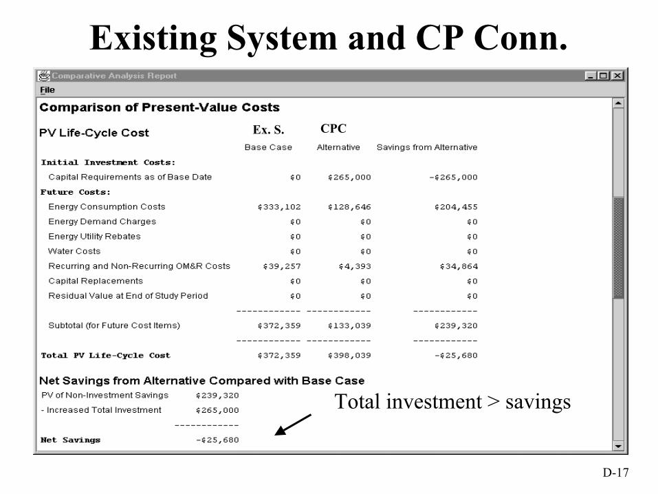
D-17

Existing System and CP Conn.

Total investment > savings

Ex. S. CPC

D-18

LCCs - Optional ReplacementFor optional replacement of a functional system,

entire investment cost must be supported by savings.

Base Case Costs Savings from Upgrades Ex. System DX SS CPC

Investment 0 - $210,000 - $265,000Replacement costs - - 18,517 -Residual Value - 10,549 -

Total Inv. Costs -$217,969 -$265,000PV energy costs $333,102 194,887 204,456PV OM&R costs 39,257 18,369 34,864Total Operat’l Costs $213,257 $239,320Net Savings - -$ 4,712 -$ 25,680

D-19

DX Split System and Central Plant Conn.

DX SS CPC

Incremental investment costs

D-20

LCCs - Mandatory ReplacementFor new system or mandatory replacement of an existing system,

incremental investment cost must be supported by savings.

Costs SavingsDX SS CPC from alternative

Investment $210,000 $265,000 -$ 55,000 Replacement costs 18,517 - 18,517Residual Value -10,549 - - 10,549

Total Inv. Costs $217,968 $265,000 -$47,032PV energy costs 138,214 134,141 9,568PV OM&R costs 20,888 4,393 16,495Total Operat’l Costs $159,102 $138,534 $ 26,063Net Savings - -$ 20,969

D-21

LCCs of AC Systems (cont.)Analysis results:

• If replacement is optional, Existing System has lowest LCC.• If replacement is mandatory, DX Split System has lowest LCC. • Central Plant Connection is not cost-effective in either case.

Other considerations:• Outcome may be changed by

– Change in energy prices, investment or OM&R costs.– Change in heating and cooling requirements, timing, and other

factors.Evaluate other option:

• Postpone Central Plant Connection.

D-22

Sensitivity Analysis

Repeat economic evaluation with one or more input values changed.

• Determine– which input values are uncertain.– which input values are critical.

• Evaluate – effect of changes on LCC, NS, or any

other measure of economic evaluation.

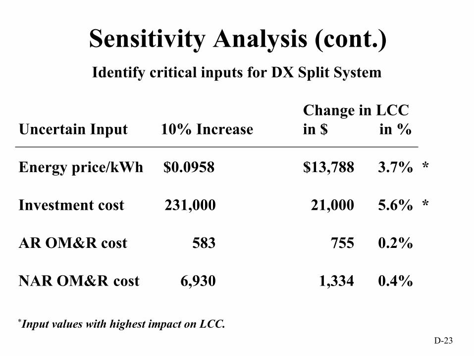
D-23

Sensitivity Analysis (cont.)Identify critical inputs for DX Split System

Change in LCCUncertain Input 10% Increase in $ in %

Energy price/kWh $0.0958 $13,788 3.7% *

Investment cost 231,000 21,000 5.6% *

AR OM&R cost 583 755 0.2%

NAR OM&R cost 6,930 1,334 0.4%

*Input values with highest impact on LCC.

D-24

Sensitivity Analysis (cont.)Sensitivity of Net Savings to Investment Costs

-300,000

-200,000

-100,000

0

100,000

200,000

300,000

-50 -25 -10 0 +10 +25 +50Percent Change

Net

Sav

ings

($)

Central Plant ConnectionDX Split SystemExisting System

D-25

Sensitivity Analysis (cont.)Sensitivity of Net Savings to Electricity Price

-150,000

-100,000

-50,000

0

50,000

100,000

150,000

-50 -25 -10 0 +10 +25 +50

Percent Change

PV

Net

Sav

ings

($)

Central Plant Conn.DX Split SystemExisting System

D-26

Postponed Central Plant Connection

Postpone CP Connection by three years- Use cost phasing of initial investment cost.- Use residual value factor of 15%. - Use indexing to postpone energy and OM&R costs.- Include energy costs and OM&R costs of the

existing system for the three-year delay.Perform Sensitivity Analysis- Increase electricity costs for DX Split System by

35%.

D-27

PP CP Conn. - Cash Flow Diagram

01 02 03 04 05 06 07 08 09 ... 14 15 16 17 18 19 20 21

BD

Energy, OM&R

Inv. Rep. Rep.

Residual Value

SD1

existing system

PP CP Conn.

Rep.SD2

D-28

Cost Phasing of Initial InvestmentPostpone Initial Investment Cost by three years

D-29

Indexing of Energy Usage

Adjustenergyusage

D-30

Indexing of OM&R Costs

AdjustOM&Rusage

D-31

Lowest LCC Report

**

Lowest LCC:Postp. Centr. Plant Conn.

D-32

DX SS and Postponed CP Conn.

PP CPCDX Sp. Sys.

Positive Net Savings

D-33

Hi-E SS and Imm. CP Conn.

ImmediateCP Conn.

Hi-E. DX SS

Lower Life-Cycle Cost

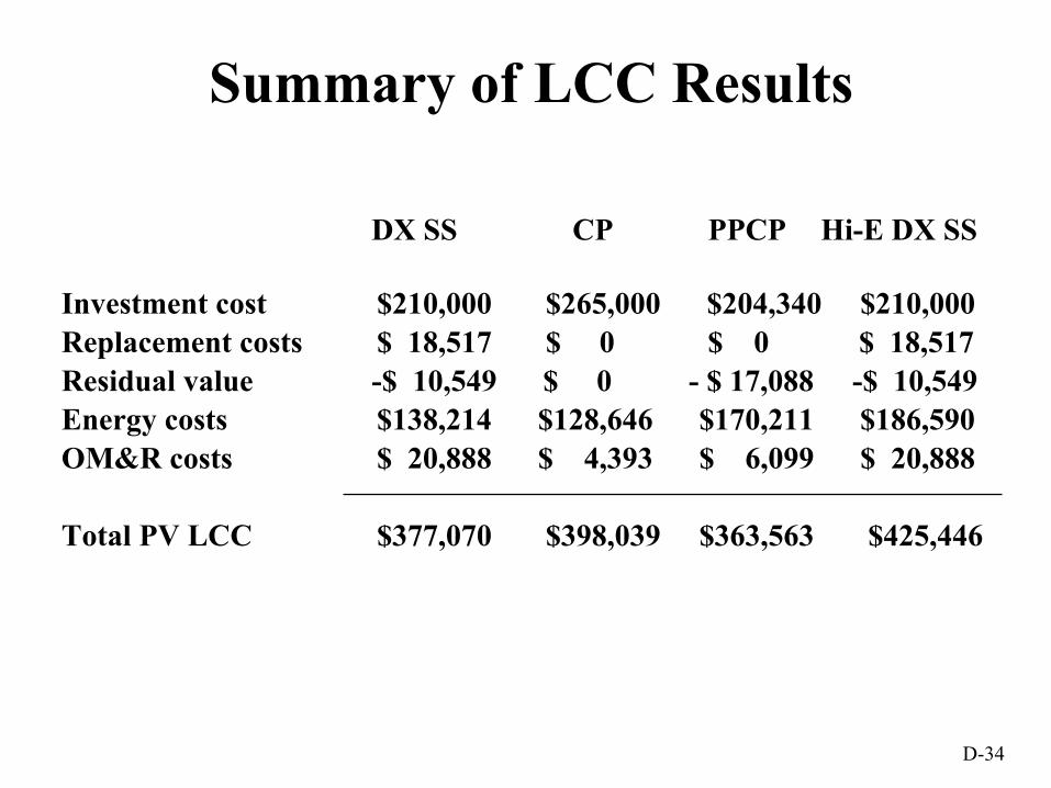
D-34

Summary of LCC Results

DX SS CP PPCP Hi-E DX SS

Investment cost $210,000 $265,000 $204,340 $210,000 Replacement costs $ 18,517 $ 0 $ 0 $ 18,517 Residual value -$ 10,549 $ 0 - $ 17,088 -$ 10,549Energy costs $138,214 $128,646 $170,211 $186,590OM&R costs $ 20,888 $ 4,393 $ 6,099 $ 20,888

Total PV LCC $377,070 $398,039 $363,563 $425,446

D-35

Comparison of LCC Costs

$372.4 $377.1K $363.5K$398.0K

$425.4K

Ex.S SS CP PP CP Hi-E SS

D-36

Summary of Analysis Results• Cost-effectiveness selection depends on circumstances

and timing. • Other considerations:

– Postponed CP Connection has higher life-cycle energy consumption and emissions than immediate installation of DX Split System.

– LCC for postponed CP Connection does not include productivity losses for period of delay.

• Conclusion:– Lowest LCC is one among many criteria that affect

decision making.

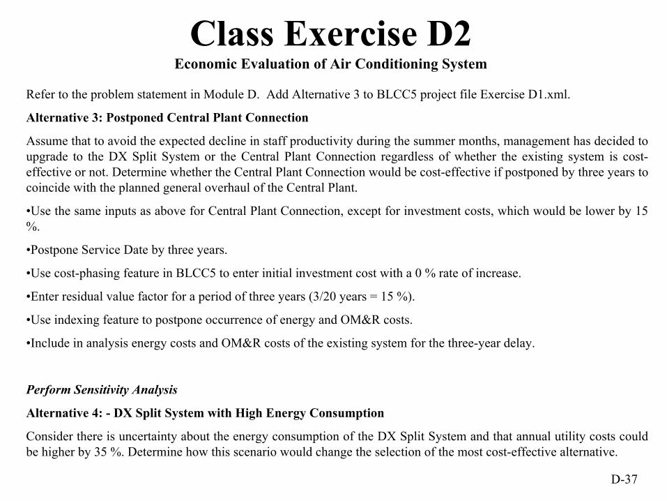
D-37

Class Exercise D2Economic Evaluation of Air Conditioning System

Refer to the problem statement in Module D. Add Alternative 3 to BLCC5 project file Exercise D1.xml.

Alternative 3: Postponed Central Plant Connection

Assume that to avoid the expected decline in staff productivity during the summer months, management has decided toupgrade to the DX Split System or the Central Plant Connection regardless of whether the existing system is cost-effective or not. Determine whether the Central Plant Connection would be cost-effective if postponed by three years tocoincide with the planned general overhaul of the Central Plant.

•Use the same inputs as above for Central Plant Connection, except for investment costs, which would be lower by 15%.

•Postpone Service Date by three years.

•Use cost-phasing feature in BLCC5 to enter initial investment cost with a 0 % rate of increase.

•Enter residual value factor for a period of three years (3/20 years = 15 %).

•Use indexing feature to postpone occurrence of energy and OM&R costs.

•Include in analysis energy costs and OM&R costs of the existing system for the three-year delay.

Perform Sensitivity Analysis

Alternative 4: - DX Split System with High Energy Consumption

Consider there is uncertainty about the energy consumption of the DX Split System and that annual utility costs couldbe higher by 35 %. Determine how this scenario would change the selection of the most cost-effective alternative.

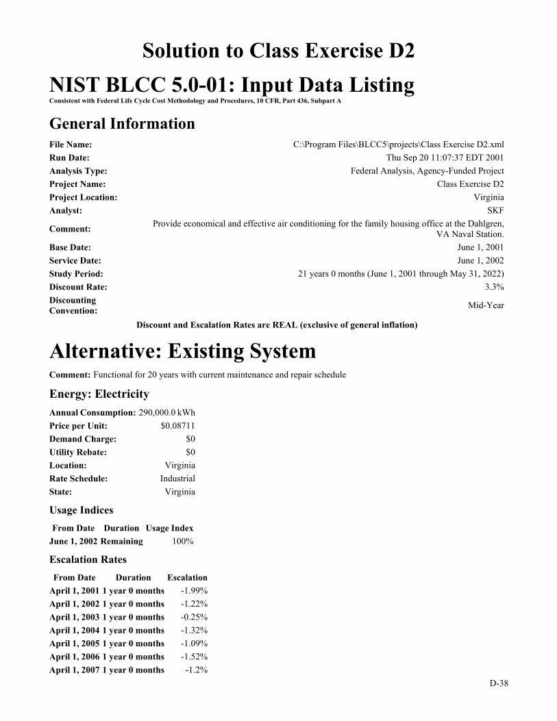
D-38

Solution to Class Exercise D2 NIST BLCC 5.0-01: Input Data Listing Consistent with Federal Life Cycle Cost Methodology and Procedures, 10 CFR, Part 436, Subpart A

General Information File Name: C:\Program Files\BLCC5\projects\Class Exercise D2.xml Run Date: Thu Sep 20 11:07:37 EDT 2001 Analysis Type: Federal Analysis, Agency-Funded Project Project Name: Class Exercise D2 Project Location: Virginia Analyst: SKF

Comment: Provide economical and effective air conditioning for the family housing office at the Dahlgren, VA Naval Station.

Base Date: June 1, 2001 Service Date: June 1, 2002 Study Period: 21 years 0 months (June 1, 2001 through May 31, 2022) Discount Rate: 3.3% Discounting Convention: Mid-Year

Discount and Escalation Rates are REAL (exclusive of general inflation)

Alternative: Existing System Comment: Functional for 20 years with current maintenance and repair schedule

Energy: Electricity Annual Consumption: 290,000.0 kWh Price per Unit: $0.08711 Demand Charge: $0 Utility Rebate: $0 Location: Virginia Rate Schedule: Industrial State: Virginia

Usage Indices From Date Duration Usage Index

June 1, 2002 Remaining 100%

Escalation Rates From Date Duration Escalation

April 1, 2001 1 year 0 months -1.99% April 1, 2002 1 year 0 months -1.22% April 1, 2003 1 year 0 months -0.25% April 1, 2004 1 year 0 months -1.32% April 1, 2005 1 year 0 months -1.09% April 1, 2006 1 year 0 months -1.52% April 1, 2007 1 year 0 months -1.2%

D-39

April 1, 2008 1 year 0 months -0.87% April 1, 2009 1 year 0 months -0.35% April 1, 2010 1 year 0 months -0.79% April 1, 2011 1 year 0 months -0.8% April 1, 2012 1 year 0 months -0.27% April 1, 2013 1 year 0 months 0.36% April 1, 2014 1 year 0 months 0.36% April 1, 2015 1 year 0 months 0.62% April 1, 2016 1 year 0 months 0.79% April 1, 2017 1 year 0 months 0.79% April 1, 2018 1 year 0 months 0.43% April 1, 2019 1 year 0 months 0.61% April 1, 2020 1 year 0 months 0.26% April 1, 2021 1 year 0 months 0.26% April 1, 2022 1 year 0 months 0.26% April 1, 2023 1 year 0 months 0.17% April 1, 2024 1 year 0 months 0.26% April 1, 2025 1 year 0 months 0.25% April 1, 2026 1 year 0 months 0.17% April 1, 2027 1 year 0 months 0.25% April 1, 2028 1 year 0 months 0.25% April 1, 2029 1 year 0 months 0.25% April 1, 2030 1 year 0 months 0.17% April 1, 2031 Remaining 0.22%

Component: Window AC Units Initial Investment Initial Cost (base-year $): $0 Annual Rate of Increase: 0% Expected Asset Life: 20 years 0 months Residual Value Factor: 0%

Cost-Phasing Cost Adjustment Factor: 0% Years/Months (from Date) Date Portion

0 years 0 months June 1, 2001 100%

Recurring OM&R: Routine OM&R Amount: $1,050 Annual Rate of Increase: 2.0%

Usage Indices From Date Duration Factor

June 1, 2002 Remaining 100%

Non-Recurring OM&R: Major Repair1 Years/Months: 3 years 0 months Amount: $5,000

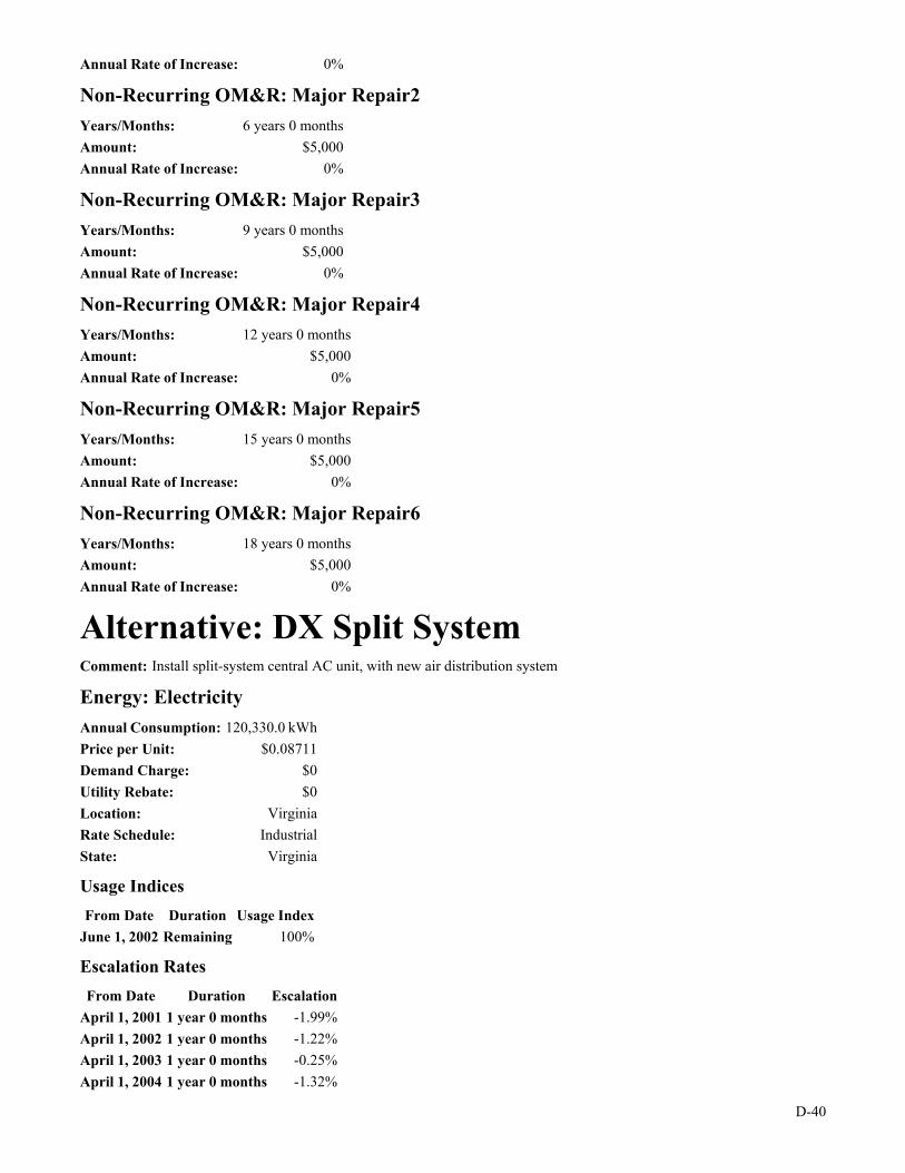
D-40

Annual Rate of Increase: 0%

Non-Recurring OM&R: Major Repair2 Years/Months: 6 years 0 months Amount: $5,000 Annual Rate of Increase: 0%

Non-Recurring OM&R: Major Repair3 Years/Months: 9 years 0 months Amount: $5,000 Annual Rate of Increase: 0%

Non-Recurring OM&R: Major Repair4 Years/Months: 12 years 0 months Amount: $5,000 Annual Rate of Increase: 0%

Non-Recurring OM&R: Major Repair5 Years/Months: 15 years 0 months Amount: $5,000 Annual Rate of Increase: 0%

Non-Recurring OM&R: Major Repair6 Years/Months: 18 years 0 months Amount: $5,000 Annual Rate of Increase: 0%

Alternative: DX Split System Comment: Install split-system central AC unit, with new air distribution system

Energy: Electricity Annual Consumption: 120,330.0 kWh Price per Unit: $0.08711 Demand Charge: $0 Utility Rebate: $0 Location: Virginia Rate Schedule: Industrial State: Virginia

Usage Indices From Date Duration Usage Index

June 1, 2002 Remaining 100%

Escalation Rates From Date Duration Escalation

April 1, 2001 1 year 0 months -1.99% April 1, 2002 1 year 0 months -1.22% April 1, 2003 1 year 0 months -0.25% April 1, 2004 1 year 0 months -1.32%

D-41

April 1, 2005 1 year 0 months -1.09% April 1, 2006 1 year 0 months -1.52% April 1, 2007 1 year 0 months -1.2% April 1, 2008 1 year 0 months -0.87% April 1, 2009 1 year 0 months -0.35% April 1, 2010 1 year 0 months -0.79% April 1, 2011 1 year 0 months -0.8% April 1, 2012 1 year 0 months -0.27% April 1, 2013 1 year 0 months 0.36% April 1, 2014 1 year 0 months 0.36% April 1, 2015 1 year 0 months 0.62% April 1, 2016 1 year 0 months 0.79% April 1, 2017 1 year 0 months 0.79% April 1, 2018 1 year 0 months 0.43% April 1, 2019 1 year 0 months 0.61% April 1, 2020 1 year 0 months 0.26% April 1, 2021 1 year 0 months 0.26% April 1, 2022 1 year 0 months 0.26% April 1, 2023 1 year 0 months 0.17% April 1, 2024 1 year 0 months 0.26% April 1, 2025 1 year 0 months 0.25% April 1, 2026 1 year 0 months 0.17% April 1, 2027 1 year 0 months 0.25% April 1, 2028 1 year 0 months 0.25% April 1, 2029 1 year 0 months 0.25% April 1, 2030 1 year 0 months 0.17% April 1, 2031 Remaining 0.22%

Component: AC System and Air Distribution Initial Investment Initial Cost (base-year $): $210,000 Annual Rate of Increase: 0% Expected Asset Life: 20 years 0 months Residual Value Factor: 0%

Cost-Phasing Cost Adjustment Factor: 0% Years/Months (from Date) Date Portion

0 years 0 months June 1, 2001 100%

Replacement: Compressor/Condens Years/Months: 15 years 0 months Amount: $31,130 Annual Rate Of Increase: 0% Expected Asset Life: 15 years 0 months Residual Value Factor: 67%

D-42

Recurring OM&R: Routine OM&R Amount: $530 Annual Rate of Increase: 0%

Usage Indices From Date Duration Factor

June 1, 2002 Remaining 100%

Non-Recurring OM&R: Scheduled Repair1 Years/Months: 5 years 0 months Amount: $6,300 Annual Rate of Increase: 0%

Non-Recurring OM&R: Scheduled Repair2 Years/Months: 10 years 0 months Amount: $6,300 Annual Rate of Increase: 0%

Non-Recurring OM&R: Scheduled Repair3 Years/Months: 15 years 0 months Amount: $6,300 Annual Rate of Increase: 0%

Alternative: Central Plant Connection Comment: Install piping network to connect officebuilding to central chilled water plant

Energy: Electricity Annual Consumption: 112,000.0 kWh Price per Unit: $0.08711 Demand Charge: $0 Utility Rebate: $0 Location: Virginia Rate Schedule: Industrial State: Virginia

Usage Indices From Date Duration Usage Index

June 1, 2002 Remaining 100%

Escalation Rates From Date Duration Escalation

April 1, 2001 1 year 0 months -1.99% April 1, 2002 1 year 0 months -1.22% April 1, 2003 1 year 0 months -0.25% April 1, 2004 1 year 0 months -1.32% April 1, 2005 1 year 0 months -1.09% April 1, 2006 1 year 0 months -1.52% April 1, 2007 1 year 0 months -1.2% April 1, 2008 1 year 0 months -0.87%

D-43

April 1, 2009 1 year 0 months -0.35% April 1, 2010 1 year 0 months -0.79% April 1, 2011 1 year 0 months -0.8% April 1, 2012 1 year 0 months -0.27% April 1, 2013 1 year 0 months 0.36% April 1, 2014 1 year 0 months 0.36% April 1, 2015 1 year 0 months 0.62% April 1, 2016 1 year 0 months 0.79% April 1, 2017 1 year 0 months 0.79% April 1, 2018 1 year 0 months 0.43% April 1, 2019 1 year 0 months 0.61% April 1, 2020 1 year 0 months 0.26% April 1, 2021 1 year 0 months 0.26% April 1, 2022 1 year 0 months 0.26% April 1, 2023 1 year 0 months 0.17% April 1, 2024 1 year 0 months 0.26% April 1, 2025 1 year 0 months 0.25% April 1, 2026 1 year 0 months 0.17% April 1, 2027 1 year 0 months 0.25% April 1, 2028 1 year 0 months 0.25% April 1, 2029 1 year 0 months 0.25% April 1, 2030 1 year 0 months 0.17% April 1, 2031 Remaining 0.22%

Component: Piping Network and Air Distribution Initial Investment Initial Cost (base-year $): $265,000 Annual Rate of Increase: 0% Expected Asset Life: 20 years 0 months Residual Value Factor: 0%

Cost-Phasing Cost Adjustment Factor: 0% Years/Months (from Date) Date Portion

0 years 0 months June 1, 2001 100%

Recurring OM&R: Routine OM&R Amount: $126 Annual Rate of Increase: 0%

Usage Indices From Date Duration Factor

June 1, 2002 Remaining 100%

Non-Recurring OM&R: Scheduled Repair1 Years/Months: 3 years 0 months Amount: $950 Annual Rate of Increase: 0%

D-44

Non-Recurring OM&R: Scheduled Repair2 Years/Months: 9 years 0 months Amount: $950 Annual Rate of Increase: 0%

Non-Recurring OM&R: Scheduled Repair3 Years/Months: 15 years 0 months Amount: $950 Annual Rate of Increase: 0%

Non-Recurring OM&R: Scheduled Repair1 Years/Months: 18 years 0 months Amount: $950 Annual Rate of Increase: 0%

Alternative: Postponed Central Plant Connection Comment: Postpone installation of piping network to 2004 to coincide with general over- haul of Central Plant. The AC

system would become operational in 2005.

Energy: Electricity - after connection Annual Consumption: 112,000.0 kWh Price per Unit: $0.08711 Demand Charge: $0 Utility Rebate: $0 Location: Virginia Rate Schedule: Industrial State: Virginia

Usage Indices From Date Duration Usage Index

June 1, 2002 3 years 0 months 0% June 1, 2005 Remaining 100%

Escalation Rates From Date Duration Escalation

April 1, 2001 1 year 0 months -1.99% April 1, 2002 1 year 0 months -1.22% April 1, 2003 1 year 0 months -0.25% April 1, 2004 1 year 0 months -1.32% April 1, 2005 1 year 0 months -1.09% April 1, 2006 1 year 0 months -1.52% April 1, 2007 1 year 0 months -1.2% April 1, 2008 1 year 0 months -0.87% April 1, 2009 1 year 0 months -0.35% April 1, 2010 1 year 0 months -0.79% April 1, 2011 1 year 0 months -0.8%

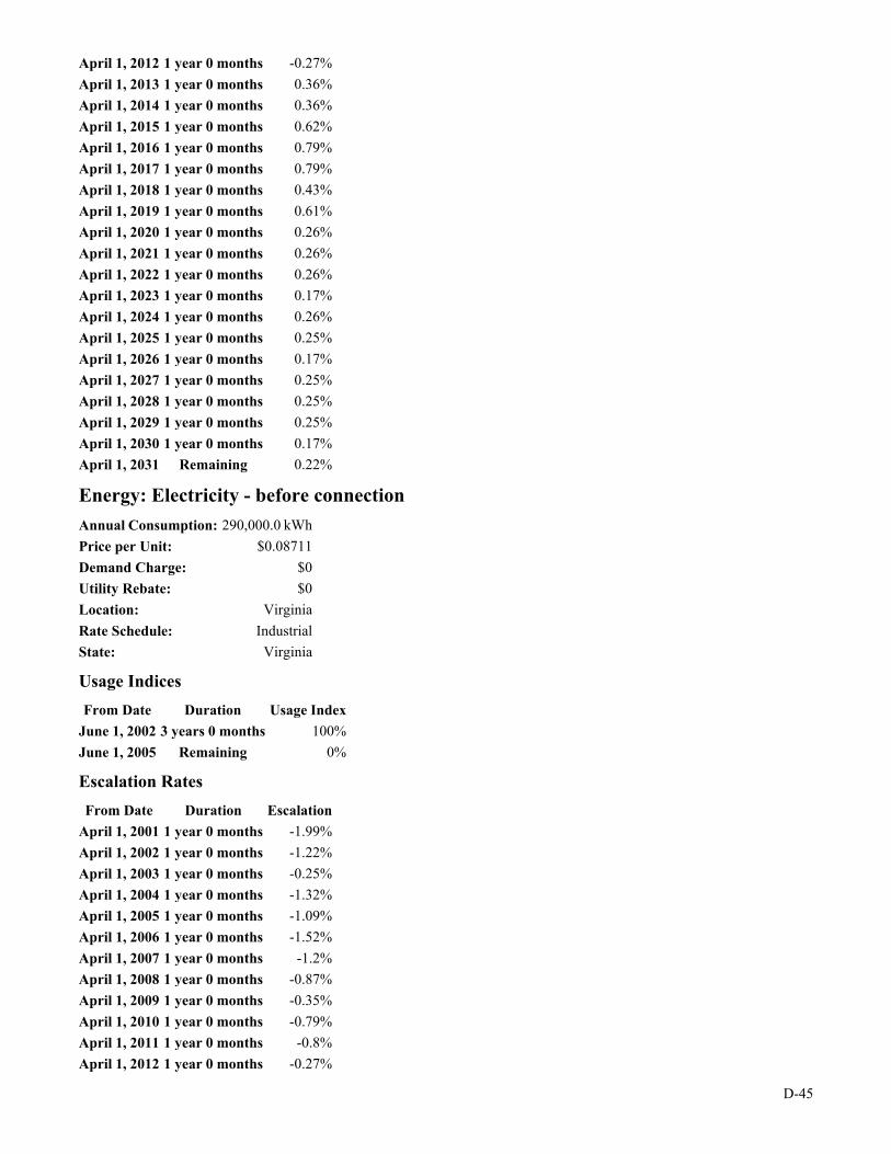
D-45

April 1, 2012 1 year 0 months -0.27% April 1, 2013 1 year 0 months 0.36% April 1, 2014 1 year 0 months 0.36% April 1, 2015 1 year 0 months 0.62% April 1, 2016 1 year 0 months 0.79% April 1, 2017 1 year 0 months 0.79% April 1, 2018 1 year 0 months 0.43% April 1, 2019 1 year 0 months 0.61% April 1, 2020 1 year 0 months 0.26% April 1, 2021 1 year 0 months 0.26% April 1, 2022 1 year 0 months 0.26% April 1, 2023 1 year 0 months 0.17% April 1, 2024 1 year 0 months 0.26% April 1, 2025 1 year 0 months 0.25% April 1, 2026 1 year 0 months 0.17% April 1, 2027 1 year 0 months 0.25% April 1, 2028 1 year 0 months 0.25% April 1, 2029 1 year 0 months 0.25% April 1, 2030 1 year 0 months 0.17% April 1, 2031 Remaining 0.22%

Energy: Electricity - before connection Annual Consumption: 290,000.0 kWh Price per Unit: $0.08711 Demand Charge: $0 Utility Rebate: $0 Location: Virginia Rate Schedule: Industrial State: Virginia

Usage Indices From Date Duration Usage Index

June 1, 2002 3 years 0 months 100% June 1, 2005 Remaining 0%

Escalation Rates From Date Duration Escalation

April 1, 2001 1 year 0 months -1.99% April 1, 2002 1 year 0 months -1.22% April 1, 2003 1 year 0 months -0.25% April 1, 2004 1 year 0 months -1.32% April 1, 2005 1 year 0 months -1.09% April 1, 2006 1 year 0 months -1.52% April 1, 2007 1 year 0 months -1.2% April 1, 2008 1 year 0 months -0.87% April 1, 2009 1 year 0 months -0.35% April 1, 2010 1 year 0 months -0.79% April 1, 2011 1 year 0 months -0.8% April 1, 2012 1 year 0 months -0.27%

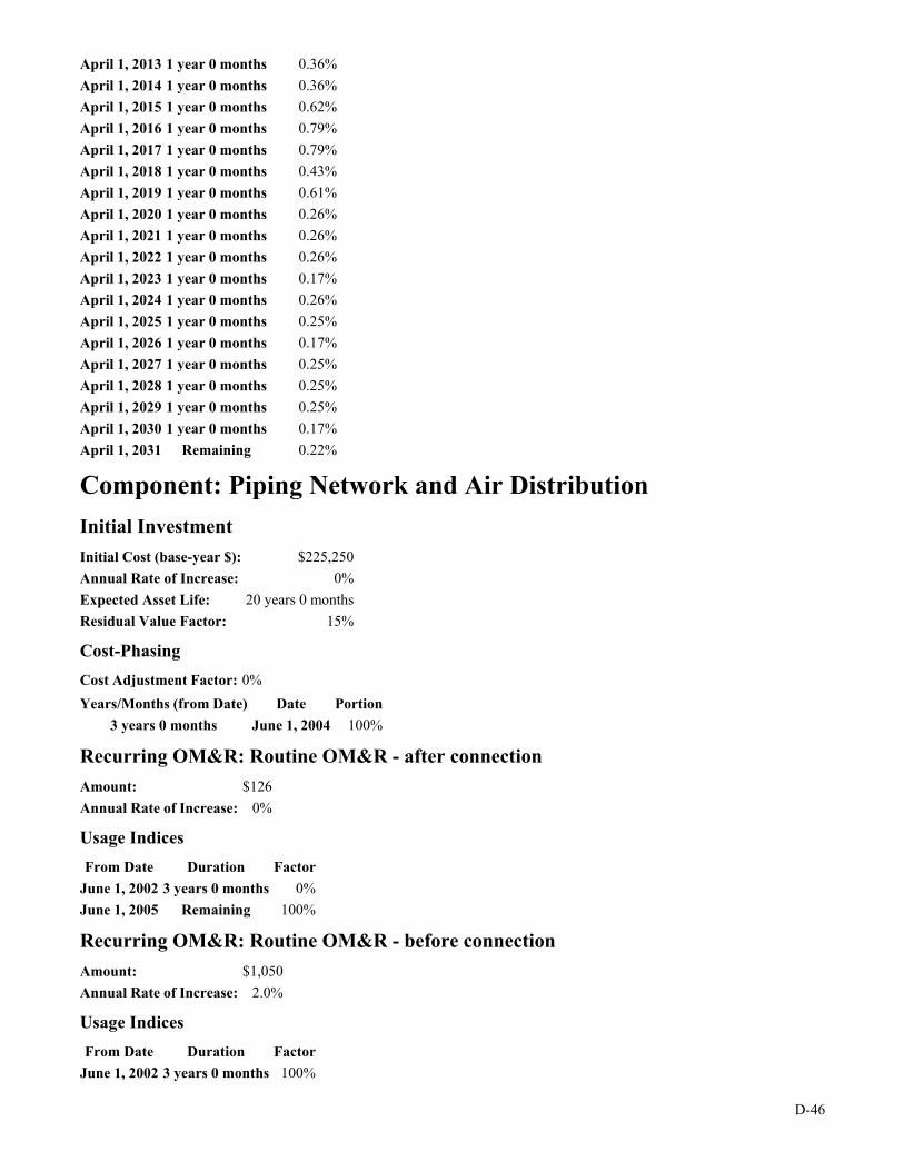
D-46

April 1, 2013 1 year 0 months 0.36% April 1, 2014 1 year 0 months 0.36% April 1, 2015 1 year 0 months 0.62% April 1, 2016 1 year 0 months 0.79% April 1, 2017 1 year 0 months 0.79% April 1, 2018 1 year 0 months 0.43% April 1, 2019 1 year 0 months 0.61% April 1, 2020 1 year 0 months 0.26% April 1, 2021 1 year 0 months 0.26% April 1, 2022 1 year 0 months 0.26% April 1, 2023 1 year 0 months 0.17% April 1, 2024 1 year 0 months 0.26% April 1, 2025 1 year 0 months 0.25% April 1, 2026 1 year 0 months 0.17% April 1, 2027 1 year 0 months 0.25% April 1, 2028 1 year 0 months 0.25% April 1, 2029 1 year 0 months 0.25% April 1, 2030 1 year 0 months 0.17% April 1, 2031 Remaining 0.22%

Component: Piping Network and Air Distribution Initial Investment Initial Cost (base-year $): $225,250 Annual Rate of Increase: 0% Expected Asset Life: 20 years 0 months Residual Value Factor: 15%

Cost-Phasing Cost Adjustment Factor: 0% Years/Months (from Date) Date Portion

3 years 0 months June 1, 2004 100%

Recurring OM&R: Routine OM&R - after connection Amount: $126 Annual Rate of Increase: 0%

Usage Indices From Date Duration Factor

June 1, 2002 3 years 0 months 0% June 1, 2005 Remaining 100%

Recurring OM&R: Routine OM&R - before connection Amount: $1,050 Annual Rate of Increase: 2.0%

Usage Indices From Date Duration Factor

June 1, 2002 3 years 0 months 100%

D-47

June 1, 2005 Remaining 0%

Non-Recurring OM&R: Scheduled Repair1 Years/Months: 6 years 0 months Amount: $950 Annual Rate of Increase: 0%

Non-Recurring OM&R: Scheduled Repair2 Years/Months: 12 years 0 months Amount: $950 Annual Rate of Increase: 0%

Non-Recurring OM&R: Scheduled Repair3 Years/Months: 18 years 0 months Amount: $950 Annual Rate of Increase: 0%

Alternative: DX Split System w/higher E-cost Comment: Install split-system central AC unit. Sensitivity Analysis with 35% increase in energy costs

Energy: Electricity Annual Consumption: 162,446.0 kWh Price per Unit: $0.08711 Demand Charge: $0 Utility Rebate: $0 Location: Virginia Rate Schedule: Industrial State: Virginia

Usage Indices From Date Duration Usage Index

June 1, 2002 Remaining 100%

Escalation Rates From Date Duration Escalation

April 1, 2001 1 year 0 months -1.99% April 1, 2002 1 year 0 months -1.22% April 1, 2003 1 year 0 months -0.25% April 1, 2004 1 year 0 months -1.32% April 1, 2005 1 year 0 months -1.09% April 1, 2006 1 year 0 months -1.52% April 1, 2007 1 year 0 months -1.2% April 1, 2008 1 year 0 months -0.87% April 1, 2009 1 year 0 months -0.35% April 1, 2010 1 year 0 months -0.79% April 1, 2011 1 year 0 months -0.8% April 1, 2012 1 year 0 months -0.27% April 1, 2013 1 year 0 months 0.36% April 1, 2014 1 year 0 months 0.36%

D-48

April 1, 2015 1 year 0 months 0.62% April 1, 2016 1 year 0 months 0.79% April 1, 2017 1 year 0 months 0.79% April 1, 2018 1 year 0 months 0.43% April 1, 2019 1 year 0 months 0.61% April 1, 2020 1 year 0 months 0.26% April 1, 2021 1 year 0 months 0.26% April 1, 2022 1 year 0 months 0.26% April 1, 2023 1 year 0 months 0.17% April 1, 2024 1 year 0 months 0.26% April 1, 2025 1 year 0 months 0.25% April 1, 2026 1 year 0 months 0.17% April 1, 2027 1 year 0 months 0.25% April 1, 2028 1 year 0 months 0.25% April 1, 2029 1 year 0 months 0.25% April 1, 2030 1 year 0 months 0.17% April 1, 2031 Remaining 0.22%

Component: Copy of: AC System and Air Distribution Initial Investment Initial Cost (base-year $): $210,000 Annual Rate of Increase: 0% Expected Asset Life: 20 years 0 months Residual Value Factor: 0%

Cost-Phasing Cost Adjustment Factor: 0% Years/Months (from Date) Date Portion

0 years 0 months June 1, 2001 100%

Replacement: Compressor/Condens Years/Months: 15 years 0 months Amount: $31,130 Annual Rate Of Increase: 0% Expected Asset Life: 15 years 0 months Residual Value Factor: 67%

Recurring OM&R: Routine OM&R Amount: $530Annual Rate of Increase: 0%

Usage Indices From Date Duration Factor

June 1, 2002 Remaining 100%

D-49

Non-Recurring OM&R: Scheduled Repair1 Years/Months: 5 years 0 months Amount: $6,300 Annual Rate of Increase: 0%

Non-Recurring OM&R: Scheduled Repair2 Years/Months: 10 years 0 months Amount: $6,300 Annual Rate of Increase: 0%

Non-Recurring OM&R: Scheduled Repair3 Years/Months: 15 years 0 months Amount: $6,300 Annual Rate of Increase: 0%

D-50

NIST BLCC 5.0-01: Lowest LCC Consistent with Federal Life Cycle Cost Methodology and Procedures, 10 CFR, Part 436, Subpart A

General Information File Name: C:\Program Files\BLCC5\projects\Class Exercise D2.xml Run Date: Thu Sep 20 11:18:23 EDT 2001 Analysis Type: Federal Analysis, Agency-Funded Project Project Name: Class Exercise D2 Project Location: Virginia Analyst: SKF

Comment: Provide economical and effective air conditioning for the family housing office at the Dahlgren, VA Naval Station.

Base Date: June 1, 2001 Service Date: June 1, 2002 Study Period: 21 years 0 months (June 1, 2001 through May 31, 2022) Discount Rate: 3.3% Discounting Convention: Mid-Year

Lowest LCC Comparative Present-Value Costs of Alternatives

(Shown in Ascending Order of Initial Cost, * = Lowest LCC)

Alternative Initial Cost (PV) Life Cycle Cost (PV)

Existing System $0 $372,359 Postponed Central Plant Connection $204,340 $363,854 * DX Split System $210,000 $377,070

DX Split System w/higher E-cost $210,000 $425,446

Central Plant Connection $265,000 $398,039

D-51

NIST BLCC 5.0-01: Summary LCC Consistent with Federal Life Cycle Cost Methodology and Procedures, 10 CFR, Part 436, Subpart A

General Information File Name: C:\Program Files\BLCC5\projects\Class Exercise D2.xml Run Date: Thu Sep 20 11:20:22 EDT 2001 Analysis Type: Federal Analysis, Agency-Funded Project Project Name: Class Exercise D2 Project Location: Virginia Analyst: SKF

Comment: Provide economical and effective air conditioning for the family housing office at the Dahlgren, VA Naval Station.

Base Date: June 1, 2001 Service Date: June 1, 2002 Study Period: 21 years 0 months (June 1, 2001 through May 31, 2022) Discount Rate: 3.3% Discounting Convention: Mid-Year

Discount and Escalation Rates are REAL (exclusive of general inflation)

Alternative: Existing System LCC Summary Present Value Annual Value Initial Cost $0 $0 Energy Consumption Costs $333,102 $22,241 Energy Demand Costs $0 $0 Energy Utility Rebates $0 $0 Water Usage Costs $0 $0 Water Disposal Costs $0 $0 Annually Recurring OM&R Costs $18,318 $1,223 Non-Annually Recurring OM&R Costs $20,939 $1,398 Replacement Costs $0 $0 Less Remaining Value $0 $0

------------ ------------Total Life-Cycle Cost $372,359 $24,862

Alternative: DX Split System LCC Summary Present Value Annual Value Initial Cost $210,000 $14,021 Energy Consumption Costs $138,214 $9,228 Energy Demand Costs $0 $0Energy Utility Rebates $0 $0 Water Usage Costs $0 $0 Water Disposal Costs $0 $0

D-52

Annually Recurring OM&R Costs $7,547 $504 Non-Annually Recurring OM&R Costs $13,340 $891 Replacement Costs $18,517 $1,236 Less Remaining Value -$10,549 -$704

------------ ------------Total Life-Cycle Cost $377,070 $25,176

Alternative: Central Plant Connection LCC Summary Present Value Annual Value Initial Cost $265,000 $17,694 Energy Consumption Costs $128,646 $8,590 Energy Demand Costs $0 $0 Energy Utility Rebates $0 $0 Water Usage Costs $0 $0 Water Disposal Costs $0 $0 Annually Recurring OM&R Costs $1,794 $120 Non-Annually Recurring OM&R Costs $2,599 $174 Replacement Costs $0 $0 Less Remaining Value $0 $0

------------ ------------Total Life-Cycle Cost $398,039 $26,577

Alternative: Postponed Central Plant Connection LCC Summary Present Value Annual Value Initial Cost $204,340 $13,644 Energy Consumption Costs $170,211 $11,365Energy Demand Costs $0 $0 Energy Utility Rebates $0 $0 Water Usage Costs $0 $0 Water Disposal Costs $0 $0 Annually Recurring OM&R Costs $4,498 $300 Non-Annually Recurring OM&R Costs $1,892 $126 Replacement Costs $0 $0 Less Remaining Value -$17,088 -$1,141

------------ ------------Total Life-Cycle Cost $363,854 $24,294

D-53

Alternative: DX Split System w/higher E-cost LCC Summary Present Value Annual Value Initial Cost $210,000 $14,021 Energy Consumption Costs $186,590 $12,458 Energy Demand Costs $0 $0 Energy Utility Rebates $0 $0 Water Usage Costs $0 $0 Water Disposal Costs $0 $0 Annually Recurring OM&R Costs $7,547 $504 Non-Annually Recurring OM&R Costs $13,340 $891 Replacement Costs $18,517 $1,236 Less Remaining Value -$10,549 -$704

------------ ------------Total Life-Cycle Cost $425,446 $28,406

D-54

NIST BLCC 5.0-01: Comparative Analysis Consistent with Federal Life Cycle Cost Methodology and Procedures, 10 CFR, Part 436, Subpart A

Base Case: Existing System Alternative: DX Split System

General Information File Name: C:\Program Files\BLCC5\projects\Class Exercise D2.xml

Run Date: Thu Sep 20 11:21:33 EDT 2001

Project Name: Class Exercise D2

Project Location: Virginia

Analysis Type: Federal Analysis, Agency-Funded Project

Analyst: SKF

Comment Provide economical and effective air conditioning for the family housing office at the Dahlgren, VA Naval Station.

Base Date of Study: June 1, 2001

Service Date: June 1, 2002

Study Period: 21 years 0 months(June 1, 2001 through May 31, 2022)

Discount Rate: 3.3%

Discounting Convention: Mid-Year

Comparison of Present-Value Costs PV Life-Cycle Cost Base Case Alternative Savings from Alternative

Initial Investment Costs: Capital Requirements as of Base Date $0 $210,000 -$210,000

Future Costs: Energy Consumption Costs $333,102 $138,214 $194,887 Energy Demand Charges $0 $0 $0 Energy Utility Rebates $0 $0 $0 Water Costs $0 $0 $0 Recurring and Non-Recurring OM&R Costs $39,257 $20,888 $18,369 Capital Replacements $0 $18,517 -$18,517 Residual Value at End of Study Period $0 -$10,549 $10,549

------------ ------------ ------------

Subtotal (for Future Cost Items) $372,359 $167,070 $205,288

D-55

------------ ------------ ------------

Total PV Life-Cycle Cost $372,359 $377,070 -$4,712

Net Savings from Alternative Compared with Base Case PV of Non-Investment Savings $213,257 - Increased Total Investment $217,969

------------

Net Savings -$4,712

Savings-to-Investment Ratio (SIR) SIR = 0.98

SIR is lower than 1.0; project alternative is not cost effective.

Adjusted Internal Rate of Return AIRR = 3.19%

AIRR is lower than your discount rate; project alternative is not cost effective.

Payback Period Estimated Years to Payback (from beginning of Service Period) Simple Payback occurs in year 15 Simple Payback is negated in year 16 Simple Payback occurs in year 17

Energy Savings Summary Energy Savings Summary (in stated units) Energy -----Average Annual Consumption----- Life-Cycle Type Base Case Alternative Savings Savings Electricity 290,000.0 kWh 120,330.0 kWh 169,670.0 kWh 3,392,935.5 kWh

Energy Savings Summary (in MBtu) Energy -----Average Annual Consumption----- Life-Cycle Type Base Case Alternative Savings Savings Electricity 989.5 MBtu 410.6 MBtu 578.9 MBtu 11,577.2 MBtu

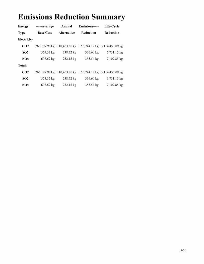
D-56

Emissions Reduction Summary Energy -----Average Annual Emissions----- Life-Cycle Type Base Case Alternative Reduction Reduction

Electricity CO2 266,197.98 kg 110,453.80 kg 155,744.17 kg 3,114,457.09 kg

SO2 575.32 kg 238.72 kg 336.60 kg 6,731.15 kg

NOx 607.69 kg 252.15 kg 355.54 kg 7,109.85 kg

Total: CO2 266,197.98 kg 110,453.80 kg 155,744.17 kg 3,114,457.09 kg

SO2 575.32 kg 238.72 kg 336.60 kg 6,731.15 kg

NOx 607.69 kg 252.15 kg 355.54 kg 7,109.85 kg

E-1

Module EReplace Chiller or Purchase Chilled Water

• compare LCCs of capital investments andoutsourcing,

• and when to include inflation estimates in federalLCCAs,

• use BLCC to evaluate contracted costs thatinclude inflation adjustments.

Objectives: Upon completion of this module, you will know how to

E-2

Pros and Cons of Chiller Replacementversus Chilled Water Contract

• CHILLER REPLACEMENT:High initial investment costSignificant maintenance (building engineer needed on site)Fixed output capacityScheduled shutdowns may be inconvenient or impracticalPerformance degradation over timeNot subject to contract renewal negotiations -- less uncertainty

• CHILLED WATER CONTRACT:Flexible contract lengthLow initial costNegligible maintenanceFlexible capacityHigher reliability; no down time for maintenanceMetered outputContract subject to renegotiation at expiration (uncertainty)

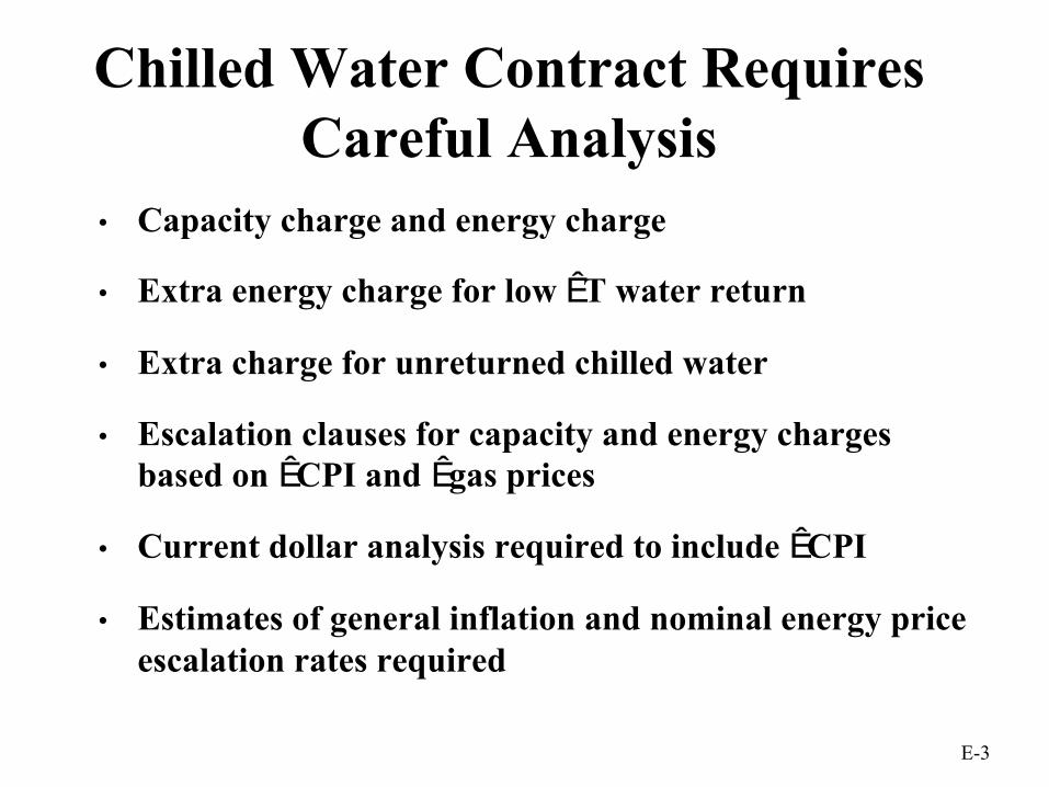
E-3

Chilled Water Contract RequiresCareful Analysis

• Capacity charge and energy charge

• Extra energy charge for low ªT water return

• Extra charge for unreturned chilled water

• Escalation clauses for capacity and energy chargesbased on ªCPI and ªgas prices

• Current dollar analysis required to include ªCPI

• Estimates of general inflation and nominal energy priceescalation rates required

E-4

Exercise E1230 Ton Chiller Replacement in Federal Building in Texas vs. Chilled Water Contract

Chiller Replacement:

Initial cost = $350,000Annual kWh cost (450,000 kWh @ $0.05/kWh) = $22,500Annual kW demand charge = $5,000Annual make-up water cost = $2,100Annual in-house labor = $10,000Annual service contract/supplies = $5,000Expected life = 20 years with refurbishment at end of year 10

(@ 40% of initial cost)Residual value = 0

E-5

Chilled Water Contract Proposal• Contract life negotiable:

– Capacity (demand) charges:– Monthly capacity charge = $13.00/ton– Excess capacity charge = $13.00/ton– Excess capacity “ratchet” = 12 months– Partially subject to annual CPI adjustment:– Adj. factor = 0.40 (Pt/Po) + 0.60 (CPIt / CPI0) where CPIt =

CPI in year t (CPI0 = CPI at start of contract)• Energy charges:

– Basic energy charge = $0.06/ton-h– Energy efficiency charge = $0.01/ton-h (based on ªT = 12F)– Energy charge subject to annual CPI and gas price

adjustmentsAdj. factor = 0.35 (Pt/P0) + 0.65 (CPIt / CPI0) where Pt = gasprice in year t (P0 = gas price at start of contract)

E-6

Current-Dollar or Constant-Dollar Analysis?

• Use constant dollars when contract includes generalinflation adjustment for all costs.

• Use current dollars when contract has differentescalation rates for different costs.

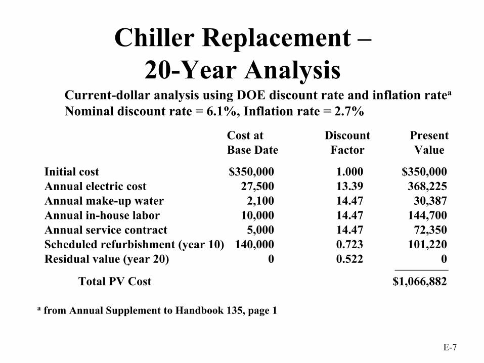
E-7

Chiller Replacement –20-Year Analysis

Current-dollar analysis using DOE discount rate and inflation ratea

Nominal discount rate = 6.1%, Inflation rate = 2.7%

Cost atBase Date

DiscountFactor

PresentValue

$350,00027,5002,100

10,0005,000

140,0000

1.00013.3914.4714.4714.470.7230.522

$350,000368,22530,387

144,70072,350

101,2200

Initial costAnnual electric costAnnual make-up waterAnnual in-house laborAnnual service contractScheduled refurbishment (year 10)Residual value (year 20)

$1,066,882Total PV Cost

a from Annual Supplement to Handbook 135, page 1

E-8

Purchase Chilled Water –20-Year Analysis

Cost (base date prices)

DiscountFactor

PresentValue

$10,000

14,352

21,528

9,55517,745

1.000

11.38

14.47a

12.01b

14.47

$10,000

163,326

311,510

114,756256,770

Initial system modificationAnnual costs (20 years):Basic capacity charge (230 tons)$35,880 Amount not subject to CPI adj. (40%)

Amount subject to CPI adj. (60%)Energy charge:(390,000 ton-hs@$0.07) $27,300 Amount subject to gas price adj. (35%) Amount subject to CPI adj. (65%)

$856,362Total 20-year cost

a Assumes 2.7% annual CPI increase, based on inflation assumption in ASHB135.b Based on DOE industrial gas price escalation rates for region 3 with 2.7% inflation.

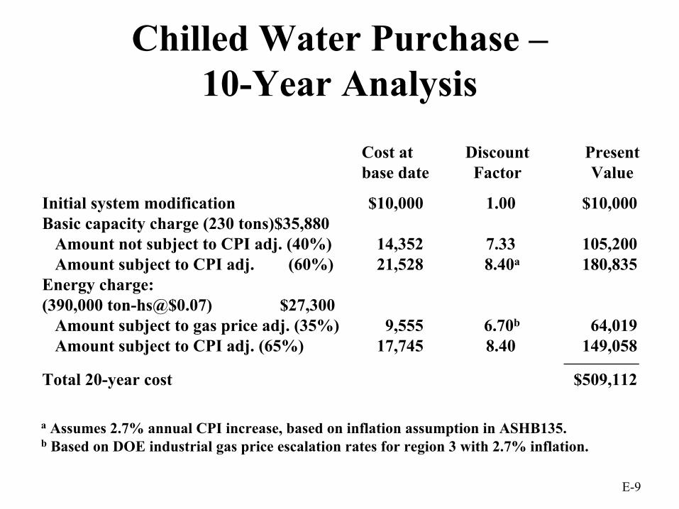
E-9

Chilled Water Purchase –10-Year Analysis

Cost at base date

DiscountFactor

PresentValue

$10,000

14,35221,528

9,55517,745

1.00

7.33 8.40a

6.70b

8.40

$10,000

105,200180,835

64,019149,058

Initial system modificationBasic capacity charge (230 tons)$35,880 Amount not subject to CPI adj. (40%) Amount subject to CPI adj. (60%)Energy charge:(390,000 ton-hs@$0.07) $27,300 Amount subject to gas price adj. (35%) Amount subject to CPI adj. (65%)

$509,112Total 20-year cost

a Assumes 2.7% annual CPI increase, based on inflation assumption in ASHB135.b Based on DOE industrial gas price escalation rates for region 3 with 2.7% inflation.

E-10

Cost atBase Date

DiscountFactor

PresentValue

$350,00027,5002,100

10,0005,000

35,000

1.007.898.408.408.40

0.723

$350,000216,97517,64084,00042,000

(25,305)

Initial costAnnual electric cCostAnnual make-up waterAnnual in-house laborAnnual service contractResidual value (year 10) *

$685,310Total PV Cost

Chiller Replacement –10-Year Analysis

*Residual value based on 10 years remaining of 20-year life,less needed refurbishment. $175,000 - $140,000 = $35,000

E-11

Chiller Replacement –Years 11 to 20

2.7% Inflation, 6.1% Discount RateCost atbase date

DiscountFactor

PresentValue

$350,00027,5002,100

10,0005,000

140,000175,000

0.723a

5.50b

6.07b

6.07b

6.07b

0.522c

0.522c

$253,050151,25012,74760,70030,35073,080

(91,350)

Initial costAnnual electric costAnnual make-up waterAnnual in-house laborAnnual Service contractScheduled refurbishment (year 10)Residual value (year 20)

$489,827Total PV Cost

a SPV* for year 10 (2.7% inflation)b UPV* for 20 years - UPV* for 10 years c SPV* for year 20 (2.7% inflation)

E-12

LCC Summary

10-Year AnalysisPV 10-year chiller replacement costPV 10-year chilled water contract cost

20-Year AnalysisPV 20-year chiller replacement costPV 20-year chilled water contract costPV 10-year contract with chiller replacement at year 11PV 10-year chilled water contract costPV 10-year chiller replacement at year 11

$685,310509,112

$1,066,882856,362

$509,112 + 489,827

$998,939

E-13

Set Project Information

E-14

Enter Electricity Use

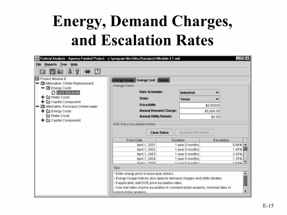
E-15

Energy, Demand Charges,and Escalation Rates

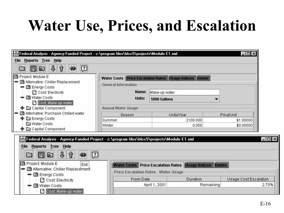
E-16

Water Use, Prices, and Escalation

E-17

Investment Costs

E-18

Annually Recurring OM&R Costs

E-19

Non-Annually RecurringOM&R Costs

E-20

Summary LCC forReplace Chiller Alternative

E-21

Purchase Chilled WaterAlternative

Energy costshave differingescalation rates

E-22

Non-Adjusted Capacity Cost

E-23

CPI-Adjusted Capacity Cost

E-24

DOE-Escalated Natural Gas

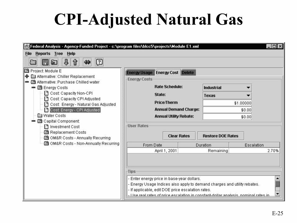
E-25

CPI-Adjusted Natural Gas

E-26

Investment Cost

E-27

Summary LCC forPurchase Chilled Water Alternative

E-28

Class Exercise E2PROBLEM STATEMENT

The building energy coordinator has reviewed the analysis and has concluded that given presentnatural gas prices and DOE projections for energy escalation, it is cost-effective to enter into acontract to purchase chilled-water.

However, he is concerned about the changing price and availability of natural gas resulting fromdecreasing supplies and a national trend towards summer peak electrical generation using naturalgas. As a result, he wants to determine the rate of natural gas price escalation that will make hisdecision to purchase chilled water a bad decision, i.e. not cost-effective.

His contract with the chilled water supplier is for a minimum of five years. Determine thebreakeven natural gas price for a five-year study period. The breakeven gas price will be the onewhere the net savings is zero (equal life-cycle costs for both alternatives).

Note: The chiller’s residual value will change based on the study period. Also, the chillerrefurbishment is not planned until the tenth year. For the analysis, assume the residual value of thechiller for the five-year study period is 75 %.

E-29

Class Exercise E3PROBLEM STATEMENT

The manager of the buildings is still uncertain about leaving the supply of chilled water up to a third party. He hasasked you to compare the life-cycle cost of purchasing chilled water for a 20-year period versus purchasing chilledwater for 10 years and then buying a chiller.

To purchase chilled water for 10 years and then purchase a chiller has the following costs:

Purchase chilled water contract cost = $10,000

Purchase chiller in year 10 = $350,000

First 10 years

Capacity charge, $35,880, of which 40 % is not adjusted and 60 % is adjusted for inflation.

Energy charge, $27,300, of which 35 % is adjusted for changing natural gas prices and 65 % is adjusted for inflation.

Years 11-20

Energy costs for 450,000 kWh at $0.05 per kWh plus $5,000 demand charges, both adjusted for changingelectricity prices.

Make-up water costs of $2,100 annually, adjusted for inflation.

In-house labor of $2,100 annually.

Service contract of $5,000 annually.

The chiller residual value after 10 years of use and needing a refurbishment will be $350,000/2 –$140,000 = $35,000 orten percent.

E-30

Solution to Class Exercise E2 NIST BLCC 5.0-01: Input Data Listing Consistent with Federal Life Cycle Cost Methodology and Procedures, 10 CFR, Part 436, Subpart A

General Information File Name: C:\Program Files\BLCC5\projects\Class Exercise

E2.xml Run Date: Thu Sep 20 11:34:24 EDT 2001 Analysis Type: Federal Analysis, Agency-Funded Project Project Name: Class Exercise E2 Project Location: Texas Analyst: GMM Comment: Replace Chiller or Purchase Chilled Water. Base Date: April 1, 2001 Service Date: April 1, 2001

Study Period: 5 years 0 months (April 1, 2001 through March 31, 2006)

Discount Rate: 6.1% Discounting Convention: End-of-Year

Discount and Escalation Rates are NOMINAL (inclusive of general inflation)

Alternative: Chiller Replacement Energy: Electricity Annual Consumption: 450,000.0 kWh Price per Unit: $0.05000 Demand Charge: $5,000 Utility Rebate: $0 Location: U.S. Average Rate Schedule: Industrial State: Texas

Usage Indices From Date Duration Usage Index

April 1, 2001 Remaining 100%

Escalation Rates From Date Duration Escalation

April 1, 2001 1 year 0 months 0.66% April 1, 2002 1 year 0 months 1.45% April 1, 2003 1 year 0 months 2.45% April 1, 2004 1 year 0 months 1.35% April 1, 2005 1 year 0 months 1.59% April 1, 2006 1 year 0 months 1.14% April 1, 2007 1 year 0 months 1.47% April 1, 2008 1 year 0 months 1.81%

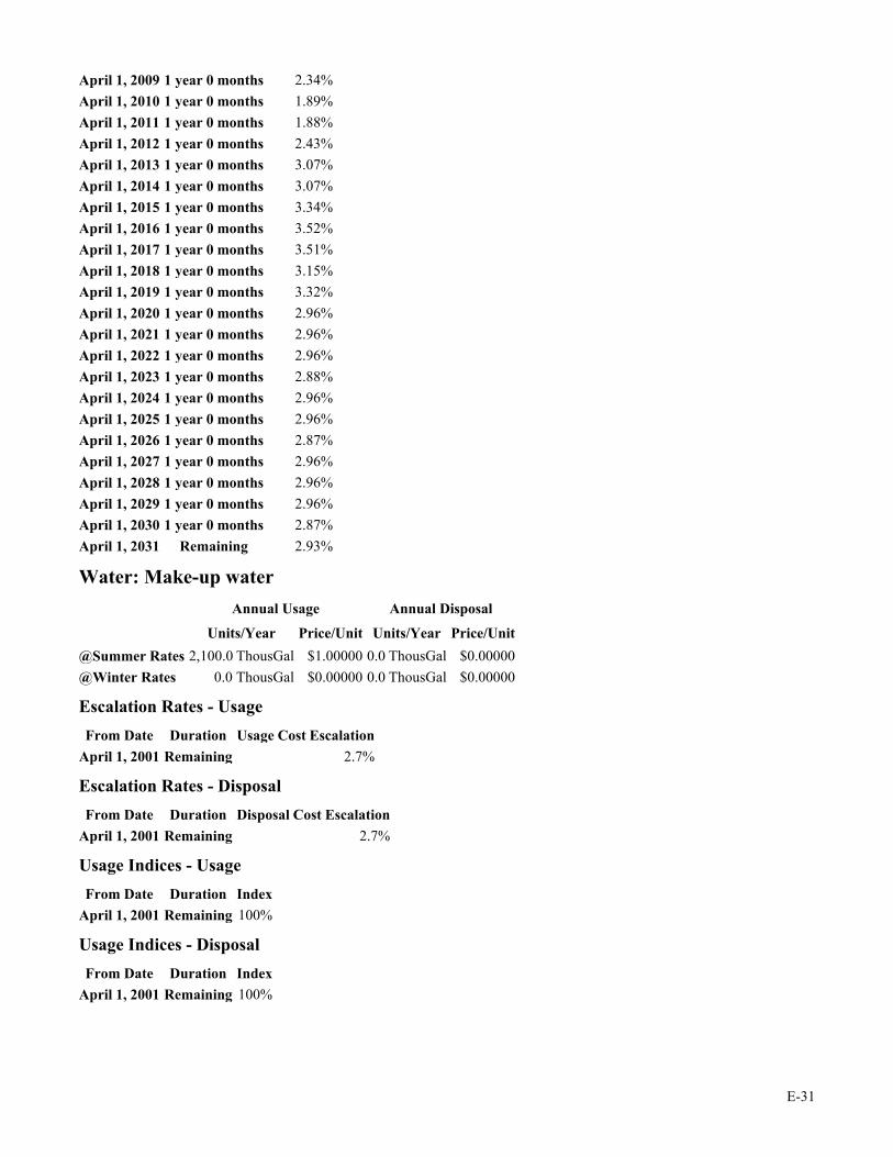
E-31

April 1, 2009 1 year 0 months 2.34% April 1, 2010 1 year 0 months 1.89% April 1, 2011 1 year 0 months 1.88% April 1, 2012 1 year 0 months 2.43% April 1, 2013 1 year 0 months 3.07% April 1, 2014 1 year 0 months 3.07% April 1, 2015 1 year 0 months 3.34% April 1, 2016 1 year 0 months 3.52% April 1, 2017 1 year 0 months 3.51% April 1, 2018 1 year 0 months 3.15% April 1, 2019 1 year 0 months 3.32% April 1, 2020 1 year 0 months 2.96% April 1, 2021 1 year 0 months 2.96% April 1, 2022 1 year 0 months 2.96% April 1, 2023 1 year 0 months 2.88% April 1, 2024 1 year 0 months 2.96% April 1, 2025 1 year 0 months 2.96% April 1, 2026 1 year 0 months 2.87% April 1, 2027 1 year 0 months 2.96% April 1, 2028 1 year 0 months 2.96% April 1, 2029 1 year 0 months 2.96% April 1, 2030 1 year 0 months 2.87% April 1, 2031 Remaining 2.93%

Water: Make-up water Annual Usage Annual Disposal Units/Year Price/Unit Units/Year Price/Unit @Summer Rates 2,100.0 ThousGal $1.00000 0.0 ThousGal $0.00000 @Winter Rates 0.0 ThousGal $0.00000 0.0 ThousGal $0.00000

Escalation Rates - Usage From Date Duration Usage Cost Escalation

April 1, 2001 Remaining 2.7%

Escalation Rates - Disposal From Date Duration Disposal Cost Escalation

April 1, 2001 Remaining 2.7%

Usage Indices - Usage From Date Duration Index

April 1, 2001 Remaining 100%

Usage Indices - Disposal From Date Duration Index

April 1, 2001 Remaining 100%

E-32

Component: Initial Investment Initial Cost (base-year $): $350,000 Annual Rate of Increase: 2.7% Expected Asset Life: 20 years 0 months Residual Value Factor: 75%

Cost-Phasing Cost Adjustment Factor: 2.7% Years/Months (from Date) Date Portion

0 years 0 months April 1, 2001 100%

Recurring OM&R: Labor Amount: $10,000 Annual Rate of Increase: 2.7%

Usage Indices From Date Duration Factor

April 1, 2001 Remaining 100%

Recurring OM&R: Service Contract Amount: $5,000 Annual Rate of Increase: 2.7%

Usage Indices From Date Duration Factor

April 1, 2001 Remaining 100%

Alternative: Purchase Chilled water Energy: Capacity Non-CPI Annual Consumption: 0.0 kWh Price per Unit: $0.00000 Demand Charge: $14,352 Utility Rebate: $0 Location: U.S. Average Rate Schedule: Industrial State: Texas

Usage Indices From Date Duration Usage Index

April 1, 2001 Remaining 100%

Escalation Rates From Date Duration Escalation

April 1, 2001 Remaining 0%

E-33

Energy: Capacity CPI Adjusted Annual Consumption: 0.0 kWh Price per Unit: $0.00000 Demand Charge: $21,528 Utility Rebate: $0 Location: U.S. Average Rate Schedule: Industrial State: Texas

Usage Indices From Date Duration Usage Index

April 1, 2001 Remaining 100%

Escalation Rates From Date Duration Escalation

Energy: Energy - Natural Gas Adjusted Annual Consumption: 9,555.0 Therm Price per Unit: $1.00000 Demand Charge: $0 Utility Rebate: $0 End-Use: Industrial Boiler, uncontrolled Rate Schedule: Industrial State: Texas

Usage Indices From Date Duration Usage Index

April 1, 2001 Remaining 100%

Escalation Rates From Date Duration Escalation

April 1, 2001 Remaining 23%

Energy: Energy - CPI Adjusted Annual Consumption: 17,745.0 Therm Price per Unit: $1.00000 Demand Charge: $0 Utility Rebate: $0 End-Use: Industrial Boiler, uncontrolled Rate Schedule: Industrial State: Texas

Usage Indices From Date Duration Usage Index

April 1, 2001 Remaining 100%

Escalation Rates From Date Duration Escalation

April 1, 2001 Remaining 2.7%

E-34

Component: Initial Investment Initial Cost (base-year $): $10,000 Annual Rate of Increase: 2.7% Expected Asset Life: 20 years 0 months Residual Value Factor: 0%

Cost-Phasing Cost Adjustment Factor: 2.7% Years/Months (from Date) Date Portion

0 years 0 months April 1, 2001 100%

E-35

Breakeven Analysis for Purchase Chiller versus Chilled Water

Nominal Escalation Rate Net Savings LCC Chiller LCC Chilled Water2.7% $32,757 $324,737 $291,9807.7% $26,159 $324,737 $298,578

12.7% $18,684 $324,737 $306,05317.7% $10,237 $324,737 $314,50022.7% $717 $324,737 $324,02027.7% -$9,987 $324,737 $334,724

Breakeven occurs at about 23 percent nominal escalation rate.

Net Savings versus Natural Gas Escalation

-$15,000-$10,000-$5,000

$0$5,000

$10,000$15,000$20,000$25,000$30,000$35,000

0.0% 5.0% 10.0% 15.0% 20.0% 25.0% 30.0%

Natural Gas Nominal Escalation Rate

Net

Sav

ings

E-36

Solution to Class Exercise E3 NIST BLCC 5.0-01: Input Data Listing Consistent with Federal Life Cycle Cost Methodology and Procedures, 10 CFR, Part 436, Subpart A

General Information File Name: C:\Program Files\BLCC5\projects\Class Exercise E3.xml Run Date: Thu Sep 20 11:51:03 EDT 2001 Analysis Type: Federal Analysis, Agency-Funded Project Project Name: Class Exercise E3 Project Location: Texas Analyst: GMM

Comment: Purchase chilled water for 10 years and then chiller versus purchase chilled water for 20 years

Base Date: April 1, 2001 Service Date: April 1, 2001 Study Period: 20 years 0 months (April 1, 2001 through March 31, 2021) Discount Rate: 6.1% Discounting Convention: End-of-Year

Discount and Escalation Rates are NOMINAL (inclusive of general inflation)

Alternative: Chilled water and then chiller Energy: Capacity - Non CPI Annual Consumption: 0.0 kWh Price per Unit: $0.00000 Demand Charge: $14,352 Utility Rebate: $0 End-Use: Industrial Boiler, uncontrolled Rate Schedule: Industrial State: Texas

Usage Indices From Date Duration Usage Index

April 1, 2001 10 years 0 months 100% April 1, 2011 Remaining 0%

Escalation Rates From Date Duration Escalation

April 1, 2001 Remaining 0%

Energy: Natural Gas Annual Consumption: 9,555.0 Therm Price per Unit: $1.00000 Demand Charge: $0 Utility Rebate: $0 End-Use: Industrial Boiler, uncontrolled

E-37

Rate Schedule: Industrial State: Texas

Usage Indices From Date Duration Usage Index

April 1, 2001 10 years 0 months 100% April 1, 2011 Remaining 0%

Escalation Rates From Date Duration Escalation

April 1, 2001 1 year 0 months -8.86% April 1, 2002 1 year 0 months -7.90% April 1, 2003 1 year 0 months -2.37% April 1, 2004 1 year 0 months 3.06% April 1, 2005 1 year 0 months 4.12% April 1, 2006 1 year 0 months 4.45% April 1, 2007 1 year 0 months 4.42% April 1, 2008 1 year 0 months 3.38% April 1, 2009 1 year 0 months 3.71% April 1, 2010 1 year 0 months 3.36% April 1, 2011 1 year 0 months 3.36% April 1, 2012 1 year 0 months 4.01% April 1, 2013 1 year 0 months 3.67% April 1, 2014 1 year 0 months 4.30% April 1, 2015 1 year 0 months 4.28% April 1, 2016 1 year 0 months 4.57% April 1, 2017 1 year 0 months 4.53% April 1, 2018 1 year 0 months 4.80% April 1, 2019 1 year 0 months 5.35% April 1, 2020 1 year 0 months 4.42% April 1, 2021 1 year 0 months 4.11% April 1, 2022 1 year 0 months 3.81% April 1, 2023 1 year 0 months 4.08% April 1, 2024 1 year 0 months 4.06% April 1, 2025 1 year 0 months 4.04% April 1, 2026 1 year 0 months 4.02% April 1, 2027 1 year 0 months 4.01% April 1, 2028 1 year 0 months 3.99% April 1, 2029 1 year 0 months 4.23% April 1, 2030 1 year 0 months 3.96% April 1, 2031 Remaining 4.04%

Energy: Capacity - CPI adjusted Annual Consumption: 0.0 kWh Price per Unit: $0.00000 Demand Charge: $21,528 Utility Rebate: $0 End-Use: Industrial Boiler, uncontrolled

E-38

Rate Schedule: Industrial State: Texas

Usage Indices From Date Duration Usage Index

April 1, 2001 10 years 0 months 100% April 1, 2011 Remaining 0%

Escalation Rates From Date Duration Escalation

April 1, 2001 Remaining 2.7%

Energy: Energy - CPI adjusted Annual Consumption: 17,745.0 Therm Price per Unit: $1.00000 Demand Charge: $0 Utility Rebate: $0 End-Use: Industrial Boiler, uncontrolled Rate Schedule: Industrial State: Texas

Usage Indices From Date Duration Usage Index

April 1, 2001 10 years 0 months 100% April 1, 2011 Remaining 0%

Escalation Rates From Date Duration Escalation

April 1, 2001 Remaining 2.7%

Energy: Electricity Annual Consumption: 450,000.0 kWh Price per Unit: $0.05000 Demand Charge: $5,000 Utility Rebate: $0 Location: U.S. Average Rate Schedule: Industrial State: Texas

Usage Indices From Date Duration Usage Index

April 1, 2001 10 years 0 months 0% April 1, 2011 Remaining 100%

Escalation Rates From Date Duration Escalation

April 1, 2001 1 year 0 months 0.66% April 1, 2002 1 year 0 months 1.45% April 1, 2003 1 year 0 months 2.45%

E-39

April 1, 2004 1 year 0 months 1.35% April 1, 2005 1 year 0 months 1.59% April 1, 2006 1 year 0 months 1.14% April 1, 2007 1 year 0 months 1.47% April 1, 2008 1 year 0 months 1.81% April 1, 2009 1 year 0 months 2.34% April 1, 2010 1 year 0 months 1.89% April 1, 2011 1 year 0 months 1.88% April 1, 2012 1 year 0 months 2.43% April 1, 2013 1 year 0 months 3.07% April 1, 2014 1 year 0 months 3.07% April 1, 2015 1 year 0 months 3.34% April 1, 2016 1 year 0 months 3.52% April 1, 2017 1 year 0 months 3.51% April 1, 2018 1 year 0 months 3.15% April 1, 2019 1 year 0 months 3.32% April 1, 2020 1 year 0 months 2.96% April 1, 2021 1 year 0 months 2.96% April 1, 2022 1 year 0 months 2.96% April 1, 2023 1 year 0 months 2.88% April 1, 2024 1 year 0 months 2.96% April 1, 2025 1 year 0 months 2.96% April 1, 2026 1 year 0 months 2.87% April 1, 2027 1 year 0 months 2.96% April 1, 2028 1 year 0 months 2.96% April 1, 2029 1 year 0 months 2.96% April 1, 2030 1 year 0 months 2.87% April 1, 2031 Remaining 2.93%

Water: Make-up water Annual Usage Annual Disposal Units/Year Price/Unit Units/Year Price/Unit @Summer Rates 2,100.0 L $1.00000 0.0 L $0.00000 @Winter Rates 0.0 L $0.00000 0.0 L $0.00000

Escalation Rates - Usage From Date Duration Usage Cost Escalation

April 1, 2001 Remaining 2.7%

Escalation Rates - Disposal From Date Duration Disposal Cost Escalation

April 1, 2001 Remaining 2.7%

Usage Indices - Usage From Date Duration Index

April 1, 2001 10 years 0 months 0% April 1, 2011 Remaining 100%

E-40

Usage Indices - Disposal From Date Duration Index

April 1, 2001 Remaining 100%

Component: Purchase chilled water for 10 years Initial Investment Initial Cost (base-year $): $10,000 Annual Rate of Increase: 2.7% Expected Asset Life: 1 year 0 months Residual Value Factor: 0%

Cost-Phasing Cost Adjustment Factor: 2.7% Years/Months (from Date) Date Portion

0 years 0 months April 1, 2001 100%

Component: Purchase Chiller Initial Investment Initial Cost (base-year $): $350,000 Annual Rate of Increase: 2.7% Expected Asset Life: 20 years 0 months Residual Value Factor: 10%

Cost-Phasing Cost Adjustment Factor: 2.7% Years/Months (from Date) Date Portion

10 years 0 months April 1, 2011 100%

Recurring OM&R: In-house labor Amount: $10,000 Annual Rate of Increase: 2.7%

Usage Indices From Date Duration Factor

April 1, 2001 10 years 0 months 0% April 1, 2011 Remaining 100%

Recurring OM&R: Service contract Amount: $5,000 Annual Rate of Increase: 2.7%

Usage Indices From Date Duration Factor

April 1, 2001 10 years 0 months 0% April 1, 2011 Remaining 100%

E-41

Alternative: 20 Year Chilled Water Energy: Copy of: Capacity - Non CPI Annual Consumption: 0.0 kWh Price per Unit: $0.00000 Demand Charge: $14,352 Utility Rebate: $0 End-Use: Industrial Boiler, uncontrolled Rate Schedule: Industrial State: Texas

Usage Indices From Date Duration Usage Index

April 1, 2001 20 years 0 months 100% April 1, 2021 Remaining 100%

Escalation Rates From Date Duration Escalation

April 1, 2001 Remaining 0%

Energy: Copy of: Natural Gas Annual Consumption: 9,555.0 Therm Price per Unit: $1.00000 Demand Charge: $0 Utility Rebate: $0 End-Use: Industrial Boiler, uncontrolled Rate Schedule: Industrial State: Texas

Usage Indices From Date Duration Usage Index

April 1, 2001 20 years 0 months 100% April 1, 2021 Remaining 100%

Escalation Rates From Date Duration Escalation

April 1, 2001 1 year 0 months -8.86% April 1, 2002 1 year 0 months -7.90% April 1, 2003 1 year 0 months -2.37% April 1, 2004 1 year 0 months 3.06% April 1, 2005 1 year 0 months 4.12% April 1, 2006 1 year 0 months 4.45% April 1, 2007 1 year 0 months 4.42% April 1, 2008 1 year 0 months 3.38% April 1, 2009 1 year 0 months 3.71% April 1, 2010 1 year 0 months 3.36% April 1, 2011 1 year 0 months 3.36% April 1, 2012 1 year 0 months 4.01%

E-42

April 1, 2013 1 year 0 months 3.67% April 1, 2014 1 year 0 months 4.30% April 1, 2015 1 year 0 months 4.28% April 1, 2016 1 year 0 months 4.57% April 1, 2017 1 year 0 months 4.53% April 1, 2018 1 year 0 months 4.80% April 1, 2019 1 year 0 months 5.35% April 1, 2020 1 year 0 months 4.42% April 1, 2021 1 year 0 months 4.11% April 1, 2022 1 year 0 months 3.81% April 1, 2023 1 year 0 months 4.08% April 1, 2024 1 year 0 months 4.06% April 1, 2025 1 year 0 months 4.04% April 1, 2026 1 year 0 months 4.02% April 1, 2027 1 year 0 months 4.01% April 1, 2028 1 year 0 months 3.99% April 1, 2029 1 year 0 months 4.23% April 1, 2030 1 year 0 months 3.96% April 1, 2031 Remaining 4.04%

Energy: Copy of: Capacity - CPI adjusted Annual Consumption: 0.0 kWh Price per Unit: $0.00000 Demand Charge: $21,528 Utility Rebate: $0 End-Use: Industrial Boiler, uncontrolled Rate Schedule: Industrial State: Texas

Usage Indices From Date Duration Usage Index

April 1, 2001 20 years 0 months 100% April 1, 2021 Remaining 100%

Escalation Rates From Date Duration Escalation

April 1, 2001 Remaining 2.7%

Energy: Copy of: Energy - CPI adjusted Annual Consumption: 17,745.0 Therm Price per Unit: $1.00000 Demand Charge: $0 Utility Rebate: $0 End-Use: Industrial Boiler, uncontrolled Rate Schedule: Industrial State: Texas

Usage Indices From Date Duration Usage Index

E-43

April 1, 2001 20 years 0 months 100% April 1, 2021 Remaining 100%

Escalation Rates From Date Duration Escalation

April 1, 2001 Remaining 2.7%

Component: Copy of: Purchase chilled water for 10 years Initial Investment Initial Cost (base-year $): $10,000 Annual Rate of Increase: 2.7% Expected Asset Life: 1 year 0 months Residual Value Factor: 0%

Cost-Phasing Cost Adjustment Factor: 2.7% Years/Months (from Date) Date Portion

0 years 0 months April 1, 2001 100%

E-44

NIST BLCC 5.0-01: Detailed LCC Analysis Consistent with Federal Life Cycle Cost Methodology and Procedures, 10 CFR, Part 436, Subpart A

General Information File Name: C:\Program Files\BLCC5\projects\Class Exercise E3.xml Run Date: Thu Sep 20 13:25:39 EDT 2001 Analysis Type: Federal Analysis, Agency-Funded Project Project Name: Class Exercise E3 Project Location: Texas Analyst: GMM

Comment: Purchase chilled water for 10 years and then chiller versus purchase chilled water for 20 years

Base Date: April 1, 2001 Service Date: April 1, 2001 Study Period: 20 years 0 months (April 1, 2001 through March 31, 2021) Discount Rate: 6.1% Discounting Convention: End-of-Year

Discount and Escalation Rates are NOMINAL (inclusive of general inflation)

Alternative: Chilled water and then chiller Initial Cost Data (not Discounted) Initial Capital Costs (adjusted for price escalation)

Initial Capital Costs for All Components: $466,832

Component: Purchase chilled water for 10 years Cost-Phasing

Date Portion Yearly Cost April 1, 2001 100% $10,000

------------ ------------

Total (for Component) $10,000

Component: Purchase Chiller Cost-Phasing

Date Portion Yearly Cost April 1, 2011 100% $456,832

------------ ------------

Total (for Component) $456,832

Energy Costs: Capacity - Non CPI (base-year dollars)

Average Average Average Average Annual Usage Price/Unit Annual Cost Annual Demand Annual Rebate

0.0 kWh $0.00000 $0 $7,176 $0

E-45

Energy Costs: Natural Gas (base-year dollars)

Average Average Average Average Annual Usage Price/Unit Annual Cost Annual Demand Annual Rebate 4,777.5 Therm $1.00000 $4,778 $0 $0

Energy Costs: Capacity - CPI adjusted (base-year dollars)

Average Average Average Average Annual Usage Price/Unit Annual Cost Annual Demand Annual Rebate

0.0 kWh $0.00000 $0 $10,764 $0

Energy Costs: Energy - CPI adjusted (base-year dollars)

Average Average Average Average Annual Usage Price/Unit Annual Cost Annual Demand Annual Rebate 8,872.5 Therm $1.00000 $8,872 $0 $0

Energy Costs: Electricity (base-year dollars)

Average Average Average Average Annual Usage Price/Unit Annual Cost Annual Demand Annual Rebate 225,000.0 kWh $0.05000 $11,250 $2,500 $0

Water Costs: Make-up water (base-year dollars)

Average Annual Usage Average Annual Disposal Average Annual Water Units/Year Price/Unit Units/Year Price/Unit Cost @ Summer Rates 1,050.0 L $1.00000 0.0 L $0.00000 $1,050 @ Winter Rates 0.0 L $0.00000 0.0 L $0.00000 $0

Life-Cycle Cost Analysis Present Value Annual Value Initial Capital Costs $262,979 $23,095

Energy Costs Energy Consumption Costs $336,857 $29,584 Energy Demand Charges $313,579 $27,539 Energy Utility Rebates $0 $0

------------ ------------ Subtotal (for Energy): $650,437 $57,123

Water Usage Costs $12,753 $1,120 Water Disposal Costs $0 $0

Operating, Maintenance & Repair Costs

E-46

Component: Purchase chilled water for 10 years Annually Recurring Costs $0 $0 Non-Annually Recurring Costs $0 $0 Component: Purchase Chiller Annually Recurring Costs $91,089 $8,000 Non-Annually Recurring Costs $0 $0

------------ ------------ Subtotal (for OM&R): $91,089 $8,000

Replacements to Capital Components Component: Purchase chilled water for 10 years $0 $0 Component: Purchase Chiller $0 $0

------------ ------------ Subtotal (for Replacements): $0 $0

Residual Value of Original Capital Components Component: Purchase chilled water for 10 years $0 $0 Component: Purchase Chiller -$18,285 -$1,606

------------ ------------ Subtotal (for Residual Value): -$18,285 -$1,606

Residual Value of Capital Replacements Component: Purchase chilled water for 10 years $0 $0 Component: Purchase Chiller $0 $0

------------ ------------ Subtotal (for Residual Value): $0 $0

Total Life-Cycle Cost $998,972 $87,732

Emissions Summary Energy Name Annual Life-Cycle Capacity - Non CPI:

CO2 0.00 kg 0.00 kg SO2 0.00 kg 0.00 kg NOx 0.00 kg 0.00 kg

Natural Gas: CO2 25,236.45 kg 504,659.81 kg SO2 203.67 kg 4,072.76 kg NOx 29.74 kg 594.78 kg

Capacity - CPI adjusted: CO2 0.00 kg 0.00 kg SO2 0.00 kg 0.00 kg NOx 0.00 kg 0.00 kg

Energy - CPI adjusted: CO2 46,867.68 kg 937,225.37 kg

E-47

SO2 378.24 kg 7,563.70 kg NOx 55.24 kg 1,104.60 kg

Electricity: CO2 218,094.01 kg 4,361,283.00 kg SO2 664.29 kg 13,284.00 kg NOx 657.00 kg 13,138.20 kg

Total: CO2 290,198.14 kg 5,803,168.18 kg SO2 1,246.19 kg 24,920.47 kg NOx 741.98 kg 14,837.59 kg

Alternative: 20 Year Chilled Water Initial Cost Data (not Discounted) Initial Capital Costs (adjusted for price escalation)

Initial Capital Costs for All Components: $10,000

Component: Copy of: Purchase chilled water for 10 years Cost-Phasing

Date Portion Yearly Cost April 1, 2001 100% $10,000

------------ ------------

Total (for Component) $10,000

Energy Costs: Copy of: Capacity - Non CPI (base-year dollars)

Average Average Average Average Annual Usage Price/Unit Annual Cost Annual Demand Annual Rebate

0.0 kWh $0.00000 $0 $14,352 $0

Energy Costs: Copy of: Natural Gas (base-year dollars)

Average Average Average Average Annual Usage Price/Unit Annual Cost Annual Demand Annual Rebate 9,555.0 Therm $1.00000 $9,555 $0 $0

Energy Costs: Copy of: Capacity - CPI adjusted (base-year dollars)

Average Average Average Average Annual Usage Price/Unit Annual Cost Annual Demand Annual Rebate

0.0 kWh $0.00000 $0 $21,528 $0

Energy Costs: Copy of: Energy - CPI adjusted (base-year dollars)

Average Average Average Average Annual Usage Price/Unit Annual Cost Annual Demand Annual Rebate

E-48

17,745.0 Therm $1.00000 $17,745 $0 $0

Life-Cycle Cost Analysis Present Value Annual Value Initial Capital Costs $10,000 $878

Energy Costs Energy Consumption Costs $371,605 $32,635 Energy Demand Charges $475,072 $41,722 Energy Utility Rebates $0 $0

------------ ------------ Subtotal (for Energy): $846,676 $74,357

Water Usage Costs $0 $0 Water Disposal Costs $0 $0

Operating, Maintenance & Repair Costs Component: Copy of: Purchase chilled water for 10 years Annually Recurring Costs $0 $0 Non-Annually Recurring Costs $0 $0

------------ ------------ Subtotal (for OM&R): $0 $0

Replacements to Capital Components Component: Copy of: Purchase chilled water for 10 years $0 $0

------------ ------------ Subtotal (for Replacements): $0 $0

Residual Value of Original Capital Components Component: Copy of: Purchase chilled water for 10 years $0 $0

------------ ------------ Subtotal (for Residual Value): $0 $0

Residual Value of Capital Replacements Component: Copy of: Purchase chilled water for 10 years $0 $0

------------ ------------ Subtotal (for Residual Value): $0 $0

Total Life-Cycle Cost $856,676 $75,235

E-49

Emissions Summary Energy Name Annual Life-Cycle Copy of: Capacity - Non CPI:

CO2 0.00 kg 0.00 kg SO2 0.00 kg 0.00 kg NOx 0.00 kg 0.00 kg

Copy of: Natural Gas: CO2 50,472.89 kg 1,009,319.63 kg SO2 407.33 kg 8,145.53 kg NOx 59.49 kg 1,189.57 kg

Copy of: Capacity - CPI adjusted: CO2 0.00 kg 0.00 kg SO2 0.00 kg 0.00 kg NOx 0.00 kg 0.00 kg

Copy of: Energy - CPI adjusted: CO2 93,735.37 kg 1,874,450.74 kg SO2 756.47 kg 15,127.41 kg NOx 110.48 kg 2,209.20 kg

Total: CO2 144,208.26 kg 2,883,770.36 kg SO2 1,163.81 kg 23,272.94 kg NOx 169.96 kg 3,398.77 kg

E-50

NIST BLCC 5.0-01: Comparative Analysis Consistent with Federal Life Cycle Cost Methodology and Procedures, 10 CFR, Part 436, Subpart A

Base Case: Chilled water and then chiller Alternative: 20 Year Chilled Water

General Information File Name: C:\Program Files\BLCC5\projects\Class Exercise E3.xml Run Date: Thu Sep 20 11:54:01 EDT 2001 Project Name: Class Exercise E3 Project Location: Texas Analysis Type: Federal Analysis, Agency-Funded Project Analyst: GMM Comment Purchase chilled water for 10 years and then chiller versus purchase chilled water for 20 years Base Date of Study: April 1, 2001 Service Date: April 1, 2001 Study Period: 20 years 0 months(April 1, 2001 through March 31, 2021) Discount Rate: 6.1% Discounting Convention: End-of-Year

Comparison of Present-Value Costs PV Life-Cycle Cost Base Case Alternative Savings from Alternative

Initial Investment Costs: Capital Requirements as of Base Date $262,979 $10,000 $252,979 Future Costs: Energy Consumption Costs $336,857 $371,605 -$34,747 Energy Demand Charges $313,579 $475,072 -$161,492 Energy Utility Rebates $0 $0 $0 Water Costs $12,753 $0 $12,753 Recurring and Non-Recurring OM&R Costs $91,089 $0 $91,089 Capital Replacements $0 $0 $0 Residual Value at End of Study Period -$18,285 $0 -$18,285

------------ ------------ ------------ Subtotal (for Future Cost Items) $735,993 $846,676 -$110,683

------------ ------------ ------------ Total PV Life-Cycle Cost $998,972 $856,676 $142,296

Net Savings from Alternative Compared with Base Case PV of Non-Investment Savings -$92,398 - Increased Total Investment -$234,694

------------

E-51

Net Savings $142,296

Savings-to-Investment Ratio (SIR) SIR = 0.39

SIR is lower than 1.0; project alternative is not cost effective.

Adjusted Internal Rate of Return AIRR = 1.26%

AIRR is lower than your discount rate; project alternative is not cost effective.

Payback Period Estimated Years to Payback (from beginning of Service Period) Simple Payback occurs in year 1 Discounted Payback occurs in year 1

Energy Savings Summary Energy Savings Summary (in stated units) Units for every energy type not the same, can't report energy savings

Energy Savings Summary (in MBtu) Energy -----Average Annual Consumption----- Life-Cycle Type Base Case Alternative Savings Savings Electricity 767.7 MBtu 0.0 MBtu 767.7 MBtu 15,352.5 MBtu Natural Gas 1,365.0 MBtu 2,730.0 MBtu -1,365.0 MBtu -27,296.4 MBtu

Emissions Reduction Summary Energy -----Average Annual Emissions----- Life-Cycle Type Base Case Alternative Reduction Reduction Electricity

CO2 218,094.01 kg 0.00 kg 218,094.01 kg 4,361,283.00 kg SO2 664.29 kg 0.00 kg 664.29 kg 13,284.00 kg NOx 657.00 kg 0.00 kg 657.00 kg 13,138.20 kg

Natural Gas CO2 72,104.13 kg 144,208.26 kg -72,104.13 kg -1,441,885.18 kg SO2 581.90 kg 1,163.81 kg -581.90 kg -11,636.47 kg NOx 84.98 kg 169.96 kg -84.98 kg -1,699.39 kg

Total: CO2 290,198.14 kg 144,208.26 kg 145,989.88 kg 2,919,397.82 kg SO2 1,246.19 kg 1,163.81 kg 82.39 kg 1,647.53 kg NOx 741.98 kg 169.96 kg 572.02 kg 11,438.81 kg

F-1

Module FEvaluation of Alternative Financing Contracts

Objectives: Upon completion of this module, you will know how to

• structure alternative financing (AF) projects for LCCA.– Energy Savings Performance Contracts

(ESPCs)– Utility Energy Services Contracts (UCs)

• use BLCC5 to perform the analysis.

F-2

Steps in LCCA of AF Contracts

• Select the systems and equipment to impact and at what level.

• Perform LCCAs for individual ECMs.• Determine which ECMs to bundle.• Evaluate project for cost-effectiveness

compared with status quo or other strategies.

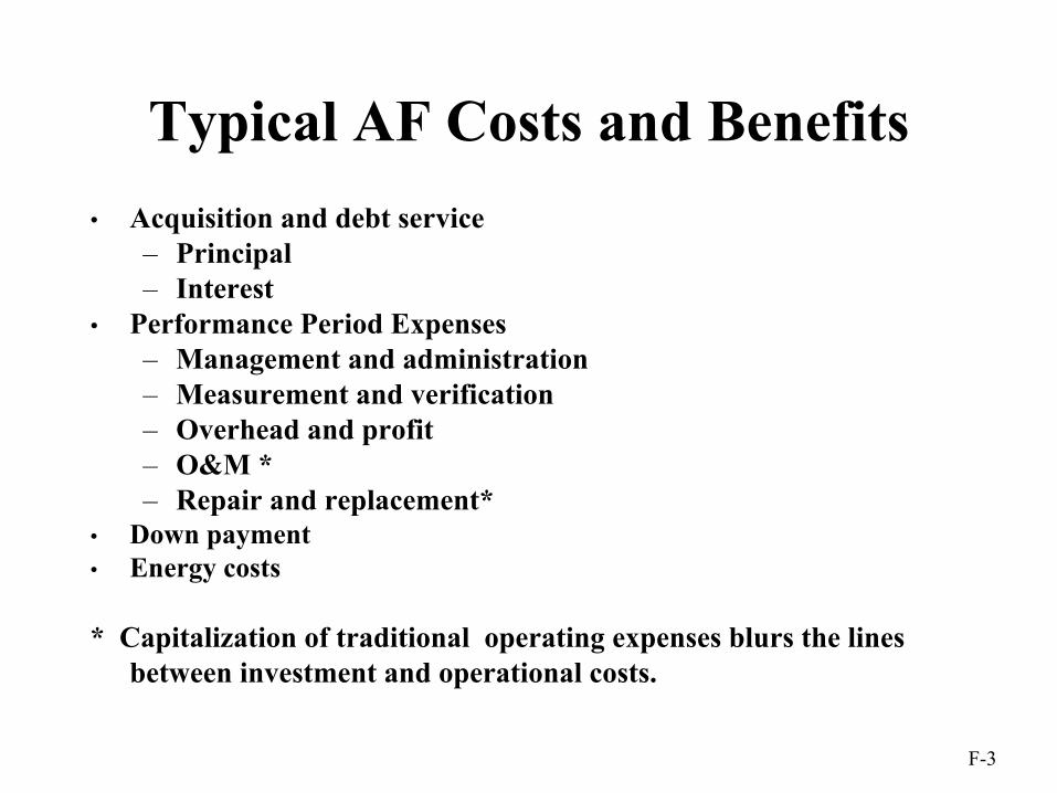
F-3

• Acquisition and debt service– Principal– Interest

• Performance Period Expenses– Management and administration– Measurement and verification– Overhead and profit– O&M *– Repair and replacement*

• Down payment• Energy costs

* Capitalization of traditional operating expenses blurs the linesbetween investment and operational costs.

Typical AF Costs and Benefits

F-4

Bundling of ECMs• Bundling of independent projects

– Each individual project should be cost-effective.– EO 13123 allows bundling of non-cost-effective

ECMs with those that generate high NS.– Bundling does not guarantee maximization of NS

for government investments overall.• Bundling of interdependent projects

– Analysts must account for interaction amongsystems.

– Energy consumption of different combinationsneeds to be recalculated.

F-5

Exercise F1Evaluation of ESPC Contract

PROBLEM STATEMENT

The building manager of the Jefferson Training Facility in Tennessee has been investigating thepossibility of financing, through an Energy Savings Performance Contract, an upgrade of the facility’shot water system and other energy conservation measures. In collaboration with an ESCO, she hasidentified five retrofit measures, which, according to the ESCO proposal, would result in operational costsavings of approximately $120K annually. With the current maintenance and repair schedule, theexisting system could be kept functional for another 25 years.

Options

Maintain status quo with current maintenance and repair schedule.

Install the following Energy Conservation Measures (ECMs:

1. Install new natural gas hot water boilers ($262,500).

2. Convert existing, electric DHW heating system to natural gas DHW system ($50,000).

3. Install campus-wide direct digital control (DDC) system ($412,500).

4. Improve lighting system ($250,000).

5. Convert constant HW and CW loops to variable flow ($187,500).

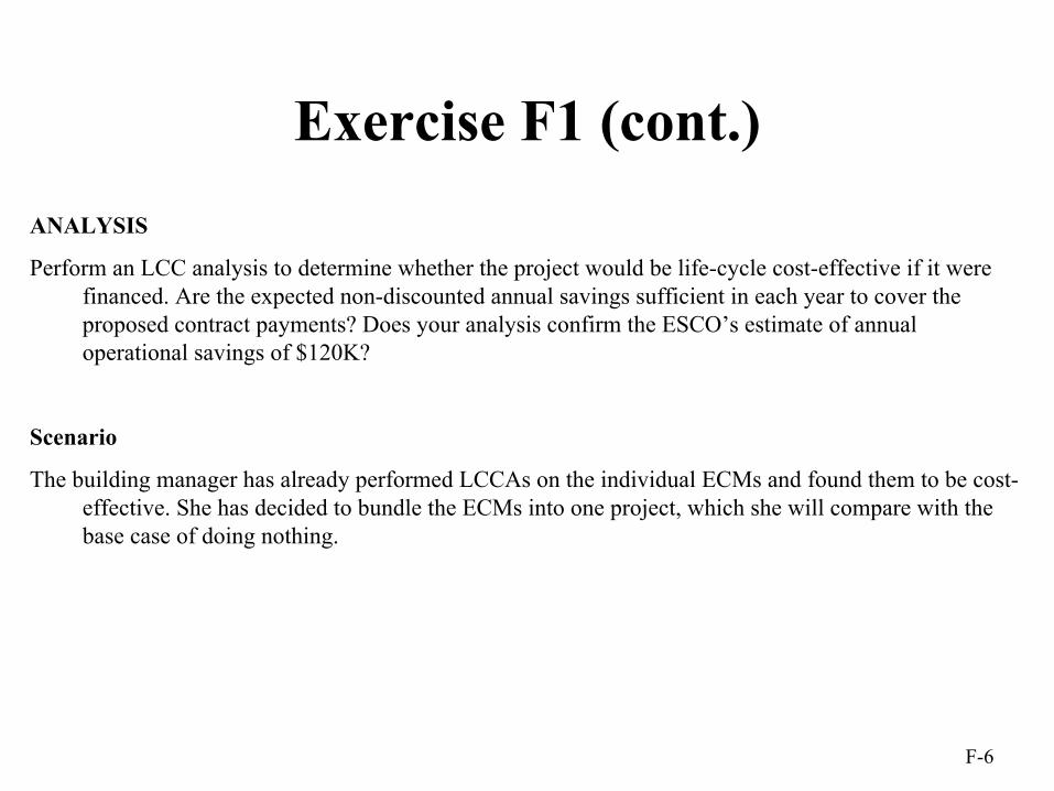
F-6

Exercise F1 (cont.)ANALYSIS

Perform an LCC analysis to determine whether the project would be life-cycle cost-effective if it were financed. Are the expected non-discounted annual savings sufficient in each year to cover the proposed contract payments? Does your analysis confirm the ESCO’s estimate of annual operational savings of $120K?

Scenario

The building manager has already performed LCCAs on the individual ECMs and found them to be cost-effective. She has decided to bundle the ECMs into one project, which she will compare with the base case of doing nothing.

F-7

General project information • ECMs in Training Facility, Jefferson, TN• current-dollar analysis• end-of-year discounting• discount rate: 6.1% nominal• inflation rate: 2.7%• DOE energy price escalation rates• all costs, except debt service payments, increase

at rate of inflation

F-8

Key Dates

• Base date: June 2001• Implementation period: 1 year• Service date: June 2002• Contract period: 20 years• Study period: 25 years

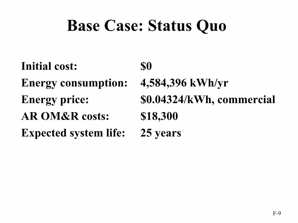
F-9

Base Case: Status Quo

Initial cost: $0Energy consumption: 4,584,396 kWh/yrEnergy price: $0.04324/kWh, commercialAR OM&R costs: $18,300Expected system life: 25 years

F-10

Alternative: ESPC Initial cost paid by agency: $29,283Total capital costs financed: $1,133,217Annual contract costs:

Debt service: $109,856, fixedPerformance period expenses: $7,047, increasing at 2.7%

Annual energy costs:pre-impl. period: Electricity: 4,584,396 kWh/yr

at $0.04324/kWh, commercialpost-impl. period: Natural Gas: 109,780 therms

at $0.46/therm, comm.

F-11

Alternative: ESPC (cont.)

AR OM&R costspre-impl. period: $18,300contract period: included in contract paymentspost-contract period: $4,871

Expected system life: 25 yearsresidual value: 4%

F-12

ESPC Project Timing

1

StudyPeriodBase

DateEnd ofStudyPeriod

2 3 4 5 6 7 8 N

Contract Payments

Implementation

Occupancy or FullSystem Operation

Energy Savings

F-13

ESPC: Debt Service

Fixedpayment

F-14

ESPC: Performance Period ExpensesPaymentincreasingat rate ofinflation

F-15

ESPC: Electricity Usage

Pre-impl.period

F-16

ESPC: Natural Gas Usage

Post-impl.period

F-17

ESPC: Initial Investment Costs

Initial Costs

F-18

ESPC: OM&R CostsPost-contractperiod

F-19

Comparative Analysis Report

Lowest LCC

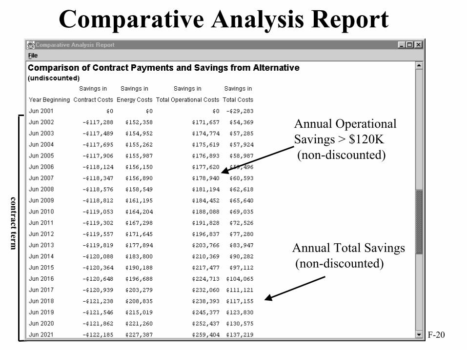
F-20

Comparative Analysis Report

contract term

Annual Operational Savings > $120K(non-discounted)

Annual Total Savings (non-discounted)

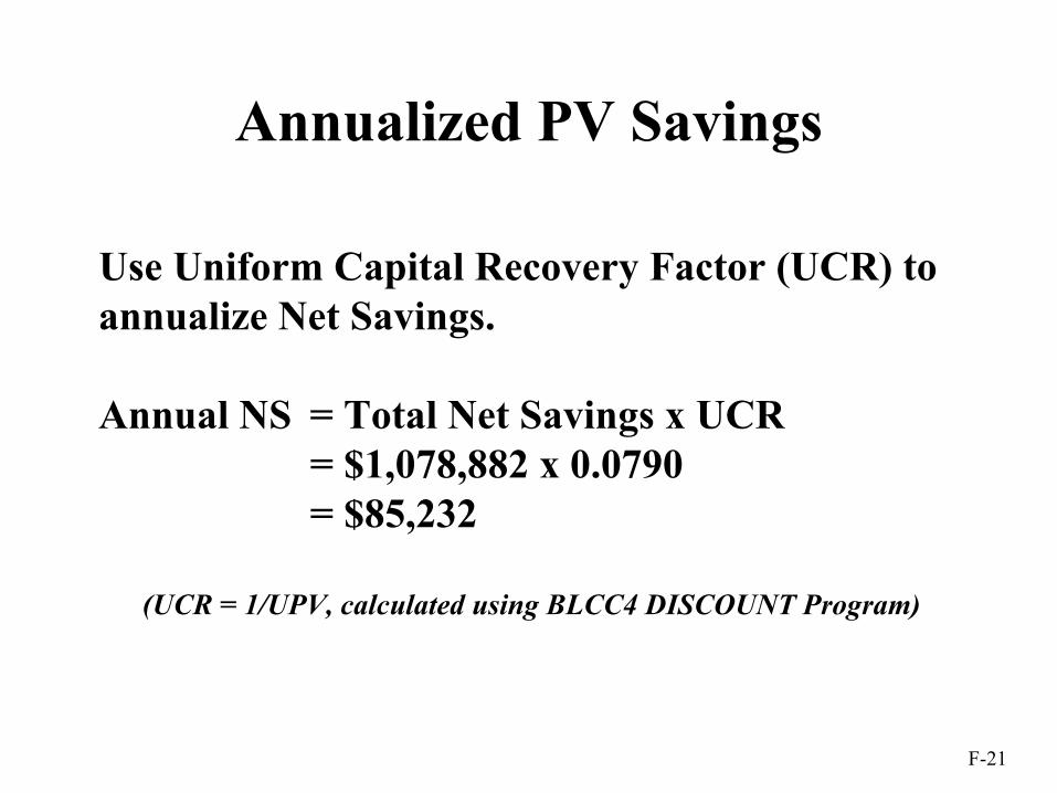
F-21

Annualized PV Savings

Use Uniform Capital Recovery Factor (UCR) to annualize Net Savings.

Annual NS = Total Net Savings x UCR= $1,078,882 x 0.0790= $85,232

(UCR = 1/UPV, calculated using BLCC4 DISCOUNT Program)

F-22

Summary LCC Report

BC: Do nothingAnnualized PV LCC

Alt: ESPCAnnualized PV LCC

Annualized PV Net Savings:$261,887 - $176,769 = $85,118

F-23

Summary of Analysis Results• ESPC project is cost-effective.

– LCC lower than for status quo (Lowest LCC Report)– positive NS for alternative (Comparative Analysis

Report)– annual non-discounted operational savings > than

contract payments (Comparative Analysis Report)– operational savings proposed by ESCO confirmed

• Other considerations:– emissions reduction achieved with ESPC project

(Comparative Analysis Report)

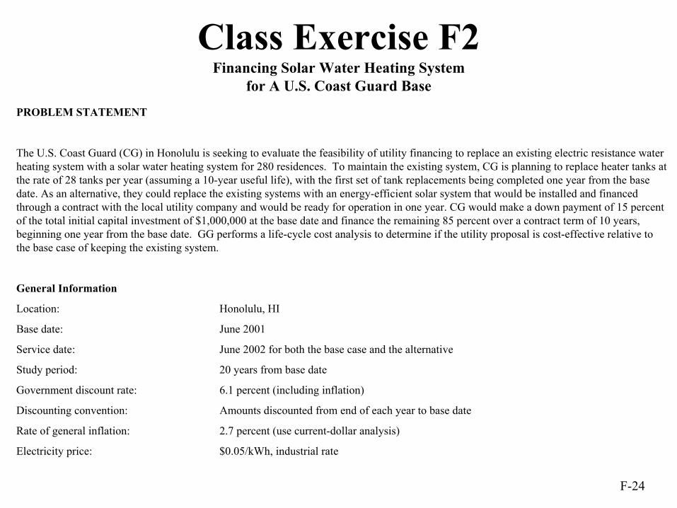
F-24

Class Exercise F2Financing Solar Water Heating System

for A U.S. Coast Guard Base

PROBLEM STATEMENT

The U.S. Coast Guard (CG) in Honolulu is seeking to evaluate the feasibility of utility financing to replace an existing electric resistance water heating system with a solar water heating system for 280 residences. To maintain the existing system, CG is planning to replace heater tanks at the rate of 28 tanks per year (assuming a 10-year useful life), with the first set of tank replacements being completed one year from the base date. As an alternative, they could replace the existing systems with an energy-efficient solar system that would be installed and financed through a contract with the local utility company and would be ready for operation in one year. CG would make a down payment of 15 percent of the total initial capital investment of $1,000,000 at the base date and finance the remaining 85 percent over a contract term of 10 years, beginning one year from the base date. GG performs a life-cycle cost analysis to determine if the utility proposal is cost-effective relative to the base case of keeping the existing system.

General Information

Location: Honolulu, HI

Base date: June 2001

Service date: June 2002 for both the base case and the alternative

Study period: 20 years from base date

Government discount rate: 6.1 percent (including inflation)

Discounting convention: Amounts discounted from end of each year to base date

Rate of general inflation: 2.7 percent (use current-dollar analysis)

Electricity price: $0.05/kWh, industrial rate

F-25

Class Exercise F2 (cont.)Base Case: Maintain and Repair Existing System

Annual electricity cost: $148,750 (= 2,975,000 kWh at $0.05)

Initial capital investment: None

Capital replacement costs:

Years 6, 11, and 16: $23,760 for anode replacements

Annually recurring OM&R costs: $32,220 for tank replacements, at the rate of 28 tanks per year, assuming a 10-year tank life

Alternative 1: Solar Water Heating System Financed through Utility Contract

Contract-related data:

Contract term: 10 years, beginning one year from base date

Loan payments: $123,833 per year during contract term, fixed

Administrative costs: $1,000 per year during contract term, increasing at the rate of inflation

Oversight costs: $1,800 at contract date

Annual electricity cost: $27,100 (= 542,000 kWh at $0.05)

Initial capital investment: $1,000,000

15% (=$150,000) down payment at base date

85% (= $850,000) financed through UC

F-26

Class Exercise F2 (cont.)Capital Replacement costs:

Year 11: $30,000 for replacing anodes and controls

Year 11: $230,400 for replacing tanks

Year 16: $18,580 for replacing valves, residual value 73%

Annually recurring OM&R costs: $7,600 for routine maintenance, included in loan

payment during contract term

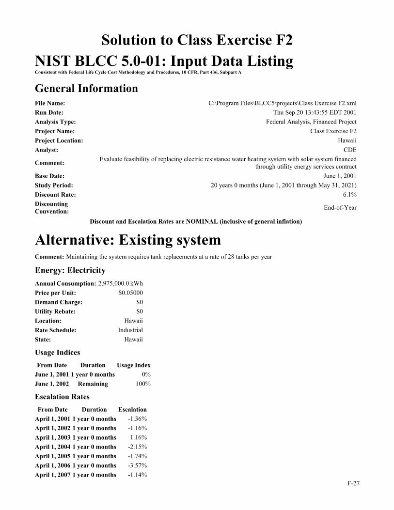
F-27

Solution to Class Exercise F2 NIST BLCC 5.0-01: Input Data Listing Consistent with Federal Life Cycle Cost Methodology and Procedures, 10 CFR, Part 436, Subpart A

General Information File Name: C:\Program Files\BLCC5\projects\Class Exercise F2.xml Run Date: Thu Sep 20 13:43:55 EDT 2001 Analysis Type: Federal Analysis, Financed Project Project Name: Class Exercise F2 Project Location: Hawaii Analyst: CDE

Comment: Evaluate feasibility of replacing electric resistance water heating system with solar system financed through utility energy services contract

Base Date: June 1, 2001 Study Period: 20 years 0 months (June 1, 2001 through May 31, 2021) Discount Rate: 6.1% Discounting Convention: End-of-Year

Discount and Escalation Rates are NOMINAL (inclusive of general inflation)

Alternative: Existing system Comment: Maintaining the system requires tank replacements at a rate of 28 tanks per year

Energy: Electricity Annual Consumption: 2,975,000.0 kWh Price per Unit: $0.05000 Demand Charge: $0 Utility Rebate: $0 Location: Hawaii Rate Schedule: Industrial State: Hawaii

Usage Indices From Date Duration Usage Index

June 1, 2001 1 year 0 months 0% June 1, 2002 Remaining 100%

Escalation Rates From Date Duration Escalation

April 1, 2001 1 year 0 months -1.36% April 1, 2002 1 year 0 months -1.16% April 1, 2003 1 year 0 months 1.16% April 1, 2004 1 year 0 months -2.15% April 1, 2005 1 year 0 months -1.74% April 1, 2006 1 year 0 months -3.57% April 1, 2007 1 year 0 months -1.14%

F-28

April 1, 2008 1 year 0 months 1.37% April 1, 2009 1 year 0 months 1.06% April 1, 2010 1 year 0 months 1.53% April 1, 2011 1 year 0 months 1.81% April 1, 2012 1 year 0 months 2.8% April 1, 2013 1 year 0 months 3.8% April 1, 2014 1 year 0 months 3% April 1, 2015 1 year 0 months 2.8% April 1, 2016 1 year 0 months 3.88% April 1, 2017 1 year 0 months 2.60% April 1, 2018 1 year 0 months 2.41% April 1, 2019 1 year 0 months 3.58% April 1, 2020 1 year 0 months 3.09% April 1, 2021 1 year 0 months 2.89% April 1, 2022 1 year 0 months 2.89% April 1, 2023 1 year 0 months 2.89% April 1, 2024 1 year 0 months 2.89% April 1, 2025 1 year 0 months 2.89% April 1, 2026 1 year 0 months 2.89% April 1, 2027 1 year 0 months 2.99% April 1, 2028 1 year 0 months 2.89% April 1, 2029 1 year 0 months 2.89% April 1, 2030 1 year 0 months 2.89% April 1, 2031 Remaining 2.91%

Component: Initial Investment Initial Cost Paid By Agency (base-year $): $0 Initial Cost Financed (base-year $): $0 Annual Rate of Increase: 2.7% Expected Asset Life: 20 years 0 months Residual Value Factor: 0%

Cost-Phasing Cost Adjustment Factor: 2.7% Years/Months (from Date) Date Portion

0 years 0 months June 1, 2001 100%

Replacement: Year 6 Anode Replacement Years/Months: 6 years 0 months Amount: $23,760 Annual Rate Of Increase: 2.7% Expected Asset Life: 5 years 0 months Residual Value Factor: 0%

Replacement: Year 11 Anode Replacement Years/Months: 11 years 0 months

F-29

Amount: $23,760 Annual Rate Of Increase: 2.7% Expected Asset Life: 5 years 0 months Residual Value Factor: 0%

Replacement: Year 16 Anode Replacement Years/Months: 16 years 0 months Amount: $23,760 Annual Rate Of Increase: 2.7% Expected Asset Life: 5 years 0 months Residual Value Factor: 20%

Recurring OM&R: Tank replacement Amount: $32,220 Annual Rate of Increase: 2.7%

Usage Indices From Date Duration Factor

June 1, 2001 1 year 0 months 0% June 1, 2002 Remaining 100%

Alternative: Solar Water Heating System Comment: 85% of the cost of the solar water heating system will be financed through a utility contract

Recurring Contract: Annual Loan Payment Amount: $123,833 Annual Rate of Increase: 0%

Usage Indices From Date Duration Factor

June 1, 2001 1 year 0 months 0% June 1, 2002 10 years 0 months 100% June 1, 2012 Remaining 0%

Recurring Contract: Administrative Costs Amount: $1,000 Annual Rate of Increase: 2.7%

Usage Indices From Date Duration Factor

June 1, 2001 1 year 0 months 0% June 1, 2002 10 years 0 months 100% June 1, 2012 Remaining 0%

Non-Recurring Contract: Oversight Cost Years/Months: 1 year 0 months Amount: $1,800 Annual Rate of Increase: 2.7%

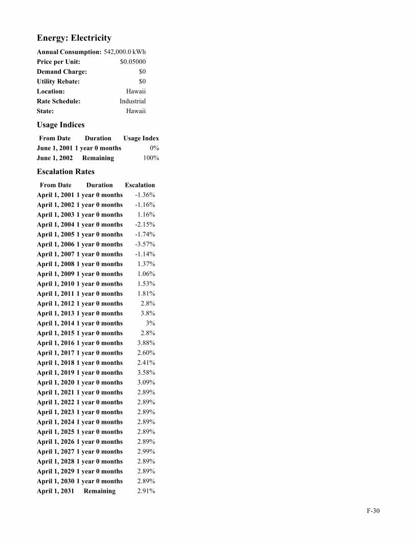
F-30

Energy: Electricity Annual Consumption: 542,000.0 kWh Price per Unit: $0.05000 Demand Charge: $0 Utility Rebate: $0 Location: Hawaii Rate Schedule: Industrial State: Hawaii

Usage Indices From Date Duration Usage Index

June 1, 2001 1 year 0 months 0% June 1, 2002 Remaining 100%

Escalation Rates From Date Duration Escalation

April 1, 2001 1 year 0 months -1.36% April 1, 2002 1 year 0 months -1.16% April 1, 2003 1 year 0 months 1.16% April 1, 2004 1 year 0 months -2.15% April 1, 2005 1 year 0 months -1.74% April 1, 2006 1 year 0 months -3.57% April 1, 2007 1 year 0 months -1.14% April 1, 2008 1 year 0 months 1.37% April 1, 2009 1 year 0 months 1.06% April 1, 2010 1 year 0 months 1.53% April 1, 2011 1 year 0 months 1.81% April 1, 2012 1 year 0 months 2.8% April 1, 2013 1 year 0 months 3.8% April 1, 2014 1 year 0 months 3% April 1, 2015 1 year 0 months 2.8% April 1, 2016 1 year 0 months 3.88% April 1, 2017 1 year 0 months 2.60% April 1, 2018 1 year 0 months 2.41% April 1, 2019 1 year 0 months 3.58% April 1, 2020 1 year 0 months 3.09% April 1, 2021 1 year 0 months 2.89% April 1, 2022 1 year 0 months 2.89% April 1, 2023 1 year 0 months 2.89% April 1, 2024 1 year 0 months 2.89% April 1, 2025 1 year 0 months 2.89% April 1, 2026 1 year 0 months 2.89% April 1, 2027 1 year 0 months 2.99% April 1, 2028 1 year 0 months 2.89% April 1, 2029 1 year 0 months 2.89% April 1, 2030 1 year 0 months 2.89% April 1, 2031 Remaining 2.91%

F-31

Component: Initial Investment Initial Cost Paid By Agency (base-year $): $150,000 Initial Cost Financed (base-year $): $850,000 Annual Rate of Increase: 2.7% Expected Asset Life: 20 years 0 months Residual Value Factor: 0%

Cost-Phasing Cost Adjustment Factor: 2.7% Years/Months (from Date) Date Portion

0 years 0 months June 1, 2001 100%

Replacement: Anodes/Controls Years/Months: 11 years 0 months Amount: $30,000 Annual Rate Of Increase: 2.7% Expected Asset Life: 10 years 0 months Residual Value Factor: 0%

Replacement: Tanks Years/Months: 11 years 0 months Amount: $230,400 Annual Rate Of Increase: 2.7% Expected Asset Life: 10 years 0 months Residual Value Factor: 0%

Replacement: Valves Years/Months: 16 years 0 months Amount: $18,580 Annual Rate Of Increase: 2.7% Expected Asset Life: 15 years 0 months Residual Value Factor: 73%

Recurring OM&R: Routine OM&R Amount: $7,600 Annual Rate of Increase: 2.7%

Usage Indices From Date Duration Factor

June 1, 2001 11 years 0 months 0% June 1, 2012 Remaining 100%

F-32

NIST BLCC 5.0-01: Detailed LCC Analysis Consistent with Federal Life Cycle Cost Methodology and Procedures, 10 CFR, Part 436, Subpart A

General Information File Name: C:\Program Files\BLCC5\projects\Class Exercise F2.xml Run Date: Thu Sep 20 13:46:39 EDT 2001 Analysis Type: Federal Analysis, Financed Project Project Name: Class Exercise F2 Project Location: Hawaii Analyst: CDE

Comment: Evaluate feasibility of replacing electric resistance water heating system with solar system financed through utility energy services contract

Base Date: June 1, 2001 Study Period: 20 years 0 months (June 1, 2001 through May 31, 2021) Discount Rate: 6.1% Discounting Convention: End-of-Year

Discount and Escalation Rates are NOMINAL (inclusive of general inflation)

Alternative: Existing system Initial Cost Data (not Discounted) Initial Capital Costs Paid By Agency (adjusted for price escalation)

Initial Capital Costs for All Components: $0

Component: Cost-Phasing

Date Portion Yearly Cost June 1, 2001 100% $0

------------ ------------

Total (for Component) $0

Initial Capital Costs Financed (base-year dollars)

Initial Capital Costs for All Components: $0

Component: Initial Cost Financed $0

Energy Costs: Electricity (base-year dollars)

Average Average Average Average Annual Usage Price/Unit Annual Cost Annual Demand Annual Rebate

2,826,331.5 kWh $0.05000 $141,317 $0 $0

Life-Cycle Cost Analysis

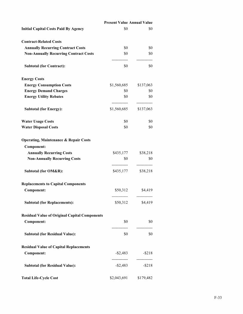
F-33

Present Value Annual Value Initial Capital Costs Paid By Agency $0 $0

Contract-Related Costs Annually Recurring Contract Costs $0 $0 Non-Annually Recurring Contract Costs $0 $0

------------ ------------ Subtotal (for Contract): $0 $0

Energy Costs Energy Consumption Costs $1,560,685 $137,063 Energy Demand Charges $0 $0 Energy Utility Rebates $0 $0

------------ ------------ Subtotal (for Energy): $1,560,685 $137,063

Water Usage Costs $0 $0 Water Disposal Costs $0 $0

Operating, Maintenance & Repair Costs Component: Annually Recurring Costs $435,177 $38,218 Non-Annually Recurring Costs $0 $0

------------ ------------ Subtotal (for OM&R): $435,177 $38,218

Replacements to Capital Components Component: $50,312 $4,419

------------ ------------ Subtotal (for Replacements): $50,312 $4,419

Residual Value of Original Capital Components Component: $0 $0

------------ ------------ Subtotal (for Residual Value): $0 $0

Residual Value of Capital Replacements Component: -$2,483 -$218

------------ ------------ Subtotal (for Residual Value): -$2,483 -$218

Total Life-Cycle Cost $2,043,691 $179,482

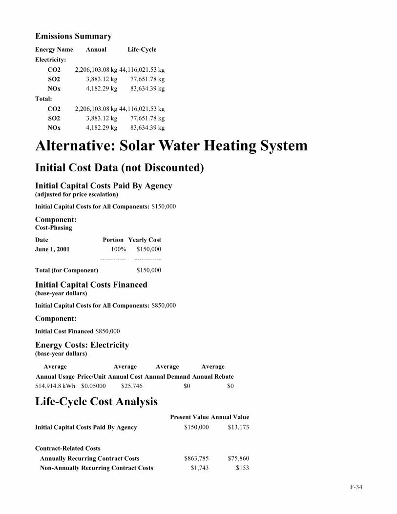
F-34

Emissions Summary Energy Name Annual Life-Cycle Electricity:

CO2 2,206,103.08 kg 44,116,021.53 kg SO2 3,883.12 kg 77,651.78 kg NOx 4,182.29 kg 83,634.39 kg

Total: CO2 2,206,103.08 kg 44,116,021.53 kg SO2 3,883.12 kg 77,651.78 kg NOx 4,182.29 kg 83,634.39 kg

Alternative: Solar Water Heating System Initial Cost Data (not Discounted) Initial Capital Costs Paid By Agency (adjusted for price escalation)

Initial Capital Costs for All Components: $150,000

Component: Cost-Phasing Date Portion Yearly Cost June 1, 2001 100% $150,000

------------ ------------

Total (for Component) $150,000

Initial Capital Costs Financed (base-year dollars)

Initial Capital Costs for All Components: $850,000

Component: Initial Cost Financed $850,000

Energy Costs: Electricity (base-year dollars)

Average Average Average Average Annual Usage Price/Unit Annual Cost Annual Demand Annual Rebate 514,914.8 kWh $0.05000 $25,746 $0 $0

Life-Cycle Cost Analysis Present Value Annual Value Initial Capital Costs Paid By Agency $150,000 $13,173

Contract-Related Costs Annually Recurring Contract Costs $863,785 $75,860 Non-Annually Recurring Contract Costs $1,743 $153

F-35

------------ ------------ Subtotal (for Contract): $865,527 $76,013

Energy Costs Energy Consumption Costs $284,333 $24,971 Energy Demand Charges $0 $0 Energy Utility Rebates $0 $0

------------ ------------ Subtotal (for Energy): $284,333 $24,971

Water Usage Costs $0 $0 Water Disposal Costs $0 $0

Operating, Maintenance & Repair Costs Component: Annually Recurring Costs $40,834 $3,586 Non-Annually Recurring Costs $0 $0

------------ ------------ Subtotal (for OM&R): $40,834 $3,586

Replacements to Capital Components Component: $193,243 $16,971

------------ ------------ Subtotal (for Replacements): $193,243 $16,971

Residual Value of Original Capital Components Component: $0 $0

------------ ------------ Subtotal (for Residual Value): $0 $0

Residual Value of Capital Replacements Component: -$7,086 -$622

------------ ------------ Subtotal (for Residual Value): -$7,086 -$622

Total Life-Cycle Cost $1,526,852 $134,092

F-36

Emissions Summary Energy Name Annual Life-Cycle Electricity:

CO2 401,918.61 kg 8,037,271.82 kg SO2 707.45 kg 14,146.98 kg NOx 761.95 kg 15,236.92 kg

Total: CO2 401,918.61 kg 8,037,271.82 kg SO2 707.45 kg 14,146.98 kg NOx 761.95 kg 15,236.92 kg

F-37

NIST BLCC 5.0-01: Comparative Analysis Consistent with Federal Life Cycle Cost Methodology and Procedures, 10 CFR, Part 436, Subpart A

Base Case: Existing system Alternative: Solar Water Heating System

General Information File Name: C:\Program Files\BLCC5\projects\Class Exercise F2.xml Run Date: Thu Sep 20 13:52:25 EDT 2001 Project Name: Class Exercise F2 Project Location: Hawaii Analysis Type: Federal Analysis, Financed Project Analyst: CDE

Comment Evaluate feasibility of replacing electric resistance water heating system with solar system financed through utility energy services contract

Base Date of Study: June 1, 2001 Service Date: June 1, 2001 Study Period: 20 years 0 months(June 1, 2001 through May 31, 2021) Discount Rate: 6.1% Discounting Convention: End-of-Year

Comparison of Present-Value Costs PV Life-Cycle Cost Base Case Alternative Savings from Alternative

Initial Investment Costs Paid By Agency: Capital Requirements as of Base Date $0 $150,000 -$150,000 Future Costs: Recurring and Non-Recurring Contract Costs $0 $865,527 -$865,527 Energy Consumption Costs $1,560,685 $284,333 $1,276,352 Energy Demand Charges $0 $0 $0 Energy Utility Rebates $0 $0 $0 Water Costs $0 $0 $0 Recurring and Non-Recurring OM&R Costs $435,177 $40,834 $394,343 Capital Replacements $50,312 $193,243 -$142,931 Residual Value at End of Study Period -$2,483 -$7,086 $4,603

------------ ------------ ------------ Subtotal (for Future Cost Items) $2,043,691 $1,376,852 $666,840

------------ ------------ ------------ Total PV Life-Cycle Cost $2,043,691 $1,526,852 $516,840

Net Savings from Alternative Compared with Base Case PV of Operational Savings $1,670,694

F-38

- PV of Differential Costs $1,153,855

------------ Net Savings $516,840

NOTE: Meaningful SIR, AIRR and Payback can not be computed for Financed Projects.

Comparison of Contract Payments and Savings from Alternative (undiscounted)

Savings in Savings in Savings in Savings in Year Beginning Contract Costs Energy Costs Total Operational Costs Total Costs Jun 2001 $0 $0 $0 -$150,000 Jun 2002 -$126,736 $119,101 $153,081 $26,345 Jun 2003 -$124,916 $119,827 $154,726 $29,810 Jun 2004 -$124,945 $117,330 $153,171 $28,225 Jun 2005 -$124,975 $114,938 $151,746 $26,771 Jun 2006 -$125,006 $111,293 $149,094 $24,087 Jun 2007 -$125,038 $110,474 $149,298 $52,137 Jun 2008 -$125,070 $111,931 $151,802 $26,732 Jun 2009 -$125,104 $113,206 $154,153 $29,049 Jun 2010 -$125,138 $114,985 $157,037 $31,898 Jun 2011 -$125,173 $117,256 $160,445 $35,272 Jun 2012 $0 $120,728 $154,620 -$162,607 Jun 2013 $0 $125,149 $159,956 $159,956 Jun 2014 $0 $128,856 $164,601 $164,601 Jun 2015 $0 $132,697 $169,410 $169,410 Jun 2016 $0 $137,561 $175,265 $175,265 Jun 2017 $0 $141,095 $179,816 $187,750 Jun 2018 $0 $144,760 $184,526 $184,526 Jun 2019 $0 $149,834 $190,675 $190,675 Jun 2020 $0 $154,396 $196,336 $211,347

Energy Savings Summary Energy Savings Summary (in stated units) Energy -----Average Annual Consumption----- Life-Cycle Type Base Case Alternative Savings Savings Electricity 2,826,331.5 kWh 514,914.8 kWh 2,311,416.6 kWh 46,222,004.1 kWh

Energy Savings Summary (in MBtu) Energy -----Average Annual Consumption----- Life-Cycle Type Base Case Alternative Savings Savings Electricity 9,643.8 MBtu 1,757.0 MBtu 7,886.9 MBtu 157,716.0 MBtu

F-39

Emissions Reduction Summary Energy -----Average Annual Emissions----- Life-Cycle Type Base Case Alternative Reduction Reduction Electricity

CO2 2,206,103.08 kg 401,918.61 kg 1,804,184.46 kg 36,078,749.71 kg SO2 3,883.12 kg 707.45 kg 3,175.67 kg 63,504.80 kg NOx 4,182.29 kg 761.95 kg 3,420.34 kg 68,397.47 kg

Total: CO2 2,206,103.08 kg 401,918.61 kg 1,804,184.46 kg 36,078,749.71 kg SO2 3,883.12 kg 707.45 kg 3,175.67 kg 63,504.80 kg NOx 4,182.29 kg 761.95 kg 3,420.34 kg 68,397.47 kg

G-1

Module GClass Exercises

G-2

Class Exercise G1Water Conservation

A military barracks at Fort Meade, MD, housing 200 enlisted men, uses 800,000 gallons of water peryear at a cost of $4.00/1000 gallons of use plus $5.00/1000 gallons sewer charge. This barracks isscheduled to be replaced with a new barracks in seven years. A water conservation project is proposedthat will reduce usage and disposal by 25 % at an initial cost of $5,000 and which will not havemaintenance costs over the seven years of remaining building life. All of the project components have alife expectancy of seven years or more. Water usage and disposal prices are expected to increase by anaverage of 5 %/year over general inflation for the remaining life of the building. During the last twoyears of the barracks’ life, the occupancy level (and thus water consumption) is expected to be half of thecurrent level.

The base date and service date are specified as June 2001. Use the mid-year discounting convention.

Using BLCC5, compute the life-cycle water-related costs before and after the retrofit project. ComputeNet Savings and Savings-to-Investment Ratio. Would you recommend this project be undertaken?

G-3

Class Exercise G2Chiller Replacement

As energy manager of a federal research facility, you are tasked with replacing the existing 1000-tonchiller, which has an expected remaining life of 10 years but must be replaced to eliminate CFC usage.You have submitted technical specifications and operating conditions to all large chiller manufacturersand asked for bid responses which are to include the following cost and energy-related data: first cost,annual energy costs based on current electricity costs, and the operating schedule that you submit. Themanufacturers must calculate annual energy usage and peak energy usage for their system using astandardized energy-estimating method. You inform the manufacturers that you will select the bid withthe lowest 25-year life-cycle cost, using current FEMP LCC criteria (3.3 % discount rate and DOEescalation rates (South (Texas), industrial rates) and the BLCC computer program to perform the LCCcalculations. Since you expect that maintenance costs after the end of the 10-year service contract willbe similar for all systems, O&M costs can be ignored after year 10. Current electricity costs are$.048/kWh for electricity usage (same during winter and summer) and $104/kW-y demand charge forpeak kW demand. (Multiply the maximum annual kW demand by $104 to get the annual demandcharge.) Water costs and other operating costs are assumed to be similar for all systems for the purposeof this competition. The base date and service date for all LCC analyses are specified as June 2001. Usethe end-of-year discounting convention.

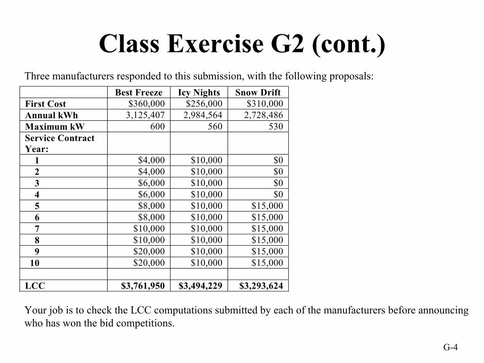
G-4

Class Exercise G2 (cont.)Three manufacturers responded to this submission, with the following proposals: Best Freeze Icy Nights Snow Drift First Cost $360,000 $256,000 $310,000 Annual kWh 3,125,407 2,984,564 2,728,486 Maximum kW 600 560 530 Service Contract Year:

1 $4,000 $10,000 $0 2 $4,000 $10,000 $0 3 $6,000 $10,000 $0 4 $6,000 $10,000 $0 5 $8,000 $10,000 $15,000 6 $8,000 $10,000 $15,000 7 $10,000 $10,000 $15,000 8 $10,000 $10,000 $15,000 9 $20,000 $10,000 $15,000 10 $20,000 $10,000 $15,000 LCC $3,761,950 $3,494,229 $3,293,624 Your job is to check the LCC computations submitted by each of the manufacturers before announcing who has won the bid competitions.

G-5

Class Exercise G3Alternative Financing of Energy Conservation Project

A federal agency in Arizona is considering replacing an existing lighting system in an office building with a new lighting/daylighting system financed through a utility contract. The existing lighting system is expected to be operational for another 15 years. Use BLCC5 to perform an LCC analysis.

Project Information

Location: Arizona

Base Date: June 2001

Study Period: 15 years

Contract Term: 10 years

Discount Rate: 6.1%

Annual Rate of Inflation: 2.7%

Discounting Convention: end-of-year

G-6

Class Exercise G3 (cont.)Base Case

Initial Investment Cost: 0

Energy Type: Electricity

Annual Usage: 1,082,633 kWh

Price: $0.04600/kWh, commercial

Annual Demand Charge: $30,105

Annual OM&R costs: $5,600

Alternative

Amount Borrowed: $390,480

Expected Life: 20 years

Residual Value Factor: 25%

Annual Contract Payment: $62,000, fixed

Energy Type: Electricity

Annual Usage: 206,911 kWh

Price: $0.04600/kWh, commercial

Annual Demand Charge: $3,311

Annual OM&R: $0 during contract term

$3,000 in years 11 through 15

G-7

Class Exercise G4Lease Versus Buy Decision (BLCC4 Exercise)

A federal government agency is considering building a new office building with 60,000 square feet of office space on land that it already owns at an initial cost of $5,000,000. A private investment firm offers to build the same building on private land across the street from the proposed site and lease this facility to the government for 20 years at an annual lease rate of $500,000, with an annual escalation clause that is tied directly to the rate of general inflation. Major building maintenance, which will cost the government $200,000 per year at current prices, is included in the lease amount. All utility costs and other building operating-related costs will be the same for both buildings. The building has an expected life of 50 years and a residual value at the end of the study period equal to 50% of its initial cost, in constant dollar terms. Which alternative is more advantageous to the government?

Use the Federal Analysis--Projects Subject to OMB A-94 Module in BLCC4. June 2001 should be used for the base date and service date. Use the end-of-year discounting convention. The projected annual rate of general inflation is 2.7%. Can this analysis be performed in constant dollars?

G-8

Solution to Class Exercise G1 NIST BLCC 5.0-01: Input Data Listing Consistent with Federal Life Cycle Cost Methodology and Procedures, 10 CFR, Part 436, Subpart A

General Information File Name: C:\Program Files\BLCC5\projects\Class Exercise

G1.xml Run Date: Thu Sep 20 14:08:19 EDT 2001 Analysis Type: Federal Analysis, Agency-Funded Project Project Name: Class Exercise G1 Project Location: Maryland Analyst: ASR Comment: Military Barracks at Fort Meade, MD Base Date: June 1, 2001 Service Date: June 1, 2001 Study Period: 7 years 0 months (June 1, 2001 through May 31, 2008) Discount Rate: 3.3% Discounting Convention: Mid-Year

Discount and Escalation Rates are REAL (exclusive of general inflation)

Alternative: Existing Water: Water Annual Usage Annual Disposal Units/Year Price/Unit Units/Year Price/Unit @Summer Rates 800.0 ThousGal $4.00000 800.0 ThousGal $5.00000 @Winter Rates 0.0 ThousGal $0.00000 0.0 ThousGal $0.00000

Escalation Rates - Usage From Date Duration Usage Cost Escalation

June 1, 2001 Remaining 5.00%

Escalation Rates - Disposal From Date Duration Disposal Cost Escalation

June 1, 2001 Remaining 5.00%

Usage Indices - Usage From Date Duration Index

June 1, 2001 5 years 0 months 100% June 1, 2006 Remaining 50%

G-9

Usage Indices - Disposal From Date Duration Index

June 1, 2001 5 years 0 months 100% June 1, 2006 Remaining 50%

Component: Initial Investment Initial Cost (base-year $): $0 Annual Rate of Increase: 0% Expected Asset Life: 0 years 0 months Residual Value Factor: 0%

Cost-Phasing Cost Adjustment Factor: 0% Years/Months (from Date) Date Portion

0 years 0 months June 1, 2001 100%

Alternative: Water Project Water: Water Annual Usage Annual Disposal Units/Year Price/Unit Units/Year Price/Unit @Summer Rates 600.0 ThousGal $4.00000 600.0 ThousGal $5.00000 @Winter Rates 0.0 ThousGal $0.00000 0.0 ThousGal $0.00000

Escalation Rates - Usage From Date Duration Usage Cost Escalation

June 1, 2001 Remaining 5.00%

Escalation Rates - Disposal From Date Duration Disposal Cost Escalation

June 1, 2001 Remaining 5.00%

Usage Indices - Usage From Date Duration Index

June 1, 2001 5 years 0 months 100% June 1, 2006 Remaining 50%

Usage Indices - Disposal From Date Duration Index

June 1, 2001 5 years 0 months 100% June 1, 2006 Remaining 50%

Component: Initial Investment Initial Cost (base-year $): $5,000

G-10

Annual Rate of Increase: 0% Expected Asset Life: 7 years 0 months Residual Value Factor: 0%

Cost-Phasing Cost Adjustment Factor: 0% Years/Months (from Date) Date Portion

0 years 0 months June 1, 2001 100%

G-11

NIST BLCC 5.0-01: Comparative Analysis Consistent with Federal Life Cycle Cost Methodology and Procedures, 10 CFR, Part 436, Subpart A

Base Case: Existing Alternative: Water Project

General Information File Name: C:\Program Files\BLCC5\projects\Class Exercise G1.xml Run Date: Thu Sep 20 14:10:47 EDT 2001 Project Name: Class Exercise G1 Project Location: Maryland Analysis Type: Federal Analysis, Agency-Funded Project Analyst: ASR Comment Military Barracks at Fort Meade, MD Base Date of Study: June 1, 2001 Service Date: June 1, 2001 Study Period: 7 years 0 months(June 1, 2001 through May 31, 2008) Discount Rate: 3.3% Discounting Convention: Mid-Year

Comparison of Present-Value Costs PV Life-Cycle Cost Base Case Alternative Savings from Alternative

Initial Investment Costs: Capital Requirements as of Base Date $0 $5,000 -$5,000 Future Costs: Energy Consumption Costs $0 $0 $0 Energy Demand Charges $0 $0 $0 Energy Utility Rebates $0 $0 $0 Water Costs $45,450 $34,088 $11,363 Recurring and Non-Recurring OM&R Costs $0 $0 $0 Capital Replacements $0 $0 $0 Residual Value at End of Study Period $0 $0 $0

------------ ------------ ------------ Subtotal (for Future Cost Items) $45,450 $34,088 $11,363

------------ ------------ ------------ Total PV Life-Cycle Cost $45,450 $39,088 $6,363

Net Savings from Alternative Compared with Base Case PV of Non-Investment Savings $11,363 - Increased Total Investment $5,000

------------ Net Savings $6,363

G-12

Savings-to-Investment Ratio (SIR) SIR = 2.27

Adjusted Internal Rate of Return AIRR = 16.16%

Payback Period Estimated Years to Payback (from beginning of Service Period) Simple Payback occurs in year 3 Discounted Payback occurs in year 3

G-13

Solution to Class Exercise G2 NIST BLCC 5.0-01: Input Data Listing Consistent with Federal Life Cycle Cost Methodology and Procedures, 10 CFR, Part 436, Subpart A

General Information File Name: C:\Program Files\BLCC5\projects\Class Exercise

G2.xml Run Date: Thu Sep 20 14:23:51 EDT 2001 Analysis Type: Federal Analysis, Agency-Funded Project Project Name: Class Exercise G2 Project Location: Texas Analyst: ASR Base Date: June 1, 2001 Service Date: June 1, 2001 Study Period: 25 years 0 months (June 1, 2001 through May 31, 2026) Discount Rate: 3.3% Discounting Convention: End-of-Year

Discount and Escalation Rates are REAL (exclusive of general inflation)

Alternative: Best Freeze Energy: Electricity Annual Consumption: 3,125,407.0 kWh Price per Unit: $0.04800 Demand Charge: $62,400 Utility Rebate: $0 Location: Texas Rate Schedule: Industrial State: Texas

Usage Indices From Date Duration Usage Index

June 1, 2001 Remaining 100%

Escalation Rates From Date Duration Escalation

April 1, 2001 1 year 0 months -1.99% April 1, 2002 1 year 0 months -1.22% April 1, 2003 1 year 0 months -0.25% April 1, 2004 1 year 0 months -1.32% April 1, 2005 1 year 0 months -1.09% April 1, 2006 1 year 0 months -1.52% April 1, 2007 1 year 0 months -1.2% April 1, 2008 1 year 0 months -0.87% April 1, 2009 1 year 0 months -0.35%

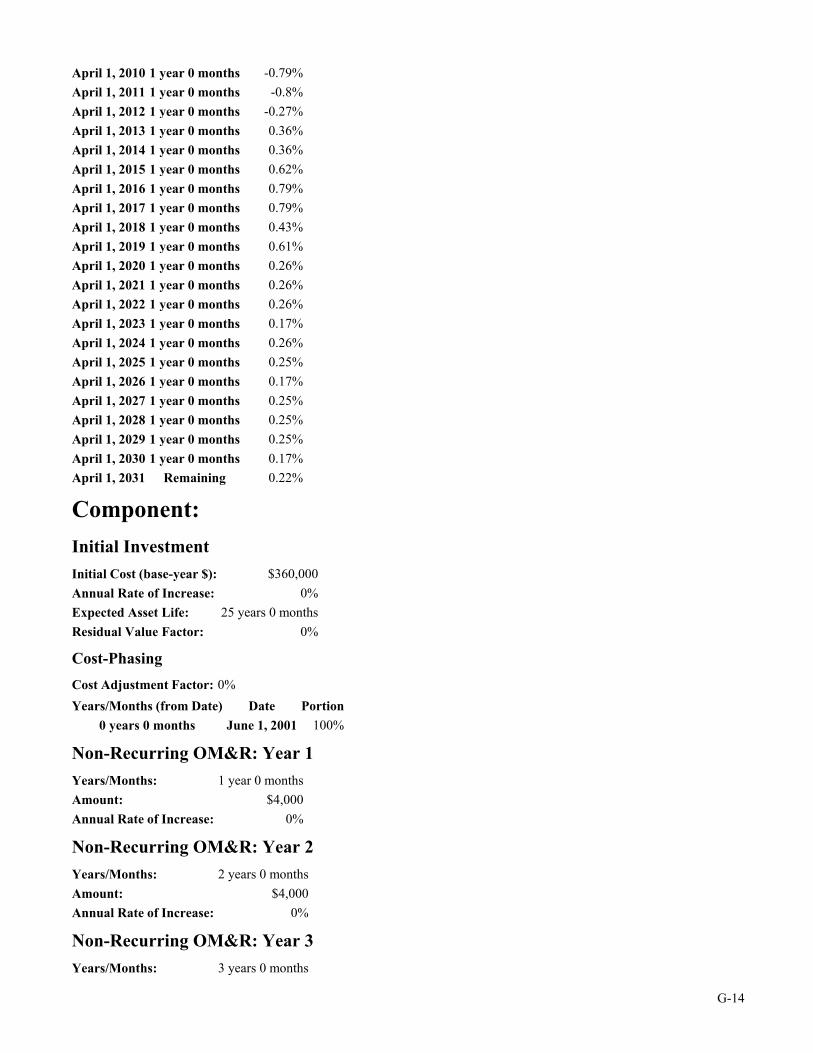
G-14

April 1, 2010 1 year 0 months -0.79% April 1, 2011 1 year 0 months -0.8% April 1, 2012 1 year 0 months -0.27% April 1, 2013 1 year 0 months 0.36% April 1, 2014 1 year 0 months 0.36% April 1, 2015 1 year 0 months 0.62% April 1, 2016 1 year 0 months 0.79% April 1, 2017 1 year 0 months 0.79% April 1, 2018 1 year 0 months 0.43% April 1, 2019 1 year 0 months 0.61% April 1, 2020 1 year 0 months 0.26% April 1, 2021 1 year 0 months 0.26% April 1, 2022 1 year 0 months 0.26% April 1, 2023 1 year 0 months 0.17% April 1, 2024 1 year 0 months 0.26% April 1, 2025 1 year 0 months 0.25% April 1, 2026 1 year 0 months 0.17% April 1, 2027 1 year 0 months 0.25% April 1, 2028 1 year 0 months 0.25% April 1, 2029 1 year 0 months 0.25% April 1, 2030 1 year 0 months 0.17% April 1, 2031 Remaining 0.22%

Component: Initial Investment Initial Cost (base-year $): $360,000 Annual Rate of Increase: 0% Expected Asset Life: 25 years 0 months Residual Value Factor: 0%

Cost-Phasing Cost Adjustment Factor: 0% Years/Months (from Date) Date Portion

0 years 0 months June 1, 2001 100%

Non-Recurring OM&R: Year 1 Years/Months: 1 year 0 months Amount: $4,000 Annual Rate of Increase: 0%

Non-Recurring OM&R: Year 2 Years/Months: 2 years 0 months Amount: $4,000 Annual Rate of Increase: 0%

Non-Recurring OM&R: Year 3 Years/Months: 3 years 0 months

G-15

Amount: $6,000 Annual Rate of Increase: 0%

Non-Recurring OM&R: Year 4 Years/Months: 4 years 0 months Amount: $6,000 Annual Rate of Increase: 0%

Non-Recurring OM&R: Year 5 Years/Months: 5 years 0 months Amount: $8,000 Annual Rate of Increase: 0%

Non-Recurring OM&R: Year 6 Years/Months: 6 years 0 months Amount: $8,000 Annual Rate of Increase: 0%

Non-Recurring OM&R: Year 7 Years/Months: 7 years 0 months Amount: $10,000 Annual Rate of Increase: 0%

Non-Recurring OM&R: Year 8 Years/Months: 8 years 0 months Amount: $10,000 Annual Rate of Increase: 0%

Non-Recurring OM&R: Year 9 Years/Months: 9 years 0 months Amount: $20,000 Annual Rate of Increase: 0%

Non-Recurring OM&R: Year 10 Years/Months: 10 years 0 months Amount: $20,000 Annual Rate of Increase: 0%

Alternative: Icy Nights Energy: Electricity Annual Consumption: 2,984,564.0 kWh Price per Unit: $0.04800 Demand Charge: $58,240 Utility Rebate: $0 Location: Texas Rate Schedule: Industrial State: Texas

G-16

Usage Indices From Date Duration Usage Index

June 1, 2001 Remaining 100%

Escalation Rates From Date Duration Escalation

April 1, 2001 1 year 0 months -1.99% April 1, 2002 1 year 0 months -1.22% April 1, 2003 1 year 0 months -0.25% April 1, 2004 1 year 0 months -1.32% April 1, 2005 1 year 0 months -1.09% April 1, 2006 1 year 0 months -1.52% April 1, 2007 1 year 0 months -1.2% April 1, 2008 1 year 0 months -0.87% April 1, 2009 1 year 0 months -0.35% April 1, 2010 1 year 0 months -0.79% April 1, 2011 1 year 0 months -0.8% April 1, 2012 1 year 0 months -0.27% April 1, 2013 1 year 0 months 0.36% April 1, 2014 1 year 0 months 0.36% April 1, 2015 1 year 0 months 0.62% April 1, 2016 1 year 0 months 0.79% April 1, 2017 1 year 0 months 0.79% April 1, 2018 1 year 0 months 0.43% April 1, 2019 1 year 0 months 0.61% April 1, 2020 1 year 0 months 0.26% April 1, 2021 1 year 0 months 0.26% April 1, 2022 1 year 0 months 0.26% April 1, 2023 1 year 0 months 0.17% April 1, 2024 1 year 0 months 0.26% April 1, 2025 1 year 0 months 0.25% April 1, 2026 1 year 0 months 0.17% April 1, 2027 1 year 0 months 0.25% April 1, 2028 1 year 0 months 0.25% April 1, 2029 1 year 0 months 0.25% April 1, 2030 1 year 0 months 0.17% April 1, 2031 Remaining 0.22%

Component: Initial Investment Initial Cost (base-year $): $256,000 Annual Rate of Increase: 0% Expected Asset Life: 25 years 0 months Residual Value Factor: 0%

Cost-Phasing Cost Adjustment Factor: 0%

G-17

Years/Months (from Date) Date Portion 0 years 0 months June 1, 2001 100%

Non-Recurring OM&R: Year 1 Years/Months: 1 year 0 months Amount: $10,000 Annual Rate of Increase: 0%

Non-Recurring OM&R: Year 2 Years/Months: 2 years 0 months Amount: $10,000 Annual Rate of Increase: 0%

Non-Recurring OM&R: Year 3 Years/Months: 3 years 0 months Amount: $10,000 Annual Rate of Increase: 0%

Non-Recurring OM&R: Year 4 Years/Months: 4 years 0 months Amount: $10,000 Annual Rate of Increase: 0%

Non-Recurring OM&R: Year 5 Years/Months: 5 years 0 months Amount: $10,000 Annual Rate of Increase: 0%

Non-Recurring OM&R: Year 6 Years/Months: 6 years 0 months Amount: $10,000 Annual Rate of Increase: 0%

Non-Recurring OM&R: Year 7 Years/Months: 7 years 0 months Amount: $10,000 Annual Rate of Increase: 0%

Non-Recurring OM&R: Year 8 Years/Months: 8 years 0 months Amount: $10,000 Annual Rate of Increase: 0%

Non-Recurring OM&R: Year 9 Years/Months: 9 years 0 months Amount: $10,000 Annual Rate of Increase: 0%

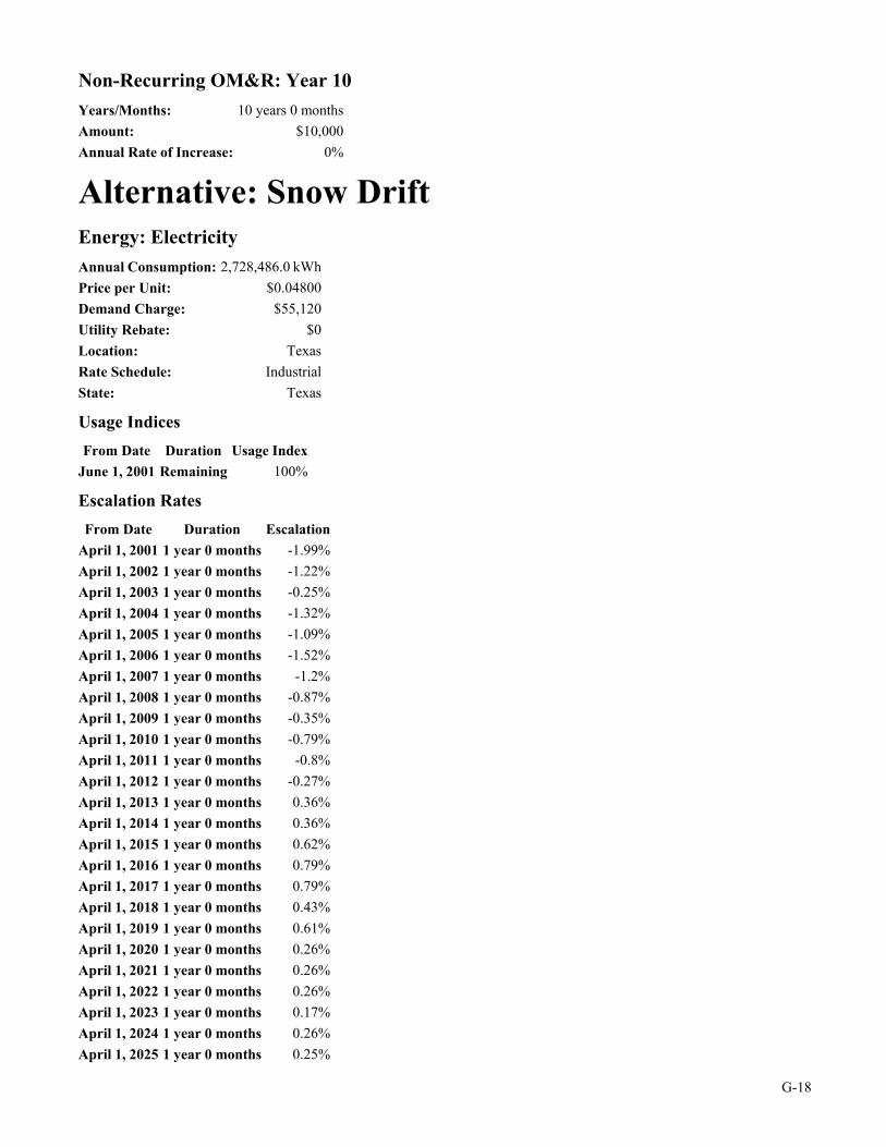
G-18

Non-Recurring OM&R: Year 10 Years/Months: 10 years 0 months Amount: $10,000 Annual Rate of Increase: 0%

Alternative: Snow Drift Energy: Electricity Annual Consumption: 2,728,486.0 kWh Price per Unit: $0.04800 Demand Charge: $55,120 Utility Rebate: $0 Location: Texas Rate Schedule: Industrial State: Texas

Usage Indices From Date Duration Usage Index

June 1, 2001 Remaining 100%

Escalation Rates From Date Duration Escalation

April 1, 2001 1 year 0 months -1.99% April 1, 2002 1 year 0 months -1.22% April 1, 2003 1 year 0 months -0.25% April 1, 2004 1 year 0 months -1.32% April 1, 2005 1 year 0 months -1.09% April 1, 2006 1 year 0 months -1.52% April 1, 2007 1 year 0 months -1.2% April 1, 2008 1 year 0 months -0.87% April 1, 2009 1 year 0 months -0.35% April 1, 2010 1 year 0 months -0.79% April 1, 2011 1 year 0 months -0.8% April 1, 2012 1 year 0 months -0.27% April 1, 2013 1 year 0 months 0.36% April 1, 2014 1 year 0 months 0.36% April 1, 2015 1 year 0 months 0.62% April 1, 2016 1 year 0 months 0.79% April 1, 2017 1 year 0 months 0.79% April 1, 2018 1 year 0 months 0.43% April 1, 2019 1 year 0 months 0.61% April 1, 2020 1 year 0 months 0.26% April 1, 2021 1 year 0 months 0.26% April 1, 2022 1 year 0 months 0.26% April 1, 2023 1 year 0 months 0.17% April 1, 2024 1 year 0 months 0.26% April 1, 2025 1 year 0 months 0.25%

G-19

April 1, 2026 1 year 0 months 0.17% April 1, 2027 1 year 0 months 0.25% April 1, 2028 1 year 0 months 0.25% April 1, 2029 1 year 0 months 0.25% April 1, 2030 1 year 0 months 0.17% April 1, 2031 Remaining 0.22%

Component: Initial Investment Initial Cost (base-year $): $310,000 Annual Rate of Increase: 0% Expected Asset Life: 25 years 0 months Residual Value Factor: 0%

Cost-Phasing Cost Adjustment Factor: 0% Years/Months (from Date) Date Portion

0 years 0 months June 1, 2001 100%

Non-Recurring OM&R: Year 1 Years/Months: 1 year 0 months Amount: $0 Annual Rate of Increase: 0%

Non-Recurring OM&R: Year 2 Years/Months: 2 years 0 months Amount: $0 Annual Rate of Increase: 0%

Non-Recurring OM&R: Year 3 Years/Months: 3 years 0 months Amount: $0 Annual Rate of Increase: 0%

Non-Recurring OM&R: Year 4 Years/Months: 4 years 0 months Amount: $0 Annual Rate of Increase: 0%

Non-Recurring OM&R: Year 5 Years/Months: 5 years 0 months Amount: $15,000 Annual Rate of Increase: 0%

Non-Recurring OM&R: Year 6 Years/Months: 6 years 0 months Amount: $15,000 Annual Rate of Increase: 0%

G-20

Non-Recurring OM&R: Year 7 Years/Months: 7 years 0 months Amount: $15,000 Annual Rate of Increase: 0%

Non-Recurring OM&R: Year 8 Years/Months: 8 years 0 months Amount: $15,000 Annual Rate of Increase: 0%

Non-Recurring OM&R: Year 9 Years/Months: 9 years 0 months Amount: $15,000 Annual Rate of Increase: 0%

Non-Recurring OM&R: Year 10 Years/Months: 10 years 0 months Amount: $15,000 Annual Rate of Increase: 0%

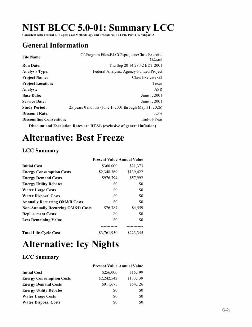
G-21

NIST BLCC 5.0-01: Summary LCC Consistent with Federal Life Cycle Cost Methodology and Procedures, 10 CFR, Part 436, Subpart A

General Information File Name: C:\Program Files\BLCC5\projects\Class Exercise

G2.xml Run Date: Thu Sep 20 14:28:42 EDT 2001 Analysis Type: Federal Analysis, Agency-Funded Project Project Name: Class Exercise G2 Project Location: Texas Analyst: ASR Base Date: June 1, 2001 Service Date: June 1, 2001 Study Period: 25 years 0 months (June 1, 2001 through May 31, 2026) Discount Rate: 3.3% Discounting Convention: End-of-Year

Discount and Escalation Rates are REAL (exclusive of general inflation)

Alternative: Best Freeze LCC Summary Present Value Annual Value Initial Cost $360,000 $21,373 Energy Consumption Costs $2,348,369 $139,422 Energy Demand Costs $976,794 $57,992 Energy Utility Rebates $0 $0 Water Usage Costs $0 $0 Water Disposal Costs $0 $0 Annually Recurring OM&R Costs $0 $0 Non-Annually Recurring OM&R Costs $76,787 $4,559 Replacement Costs $0 $0 Less Remaining Value $0 $0

------------ ------------Total Life-Cycle Cost $3,761,950 $223,345

Alternative: Icy Nights LCC Summary Present Value Annual Value Initial Cost $256,000 $15,199 Energy Consumption Costs $2,242,542 $133,139 Energy Demand Costs $911,675 $54,126 Energy Utility Rebates $0 $0 Water Usage Costs $0 $0 Water Disposal Costs $0 $0

G-22

Annually Recurring OM&R Costs $0 $0 Non-Annually Recurring OM&R Costs $84,012 $4,988 Replacement Costs $0 $0 Less Remaining Value $0 $0

------------ ------------Total Life-Cycle Cost $3,494,229 $207,451

Alternative: Snow Drift LCC Summary Present Value Annual Value Initial Cost $310,000 $18,405 Energy Consumption Costs $2,050,130 $121,715 Energy Demand Costs $862,835 $51,226 Energy Utility Rebates $0 $0 Water Usage Costs $0 $0 Water Disposal Costs $0 $0 Annually Recurring OM&R Costs $0 $0 Non-Annually Recurring OM&R Costs $70,659 $4,195 Replacement Costs $0 $0 Less Remaining Value $0 $0

------------ ------------Total Life-Cycle Cost $3,293,624 $195,541

G-23

Solution to Class Exercise G3 NIST BLCC 5.0-01: Input Data Listing Consistent with Federal Life Cycle Cost Methodology and Procedures, 10 CFR, Part 436, Subpart A

General Information File Name: C:\Program Files\BLCC5\projects\Class Exercise G3.xml Run Date: Thu Sep 20 14:31:20 EDT 2001 Analysis Type: Federal Analysis, Financed Project Project Name: Class Exercise G3 Project Location: Arizona Analyst: ASR

Comment: Replace existing lighting system with new system financed through a utility contract.

Base Date: June 1, 2001 Study Period: 15 years 0 months (June 1, 2001 through May 31, 2016) Discount Rate: 6.1% Discounting Convention: End-of-Year

Discount and Escalation Rates are NOMINAL (inclusive of general inflation)

Alternative: Existing Comment: Base Case: Keep existing system for remaining 15 years of its useful life.

Energy: Electricity Annual Consumption: 1,082,633.0 kWh Price per Unit: $0.04600 Demand Charge: $30,105 Utility Rebate: $0 Location: Arizona Rate Schedule: Commercial State: Arizona

Usage Indices From Date Duration Usage Index

June 1, 2001 Remaining 100%

Escalation Rates From Date Duration Escalation

April 1, 2001 1 year 0 months -0.6% April 1, 2002 1 year 0 months -0.34% April 1, 2003 1 year 0 months 1.51% April 1, 2004 1 year 0 months -1.38% April 1, 2005 1 year 0 months -0.65% April 1, 2006 1 year 0 months -2.21% April 1, 2007 1 year 0 months 0.04% April 1, 2008 1 year 0 months 1.64%

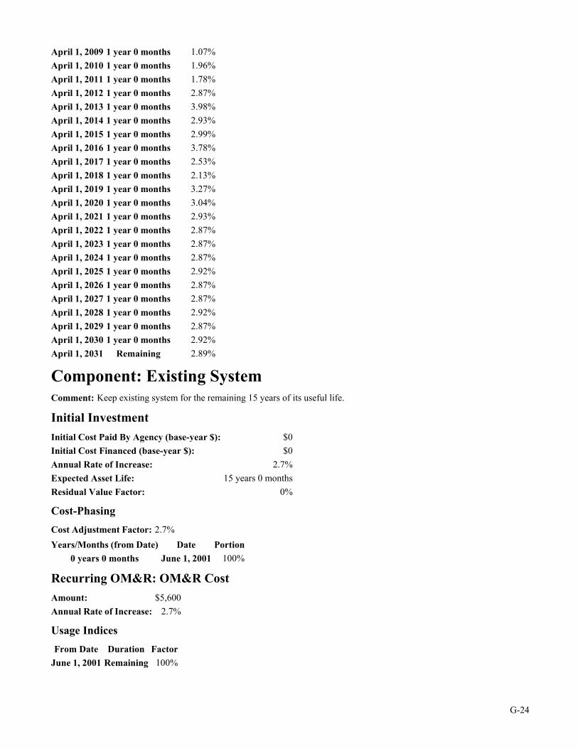
G-24

April 1, 2009 1 year 0 months 1.07% April 1, 2010 1 year 0 months 1.96% April 1, 2011 1 year 0 months 1.78% April 1, 2012 1 year 0 months 2.87% April 1, 2013 1 year 0 months 3.98% April 1, 2014 1 year 0 months 2.93% April 1, 2015 1 year 0 months 2.99% April 1, 2016 1 year 0 months 3.78% April 1, 2017 1 year 0 months 2.53% April 1, 2018 1 year 0 months 2.13% April 1, 2019 1 year 0 months 3.27% April 1, 2020 1 year 0 months 3.04% April 1, 2021 1 year 0 months 2.93% April 1, 2022 1 year 0 months 2.87% April 1, 2023 1 year 0 months 2.87% April 1, 2024 1 year 0 months 2.87% April 1, 2025 1 year 0 months 2.92% April 1, 2026 1 year 0 months 2.87% April 1, 2027 1 year 0 months 2.87% April 1, 2028 1 year 0 months 2.92% April 1, 2029 1 year 0 months 2.87% April 1, 2030 1 year 0 months 2.92% April 1, 2031 Remaining 2.89%

Component: Existing System Comment: Keep existing system for the remaining 15 years of its useful life.

Initial Investment Initial Cost Paid By Agency (base-year $): $0 Initial Cost Financed (base-year $): $0 Annual Rate of Increase: 2.7% Expected Asset Life: 15 years 0 months Residual Value Factor: 0%

Cost-Phasing Cost Adjustment Factor: 2.7% Years/Months (from Date) Date Portion

0 years 0 months June 1, 2001 100%

Recurring OM&R: OM&R Cost Amount: $5,600 Annual Rate of Increase: 2.7%

Usage Indices From Date Duration Factor

June 1, 2001 Remaining 100%

G-25

Alternative: Lighting Retrofit Recurring Contract: Annual Contract Payment Amount: $62,000 Annual Rate of Increase: 0%

Usage Indices From Date Duration Factor

June 1, 2001 10 years 0 months 100% June 1, 2011 Remaining 0%

Energy: Electricity Annual Consumption: 206,911.0 kWh Price per Unit: $0.04600 Demand Charge: $3,311 Utility Rebate: $0 Location: Arizona Rate Schedule: Commercial State: Arizona

Usage Indices From Date Duration Usage Index

June 1, 2001 Remaining 100%

Escalation Rates From Date Duration Escalation

April 1, 2001 1 year 0 months -0.6% April 1, 2002 1 year 0 months -0.34% April 1, 2003 1 year 0 months 1.51% April 1, 2004 1 year 0 months -1.38% April 1, 2005 1 year 0 months -0.65% April 1, 2006 1 year 0 months -2.21% April 1, 2007 1 year 0 months 0.04% April 1, 2008 1 year 0 months 1.64% April 1, 2009 1 year 0 months 1.07% April 1, 2010 1 year 0 months 1.96% April 1, 2011 1 year 0 months 1.78% April 1, 2012 1 year 0 months 2.87% April 1, 2013 1 year 0 months 3.98% April 1, 2014 1 year 0 months 2.93% April 1, 2015 1 year 0 months 2.99% April 1, 2016 1 year 0 months 3.78% April 1, 2017 1 year 0 months 2.53% April 1, 2018 1 year 0 months 2.13% April 1, 2019 1 year 0 months 3.27% April 1, 2020 1 year 0 months 3.04% April 1, 2021 1 year 0 months 2.93%

G-26

April 1, 2022 1 year 0 months 2.87% April 1, 2023 1 year 0 months 2.87% April 1, 2024 1 year 0 months 2.87% April 1, 2025 1 year 0 months 2.92% April 1, 2026 1 year 0 months 2.87% April 1, 2027 1 year 0 months 2.87% April 1, 2028 1 year 0 months 2.92% April 1, 2029 1 year 0 months 2.87% April 1, 2030 1 year 0 months 2.92% April 1, 2031 Remaining 2.89%

Component: New System Comment: Install new lighting/daylighting system financed through UC contract

Initial Investment Initial Cost Paid By Agency (base-year $): $0 Initial Cost Financed (base-year $): $390,480 Annual Rate of Increase: 2.7% Expected Asset Life: 20 years 0 months Residual Value Factor: 25%

Cost-Phasing Cost Adjustment Factor: 2.7% Years/Months (from Date) Date Portion

0 years 0 months June 1, 2001 100%

Recurring OM&R: Post-Contract OM Costs Amount: $3,000 Annual Rate of Increase: 2.7%

Usage Indices From Date Duration Factor

June 1, 2001 10 years 0 months 0% June 1, 2011 Remaining 100%

G-27

NIST BLCC 5.0-01: Comparative Analysis Consistent with Federal Life Cycle Cost Methodology and Procedures, 10 CFR, Part 436, Subpart A

Base Case: Existing Alternative: Lighting Retrofit

General Information File Name: C:\Program Files\BLCC5\projects\Class Exercise G3.xml Run Date: Thu Sep 20 14:33:10 EDT 2001 Project Name: Class Exercise G3 Project Location: Arizona Analysis Type: Federal Analysis, Financed Project Analyst: ASR Comment Replace existing lighting system with new system financed through a utility contract. Base Date of Study: June 1, 2001 Service Date: June 1, 2001 Study Period: 15 years 0 months(June 1, 2001 through May 31, 2016) Discount Rate: 6.1% Discounting Convention: End-of-Year

Comparison of Present-Value Costs PV Life-Cycle Cost Base Case Alternative Savings from Alternative

Initial Investment Costs Paid By Agency: Capital Requirements as of Base Date $0 $0 $0 Future Costs: Recurring and Non-Recurring Contract Costs $0 $454,492 -$454,492 Energy Consumption Costs $488,520 $93,365 $395,155 Energy Demand Charges $295,313 $32,479 $262,834 Energy Utility Rebates $0 $0 $0 Water Costs $0 $0 $0 Recurring and Non-Recurring OM&R Costs $65,432 $9,847 $55,585 Capital Replacements $0 $0 $0 Residual Value at End of Study Period $0 -$59,988 $59,988

------------ ------------ ------------ Subtotal (for Future Cost Items) $849,264 $530,195 $319,070

------------ ------------ ------------ Total PV Life-Cycle Cost $849,264 $530,195 $319,070

G-28

Net Savings from Alternative Compared with Base Case PV of Operational Savings $713,574 - PV of Differential Costs $394,504

------------ Net Savings $319,070

NOTE: Meaningful SIR, AIRR and Payback can not be computed for Financed Projects.

Comparison of Contract Payments and Savings from Alternative (undiscounted) Savings in Savings in Savings in Savings in Year Beginning Contract Costs Energy Costs Total Operational Costs Total Costs Jun 2001 -$62,000 $66,707 $72,457 $10,457 Jun 2002 -$62,000 $66,682 $72,588 $10,588 Jun 2003 -$62,000 $67,374 $73,439 $11,439 Jun 2004 -$62,000 $66,526 $72,755 $10,755 Jun 2005 -$62,000 $65,923 $72,320 $10,320 Jun 2006 -$62,000 $64,710 $71,280 $9,280 Jun 2007 -$62,000 $64,906 $71,653 $9,653 Jun 2008 -$62,000 $65,909 $72,839 $10,839 Jun 2009 -$62,000 $66,709 $73,825 $11,825 Jun 2010 -$62,000 $67,993 $75,302 $13,302 Jun 2011 $0 $69,327 $72,812 $72,812 Jun 2012 $0 $71,443 $75,022 $75,022 Jun 2013 $0 $74,159 $77,834 $77,834 Jun 2014 $0 $76,336 $80,111 $80,111 Jun 2015 $0 $78,712 $82,589 $228,159

Energy Savings Summary Energy Savings Summary (in stated units) Energy -----Average Annual Consumption----- Life-Cycle Type Base Case Alternative Savings Savings Electricity 1,082,633.0 kWh 206,911.0 kWh 875,722.0 kWh 13,134,031.8 kWh

Energy Savings Summary (in MBtu) Energy -----Average Annual Consumption----- Life-Cycle Type Base Case Alternative Savings Savings Electricity 3,694.1 MBtu 706.0 MBtu 2,988.1 MBtu 44,815.2 MBtu

G-29

Emissions Reduction Summary Energy -----Average Annual Emissions----- Life-Cycle Type Base Case Alternative Reduction Reduction Electricity

CO2 881,777.18 kg 168,523.77 kg 713,253.41 kg 10,697,336.55 kg SO2 1,080.53 kg 206.51 kg 874.02 kg 13,108.51 kg NOx 2,880.63 kg 550.54 kg 2,330.09 kg 34,946.56 kg

Total: CO2 881,777.18 kg 168,523.77 kg 713,253.41 kg 10,697,336.55 kg SO2 1,080.53 kg 206.51 kg 874.02 kg 13,108.51 kg NOx 2,880.63 kg 550.54 kg 2,330.09 kg 34,946.56 kg

G-30

Solution to Class Exercise G4

****************************************************************************** * N I S T B L C C: I N P U T D A T A L I S T I N G (ver. 4.9-01 ) * ****************************************************************************** FILE NAME: G4-1 FILE LAST MODIFIED ON 09-20-2001/14:35:22 PROJECT NAME: Class Exercise G4 PROJECT ALTERNATIVE: buy COMMENT: (NONE) GENERAL DATA: ------------- ANALYSIS TYPE: Federal Analysis--Projects Subject to OMB A-94 BASE DATE FOR LCC ANALYSIS: JUN 2001 STUDY PERIOD: 20 YEARS, 0 MONTHS SERVICE DATE: JUN 2001 DISCOUNT AND INTEREST RATES ARE Real (exclusive of general inflation) DISCOUNT RATE: 3.2% End-of-year discounting convention Escalation rates do not include general inflation CAPITAL ASSET COST DATA: ------------------------ INITIAL COST (BASE YEAR $) 5000000 EXPECTED ASSET LIFE (YRS/MTHS) 50/0 RESALE VALUE FACTOR 50.00% AVG PRICE ESC RATE(SERVICE PD.) 0.00% NUMBER OF REPLACEMENTS 0 NO REPLACEMENTS OPERATING, MAINTENANCE, AND REPAIR COST DATA: --------------------------------------------- ANNUAL RECUR OM&R COST ($): 200000 ESCALATION RATE FOR OM&R: 0.00% No non-annually-recurring OM&R costs reported. ENERGY-RELATED DATA: ----------------- NUMBER OF ENERGY TYPES = 0

G-31

****************************************************************************** * N I S T B L C C: I N P U T D A T A L I S T I N G (ver. 4.9-01 ) * ****************************************************************************** FILE NAME: G4-2 FILE LAST MODIFIED ON 09-20-2001/14:35:38 PROJECT NAME: Class Exercise G4 PROJECT ALTERNATIVE: lease COMMENT: (NONE) GENERAL DATA: ------------- ANALYSIS TYPE: Federal Analysis--Projects Subject to OMB A-94 BASE DATE FOR LCC ANALYSIS: JUN 2001 STUDY PERIOD: 20 YEARS, 0 MONTHS SERVICE DATE: JUN 2001 DISCOUNT AND INTEREST RATES ARE Real (exclusive of general inflation) DISCOUNT RATE: 3.2% End-of-year discounting convention Escalation rates do not include general inflation CAPITAL ASSET COST DATA: ------------------------ INITIAL COST (BASE YEAR $) 0 EXPECTED ASSET LIFE (YRS/MTHS) 50/0 RESALE VALUE FACTOR 0.00% AVG PRICE ESC RATE(SERVICE PD.) 0.00% NUMBER OF REPLACEMENTS 0 NO REPLACEMENTS OPERATING, MAINTENANCE, AND REPAIR COST DATA: --------------------------------------------- ANNUAL RECUR OM&R COST ($): 500000 ESCALATION RATE FOR OM&R: 0.00% No non-annually-recurring OM&R costs reported. ENERGY-RELATED DATA: ----------------- NUMBER OF ENERGY TYPES = 0

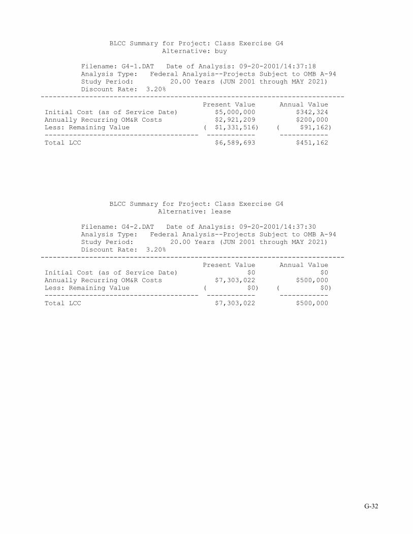
G-32

BLCC Summary for Project: Class Exercise G4 Alternative: buy Filename: G4-1.DAT Date of Analysis: 09-20-2001/14:37:18 Analysis Type: Federal Analysis--Projects Subject to OMB A-94 Study Period: 20.00 Years (JUN 2001 through MAY 2021) Discount Rate: 3.20% --------------------------------------------------------------------------- Present Value Annual Value Initial Cost (as of Service Date) $5,000,000 $342,324 Annually Recurring OM&R Costs $2,921,209 $200,000 Less: Remaining Value ( $1,331,516) ( $91,162) -------------------------------------- ------------ ------------ Total LCC $6,589,693 $451,162 BLCC Summary for Project: Class Exercise G4 Alternative: lease Filename: G4-2.DAT Date of Analysis: 09-20-2001/14:37:30 Analysis Type: Federal Analysis--Projects Subject to OMB A-94 Study Period: 20.00 Years (JUN 2001 through MAY 2021) Discount Rate: 3.20% --------------------------------------------------------------------------- Present Value Annual Value Initial Cost (as of Service Date) $0 $0 Annually Recurring OM&R Costs $7,303,022 $500,000 Less: Remaining Value ( $0) ( $0) -------------------------------------- ------------ ------------ Total LCC $7,303,022 $500,000

EM-1

Appropriate LCC Economic Measures (Evaluation Criterion)

NSType of Decision

LCC

Level of Efficiency

System Selection

Combination of Interdependent Systems

DISCOUNTED PBAIRRSIR

Economic Measures of Evaluation and Their Uses

no

yes (>1.0)

no

yes (descending order)**

yes (>0)

yes (maximum)

Project Priority (Independent Projects)

yes (minimum)Accept/Reject

yes (descending order)**

conditional* (< or = study period)

no

no

no

no

no

no

no

yes (>discount rate)

* Discounted Payback measure is consistent with LCC only if (1) cumulative net savings after payback is reached do not turn negative, and (2) residual values, if any, are included if payback is > or = study period.

** Fund in descending order of SIR or AIRR until budget is exhausted. Group of projects that fits within budget and has greatest overall net savings is best.

yes (minimum)

yes (minimum)

yes (maximum)

yes (maximum combined

NS)

yes (minimum combined

LCC)

no

no

no

AC-1

Acronyms AIRR

Adjusted Internal Rate of Return BOA

Basic Ordering Agreement Btu

British Thermal Units DoD

Department of Defense DOE

Department of Energy DPB

Discounted Payback ECM

Energy Conservation Measure ESCO

Energy Services Company ESPC

Energy Savings Performance Contract FEMP

Federal Energy Management Programs HVAC

Heating, Ventilation, and Air Conditioning GJ

Gigajoule (109 joules) kWh

Kilowatt Hours LCC

Life-Cycle Costs or Life-Cycle Costing MBtu

MBtu (106 x Btu) NS

Net Savings OM&R

Operation, Maintenance, and (Routine) Repairs OMB

Office of Management and Budget PB

Payback P/C/I

Planning/Contructions or Installation Period SIR

Savings-to-Investment Ratio SPB

Simple Payback

AC-2

SPV Single Present Value (Factor)

TLCC Total Life-Cycle Costs

UC or UESC Utility Contract or Utility Energy Services Contract

UPV Uniform Present Value (Factor)

UPV* Modified Uniform Present Value (Factor)

GL-1

Glossary Adjusted Internal Rate of Return (AIRR)

Annual yield from a project over the Study Period, taking into account investment of interim amounts.

Alternative Building System An installation or modification of an installation in a building intended primarily to reduce energy or water consumption or allow the use of renewable energy sources, or a primarily energy- or water-saving building system, including a renewable energy system, for consideration as part of the design for a new federal building.

Amount Financed Includes Implementation Costs and usually Financing Procurement Costs to comprise the amount borrowed by the Government agency to implement energy conservation measures.

Annually Recurring Costs Those costs incurred each year in an equal, constant dollar amount throughout the Study Period, or that change from year to year at a known rate.

Annual Value (Annual Worth) The time-equivalent value of past, present, or future cash flows expressed as an Annually Recurring Uniform amount over the Study Period.

Annual Value (Annual Worth or Uniform Capital Recovery) Factor A discount factor by which a present dollar amount may be multiplied to find its equivalent Annual Value, based on a given Discount Rate and a given period of time.

Base Case The situation against which an Alternative Building System is compared.

Base Date The beginning of the first year of the Study Period, generally the date on which the Life-Cycle Cost analysis is conducted.

Base Year The first year of the Study Period, generally the year in which the Life-Cycle Cost analysis is conducted.

Base-Year Energy Costs The quantity of energy delivered to the boundary of a Federal Building in the Base Year, multiplied by the Base-Year Price of fuel.

Base-Year Price The price of a good or service as of the Base Date.

Cash Flow The stream of costs and benefits (expressed for the purpose of this requirement in Constant Dollars) resulting from a project investment.

Compound Interest Factors or Formulas See Discount Factors or Formulas.

Constant Dollars Dollars of uniform purchasing power tied to a reference year (usually the Base Year) and exclusive of general price inflation or deflation.

Contract Payments An agreed-upon payment made annually or non-annually by the agency to repay the loan provided by an ESCO or UC for implementing energy savings measures.

GL-2

Contract Period or Contract Term The time period proposed by the contractor for repaying the loan provided to a Government agency to implement energy savings measures. It begins at the contract award date and includes the Installation Period and the Energy Savings Performance Period.

Cost Adjustment Factor The average annual rate at which the phased-in cost of a capital component is adjusted to its value in any year of the Planning/Construction/Installation Period. The Cost Adjustment Factor can, for example, be a contractual rate (sometimes equal to zero) or a rate determined by the agency.

Cost Effective The condition whereby an Alternative Building System saves more than it costs over the Study Period, where all Cash Flows are assessed in Constant Dollars and discounted to reflect the Time Value of Money.

Current Dollars Dollars of nonuniform purchasing power, including general price inflation or deflation, in which actual prices are stated. (With zero inflation or deflation, current dollars are identical to constant dollars.)

Debt Service The sum of interest payments and principal payments which comprise or are part of the Contract Payment to an ESCO or UC.

Demand Charge That portion of the charge for electric service based on the plant and equipment costs associated with supplying the electricity consumed.

Differential Cost The difference in the costs of an Alternative Building System and the Base Case.

Differential Energy Price Escalation Rate The difference between a projected general rate of Inflation and the projected rate of price increase assumed for energy.

Discount Factors Multiplicative numbers used to convert Cash Flows occurring at different times to their equivalent amount at a common time. Discount factors are obtained by solving Discount Formulas based upon one dollar of value and an assumed Discount Rate and time.

Discount Formula An expression of a mathematical relationship which enables the conversion of dollars at a given point in time to their equivalent amount at some other point in time.

Discount Rate The rate of interest, reflecting the investor's Time Value of Money (or opportunity cost), that is used in Discount Formulas or to select Discount Factors which in turn are used to convert ("discount") Cash Flows to a common time. Real Discount Rates reflect Time Value of Money apart from changes in the purchasing power of the dollar and are used to discount Constant Dollar Cash Flows; Nominal Discount Rates include changes in the purchasing power of the dollar and are used to discount Current Dollar Cash Flows.

Discounted Payback Period The time required for the cumulative savings from an investment to pay back the Investment Costs and other accrued costs, taking into account the Time Value of Money.

GL-3

Discounting A technique for converting Cash Flows occurring over time to time-equivalent values, at a common point in time, adjusting for the Time Value of Money.

Disposal Cost See Residual Value.

Economic Life That period of time over which a Building or Building System is considered to be the lowest-cost alternative for satisfying a particular need.

Energy Conservation Measure (ECM) Defined as the installation of new equipment/facilities, modification, or alteration of existing government equipment/facilities, or revised operations and maintenance procedures to reduce energy consumption of facilities/energy systems.

Energy Cost The annual cost of fuel or energy used to operate a building or building system, as billed by the utility or supplier (including Demand Charges, if any). Energy Costs are incurred during the Service Period only. Energy consumed in the construction or installation of a new building or building system is not included in this cost.

Energy Savings Performance Contracts Contracts authorized by the Energy Policy Act of 1992 (EPACT), which offer alternative financing of energy and water efficiency improvements in federal buildings and allow the Federal Government to retain a portion of the energy savings and all equipment installed.

Energy Savings Performance Period (ESPC) The period (typically in years) from the date an ECM is operational and accepted by the Government agency to the end of the Contract Period. The Energy Savings Performance Period may also be referred to as the "service period."

Federal Government The U.S. Government.

Financing Procurement Costs May be added to Implementation Costs to comprise the total amount financed by an ESCO or UC.

Future Value The time-equivalent value of past, present, or future Cash Flows expressed as of some future point in time.

Implementation Costs May include survey costs, feasibility study costs, design expenses, and construction costs, which may be paid by an agency or included in the Contract Payment proposed by ESCO or UC.

Initial Investment Costs The initial costs of design, engineering, purchase, and installation, exclusive of "Sunk Costs," all of which are assumed to occur as a lump sum at the beginning of the Base Year or during the Planning/Construction/Installation Period for purposes of making the life-cycle cost analysis.

Inflation A rise in the general price level, or, put another way, a decline in the general purchasing power of the dollar.

GL-4

Installation Period The period from the date of contract award to the date all contracted energy conservation measures are operational and accepted by the agency. Installation period may also be referred to as "construction period."

Internal Rate of Return Annual yield from a project over the Study Period, i.e., the compound rate of interest which, when used to discount Cash Flows of an Alternative Building System, will result in zero Net Savings (Net Benefits).

Life-Cycle Cost (LCC) The total discounted dollar costs of owning, operating, maintaining, and disposing of a building or building system over the Study Period (see Life-Cycle Cost Analysis).

Life-Cycle Cost Analysis (LCCA) A method of economic evaluation that sums discounted dollar costs of initial investment (less Resale, Retention, or Salvage Value), replacements, operations (including energy and water usage), and maintenance and repair of a building or building system over the Study Period (see Life-Cycle Cost). Also, as used in this program, LCCA is a general approach to economic evaluation encompassing several related economic evaluation measures, including Life-Cycle Cost (LCC), Net Benefits (NB) or Net Savings (NS), Savings-to-Investment Ratio (SIR), and Adjusted Internal Rate of Return (AIRR), all of which take into account long-term dollar impacts of a project.

Liquid Petroleum Gas (LPG) Propane, butane, ethane, pentane, or natural gasoline.

Market Interest Rate The nominal loan interest rate (including inflation) applied by the ESCO or UC to the Amount Financed to compute annual Contract Payments.

Measures of Economic Evaluation The various ways in which project cash flows can be combined and presented to describe a measure of project cost effectiveness. The measures used to evaluate FEMP projects are Life-Cycle Cost (LCC), Net Savings (NS), Savings-to-Investment Ratio (SIR), Adjusted Internal Rate of Return (AIRR). Discounted Payback (DPB) and Simple Payback (SPB) are measures of evaluation not fully consistent with the LCC method but are used as supplementary measures in some federal programs.

Modified Uniform Present Value (Worth) (UPV* or UPW*) Factor A discount factor used to convert an annual amount escalating at a constant rate to a time-equivalent Present Value. The FEMP UPV* Factor indicates a discount factor from a special set published by the U.S. Department of Energy, Federal Energy Management Program, for computing present value energy costs based on variable energy price projections.

Mutually Exclusive Projects Projects where the acceptance of one precludes acceptance of the others. Examples are whether to use single-glazing, double-glazing or triple-glazing for a window; or R11, R19, or R30 levels of insulation in an attic.

Net Savings (Net Benefits) Time-adjusted savings (or benefits) less time-adjusted differential costs taken over the Study Period for an Alternative Building System relative to the base case.

Nominal Discount Rate The rate of interest (market interest rate) reflecting the time value of money stemming from both inflation and the real earning power of money over time.

GL-5

Nonmutually Exclusive Projects Projects where the acceptance of one alternative does not preclude the acceptance of the others. Examples are wall insulation and ceiling insulation.

Nonrecurring Costs Costs that are not uniformly incurred annually over the Study Period.

Nonfuel Operation, Maintenance, and Repair (OM&R) Costs Labor and material costs required for routine upkeep, repair, and operation, exclusive of energy costs.

Nonmutually Exclusive Projects Projects where the acceptance of one does not preclude the acceptance of the others. Examples are wall insulation and ceiling insulation. (For contrast, see Mutually Exclusive.)

Performance Period Expenses May include management/administration costs, operation and maintenance costs, repair and replacement costs, measurement and verification costs, permits and licenses costs, insurance costs, property taxes, and other costs (e.g., "margin"), which may be paid by agency or included in the Contract Payment proposed by ESCO or UC.

Planning/Construction Period The period beginning with the Base Date and continuing up to the Service Date, during which only Initial Investment Costs are incurred.

Post-Contract Period The period between the end of the Contract Period (Contract Term) and the end of the Study Period.

Present Value (Present Worth) The time-equivalent value of past, present or future Cash Flows as of the beginning of the Base Year.

Present Value (Present Worth) Factor A discount factor by which a future dollar amount may be multiplied to find its equivalent Present Value as of the Base Date. Single Present Value Factorsare used to convert single future amounts to Present Values. Uniform Present Value Factors and Modified Present Value Factors are used to convert Annually Recurring amounts to Present Values.

Real Discount Rate The rate of interest reflecting the portion of the time value of money attributable to the real earning power of money over time and not to general price inflation.

Renewable Energy Energy obtained from sources that are essentially inexhaustible (unlike, for instance, fossil fuels of which there is a limited supply). Renewable sources of energy include wind energy, geothermal energy, hydroelectric energy, photovoltaic and solar energy, biomass, and waste.

Replacement Costs Future costs included in the capital budget to replace a building system during the Study Period.

Resale Value See Residual Value.

Residual Value The estimated value, net of any Disposal Costs, of any building or building system removed or replaced during the Study Period; or remaining at the end of the Study Period; or recovered through resale or reuse at the end of the Study Period (also called Resale Value or Salvage Value, or Retention Value).

GL-6

Retention Value See Residual Value.

Retrofit The installation of an Alternative Building System in an Existing Federal Building.

Risk Attitude The willingness of decision makers to take chances or to gamble on investments of uncertain outcome. Risk attitudes are generally classified as risk-averse, risk-neutral, or risk-taking.

Risk Exposure The probability of investing in a project whose economic outcome is less favorable than what is economically acceptable.

Salvage Value See Residual Value.

Savings-to-Investment Ratio (SIR) A ratio computed from a numerator of discounted energy and/or water savings, plus (less) savings (increases) in Nonfuel Operation and Maintenance Costs, and a denominator of increased Investment Costs plus (less) increased (decreased) Replacement Costs, net of Residual Value (all in present-value terms), for an Alternative Building System as compared with a Base Case.

Sensitivity Analysis Testing the outcome of an evaluation to changes in the values of one or more system parameters from the initially assumed values.

Service Date The point in time during the Study Period when a building or building system is put into use, and operating, maintenance, and repair costs (including energy and water costs) begin to be incurred.

Service Period The period of time starting with the Service Date and continuing through the end of the Study Period.

Simple Payback Period (SPB) A measure of the length of time required for cumulative savings from a project to recover the Investment Cost and other accrued costs, without taking into account the Time Value of Money.

Single Present Value (Worth) (SPV or SPW) Factor The discount factor used to convert single future benefit and cost amounts to Present Value.

Study Period The length of the time period covered by the economic evaluation. This includes both the Planning/Construction Period and the Service Period.

Sunk Costs Costs which have been incurred or committed to prior to the Life-Cycle Cost analysis and which, therefore, should not be considered in making a current project decision since the costs cannot be changed.

Time-of-Use Rate The charge for service during periods of the day based on the cost of supplying the service at that particular time of the day.

Time Value of Money The time-dependent value of money. If project Cash Flows are stated in Constant Dollars, their adjustment to a common time basis is necessary to take into account the real earning potential of investments over time. If project cash flows are stated in Current Dollars, their

GL-7

adjustment to a common time basis is necessary to take into account not only the real earning potential over time, but also price inflation or deflation.

Uniform Present Value (Worth) (UPV or UPW) Factor The discount factor used to convert uniform annual values to a time-equivalent Present Value.

Useful Life The period of time over which a Building or Building System continues to generate benefits or savings.

Utility Contracts (UC) or Utility Energy Services Contracts (UESC) Contracts (Area-Wide Contracts or Basic Ordering Agreements) between a government agency and a utility company, which allow the Federal Government to implement energy and water conservation measures through financing provided by the utility.

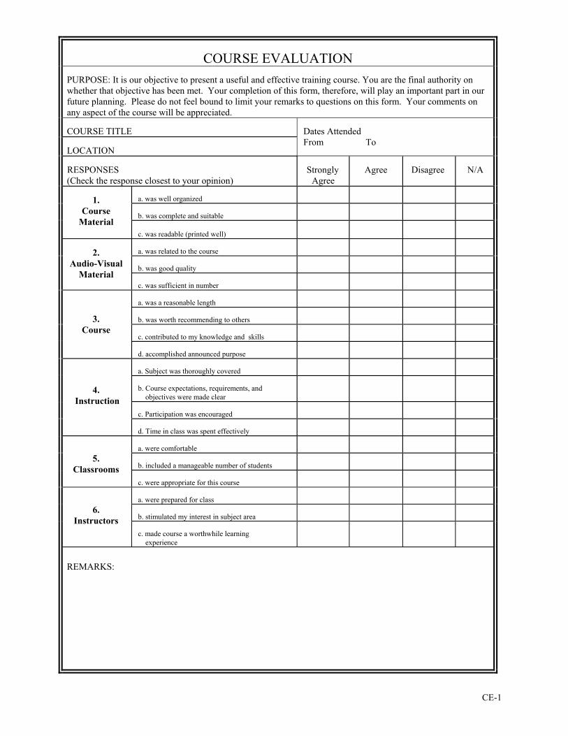
CE-1

COURSE EVALUATION

PURPOSE: It is our objective to present a useful and effective training course. You are the final authority on whether that objective has been met. Your completion of this form, therefore, will play an important part in our future planning. Please do not feel bound to limit your remarks to questions on this form. Your comments on any aspect of the course will be appreciated. COURSE TITLE LOCATION

Dates Attended From To

RESPONSES (Check the response closest to your opinion)

Strongly Agree

Agree

Disagree

N/A

a. was well organized

b. was complete and suitable

1.

Course Material

c. was readable (printed well)

a. was related to the course

b. was good quality

2.

Audio-Visual Material

c. was sufficient in number

a. was a reasonable length

b. was worth recommending to others

c. contributed to my knowledge and skills

3. Course

d. accomplished announced purpose

a. Subject was thoroughly covered

b. Course expectations, requirements, and objectives were made clear

c. Participation was encouraged

4. Instruction

d. Time in class was spent effectively

a. were comfortable

b. included a manageable number of students

5. Classrooms

c. were appropriate for this course

a. were prepared for class

b. stimulated my interest in subject area

6. Instructors

c. made course a worthwhile learning experience

REMARKS:

CE-2

COURSE EVALUATION (Continued) 7. OVERALL INSTRUCTOR EVALUATION (Check your opinion)

a. Knowledge of the subject Excellent Good Fair Poor b. Ability to teach Excellent Good Fair Poor

8. WOULD YOU ADD OR EMPHASIZE ANY SUBJECT MATTER AREAS IN SUBSEQUENT COURSE SESSIONS?

yes no If "yes," list these areas and give your reasons: 9. WOULD YOU DELETE OR DE-EMPHASIZE ANY SUBJECT-MATTER AREAS?

yes no If "yes," list these areas and give your reasons: 10. AS A RESULT OF YOUR PARTICIPATION IN THIS COURSE, WHAT ADDITIONAL RELATED TRAINING SHOULD BE MADE AVAILABLE? 11. OTHER COMMENTS. PLEASE MAKE ANY COMMENTS RELATIVE TO THIS COURSE, EITHER GENERAL OR SPECIFIC. SIGNATURE AND TITLE (optional)

ORGANIZATION

DATE