1

Progressive Expenditure Taxes and Growth

William Scarth*McMaster University

May 2005

Abstract

Standard tax-policy advice suggests cutting income taxes, and relying more onexpenditure taxes, to raise growth. The standard basis for this advice is endogenousgrowth theory, and the proof that an expenditure tax is preferred has involved acomparison of two proportional taxes in models with just one group of households. Thereis no formal evaluation of the concern that a proportional expenditure tax is regressive.Policy analysts have simply presumed that there would be support for a progressiveexpenditure tax, over a progressive income tax, if this option were formally modeled.This paper examines this presumption. Following Mankiw (2000), our simpleendogenous growth model involves two groups. The first is an infinitely lived familydynasty that smooths consumption in the usual fashion. The second group is impatientand does not accumulate physical capital. Beyond the investment in human capital that isrequired to keep a job, these individuals simply consume their income (labour earningsplus a transfer payment). The transfer is financed by taxes levied on the other (richer)group. We find that both groups prefer that the transfer be financed by an income tax, notan expenditure tax. The intuition follows from the fact that redistribution creates asecond-best initial condition, that is similar to that concerning government spending oninfrastructure (discussed in Barro and Sala-i-Martin (1995)). They show that lowergrowth is preferred if government spending is fixed at a non-optimal proportion of thegrowing GDP, since growth accentuates this distortion. There is a similar distortion here.From the selfish point of view of the rich, any positive transfer is non-optimal, andgrowth magnifies this problem. Since the analysis does not support conventional wisdom,it challenges policy analysts to identify the analytical underpinnings of their views.

*Without implication, I thank Jon Kesselman, Lonnie Magee and Krishna Sengupta forhelpful comments.

2

1. Introduction

Many economists have called for a shift in tax policy: a decreased reliance on incometaxation and an increased reliance on expenditure taxes (see, for example, Mintz (2001),Kesselman (2004) and the numerous references contained in these studies). The standardanalytical underpinning for this tax-reform proposal is endogenous growth theory. Whileless emphasis is given to equity considerations (since standard growth theory involves asingle representative agent), policy analysts sometimes call for a progressive expendituretax – to avoid the regressivity that would otherwise accompany the use of sales taxes.

The purpose of this paper is to use a simple version of endogenous growth theory toreview this debate. Two results emerge from this review. First, considering proportionaltaxes, if the optimal tax question is decided in a second-best setting in which governmentis “too big,” the analysis does not support elimination of the income tax. Many policyanalysts argue both that government is “too big” and that income taxes are “bad.” Thepaper challenges these analysts to identify the analytical underpinnings of their views.The second result follows from an extension that involves two groups of households (asadvocated by Mankiw (2000)). The first group pursues the standard consumption-smoothing strategy (as in Ramsey (1928)), so for this segment of the population, there isno difference from the earlier analysis. But the second group is more impatient. Theseindividuals have a sufficiently high rate of time preference that they do not accumulatephysical capital. They live “hand-to-mouth,” consuming all the income they receive inevery period (beyond what is necessary to maintain the human capital that is required tobe employed). This version of the model permits an analysis of a progressive expendituretax; it does not provide clear support at all for the proposition that a progressiveexpenditure tax dominates a progressive income tax.

The remainder of the paper is organized as follows. In section 2, we explain the basicmodel and methodology, and we assess the relative appeal of proportional income taxesand expenditure taxes in a setting with no hand-to-mouth individuals. In section 3, wedistinguish between physical and human capital, and we focus on hand-to-mouthhouseholds and progressive taxes. Concluding remarks are offered in section 4, and sometechnical derivations are reported in the Appendix.

2. Proportional Taxes

We begin with the proposition that total output produced each period, Y, is used in twoways. First, it is purchased by households to be consumed that period, C. Second, it ispurchased by households to add to their stock of capital, K. ∆K refers to that period’sincrease in capital. The supply-equals-demand statement is

.KCY ∆+= (1)

3

Next we specify the production process; in this initial case, it is very simple – output isproportional to the one input that is used in the production process, K:

.rKY = (2)

r – the rate of return on capital – is the amount that output increases as additional units ofthe input are hired (the average and marginal product of capital). r is the pre-tax returnthat households earn on their saving. There are two potentially controversial aspects ofthis specification of the nation’s input-output relationship. First, there is no diminishingreturns (as more capital is employed, its marginal product does not fall). The economy’sequilibrium growth rate is independent of fiscal policy if this assumption is not made, sowe follow that standard practice here. Second, once the output emerges from thisproduction process in the form of consumer goods, it is costless for society to convert thatnew output into additional capital. Again, this assumption is made to keep the paperconsistent with standard analysis. Also, for simplicity, we ignore depreciation of capital.

In this initial specification, the government has just one function; it levies a proportionalincome tax rate, t, on the income that households earn by employing their capital, and aproportional sales tax rate, s, on household consumption spending. The government usesthis revenue to finance transfer payments, R, to households. The government’s balanced-budget constraint is

.sCtrKR += (3)

This specification of government is rather contrived, since all households are identical.There seems little point in having the government impose taxes that can distort eachhousehold’s decisions, when the only use for that revenue is to transfer the funds back tothat same household. We make this assumption simply because it is standard in theliterature. Also, it serves as a base upon which we can build a more interesting analysis ofgovernment policy in later sections of the paper.

The only other relationship that is needed to complete this initial analysis is the one thatdescribes how households make their consumption-vs-saving decision. We assume thattheir objective is to maximize their utility, which is defined by the following function:

∑∞

=

+=0

].[ln)]1/(1[i

ii Cputility

This utility function involves three features. First, at any point in time (indexed by i)), theadditions to utility that accompany higher levels of consumption get smaller, the higher isthe level of consumption initially. The logarithmic relationship is the simplest functionthat can impose this standard assumption of diminishing marginal utility of consumption.The second feature of the utility function is that it imposes the fact that households areimpatient. Parameter p is the household’s rate of time preference; it is the discount ratethat is used to capture the idea that the utility of future consumption is lower than thatassociated with current consumption. The third feature of the utility function is that it

4

involves households forming a plan that extends infinitely into the future. To rationalizethis feature, it is useful to think of the household as an ongoing family dynasty.

Households are assumed to maximize utility subject to their budget constraint:

.sCtrKRrKKC −−+=∆+

This constraint states that households pay for their consumption and capital accumulation(saving) by spending all their after-tax income and their transfer payment. We outline theformal solution of this constrained maximization in the Appendix. Here we focus on anintuitive interpretation of what constitutes optimal behaviour. To stretch their limitedbudget as far as possible, households must arrange their purchases so that the additionalsatisfaction (the marginal utility, MU) that is had for each unit of income that needs to bepaid, is identical at each point in time. For example,

.)/()/( futurepresent priceMUpriceMU =

If this equality did not hold (say because the left-hand side exceeded the right-hand side),households could increase satisfaction by transferring spending from the future to thepresent. As they did so, the marginal utility of present consumption would fall and thatfor the future would rise. The payoff for further reallocation of spending would vanishwhen these changes in marginal utility just eliminated the original excess of the left-handexpression over that on the right.

To apply this general principle in the present setting, we pick the price of currentconsumption as the numeraire, and set this price equal to unity. Adopting this conventionmakes the price of future consumption equal to (1/(1+r(1-t)), since – by waiting for aperiod to consume – households can earn the after-tax rate of interest on each unit ofincome. Given the logarithmic utility function, the marginal utility of present (i = 0)consumption is )/1( 0C and the marginal utility of future (i = 1) consumption is

)).)1/((1( 1Cp+ Substituting these expressions into the optimum-consumption condition,

we have: ).1/())1(1(/ 01 ptrCC +−+= Subtracting unity from both sides, andsimplifying by approximating (1+p) by unity, we end with

ptrCC −−=∆ )1(/ (4)

The intuition behind this behavioural rule is straightforward. Households save as long asthe after-tax return on capital exceeds their rate of impatience, and this saving generatesthe income necessary to have a positive percentage growth rate for consumption.

We now write the four numbered equations in a more compact form. We focus on abalanced-growth equilibrium in which consumption, output, and the capital stock allgrow at the same rate: ,/// KKYYCCn ∆=∆=∆= and with the tax rates, t and s, theratio of consumption-to-capital, c = C/K, and the ratio of transfer payments-to-GDP, z =

5

R/Y, all constant. To accomplish this, we divide (1) and (3) through by K and Yrespectively, and use (2) and the balanced growth assumption to simplify the results:

ncr += (5)rsctz /+= (6)

ptrn −−= )1( (7)

Equations (5) through (7) solve for the economy’s growth rate, n, the consumption-to-capital ratio, c, and one of the tax rates (we assume that the sales tax rate, s, is residuallydetermined by the model). The equations indicate how these three variables are affectedby any change we wish to assume in the technology parameter, r, the taste parameter, p,and the government’s exogenous instruments – the transfers-to-GDP ratio, z, and theincome tax rate, t.

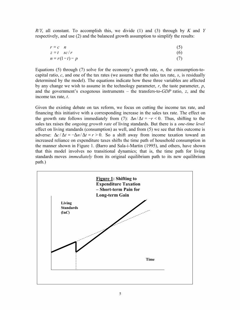
Given the existing debate on tax reform, we focus on cutting the income tax rate, andfinancing this initiative with a corresponding increase in the sales tax rate. The effect onthe growth rate follows immediately from (7): .0/ <−=∆∆ rtn Thus, shifting to thesales tax raises the ongoing growth rate of living standards. But there is a one-time leveleffect on living standards (consumption) as well, and from (5) we see that this outcome isadverse: .0// >=∆∆−=∆∆ rtntc So a shift away from income taxation toward anincreased reliance on expenditure taxes shifts the time path of household consumption inthe manner shown in Figure 1. (Barro and Sala-i-Martin (1995), and others, have shownthat this model involves no transitional dynamics; that is, the time path for livingstandards moves immediately from its original equilibrium path to its new equilibriumpath.)

LivingStandards(lnC)

Time

Figure 1: Shifting toExpenditure Taxation– Short-term Pain forLong-term Gain

6

Given that there is short-term pain to achieve long-term gain, it is not immediately clearthat this tax substitution is supported. But we can address this issue by using thehousehold utility function. It is shown in the Appendix that when the present-valuesummation is worked out, overall social welfare (SW) is

ppnCSW /)]/([ln 0 += (8)

where 00 cKC = and 0K is the initial capital stock, at the time when the tax substitutiontakes effect. From (8), we can determine the effect on overall welfare of the taxsubstitution:

ptnptcctSW /)]/)(/1()/)(/1[(/ ∆∆+∆∆=∆∆

Using the one-time-level and ongoing-growth-rate effects reported above, we have

)/()(/ 2cpcprtSW −=∆∆

which can be simplified by using (5) and (7):

.0)/()(/ 22 <−=∆∆ cptrtSW

The fact that this expression is negative indicates that the government can raise peoples’material welfare by cutting the income tax rate – all the way to zero. This is the standardproof that we should rely on expenditure, not income, taxes to finance the transferpayments. Because the generosity of the transfer does not affect the household’sconsumption-saving choice, there is no such thing as an “optimal” value for transfers.Whatever level is arbitrarily chosen has to be financed by expenditure taxes if thegovernment wishes to maximize the material welfare of its citizens.

We now consider a sensitivity test, by asking how the optimal-tax conclusion is affectedby our replacing the government transfer payment with a program whereby thegovernment buys a fraction of the GDP and distributes it free to users (as in the case ofgovernment-provided health care). We continue to assume that no resources are neededto convert newly produced consumer goods into new capital or (now) into thegovernment service. Thus, the economy’s production function remains (2), and thesupply-equals-demand relationship becomes

GKCY +∆+= (1a)

where G is the level of the government-provided good each period. The governmentbudget constraint becomes

.sCtrKG += (3a)

7

Finally, we assume that households value the government-provided good, so there aretwo term’s in each period’s utility function:

∑∞

=

++=0

].ln[ln)]1/(1[i

iii GfCputility

Parameter f indicates the relative value that households attach to the government service.Since the government imposes the level of government spending, individual householdsstill have only one choice to make; they must choose their accumulation of capital with aview to maximizing the present discounted value of private consumption. The solution tothat problem is still equation (4).

The model is now defined by equations (1a), (2), (3a) and (4). Defining g = G/Y as theratio of the government’s spending to GDP, these relationships can be re-expressed incompact form:

ncgr +=− )1( (5a)rsctg /+= (6a)

ptrn −−= )1( (7)

and the modified overall material welfare function is

ppnfGCSW /)]/)(1(ln[ln 00 +++= (8a)

It remains true that ,// rtntc =∆∆−=∆∆ but before we use these outcomes, we focus onthe question of the optimal level of government program spending. We use the sameprinciple that we applied to households above. In the present application (to thegovernment’s choice), that principle is to set government spending so that

.)/()/( goodprovidedgovernmentgoodnconsumptioprivate priceMUpriceMU =

Since the price of both goods is unity, this condition requires 1/C = f/G; that is, theoptimal program-spending-to-GDP ratio is g* = fc/r. This definition is used to simplifythe overall welfare effect of varying the income tax rate. The result is:

].*))][(/([/ 22 tggcprtSW −−=∆∆

As before, material welfare is maximized when this expression is zero, and this requiresno income tax (t = 0) only if government is set optimally (g = g*). If, however,government spending is “too big” (g > g*), there should be an income tax.

What is the intuition behind the result that income taxes should be used to finance someof the government when government is too big? The answer hinges on the fact that this

8

resource misallocation is in terms of a fixed proportion of a growing GDP. With growth,the magnitude of the distortion is being magnified. In this case, then, growth has a “bad”dimension. This is why it becomes “good” to rely, to some extent, on the anti-growthinstrument for raising tax revenue (the income tax rate). Barro and Sala-i-Martin (1995,pp 144-161) consider a very similar model. But their government-provided good is“infrastructure,” and it enters the production function instead of the utility function.Nevertheless, the same dependence of the optimal tax question on second-bestconsiderations – whether the government has set its expenditure “properly” – is stressed.

We conclude that we cannot know whether the actual economy involves the “preferred”ratio of income to sales tax rates or not, unless we know whether the government is “toobig” or not, and by how much. Many pro-growth policy analysts defend two propositions:(i) that income taxes are too high relative to sales taxes, and (ii) that the governmentsector is too big. Our analysis has shown that the more correct these analysts areconcerning the second proposition, the less standard growth theory supports their firstproposition. One purpose of this paper is to identify this tension that policy analysts donot appear to be aware of.

3. Progressive Taxes

Thus far, there has been just one input in the production process, and we have interpretedthat input quite broadly – as including both physical and human capital. For theremainder of the paper, we wish to contrast patient households who plan inter-temporallyand acquire physical capital (as discussed above) with households that always spend theirentire labour income and transfer payments. To make this comparison explicit, we mustnow distinguish physical capital (K) from human capital (H). The supply-equals-demandequation becomes

GHKCY +∆+∆+=

since output is either consumed privately, consumed in the form of a government-provided good, or used to accumulate physical and human capital.

Both forms of capital, the government service, and consumer goods, are produced via thefollowing production function:

bb HaKY −= 1

with b a positive fraction. By defining B = H/K and ,1 baBA −= the production functioncan be re-expressed as Y = AK – the same form as that used in Section 2 above. Barro andSala-i-Martin (1995, pp 144-146) suggest this interpretation for the standard AKproduction function.

Compared to the tax-policy literature, this specification of the production functioninvolves a “middle-of-the-road” assumption concerning the factor intensities that are

9

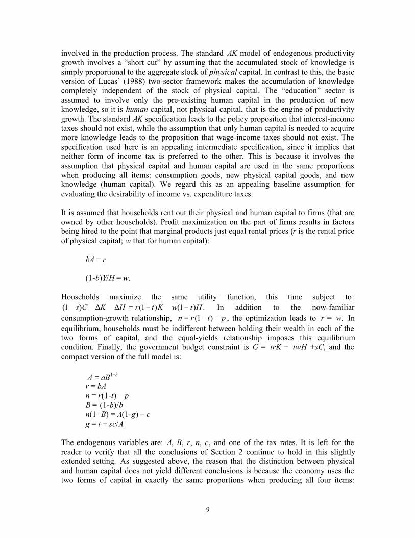
involved in the production process. The standard AK model of endogenous productivitygrowth involves a “short cut” by assuming that the accumulated stock of knowledge issimply proportional to the aggregate stock of physical capital. In contrast to this, the basicversion of Lucas’ (1988) two-sector framework makes the accumulation of knowledgecompletely independent of the stock of physical capital. The “education” sector isassumed to involve only the pre-existing human capital in the production of newknowledge, so it is human capital, not physical capital, that is the engine of productivitygrowth. The standard AK specification leads to the policy proposition that interest-incometaxes should not exist, while the assumption that only human capital is needed to acquiremore knowledge leads to the proposition that wage-income taxes should not exist. Thespecification used here is an appealing intermediate specification, since it implies thatneither form of income tax is preferred to the other. This is because it involves theassumption that physical capital and human capital are used in the same proportionswhen producing all items: consumption goods, new physical capital goods, and newknowledge (human capital). We regard this as an appealing baseline assumption forevaluating the desirability of income vs. expenditure taxes.

It is assumed that households rent out their physical and human capital to firms (that areowned by other households). Profit maximization on the part of firms results in factorsbeing hired to the point that marginal products just equal rental prices (r is the rental priceof physical capital; w that for human capital):

bA = r

(1-b)Y/H = w.

Households maximize the same utility function, this time subject to:.)1()1()1( HtwKtrHKCs −+−=∆+∆++ In addition to the now-familiar

consumption-growth relationship, ptrn −−= )1( , the optimization leads to r = w. Inequilibrium, households must be indifferent between holding their wealth in each of thetwo forms of capital, and the equal-yields relationship imposes this equilibriumcondition. Finally, the government budget constraint is G = trK + twH +sC, and thecompact version of the full model is:

baBA −= 1

r = bAn = r(1-t) – pB = (1-b)/bn(1+B) = A(1-g) – cg = t + sc/A.

The endogenous variables are: A, B, r, n, c, and one of the tax rates. It is left for thereader to verify that all the conclusions of Section 2 continue to hold in this slightlyextended setting. As suggested above, the reason that the distinction between physicaland human capital does not yield different conclusions is because the economy uses thetwo forms of capital in exactly the same proportions when producing all four items:

10

consumer goods, the government good, new physical capital goods, and new knowledge(human capital).

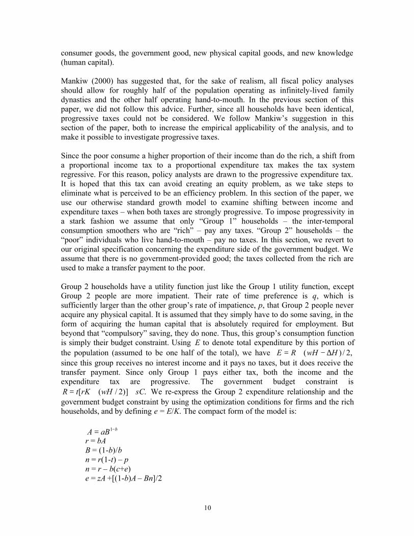
Mankiw (2000) has suggested that, for the sake of realism, all fiscal policy analysesshould allow for roughly half of the population operating as infinitely-lived familydynasties and the other half operating hand-to-mouth. In the previous section of thispaper, we did not follow this advice. Further, since all households have been identical,progressive taxes could not be considered. We follow Mankiw’s suggestion in thissection of the paper, both to increase the empirical applicability of the analysis, and tomake it possible to investigate progressive taxes.

Since the poor consume a higher proportion of their income than do the rich, a shift froma proportional income tax to a proportional expenditure tax makes the tax systemregressive. For this reason, policy analysts are drawn to the progressive expenditure tax.It is hoped that this tax can avoid creating an equity problem, as we take steps toeliminate what is perceived to be an efficiency problem. In this section of the paper, weuse our otherwise standard growth model to examine shifting between income andexpenditure taxes – when both taxes are strongly progressive. To impose progressivity ina stark fashion we assume that only “Group 1” households – the inter-temporalconsumption smoothers who are “rich” – pay any taxes. “Group 2” households – the“poor” individuals who live hand-to-mouth – pay no taxes. In this section, we revert toour original specification concerning the expenditure side of the government budget. Weassume that there is no government-provided good; the taxes collected from the rich areused to make a transfer payment to the poor.

Group 2 households have a utility function just like the Group 1 utility function, exceptGroup 2 people are more impatient. Their rate of time preference is q, which issufficiently larger than the other group’s rate of impatience, p, that Group 2 people neveracquire any physical capital. It is assumed that they simply have to do some saving, in theform of acquiring the human capital that is absolutely required for employment. Butbeyond that “compulsory” saving, they do none. Thus, this group’s consumption functionis simply their budget constraint. Using E to denote total expenditure by this portion ofthe population (assumed to be one half of the total), we have ,2/)( HwHRE ∆−+=since this group receives no interest income and it pays no taxes, but it does receive thetransfer payment. Since only Group 1 pays either tax, both the income and theexpenditure tax are progressive. The government budget constraint is

.)]2/([ sCwHrKtR ++= We re-express the Group 2 expenditure relationship and thegovernment budget constraint by using the optimization conditions for firms and the richhouseholds, and by defining e = E/K. The compact form of the model is:

baBA −= 1

r = bAB = (1-b)/bn = r(1-t) – pn = r – b(c+e)e = zA +[(1-b)A – Bn]/2

11

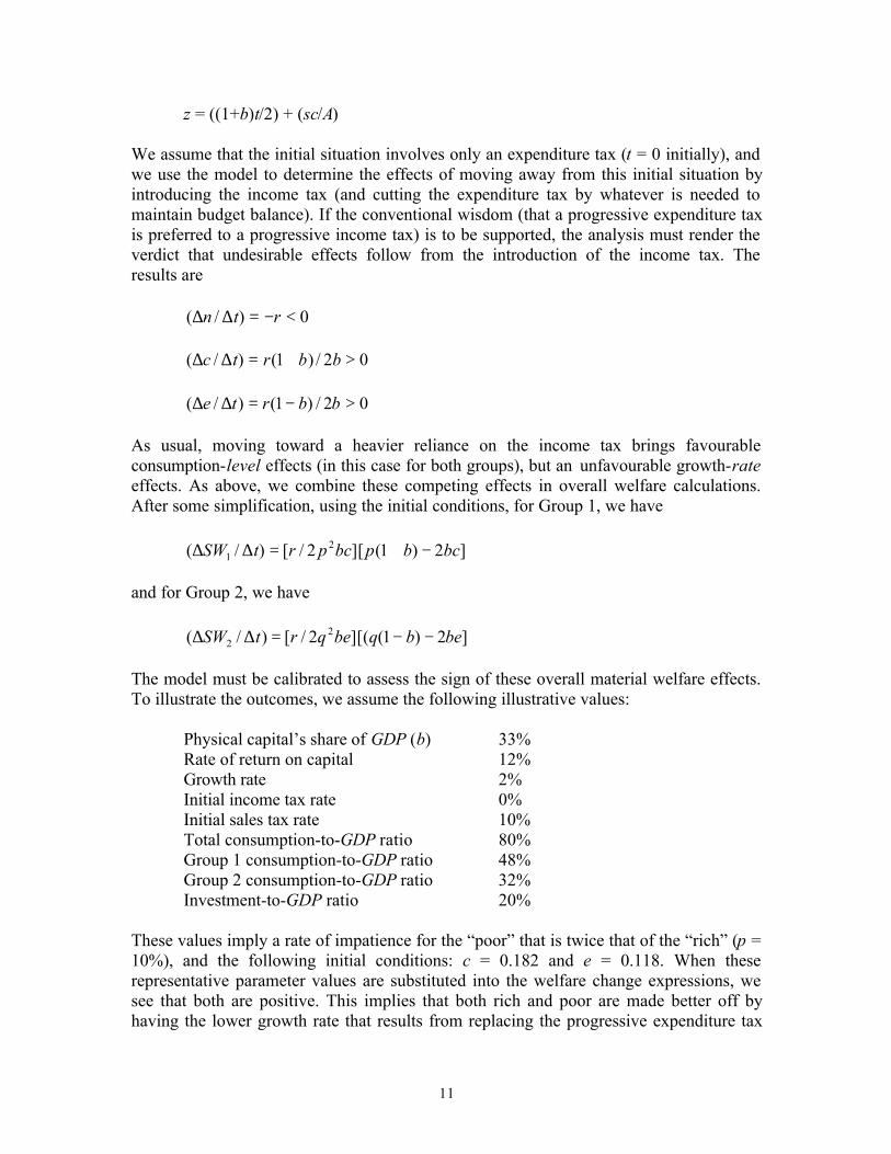
z = ((1+b)t/2) + (sc/A)

We assume that the initial situation involves only an expenditure tax (t = 0 initially), andwe use the model to determine the effects of moving away from this initial situation byintroducing the income tax (and cutting the expenditure tax by whatever is needed tomaintain budget balance). If the conventional wisdom (that a progressive expenditure taxis preferred to a progressive income tax) is to be supported, the analysis must render theverdict that undesirable effects follow from the introduction of the income tax. Theresults are

0)/( <−=∆∆ rtn

02/)1()/( >+=∆∆ bbrtc

02/)1()/( >−=∆∆ bbrte

As usual, moving toward a heavier reliance on the income tax brings favourableconsumption-level effects (in this case for both groups), but an unfavourable growth-rateeffects. As above, we combine these competing effects in overall welfare calculations.After some simplification, using the initial conditions, for Group 1, we have

]2)1(][2/[)/( 21 bcbpbcprtSW −+=∆∆

and for Group 2, we have

]2)1(][(2/[)/( 22 bebqbeqrtSW −−=∆∆

The model must be calibrated to assess the sign of these overall material welfare effects.To illustrate the outcomes, we assume the following illustrative values:

Physical capital’s share of GDP (b) 33%Rate of return on capital 12%Growth rate 2%Initial income tax rate 0%Initial sales tax rate 10%Total consumption-to-GDP ratio 80%Group 1 consumption-to-GDP ratio 48%Group 2 consumption-to-GDP ratio 32%Investment-to-GDP ratio 20%

These values imply a rate of impatience for the “poor” that is twice that of the “rich” (p =10%), and the following initial conditions: c = 0.182 and e = 0.118. When theserepresentative parameter values are substituted into the welfare change expressions, wesee that both are positive. This implies that both rich and poor are made better off byhaving the lower growth rate that results from replacing the progressive expenditure tax

12

with the progressive income tax. While other calibrations might lead to the oppositeconclusion, and this additional quantitative analysis needs to be done and reported in thenext draft of the paper, we can surely conclude that, at the very least, there is limitedsupport for conventional wisdom.

The intuition behind this finding runs as follows. From the selfish perspective of the rich,the optimal transfer to the poor is zero. Thus, with a positive transfer, the government is“too big,” and since this problem is a constant proportion of a growing GDP, less growthis preferred. This is another application of the general principle that emerged in Section 2of the paper. Finally, as far as the poor are concerned, in this illustrative calibration, theyare impatient enough to prefer the favourable consumption-level effect that accompaniesthe shift to the income tax.

4. Conclusions

The simplest version of standard growth theory does not provide a solid basis for thecommon propositions that have been advanced by many policy analysts. The standardadvice is that the income tax should be replaced by an expenditure tax (whether or notthese taxes are progressive). Since our analysis does not support these propositions, andsince it is an entirely standard version of endogenous growth theory, the results representa challenge for policy analysts – to clarify the analytical underpinnings of their advice.

13

Appendix

For the section 2 analysis, the household optimization involves maximizing

∫∞ −+

0]ln[ln dteGfC pt

subject to

sCKtrKC −−=+ )1(&

by choosing C and K. The first-order conditions can be derived by standard methods.They have been written in a more user-friendly discrete-time format in the text. Note thatthe formal derivation does not require the approximation that was part of the intuitivediscussion in the text.

Again, for the section 2 analysis, the social welfare function is the utility function of therepresentative household:

∫∞ −+=

0.]ln[ln dteGfCSW pt

We know that ntt eCC 0= and that nt

t eGG 0= so the social welfare expression can besimplified to

∫∞ −+++=000 .)ln()1(]/)ln[(ln dteefpGfCSW ptnt

The integral in this last equation can be re-expressed as ∫ − ,dtten pt and this, in turn, can

be simplified by using the standard formula ∫ ∫−= ,vduuvudv to yield

∫ ∞−− +−=−+− .]/)1[(])[/1( 02pptedtetp ptpt

When this solution is evaluated at the extreme points in time, and the result is substitutedinto the expression for SW, equation (8a) in the text is the result. When differentiatingthat equation with respect to the tax rate, we use ,/ KCc = which implies that

dtcdcdtCdC /)/()/( 00 = since K cannot jump ( 0K is independent of policy). Also,

since ,00 grKG = we know that 0/0 =dtdG as well.

The rfcg /* = result emerges from maximizing SW subject to the resource constraint,that is, by evaluating .0/ =dGdSW

The derivations for section 3 of the paper follow in a similar fashion.

14

References

Barro, R. and Sala-i-Martin, X. Economic Growth (New York: McGraw Hill) 1995.

Kesselman, J., Tax Design for a Northern Tiger, Institute for Research on Public Policy,Choices 10 (March 2004) www.irpp.org/research/index.htm

Lucas, R., “On the Mechanics of Economic Development,” Journal of MonetaryEconomics 22 (1988), 3-42.

Mankiw, G., “The Savers-Spenders Theory of Fiscal Policy,” American EconomicReview, Papers and Proceedings 90 (May 2000), 120-125.

Mintz, J., Most Favored Nation: Building a Framework for Smart Economic Policy(Toronto: C.D. Howe Institute) 2001 www.cdhowe.org/pdf/mintz_nation.pdf

Ramsey, F., “A Mathematical Theory of Saving,” Economic Journal 38 (1928) 543-549.