Embed Size (px)
Citation preview

Progress in Nuclear Magnetic Resonance Spectroscopy 57 (2010) 241–292
Contents lists available at ScienceDirect
Progress in Nuclear Magnetic Resonance Spectroscopy
journal homepage: www.elsevier .com/locate /pnmrs
Single-scan multidimensional magnetic resonance
Assaf Tal, Lucio Frydman *
The Department of Chemical Physics, Weizmann Institute of Science, Israel
a r t i c l e i n f o
Article history:Received 22 January 2010Accepted 23 March 2010Available online 22 April 2010
0079-6565/$ - see front matter � 2010 Elsevier B.V. Adoi:10.1016/j.pnmrs.2010.04.001
* Corresponding author. Tel.: +972 8 9344903; fax:E-mail address: [email protected] (L.
� 2010 Elsevier B.V. All rights reserved.
Contents
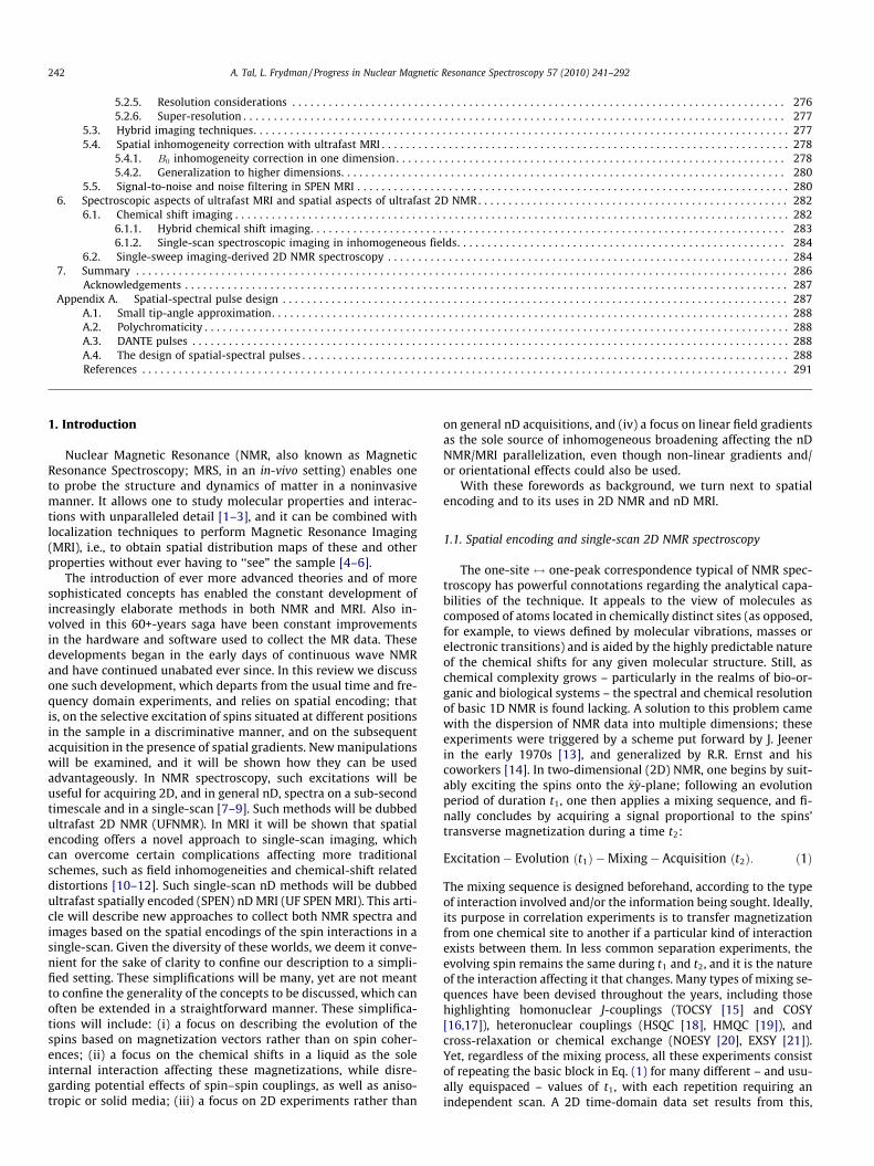
1. Introduction . . . . . . . . . . . . . . . . . . . . . . . . . . . . . . . . . . . . . . . . . . . . . . . . . . . . . . . . . . . . . . . . . . . . . . . . . . . . . . . . . . . . . . . . . . . . . . . . . . . . . . . . . 242
1.1. Spatial encoding and single-scan 2D NMR spectroscopy . . . . . . . . . . . . . . . . . . . . . . . . . . . . . . . . . . . . . . . . . . . . . . . . . . . . . . . . . . . . . . . . 2422. Elements of spatial encoding. . . . . . . . . . . . . . . . . . . . . . . . . . . . . . . . . . . . . . . . . . . . . . . . . . . . . . . . . . . . . . . . . . . . . . . . . . . . . . . . . . . . . . . . . . . . 244
2.1. The effect of spatial field gradients in NMR . . . . . . . . . . . . . . . . . . . . . . . . . . . . . . . . . . . . . . . . . . . . . . . . . . . . . . . . . . . . . . . . . . . . . . . . . . 2442.2. Chirped excitation pulses . . . . . . . . . . . . . . . . . . . . . . . . . . . . . . . . . . . . . . . . . . . . . . . . . . . . . . . . . . . . . . . . . . . . . . . . . . . . . . . . . . . . . . . . . 2452.2.1. The spins’ response to chirped excitation pulses . . . . . . . . . . . . . . . . . . . . . . . . . . . . . . . . . . . . . . . . . . . . . . . . . . . . . . . . . . . . . . . 246
2.3. Chirped storage pulses . . . . . . . . . . . . . . . . . . . . . . . . . . . . . . . . . . . . . . . . . . . . . . . . . . . . . . . . . . . . . . . . . . . . . . . . . . . . . . . . . . . . . . . . . . . 2472.4. Chirped �-pulses . . . . . . . . . . . . . . . . . . . . . . . . . . . . . . . . . . . . . . . . . . . . . . . . . . . . . . . . . . . . . . . . . . . . . . . . . . . . . . . . . . . . . . . . . . . . . . . . 2493. Single-scan ultrafast 2D NMR . . . . . . . . . . . . . . . . . . . . . . . . . . . . . . . . . . . . . . . . . . . . . . . . . . . . . . . . . . . . . . . . . . . . . . . . . . . . . . . . . . . . . . . . . . . 250
3.1. Approaches to spatial encoding . . . . . . . . . . . . . . . . . . . . . . . . . . . . . . . . . . . . . . . . . . . . . . . . . . . . . . . . . . . . . . . . . . . . . . . . . . . . . . . . . . . . 250� �3.1.1. Indirect-domain encoding with phase modulation �2 � � . . . . . . . . . . . . . . . . . . . . . . . . . . . . . . . . . . . . . . . . . . . . . . . . . . . . . . . 251
3.1.2. Indirect-domain encoding with amplitude modulation �2 � �
2
� �. . . . . . . . . . . . . . . . . . . . . . . . . . . . . . . . . . . . . . . . . . . . . . . . . . . . 251
3.1.3. Indirect-domain constant-time encoding ð�� �Þ . . . . . . . . . . . . . . . . . . . . . . . . . . . . . . . . . . . . . . . . . . . . . . . . . . . . . . . . . . . . . . . 2523.1.4. Advantages and disadvantages of each method . . . . . . . . . . . . . . . . . . . . . . . . . . . . . . . . . . . . . . . . . . . . . . . . . . . . . . . . . . . . . . . . 253
3.2. Decoding the information: 2D signals in a single acquisition . . . . . . . . . . . . . . . . . . . . . . . . . . . . . . . . . . . . . . . . . . . . . . . . . . . . . . . . . . . . 253
3.2.1. Spatial-spectral acquisition of spatially-encoded NMR interactions . . . . . . . . . . . . . . . . . . . . . . . . . . . . . . . . . . . . . . . . . . . . . . . . 2533.2.2. Mathematical formulation of the gradient-driven decoding . . . . . . . . . . . . . . . . . . . . . . . . . . . . . . . . . . . . . . . . . . . . . . . . . . . . . . 2553.3. Practical considerations in ultrafast 2D NMR . . . . . . . . . . . . . . . . . . . . . . . . . . . . . . . . . . . . . . . . . . . . . . . . . . . . . . . . . . . . . . . . . . . . . . . . . 257
3.3.1. Spectral characteristics. . . . . . . . . . . . . . . . . . . . . . . . . . . . . . . . . . . . . . . . . . . . . . . . . . . . . . . . . . . . . . . . . . . . . . . . . . . . . . . . . . . . 2573.3.2. Practical aspects of spatial encoding . . . . . . . . . . . . . . . . . . . . . . . . . . . . . . . . . . . . . . . . . . . . . . . . . . . . . . . . . . . . . . . . . . . . . . . . . 2583.3.3. Line shape considerations . . . . . . . . . . . . . . . . . . . . . . . . . . . . . . . . . . . . . . . . . . . . . . . . . . . . . . . . . . . . . . . . . . . . . . . . . . . . . . . . . 2583.3.4. Signal to noise . . . . . . . . . . . . . . . . . . . . . . . . . . . . . . . . . . . . . . . . . . . . . . . . . . . . . . . . . . . . . . . . . . . . . . . . . . . . . . . . . . . . . . . . . . 2603.3.5. A formal view of EPSI . . . . . . . . . . . . . . . . . . . . . . . . . . . . . . . . . . . . . . . . . . . . . . . . . . . . . . . . . . . . . . . . . . . . . . . . . . . . . . . . . . . . . 2623.3.6. Examples . . . . . . . . . . . . . . . . . . . . . . . . . . . . . . . . . . . . . . . . . . . . . . . . . . . . . . . . . . . . . . . . . . . . . . . . . . . . . . . . . . . . . . . . . . . . . . . 2634. Spatial-spectral single-scan spectroscopy. . . . . . . . . . . . . . . . . . . . . . . . . . . . . . . . . . . . . . . . . . . . . . . . . . . . . . . . . . . . . . . . . . . . . . . . . . . . . . . . . . 263
4.1. Conventional Hadamard spectroscopy: a review . . . . . . . . . . . . . . . . . . . . . . . . . . . . . . . . . . . . . . . . . . . . . . . . . . . . . . . . . . . . . . . . . . . . . . 2634.1.1. Complex Hadamard matrices. . . . . . . . . . . . . . . . . . . . . . . . . . . . . . . . . . . . . . . . . . . . . . . . . . . . . . . . . . . . . . . . . . . . . . . . . . . . . . . 264
4.2. Single-scan Hadamard spectroscopy . . . . . . . . . . . . . . . . . . . . . . . . . . . . . . . . . . . . . . . . . . . . . . . . . . . . . . . . . . . . . . . . . . . . . . . . . . . . . . . . 2644.3. Signal-to-noise considerations . . . . . . . . . . . . . . . . . . . . . . . . . . . . . . . . . . . . . . . . . . . . . . . . . . . . . . . . . . . . . . . . . . . . . . . . . . . . . . . . . . . . . 2664.4. The general case of spatial-spectral single-scan 2D NMR. . . . . . . . . . . . . . . . . . . . . . . . . . . . . . . . . . . . . . . . . . . . . . . . . . . . . . . . . . . . . . . . 2665. Single-scan nD spatially-encoded imaging (SPEN MRI) . . . . . . . . . . . . . . . . . . . . . . . . . . . . . . . . . . . . . . . . . . . . . . . . . . . . . . . . . . . . . . . . . . . . . . . 268
5.1. nD NMR imaging . . . . . . . . . . . . . . . . . . . . . . . . . . . . . . . . . . . . . . . . . . . . . . . . . . . . . . . . . . . . . . . . . . . . . . . . . . . . . . . . . . . . . . . . . . . . . . . . 2695.2. Principles of spatially encoded MRI . . . . . . . . . . . . . . . . . . . . . . . . . . . . . . . . . . . . . . . . . . . . . . . . . . . . . . . . . . . . . . . . . . . . . . . . . . . . . . . . . 2715.2.1. SPEN MRI and the stationary phase approximation . . . . . . . . . . . . . . . . . . . . . . . . . . . . . . . . . . . . . . . . . . . . . . . . . . . . . . . . . . . . . 2725.2.2. Stationary points and SPEN MRI . . . . . . . . . . . . . . . . . . . . . . . . . . . . . . . . . . . . . . . . . . . . . . . . . . . . . . . . . . . . . . . . . . . . . . . . . . . . 2735.2.3. Example #1: 1D spatially-encoded imaging . . . . . . . . . . . . . . . . . . . . . . . . . . . . . . . . . . . . . . . . . . . . . . . . . . . . . . . . . . . . . . . . . . . 2745.2.4. Example #2: 2D SPEN MRI . . . . . . . . . . . . . . . . . . . . . . . . . . . . . . . . . . . . . . . . . . . . . . . . . . . . . . . . . . . . . . . . . . . . . . . . . . . . . . . . 274
ll rights reserved.
+972 8 9344123.Frydman).
242 A. Tal, L. Frydman / Progress in Nuclear Magnetic Resonance Spectroscopy 57 (2010) 241–292
5.2.5. Resolution considerations . . . . . . . . . . . . . . . . . . . . . . . . . . . . . . . . . . . . . . . . . . . . . . . . . . . . . . . . . . . . . . . . . . . . . . . . . . . . . . . . . 2765.2.6. Super-resolution . . . . . . . . . . . . . . . . . . . . . . . . . . . . . . . . . . . . . . . . . . . . . . . . . . . . . . . . . . . . . . . . . . . . . . . . . . . . . . . . . . . . . . . . . 277
5.3. Hybrid imaging techniques. . . . . . . . . . . . . . . . . . . . . . . . . . . . . . . . . . . . . . . . . . . . . . . . . . . . . . . . . . . . . . . . . . . . . . . . . . . . . . . . . . . . . . . . 2775.4. Spatial inhomogeneity correction with ultrafast MRI . . . . . . . . . . . . . . . . . . . . . . . . . . . . . . . . . . . . . . . . . . . . . . . . . . . . . . . . . . . . . . . . . . . 278
5.4.1. B0 inhomogeneity correction in one dimension . . . . . . . . . . . . . . . . . . . . . . . . . . . . . . . . . . . . . . . . . . . . . . . . . . . . . . . . . . . . . . . . 2785.4.2. Generalization to higher dimensions. . . . . . . . . . . . . . . . . . . . . . . . . . . . . . . . . . . . . . . . . . . . . . . . . . . . . . . . . . . . . . . . . . . . . . . . . 280
5.5. Signal-to-noise and noise filtering in SPEN MRI . . . . . . . . . . . . . . . . . . . . . . . . . . . . . . . . . . . . . . . . . . . . . . . . . . . . . . . . . . . . . . . . . . . . . . . 280
6. Spectroscopic aspects of ultrafast MRI and spatial aspects of ultrafast 2D NMR . . . . . . . . . . . . . . . . . . . . . . . . . . . . . . . . . . . . . . . . . . . . . . . . . . . 2826.1. Chemical shift imaging . . . . . . . . . . . . . . . . . . . . . . . . . . . . . . . . . . . . . . . . . . . . . . . . . . . . . . . . . . . . . . . . . . . . . . . . . . . . . . . . . . . . . . . . . . . 282
6.1.1. Hybrid chemical shift imaging. . . . . . . . . . . . . . . . . . . . . . . . . . . . . . . . . . . . . . . . . . . . . . . . . . . . . . . . . . . . . . . . . . . . . . . . . . . . . . 2836.1.2. Single-scan spectroscopic imaging in inhomogeneous fields. . . . . . . . . . . . . . . . . . . . . . . . . . . . . . . . . . . . . . . . . . . . . . . . . . . . . . 2846.2. Single-sweep imaging-derived 2D NMR spectroscopy . . . . . . . . . . . . . . . . . . . . . . . . . . . . . . . . . . . . . . . . . . . . . . . . . . . . . . . . . . . . . . . . . . 284
7. Summary . . . . . . . . . . . . . . . . . . . . . . . . . . . . . . . . . . . . . . . . . . . . . . . . . . . . . . . . . . . . . . . . . . . . . . . . . . . . . . . . . . . . . . . . . . . . . . . . . . . . . . . . . . . 286Acknowledgements . . . . . . . . . . . . . . . . . . . . . . . . . . . . . . . . . . . . . . . . . . . . . . . . . . . . . . . . . . . . . . . . . . . . . . . . . . . . . . . . . . . . . . . . . . . . . . . . . . . 287Appendix A. Spatial-spectral pulse design . . . . . . . . . . . . . . . . . . . . . . . . . . . . . . . . . . . . . . . . . . . . . . . . . . . . . . . . . . . . . . . . . . . . . . . . . . . . . . . . . . . 287
A.1. Small tip-angle approximation. . . . . . . . . . . . . . . . . . . . . . . . . . . . . . . . . . . . . . . . . . . . . . . . . . . . . . . . . . . . . . . . . . . . . . . . . . . . . . . . . . . . . 288A.2. Polychromaticity . . . . . . . . . . . . . . . . . . . . . . . . . . . . . . . . . . . . . . . . . . . . . . . . . . . . . . . . . . . . . . . . . . . . . . . . . . . . . . . . . . . . . . . . . . . . . . . . 288A.3. DANTE pulses . . . . . . . . . . . . . . . . . . . . . . . . . . . . . . . . . . . . . . . . . . . . . . . . . . . . . . . . . . . . . . . . . . . . . . . . . . . . . . . . . . . . . . . . . . . . . . . . . . 288A.4. The design of spatial-spectral pulses . . . . . . . . . . . . . . . . . . . . . . . . . . . . . . . . . . . . . . . . . . . . . . . . . . . . . . . . . . . . . . . . . . . . . . . . . . . . . . . . 288
References . . . . . . . . . . . . . . . . . . . . . . . . . . . . . . . . . . . . . . . . . . . . . . . . . . . . . . . . . . . . . . . . . . . . . . . . . . . . . . . . . . . . . . . . . . . . . . . . . . . . . . . . . . 2911. Introduction
Nuclear Magnetic Resonance (NMR, also known as MagneticResonance Spectroscopy; MRS, in an in-vivo setting) enables oneto probe the structure and dynamics of matter in a noninvasivemanner. It allows one to study molecular properties and interac-tions with unparalleled detail [1–3], and it can be combined withlocalization techniques to perform Magnetic Resonance Imaging(MRI), i.e., to obtain spatial distribution maps of these and otherproperties without ever having to ‘‘see” the sample [4–6].
The introduction of ever more advanced theories and of moresophisticated concepts has enabled the constant development ofincreasingly elaborate methods in both NMR and MRI. Also in-volved in this 60+-years saga have been constant improvementsin the hardware and software used to collect the MR data. Thesedevelopments began in the early days of continuous wave NMRand have continued unabated ever since. In this review we discussone such development, which departs from the usual time and fre-quency domain experiments, and relies on spatial encoding; thatis, on the selective excitation of spins situated at different positionsin the sample in a discriminative manner, and on the subsequentacquisition in the presence of spatial gradients. New manipulationswill be examined, and it will be shown how they can be usedadvantageously. In NMR spectroscopy, such excitations will beuseful for acquiring 2D, and in general nD, spectra on a sub-secondtimescale and in a single-scan [7–9]. Such methods will be dubbedultrafast 2D NMR (UFNMR). In MRI it will be shown that spatialencoding offers a novel approach to single-scan imaging, whichcan overcome certain complications affecting more traditionalschemes, such as field inhomogeneities and chemical-shift relateddistortions [10–12]. Such single-scan nD methods will be dubbedultrafast spatially encoded (SPEN) nD MRI (UF SPEN MRI). This arti-cle will describe new approaches to collect both NMR spectra andimages based on the spatial encodings of the spin interactions in asingle-scan. Given the diversity of these worlds, we deem it conve-nient for the sake of clarity to confine our description to a simpli-fied setting. These simplifications will be many, yet are not meantto confine the generality of the concepts to be discussed, which canoften be extended in a straightforward manner. These simplifica-tions will include: (i) a focus on describing the evolution of thespins based on magnetization vectors rather than on spin coher-ences; (ii) a focus on the chemical shifts in a liquid as the soleinternal interaction affecting these magnetizations, while disre-garding potential effects of spin–spin couplings, as well as aniso-tropic or solid media; (iii) a focus on 2D experiments rather than
on general nD acquisitions, and (iv) a focus on linear field gradientsas the sole source of inhomogeneous broadening affecting the nDNMR/MRI parallelization, even though non-linear gradients and/or orientational effects could also be used.
With these forewords as background, we turn next to spatialencoding and to its uses in 2D NMR and nD MRI.
1.1. Spatial encoding and single-scan 2D NMR spectroscopy
The one-site $ one-peak correspondence typical of NMR spec-troscopy has powerful connotations regarding the analytical capa-bilities of the technique. It appeals to the view of molecules ascomposed of atoms located in chemically distinct sites (as opposed,for example, to views defined by molecular vibrations, masses orelectronic transitions) and is aided by the highly predictable natureof the chemical shifts for any given molecular structure. Still, aschemical complexity grows – particularly in the realms of bio-or-ganic and biological systems – the spectral and chemical resolutionof basic 1D NMR is found lacking. A solution to this problem camewith the dispersion of NMR data into multiple dimensions; theseexperiments were triggered by a scheme put forward by J. Jeenerin the early 1970s [13], and generalized by R.R. Ernst and hiscoworkers [14]. In two-dimensional (2D) NMR, one begins by suit-ably exciting the spins onto the xy-plane; following an evolutionperiod of duration t1, one then applies a mixing sequence, and fi-nally concludes by acquiring a signal proportional to the spins’transverse magnetization during a time t2:
Excitation� Evolution ðt1Þ �Mixing� Acquisition ðt2Þ: ð1Þ
The mixing sequence is designed beforehand, according to the typeof interaction involved and/or the information being sought. Ideally,its purpose in correlation experiments is to transfer magnetizationfrom one chemical site to another if a particular kind of interactionexists between them. In less common separation experiments, theevolving spin remains the same during t1 and t2, and it is the natureof the interaction affecting it that changes. Many types of mixing se-quences have been devised throughout the years, including thosehighlighting homonuclear J-couplings (TOCSY [15] and COSY[16,17]), heteronuclear couplings (HSQC [18], HMQC [19]), andcross-relaxation or chemical exchange (NOESY [20], EXSY [21]).Yet, regardless of the mixing process, all these experiments consistof repeating the basic block in Eq. (1) for many different – and usu-ally equispaced – values of t1, with each repetition requiring anindependent scan. A 2D time-domain data set results from this,

A. Tal, L. Frydman / Progress in Nuclear Magnetic Resonance Spectroscopy 57 (2010) 241–292 243
and is subsequently Fourier transformed along both the t1 and t2
dimensions to yield the two-dimensional spectrum being sought.A drawback of this otherwise extremely powerful data acquisi-
tion approach is that the acquisition time it involves may end upbeing dictated by sampling rather than by sensitivity consider-ations. Moreover, since for maximizing the steady-state responseof the t1 series one must wait a time � T1 before repeating theexperiment with a different t1 value, the acquisition of a full 2Dspectrum may take minutes, solely on the basis of the indirect-do-main sampling considerations. This problem gets exponentiallycompounded as the dimensionality of the experiment increases,and its compensation has been the subject of extensive efforts overthe last years. Indeed, the reduction of such long experimentaltimes would be highly beneficial not just from the practical acqui-sition-time point of view, but also from a fundamental one: longacquisition processes preclude one from monitoring many pro-cesses and/or unstable systems, which would otherwise beammenable to nD NMR. These include monitoring the dynamicsof reactions which occur on short time scales, such as protein fold-ing or chemical exchange reactions of chemically unstable biomol-ecules, and the use of metastable spin states, such as those arisingfrom hyperpolarization procedures.
The multi-scan nature of nD NMR was found particularly con-fining within the context of MRI, which is an inherently multidi-mensional experiment carried out on a sample with amplesensitivity. Proposals that have been made over the years to reducethe minimal number of scans required to collect the nD NMR/MRIdata include departing from fast Fourier transform (FT) algorithmsand relying instead on techniques such as non-linear sampling,maximum entropy, projection-reconstruction or least square fit-ting procedures to bypass the typical Nyquist-imposed samplingcriteria. Proposals also include the use of small angle excitations
Fig. 1. Above: outline of a conventional 2D NMR experiment. A 1D experiment is repmagnetic resonance spectroscopy (UF2DNMR). Instead of executing N experiments sexperiments, each with a different t1 value, are carried out in parallel. A suitable acquisiused to recover the Free Induction Decay (FID) from each slice, once again simultaneou
and/or other relaxation-enhancement means to shorten to a mini-mum the time intervals between scans, as well as reliance on mul-tiple receivers. Still, the most dramatic reduction in the timerequired by experiments came with Mansfield’s introduction ofEcho Planar Imaging (EPI), which exploits the man-made, gradi-ent-driven nature of the spin interactions arising in MRI to sampleentire volumes of the relevant time-domain within a single-scan,as a function of a single acquisition time, t. This extremely power-ful concept enabled - among other developments - the advent ofreal-time, functional MRI. However, its generalization to the acqui-sition of arbitrary configurations, involving chemical shifts and/orJ-couplings which cannot be dictated ‘‘at will”, has proven muchmore elusive.
Still, it was shown in 2002 that a dramatic reduction in thenumber of scans required by any nD NMR/MRI experiments couldbe achieved, if the canonical Jeener–Ernst paradigm of serial time-domain multi-scan encodings were replaced by an analogous butparallel idea [8]: instead of performing N1 experiments sequen-tially in time, increasing the value of t1 with each increment, thesample could be spatially partitioned into spatial elements, and adifferent t1 value ascribed to the different partitions. This spatialencoding is a process that can actually be imparted in a single,one-shot fashion. Acquiring the signals originating from the vari-ous positions could result in the retrieval of an otherwise conven-tional spectrum, but in a single-scan. This is the route taken by so-called spatially encoded ultrafast (UF) nD NMR spectroscopy, andby related nD MRI localization methods (Fig. 1).
The upcoming sections will address numerous aspects of theseexperiments, including how to partition the sample into slices,how to spatially encode arbitrary X1 couplings, and how to exploitthe position-dependent FIDs to retrieve 2D spectra and images in asingle-scan. Before doing so, however, we deem it convenient to
eated N times, each time varying the evolution time t1. Below: spatially encodedequentially, the sample is spatially partitioned into slices. A set of N differenttion method capable of probing the magnetization as a function of position is thensly. Thus, it is possible to complete a full 2D NMR acquisition within a single-scan.

z z z
(a) (b) (c)
ApplyGradient, GExcite( 2
π
Time τ
)
Fig. 2. The effect of a z-gradient, G ¼ Gz. (a) The spins, initially in thermal equilibrium, point in the direction of the field. They are then excited onto the xy-plane (b) using ahard p
2-pulse. (c) The application of a gradient G for a time s will cause spins at different positions to precess at different rates, effectively winding them along the z-axis. Notethat chemical shift evolution is not taken into account in this figure.
244 A. Tal, L. Frydman / Progress in Nuclear Magnetic Resonance Spectroscopy 57 (2010) 241–292
introduce a discussion of the effect of linear field gradients – a to-pic of central importance in contemporary NMR and MRI in gen-eral, and in UF 2D NMR/MRI in particular.
2. Elements of spatial encoding
One of the main ingredients involved in the spatial encoding ofthe indirect-domain interactions is the joint application of fieldgradients and of frequency-swept pulses. After defining the actionof a gradient, this section will elaborate upon the use of pulseswhose frequencies are swept linearly in time – also known aschirped pulses [22,23]. Specifically, it will be shown how theycan be used to excite, store and flip the spins of the sample sequen-tially in time and space, and how this can ultimately lead to a dif-ferent effective t1 value in each physical portion of the sample.
2.1. The effect of spatial field gradients in NMR
When a sample is placed in a homogeneous magnetic field1
B ¼ B0z, the spins in the sample precess about the main field. Differ-ent spins will precess at slightly different frequencies, cðB0 þ DB0Þ �xL þ Dx, where c is a nucleus-dependent constant known as thegyromagnetic ratio of the nucleus; xL ¼ cB0 is the Larmor frequency;and Dx ¼ cDB0 is a small quantity which depends on the precisechemical environment of the spins as is given by their chemical shift.The xL term is shared by all spins of a particular species, and can beaccounted for using the so-called rotating frame transformation;hence, in what follows, xL will be omitted. Furthermore, a single,particular chemical shift, Dx ¼ X1, will be the focus of the presentanalysis.
Linear magnetic field gradients induce a small distortion of thenuclear precession frequencies, which vary linearly throughout thesample along the gradient’s direction. Mathematically, these fieldvariations are described by a vector G, specified in units of fieldper unit length (e.g., Gauss per centimeter, milli-Tesla per meter,etc). The overall precession frequency in the rotating frame inthe presence of such a gradient will be given, for a particular chem-
1 It is important at this point to make a distinction between two sets of coordinatesused in NMR. The physical, Cartesian coordinates of real space will be marked ðx; y; zÞ,while the rotating frame of spin-space, wherein the magnetization vectors evolve,will be marked by ðx; y; zÞ. These two systems can be considered independent of eachother [24].
ical site, by a superposition of the chemical shift X1 and an addi-tional term, cG � r:
xðr; tÞ ¼ X1 þ cGðtÞ � r: ð2Þ
Most NMR/MRI spectrometers allow one to vary the gradient, G, as afunction of time, and hence a time-dependence has been noted inEq. (2).
Fig. 2 illustrates the evolution induced by a pulsed DC gradientalong the z-axis, G ¼ Gz, following a p
2 excitation pulse. The spins,initially in thermal equilibrium along the Bloch sphere’s z-axis,are thus tipped onto the xy plane. Following this, each spinprecesses with a frequency proportional to its position, xðzÞ ¼X1 þ cGz. Pictorially, the effect of such pulsing and constant gradi-ent combination can be described as a winding of the spins(Fig. 2c), as for a given time interval s, each spin has precessedby a different angle, depending on its z-coordinate. One can alsodescribe this evolution as inducing a dephasing of the bulk signal:since the NMR/MRI experiment monitors a vectorial sum over allspins in a sample, the signal from an ensemble of spins facing dif-ferent directions adds up destructively. Indeed, a spin at position rwill, under the influence of a general time-dependent gradient GðtÞacting between times t1 and t2, acquire a phase D/G given by:
D/Gðr; t1; t2Þ ¼Z t2
t1
xðr; t0Þdt0 ¼ cZ t2
t1
Gðt0Þ � rdt0: ð3Þ
It is often customary to introduce the notation:
kðtÞ ¼ cZ t
t1
Gðt0Þdt0: ð4Þ
by which the acquired phase due to the gradient in the time intervalt0 2 ½t1; t2� can be written:
D/Gðr; tÞ ¼ kðtÞ � r: ð5Þ
This notation draws out the Fourier conjugacy of the variables r andk, similar to the conjugacy between time and frequency in usualpulsed NMR experiments. This also suggests that monitoring NMRsignals over an array of k-values and Fourier transforming the ac-quired data will deliver spatially-dependent information. To visual-ize this, we can describe the magnetization as:
Mðr; tÞ / q0ðrÞ cosðkðtÞ � rÞxþ sinðkðtÞ � rÞyð Þ� Mxðr; tÞxþMyðr; tÞy: ð6Þ
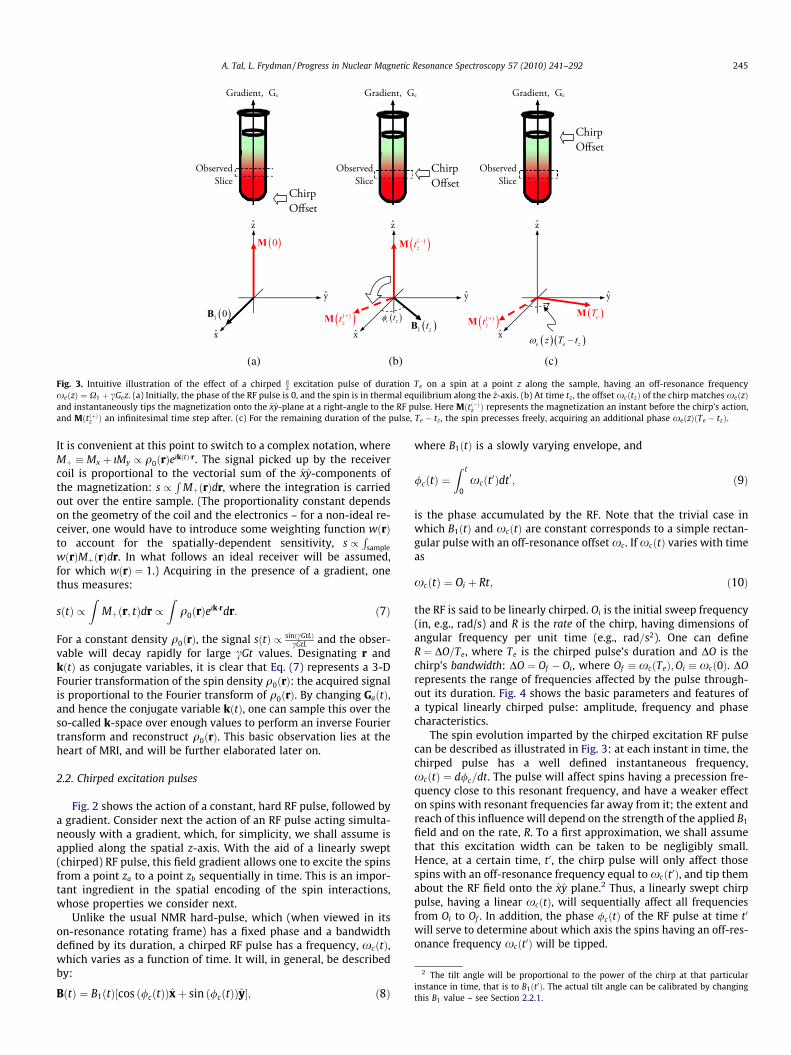
Fig. 3. Intuitive illustration of the effect of a chirped p2 excitation pulse of duration Te on a spin at a point z along the sample, having an off-resonance frequency
xeðzÞ ¼ X1 þ cGez. (a) Initially, the phase of the RF pulse is 0, and the spin is in thermal equilibrium along the z-axis. (b) At time tz , the offset xcðtzÞ of the chirp matches xeðzÞand instantaneously tips the magnetization onto the xy-plane at a right-angle to the RF pulse. Here Mðtð�Þz Þ represents the magnetization an instant before the chirp’s action,and MðtðþÞz Þ an infinitesimal time step after. (c) For the remaining duration of the pulse, Te � tz , the spin precesses freely, acquiring an additional phase xeðzÞðTe � tzÞ.
2 The tilt angle will be proportional to the power of the chirp at that particularinstance in time, that is to B1ðt0Þ. The actual tilt angle can be calibrated by changingthis B1 value – see Section 2.2.1.
A. Tal, L. Frydman / Progress in Nuclear Magnetic Resonance Spectroscopy 57 (2010) 241–292 245
It is convenient at this point to switch to a complex notation, whereMþ � Mx þ ıMy / q0ðrÞeıkðtÞ�r. The signal picked up by the receivercoil is proportional to the vectorial sum of the xy-components ofthe magnetization: s /
RMþðrÞdr, where the integration is carried
out over the entire sample. (The proportionality constant dependson the geometry of the coil and the electronics – for a non-ideal re-ceiver, one would have to introduce some weighting function wðrÞto account for the spatially-dependent sensitivity, s /
Rsample
wðrÞMþðrÞdr. In what follows an ideal receiver will be assumed,for which wðrÞ ¼ 1.) Acquiring in the presence of a gradient, onethus measures:
sðtÞ /Z
Mþðr; tÞdr /Z
q0ðrÞeık�rdr: ð7Þ
For a constant density q0ðrÞ, the signal sðtÞ / sinðcGtLÞcGtL and the obser-
vable will decay rapidly for large cGt values. Designating r andkðtÞ as conjugate variables, it is clear that Eq. (7) represents a 3-DFourier transformation of the spin density q0ðrÞ: the acquired signalis proportional to the Fourier transform of q0ðrÞ. By changing GaðtÞ,and hence the conjugate variable kðtÞ, one can sample this over theso-called k-space over enough values to perform an inverse Fouriertransform and reconstruct q0ðrÞ. This basic observation lies at theheart of MRI, and will be further elaborated later on.
2.2. Chirped excitation pulses
Fig. 2 shows the action of a constant, hard RF pulse, followed bya gradient. Consider next the action of an RF pulse acting simulta-neously with a gradient, which, for simplicity, we shall assume isapplied along the spatial z-axis. With the aid of a linearly swept(chirped) RF pulse, this field gradient allows one to excite the spinsfrom a point za to a point zb sequentially in time. This is an impor-tant ingredient in the spatial encoding of the spin interactions,whose properties we consider next.
Unlike the usual NMR hard-pulse, which (when viewed in itson-resonance rotating frame) has a fixed phase and a bandwidthdefined by its duration, a chirped RF pulse has a frequency, xcðtÞ,which varies as a function of time. It will, in general, be describedby:
BðtÞ ¼ B1ðtÞ cos /cðtÞð Þxþ sin /cðtÞð Þy½ �; ð8Þ
where B1ðtÞ is a slowly varying envelope, and
/cðtÞ ¼Z t
0xcðt0Þdt0; ð9Þ
is the phase accumulated by the RF. Note that the trivial case inwhich B1ðtÞ and xcðtÞ are constant corresponds to a simple rectan-gular pulse with an off-resonance offset xc . If xcðtÞ varies with timeas
xcðtÞ ¼ Oi þ Rt; ð10Þ
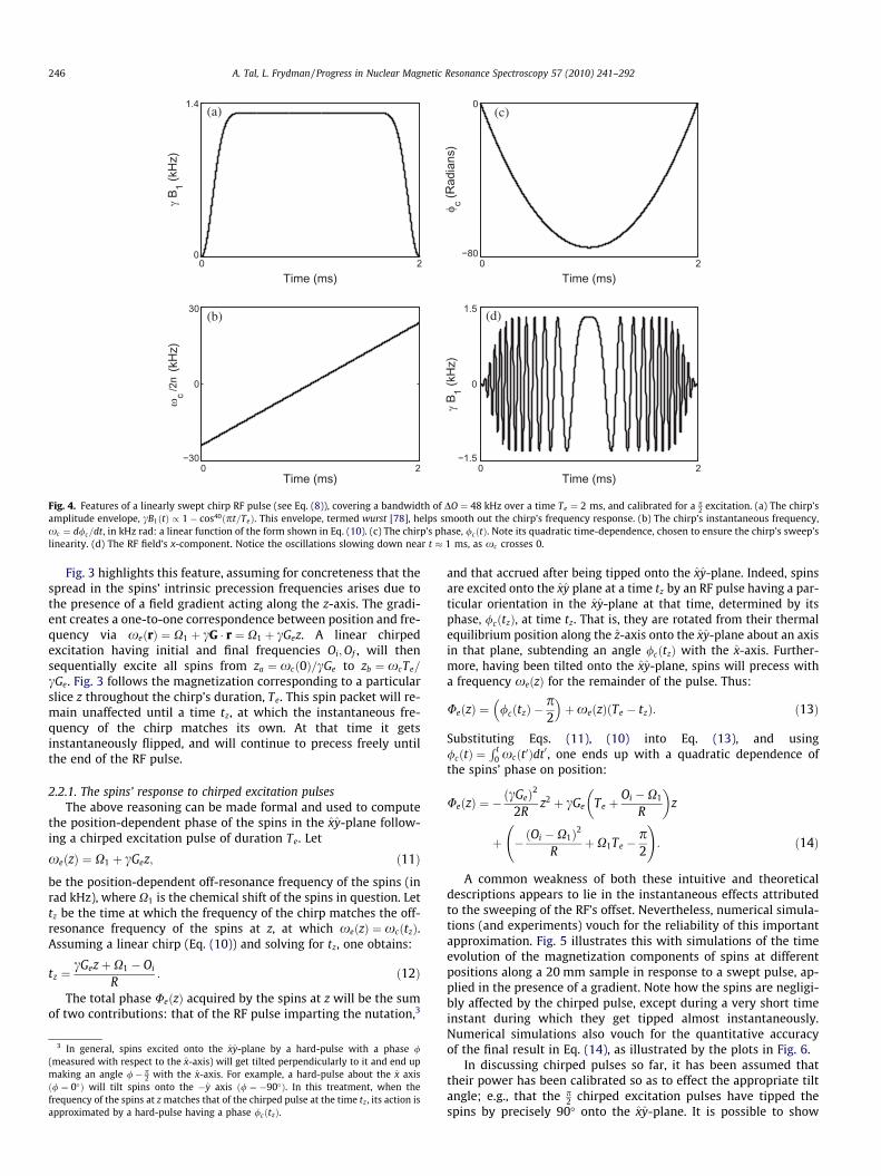
the RF is said to be linearly chirped. Oi is the initial sweep frequency(in, e.g., rad/s) and R is the rate of the chirp, having dimensions ofangular frequency per unit time (e.g., rad=s2). One can defineR ¼ DO=Te, where Te is the chirped pulse’s duration and DO is thechirp’s bandwidth: DO ¼ Of � Oi, where Of � xcðTeÞ;Oi � xcð0Þ. DOrepresents the range of frequencies affected by the pulse through-out its duration. Fig. 4 shows the basic parameters and features ofa typical linearly chirped pulse: amplitude, frequency and phasecharacteristics.
The spin evolution imparted by the chirped excitation RF pulsecan be described as illustrated in Fig. 3: at each instant in time, thechirped pulse has a well defined instantaneous frequency,xcðtÞ ¼ d/c=dt. The pulse will affect spins having a precession fre-quency close to this resonant frequency, and have a weaker effecton spins with resonant frequencies far away from it; the extent andreach of this influence will depend on the strength of the applied B1
field and on the rate, R. To a first approximation, we shall assumethat this excitation width can be taken to be negligibly small.Hence, at a certain time, t0, the chirp pulse will only affect thosespins with an off-resonance frequency equal to xcðt0Þ, and tip themabout the RF field onto the xy plane.2 Thus, a linearly swept chirppulse, having a linear xcðtÞ, will sequentially affect all frequenciesfrom Oi to Of . In addition, the phase /cðtÞ of the RF pulse at time t0
will serve to determine about which axis the spins having an off-res-onance frequency xcðt0Þ will be tipped.
0 20
1.4
Time (ms)
γ B 1 (k
Hz)
(a)
0 2−80
0
Time (ms)
φ c (Rad
ians
)
(c)
0 2−30
0
30
Time (ms)
ωc
(kH
z)
(b)
0 2−1.5
0
1.5
Time (ms)
γ B 1 (k
Hz)
(d)
/2п
Fig. 4. Features of a linearly swept chirp RF pulse (see Eq. (8)), covering a bandwidth of DO ¼ 48 kHz over a time Te ¼ 2 ms, and calibrated for a p2 excitation. (a) The chirp’s
amplitude envelope, cB1ðtÞ / 1� cos40ðpt=TeÞ. This envelope, termed wurst [78], helps smooth out the chirp’s frequency response. (b) The chirp’s instantaneous frequency,xc ¼ d/c=dt, in kHz rad: a linear function of the form shown in Eq. (10). (c) The chirp’s phase, /cðtÞ. Note its quadratic time-dependence, chosen to ensure the chirp’s sweep’slinearity. (d) The RF field’s x-component. Notice the oscillations slowing down near t � 1 ms, as xc crosses 0.
246 A. Tal, L. Frydman / Progress in Nuclear Magnetic Resonance Spectroscopy 57 (2010) 241–292
Fig. 3 highlights this feature, assuming for concreteness that thespread in the spins’ intrinsic precession frequencies arises due tothe presence of a field gradient acting along the z-axis. The gradi-ent creates a one-to-one correspondence between position and fre-quency via xeðrÞ ¼ X1 þ cG � r ¼ X1 þ cGez. A linear chirpedexcitation having initial and final frequencies Oi;Of , will thensequentially excite all spins from za ¼ xcð0Þ=cGe to zb ¼ xcTe=
cGe. Fig. 3 follows the magnetization corresponding to a particularslice z throughout the chirp’s duration, Te. This spin packet will re-main unaffected until a time tz, at which the instantaneous fre-quency of the chirp matches its own. At that time it getsinstantaneously flipped, and will continue to precess freely untilthe end of the RF pulse.
2.2.1. The spins’ response to chirped excitation pulsesThe above reasoning can be made formal and used to compute
the position-dependent phase of the spins in the xy-plane follow-ing a chirped excitation pulse of duration Te. Let
xeðzÞ ¼ X1 þ cGez; ð11Þ
be the position-dependent off-resonance frequency of the spins (inrad kHz), where X1 is the chemical shift of the spins in question. Lettz be the time at which the frequency of the chirp matches the off-resonance frequency of the spins at z, at which xeðzÞ ¼ xcðtzÞ.Assuming a linear chirp (Eq. (10)) and solving for tz, one obtains:
tz ¼cGezþX1 � Oi
R: ð12Þ
The total phase UeðzÞ acquired by the spins at z will be the sumof two contributions: that of the RF pulse imparting the nutation,3
3 In general, spins excited onto the xy-plane by a hard-pulse with a phase /(measured with respect to the x-axis) will get tilted perpendicularly to it and end upmaking an angle /� p
2 with the x-axis. For example, a hard-pulse about the x axisð/ ¼ 0�Þ will tilt spins onto the �y axis ð/ ¼ �90�Þ. In this treatment, when thefrequency of the spins at z matches that of the chirped pulse at the time tz , its action isapproximated by a hard-pulse having a phase /cðtzÞ.
and that accrued after being tipped onto the xy-plane. Indeed, spinsare excited onto the xy plane at a time tz by an RF pulse having a par-ticular orientation in the xy-plane at that time, determined by itsphase, /cðtzÞ, at time tz. That is, they are rotated from their thermalequilibrium position along the z-axis onto the xy-plane about an axisin that plane, subtending an angle /cðtzÞ with the x-axis. Further-more, having been tilted onto the xy-plane, spins will precess witha frequency xeðzÞ for the remainder of the pulse. Thus:
UeðzÞ ¼ /cðtzÞ �p2
� �þxeðzÞ Te � tzð Þ: ð13Þ
Substituting Eqs. (11), (10) into Eq. (13), and using/cðtÞ ¼
R t0 xcðt0Þdt0, one ends up with a quadratic dependence of
the spins’ phase on position:
UeðzÞ ¼ �ðcGeÞ2
2Rz2 þ cGe Te þ
Oi �X1
R
� �z
þ �ðOi �X1Þ2
RþX1Te �
p2
!: ð14Þ
A common weakness of both these intuitive and theoreticaldescriptions appears to lie in the instantaneous effects attributedto the sweeping of the RF’s offset. Nevertheless, numerical simula-tions (and experiments) vouch for the reliability of this importantapproximation. Fig. 5 illustrates this with simulations of the timeevolution of the magnetization components of spins at differentpositions along a 20 mm sample in response to a swept pulse, ap-plied in the presence of a gradient. Note how the spins are negligi-bly affected by the chirped pulse, except during a very short timeinstant during which they get tipped almost instantaneously.Numerical simulations also vouch for the quantitative accuracyof the final result in Eq. (14), as illustrated by the plots in Fig. 6.
In discussing chirped pulses so far, it has been assumed thattheir power has been calibrated so as to effect the appropriate tiltangle; e.g., that the p
2 chirped excitation pulses have tipped thespins by precisely 90� onto the xy-plane. It is possible to show

0 2−0.4
0
1
Nor
mal
ized
Uni
ts
Time (ms)
Mz|Mxy|
0 2−0.4
0
1
Time (ms)
Nor
mal
ized
Uni
ts
Mz|Mxy|
0 2−0.4
0
1N
orm
aliz
ed U
nits
Time (ms)
Mz|Mxy|
+6 mm
0 mm
-6 mm
Gradient
Fig. 5. Calculated evolution for a magnetization’s longitudinal and transverse components as a function of time, under the effect of the chirped p2 excitation pulse shown in
Fig. 4, in the presence of a field gradient Ge ¼ 5:6 Gauss=cm. The figure shows the evolution of spins at three different positions along the sample. Top: z ¼ 6 mm; Middle:z ¼ 0 mm; Bottom: z ¼ �6 mm.
4 The subscript s indicates storage (note that Gs; Ts;Oi;R may be different from theparameters used in discussing the chirped excitation in Section 2.2.1).
A. Tal, L. Frydman / Progress in Nuclear Magnetic Resonance Spectroscopy 57 (2010) 241–292 247
[10] that the tilt angle of a chirped excitation at low powers anduntil reaching adiabatic-passage conditions is proportional to
ffiffiffiRp
,where R is the sweeping rate of the chirp, as defined by Eq. (10).The precise constant needed to ensure a p
2 angle can be found, forinstance, via numerical simulations. Hence,
cB1 ¼ 2p 0:27ffiffiffiRp
; ð15Þ
constitutes a proper power level calibration for a constant n/2-tilting envelope. When using a time-dependent (as opposed to aconstant) envelope, though, it must be remembered that the tilt an-gle is proportional to the area under the pulse,
R Tp
0 B1ðt0Þdt0. To a firstapproximation Eq. (15) must be recalibrated by a factor Kenv, equalto the ratio of the areas under the respective pulses – rectangularand time-dependent:
Kenv ¼cB1;maxTp
cR Tp
0 B1ðtÞdt0; ð16Þ
where B1;max is the maximal amplitude of B1ðtÞ. For a wurst-modulation,
cB1ðtÞ / 1� sin40p t � Tp
2
� �Tp
0@ 1A; ð17Þ
Kenv ¼ 1:1433. Hence, if a p2-chirp envelope is chosen to have such
shape, its maximal amplitude, as expressed in Eq. (15), should bemultiplied by 1.1433.
2.3. Chirped storage pulses
Chirped pulses can be used not only to excite spins aligned alongthe z-axis onto the xy-plane with a spatially-dependent quadraticphase; they can also be used to store the magnetization along thez-axis with a linear, amplitude-modulated phase. Following thesame line of reasoning as before, let B1ðtÞ be a linear chirped storagepulse of duration Ts, applied in the presence of a field gradient Gs,with an instantaneous frequency4 xcðtÞ ¼ Oi þ Rt. The spatiallydependent off-resonance frequency of the spins is
xsðzÞ ¼ X1 þ cGsz: ð18Þ
Denoting by tz the time at which the RF’s instantaneous frequencymatches the off-resonance frequency of the spins at z;xcðtzÞ ¼xsðzÞ, one obtains:
tz ¼cGszþX1 � Oi
R: ð19Þ
As with the excitation chirp, it will be assumed that the chirp’s ef-fect on the spins is instantaneous, such that at time tz only the spinsat position z will be affected by the RF, and that the chirp’s powerhas been properly calibrated such that those spins will get rotatedprecisely by 90� back to the z-axis. This time, however, the RF pulsewill only flip that component of the spins in the xy-plane which is
−10 −5 0 5 10
−1
0
1
z (mm)
Mx (n
orm
aliz
ed)
(a)
−10 −5 0 5 10−350
−300
−250
−200
−150
−100
−50
0
z (mm)
Phas
e of
Mxy
(rad
.)
(b)
−10 −5 0 5 10
0
1
z (mm)
Mz (n
orm
aliz
ed)
(c)
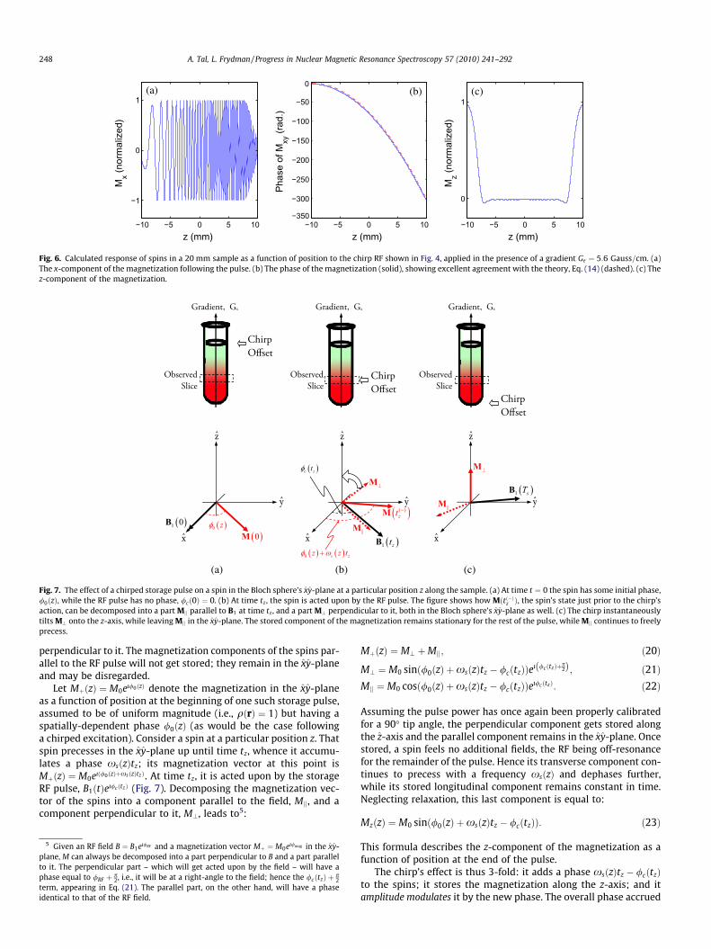
Fig. 6. Calculated response of spins in a 20 mm sample as a function of position to the chirp RF shown in Fig. 4, applied in the presence of a gradient Ge ¼ 5:6 Gauss=cm. (a)The x-component of the magnetization following the pulse. (b) The phase of the magnetization (solid), showing excellent agreement with the theory, Eq. (14) (dashed). (c) Thez-component of the magnetization.
Fig. 7. The effect of a chirped storage pulse on a spin in the Bloch sphere’s xy-plane at a particular position z along the sample. (a) At time t ¼ 0 the spin has some initial phase,/0ðzÞ, while the RF pulse has no phase, /cð0Þ ¼ 0. (b) At time tz , the spin is acted upon by the RF pulse. The figure shows how Mðtð�Þz Þ, the spin’s state just prior to the chirp’saction, can be decomposed into a part Mjj parallel to B1 at time tz , and a part M? perpendicular to it, both in the Bloch sphere’s xy-plane as well. (c) The chirp instantaneouslytilts M? onto the z-axis, while leaving Mjj in the xy-plane. The stored component of the magnetization remains stationary for the rest of the pulse, while Mjj continues to freelyprecess.
248 A. Tal, L. Frydman / Progress in Nuclear Magnetic Resonance Spectroscopy 57 (2010) 241–292
perpendicular to it. The magnetization components of the spins par-allel to the RF pulse will not get stored; they remain in the xy-planeand may be disregarded.
Let MþðzÞ ¼ M0eı/0ðzÞ denote the magnetization in the xy-planeas a function of position at the beginning of one such storage pulse,assumed to be of uniform magnitude (i.e., qðrÞ ¼ 1) but having aspatially-dependent phase /0ðzÞ (as would be the case followinga chirped excitation). Consider a spin at a particular position z. Thatspin precesses in the xy-plane up until time tz, whence it accumu-lates a phase xsðzÞtz; its magnetization vector at this point isMþðzÞ ¼ M0eıð/0ðzÞþxsðzÞtzÞ. At time tz, it is acted upon by the storageRF pulse, B1ðtÞeı/cðtzÞ (Fig. 7). Decomposing the magnetization vec-tor of the spins into a component parallel to the field, Mjj, and acomponent perpendicular to it, M?, leads to5:
5 Given an RF field B ¼ B1eı/RF and a magnetization vector Mþ ¼ M0eı/mag in the xy-plane, M can always be decomposed into a part perpendicular to B and a part parallelto it. The perpendicular part – which will get acted upon by the field – will have aphase equal to /RF þ p
2, i.e., it will be at a right-angle to the field; hence the /cðtzÞ þ p2
term, appearing in Eq. (21). The parallel part, on the other hand, will have a phaseidentical to that of the RF field.
MþðzÞ ¼ M? þMjj; ð20Þ
M? ¼ M0 sinð/0ðzÞ þxsðzÞtz � /cðtzÞÞeı /cðtzÞþp2ð Þ; ð21Þ
Mjj ¼ M0 cosð/0ðzÞ þxsðzÞtz � /cðtzÞÞeı/c ðtzÞ: ð22Þ
Assuming the pulse power has once again been properly calibratedfor a 90� tip angle, the perpendicular component gets stored alongthe z-axis and the parallel component remains in the xy-plane. Oncestored, a spin feels no additional fields, the RF being off-resonancefor the remainder of the pulse. Hence its transverse component con-tinues to precess with a frequency xsðzÞ and dephases further,while its stored longitudinal component remains constant in time.Neglecting relaxation, this last component is equal to:
MzðzÞ ¼ M0 sinð/0ðzÞ þxsðzÞtz � /cðtzÞÞ: ð23Þ
This formula describes the z-component of the magnetization as afunction of position at the end of the pulse.
The chirp’s effect is thus 3-fold: it adds a phase xsðzÞtz � /cðtzÞto the spins; it stores the magnetization along the z-axis; and itamplitude modulates it by the new phase. The overall phase accrued

A. Tal, L. Frydman / Progress in Nuclear Magnetic Resonance Spectroscopy 57 (2010) 241–292 249
can be calculated by substituting xs; tz, and /cðtÞ (Eqs. (19), (18)and (9)) explicitly:
xsðzÞtz�/cðtzÞ ¼ðcGsÞ2
2R
!z2þ �cGsðOi�X1Þ
R
� �zþ ðOi�X1Þ2
2R
!:
ð24Þ
The calibration of chirped storage pulses is identical to that ofexcitation pulses, as discussed in Section 2.2.1.
2.4. Chirped p-pulses
Chirped pulses can be used not only to excite and store spins,but also to invert or flip them in the xy-plane. Such RF sweeps be-long to the family of ‘‘adiabatic” pulses, known to preserve the rel-ative angle between the spin magnetization and the effectivemagnetic field in a suitable rotating frame. In particular, chirpedp-pulses are functionally similar to excitation and storage chirps(Eq. (8) and Fig. 4), but possess higher power levels so as to pro-duce a 180� flip angle.
The mechanism by which such a p flip is produced warrantsfurther discussion. Much like the p
2 chirp, a swept p chirp flips spins‘‘instantaneously” when its resonant frequency matches the pre-cession frequency of the spins. Unlike the p
2 chirp, a p chirp con-serves the relative angle h between the spins’ magnetization andthe effective B-field as it changes [25,26,23]. This is best under-stood in a frequency-modulated frame rotating about the z-axis atthe same rate as the RF field. In such a frame, the total magneticfield – which, in the rotating frame is of the form cBrotðtÞ ¼ðcB1ðtÞ cosð/cðtÞÞ; cB1ðtÞ sinð/cðtÞÞ;X1Þ – becomes6
cBFMðtÞ ¼ cB1ðtÞ;0;X1 þ OðtÞð Þ: ð25Þ
Note the additional OðtÞ ‘‘fictitious force” term added to the z-com-ponent, as a result of the non-uniform rotation of this frame of ref-erence. In this frequency-modulated (FM) frame, the RF fieldremains in the x–z plane, and its constant x-component implies thatthe field vector BFMðtÞ sweeps out a triangle. Assuming for simplic-ity that the chemical shift is significantly smaller than the chirpbandwidth, i.e., X1 DO, implies that, in this frame, BFM startsout and ends up being almost parallel to the z-axis, as illustratedin Fig. 8.
The adiabatic theorem [27] states that, when the RF field’sdirection varies more slowly than the precession frequency of thespins (imposed by BFM), the angle between the field and the spins isconserved.7 A direct consequence of the adiabatic theorem is thatthe angle h between the field and the spins is time-invariant. Of par-ticular relevance for the present discussion is a state where spinpackets are initially distributed in the xy-plane, represented by theshaded disc in Fig. 8. This plane rotates adiabatically along with theRF field in such a way as to conserve h. Fig. 9 plots the effect calcu-lated for such a swept p-pulse, applied in the presence of a linear z-gradient, on an ensemble of spins assumed to be initially along the zor the x axes of the Bloch sphere. In the former case, the typical fol-lowing of Mz and BFM is easily discernable.
From a standpoint of spatial encoding, it is relevant to computenot only the rotation but also the phase imparted by these chirpedp-pulses. This analysis of p-chirps is similar to that of the p
2-chirpsdiscussed earlier. Assuming a pulse having duration TðpÞ is appliedin the presence of a gradient GðpÞ, a spin with chemical shift X1 and
6 The chirp envelope, B1ðtÞ, will be assumed constant. Slightly smoothed B1
amplitude envelopes (e.g., Eq. (17)) will modulate the response, but not alter theconclusions derived herein.
7 This fact is used in the design of adiabatic inversion pulses, in which the RF fieldand spins start along parallel to the z axis, and – by slowly sweeping the field until itpoints along �z – one can ensure that the spin follow it, ending up pointing along the�z direction as well.
position z will have its off-resonance frequency given byxðpÞðzÞ ¼ X1 þ cGðpÞz. An RF endowed with a linear frequencysweep given by Eq. (10) will – once again, to a good approximation– flip the spin only when xc matches xðpÞ for that z. This will occurat a time tz such that xcðtzÞ ¼ xðpÞðzÞ. Solving explicitly for tz, Eq.(12) is recovered, with Ge swapped for GðpÞ. A spin with an initialphase /0 positioned at z will, therefore, precess freely until timetz and acquire a phase xðpÞtz. At this instant, the chirp will effec-tively flip this spin with respect to an axis colinear with the RFpulse at time tz. Assuming, as before, that /cðtÞ �
R t0 xcðt0Þdt0 will
be the phase of this RF at time t into the pulse, then /cðtzÞ is alsothe angle with the x-axis in the xy-plane, with respect to whichthe spin at z is p-flipped. As a result of this effect the phase ofthe spin will become �/0 þ 2/cðtzÞ �xðpÞðzÞtz, where /0 is the spinphase before applying the chirp. The magnetization vector willthen continue precessing with a frequency xðpÞðzÞ for the remain-ing duration of the pulse, TðpÞ � tz, and will hence acquire an addi-tional phase xðpÞðzÞðTðpÞ � tzÞ. The total phase of the magnetizationvector at the end of the pulse is therefore
/ðpÞðzÞ ¼ �/0ðzÞ þ 2/cðtzÞ � 2xðpÞðzÞtz þxðpÞðzÞTðpÞ: ð26Þ
This sequence of events is described pictorially in Fig. 10, with atime plots of the xy magnetization components for spins at differ-ent positions along the sample shown in Fig. 11. By substitutingthe explicit expressions for xðpÞ and tz into Eq. (26), this overall/ðpÞðzÞ phase can be explicitly calculated:
/ðpÞðzÞ ¼ �/0ðzÞ �cGðpÞ� �2
R
0B@1CAz2
þ 2cGðpÞðOi �X1ÞR
þ cGðpÞT ðpÞ !
z
þ T ðpÞX1 �ðOi �X1Þ2
R
!: ð27Þ
An important consideration in all this analysis is whether andwhen the RF chirp fulfills the adiabaticity condition. This can be ex-posed explicitly using Eq. (25) to compute the angle a between thefield in the frequency-modulated frame, BFM , and the x-axis. Usingstraightforward trigonometry :
aðtÞ ¼ arctanX1 � OðtÞ
cB1
�: ð28Þ
The magnitude of the derivative of this angle then measures therate of change of the field direction, and is given by:
daðtÞdt
¼ cB1R
ðOðtÞ þX1Þ2 þ ðcB1Þ2: ð29Þ
By differentiating and equating the result to zero, da=dt is found toreach its maximal value at
textremum ¼TðpÞ
2�X1
R� TðpÞ
2; ð30Þ
this value is8 jda=dtjmax ¼ R=cB1. On the other hand, the spin preces-sion frequency about BFMðtÞ is
xeff ðtÞ ¼ cBFMðtÞj j; ð31Þ
and is slowest when BFM is smallest, that is, at t ¼ textremum, when itsz-component is 0 and jcBFMj ¼ cB1 � xeff;min (see Fig. 12). The RFfield BFM will remain ‘‘adiabatic” as long as its rate of change is
8 This is geometrically sound, as the maximum occurs roughly halfway through thepulse, when the field’s z-component is 0 and its change is most pronounced (seeFig. 8b).

Fig. 8. Adiabatic RF p chirp, viewed in a frequency-modulated (FM) frame at: (a) the beginning of the chirp; (b) midway through the chirp; (c) at its conclusion. The shadeddisc represents the spins in the xy-plane at the beginning of the pulse. Due to the pulse’s adiabaticity, the angle between the disc and the field is kept constant throughout thepulse, effectively flipping the spins in the xy-plane.
−10 −5 0 5 100
1
z (mm)
|Mxy
| (no
rmal
ized
)
(a)
−10 −5 0 5 10−300
−250
−200
−150
−100
−50
0
z (mm)
Phas
e of
Mxy
(rad
.)
(b)
−10 −5 0 5 10−1
0
1
z (mm)M
z (nor
mal
ized
)
(c)
−10 −5 0 5 100
1
z (mm)
|Mxy
| (no
rmal
ized
)
(d)
−10 −5 0 5 10−100
−50
0
50
100
z (mm)
Phas
e of
Mxy
(rad
.)
(e)
−10 −5 0 5 10−1
0
1
z (mm)
Mz (n
orm
aliz
ed)
(f)
Fig. 9. Calculated response of spins in a 20 mm sample, as a function of position, to a p-chirp, applied in the presence of a gradient G ¼ 4:7 Gauss=cm. The spins wereassumed to start out either along the z-axis (top panels, a–c) with an initial magnetization vector M ¼ ð0;0;1Þ, or the x-axis (bottom panels, d–f), with an initial magnetizationvector M ¼ ð1;0;0Þ. (a and d) The absolute value of the magnetization’s projection on the xy-plane. (b and e) The phase induced by the chirp in the transverse plane. Note in(e) the agreement with between the simulated result (solid, blue) and the theoretical quadratic prediction, as given by Eq. (27) (red, dashed). (c and f) The z-component of themagnetization. (For interpretation of the references to color in this figure legend, the reader is referred to the web version of this article.)
250 A. Tal, L. Frydman / Progress in Nuclear Magnetic Resonance Spectroscopy 57 (2010) 241–292
slower than the spins’ precession about it; this is assured to holdthroughout the chirp if jda=dtjmax xeff;min, and furnishes the clas-sical condition:
cB1 �ffiffiffiRp
: ð32Þ
Further discussions on this can be found in [28].Due to their adiabatic nature, the calibration of p chirps is
somewhat different from that described for their p2 counterparts.
As shown in Eq. (32), the RF’s power in kHz must be larger thanffiffiRp
2p. In practice, it is found that setting cB1 to be at least 2.5 timeslarger than the power for an equivalent p
2 chirp (Eq. (15)),achieves an adequate performance. It must also be borne inmind that, in accordance with the analysis presented in Sec-
tion 2.4, the p chirp approximations break down for chemicalshifts comparable to the chirp’s bandwidth; this is evident inthe tails of the frequency responses plotted in Fig. 9. To ensurea constant response, the chirp’s bandwidth must be suitablyenlarged.
3. Single-scan ultrafast 2D NMR
3.1. Approaches to spatial encoding
Having introduced the spin evolutions imparted by differentchirped RF pulses and the action of gradients, the principles atthe heart of single-scan 2D NMR can now be outlined. This is

Fig. 10. Time evolution of a spin’s magnetization vector, M, situated at z during the application of a p-chirp. (a) Initially, at t ¼ 0;M is assumed already in the xy-plane withsome initial phase /0ðzÞ. (b) M precesses freely and accumulates a phase xðpÞtz until acted upon by the RF pulse. The figure shows M right prior to being flipped, Mxyðtð�Þz Þ(solid) and right after, MxyðtðþÞz Þ (dashed). Note that the axis around which the spin is flipped is colinear with the RF pulse at time tz , i.e., an axis in the xy-plane making anangle /cðtzÞ with the x-axis. Following the chirp action, the phase of M becomes �/0ðzÞ þ 2/cðtzÞ �xðpÞðzÞtz . (c) Following the p-flip, M continues precessing freely until theend of the pulse at time T ðpÞ , accumulating a additional phase xðpÞðTðpÞ � tzÞ. The total phase of the magnetization vector at the end of the pulse is, therefore,�/0ðzÞ þ 2/cðtzÞ � 2xðpÞðzÞtz þxðpÞðzÞTðpÞ.
A. Tal, L. Frydman / Progress in Nuclear Magnetic Resonance Spectroscopy 57 (2010) 241–292 251
spatial encoding; i.e., the physical partitioning of a sample intoan array of voxels possessing different evolution periods. Theobjective, we remind again, is the creation of a position-depen-dent t1 evolution time of the form t1ðzÞ ¼ Cz. This section focuseson achieving this goal by the three schemes detailed in Fig. 13;additional schemes are discussed in [29–32]. For simplicity, weshall assume in what follows that all chirps have symmetricalbandwidths (namely that the range of frequencies they exciteis centered about 0, or, equivalently, that Of ¼ �Oi ¼ DO
2 ), so thatthe bandwidth, DO, is set equal to cGeL, where L is the sample’sphysical size9
3.1.1. Indirect-domain encoding with phase modulation p2 � p� �
Consider an ensemble of spins in thermal equilibrium, actedupon by a p
2 excitation chirp with rate Rp2ð Þ, duration T
p2ð Þ and
bandwidth DOp2ð Þ, in the presence of a gradient G
p2ð Þ. At the end
of such a pulse, the spins will have been excited onto thexy-plane, and will have accrued the phase given by Eq. (14). Sucha phase contains a part linear in z times the chemical shift, whichis desirable; but also an unwanted quadratic phase, proportionalto z2. In order to remove the latter, a p-chirp is applied, withduration T ðpÞ, rate RðpÞ and initial bandwidth DOðpÞ. This secondpulse keeps the spins in the xy-plane, but inverts their phase[33] and increments it as detailed in Eq. (27). By choosing2GðpÞTðpÞ ¼ G
p2ð ÞT p
2ð Þ, the phase of the spins following the p chirpwill be:
/p2�pðzÞ ¼ � cGðpÞT
p2ð ÞDO
p2ð Þ
2DOðpÞ
" #zþ
c GðpÞ � Gp2ð Þ
� �T
p2ð Þ
2pDOðpÞ
24 35X1z
þ p2� T
p2ð ÞX1
2þ T
p2ð ÞX2
1
4pDOp2ð Þ� TðpÞX2
1
2pDOðpÞ
!: ð33Þ
9 To avoid the imperfections in the frequency response near the edges of thebandwidth, one can set L slightly larger than the sample’s physical size, in effectexciting a wider bandwidth. A factor of 1.2 strikes a good compromise betweenachieving an even response and avoid irradiating frequencies not present in thesample.
Eq. (33) has precisely the form sought after. It has no quadratic termin z; it has a constant term, which merely phases the peaks and canbe dealt with using post-processing; it has a part linear in z andindependent of the chemical shift, which – as will be shown in Sec-tion 3.2 – moves the spectrum along the indirect domain and can befixed using a gradient Gp prior to acquisition (cf. Fig. 13a10); and ithas a term linear in both z and X1, of the form t1ðzÞX1 with
t1ðzÞ ¼ �c G
p2ð Þ � GðpÞ
� �T
p2ð Þ
DOðpÞz ¼ T
p2ð Þ � 2T pð Þ
Lz: ð34Þ
3.1.2. Indirect-domain encoding with amplitude modulation p2 � p
2
� �An alternative method to the one presented above uses two suc-
cessive p2-chirps to excite and store the spins [34], as illustrated in
Fig. 13b. The purpose of using two chirped pulses in both schemesis the same: the removal of the quadratic phase terms, propor-tional to z2. The current approach, however, differs from the previ-ous one by amplitude modulating the magnetization: the initial p
2excitation chirp tips the spins onto the xy-plane with a quadraticphase given by Eq. (14). At the end of the second p
2 storage chirp,part of the magnetization is stored along the z-axis and part re-mains in the xy-plane and is dephased by a strong gradient Gd,ensuring that transverse components will not contribute to the ac-quired signal. Assuming both chirps have equal durations T
p2ð Þ and
sweep rates Rp2ð Þ, and that the gradients used are equal and oppo-
site in sign, GðexciteÞ ¼ �GðstoreÞ � Gp2ð Þ, then the form of the magneti-
zation stored along the z-axis following the second chirped pulse is(see Eq. (23)):
MzðzÞ ¼ M0 sin �2cGp2ð ÞT p
2ð ÞzDO
p2ð Þ
X1 þ Tp2ð ÞX1 �
p2
" #: ð35Þ
Denoting
t1ðzÞ ¼ �2cG
p2ð ÞT p
2ð Þ
DOp2ð Þ
z ¼ 2Tp2ð Þz
L� tmax
1
Lz; ð36Þ
10 A purge gradient can also be used between the pulses to achieve the same end.

0
1
(c)
|Mxy
| (a.
u.)
0
1
(b)
|Mxy
| (a.
u.)
50 Time (ms)
0
1
(a)
|Mxy
| (a.
u.)
Gradient
+6 mm
0 mm
-6 mm
Fig. 11. The simulated evolution of the xy-component of the magnetization, for spins at different slices throughout a 20 mm sample, during a chirped p-pulse. The pulse, 5 mslong, was applied in the presence of a gradient G ¼ 4:7 Gauss=cm. The spins have all started out along the x-axis, with an initial magnetization vector M ¼ ð1;0;0Þ. Timeevolution is plotted for the slices z ¼ �6 mm; z ¼ 0 mm and z ¼ 6 mm in (a), (b) and (c), respectively.
252 A. Tal, L. Frydman / Progress in Nuclear Magnetic Resonance Spectroscopy 57 (2010) 241–292
where tmax1 � 2T
p2ð Þ is the total encoding time, one sees that MzðzÞ
can be written as M0 sin½t1ðzÞX1 þ ðconst: termsÞ�.Following the action of the dephasing gradient Gd, a mixing se-
quence is applied while the spins are stored, and the ensemble isthen tipped back onto the xy-plane using a hard-pulse. The result-ing transverse magnetization is then MþðzÞ / sinðt1ðzÞX1þwðzÞ þ aÞ, which can be written as the sum of complexexponentials:
MþðzÞ /12i
eı t1ðzÞX1þT
p2ð ÞX1�p
2
� �þ 1
2ie�ı t1ðzÞX1þT
p2ð ÞX1�p
2
� �: ð37Þ
The application of a purge gradient Gp for a duration Tp, as shown inFig. 13b, adds an additional phase cGpzTp to both exponentials. Asdiscussed in Section 3.3.2, the effect of such a phase is to shift theindirect-domain spectra. Hence, although both signals in Eq. (37)will contribute to the FID, it is possible to shift one of them outsidethe spectral width while observing the other. A somewhat similareffect, although with opposite signs for the two terms in Eq. (37),
could be introduced by a gradient pulse Gp acting before the storagechirped pulse.
3.1.3. Indirect-domain constant-time encoding ðp� pÞA third approach to spatial encoding relies on exciting the spins
with a hard p2 pulse, followed by two chirped p-pulses with identi-
cal sweeps but reversed gradients [35] (Fig. 13c). Assuming thatthe spins have initially been excited onto the x-axis, the first pchirp imparts to them a phase /ðpÞðzÞ given by Eq. (27), with/0ðzÞ ¼ 0. Following a second p chirp, the phase of the spins atthe end of the sequence is:
/ðp�pÞðzÞ ¼ �4cGðpÞTðpÞX1zDO
: ð38Þ
This once again gives the desired form, with
t1ðzÞ ¼ �4cGðpÞTðpÞ
DO¼ 4TðpÞ
Lz � 2tmax
1
Lz; ð39Þ
where tmax1 ¼ 2TðpÞ is the total encoding time.
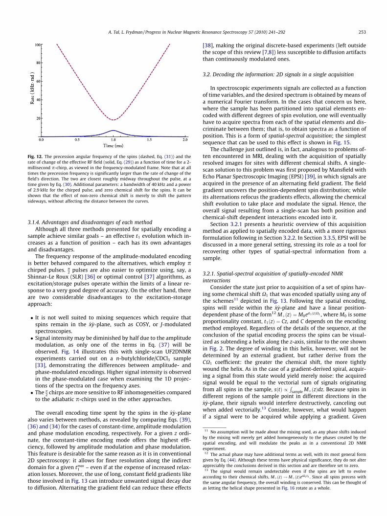
Fig. 12. The precession angular frequency of the spins (dashed, Eq. (31)) and therate of change of the effective RF field (solid, Eq. (29)) as a function of time for a 2-millisecond p-chirp, as viewed in the frequency-modulated frame. Note that at alltimes the precession frequency is significantly larger than the rate of change of thefield’s direction. The two are closest roughly midway throughout the pulse, at atime given by Eq. (30). Additional parameters: a bandwidth of 40 kHz and a powerof 2.9 kHz for the chirped pulse, and zero chemical shift for the spins. It can beshown that the effect of non-zero chemical shift is merely to shift the patternsideways, without affecting the distance between the curves.
11 No assumption will be made about the mixing used, as any phase shifts inducedby the mixing will merely get added homogeneously to the phases created by thespatial encoding, and will modulate the peaks as in a conventional 2D NMRexperiment.
12 The actual phase may have additional terms as well, with its most general formgiven by Eq. (44). Although these terms have physical significance, they do not alterappreciably the conclusions derived in this section and are therefore set to zero.
13 The signal would remain undetectable even if the spins are left to evolveaccording to their chemical shifts, MþðzÞ ! MþðzÞeıX2t2 . Since all spins precess withthe same angular frequency, the overall winding is conserved. This can be thought ofas letting the helical shape presented in Fig. 16 rotate as a whole.
A. Tal, L. Frydman / Progress in Nuclear Magnetic Resonance Spectroscopy 57 (2010) 241–292 253
3.1.4. Advantages and disadvantages of each methodAlthough all three methods presented for spatially encoding a
sample achieve similar goals – an effective t1 evolution which in-creases as a function of position – each has its own advantagesand disadvantages.
The frequency response of the amplitude-modulated encodingis better behaved compared to the alternatives, which employ pchirped pulses. p
2 pulses are also easier to optimize using, say, aShinnar-Le Roux (SLR) [36] or optimal control [37] algorithms, asexcitation/storage pulses operate within the limits of a linear re-sponse to a very good degree of accuracy. On the other hand, thereare two considerable disadvantages to the excitation-storageapproach:
� It is not well suited to mixing sequences which require thatspins remain in the xy-plane, such as COSY, or J-modulatedspectroscopies.� Signal intensity may be diminished by half due to the amplitude
modulation, as only one of the terms in Eq. (37) will beobserved. Fig. 14 illustrates this with single-scan UF2DNMRexperiments carried out on a n-butylchloride/CDCl3 sample[33], demonstrating the differences between amplitude- andphase-modulated encodings. Higher signal intensity is observedin the phase-modulated case when examining the 1D projec-tions of the spectra on the frequency axes.� The p
2 chirps are more sensitive to RF inhomogeneities comparedto the adiabatic p-chirps used in the other approaches.
The overall encoding time spent by the spins in the xy-planealso varies between methods, as revealed by comparing Eqs. (39),(36) and (34) for the cases of constant-time, amplitude modulationand phase modulation encoding, respectively. For a given z ordi-nate, the constant-time encoding mode offers the highest effi-ciency, followed by amplitude modulation and phase modulation.This feature is desirable for the same reason as it is in conventional2D spectroscopy: it allows for finer resolution along the indirectdomain for a given tmax
1 – even if at the expense of increased relax-ation losses. Moreover, the use of long, constant field gradients likethose involved in Fig. 13 can introduce unwanted signal decay dueto diffusion. Alternating the gradient field can reduce these effects
[38], making the original discrete-based experiments (left outsidethe scope of this review [7,8]) less susceptible to diffusion artifactsthan continuously modulated ones.
3.2. Decoding the information: 2D signals in a single acquisition
In spectroscopic experiments signals are collected as a functionof time variables, and the desired spectrum is obtained by means ofa numerical Fourier transform. In the cases that concern us here,where the sample has been partitioned into spatial elements en-coded with different degrees of spin evolution, one will eventuallyhave to acquire spectra from each of the spatial elements and dis-criminate between them; that is, to obtain spectra as a function ofposition. This is a form of spatial-spectral acquisition; the simplestsequence that can be used to this effect is shown in Fig. 15.
The challenge just outlined is, in fact, analogous to problems of-ten encountered in MRI, dealing with the acquisition of spatiallyresolved images for sites with different chemical shifts. A single-scan solution to this problem was first proposed by Mansfield withEcho Planar Spectroscopic Imaging (EPSI) [39], in which signals areacquired in the presence of an alternating field gradient. The fieldgradient uncovers the position-dependent spin distribution; whileits alternations refocus the gradients effects, allowing the chemicalshift evolution to take place and modulate the signal. Hence, theoverall signal resulting from a single-scan has both position andchemical-shift dependent interactions encoded into it.
Section 3.2.1 presents a heuristic overview of this acquisitionmethod as applied to spatially encoded data, with a more rigorousformulation following in Section 3.2.2. In Section 3.3.5, EPSI will bediscussed in a more general setting, stressing its role as a tool forrecovering other types of spatial-spectral information from asample.
3.2.1. Spatial-spectral acquisition of spatially-encoded NMRinteractions
Consider the state just prior to acquisition of a set of spins hav-ing some chemical shift X1 that was encoded spatially using any ofthe schemes11 depicted in Fig. 13. Following the spatial encoding,spins will reside within the xy-plane and have a linear position-dependent phase of the form12 MþðzÞ ¼ M0eıt1ðzÞX1 , where M0 is someproportionality constant, t1ðzÞ ¼ Cz, and C depends on the encodingmethod employed. Regardless of the details of the sequence, at theconclusion of the spatial encoding process the spins can be visual-ized as subtending a helix along the z-axis, similar to the one shownin Fig. 2. The degree of winding in this helix, however, will not bedetermined by an external gradient, but rather derive from theCX1 coefficient: the greater the chemical shift, the more tightlywound the helix. As in the case of a gradient-derived spiral, acquir-ing a signal from this state would yield merely noise: the acquiredsignal would be equal to the vectorial sum of signals originatingfrom all spins in the sample, sðtÞ /
Rsample MþðzÞdz. Because spins in
different regions of the sample point in different directions in thexy-plane, their signals would interfere destructively, canceling outwhen added vectorially.13 Consider, however, what would happenif a signal were to be acquired while applying a gradient. Given

Fig. 13. Different schemes discussed in this article for creating a different effective t1 evolution time in each slice. (a) Phase-modulated (PM) encoding. (b) Amplitude-modulated (AM) encoding. (c) Constant-time (CT) encoding. The arrows before each chirped pulse indicate the sign of DO, the bandwidth, which determines the directionalityof the sweep (from negative to positive frequencies or vice-versa).
254 A. Tal, L. Frydman / Progress in Nuclear Magnetic Resonance Spectroscopy 57 (2010) 241–292
enough time, this gradient could unwind the spins, and align thespin packets constructively so as to form an echo. Applying the gra-dient any longer would wind the aligned spins once again, causingthe signal to decay back into the noise.
This process is illustrated in Fig. 16 for two chemically inequiv-alent sites. Mathematically, it can be understood from the fact thatduring such an acquisition, the phases of the spins will evolve as/aðtÞ ¼ CX1zþ cGatz ¼ ðCX1 þ cGatÞz. It is seen that the spins alignwhen14 CX1 þ cGat ¼ 0; that is, when techo ¼ � C
cGaX1. The signal from
several chemical shifts is the superposition of signals from the indi-vidual chemical shifts, so a sample containing n different chemicalshifts, Xð1Þ1 ;Xð2Þ1 ; . . . ;XðnÞ1 prior to mixing will form n echoes, at loca-tions techo;j ¼ � C
cGaXðjÞ1 . Note that, since the position of an echo is pro-
portional to X1, the acquired echo pattern will in fact be proportional tothe spectrum along the indirect domain.
The gradient’s action just described is completely reversible:assuming no displacements, the spins can be rewound by following
14 In the event C is a positive quantity, Ga can be set to be negative, ensuring thattecho > 0 – that is, that the echo is indeed observed, provided one acquires for a timegreater than techo. For the purposes of the discussion in this section, it will be assumedthat Ga should be positive.
the positive gradient Ga with a negative one �Ga, having identicalmagnitude and duration. This has the effect of reversing whateverwinding was induced during the positive gradient lobe: the phaseadded by the positive gradient, cGaTaz, and the phase added by thenegative gradient, �cGaTaz, cancel out. Should a signal be acquiredin the presence of this negative gradient, the echoes will formagain, only in a reverse order, resulting in a pattern of echoeswhich is the mirror image of the one acquired in the presence ofthe positive gradient.
It would seem that – relaxation or diffusion notwithstanding –this process can be repeated indefinitely, leading to an identicaltrain of echoes and their mirror images by alternating the gradi-ent. This, however, would not take into account the fact that,alongside the gradient-induced winding, the spins precessaccording to their inherent t2-dependent chemical shifts. Hence,the echoes emanating from each chemical site will get addition-ally modulated by a term of the form eıX2t2 , representing its evo-lution by the action of the direct-domain chemical shift X2 (seeFig. 17a). This is the essence of the acquisition scheme: by acquir-ing spatially encoded data in the presence of a gradient, one canobserve the indirect-domain spectrum; by oscillating the gradientone can follow the eıX2t2 envelope modulating the indirect-domain

Fig. 14. Comparison between single-scan 2D TOCSY NMR spectra, acquired on a 500 MHz Varian iNova spectrometer, for an n-butylchloride/CDCl3 sample, utilizing theamplitude-modulated (a) and the phase-modulated (b) pulse sequences indicated on top. Also shown for the sake of a sensitivity comparison are the projections obtained ineach instance upon adding up all points along the indirect dimension (shown in absolute intensity mode). The effective tmax
1 encoding times are 40 and 45 ms in (A) and (B),respectively. Additional relevant parameters were gradient switching times of 10 ls, an L ¼ 1:8 cm sample length, and a 40 ms long DIPSI-2-type sequence applied in theabsence of gradients and over a 15 kHz bandwidth for the mixing. Also important to note are the cB1 settings used for the p
2 and p RF pulses: 200 and 1200 Hz, respectively.
Fig. 15. Echo Planar Spectroscopic Imaging (EPSI) sequence, used to acquire a different FID (or, equivalently, 1D spectrum) per position. In this sequence data are acquiredthroughout the action of an alternating gradient, shown here explicitly by the black dots.
15 This is a distinction worth stressing: the purpose of a mixing sequence is totransfer magnetization between coupled spins. Hence, spins having a chemical shift X1
will transfer their magnetization (and winding) to spins having some other chemicalshift X2; for instance, through couplings. Those spins would then precess duringacquisition with an off-resonance frequency given by X2. It is quite possible for X1 totransfer its magnetization to several spins; in this case, the overall chemical shiftevolution will reflect a linear superposition of the individual evolutions. Thisdiscussion will confine itself to a particular chemical shift, X2, along the direct domain.
A. Tal, L. Frydman / Progress in Nuclear Magnetic Resonance Spectroscopy 57 (2010) 241–292 255
echoes; that is, the evolution along the direct domain. Thus, theX1 � t2 plane can be covered, and a 2D spectrum acquired withina single-scan, by Fourier processing of such data versus t2
(Fig. 17b–e).
3.2.2. Mathematical formulation of the gradient-driven decodingDuring the process outlined in Fig. 17a, the acquisition phase of
a spin having a particular position z will evolve as a function of theacquisition time t2, as:
/aðz; t2Þ ¼ CX1zþ kðt2ÞzþX2t2: ð40Þ
Notice the distinction between X1, the indirect-domain chemicalshift prior to mixing, and X2, the chemical shift following the mix-ing.15 The variable kðt2Þ ¼ c
R t20 Gaðt0Þdt0, like the one introduced in
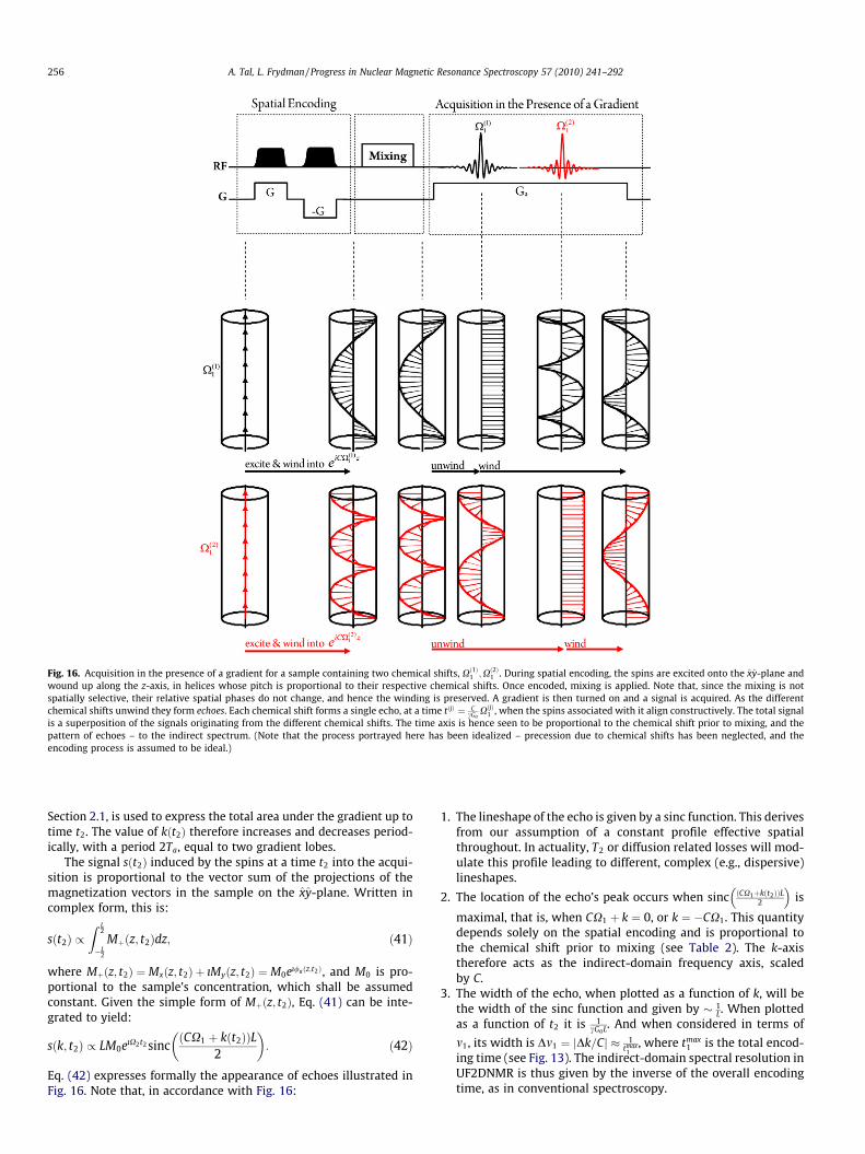
Fig. 16. Acquisition in the presence of a gradient for a sample containing two chemical shifts, Xð1Þ1 ;Xð2Þ1 . During spatial encoding, the spins are excited onto the xy-plane andwound up along the z-axis, in helices whose pitch is proportional to their respective chemical shifts. Once encoded, mixing is applied. Note that, since the mixing is notspatially selective, their relative spatial phases do not change, and hence the winding is preserved. A gradient is then turned on and a signal is acquired. As the differentchemical shifts unwind they form echoes. Each chemical shift forms a single echo, at a time tðjÞ ¼ C
cGaXðjÞ1 , when the spins associated with it align constructively. The total signal
is a superposition of the signals originating from the different chemical shifts. The time axis is hence seen to be proportional to the chemical shift prior to mixing, and thepattern of echoes – to the indirect spectrum. (Note that the process portrayed here has been idealized – precession due to chemical shifts has been neglected, and theencoding process is assumed to be ideal.)
256 A. Tal, L. Frydman / Progress in Nuclear Magnetic Resonance Spectroscopy 57 (2010) 241–292
Section 2.1, is used to express the total area under the gradient up totime t2. The value of kðt2Þ therefore increases and decreases period-ically, with a period 2Ta, equal to two gradient lobes.
The signal sðt2Þ induced by the spins at a time t2 into the acqui-sition is proportional to the vector sum of the projections of themagnetization vectors in the sample on the xy-plane. Written incomplex form, this is:
sðt2Þ /Z L
2
�L2
Mþðz; t2Þdz; ð41Þ
where Mþðz; t2Þ ¼ Mxðz; t2Þ þ ıMyðz; t2Þ ¼ M0eı/aðz;t2Þ, and M0 is pro-portional to the sample’s concentration, which shall be assumedconstant. Given the simple form of Mþðz; t2Þ, Eq. (41) can be inte-grated to yield:
sðk; t2Þ / LM0eıX2t2 sincðCX1 þ kðt2ÞÞL
2
� �: ð42Þ
Eq. (42) expresses formally the appearance of echoes illustrated inFig. 16. Note that, in accordance with Fig. 16:
1. The lineshape of the echo is given by a sinc function. This derivesfrom our assumption of a constant profile effective spatialthroughout. In actuality, T2 or diffusion related losses will mod-ulate this profile leading to different, complex (e.g., dispersive)lineshapes.
2. The location of the echo’s peak occurs when sinc ðCX1þkðt2ÞÞL2
� �is
maximal, that is, when CX1 þ k ¼ 0, or k ¼ �CX1. This quantitydepends solely on the spatial encoding and is proportional tothe chemical shift prior to mixing (see Table 2). The k-axistherefore acts as the indirect-domain frequency axis, scaledby C.
3. The width of the echo, when plotted as a function of k, will bethe width of the sinc function and given by � 1
L. When plottedas a function of t2 it is 1
cGaL. And when considered in terms of
m1, its width is Dm1 ¼ jDk=Cj � 1tmax1
, where tmax1 is the total encod-
ing time (see Fig. 13). The indirect-domain spectral resolution inUF2DNMR is thus given by the inverse of the overall encodingtime, as in conventional spectroscopy.

Fig. 17. Ultrafast 2D acquisition protocol and post-processing. (a) The signal in an UF2DNMR experiment is acquired in the presence of an alternating gradient. The echoesoriginating from the spins having a chemical shift X2 are modulated by eıX2 t2 . (b) The signal viewed in a 2D k� t2 space, where k ¼ kðt2Þ ¼ c
R t20 Gaðt0 Þdt0 . Note that kðt2Þ
represents the total area under the gradient and hence periodically increases and decreases as Ga flips sign. (c) To reach a final spectrum the positive (A and C) and negative (Band D) gradient data sets are separated. (d) Each data set is Fourier transformed over its t2 coordinate, with the dwell time being 2Ta . (e) The data sets can then be co-added toenhance the overall sensitivity.
A. Tal, L. Frydman / Progress in Nuclear Magnetic Resonance Spectroscopy 57 (2010) 241–292 257
4. The echo is modulated by an envelope eıX2t2 , implying thatsðk; t2Þ is in fact an indirect-domain frequency/direct-domaintime 2D interferogram. Thus, all it requires is a realignment ofits data points and a Fourier transform along t2 to yield thedesired 2D NMR spectrum. Indeed, the periodicity of kðtÞ dis-cussed earlier implies that kðt2 þ 2TaÞ ¼ kðt2Þ for all t2. In partic-ular, computing the phase difference D/a between two peaksseparated by 2Ta gives:
16 Althalso dep
D/a ¼ CX1zþ kðtecho þ 2TaÞ þX2ðtecho þ 2TaÞð Þ� CX1zþ kðtechoÞ þX2techoð Þ ¼ X22Ta: ð43Þ
Thus, the echo peaks are modulated solely by the chemical shiftevolution during acquisition, independent of the gradient, as illus-trated in Fig. 17a.
It is useful, for reasons that will become apparent shortly, tothink of k and t2 as independent variables.16 Each data point hasa particular value of ðk; t2Þ associated with it, and can therefore beviewed as being acquired in the k� t2 space along a trajectory de-fined by kðt2Þ, as shown in Fig. 17b. To implement the remainingFourier transform along t2, the data can then be separated andrearranged into two sets (Fig. 17c). These data sets contain points ac-quired during the positive and negative gradient lobes, respectively,and they are separable in the sense that their rows are proportional
ough k depends on t2 it can be viewed as an independent variable, since itends on GaðtÞ, which can be varied independently of t2.
to the spectrum along the indirect domain, while their columns – allof whose points are a 2Ta dwell-time apart – are modulated solely bythe post-mixing chemical shifts X2 (Eq. (43)). Fourier transformingover the columns (the t2 axis) at this point yields the direct-domainspectrum, and hence the desired 2D spectrum being sought(Fig. 17d). These two data sets, containing in principle identical 2Dspectral content, can be subsequently phased, re-registered (thiswould account for gradient and sampling non-idealities) and com-bined for the purpose of enhancing the sensitivity.
3.3. Practical considerations in ultrafast 2D NMR
Any two-dimensional spectrum involves a set of parameters,including the full widths at half height (FWHH) Dmi ði ¼ 1;2Þ ofthe peaks, the covered spectral widths SWi ði ¼ 1;2Þ, as well asthe signal-to-noise ratio (SNR), that define the overall quality andability of a method to discern the spectral information. The currentsection takes a closer look at these quantities in single-scan 2DNMR, and discusses additional issues such as the line shapes andthe use of purge gradients to shift the indirect-domain spectrum.In what follows, SWj will be used for describing the spectral widths,Dmj for the peaks’ FWHH, Ni ¼ SWi
Dmi; dtj for the dwell time and tmax
j forthe maximal acquisition time along the indirect ðj ¼ 1Þ and directðj ¼ 2Þ acquisition domains (t1 and t2, respectively).
3.3.1. Spectral characteristicsWe survey next explicit expressions for the spectral width and
resolution, SWj;Dmj, along the indirect ðj ¼ 1Þ and direct ðj ¼ 2Þ
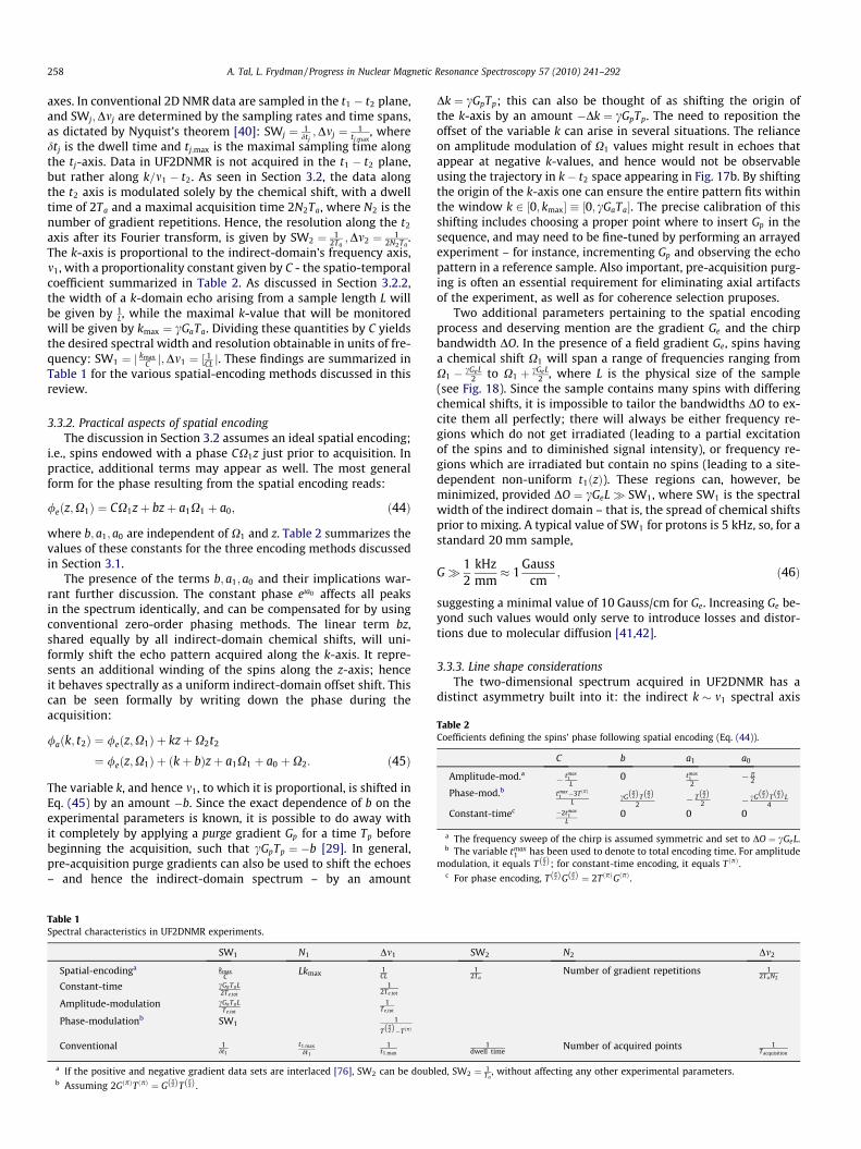
Table 2Coefficients defining the spins’ phase following spatial encoding (Eq. (44)).
C b a1 a0
Amplitude-mod.a � tmax1L
0 tmax12
� p2
Phase-mod.b tmax1 �3TðpÞ
LcG
p2ð ÞT p
2ð Þ2
� Tp2ð Þ
2 � cGp2ð ÞT p
2ð ÞL4
Constant-timec �2tmax1
L0 0 0
a The frequency sweep of the chirp is assumed symmetric and set to DO ¼ cGeL.b The variable tmax
1 has been used to denote to total encoding time. For amplitudemodulation, it equals T
p2ð Þ; for constant-time encoding, it equals TðpÞ .
c For phase encoding, Tp2ð ÞG
p2ð Þ ¼ 2TðpÞGðpÞ.
258 A. Tal, L. Frydman / Progress in Nuclear Magnetic Resonance Spectroscopy 57 (2010) 241–292
axes. In conventional 2D NMR data are sampled in the t1 � t2 plane,and SWj;Dmj are determined by the sampling rates and time spans,as dictated by Nyquist’s theorem [40]: SWj ¼ 1
dtj;Dmj ¼ 1
tj;max, where
dtj is the dwell time and tj;max is the maximal sampling time alongthe tj-axis. Data in UF2DNMR is not acquired in the t1 � t2 plane,but rather along k=m1 � t2. As seen in Section 3.2, the data alongthe t2 axis is modulated solely by the chemical shift, with a dwelltime of 2Ta and a maximal acquisition time 2N2Ta, where N2 is thenumber of gradient repetitions. Hence, the resolution along the t2
axis after its Fourier transform, is given by SW2 ¼ 12Ta;Dm2 ¼ 1
2N2Ta.
The k-axis is proportional to the indirect-domain’s frequency axis,m1, with a proportionality constant given by C - the spatio-temporalcoefficient summarized in Table 2. As discussed in Section 3.2.2,the width of a k-domain echo arising from a sample length L willbe given by 1
L, while the maximal k-value that will be monitoredwill be given by kmax ¼ cGaTa. Dividing these quantities by C yieldsthe desired spectral width and resolution obtainable in units of fre-quency: SW1 ¼ j kmax
C j;Dm1 ¼ ½ 1CL j. These findings are summarized inTable 1 for the various spatial-encoding methods discussed in thisreview.
3.3.2. Practical aspects of spatial encodingThe discussion in Section 3.2 assumes an ideal spatial encoding;
i.e., spins endowed with a phase CX1z just prior to acquisition. Inpractice, additional terms may appear as well. The most generalform for the phase resulting from the spatial encoding reads:
/eðz;X1Þ ¼ CX1zþ bzþ a1X1 þ a0; ð44Þ
where b; a1; a0 are independent of X1 and z. Table 2 summarizes thevalues of these constants for the three encoding methods discussedin Section 3.1.
The presence of the terms b; a1; a0 and their implications war-rant further discussion. The constant phase eıa0 affects all peaksin the spectrum identically, and can be compensated for by usingconventional zero-order phasing methods. The linear term bz,shared equally by all indirect-domain chemical shifts, will uni-formly shift the echo pattern acquired along the k-axis. It repre-sents an additional winding of the spins along the z-axis; henceit behaves spectrally as a uniform indirect-domain offset shift. Thiscan be seen formally by writing down the phase during theacquisition:
/aðk; t2Þ ¼ /eðz;X1Þ þ kzþX2t2
¼ /eðz;X1Þ þ ðkþ bÞzþ a1X1 þ a0 þX2: ð45Þ
The variable k, and hence m1, to which it is proportional, is shifted inEq. (45) by an amount �b. Since the exact dependence of b on theexperimental parameters is known, it is possible to do away withit completely by applying a purge gradient Gp for a time Tp beforebeginning the acquisition, such that cGpTp ¼ �b [29]. In general,pre-acquisition purge gradients can also be used to shift the echoes– and hence the indirect-domain spectrum – by an amount
Table 1Spectral characteristics in UF2DNMR experiments.
SW1 N1 Dm1
Spatial-encodinga kmaxC
Lkmax 1CL
Constant-time cGaTaL2Te;tot
12Te;tot
Amplitude-modulation cGaTaLTe;tot
1Te;tot
Phase-modulationb SW1 1
Tp2ð Þ�TðpÞ
Conventional 1dt1
t1;maxdt1
1t1;max
a If the positive and negative gradient data sets are interlaced [76], SW2 can be doubb Assuming 2GðpÞTðpÞ ¼ G
p2ð ÞT p
2ð Þ .
Dk ¼ cGpTp; this can also be thought of as shifting the origin ofthe k-axis by an amount �Dk ¼ cGpTp. The need to reposition theoffset of the variable k can arise in several situations. The relianceon amplitude modulation of X1 values might result in echoes thatappear at negative k-values, and hence would not be observableusing the trajectory in k� t2 space appearing in Fig. 17b. By shiftingthe origin of the k-axis one can ensure the entire pattern fits withinthe window k 2 ½0; kmax� � ½0; cGaTa�. The precise calibration of thisshifting includes choosing a proper point where to insert Gp in thesequence, and may need to be fine-tuned by performing an arrayedexperiment – for instance, incrementing Gp and observing the echopattern in a reference sample. Also important, pre-acquisition purg-ing is often an essential requirement for eliminating axial artifactsof the experiment, as well as for coherence selection pruposes.
Two additional parameters pertaining to the spatial encodingprocess and deserving mention are the gradient Ge and the chirpbandwidth DO. In the presence of a field gradient Ge, spins havinga chemical shift X1 will span a range of frequencies ranging fromX1 � cGeL
2 to X1 þ cGeL2 , where L is the physical size of the sample
(see Fig. 18). Since the sample contains many spins with differingchemical shifts, it is impossible to tailor the bandwidths DO to ex-cite them all perfectly; there will always be either frequency re-gions which do not get irradiated (leading to a partial excitationof the spins and to diminished signal intensity), or frequency re-gions which are irradiated but contain no spins (leading to a site-dependent non-uniform t1ðzÞ). These regions can, however, beminimized, provided DO ¼ cGeL� SW1, where SW1 is the spectralwidth of the indirect domain – that is, the spread of chemical shiftsprior to mixing. A typical value of SW1 for protons is 5 kHz, so, for astandard 20 mm sample,
G� 12
kHzmm
� 1Gauss
cm; ð46Þ
suggesting a minimal value of 10 Gauss/cm for Ge. Increasing Ge be-yond such values would only serve to introduce losses and distor-tions due to molecular diffusion [41,42].
3.3.3. Line shape considerationsThe two-dimensional spectrum acquired in UF2DNMR has a
distinct asymmetry built into it: the indirect k � m1 spectral axis
SW2 N2 Dm2
12Ta
Number of gradient repetitions 12TaN2
1dwell time
Number of acquired points 1Tacquisition
led, SW2 ¼ 1Ta
, without affecting any other experimental parameters.
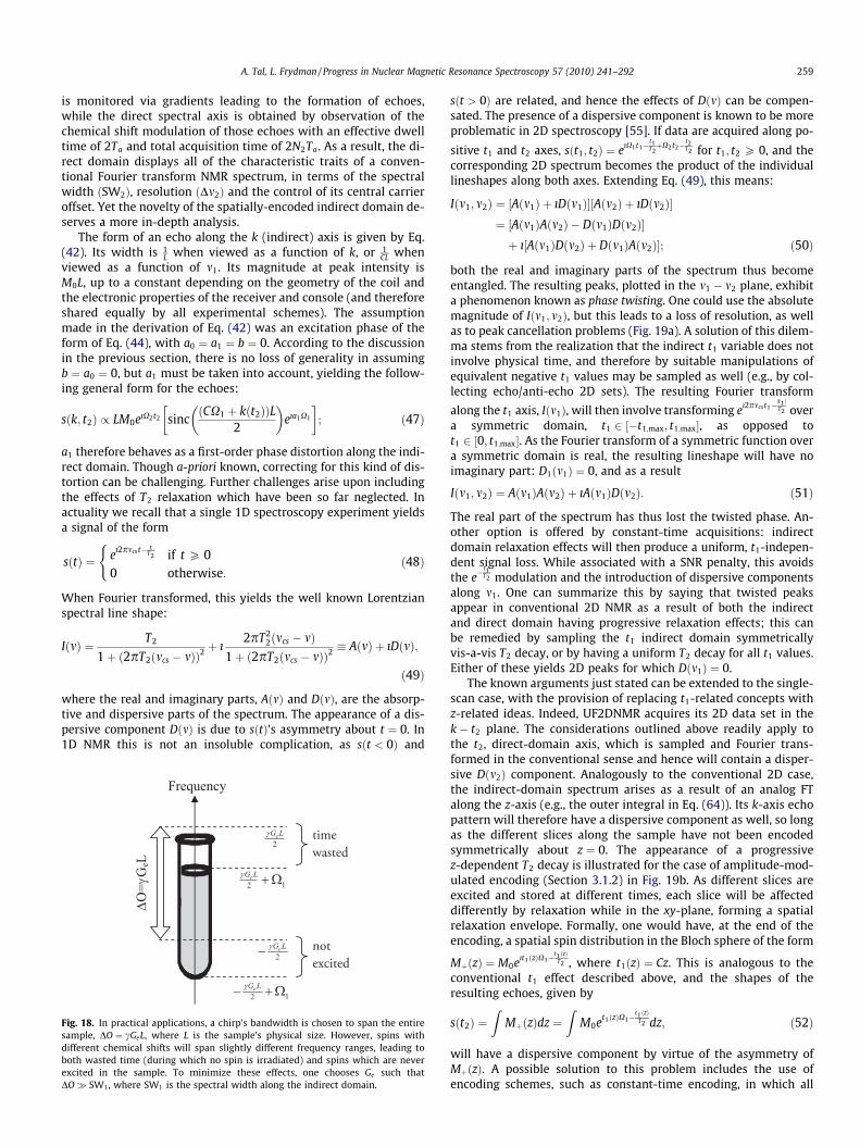
A. Tal, L. Frydman / Progress in Nuclear Magnetic Resonance Spectroscopy 57 (2010) 241–292 259
is monitored via gradients leading to the formation of echoes,while the direct spectral axis is obtained by observation of thechemical shift modulation of those echoes with an effective dwelltime of 2Ta and total acquisition time of 2N2Ta. As a result, the di-rect domain displays all of the characteristic traits of a conven-tional Fourier transform NMR spectrum, in terms of the spectralwidth ðSW2Þ, resolution ðDm2Þ and the control of its central carrieroffset. Yet the novelty of the spatially-encoded indirect domain de-serves a more in-depth analysis.
The form of an echo along the k (indirect) axis is given by Eq.(42). Its width is 1
L when viewed as a function of k, or 1CL when
viewed as a function of m1. Its magnitude at peak intensity isM0L, up to a constant depending on the geometry of the coil andthe electronic properties of the receiver and console (and thereforeshared equally by all experimental schemes). The assumptionmade in the derivation of Eq. (42) was an excitation phase of theform of Eq. (44), with a0 ¼ a1 ¼ b ¼ 0. According to the discussionin the previous section, there is no loss of generality in assumingb ¼ a0 ¼ 0, but a1 must be taken into account, yielding the follow-ing general form for the echoes:
sðk; t2Þ / LM0eıX2t2 sincðCX1 þ kðt2ÞÞL
2
� �eıa1X1
�; ð47Þ
a1 therefore behaves as a first-order phase distortion along the indi-rect domain. Though a-priori known, correcting for this kind of dis-tortion can be challenging. Further challenges arise upon includingthe effects of T2 relaxation which have been so far neglected. Inactuality we recall that a single 1D spectroscopy experiment yieldsa signal of the form
sðtÞ ¼ eı2pmcst� tT2 if t P 0
0 otherwise:
(ð48Þ
When Fourier transformed, this yields the well known Lorentzianspectral line shape:
IðmÞ ¼ T2
1þ ð2pT2ðmcs � mÞÞ2þ ı
2pT22ðmcs � mÞ
1þ ð2pT2ðmcs � mÞÞ2� AðmÞ þ ıDðmÞ;
ð49Þ
where the real and imaginary parts, AðmÞ and DðmÞ, are the absorp-tive and dispersive parts of the spectrum. The appearance of a dis-persive component DðmÞ is due to sðtÞ’s asymmetry about t ¼ 0. In1D NMR this is not an insoluble complication, as sðt < 0Þ and
Fig. 18. In practical applications, a chirp’s bandwidth is chosen to span the entiresample, DO ¼ cGeL, where L is the sample’s physical size. However, spins withdifferent chemical shifts will span slightly different frequency ranges, leading toboth wasted time (during which no spin is irradiated) and spins which are neverexcited in the sample. To minimize these effects, one chooses Ge such thatDO� SW1, where SW1 is the spectral width along the indirect domain.
sðt > 0Þ are related, and hence the effects of DðmÞ can be compen-sated. The presence of a dispersive component is known to be moreproblematic in 2D spectroscopy [55]. If data are acquired along po-
sitive t1 and t2 axes, sðt1; t2Þ ¼ eıX1t1�t1T2þX2t2�
t2T2 for t1; t2 P 0, and the
corresponding 2D spectrum becomes the product of the individuallineshapes along both axes. Extending Eq. (49), this means:
Iðm1; m2Þ ¼ Aðm1Þ þ ıDðm1Þ½ � Aðm2Þ þ ıDðm2Þ½ �¼ Aðm1ÞAðm2Þ � Dðm1ÞDðm2Þ½ �þ ı Aðm1ÞDðm2Þ þ Dðm1ÞAðm2Þ½ �; ð50Þ
both the real and imaginary parts of the spectrum thus becomeentangled. The resulting peaks, plotted in the m1 � m2 plane, exhibita phenomenon known as phase twisting. One could use the absolutemagnitude of Iðm1; m2Þ, but this leads to a loss of resolution, as wellas to peak cancellation problems (Fig. 19a). A solution of this dilem-ma stems from the realization that the indirect t1 variable does notinvolve physical time, and therefore by suitable manipulations ofequivalent negative t1 values may be sampled as well (e.g., by col-lecting echo/anti-echo 2D sets). The resulting Fourier transform
along the t1 axis, Iðm1Þ, will then involve transforming eı2pmcst1�jt1 jT2 over
a symmetric domain, t1 2 ½�t1;max; t1;max�, as opposed tot1 2 ½0; t1;max�. As the Fourier transform of a symmetric function overa symmetric domain is real, the resulting lineshape will have noimaginary part: D1ðm1Þ ¼ 0, and as a result
Iðm1; m2Þ ¼ Aðm1ÞAðm2Þ þ ıAðm1ÞDðm2Þ: ð51Þ
The real part of the spectrum has thus lost the twisted phase. An-other option is offered by constant-time acquisitions: indirectdomain relaxation effects will then produce a uniform, t1-indepen-dent signal loss. While associated with a SNR penalty, this avoidsthe e�
t1T2 modulation and the introduction of dispersive components
along m1. One can summarize this by saying that twisted peaksappear in conventional 2D NMR as a result of both the indirectand direct domain having progressive relaxation effects; this canbe remedied by sampling the t1 indirect domain symmetricallyvis-a-vis T2 decay, or by having a uniform T2 decay for all t1 values.Either of these yields 2D peaks for which Dðm1Þ ¼ 0.
The known arguments just stated can be extended to the single-scan case, with the provision of replacing t1-related concepts withz-related ideas. Indeed, UF2DNMR acquires its 2D data set in thek� t2 plane. The considerations outlined above readily apply tothe t2, direct-domain axis, which is sampled and Fourier trans-formed in the conventional sense and hence will contain a disper-sive Dðm2Þ component. Analogously to the conventional 2D case,the indirect-domain spectrum arises as a result of an analog FTalong the z-axis (e.g., the outer integral in Eq. (64)). Its k-axis echopattern will therefore have a dispersive component as well, so longas the different slices along the sample have not been encodedsymmetrically about z ¼ 0. The appearance of a progressivez-dependent T2 decay is illustrated for the case of amplitude-mod-ulated encoding (Section 3.1.2) in Fig. 19b. As different slices areexcited and stored at different times, each slice will be affecteddifferently by relaxation while in the xy-plane, forming a spatialrelaxation envelope. Formally, one would have, at the end of theencoding, a spatial spin distribution in the Bloch sphere of the form
MþðzÞ ¼ M0eıt1ðzÞX1�t1 ðzÞT2 , where t1ðzÞ ¼ Cz. This is analogous to the
conventional t1 effect described above, and the shapes of theresulting echoes, given by
sðt2Þ ¼Z
MþðzÞdz ¼Z
M0et1ðzÞX1�t1 ðzÞ
T2 dz; ð52Þ
will have a dispersive component by virtue of the asymmetry ofMþðzÞ. A possible solution to this problem includes the use ofencoding schemes, such as constant-time encoding, in which all

Fig. 19. (a) The absolute magnitude of data sampled in the t1 � t2 plane. Left: sampling just one quadrant of the t1 � t2 plane results in dispersive components along both axesand, hence, twisted phase. Right: the resolution is to sample the t1 axis symmetrically, eliminating the dispersive component along m1. (b) In UF2DNMR, amplitude-modulatedencoding leads to different slices residing in the xy-plane for different amounts of time, creating an asymmetrical spatial decay envelope, leading to a dispersive componentalong the acquisition’s k-axis. (c) One possible resolution is to use constant-time encoding, in which all slices spend the same amount of time in the xy-plane, and are equallyaffected by T2, leading to a symmetric spatial profile. (d) Another solution is to use the two phases arising in an amplitude-modulated encoding, and conduct one or twoexperiments that observe spatially the two terms in Eq. (37), which result in data sets along the k-axis with inverted dispersive components.
260 A. Tal, L. Frydman / Progress in Nuclear Magnetic Resonance Spectroscopy 57 (2010) 241–292
slices remain in the xy-plane for the same amount of time (this isillustrated in Fig. 19c). Another option is shown in Fig. 19d; it relieson the fact that, when the spins are stored, two spatial mirror-images of the spin distribution – akin to the echo/anti-echo modu-lations mentioned earlier – are retained. These can be distinguishedduring the acquisition (Eq. (37)). One of the terms can be observedby monitoring the positive k-values, while the other can be ob-served by monitoring the negative k-values. This can be achievedin two separate experiments with inverted gradient patterns [22],as shown in Fig. 19d; alternatively, they can be monitored in a sin-gle scan, at the expense of shifting the whole pattern and doublingthe kmax range. Regardless of the route, each resulting data set willhave dispersive components along the k-axis, equal in magnitudebut opposite in sign. Adding them up ensures the indirect-domainechoes are purely absorptive – mimicking the conventional 2D case.
In addition, options that find no direct counterpart in conventional2D NMR may arise in the spatially-encoded experiments. These in-clude, for example, the use of symmetric encoding schemes, such asthose discussed in [30].
In addition to these encoding-related phase distortions and cor-rections, the presence of the X2t2 phase in Eq. (49) is a general fea-ture of the indirect-domain acquisition. As data is acquired along askewed trajectory which is not parallel to the k-axis (see Fig. 17b),time-delays and first-order phase distortions will be present. Butno special considerations related to the lineshapes along m2 willarise.
3.3.4. Signal to noiseSignal-to-noise ratio (SNR) is a key practical aspect when con-
sidering the implementation of a UF2DNMR experiment. Indeed,
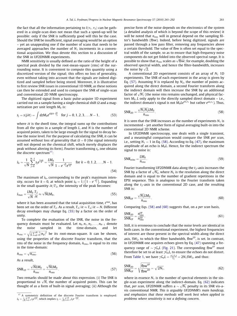
A. Tal, L. Frydman / Progress in Nuclear Magnetic Resonance Spectroscopy 57 (2010) 241–292 261
the fact that all the information pertaining to Iðm1; m2Þ can be gath-ered in a single-scan does not mean that such a speed-up will bepossible: only if the SNR is sufficiently good will this be the case.Should the SNR be insufficient, signal averaging would be an option– yet an unappealing one if the number of scans that needs to beaveraged approaches the number of N1 increments in a conven-tional acquisition. We thus devote this section to a discussion ofthe SNR in UF2DNMR experiments.
NMR sensitivity is usually defined as the ratio of the height of aspectral peak divided by the root-mean-square (rms) of the sur-rounding noise. It is convenient to compute this quantity using adiscretized version of the signal; this offers no loss of generality,even without taking into account that the signals are indeed digi-tized and sampled before being stored. Moreover, it is illustrativeto first review SNR issues in conventional 1D NMR, as these notionscan then be extended and used to compare the SNR of single-scanand conventional 2D NMR spectroscopy.
The digitized signal from a basic pulse-acquire 1D experimentcarried out on a sample having a single chemical shift X and a mag-netization per unit length M0 is:
sj ¼ sðjdtÞ ¼Z
dzM0eıXjdt�jdtT2 for j ¼ 0;1;2;3; . . . N � 1; ð53Þ
where dt is the dwell time, the integral sums up the contributionsfrom all the spins in a sample of length L, and N is the number ofacquired points, taken to be large enough for the signal to decay be-low the noise level. For the purpose of calculating the SNR, it can beassumed without loss of generality that X ¼ 0 (the signal intensitywill not depend on the chemical shift, which merely displaces thepeak without altering its form). Fourier transforming sj, one obtainsthe discrete spectrum17:
sk ¼1ffiffiffiffiNp
XN�1
j¼0
sje2pıjk
N ¼ LM0ffiffiffiffiNp 1
1� e�dtT2 e
2pıkN
for k ¼ 0;1;2; . . . ;N� 1:
ð54Þ
The maximum of sk, corresponding to the peak’s maximum inten-sity, occurs for k ¼ 0, at which point s0 ¼ 1= 1� e�
dtT2
� �. Expanding
in the small quantity dt=T2, the intensity of the peak becomes:
smax ¼LM0ffiffiffiffi
Np T2
dt�
ffiffiffiffiNp
LM0; ð55Þ
where it has been assumed that the total acquisition time, tmax, hasbeen set on the order of T2. As a result, T2=dt � Ta=dt ¼ N. Differentdecay envelopes may change Eq. (55) by a factor on the order ofunity.
To complete the evaluation of the SNR, the noise in the fre-quency domain must be evaluated. Let n0; n1; n2; . . . ;nN�1 denotethe noise sampled in the time-domain, and let
nrms ¼ffiffiffiffiffiffiffiffiffiffiffiffiffiffiffiffiffiffiffiffiffiffiffiffiffi1N
PN�1p¼0 jnpj2
qbe its root-mean-square. It can be shown,
using the properties of the discrete Fourier transform, that therms of the noise in the frequency domain, nrms, is equal to its rmsin the time-domain:
nrms ¼ffiffiffiffiffiffiffiffiffinrmsp
: ð56Þ
As a result,
SNR1D ¼ffiffiffiffiNp
LM0
nrms¼
ffiffiffiffiNp
LM0
nrms: ð57Þ
Two remarks should be made about this expression. (i) The SNR isproportional to
ffiffiffiffiNp
, the number of acquired points. This can bethought of as a form of built-in signal averaging; (ii) Although the
17 A symmetric definition of the discrete Fourier transform is employed:sk ¼ 1ffiffiffi
NpPN
j¼1sje2pıjk
N , which implies sj ¼ 1ffiffiffiNpPN
k¼1 sje�2pıjk
N .
precise form of the noise depends on the electronics of the system(a detailed analysis of which is beyond the scope of this review) itwill be noted that nrms will in general depend on the sampling fil-ter’s bandwidth (fbw). Indeed, before being digitized, signals arepassed through a low pass filter, removing any frequencies abovea certain threshold. The value of fbw is often set equal to the spec-tral width of the sample, so as to ensure that high-frequency noisecomponents do not get folded into the observed spectral range. It ispossible to show that nrms scales as
ffiffiffiffiffiffiffiffiffifbwp
; for example, doubling theobserved spectral width, and hence the filter-bandwidth, increasesthe noise by
ffiffiffi2p
.A conventional 2D experiment consists of an array of N1 1D
experiments. The SNR of each experiment in the array is given byEq. (57). Assuming N is replaced by N2, the number of points ac-quired along the direct domain, a second Fourier transform alongthe indirect domain will then increase the SNR by an additionalfactor of
ffiffiffiffiffiffiN1p
(the noise rms remains unchanged, and physical fac-tors M0; L only apply to the directly sampled direct domain – i.e.,the indirect domain’s signal is not M0LeıX1t1 but rather eıX1t1 ). Thus,
SNR2D ¼ffiffiffiffiffiffiffiffiffiffiffiffiN1N2p
LM0
nrms: ð58Þ
It is seen that the SNR increases as the number of experiments N1 isincremented – yet another form of signal averaging built-in into theconventional 2D NMR scheme.
In UF2DNMR spectroscopy, one deals with a single transient,and a meaningful comparison would compare the SNR per scan,i.e., setting N1 ¼ 1 in Eq. (58). According to Eq. (47), the maximumamplitude of an echo is M0L. Hence, for the indirect spectrum thesignal to noise is:
SNRecho ¼LM0
nrms: ð59Þ
Fourier transforming UF2DNMR data along the t2-axis increases theSNR by a factor of
ffiffiffiffiffiffiN2p
, where N2 is the resolution along the directdomain and is equal to the number of gradient repetitions in theEPSI sequence. This is analogous to the Fourier transform takenalong the t2-axis in the conventional 2D case, and the resultingSNR is:
SNRUF ¼ffiffiffiffiffiffiN2p
LM0
nrms: ð60Þ
Comparing Eqs. (58) and (60) suggests that, on a per scan basis,
SNR2D
SNRUF¼ nUF
rms
n2Drms
: ð61Þ
Still, it is erroneous to conclude that the noise levels are identical inboth cases. In the conventional experiment, the highest frequenciesof interest are those present in the spectral width along the direct
axis, SW2, to which the filter bandwidth, fbw2D, is set. In contrast,in UF2DNMR one acquires echoes given by Eq. (47) spanning a fre-
quency range of � cGaL (Fig. 21). The corresponding fbwUF musttherefore be set to at least cGaL, to ensure the echoes do not distort.From Table 1, we have cGaL ¼ cGaTaL
Ta¼ 2N1SW2, and thus:
SNR2D
SNRUF¼
ffiffiffiffiffiffiffiffiffiffiffiffiffifbwUF
fbw2D
s¼
ffiffiffiffiffiffiffiffiffi2N1
p: ð62Þ
where in essence N1 is the number of spectral elements in the sin-gle-scan experiment along the indirect-domain. Eq. (62) indicatesthat, per scan, UF2DNMR suffers a �
ffiffiffiffiffiffiN1p
penalty in its SNR vis-a-vis conventional NMR. This is arguably UF2DNMR’s main handicap,and emphasizes that these methods will work best when applied toproblems where sensitivity is not a defining concern.

Fig. 20. A schematic view of EPSI (note the axes have been tilted by 90� to facilitate the display of information). Once the acquired data has been arranged in a matrix (a), itcan be Fourier transformed about the k-axis to yield the FID from each slice (b). A second Fourier transform recovers the spectrum from each slice (c), and a third – the 2Dspectrum. Alternatively, a single Fourier transform over the t2 axis can be used to obtain the 2D spectrum directly (d).
Table 3Single-scan spatial-spectral acquisition: parameter relations.
To set . . . Set . . . to
SW2 The direct domain’s spectral width Ta The duration of the acquisition gradient’s lobe 12SW2
Dm2 The spectral resolution along the direct domain N2 The number of oscillations of the acquisition gradient 12TaDm2
SW1 The indirect domain’s spectral width Ga The acquisition gradient CSW1cTa
Dm1 The spectral resolution along the indirect domain t1max ¼ CL The effective encoding time (see Eqs. (34), (39), (36)) 1
Dm1
262 A. Tal, L. Frydman / Progress in Nuclear Magnetic Resonance Spectroscopy 57 (2010) 241–292
3.3.5. A formal view of EPSIWe have previously emphasized the use of oscillating acquisi-
tion gradients to acquire spatial-spectral information indepen-dently and simultaneously from different slices in the sample. Itis interesting to reformulate this acquisition block at an even morefundamental level than that presented in the previous sections;one which highlights its general applicability, in agreement withthe parallelization principle laid out at the beginning of this work.
Spins precessing in the transverse plane with a chemical shiftX2 and position z before commencing acquisition will, when sub-jected to the EPSI module in Fig. 15, give rise to a signal of theform:
sðk; t2Þ / eıðkðt2ÞzþX2t2Þ: ð63Þ
In order to describe a spatially-encoded sample, a generic distribu-tion in the xy-plane as a function of position and chemical shift,Iðz;X2Þ, must be taken into account. Iðz;X2Þ is proportional toMþðz;X2Þ, and so:
sensembleðk; t2Þ /Z
dzZ
dX2Mþðz;X2Þssingleðk; t2Þ
¼Z
dzZ
dX2Mþðz;X2Þeıkðt2ÞzeıX2t2 : ð64Þ
The signal, acquired in k� t2 space, is seen to be the Fourier-conju-gate of Mþðz;X2Þ; that is, Fourier transforming the signal sðk; t2Þalong its two variables will yield Mþðz;X2Þ. In actuality,sensembleðk; t2Þ is a discrete data set sampled at only specific pointsin the k� t2 plane, and as such it is subject to all the constraintsencountered when sampling a function. Furthermore, to avoidnon-regular sampling intervals, one can choose just those points ac-quired during the positive (or negative) gradient lobes, as wasshown in Fig. 17c. It follows from this that Mþðz0;X2Þ, for a fixedz0, represents the spectral distribution of spins in the slice whoseposition is z0. Carrying out a Fourier transform over X2 would thennaturally deliver the free induction decay for each z0 slice. This rea-soning is illustrated in the bottom panel of Fig. 20.
This general understanding of EPSI can also be used to deducewhy a single Fourier transform over the t2 variable is needed to re-cover a 2D spectrum in a UF2DNMR experiment. In conventionalspectroscopy, one executes several experiments, varying the delayalong the indirect t1 domain between each experiment; data isthen acquired along the direct t2 axis. Consequently, one needsto Fourier transform the resulting 2D data set along both axes, t1
and t2, to recover the 2D NMR spectrum. UF2DNMR works byparallelizing this notion, replacing the t1 domain by the z-axis.One can, by Fourier transforming the EPSI-acquired data over the

A. Tal, L. Frydman / Progress in Nuclear Magnetic Resonance Spectroscopy 57 (2010) 241–292 263
k variable, recover the FID of each experiment. This data set, in thez� t2 plane, is analogous to the data set conventionally acquired inthe t1 � t2 plane (Fig. 20b). It remains to Fourier transform this setagainst its two variables – z and t2 – to recover the 2D spectrum, asshown in Fig. 20d. This is equivalent to a single Fourier transforma-tion of sðk; t2Þ along the original t2 axis.
It is clear from the above discussion that the z� m2 plane is Fou-rier paired to the k� t2 plane, and as such, the range and resolutionviewable along the z; m2 axes is determined by the familiar Nyquistsampling relations. Still, as already mentioned, a distinction shouldbe drawn between the direct m2 domain, whose resolution dependssolely on the acquisition parameters Ta and N2, and an indirect m1
domain, whose resolution depends on the particular form of spatialencoding used during t1. Indeed, in ultrafast 2D NMR, where spinsare assigned a z-dependent t1 evolution, the particular form oft1 ¼ t1ðzÞ ¼ Cz will in turn define the k=m1 characteristics for eachencoding scheme (Fig. 13). Given C and the sample size L, theEPSI-described Nyquist sampling relations can thus be used tocompute the desired spectral characteristics as a function of theexperimental parameters. These results are summarized for conve-nience in Table 3.
3.3.6. ExamplesWith the theory underlying UF2DNMR outlined, this section
summarizes illustrative examples of spectra acquired using it.Fig. 22 demonstrates the viability of UF2DNMR on an 15N ubiquitinsample, comparing the resulting HSQC spectrum to one acquiredusing conventional 2D spectroscopy. It is seen that all essential fea-tures are retained in the single-scan version. As discussed in Sec-tion 3.3.3, phasing issues arise in UF2DNMR; for this reason, theabsolute magnitude of ultrafast spectra (instead of the real part)is usually used in those biomolecular applications. This leads to im-paired resolution along both axes by a factor of
ffiffiffi3p
. Still, Fig. 23demonstrates the ability of UF2DNMR to acquire spectra spacedat under a second, and utilize them to monitor a chemical processin real-time [43].
Fig. 24 shows how, by suitably altering the spatial encodingprotocol, various interactions can be suppressed and others al-lowed to evolve along the indirect domain [33]; specifically, thechemical shift evolution during encoding was refocused, whilethe J-coupling was allowed to evolve. This was achieved byphase-modulating the spins (see Section 3.1.2), equating the gradi-ents of both chirps while applying the p
2 pulse for twice as long asthe p-chirp. The resulting spatio-temporal coefficient C then be-comes null, voiding any chemical shift evolution along that axis,
Fig. 21. Filter bandwidth settings in conventional 2
while allowing for the J-coupling – unaffected by the p-pulse –to continue evolving.
Recent advances have also been made in applying UF2DNMR inconjunction with modern hyperpolarization methods [44,45]. Thesignal from the hyperpolarized nuclei, while large, decays rapidlywith a time constant T1, the magnitude of which is governed byspin-lattice relaxation and is on the order of a second. Since hyper-polarizing a sample may take hours, a full 2D spectrum may takedays to complete. The single-scan, sub-second nature of UF2DNMRbecomes particularly appealing in making the best use of this en-hanced signal. Several results are displayed in Fig. 25.
4. Spatial-spectral single-scan spectroscopy
The parallelization lying at the heart of UF2DNMR is made pos-sible by the use of chirped RF pulses, that excite spins onto thetransverse plane and endow them with a phase /ðz; mÞ ¼ Cmz. Suchmanipulation can be viewed as part of a larger superset of spatial-spectral pulses, which allow one to excite an arbitrary phase pat-tern in a position-frequency ðz� mÞ 2D space [46,47]. This sectiondiscusses how, by generalizing these reasonings (Fig. 26), the con-cept of parallelization can be extended to paradigms other than thesingle-scan UF2DNMR experiments just described. We begin thisdiscussion on extending the UF2DNMR paradigm by focusing onHadamard spectroscopy [48–52].
4.1. Conventional Hadamard spectroscopy: a review
In a standard 2D NMR experiment, one applies a mixing se-quence which transfers magnetization between sites based on par-ticular interactions that exist between them (Fig. 27a). Since manyfrequencies are present in the sample prior to mixing, the basicexperiment must be repeated for many t1 values: at leastN1 ¼ SW1=Dm1, to properly resolve all sites over a bandwidthSW1 with a minimal resolution Dm1. These experimental resultsare then arranged in a 2D matrix and Fourier transformed overboth axes, yielding a 2D spectrum in the m1; m2 domain.
As N1 will be given by local spectral characteristics – e.g., theclosest two peaks defining Dm1 and the farthest SW1, regardless ofwhere the remaining sites appear – one can envision a simplealternative to this completely general scheme: instead of excitingall chemical sites simultaneously and monitoring their time-do-main evolution, one could use a selective soft pulse to excite eachparticular chemical site, ma, as depicted in Fig. 27b. This would en-tail knowledge of the 1D spectrum prior to the 2D experiment, as
D versus single-scan ultrafast spectroscopies.

15N
[pp
m]
7.5 8 8.5 9 9.5 7.5 8 8.5 9 9.5
110
120
130
110
120
130
15N-Ubiquitin @ 2.3mM dissolved in 90%/10% H2O/D2O
Single-scan 2D HSQC -Cryoprobe
Conventional 2D (2048 scans) -RT probe
1H [ppm] 1H [ppm]
Fig. 22. A comparison between UF2DNMR and conventional 2D HSQC NMR spectra recorded at 18.8 T on a 3.25 mM 15N-enriched ubiquitin sample dissolved in 90/10%H2O=D2O (courtesy of Dr. Maayan Gal, Weizmann Institute).
18 Signal-averaging N experiments increases the signal-to-noise ratio by a factor offfiffiffiffiNp
[55].
264 A. Tal, L. Frydman / Progress in Nuclear Magnetic Resonance Spectroscopy 57 (2010) 241–292
one would have to know which frequency to irradiate. But sincethis scheme allows one to investigate only those lines of the 2Dspectrum that are of interest, one could dramatically reduce thenumber of experiments required for cases where both large band-widths and high spectral resolutions are needed, thus speeding upthe 2D acquisition. Indeed, in these selective-excitation experi-ments the t2 domain would include only frequencies originatingfrom ma prior to mixing. Fourier transforming this data wouldyield the m1 ¼ ma line from the full 2D spectrum. Each selective-excitation experiment then yields a particular m1 line of the full2D spectrum. This approach liberates one from the need to dis-cretely sample the t1 axis with a fine enough resolution: the res-olution along the m1 axis will be determined only by the width ofthe soft excitation pulse, which is inversely proportional to itsduration.
The above scheme suffers from a signal-to-noise penalty, in thesense that in each iteration only a single peak is excited. Contrastthis with conventional 2D spectroscopy, in which all peaks are ex-cited simultaneously. It is possible to find a solution to this draw-back [50], by exciting all peaks of interest simultaneously but withdifferent phases. This approach relies on a mathematical constructnamed Hadamard matrices [53] – hence the method, illustrated inFig. 27c, is referred to as 2D Hadamard NMR.
A Hadamard matrix H of order N is an N N construct thatsatisfies HHT ¼ NI, where I is the identity matrix. The HadamardConjecture [54] states that Hadamard matrices of order 4k existfor all positive integers k. Hadamard matrices of orders 2 and 4are:
H2 ¼1 11 �1
� �; H4 ¼
1 1 1 11 �1 1 �11 1 �1 �11 �1 �1 1
0BBB@1CCCA; ð65Þ
2D Hadamard spectroscopy’s approach is best illustrated via anexample. Suppose there are four frequencies of interest,ma; mb; mc; md, along the m1 axis. Four experiments are then carriedout; in the kth experiment, all four peaks are excited, each peakwith a phase of either 0 or p, in a pattern that corresponds to thekth row in the Hadamard matrix (Fig. 28a). The resulting four FIDsare then subtracted and added from each other in a pattern thatonce again follows the rows of the Hadamard matrix (Fig. 28b).The output of this is four 1D data sets, with the kth data set equiv-alent to the FID collected from an experiment in which a single fre-quency mk has been selectively excited, but with a
ffiffiffi4p
increase insignal to noise. This increase stems from the four experiments,which were added in such a way that one peak gets constructively
boosted, while all other peaks add destructively to zero.18 As signalaveraging four t1 increments could also give this sensitivity improve-ment, the multiplex advantage has been reinstated.
4.1.1. Complex Hadamard matricesAlthough Hadamard matrices exist only for orders N ¼ 2 and
N ¼ 4k where k is an integer, it is possible to extend the ideas dis-cussed in this section to any integer N by considering complex
Hadamard matrices [56], which are defined by HðcÞp;q ¼ e2pıðp�1Þðq�1Þ
N ;
p; q ¼ 1;2; . . . ;N. Like the real Hadamard matrices in Eq. (65), thesesatisfy HðcÞðHðcÞÞy ¼ NI, which is the essential characteristic neededby Hadamard spectroscopy. The complex Hadamard matrices oforders 2, 3 and 4 are:
HðcÞ2 ¼1 11 �1
� �; HðcÞ3 ¼
1 1 11 e
2pı3 e�
2pı3
1 e�2pı
3 e2pı3
0B@1CA; HðcÞ4 ¼
1 1 1 11 ı �1 �ı
1 �1 1 �11 �ı �1 ı
0BBB@1CCCA:ð66Þ
It is seen that, even for N ¼ 4, the real and complex Hadamardmatrices differ. When translated into NMR terms (for the N ¼ 4case), this means that, while the first experiment would excite allfour peaks with zero phase, the second would excite them withphases equal to 0; p2 ;p;
3p2 , respectively. Contrast this with an equiv-
alent experiment using real Hadamard matrices, for which the pulsephases for each peak would be set to 0;p;0;p. Despite these differ-ences, the arguments above can be repeated using complex Hadam-ard matrices, resulting in the same increase in signal to noise. In thiscase, the spectra must be added using the same phase coefficientsused to excite them–effectively, a sort of discrete Fourier transform.
Note that, while real Hadamard matrices require the selectiveexcitation to be real – that is to place the excited spins either alongx or �x in the Bloch sphere – their complex analogs require thespins to be evenly distributed in the xy plane of the Bloch sphere,a condition which may be more difficult to achieve experimentallyand to post-process.
4.2. Single-scan Hadamard spectroscopy
Parallelizing 2D Hadamard spectroscopy requires a sequencewhich will simultaneously excite all spectral patterns as shownin Fig. 28a, but will also place them in different spatial positionsalong the sample as shown in Fig. 29. With such a pattern encoded,

Fig. 23. Representative series of real-time 2D HSQC NMR spectra recorded on a � 3:2 mM ubiquitin solution, following the dissolution of an initially fully protonatedlyophilized powder onto a D2O-based 50 mM phosphate buffer. The times indicated in each frame correspond to the approximate delay elapsed since the powder was initiallydissolved (something which happened outside the magnet) and the average time of the data acquisition. In the actual experiment a full series of spectra separated by ca. 4 swere recorded over a 20 min interval; only a subset of these spectra is shown [43].
A. Tal, L. Frydman / Progress in Nuclear Magnetic Resonance Spectroscopy 57 (2010) 241–292 265
the mixing sequence – which will affect all sites simultaneously –can be applied. Collecting an FID from each slice and Fourier trans-forming it using a spatial-spectral acquisition sequence, could thenprovide all the information being sought in a single-scan. Theacquisition block demanded by this is, as discussed in Section 3.2,furnished by Echo Planar Spectroscopic Imaging (EPSI). A 2D Fou-rier transform will have to be applied to the resulting EPSI dataset in order to recover the pattern in Fig. 29b. Once this is achieved,one can proceed as with conventional Hadamard spectroscopy, viz,add and subtract the spectra in accordance with a Hadamard ma-trix, as shown in, e.g., Fig. 28b. The main ‘‘trick” in this single-scan2D Hadamard implementation is the use of spatial-spectral pulsescapable of encoding the different Hadamard patterns of Fig. 29.Two 2D NMR sequences implemented in such a manner – onefor homonuclear spectroscopy and the other for HSQC – are dis-played in Figs. 30 and 32, with the corresponding excitation and
acquisition blocks highlighted. It is illustrative to outline theseHadamard NMR experiments assuming only two chemical sitesof interest (Fig. 31). Notice that, although both excitation andacquisition take place in a position-frequency plane, their fre-quency axes differ: when the peaks are excited, it is along an indi-rect, pre-mixing domain; when the signal is acquired, its spectralcontents are those present after mixing, and hence the frequencyaxis corresponds to the direct domain. The precise values ofN1;Ge;N2;Ga; Ta will depend on the desired spectral characteristics,and in particular, on the spectral widths SWj and line widths Dmj
along the direct ðm ¼ 1Þ and indirect ðj ¼ 2Þ domains. Care mustbe taken when discussing the indirect domain: unlike a conven-tional experiment, Hadamard spectroscopy preselects a smallnumber Npeaks of peaks along the indirect domain to be investi-gated, and thus the regular Nyquist relations do not hold for thataxis. Indeed, the resolving power along the indirect m1 axis is deter-

Fig. 24. (Top) Pulse sequence capable of affording a single-scan 2D J-resolved NMRspectrum, utilizing a continuous p
2-p phase encoding of the homonuclear couplingalong the indirect domain. (Bottom) Results illustrating the pulse sequencesperformance on a cinnamic acid/DMSO-d6 solution, acquired with the variousindicated parameters. Other setup and processing parameters of the single-scandata were akin to those in Fig. 14; notice the clearly discernible J-patterns for thevarious chemically inequivalent sites in the molecule. (from [33].)
266 A. Tal, L. Frydman / Progress in Nuclear Magnetic Resonance Spectroscopy 57 (2010) 241–292
mined by the selectivity of the excitation pulse – that is, by its abil-ity to excite selectively the desired peaks, the width Dm1 of which isgiven by 1
2NDt. This Dm1 is assumed here the width of a typical peak,ideally set to the order of magnitude of 1
T2, although it may be set to
be larger so long as no neighboring peaks are affected.The spatial-spectral encoding effected during excitation must
also be taken into account during acquisition. The same spatial res-olution must be used, which constrains the EPSI parameters Ga; Ta
to be ðkðaÞmaxÞ�1 ¼ ðcGaTaÞ�1 ¼ Dz, and ðdkðaÞÞ�1 ¼ ðcGadtÞ�1 ¼ L,
where dt is the physical dwell time of the receiver during acquisi-tion.19 The spectral axis, whose resolution and spectral width are gi-ven by 1
2N2Taand 1
2Ta, respectively, can be set arbitrarily to the desired
resolution requirements along the direct m2 domain. These parame-ter relations are summarized in Table 4 (see also Appendix A).
4.3. Signal-to-noise considerations
Although single-scan Hadamard NMR condenses a 2D conven-tional spectroscopic experiment, this offers no speed up comparedto UF2DNMR, which is single-scan as well. Instead, this section ar-gues that single-scan Hadamard spectroscopy offers an improve-ment in signal to noise over single-scan UF2DNMR by a factor offfiffiffiffiffiffiffiffiffi
NpeaksN1
q, where N1 is the number of points along the indirect domain
sampled by the ultrafast protocol. Thus, much like in the conven-tional multi-scan case, single-scan Hadamard spectroscopy’s
19 In practice, the actual value of dt is set somewhat smaller to allow for smoothvariations in the spin density between slices (due to non-ideal excitation) whichmight get otherwise smeared. Fortunately, the magnitudes involved are easilyachieved on modern hardware.
advantage is greatest for sparse spectra, or for spectra for whichone is mainly interested in a small number of selected peaks.
The single-scan Hadamard EPSI acquisition protocol retrieves a1D spectrum from each site/slice of interest. Results have been pre-viously derived for the SNR of a 1D experiment carried out on anentire sample, acquiring N points (Eq. (57)). In the current case,experiments are carried out for each of the Npeaks peaks of interest,and hence SNR must be
ffiffiffiffiffiffiffiffiffiffiffiffiffiNpeaks
ptimes smaller than in a conven-
tional 1D acquisition. This can be proved without an analytical cal-culation, by the following argument. Consider the simplest 1Dexperiment, consisting of a hard-pulse followed by acquisition,and denote the SNR of its spectrum by X. Next, consider the sameexperiment, this time using EPSI to acquire the signal (assumingthe same filter-bandwidth has been set in both cases). After Fouriertransforming over the k and t2 variables, one recovers the FID as afunction of position (see Fig. 20c). The SNR of each slice’s spectrumis denoted by X0 (each being identical to the next, apart from therandom, uncorrelated noise) and it is assumed that there areNslices such slices. It is well known [55] that adding the results ofN different experiments increases the SNR by a factor of
ffiffiffiffiNp
. Theoverall SNR must be the same whether a single FID is collected,or whether the FIDs of Nslices are collected and then added together.Hence X must equal
ffiffiffiffiffiffiffiffiffiffiffiffiNslicesp
X 0.The spectrum from each slice is added and subtracted in the
single-scan 2D experiments, according to the correspondingNpeaks Npeaks Hadamard matrix (Fig. 31). This enhances each peakby a factor of Npeaks. Noise gets added as well, albeit incoherently,and hence its rms increases as
ffiffiffiffiffiffiffiffiffiffiffiffiffiNpeaks
p. The overall improvement
in SNR due to the Hadamard post-processing is, therefore,Npeaksffiffiffiffiffiffiffiffiffi
Npeaks
p ¼ffiffiffiffiffiffiffiffiffiffiffiffiffiNpeaks
p. The resulting SNR, vis-a-vis that of a conventional
1D acquisition, is:
SNRHAD ¼ffiffiffiffiffiffiffiffiffiffiffiffiffiNpeaks
pLM0
nrms: ð67Þ
A comparison to the ultrafast case yields:
SNRHAD
SNRUF¼ nðUFÞ
rms
nðHADÞrms
¼
ffiffiffiffiffiffiffiffiffiffiffiffiffiffiffiffiffiffifbwðUFÞ
fbwðHADÞ
s: ð68Þ
It is the filter bandwidths that differ between the two experiments.Whereas UF2DNMR partitions the sample into N1 slices, Hadamardspectroscopy partitions it into Npeaks slices. All other things beingequal, the ratio of the corresponding EPSI acquisition gradients istherefore N1
Npeaks, and so:
SNRHAD
SNRUF¼
ffiffiffiffiffiffiffiffiffiffiffiffiffiN1
Npeaks
s: ð69Þ
This increase in the SNR is illustrated experimentally in Fig. 32,which compares single-scan 2D TOCSY 1H NMR experiments on asample containing L-tyrosine, using ultrafast and Hadamardencodings.
4.4. The general case of spatial-spectral single-scan 2D NMR
The UF2DNMR excitation schemes proposed in Section 3 do notassume any prior knowledge of the given distribution of chemicalshifts. However, in the event that the 1D spectrum of a sample isknown already and one is interested in studying the interac-tions between spins via 2D NMR, we have just shown that signifi-cant SNR gains can be made when dealing with sparse spectra byusing single-scan Hadamard spectroscopy. UF2DNMR excitationschemes can be generalized to exploit this prior knowledge byincorporating suitably designed spatial-spectral pulses [57]. Thismodification will, as explained below, lead to an increase in the

0.80.911.1
126
128
130
p-xylene
m-xylene
o-xylene
toluene
δ 1H (ppm)
δ13
C (p
pm)
1.922.12.2
110
112
114
116a
b
c
d
δ 1H (ppm)
δ13
C (p
pm)
bad
cCH3 CH3
CH3
OH
O
CH3
CH3
CH3
CH3
CH3
Fig. 25. Left: partial UF2DNMR HMBC spectrum of hyperpolarized vitamin E recorded at 12 mM concentration. Right: UF2DNMR HMBC of a 1:1:1:1 mix of natural abundancetoluene/xylenes dissolved in CH3OH, at 0.1 mM. Hyperpolarization took 90 min (Patrick Giraudeau and Lucio Frydman, unpublished).
Fig. 26. Different excitation/encoding modes in the spatial-spectral ðz� mÞ plane.(a) A hard-pulse, exciting all spins in the sample, irrespective of their positions andchemical shifts. (b) Spatially selective pulses, of the kind often used in imaging toexcite spins in a selected spatial region, regardless of their chemical shift. (c)Spectrally selective pulses, used to excite a particular chemical site in the sample, asis often done in NMR (for example, for water suppression). (d) UF2DNMR spatial-encoding approach, relying on chirped RF pulses and oscillating gradients, to impartthe sample with a position and chemical-shift dependent phase, /ðz; mÞ ¼ Czm. Thisis visualized schematically as windings of increasing helicity as m increases.
Fig. 27. Train-of-thought leading from conventional 2D NMR to single scan 2DHadamard spectroscopy. (a) Outline of a standard 2D NMR experiment: allfrequencies are excited, and the basic experiment is repeated many times whilevarying t1, so as to be able to distinguish between the frequency content of thespectrum prior to mixing. (b) Using a spectrally-selective pulse, a single peak isexcited and monitored during acquisition. The basic scheme needs to be repeatedfor all frequencies of interest along the indirect m1 domain. This can save acquisitiontime, but it entails knowledge of the 1D spectrum prior to commencement, and isdevoid of Fellgett’s multiplexing advantage, resulting in inferior SNR per unit timecompared to conventional 2D NMR. (c) These SNR limitations can be overcome byexciting all frequencies of interest simultaneously with different phases accordingto a Hadamard matrix, allowing for the reconstruction of the original spectrum (seeFig. 28). (d) By incorporating an alternating excitation gradient, the spectrally-selective pulses of panel (c) can be made spatially-selective as well, making itpossible to encode a different Hadamard experiment into each slice of the sample.The results of each experiment can be probed spatial-spectrally using theacquisition schemes discussed in Section 3.2.
A. Tal, L. Frydman / Progress in Nuclear Magnetic Resonance Spectroscopy 57 (2010) 241–292 267
signal-to-noise ratio of the resulting 2D spectrum, while retainingthe single-scan nature of the acquisition.
The main idea behind this generalization is outlined in Fig. 33. Inconventional UF2DNMR, spins are excited and imbued with a heli-cal winding (Fig. 26), the tightness of the winding being propor-tional to their chemical shift: /ðz; mÞ ¼ Cmz. As a result of this,gradient echoes can be acquired along the direct domain and, whenplotted as a function of k ¼ cGat, will be spaced in proportion totheir spectral distance: Dk ¼ CDm. For a sparse spectrum, this canresult in regions with no echoes, the acquisition of which wastestime and leads to sub-optimal SNR while placing stricter demandson the hardware. However, with an a-priori knowledge of the chem-ical shifts X1;X2; . . . ;Xj; . . . ;XN present along m1, the chemical shifts
being targeted can be instilled with windings proportional not to mbut to the chemical shift’s index j (see Fig. 33). For example:
X1 $ /ðzÞ ¼ CzDmX2 $ /ðzÞ ¼ 2CzDmX3 $ /ðzÞ ¼ 3CzDm. . .
XN $ /ðzÞ ¼ NCzDm:

Fig. 28. Conventional Hadamard spectroscopy, illustrated for the case of four peaks of interest. (a) The peaks are excited with different phases, given by a 4 4 Hadamardmatrix (see Eq. (65)). The resulting FIDs are then added and subtracted as shown in (b) to single out a specific peak. For example, adding up FIDs #1 and #3 and subtractingfrom these FIDs #2 and #4 results in an FID identical to that resulting from an experiment in which peak #2 was excited alone, but with a 4-fold increase in signal level.
Fig. 29. The single-scan Hadamard paradigm for the case of four peaks of interest. (a) The sample is partitioned into slices, and a different Hadamard pattern is encoded intoeach slice using a spatial-spectral pulse, as detailed in the text. (b) The same result as (a), viewed in the frequency-position plane. Note that, while the slices are equidistant,the excited frequencies can be arbitrarily chosen.
268 A. Tal, L. Frydman / Progress in Nuclear Magnetic Resonance Spectroscopy 57 (2010) 241–292
This will result in an equispaced echo pattern along the indirect-do-main’s k-axis, at positions kj ¼ jCDm. Dm is once again a user-definedconstant, chosen such that the echoes don’t overlap; that is, so thatCDm ¼ Dkmin P 1
L, where 1L is the width of the echo when viewed as a
function of k. The effect of such a modified winding pattern is tobring the echoes closer together – in fact, to bring them as closeas possible without having them overlap. This, in turn, allows oneto either reduce the time needed to collect the echo train, or –equivalently – reduce the magnitude of the acquisition gradient.This, in turn, decreases the filter bandwidth, increasing the SNR ofthe resulting UF2DNMR spectrum. Much like in single-scan Hadam-ard spectroscopy, the gain in SNR depends on the sparsity of theechoes (see Section 4.3): if N1 is the number of points along an indi-rect domain sampled by conventional UF2DNMR, and Npeaks is thenumber of echoes present, the ratio of gradients employed (assum-ing identical acquisition times) will be:
GðConventional UF2DNMRÞa
GðSpatial-spectral UF2DNMRÞa
¼ N1
Npeaks: ð70Þ
The ratio of the respective filter bandwidths will be given by thesquare root of Eq. (70), leading to a gain in SNR that is given bythe ratio:
SNRðConventional UF2DNMRÞ
SNRðSpatial-spectral UF2DNMRÞ ¼ffiffiffiffiffiffiffiffiffiffiffiffiffi
N1
Npeaks
s: ð71Þ
Alternatively, one can choose to utilize spatial-spectral encoding toincrease the resolution along the indirect domain. While in conven-
tional UF2DNMR the spacing between the echoes along the k-axisis proportional to their winding, which is in turn proportional tothe encoding time tmax
1 , the spacing in spatial-spectral encoding isfixed by the spatial-spectral excitation scheme. In conventionalUF2DNMR, increasing the encoding times to increase the spacing(and hence the resolution along the indirect domain) entails a sim-ilar increase in the acquisition gradient, which may be limited bythe hardware. On the other hand, using spatial-spectral encoding,the spacing between the peaks is kept constant, allowing one toincrease the encoding time while simultaneously decreasing theacquisition gradient. Fig. 34 exemplifies this feature with a homo-nuclear 2D TOCSY example.
The generation of arbitrary spatial-spectral patterns underlyingboth this and the Hadamard approaches is further discussed in theAppendices.
5. Single-scan nD spatially-encoded imaging (SPEN MRI)
As mentioned in the introduction, NMR has become animportant tool in medicine following the introduction of Mag-netic Resonance Imaging (MRI) ([4–6]). While originally usedto obtain maps of the spin density q0ðrÞ, modern day MRI allowsone to spatially map almost every quantity of interest measur-able in NMR, including transverse ðT2Þ and longitudinal ðT1Þrelaxation times, temperature, diffusivity and pH. All of thoseprovide substantial biochemical and clinical contrast, with highspatial resolution, and with a minimum of invasive procedurescompared to other medical imaging tools. The basic objective

Fig. 30. HSQC single-scan 2D Hadamard spectroscopy. Top: outline of pulse sequence. The p-pulses within the HSQC sequence loops were used for heteronuclear decoupling.Bottom: results for a model LAF tripeptide (only amide groups were detected). Parameters used: N1 ¼ 28;N2 ¼ 30; Ta ¼ 250 ls; Te ¼ 450 ls;Ge ¼ 4:2 G=cm;Ga ¼ 7:5 G=cm,RF pulse digitization dwell times = 10 ls, 2 kHz effective direct-domain acquisition spectral widths, 20 mm effective field-of-views, and 5 ls acquisition dwell times. Theexperiment was carried out on a 500 MHz Varian iNova spectrometer with a typical NMR coil length of 19 mm.
A. Tal, L. Frydman / Progress in Nuclear Magnetic Resonance Spectroscopy 57 (2010) 241–292 269
of all MRI-based methods is to map the NMR observables as afunction of r. As the dimension of r is usually P 2, the naturalformulation for these experiments is that of nD NMR. In this partof the Review, we therefore explore the prospects of obtainingnD NMR images of the spin density q0ðrÞ for a given body, ina single-scan ultrafast fashion. As will be further discussed, thenew spatially encoded alternative above presents some similari-ties to traditional single-scan imaging methods, particularly withMansfield’s EPI. But, like the UF2DNMR methods from which itderives, spatially encoded MRI differs by its use of a fundamen-tally different way of encoding the spins’ interactions. The mostevident consequence of the new approach will be the loss of theusual Fourier transforms used in imaging: The signal sðtÞ will be-come directly proportional to q0ðr0ðtÞÞ, where r0ðtÞ is some tra-jectory that can be set by utilizing the acquisition gradients,GaðtÞ. Thus, instead of acquiring data in the so-called k-space,SPEN MRI acquires the image point-by-point in real, physicalxyz-space. While endowed with certain disadvantages vis-a-visEPI, it turns out that these new scheme is well-suited foraddressing common spatially dependent artifacts such as B0
and RF inhomogeneities, or multiple chemical shifts; these fea-tures are further described below.
In order to better highlight the new aspects associated withSPEN MRI, we begin this section with a short overview of conven-tional imaging methods. Spatially encoded MRI is then formulatedfor a one-dimensional case. These principles are then used to de-rive expressions for the spatial resolution and intrinsic signal-to-noise ratio (SNR) of the experiment; generalizations to two- andthree-dimensional MRI acquisitions then follow. It will also beshown how various EPI features appear corrected in SPEN MRI
(Section 5.4), and – using appropriate post-processing techniques– how its SNR can be brought up to par with conventional Fourierimaging. Finally, Section 6 will be concerned with some spectralaspects of these new single-scan imaging modalities it is shownhow the same post-processing techniques used to improve theSNR of imaging experiments can be useful in obtaining multipleimages of different chemical sites, while preserving the simplicityand single-scan character of the experiment. We conclude byshowing how SPEN MRI can also be used to acquire a 2D NMR spec-trum by the application of a single excitation chirped pulse, addinganother spatial-encoding method to the arsenal outlined inSection 3.1.
5.1. nD NMR imaging
We begin by focusing on classical NMR imaging experimentsdesigned to obtain a spin density ðq0ðrÞÞ map, while neglectingall other effects, such as relaxation and diffusion. Therefore, unlessotherwise noted (e.g., in Section 6), a single site whose chemicalshift is zero will be assumed.
In an imaging experiment [58,59], all spins in the sample areinitially assumed to be aligned with the main magnetic field. Themagnitude of the magnetization vector varies from point to point,and is proportional to the spin density function, MðrÞ / q0ðrÞz. Fol-lowing a hard p
2 excitation pulse, all spins are brought into therotating frame Bloch sphere’s xy-plane, so MðrÞ / q0ðrÞx. Oncetipped, the magnetization is acquired in the presence of a time-dependent gradient, GaðtÞ. Letting kðtÞ ¼ c
R t0 Gaðt0Þdt0, it was noted
in Section 2.1 that the signal sðtÞ can be considered a function ofkðtÞ; sðtÞ ¼ sðkðtÞÞ (Eq. (7)), and that varying GaðtÞ allows one to

Fig. 31. Single-scan Hadamard experiment outlined for Npeaks ¼ 2 sites of interest. In (a), these are encoded using a spatial-spectral pattern which follows a 2 2 Hadamardmatrix (b). An EPSI sequence is used to retrieve the spatial-spectral pattern following mixing (c). The spectral profile of each slice f jðmÞ now contains the sums and differencesof the individual spectra, encoded with the appropriate phases. To reconstruct the rows of interest, appropriate sums and differences of f jðmÞ values are taken. These resultingNpeaks 1D data sets can then be arranged in a 2D plot (d).
Table 4Single-scan Hadamard experimental parameters.
To set . . . Set . . . to
SW1 The spectral width along the indirect domain Te The duration of the excitation gradient’s lobe 12SW1
Dm1 The spectral selectivity along the indirect domain N1 The number of iterations of the excitation gradient 12TeDm1
Npeaks The number of peaks of interest Ge The excitation gradient NpeaksLTe
SW2 The spectral width along the direct domain Ta The duration of the acquisition gradient’s lobe 12SW2
Dm2 The spectral selectivity along the direct domain N2 The number of iterations of the acquisition gradient 12TaDm2
– – kðaÞmax ¼ cGaTaThe maximal k-value during acquisition kðeÞmax ¼ cGeTe
– – dt The receiver dwell time At most 1cGaL
270 A. Tal, L. Frydman / Progress in Nuclear Magnetic Resonance Spectroscopy 57 (2010) 241–292
vary kðtÞ and hence sample the response of the spins in the so-called k-space.
There are many protocols available for acquiring complex datasets in k-space, each with its own advantages and disadvantages.Two such protocols, dealing with a two-dimensional k-space, areillustrated in Fig. 35. Both approaches begin with a spatially-selec-tive pulse along the z-axis to excite a particular plane of the objectto be imaged; following this excitation the initial value of k is zero,but if purge gradients are applied one can shift this value prior toacquisition. This is exploited in 2D gradient echo (GRE) imaging(Fig. 35a) to perform several experiments sampling kx along paral-lel, constant-ky lines, but varying the initial value of ky betweenexperiments so as to eventually scan the full kx � ky plane. This ap-proach, in which one scans the kx � ky plane line-by-line in inde-pendent scans and then Fourier transforms the result to obtain
an image, is analogous to classical 2D NMR spectroscopy [14]:there one scans constant t1 lines in the t1 � t2 plane and Fouriertransforms the result to obtain a 2D spectrum. A main distinctionbetween the imaging and spectroscopy protocols stems from thefact that kx and ky, unlike t1 and t2, can be given negative or posi-tive values, simply by reversing the currents that generate the gra-dients. Moreover, the ability to arbitrarily vary kxðtÞ and kyðtÞ bycontrolling GxðtÞ and GyðtÞ allows one considerable freedom indesigning the MRI acquisition protocols. In particular, it is possibleto extend the scheme of Fig. 35a so as to scan the entire 2D data setwithin a single experiment. This is the main idea underlying theEPI experiment [60] illustrated in Fig. 35b, which shows howperiodic variations of the gradients can trace a trajectory coveringan entire region of interest throughout the 2D kx � ky plane.Numerous different variations on this basic scheme have been

Fig. 32. Experimental comparison of signal-to-noise ratios between 2D Hadamard and ultrafast spectroscopies, by a 2D TOCSY NMR experiment, executed on a 2 mM L-tyrosine hydrochloride D2O solution. (Top) Pulse sequences used in optimized ultrafast (left) and Hadamard-based acquisitions (right); further relevant parameters includedfilter bandwidths of 108 and 25 kHz respectively, and 2.4 kHz widths along both domains. (Center) Magnitude-mode 2D spectra afforded by each sequence, illustratingthe chemical origin of each peak. (Bottom) Cross-sections afforded at the indicated arrow positions (plotted at equivalent noise levels) evidencing the sensitivity gainsafforded by the Hadamard procedure for different sites.
20 Assuming X1 ¼ 0, and a symmetric sweep with DO ¼ cGeL.
A. Tal, L. Frydman / Progress in Nuclear Magnetic Resonance Spectroscopy 57 (2010) 241–292 271
suggested, including acquisitions along spiral trajectories [61,62],and interleaving multi-scan acquisitions. Many of those proposalsare driven by the fact that, although the rectilinear EPI scheme inFig. 35b allows one to acquire an entire 2D data set in a single-scan,it is very susceptible to field inhomogeneities, multiple chemicalshifts and other experimental imperfections [62,63]. These issueswill be further discussed below.
5.2. Principles of spatially encoded MRI
Conventional imaging monitors a signal proportional to theFourier transform of the spin density q0ðrÞ. As such, the nature ofthe experiment is non-local, in the sense that every acquired pointcontains contributions from all physical points in the sample (Eq.(7)). Formally speaking, this is the result of the sine and cosine ba-sis functions, eık�r, having non-local support. Spatially-encodedimaging takes a different route by using localized basis functionshaving finite support; that is the signal, at every instant in time,originates (to a good approximation) from a particular localizedphysical point in the sample, and is proportional to the spin densityq0ðrÞ at that point. By applying gradients, this point can be shiftedabout the sample in a controlled manner. Acquiring while doing soyields a time-varying signal whose magnitude is equal to q0ðrÞalong a particular trajectory in the sample.
The chirped RF pulses (Section 2) used within the context ofspatial encoding will readily generate such a set of localized basisfunctions. Indeed, by exciting the spins onto the transverse plane,for instance by using a hard-pulse followed by a chirped p-pulse,will instill them with a quadratic phase given by20:
/eðzÞ ¼ �cGeTe
Lz2 � cGeLTe
4: ð72Þ
If a signal were to be acquired after exciting the spins, it wouldequal
s /Z
q0ðzÞeı/eðzÞdz
¼Z
q0ðzÞ cos /eðzÞð Þdzþ ıZ
q0ðzÞ sin /eðzÞð Þdz: ð73Þ
Consider now the real part of this quantity: the rapidly varyingquadratic nature of /eðzÞ will cause cosð/eðzÞÞ – and, hence,q0ðzÞ cosð/eðzÞÞ as well – to oscillate rapidly at nearly all points.When integrated over z, these oscillating regions will not contributeto the integral: on average, each positive region would be cancelledout by the negative region that immediately follows it. However, by

Fig. 33. ‘‘Conventional” (left) versus spatial-spectral (right) UF2DNMR, assuming a homogeneous sample composed of two distinct chemical sites, XA and XD . Their resultingechoes in UF2DNMR are spaced far apart. Prior knowledge of the chemical shifts, alongside the ability to excite arbitrary spatial-spectral profiles, allow one to design a spatial-spectral pulse which instills XD with a lesser winding, moving the two echoes closer together. As a result, the acquisition time can be shortened, or, alternatively, the gradientdiminished, resulting in a narrower filter bandwidth and increased signal-to-noise ratio.
Site
inde
x \ k
-axi
s
1H [ppm]
1
2
3
4
5
6
7
<A>
<B>
<C><D>
<E>
<F><G>
1H [ppm]
1 H [
ppm
]
7 6 5 4 3 2 17 6 5 4 3 2 1
8
7
6
5
4
3
2
1
0
<A>
<B> <C>
<D><E>
<F> <G>
Single-Scan SpatiallyEncoded 2D TOCSY NMR
Single-Scan Spatial/SpectralEncoded 2D TOCSY NMR
TyrosineEthyl Ester
<B> <F>
<D>
<C>
<G>
<E>
<A>
Fig. 34. Conventional (left) versus spatial-spectral (right) UF2DNMR TOCSY experiment on a sample containing tyrosine ethyl ester. Longer encoding times per unitacquisition gradient, made possible by the spatial-spectral encoding, have been used to increase the resolution along the indirect domain. (Taken from [57].)
272 A. Tal, L. Frydman / Progress in Nuclear Magnetic Resonance Spectroscopy 57 (2010) 241–292
virtue of /eðzÞ having a minimum at z ¼ 0; cosð/eðzÞÞ is relativelystationary and equal to unity near the extremal point z ¼ 0, at whichd/edz ¼ 0. The absence of fast oscillations at this stationary point im-plies that
Rq0ðzÞ cosð/eðzÞÞdz � q0ðz ¼ 0ÞDz, where Dz is the width
of the region over which cosð/eðzÞÞ is approximately constant. Thisis illustrated in Fig. 36, for a particular q0ðzÞ.
The use of fast oscillating basis functions to localize the signal isa key element of SPEN MRI. The above reasoning shows that the
use of such functions ‘‘suppresses” the signals coming from allpoints in the sample, except for a point at which the basis functionis relatively stationary. This approximation is termed the stationaryphase approximation [64], and is examined next in more detail.
5.2.1. SPEN MRI and the stationary phase approximationThe stationary phase approximation is best introduced by way
of an example. Let f ðxÞ ¼ e�bx2 , and consider the integral:

Fig. 35. Top: gradient-Echo (GRE) imaging. Bottom: Echo-Planar Imaging EPI. Both methods seek to sample the so-called k-space; the first does so with several experiments,varying the value of Gy between each experiment and scanning a different horizontal line in k-space; the second acquires the entire space in a single experiment. Bothexperiments use a selective pulse along the z-axis to initially select a particular slice of the sample; both apply a 2D Fourier transform to the acquired data in order to recoverthe image (which is proportional to q0ðx; yÞ).
A. Tal, L. Frydman / Progress in Nuclear Magnetic Resonance Spectroscopy 57 (2010) 241–292 273
I ¼Z 1
�1f ðxÞeı/ðxÞdx: ð74Þ
f ðxÞ and /ðxÞ ¼ ax2 are plotted in Fig. 37a. The real part of f ðxÞeı/ðxÞ
functions is shown in Fig. 37b. For simple f ðxÞ;/ðxÞ functions, an ex-act evaluation of I is possible. It is also possible to obtain a generalapproximate expression for I, under the assumption that /ðxÞ variesrapidly compared to the function f ðxÞ (in the example discussedabove this would entail the width of the parabola, /ðxÞ ¼ ax2, beingmuch narrower than any variation in f ðxÞ). The phase /ðxÞ willcause the function f ðxÞeı/ðxÞ to oscillate rapidly at all points, exceptat points x0 for which d/
dx ¼ 0. At these points, the phase does notvary at all, and its change, to first-order, is zero: it is stationary.Those points x0 for which the phase is stationary are called station-ary points. When evaluating Eq. (74) one can, to first-order, neglectthe fast oscillating parts of the integrand: a positive region off ðxÞeı/ðxÞ will soon be followed by a negative region of similar valueand their sum will cancel out. The only contributions to I will arisefrom the function at the stationary points. For the case of a singlestationary point x0, one then has
I � ðwidth of stationary point regionÞ ðvalue of f ðxÞ at x0Þ: ð75Þ
The width of the region of interest, schematically noted in Fig. 37b,can be found by expanding the phase about the stationary point in aTaylor series, /ðxÞ � /ðx0Þ þ 1
2 /00ðx0Þðx� x0Þ2, and noting that thewidth of the bottom of the resulting parabola is approximately21ffiffiffiffiffiffiffiffiffiffi
1/00 ðx0Þ
q. Formalizing these notions for the case of a single stationary
point x0, namely when d/dx ¼ 0 has a single solution, requires expand-
ing f ðxÞ;/ðxÞ about x0:
f ðxÞ � f ðx0Þ; ð76Þ
/ðxÞ � /ðx0Þ þ12
d2/
dx2
!x¼x0
ðx� x0Þ2: ð77Þ
Introducing these expressions back into Eq. (74) yields:
I � f ðx0Þeı/ðx0ÞZ 1
�1e
ı12d2/
dx2
� �x¼x0
ðx�x0Þ2
dx: ð78Þ
21 The width of a parabola ax2 about x ¼ 0 is of the order �ffiffiffi1a
q.
The infinite integration can be evaluated analytically, with the finalresult being:
I �ffiffiffiffiffiffiffiffi2pıp
f ðx0Þeı/ðx0Þffiffiffiffiffiffiffiffiffiffiffiffiffiffiffiffiffiffiffid2/
dx2
� �x¼x0
r : ð79Þ
This derivation is general; it relies only on the phase /ðxÞ varyingmore rapidly than the function f ðxÞ, and it is true for any f ðxÞ and/ðxÞ. It is interesting to compare Eq. (79) for the special casef ðxÞ ¼ e�bx2
;/ ¼ ax2. An exact analytic solution can then be found,and yields:
Iexact ¼ffiffiffiffiffiffiffiffiffiffiffiffiffiffiffiffiffi
p�ıaþ b
r; ð80Þ
versus:
Iapprox: ¼ffiffiffiffiffipıp ffiffiffi
ap : ð81Þ
The two results agree when a� b, that is, when the phase variesmuch more rapidly than the function f ðxÞ, in accordance with theassumptions made.
The stationary phase approximation can be extended to higherdimensions, by replacing the one-dimensional operators with theirnD analogs. Let f ðxÞ be a function of n variables, x1; x2; . . . ; xn, andlet x0 be a stationary point of f, that is, ðrf Þx¼x0
¼ 0; then:Zall space
f ðxÞeı/ðxÞdx � ð2pıÞn2f ðx0Þeı/ðx0Þffiffiffiffiffiffiffiffiffiffiffiffiffiffiffiffiffiffiffiffiffiffiffi
detðHÞx¼x0
q ; ð82Þ
where H is the Hessian of /ðxÞ. For two dimensions ðn ¼ 2Þ, forexample, one has:
HðxÞ ¼@xx/ðxÞ @xy/ðxÞ@yx/ðxÞ @yy/ðxÞ;
� �ð83Þ
(where @xy stands for @2/@x@y, etcetera). The Hessian generalizes the no-
tion of curvature – embodied in one dimension by the 2nd deriva-tive – to an arbitrary number of dimensions.
5.2.2. Stationary points and SPEN MRIWith all these elements as background, the approach taken by
spatially encoded UFMRI can be summarized as follows. First, the

Fig. 36. The use of localized basis functions in spatially-encoded imaging. (a)Assumed spin density q0ðzÞ, as a function of position. (b) The cosine of the phasefollowing a hard excitation pulse and a chirped p-pulse: cosð/eðzÞÞ. (c) The productq0ðzÞ cosð/eðzÞÞ, equal also to the (real part of the) integrand in Eq. (73). Due to theoscillatory nature of the function, integrating over it will average out to zero, exceptfor the shaded region. The width of the shaded region is determined by the basisfunction shown in (b), while the area is proportional to q0 at z ¼ 0.
274 A. Tal, L. Frydman / Progress in Nuclear Magnetic Resonance Spectroscopy 57 (2010) 241–292
spins’ transverse magnetizations are given a quadratic phase pro-file, /ðrÞ, having a minimum at some physical point in the sample,r0; that is, ðr/Þr¼r0
. This can be carried out by applying a gradientand exciting the spins with a chirped p
2 pulse; alternatively, onecould apply a homogeneous, hard p
2 pulse, followed by an adiabaticp-sweep executed under the action of a gradient. Then, by applyingacquisition gradients (which add phase terms that are linear in po-sition), the minimum r0 can be moved about some trajectory, theprecise shape of which depends on the precise time-dependenceof the gradients. Due to the rapidly varying quadratic phase, thesignal from all spins in the sample will interfere destructively ex-cept at r0, where the phase is stationary. Hence, if at time t0 theminimum is at r0ðt0Þ, then sðtÞ / q0ðr0ðt0ÞÞ. Since the signal is pro-portional to q0ðrÞ along the trajectory, no Fourier transform isneeded to extract the image – merely monitoring the data andarranging the collected FID on an nD-grid suffices.
5.2.3. Example #1: 1D spatially-encoded imagingIn order to get a feel for the magnitudes involved and their
dependence on the various parameters, the simple 1D case shownin Fig. 38 will be examined. The p
2 chirped pulse tips the spins ontothe xy-plane and creates a quadratic phase dependence given byEq. (14). Assuming a symmetric bandwidth DO, the excitationphase can be precisely recast in the form /eðzÞ ¼ 1
2 azðz� z0Þ2 with:
az ¼TeðcGeÞ2
DO; ð84Þ
z0 ¼DO
2cGe: ð85Þ
By adjusting DO accordingly, one can set the initial acquisitionpoint, z0, arbitrarily. Denoting DO ¼ ðOf � OiÞ ¼ cGezf ;e � cGezi;e,where zi;e; zf ;e are the initial and final points excited by the chirpedpulse, respectively, one has:
az ¼cGeTe
Le; ð86Þ
z0 ¼ zf ;e: ð87Þ
The symmetric excitation sweep means that zf ;e ¼ �zi;e, andLe � zf ;e � zi;e ¼ 2zf ;e ¼ �2zi;e. Note that if one were to begin acqui-sition at this point in time, the first data point at t ¼ 0 would beproportional to q0ðzf ;eÞ, the spin density at the last point excitedby the chirp. When a signal is next acquired in the presence of agradient, the spins’ phase becomes time-dependent,
kðtÞ ¼ cZ t
0Gadt0 ¼ cGat; ð88Þ
/ðz; tÞ ¼ UeðzÞ þ kðtÞz ¼ 12azðz� z0ðtÞÞ2; ð89Þ
z0ðtÞ ¼ z0 �kðtÞaz¼ zf ;e �
cGaL2e
T2e
" #t; ð90Þ
and the signal itself, as picked up by the receiver, will be:
sðtÞ /Z
the sampleMþðz; tÞdz � q0ðz0ðtÞÞeı/ðz0ðtÞ;tÞdz; ð91Þ
where dz is denoted by
dz �
ffiffiffiffiffiffiffi2paz
s¼
ffiffiffiffiffiffiffiffiffiffiffiffiffi2pLe
cGeTe
s: ð92Þ
The absolute magnitude of the signal will therefore be proportionalto:
jsðtÞj / jq0ðz0ðtÞÞDzj; ð93Þ
with z0ðtÞ given by Eq. (90). Setting kðaÞmax � cGaTa ¼ �cGeTe � �kðeÞmax,
ensures that z0ðTaÞ ¼ z0 � GeTeGa
� �¼ zi;e, thus probing in a linear man-
ner the region from zf ;e to zi;e, as shown in Fig. 39. The order inwhich the image is unraveled is, therefore, opposite to the orderin which the spins are excited.
Fig. 40 presents the results of several computer simulations ofthe pulse sequence in Fig. 38. In each figure, the dashed line isthe initial spin density q0ðzÞ while the solid line is the absolute va-lue jsðtÞj of the acquired FID. Fig. 40a shows the response to asquare input profile. The sharp discontinuity at the edges of theprofile causes the image to deviate from a rectangular shape; thisis due to a breakdown of the stationary phase approximation,which requires the phase to vary more rapidly than the profilebeing imaged. On the other hand, in Fig. 40b the acquired imagecoincides with q0ðzÞ perfectly, demonstrating the effectiveness ofthe method. Fig. 40c serves to highlight another point of interest,that of spatial resolution. As in Fig. 40a, the stationary phaseapproximation breaks down, since the quadratic phase changesmore slowly than the spin density q0ðzÞ being imaged. Put another
way, the quadratic phase 12 azðz� z0Þ2 defines a point spread func-
tion whose width, given byffiffiffiffiffiffiffi2pjazj
q¼ dz, is wider than q0ðzÞ.
Fig. 41 presents an experimental comparison in one dimensionof spatially encoded and of conventional, Fourier transform, GRE-based imaging, with the images shown alongside the respectivepulse sequences used to obtain them.
5.2.4. Example #2: 2D SPEN MRIA possible way to extend the above scheme to the single-shot
scanning of two spatial dimensions is shown in Fig. 42a. The spins,

Fig. 37. The stationary phase approximation, illustrated. (a) Solid line: an arbitrary function f ðxÞ. Dashed line: /ðxÞ ¼ ax2. (b) The real part of f ðxÞeı/ðxÞ , equal to f ðxÞ cosð/ðxÞÞ,clearly showing the function oscillates rapidly except at the region about the stationary point, the width of which is determined by the phase /ðxÞ.
Fig. 38. 1D spatially-encoded imaging (SPEN MRI). An initial p2 chirped pulse excites the spins sequentially onto the xy-plane, creating a quadratic phase having an extremal
point at one end of the sample. Acquiring in the presence of a gradient with an opposite sign shifts the extremal point continuously throughout the sample, generating a signalwhose modulus is proportional to the spin density, q0ðzÞ.
A. Tal, L. Frydman / Progress in Nuclear Magnetic Resonance Spectroscopy 57 (2010) 241–292 275
initially in thermal equilibrium, are along the Bloch sphere’sz-axis, MðrÞ / q0ðrÞz. Following a chirped p
2 pulse along thex-axis, applied in the presence of a gradient Gx
e , the spins areexcited onto the Bloch sphere’s xy-plane with a quadratic phasegiven by Eq. (14). Hence, the magnetization can be written asMþðrÞ / q0ðrÞe�ı12axðx�x0Þ2�ıCx , where
ax ¼ðcGx
eÞ2Te
DO; ð94Þ
x0 ¼ �DO
2cGxe
; ð95Þ
Cx ¼p2þ TeDO
4; ð96Þ
under the assumption that X1 ¼ 0 and that DO is symmetric aboutzero. Cx is a constant independent of x, and can be omitted as it willnot affect the conclusions or derivation.
Following the p2 excitation chirp, a p-chirp is applied in the pres-
ence of a gradient Gye along the y-axis. This adds a quadratic y-
dependent phase to the spins as indicated by Eq. (27), such that,following the pulse, MþðrÞ / q0ðrÞeı12axðx�x0Þ2þı12ayðy�y0Þ2þıCy with
ay ¼2ðcGy
eÞ2TðpÞ
DOðpÞ; ð97Þ
y0 ¼ 0; ð98Þ
Cy ¼ �TðpÞDOðpÞ
4: ð99Þ
As before, Cy will be omitted. Purge gradients are then applied alongboth axes. They serve to add a constant phase of the form bxxþ byy,which, in effect, allows one to calibrate x0; y0 precisely. For example,one can choose ðx0; y0Þ to be the coordinates of the point A shown inFig. 42b.
Consider next the acquisition portion of the sequence. By vary-ing the gradients, x0 and y0 can be made time-dependent. Owing tothe stationary phase approximation, the signal at every instantthroughout the acquisition will, to a very good approximation,originate solely from the point ðx0; y0Þ and be proportional toq0ðx0; y0Þ. By varying the acquisition gradients throughout acquisi-tion one can change the position of ðx0; y0Þ, and recordq0ðx0ðtÞ; y0ðtÞÞ along some path determined by the user – e.g., thepath shown in Fig. 42b (with the corresponding gradients illus-trated in Fig. 42a). The only post-processing needed to retrievethe 2D image in this case would be to rearrange the acquired data
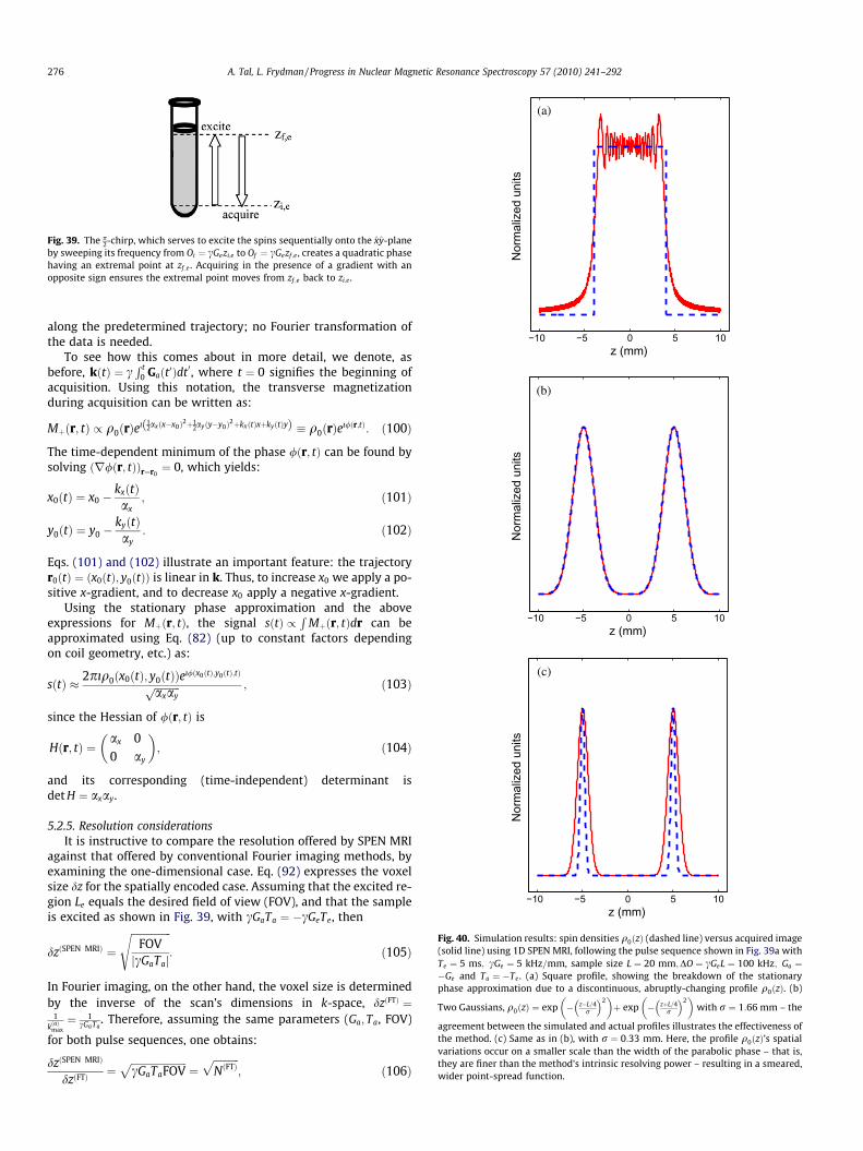
Fig. 39. The p2-chirp, which serves to excite the spins sequentially onto the xy-plane
by sweeping its frequency from Oi ¼ cGezi;e to Of ¼ cGezf ;e , creates a quadratic phasehaving an extremal point at zf ;e . Acquiring in the presence of a gradient with anopposite sign ensures the extremal point moves from zf ;e back to zi;e.
−10 −5 0 5 10z (mm)
Nor
mal
ized
uni
ts
(a)
−10 −5 0 5 10z (mm)
Nor
mal
ized
uni
ts
(b)
−10 −5 0 5 10z (mm)
Nor
mal
ized
uni
ts
(c)
Fig. 40. Simulation results: spin densities q0ðzÞ (dashed line) versus acquired image(solid line) using 1D SPEN MRI, following the pulse sequence shown in Fig. 39a withTe ¼ 5 ms; cGe ¼ 5 kHz=mm, sample size L ¼ 20 mm;DO ¼ cGeL ¼ 100 kHz; Ga ¼�Ge and Ta ¼ �Te . (a) Square profile, showing the breakdown of the stationaryphase approximation due to a discontinuous, abruptly-changing profile q0ðzÞ. (b)
Two Gaussians, q0ðzÞ ¼ exp � z�L=4r
� �2� �
þ exp � zþL=4r
� �2� �
with r ¼ 1:66 mm – the
agreement between the simulated and actual profiles illustrates the effectiveness ofthe method. (c) Same as in (b), with r ¼ 0:33 mm. Here, the profile q0ðzÞ’s spatialvariations occur on a smaller scale than the width of the parabolic phase – that is,they are finer than the method’s intrinsic resolving power – resulting in a smeared,wider point-spread function.
276 A. Tal, L. Frydman / Progress in Nuclear Magnetic Resonance Spectroscopy 57 (2010) 241–292
along the predetermined trajectory; no Fourier transformation ofthe data is needed.
To see how this comes about in more detail, we denote, asbefore, kðtÞ ¼ c
R t0 Gaðt0Þdt0, where t ¼ 0 signifies the beginning of
acquisition. Using this notation, the transverse magnetizationduring acquisition can be written as:
Mþðr; tÞ / q0ðrÞeı 12axðx�x0Þ2þ1
2ayðy�y0Þ2þkxðtÞxþkyðtÞyð Þ � q0ðrÞeı/ðr;tÞ: ð100Þ
The time-dependent minimum of the phase /ðr; tÞ can be found bysolving ðr/ðr; tÞÞr¼r0
¼ 0, which yields:
x0ðtÞ ¼ x0 �kxðtÞax
; ð101Þ
y0ðtÞ ¼ y0 �kyðtÞay
: ð102Þ
Eqs. (101) and (102) illustrate an important feature: the trajectoryr0ðtÞ ¼ ðx0ðtÞ; y0ðtÞÞ is linear in k. Thus, to increase x0 we apply a po-sitive x-gradient, and to decrease x0 apply a negative x-gradient.
Using the stationary phase approximation and the aboveexpressions for Mþðr; tÞ, the signal sðtÞ /
RMþðr; tÞdr can be
approximated using Eq. (82) (up to constant factors dependingon coil geometry, etc.) as:
sðtÞ � 2pıq0ðx0ðtÞ; y0ðtÞÞeı/ðx0ðtÞ;y0ðtÞ;tÞffiffiffiffiffiffiffiffiffiffiaxayp ; ð103Þ
since the Hessian of /ðr; tÞ is
Hðr; tÞ ¼ax 00 ay
� �; ð104Þ
and its corresponding (time-independent) determinant isdet H ¼ axay.
5.2.5. Resolution considerationsIt is instructive to compare the resolution offered by SPEN MRI
against that offered by conventional Fourier imaging methods, byexamining the one-dimensional case. Eq. (92) expresses the voxelsize dz for the spatially encoded case. Assuming that the excited re-gion Le equals the desired field of view (FOV), and that the sampleis excited as shown in Fig. 39, with cGaTa ¼ �cGeTe, then
dzðSPEN MRIÞ ¼
ffiffiffiffiffiffiffiffiffiffiffiffiffiffiffiffiFOVjcGaTaj
s: ð105Þ
In Fourier imaging, on the other hand, the voxel size is determinedby the inverse of the scan’s dimensions in k-space, dzðFTÞ ¼
1kðaÞmax¼ 1
cGaTa. Therefore, assuming the same parameters (Ga; Ta, FOV)
for both pulse sequences, one obtains:
dzðSPEN MRIÞ
dzðFTÞ ¼ffiffiffiffiffiffiffiffiffiffiffiffiffiffiffiffiffiffiffiffiffifficGaTaFOV
p¼
ffiffiffiffiffiffiffiffiffiffiNðFTÞ
p; ð106Þ

Fig. 41. Experimental comparison of conventional (a) and spatially-encoded (b)one-dimensional images, presented alongside the respective pulse sequences usedto obtain them. The experiments were carried out on a uniform water-basedpolyacrylamide gel filling a 5 mm NMR tube, doped at its center with a CoCl2
solution. The observation coil was nearly 18.5 mm in length, and the paramagneticdoping led to a low signal-intensity region ca. 3 mm long. Like all remainingexperiments detailed in this review, these measurements were carried out at500 MHz using a Varian iNova NMR console. Note the 5 ms delay times used toensure full decay of the spins in the middle of the sample.
Fig. 42. (a) 2D SPEN MRI-based pulse sequence. The spins are first excited onto thexy-plane with the aid of a p
2 pulse, creating a quadratic phase /ðx; yÞ ¼ 12 axðx� x0Þ2. A
p-chirped pulse in the presence of Gy adds a quadratic phase along the y-axis,/ðx; yÞ ¼ 1
2 axðx� x0Þ2 þ 12 ayðy� y0Þ
2. Simultaneous purge gradients add linear com-ponents and ensure that /ðx; yÞ has an extremal point at A, shown in (b). Theextremal point is shifted during acquisition – once again, using gradients – to sweepthe path shown in (b). Note that although formally one might say kðtÞ ¼
R t0 Gaðt0Þdt0
varies, the acquisition path is traced in real (as opposed to Fourier) space.
A. Tal, L. Frydman / Progress in Nuclear Magnetic Resonance Spectroscopy 57 (2010) 241–292 277
where NðFTÞ is the number of voxels acquired in the conventional
imaging experiment, NðFTÞ ¼ kðaÞmaxdk ¼
cGaTa
FOV�1. Eq. (106) entails a signifi-cant penalty, whose resolution is further discussed below.
5.2.6. Super-resolutionEq. (106) highlights the main drawback of the spatial encoding
protocol discussed in Section 5.2, compared to conventional Fou-
rier-based MRI: its resolution per unit gradient is lower. Equiva-lently stated, the point-spread function offered by the spatiallyencoded methods relying on a simple magnitude signal calculationwill, for a given set of imaging parameters (Ga; Ta and FOV), be
ffiffiffiffiNp
larger than the Fourier voxel size (given by 1kmax¼ 1
cGaTa).
An implicit assumption leading to this conclusion is that thenumber of voxels along the spatially-encoded direction equalsNUF � FOV
dz , where dz is given by Eq. (105). While it is true that theintrinsic width of the point-spread-function in SPEN MRI is givenby dz, it is, in fact, possible to oversample the image, by shiftingthe quadratic phase in spatial increments smaller than dz whileconstantly acquiring data. The resulting signal (given, for example,by Eq. (91) in 1D), would still remain proportional to the spin den-sity being sought, but it would now contain redundancy; that is, itmay substantially exceed the number of voxels NUF. This redun-dancy can be exploited to increase the image’s resolution well be-yond that given by dz in Eq. (105). Exploiting such redundancy is anexample of ‘‘super-resolution” processing, whose details are out-lined in this section for the 1D case.
The signal at times tk ¼ kdt; k ¼ 1;2; . . . ;M, given in 1D by Eq.(91), can be approximated by replacing the spatial integration overthe sample by a discrete sum of the form
sðtkÞ �XNSR
p¼1
Mþðzp; tkÞDz ¼XNSR
p¼1
q0ðzpÞeı/ðzp ;tkÞDz; ð107Þ
where NSR is the number of discrete elements used to approximatethe integral, Dz ¼ FOV
NSR;q0ðzÞ is the sought-after spin density, and
/ðz; tÞ � /eðzÞ þ /aðz; tÞ is the acquisition phase of the signal, givenby the sum of the quadratic phase /eðzÞ induced by the excitationchirp and the gradient-induced acquisition phase /aðz; tÞ ¼ kðtÞz.Eq. (107) is equivalent to a matrix equation of the form
sðt1Þsðt2Þ. . .
sðtMÞ
0BBB@1CCCA ¼ M NSR
matrix
0BBB@1CCCA
qðz1Þqðz2Þ. . .
qðzNSR Þ
0BBB@1CCCA: ð108Þ
That is, s ¼ Pq, with s and q being column vectors and P an M NSR
matrix which depends solely on the a-priori known acquisitionparameters. Recovering the column vector q is a matter of invertingEq. (108), using, for example, iterative gradient-descent methods tominimize the error of the solution [65]. This approach is one exam-ple of the use of oversampling to achieve ‘‘super-resolution”. Still,since the time signal sðtkÞ is also accompanied by noise, care mustbe taken with regard to the stability and accuracy of the numericaloperations. In the present instance, the inversion of Eq. (108) is par-ticularly well-conditioned, owing to the parabolic phase character-izing the matrix P.
The number of individual equations in Eq. (108) is given by M,the number of time points, while the number of voxels sought afterin the super-resolved image is given by NSR, a free parameter. ForNSR > M – that is, if forcing a search for more spatial points thanthere are temporal ones – unstable solutions result. In practice,the limit NSR ¼ M is found to be often achievable. Thus, using over-sampling, the number of voxels can be made equal to the numberof acquired points, making it dependent on the acquisition param-eters as in conventional Fourier imaging. This can easily offset thehandicap encompassed by Eq. (106), as illustrated by the simplesynthetic patterns shown in Fig. 44.
5.3. Hybrid imaging techniques
Fourier and spatially-encoded imaging have different strengths.Eq. (106) shows that Fourier imaging offers superior resolution perunit gradient during acquisition. As discussed below, however,
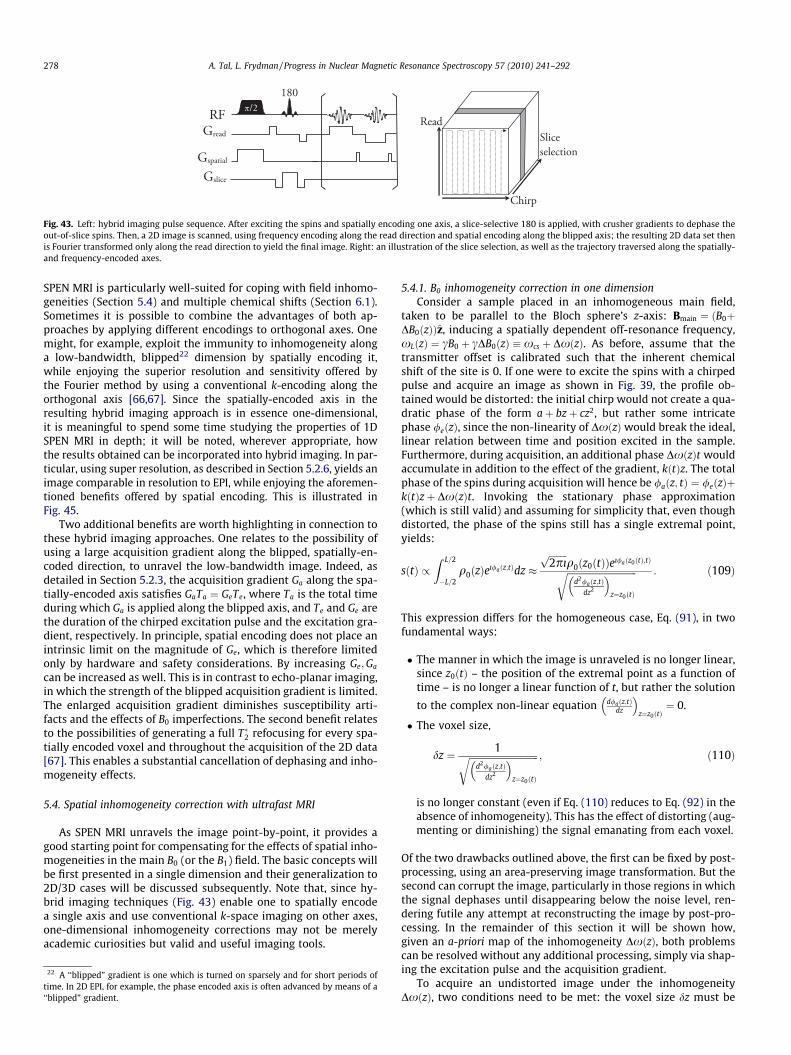
Fig. 43. Left: hybrid imaging pulse sequence. After exciting the spins and spatially encoding one axis, a slice-selective 180 is applied, with crusher gradients to dephase theout-of-slice spins. Then, a 2D image is scanned, using frequency encoding along the read direction and spatial encoding along the blipped axis; the resulting 2D data set thenis Fourier transformed only along the read direction to yield the final image. Right: an illustration of the slice selection, as well as the trajectory traversed along the spatially-and frequency-encoded axes.
278 A. Tal, L. Frydman / Progress in Nuclear Magnetic Resonance Spectroscopy 57 (2010) 241–292
SPEN MRI is particularly well-suited for coping with field inhomo-geneities (Section 5.4) and multiple chemical shifts (Section 6.1).Sometimes it is possible to combine the advantages of both ap-proaches by applying different encodings to orthogonal axes. Onemight, for example, exploit the immunity to inhomogeneity alonga low-bandwidth, blipped22 dimension by spatially encoding it,while enjoying the superior resolution and sensitivity offered bythe Fourier method by using a conventional k-encoding along theorthogonal axis [66,67]. Since the spatially-encoded axis in theresulting hybrid imaging approach is in essence one-dimensional,it is meaningful to spend some time studying the properties of 1DSPEN MRI in depth; it will be noted, wherever appropriate, howthe results obtained can be incorporated into hybrid imaging. In par-ticular, using super resolution, as described in Section 5.2.6, yields animage comparable in resolution to EPI, while enjoying the aforemen-tioned benefits offered by spatial encoding. This is illustrated inFig. 45.
Two additional benefits are worth highlighting in connection tothese hybrid imaging approaches. One relates to the possibility ofusing a large acquisition gradient along the blipped, spatially-en-coded direction, to unravel the low-bandwidth image. Indeed, asdetailed in Section 5.2.3, the acquisition gradient Ga along the spa-tially-encoded axis satisfies GaTa ¼ GeTe, where Ta is the total timeduring which Ga is applied along the blipped axis, and Te and Ge arethe duration of the chirped excitation pulse and the excitation gra-dient, respectively. In principle, spatial encoding does not place anintrinsic limit on the magnitude of Ge, which is therefore limitedonly by hardware and safety considerations. By increasing Ge;Ga
can be increased as well. This is in contrast to echo-planar imaging,in which the strength of the blipped acquisition gradient is limited.The enlarged acquisition gradient diminishes susceptibility arti-facts and the effects of B0 imperfections. The second benefit relatesto the possibilities of generating a full T�2 refocusing for every spa-tially encoded voxel and throughout the acquisition of the 2D data[67]. This enables a substantial cancellation of dephasing and inho-mogeneity effects.
5.4. Spatial inhomogeneity correction with ultrafast MRI
As SPEN MRI unravels the image point-by-point, it provides agood starting point for compensating for the effects of spatial inho-mogeneities in the main B0 (or the B1) field. The basic concepts willbe first presented in a single dimension and their generalization to2D/3D cases will be discussed subsequently. Note that, since hy-brid imaging techniques (Fig. 43) enable one to spatially encodea single axis and use conventional k-space imaging on other axes,one-dimensional inhomogeneity corrections may not be merelyacademic curiosities but valid and useful imaging tools.
22 A ‘‘blipped” gradient is one which is turned on sparsely and for short periods oftime. In 2D EPI, for example, the phase encoded axis is often advanced by means of a‘‘blipped” gradient.
5.4.1. B0 inhomogeneity correction in one dimensionConsider a sample placed in an inhomogeneous main field,
taken to be parallel to the Bloch sphere’s z-axis: Bmain ¼ ðB0þDB0ðzÞÞz, inducing a spatially dependent off-resonance frequency,xLðzÞ ¼ cB0 þ cDB0ðzÞ � xcs þ DxðzÞ. As before, assume that thetransmitter offset is calibrated such that the inherent chemicalshift of the site is 0. If one were to excite the spins with a chirpedpulse and acquire an image as shown in Fig. 39, the profile ob-tained would be distorted: the initial chirp would not create a qua-dratic phase of the form aþ bzþ cz2, but rather some intricatephase /eðzÞ, since the non-linearity of DxðzÞwould break the ideal,linear relation between time and position excited in the sample.Furthermore, during acquisition, an additional phase DxðzÞt wouldaccumulate in addition to the effect of the gradient, kðtÞz. The totalphase of the spins during acquisition will hence be /aðz; tÞ ¼ /eðzÞþkðtÞzþ DxðzÞt. Invoking the stationary phase approximation(which is still valid) and assuming for simplicity that, even thoughdistorted, the phase of the spins still has a single extremal point,yields:
sðtÞ /Z L=2
�L=2q0ðzÞeı/aðz;tÞdz �
ffiffiffiffiffiffiffiffi2pıp
q0ðz0ðtÞÞeı/aðz0ðtÞ;tÞffiffiffiffiffiffiffiffiffiffiffiffiffiffiffiffiffiffiffiffiffiffiffiffiffiffiffiffiffiffid2/aðz;tÞ
dz2
� �z¼z0ðtÞ
r : ð109Þ
This expression differs for the homogeneous case, Eq. (91), in twofundamental ways:
� The manner in which the image is unraveled is no longer linear,since z0ðtÞ – the position of the extremal point as a function oftime – is no longer a linear function of t, but rather the solution
to the complex non-linear equation d/aðz;tÞdz
� �z¼z0ðtÞ
¼ 0.
� The voxel size,
dz ¼ 1ffiffiffiffiffiffiffiffiffiffiffiffiffiffiffiffiffiffiffiffiffiffiffiffiffiffiffiffiffiffid2/aðz;tÞ
dz2
� �z¼z0ðtÞ
r ; ð110Þ
is no longer constant (even if Eq. (110) reduces to Eq. (92) in theabsence of inhomogeneity). This has the effect of distorting (aug-menting or diminishing) the signal emanating from each voxel.
Of the two drawbacks outlined above, the first can be fixed by post-processing, using an area-preserving image transformation. But thesecond can corrupt the image, particularly in those regions in whichthe signal dephases until disappearing below the noise level, ren-dering futile any attempt at reconstructing the image by post-pro-cessing. In the remainder of this section it will be shown how,given an a-priori map of the inhomogeneity DxðzÞ, both problemscan be resolved without any additional processing, simply via shap-ing the excitation pulse and the acquisition gradient.
To acquire an undistorted image under the inhomogeneityDxðzÞ, two conditions need to be met: the voxel size dz must be

Fig. 44. The ability of the super-resolution algorithm to restore high-definition 2D MR images in the presence of noise. (a) Initial synthetic profile containing the target to beresolved. (b) Image arising from simulating the effects of the sequence illustrated in Fig. 43, to which random noise was added to bring the effective SNR to about 5. Dataprocessing consisted of a 1D FT along the read-out axis, and an j SðtÞ jmodulus calculation of the resulting signal. (c) 2D profile arising upon applying the SR algorithm to thedata in (b). Images reproduced from [77].
Fig. 45. In-vivo scans of a mouse brain (FOV ¼ 15 mm 15 mm, compared for several pulse sequences. (a) Single-scan hybrid imaging. The sequence is shown in Fig. 43. A3 ms chirp was used with a 37 kHz/ms sweep rate. The slice selection pulse took 4 ms, with a slice thickness of 0.5 mm. Total acquisition time was 15 ms, resulting in voxelsizes of 0.5 mm along both the spatially and frequency encoded axes. (b) Same as in (A), after employing super-resolved reconstruction along the spatially-encoded axis. (c)Single-scan spin echo EPI (1 mm slice, with voxel sizes of 0:5 mm 0:65 mm, and a total sequence duration of 24 ms). (d) A reference multi-scan Gradient-Echo image(acquisition time = 30 s). Images reproduced from [77].
23 It is d/edz , and not /eðzÞ, which ultimately is physically meaningful (see Eq. (124)), as
an additional constant phase has no effect on the relative phasing and dephasing ofthe spins.
A. Tal, L. Frydman / Progress in Nuclear Magnetic Resonance Spectroscopy 57 (2010) 241–292 279
time-independent, and the acquisition path z0ðtÞmust be, as in thehomogeneous case, linear with time:
z0ðtÞ ¼ zf ;e �zf ;e � zi;e
Ta
� �t: ð111Þ
Since
d/aðz; tÞdz
¼ d/eðzÞdz
þ kðtÞ þ dDxðzÞdz
t; ð112Þ
d2/aðz; tÞdz2 ¼ d2/eðzÞ
dz2 þ d2DxðzÞdz2 t; ð113Þ
the demand dz ¼ const: can be recast, using Eqs. (113) and (110), as:
d2/eðzÞdz2 þ d2DxðzÞ
dz2 t
!z¼z0ðtÞ
¼ 1dz2 ¼ const: ð114Þ
This furnishes a differential equation for /eðzÞ. Furthermore,demanding that z0ðtÞ be linear is equivalent to demanding thatEq. (111) be the solution of d/aðz;tÞ
dz ¼ 0. By Eq. (112), that demandcan be satisfied by choosing kðtÞ, and hence the acquisition gradientcGaðtÞ ¼ dk
dt, to be:
kðtÞ ¼ � d/eðzÞdz
þ dDxðzÞdz
t� �
z¼z0ðtÞ: ð115Þ
This dictates the form of GaðtÞ. To sum up, one can recover theundistorted image by suitably exciting the sample with the appro-priate /eðzÞ and by shaping the acquisition gradient GaðtÞ accordingto Eqs. (115) and (114). The explicit form of these two quantitieswill be derived next.
Throughout the acquisition process there is a one-to-one corre-spondence between the position of a voxel and the time at which itis unraveled: t can thus be considered as a function of z, and Eq.(111) can consequently be inverted to give tðzÞ ¼ Ta
Leðz� zf ;eÞ.
Hence:
ddt¼ dz
dtddz¼ � Le
Ta
ddz: ð116Þ
Based on this, it is possible to recover /eðzÞ by integrating Eq. (114)twice. Of the two integration constants this demands, one is anoverall constant phase and is physically irrelevant; the other canbe obtained by recalling that, at the beginning of the acquisition,the phase /aðz; t ¼ 0Þ – comprised solely of /eðzÞ at that point intime – will have an extremum at z ¼ zf ;e:
d/eðzÞdz
� �z¼zf ;e
¼ 0: ð117Þ
Using this as a boundary condition, and integrating twice:
/eðzÞ ¼ �DxðzÞtðzÞ � 2Ta
Le
ZDxðzÞdzþ ðz� zf ;eÞ2
2dz2
þ TaDxðzf ;eÞLe
z: ð118Þ
Treating then dz; Ta; Le; zf ;e as given parameters and assuming thatthe inhomogeneity DxðzÞ has been mapped and is known, Eq.(118) completely determines the desired form of the excitationphase.23
To obtain an expression for the acquisition gradient GaðtÞ, wedifferentiate Eq. (115) and use Eq. (116):
cGaðtÞ ¼dkðtÞ
dt¼ � Le
Ta
d2/eðzÞdz2 þ d2DxðzÞ
dz2 t
" #þ dDxðzÞ
dz: ð119Þ
Comparing this with Eq. (114), note that the term in the squarebracket is constant and equal to 1
dz2, and hence:
cGaðtÞ ¼ �Le
Tadz2 þdDxðzÞ
dz; ð120Þ
which yields a closed form solution for GaðtÞ.While GaðtÞ can be easily shaped using modern hardware
according to Eq. (120), it still remains to be shown how one can

280 A. Tal, L. Frydman / Progress in Nuclear Magnetic Resonance Spectroscopy 57 (2010) 241–292
excite a sample with the appropriate phase, given by Eq. (118). Tothis end a non-linear swept pulse has to be employed which, like achirped pulse, excites the spins sequentially but no longer in a z / tlinear fashion. The analysis of such pulses closely follows and gen-eralizes that of Section 2.2.1. Indeed, a chirped pulse is character-ized by an instantaneous angular frequency, xcðtÞ, which isrelated to its phase by /cðtÞ ¼
R t0 xcðtÞdt. Consider a sample with
a spatially dependent off-resonance frequency xLðzÞ, the result ofan excitation gradient Ge and some spatial inhomogeneity:xLðzÞ ¼ cGezþ DxðzÞ. A properly calibrated chirped pulse will ex-cite the spins onto the xy-plane with a phase /eðzÞ. To compute thisphase, one can use Eq. (13), which is valid even in the non-linearcase; the non-linearity is then implicitly contained in xLðzÞ andin tz, the time at which the chirped pulse excites the spin posi-tioned at z.
To infer the desired form of xcðtÞ and tz in this inhomogeneouscase, we demand that Eq. (13) be equal to the desired phase profile/eðzÞ given by Eq. (118). Differentiating these equations on bothsides yields:
d/cðtzÞdz
þ dxLðzÞdz
ðTe � tzÞ �xLðzÞdtz
dz¼ d/eðzÞ
dz: ð121Þ
where, by the rules of differentiation
d/cðtzÞdz
¼ ddz
Z tz
0xcðt0Þdt0 ¼ dtz
dz:xcðtzÞ: ð122Þ
Note that xcðtzÞ is the frequency of the chirp at the point in time inwhich it excites the spin at z, the off-resonance frequency of whichis xLðzÞ. Since the chirp excites those spins that match its instanta-neous frequency, one must have xcðtzÞ ¼ xLðzÞ. Substituting thisinto Eq. (121) and simplifying, one gets:
dxLðzÞdz
ðTe � tzÞ ¼d/eðzÞ
dz: ð123Þ
Solving for tz yields:
tz ¼ Te �d/eðzÞ
dzdxLðzÞ
dz
: ð124Þ
This yields the desired form of tz. Such relation can be inverted, inmost cases numerically, to yield zt , the position in the sample ex-cited at a given time t. This can then be used to determine xcðtÞ,since:
xcðtÞ ¼ xLðztÞ: ð125Þ
Eq. (125) merely expresses the requirement on the chirp to excitethe spins at zt at time t. All that remains to be done is to properlycalibrate the chirped pulse such that all spins will get preciselytipped onto the xy-plane. Using a constant irradiation amplitudeas shown in Fig. 4a will not suffice, as the non-linear sweep of thepulse means different regions in the sample will be affected for dif-ferent amounts of time. Eq. (15), though, remains valid, providedthe constant rate R is generalized to dxc
dt , the instantaneous rate.24
Fig. 46 presesnts an experimental example of how those consider-ations can restore the integrity of a NMR image.
5.4.2. Generalization to higher dimensionsThe techniques outlined in Section 5.4.1 can be generalized to
higher dimensions, with a few caveats. Assuming the spins havebeen excited onto the xy-plane with a phase /eðrÞ, they will accu-mulate a phase /aðr; tÞ ¼ /eðrÞ þ kðtÞ � rþ DxðrÞt throughoutacquisition. In two dimensions the acquired signal will be:
24 This reduces to R in the case of a linear chirp.
sðtÞ ¼Z
q0ðrÞeı/aðr;tÞdr � 2pıq0ðr0ðtÞÞeı/aðr0ðtÞ;tÞffiffiffiffiffiffiffiffiffiffiffiffiffiffiffiffiffiffiffiffiffiffiffiffiffiffidetðHÞr¼r0ðtÞ
q ; ð126Þ
where r0ðtÞ is the trajectory of the stationary point, given implicitlyby ðr/aðr; tÞÞr¼r0ðtÞ ¼ 0. H is the Hessian of /aðr; tÞ, as evaluatedalong r0ðtÞ:
HðrÞ ¼@xx @xy
@yx @yy
� �/aðr; tÞ ¼
@xx @xy
@yx @yy
� �/eðrÞ þ DxðrÞtð Þ: ð127Þ
As with the one-dimensional case, artifacts will be introduced intothe image via two routes: The acquisition trajectory r0ðtÞ mightdeviate from the ideal, and the pixel size
dV � 2pffiffiffiffiffiffiffiffiffiffiffiffiffiffiffiffiffiffiffiffiffiffiffiffiffiffidetðHÞr¼r0ðtÞ
q ; ð128Þ
might be time-dependent. Fortunately, the approaches for correct-ing them outlined for the one-dimensional experiment (Sec-tion 5.4.1) are applicable here as well: to force a particulartrajectory r0ðtÞ, the acquisition gradients GaðtÞ must be shaped,and to ensure dV is time independent, the excitation phase/eðx; yÞ must be tailored accordingly.
Assuming /eðrÞ has been computed, the first requirement isstraightforward to implement, by demanding r0ðtÞ is the stationarypoint of /aðr; tÞ for all t:
r/aðr; tÞð Þr¼r0ðtÞ ¼ 0: ð129Þ
kðtÞ can be solved for explicitly by substituting /aðr; tÞ ¼ /eðr; tÞþkðtÞ � rþ DxðrÞt, giving
kðtÞ ¼ � r/eðrþrDxðrÞt½ �r¼r0ðtÞ: ð130Þ
As all quantities on the RHS are known, kðtÞ can be determined inclosed form via straightforward differentiation. Furthermore, /eðrÞcan be found by demanding that dV (Eq. (128)), which dependson /eðrÞ implicitly, be constant. Unlike the one-dimensional case,in which there exists a 1–1 relation between time and position(Eq. (116)), iterative numerical schemes must be employed in thegeneral case to find /eðrÞ. An analytical solution is, however, possi-ble for some cases [11]. Fig. 47 shows an experimental example ofsuch an instance.
5.5. Signal-to-noise and noise filtering in SPEN MRI
An important feature to compare is the signal to noise ratio ofconventional Fourier imaging against SPEN MRI. This will be dis-cussed using the case of 1D image acquisition as a framework.As with the spectroscopic case (Section 3.3.4), we shall assumesome statistically random and additive noise nðtÞ to be presentin addition to the signal sðtÞ originating from the spins. The SNRis defined as
SNR � srms
nrms: ð131Þ
The subscript rms stands for root-mean-square, and for a signal f ðtÞ
of duration T is defined as frms �ffiffiffiffiffiffiffiffiffiffiffiffiffiffiffiffiffiffiffiffiffiffiffiffiffiffiffi1T
R T0 jf ðtÞj
2dtq
. Comparing the SNRs
of both SPEN MRI and FT imaging involves the computation of thequantity:
SNRðSPEN MRIÞ
SNRðFTÞ ¼ sðSPEN MRIÞrms
sðFTÞrms
nðFTÞrms
nðSPEN MRIÞrms
: ð132Þ
It is often the case in imaging that one is interested in the signal tonoise per voxel. For a meaningful comparison the field-of-view(FOV) and the voxel size ðdzÞ will be taken to be the same in bothexperiments: dzðSPEN MRIÞ ¼ dzðFTÞ � dz; FOVðSPEN MRIÞ ¼ FOVðFTÞ � L.

Fig. 46. 1D spatially-encoded imaging in inhomogeneous fields: experimental results. All experiments were carried out on a 500 MHz iNova NMR spectrometer. The sampleis described in Fig. 41. (a and b) FT and spatially-encoded profiles collected from the phantom under conditions similar to those detailed in that figure: 5 G/cm excitation andacquisition gradients, 10 ms average free-evolution times, 18.5 mm long samples, etc. (c and d) As in (a and b), but upon subjecting on the sample to an artificialXinh ¼ 1:31zþ 0:193z2 kHz (with z the displacement away from the sample’s center in mm). This inhomogeneity was introduced by distorting the z; z2 magnet shims, and wascharacterized by mapping the water resonance using a simple gradient-echo sequence. (e) Idem as in (d) but after inserting the mapped inhomogeneity profile into thealgorithm described in the text, recalculating from it the correcting RF sweep and acquisition gradient patterns, and applying these for the acquisition of the data. The mostremarkable feature of this compensation procedure (and therefore a basic test of its correct functioning) is that it enabled the signal to endure in the time-domain, long aftereither the conventional k-space or its analogous spatially-encoded signal have both decayed into the background noise. This, in spite of Xinh spanning over 25 kHz and of theexperiment still requiring Ge ¼ 5 G=cm, and an average Ga ¼ þ4:13 G=cm over the acquisition. Notice that although still not ideal, the wiggles exhibited by this experimentalXinh-compensated profile are akin to those of its homogeneous counterpart in (b). Simulations indicate that these reflect in both cases limitations of the chirped excitationpulse in delivering the desired profile, rather than in an actual failure of the compensation procedure.
A. Tal, L. Frydman / Progress in Nuclear Magnetic Resonance Spectroscopy 57 (2010) 241–292 281
Letting kðSPEN MRIÞmax � cGðSPEN MRIÞ
a TðSPEN MRIÞa ; kðFTÞ
max � cGðFTÞa TðFTÞ
a andequating voxel sizes, one obtains
ffiffiffiffiffiffiffiffiffiffiffiffiffiffiffiffiL
kðSPEN MRIÞmax
q¼ ðkðFTÞ
max�1, or simply:
kðSPEN MRIÞmax ¼ NkðFTÞ
max; ð133Þ
where L kðFTÞmax ¼ N is the number of voxels – the same in both
experiments. The experimental acquisition time Ta will be takento be equal in both cases, so as to equalize the effects of relaxation;hence, Eq. (133) becomes
GðSPEN MRIÞa ¼ NGðFTÞ
a : ð134Þ
Since GðSPENMRIÞa > GðFTÞ
a , one must use a larger filter bandwidth duringSPEN MRI; and since the noise level increases as the square root ofthe filter bandwidth:
nðFTÞrms
nðSPEN MRIÞrms
¼
ffiffiffiffiffiffiffiffiffiffiffiffiffiffiffiffiffiffiffiffiffiGðFTÞ
a
GðSPEN MRIÞa
s¼ 1ffiffiffiffi
Np : ð135Þ
Signal levels can be similarly compared. From Eq. (91), the rms sig-nal in a single voxel is jsðSPEN MRIÞ
rms j / M0ðz0ðtÞÞdzðSPEN MRIÞ up to someproportionality constant which depends on the receiver geometryand electronics (and is hence shared by both experiments). It canbe similarly shown [68] that for a single voxel jsðFTÞ
rms j / M0ðzÞdzðFTÞ.Since voxel sizes have been chosen to be equal, sðFTÞ
rms ¼ sðSPEN MRIÞrms ,
and as a result
SNRðSPEN MRIÞ
SNRðFTÞ ¼ffiffiffiffi1N
r: ð136Þ
That is, spatial encoding suffers affiffiffiffiNp
reduction in its SNR comparedto Fourier imaging, where N is the number of voxels. This, however,can be remedied and brought up-to-par by suitable post-processing.In what follows, we shall assume that the magnitude jsðtÞj of the ac-quired SPEN MRI signal, which is proportional to the image, will beused; any phase information will be considered superfluous. It willalso be convenient to employ the time-axis instead of the spatial z-axis to describe the procedure. For the sake of simplicity, the treat-ment will remain confined to the one-dimensional case.
In the beginning of an experiment, the filter bandwidth of theNMR receiver needs to be properly set. If set too high, and exces-sive noise will be introduced into the signal, whereas if set toolow, relevant frequencies will be filtered out. For SPEN MRI, the
range of essential frequencies is determined by the difference infrequencies between the first and last voxels, situated at L
2. Thespatially dependent off-resonance frequency, xLðzÞ ¼ cGaz, dic-tates this difference to be xL þ L
2
� ��xL � L
2
� �¼ cGaL; thus one must
set fbw ¼ cGaL, which then sets the acquisition dwell time to 1fbw.
The main insight into reducing noise levels is shown in Fig. 48:while fbw ¼ cGaL, the actual signal emanates from a small regionof width dz, equal to the voxel size; all other spins are dephasedby the rapidly changing quadratic phase. Since noise levels in thesample are proportional to
ffiffiffiffiffiffiffiffiffifbwp
, it would be desirable to reducefbw from cGaL by a factor of N to cGadz. In principle, this is not pos-sible, since the instantaneous frequencies of the voxels will spanthe entire range cGaL throughout the acquisition. There is, how-ever, no imaging information encoded in this frequency spread.By suitable post-processing it is thus possible to localize the voxelsin frequency space into a narrow band of frequencies of widthcGadz, while filtering out the extraneous noise outside it.
The filtering process shown schematically in Fig. 49, and theensuing SNR gains, can be understood as follows: the SPEN MRI im-age is the sum of noise and of the coherent signal of the image.Spectrally, the noise is white and spans a range of frequencies gi-ven by the fbw. However, the signal being sought, whose charac-teristic scale of change of which is set by the voxel size dz, spansa much smaller range of frequencies. Denoting by dt the smallesttime-scale associated with the image (see Fig. 49a), it follows thatthe FT of the coherent signal of the image then occupies a regionnot any larger than 1
dt. Since the z and t axes are linearly relatedin 1D SPEN MRI, dt is proportional to the voxel size. In fact,
Ta
dt¼ L
dz¼ N; ð137Þ
where N is the number of voxels, and so, using Eq. (105):
1dt¼ cGaL
N¼ fbw
N: ð138Þ
With this insight, a filtering procedure to optimize the SPEN SNRbecomes straightforward: Any noise outside of a spectral width 1
dtshould be removed via a windowing-function (Fig. 49c) and theresulting filtered spectrum should be Fourier transformed back tothe time-domain (Fig. 49d) to retrieve the desired, filtered image.

Fig. 47. 2D spatially-encoded imaging in inhomogeneous fields: experimental results. The images were obtained on the same phantom sample used in Figs. 46 and 41. (a)Single-scan 2D FT EPI image recorded using a blipped read-out of 32 echoes spread over 32 ms; acquisition gradients were Gy ¼ 15 G=cm; Gx ¼ 0:85 G=cm (see Fig. 35)(pulsed over 50 ls every 950 ls). (b) Single-scan 2D spatially-encoded image collected using a zigzagging scheme as in Fig. 42 with Gy ¼ 15 G=cm; Gx ¼0:85 G=cm; Ny ¼ 16 and an excitation gradient of 4 G/cm. (c and d) Idem as in (a and b) but upon subjecting the sample to the artificial inhomogeneity XinhðzÞ ¼0:023z2 þ 0:025z. (e) Idem as in (d), after applying the correction algorithm described in the text.
Fig. 48. In SPEN MRI, the filter bandwidth must be set to cover the entire sample,cGaL, since the instantaneous frequency of each voxel varies throughout acquisition,from � cGa L
2 to cGa L2 . However, at each instant, only a small range of frequencies –
those originating from within the current voxel dz – comprise the signal.
282 A. Tal, L. Frydman / Progress in Nuclear Magnetic Resonance Spectroscopy 57 (2010) 241–292
As the spectral components of the coherent time-domain signal ofthe image are not disturbed, the image quality is preserved, whilethe noise’s bandwidth is decreased by a factor of N. The gain inSNR afforded by the filtering procedure is due to the reduction inthe noise level: The filter bandwidth has been effectively truncatedby a factor of N. Since the noise scales as
ffiffiffiffiffiffiffiffiffifbwp
, this implies a gain offfiffiffiffiNp
in the SNR. Note that, by Eq. (136), this renders the SNR of SPENMRI comparable to that of Fourier-based imaging methods.
6. Spectroscopic aspects of ultrafast MRI and spatial aspects ofultrafast 2D NMR
Spatially encoded 2D NMR and MRI share a common reliance onfrequency-swept pulses, applied in the presence of field gradientsso as to encode the spin interactions. It turns out that, as a resultof this, spatially-encoded images carry within them spectroscopicinformation, and spatially-encoded spectra also carry the imageof the spins in the sample. In both cases, the complementary spec-tral/spatial information arises at no extra cost in the experimentalcomplexity: it simply resides in the signal, whether we are inter-ested in it or not. The extraction of this additional information isthe topic of the current section. First, in Section 6.1 it will be exam-ined how one can extract different images from differing chemicalsites, a problem known as chemical shift imaging (CSI). In Sec-tion 6.1.1 it will be shown that hybrid imaging (see Section 5.3)can be used to carry out a CSI experiment in n-dimensions. Theextension of those ideas to cases involving inhomogeneous B0
fields will be briefly touched upon in Section 6.1.2. Following thediscussion of CSI, in Section 6.2 the inverse problem will then bestudied, namely, the extraction of a two-dimensional spectrum ofa sample by imaging that sample. This leads to a UF2DNMR spec-troscopy method based on a single-sweep of the spins.
6.1. Chemical shift imaging
This section builds upon the concepts introduced in Sec-tion 5.5, and shows how the phase of a SPEN MRI sðtÞ signalcan be utilized to spectrally separate images stemming frommedia with different chemical shifts, such as fat and water in tis-sues. This could allow for the chemical shift imaging (CSI)[69,39,70] of all sources in the sample, using post-processing toreconstruct the multidimensional images arising from every
chemical site, simultaneously and within a single-scan. SPENMRI is particularly well suited to accomplish this, as it does notrequire a modification of the original pulse sequence – it only re-quires using the hitherto disregarded phase of the signal. This isunlike EPSI-type techniques used in Fourier-based spectroscopicimaging, which require introducing an additional alternation ofthe gradient (and hence an additional dimension [39]), in orderto spectrally resolve each peak of interest. In this section, thechemical shift xcs will no longer be assumed zero. Starting forsimplicity with the one-dimensional case, generalizations tomore dimensions will be presented later.
The phase of the spins following a p2-chirped pulse is given by Eq.
(14). If one were to acquire now the signal while applying a gradi-ent Ga, the stationary point z0ðtÞ would follow a trajectory definedby: d
dz ½/eðzÞ þ cGatzþxcst�z¼z0ðtÞ ¼ 0. Setting R � ExcitedFrequencyRrange2pTe
¼cGeL2pTe
, GaTa ¼ �GeTe, and then solving for z0ðtÞ, one obtains:
z0ðtÞ ¼L2
1� 2tTa
� �� xcs
cGe: ð139Þ
We see that the effect of the chemical shift is to slightly shift the ac-quired region by an amount Dz ¼ xcs
cGe(compare Eq. (139) and (90));
for typical numbers, such as Ge ¼ 1 G/cm and a 100 Hz chemicalshift, this would imply a shift of approximately 0.2 mm for protons.

Fig. 49. Noise filtering in SPEN MRI. (a) The original signal with noise. dt signifies the voxel size along the time axis, which is proportional to the spatial z-axis. (b) The Fouriertransform of the signal in (a). The noise occupies a much larger band of frequencies (given by fbw) when compared to the band occupied by the signal, dt�1. (c) By filtering outthe noise, the effective filter bandwidth is truncated from cGaL to dt�1. (d) Fourier transforming backwards, the image remains unharmed while the noise levels drop by afactor of
ffiffiffiffiffiffifficGa Ldt�1
q¼
ffiffiffiffiNp
, where N is the number of voxels.
25 The stationary point equation, d/ðyÞady ¼ 0 does not contain time explicitly, and hence
the time-dependence of the stationary point enters only implicitly, via its dependenceon kyðtÞ. In the 2D case, the stationary point y0 retains its linearity in ky , even thoughit is no longer linear in time.
A. Tal, L. Frydman / Progress in Nuclear Magnetic Resonance Spectroscopy 57 (2010) 241–292 283
On the other hand, using Eq. (139) to evaluate /aðz0ðtÞ; tÞ, the phaseof the collected signal, one obtains:
/aðz0ðtÞ; tÞ ¼cGeTeL
2T2a
!t2 � cGeTeL
2Ta
� �t
" #þ 1þ Te
Ta
� �xcst: ð140Þ
This /aðz0ðtÞ; tÞ separates naturally into two components: One thatis independent of the chemical shift and one that depends linearlyon it. The chemical-shift independent phase is shared by all spins,regardless of their chemical shift, and can be removed by multiply-ing the total signal by the negative of the phase, e�ıð...Þ. The remain-
ing term, 1þ TeTa
� �xcst � Dmt, modulates the signal by an effective
offset Dm.Consider next the acquisition of such a signal, assuming it orig-
inates from a sample containing q different chemical sites,
xð1Þcs ;xð2Þcs ; . . . ;xðqÞcs , each characterized by a different spin density
qð1Þ0 ðzÞ;qð2Þ0 ðzÞ; . . . ;qðqÞ0 ðzÞ. Neglecting the small dependence of on
the chemical shift of z0ðtÞ noted in Eq. (139), the acquired signal
can be expressed as sðtÞ /Pq
p¼1qðpÞ0 ðz0ðtÞÞeı/aðz0ðtÞ;tÞ. Phase correcting
this signal can remove the above-mentioned phase terms commonto all sites, yielding:
sðtÞ /Xq
p¼1
qðpÞ0 ðz0ðtÞÞeıDmpt; ð141Þ
where Dmp � 1þ TeTa
� �xðpÞcs . The result of such a global ‘‘phase correc-
tion” is akin to the frequency demodulation introduced in Sec-tion 5.5. Recall, from that discussion, that the spectral width ofthe Fourier transform of the image (given by jsðtÞj), is given bythe inverse of the dwell time, chosen to be the filter-bandwidth,fbw ¼ cGaL; hence, the image’s frequency components occupy a re-gion of size cGadz � 1
dt in frequency space (Eq. (138), Fig. 49). TheFourier transform of Eq. (141) merely results in the same spectralcontent for each site p, shifted by an offset Dmp. The filtering proce-dure assumes that this shift is larger than 1
dt, so the spectral contentsoriginating from different chemical sites do not overlap. Under thisassumption, the spectral contents of each site sðpÞðtÞ are distinct, andcan be singled out via a Fourier transform of the spatially encodedFID. Then, by applying a windowing-function to the resulting spec-trum and eliminating all spectral components originating fromsðkÞðtÞ; k–p, one can isolate the response from each chemically-shifted site. Fourier transforming back to the time-domain retrievesonly that part of the image originating from the pth spectral peak:
qðpÞ0 ðzÞ. The procedure is outlined in Fig. 50 for the case of two chem-
ical sites, xð1Þcs ;xð2Þcs , and its net effect is the delivery of a set of chem-
ical shift resolved images.The maximum resolving power of this spectroscopic imaging
method – that is, the closest two chemical shifts it can successfullyseparate – can be estimated by demanding that the shift Dm be lar-ger than the width of the spectral region occupied by each image,1dt. This leads to:
Dxcs PfbwTa
NðTa þ TeÞ: ð142Þ
Taking, as an example, Te ¼ 20 ms; Ta ¼ 0:2 s; Ge ¼ 0:2 Gauss=cm; L ¼ 5 cm, one finds dz ¼ 5 mm and Dxcs P 0:5 kHz.
6.1.1. Hybrid chemical shift imagingThe notions just presented can be generalized to nD imaging by
employing either full nD spatial encoding, or hybrid imaging ap-proaches [12]. We cover here the latter case (illustrated inFig. 43). Fig. 51a illustrates for completeness the 2D data set result-ing from such an experiment: its rows are Fourier-encoded, whileits columns are spatially encoded. By treating the columns as one-dimensional imaging experiments it is possible to apply the samepost-acquisition processing described for a 1D case; the remainderof this section formalizes this notion for the 2D case.
The acquisition phase of the spins as a function of position canbe written, for a 2D hybrid SPEN MRI experiment, as:
/aðx; y; tÞ ¼ /ðxÞe ðxÞ þ kxðtÞxh i|fflfflfflfflfflfflfflfflfflfflfflfflfflffl{zfflfflfflfflfflfflfflfflfflfflfflfflfflffl}
/ðxÞa ðx;kxÞ
þ /ðyÞe ðyÞ þ kyðtÞyh i|fflfflfflfflfflfflfflfflfflfflfflfflfflffl{zfflfflfflfflfflfflfflfflfflfflfflfflfflffl}
/ðyÞa ðy;kyÞ
þxcst; ð143Þ
where /ðxÞe ;/ðyÞe are the phases encoded along the x- and y-axes prior
to acquisition. As the x-axis is Fourier-encoded, /ðxÞe ðxÞ ¼ �cGaDTa;xx
2 isthe linear phase created by the gradient just prior to acquisition;/ðyÞe ðyÞ is the quadratic phase induced by the chirp, as given by Eq.(14) with z replaced by y. The acquired signal is:
sðtÞ ¼Z Z
dxdyq0ðx; yÞeı /ðxÞe ðxÞþkxx½ �þı /ðyÞe ðyÞþkyy½ �þıxcst ; ð144Þ
where the time-dependence of kx; ky has now been made implicit.Since /ðyÞe ðyÞ is quadratic, y can be integrated over by employingthe stationary phase approximation, while treating x; t; kx; ky asconstants:
sðtÞ ¼ffiffiffiffiffiffiffiffi2pıp
eı/ðyÞa ðy0ðkyÞ;kyÞeıxcstdyZ
dxeı /ðxÞe þkxx½ �q0ðx; y0ðkyÞÞ; ð145Þ
where dy is the voxel size along the spatially-encoded axis as givenby Eq. (92) (for z), and y0ðkyÞ � y0ðkyðtÞÞ is the position of the sta-tionary point as a function of25 ky, obtained by solving the following
equation, d/ðyÞady ¼ 0:
y0ðkyÞ ¼ yinitial þLy
cGeTe
� �ky; ð146Þ
yinitial ¼Ly
2� xcs
cGe: ð147Þ
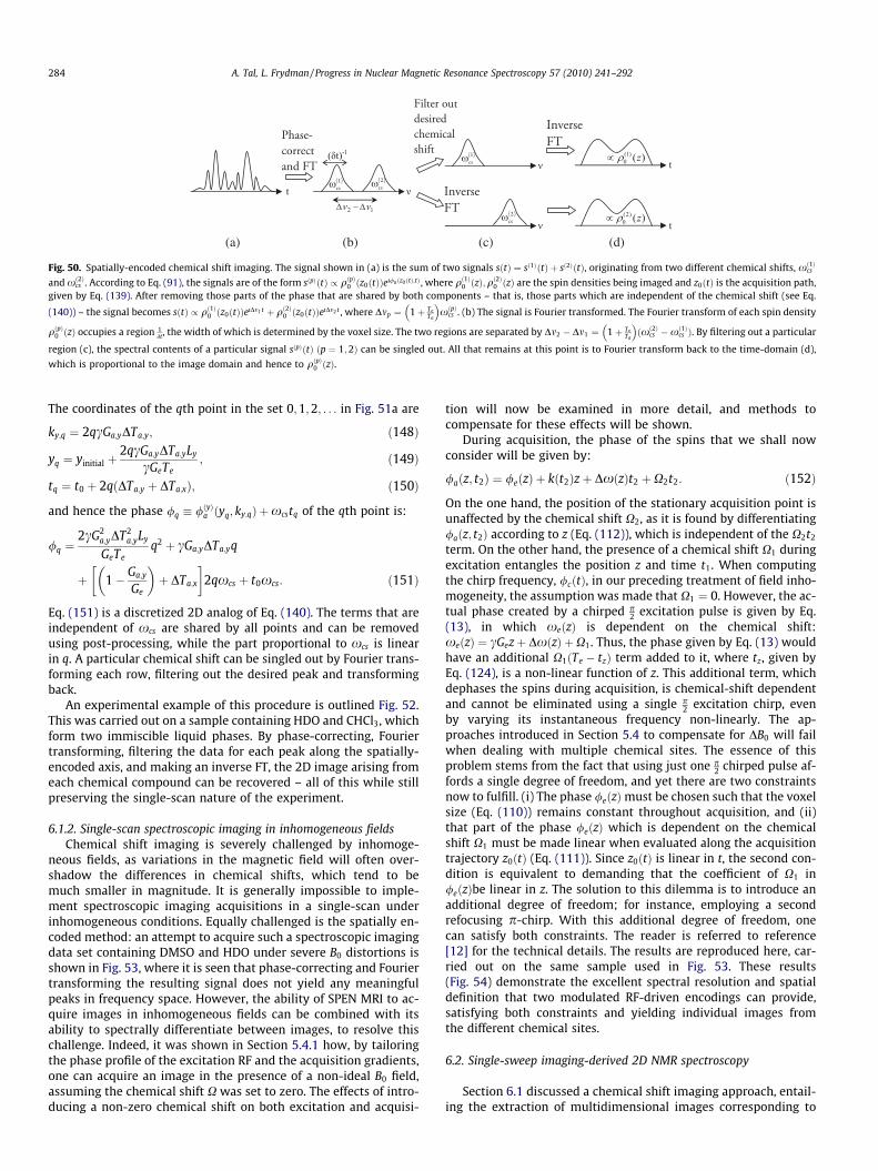
Fig. 50. Spatially-encoded chemical shift imaging. The signal shown in (a) is the sum of two signals sðtÞ ¼ sð1ÞðtÞ þ sð2ÞðtÞ, originating from two different chemical shifts, xð1Þcs
and xð2Þcs . According to Eq. (91), the signals are of the form sðpÞðtÞ / qðpÞ0 ðz0ðtÞÞeı/a ðz0 ðtÞ;tÞ , where qð1Þ0 ðzÞ;qð2Þ0 ðzÞ are the spin densities being imaged and z0ðtÞ is the acquisition path,
given by Eq. (139). After removing those parts of the phase that are shared by both components – that is, those parts which are independent of the chemical shift (see Eq.
(140)) – the signal becomes sðtÞ / qð1Þ0 ðz0ðtÞÞeıDm1 t þ qð2Þ0 ðz0ðtÞÞeıDm2 t , where Dmp ¼ 1þ TeTa
� �xðpÞcs . (b) The signal is Fourier transformed. The Fourier transform of each spin density
qðpÞ0 ðzÞ occupies a region 1dt, the width of which is determined by the voxel size. The two regions are separated by Dm2 � Dm1 ¼ 1þ Te
Ta
� �ðxð2Þcs �xð1Þcs Þ. By filtering out a particular
region (c), the spectral contents of a particular signal sðpÞðtÞ ðp ¼ 1;2Þ can be singled out. All that remains at this point is to Fourier transform back to the time-domain (d),
which is proportional to the image domain and hence to qðpÞ0 ðzÞ.
284 A. Tal, L. Frydman / Progress in Nuclear Magnetic Resonance Spectroscopy 57 (2010) 241–292
The coordinates of the qth point in the set 0;1;2; . . . in Fig. 51a are
ky;q ¼ 2qcGa;yDTa;y; ð148Þ
yq ¼ yinitial þ2qcGa;yDTa;yLy
cGeTe; ð149Þ
tq ¼ t0 þ 2qðDTa;y þ DTa;xÞ; ð150Þ
and hence the phase /q � /ðyÞa ðyq; ky;qÞ þxcstq of the qth point is:
/q ¼2cG2
a;yDT2a;yLy
GeTeq2 þ cGa;yDTa;yq
þ 1� Ga;y
Ge
� �þ DTa;x
�2qxcs þ t0xcs: ð151Þ
Eq. (151) is a discretized 2D analog of Eq. (140). The terms that areindependent of xcs are shared by all points and can be removedusing post-processing, while the part proportional to xcs is linearin q. A particular chemical shift can be singled out by Fourier trans-forming each row, filtering out the desired peak and transformingback.
An experimental example of this procedure is outlined Fig. 52.This was carried out on a sample containing HDO and CHCl3, whichform two immiscible liquid phases. By phase-correcting, Fouriertransforming, filtering the data for each peak along the spatially-encoded axis, and making an inverse FT, the 2D image arising fromeach chemical compound can be recovered – all of this while stillpreserving the single-scan nature of the experiment.
6.1.2. Single-scan spectroscopic imaging in inhomogeneous fieldsChemical shift imaging is severely challenged by inhomoge-
neous fields, as variations in the magnetic field will often over-shadow the differences in chemical shifts, which tend to bemuch smaller in magnitude. It is generally impossible to imple-ment spectroscopic imaging acquisitions in a single-scan underinhomogeneous conditions. Equally challenged is the spatially en-coded method: an attempt to acquire such a spectroscopic imagingdata set containing DMSO and HDO under severe B0 distortions isshown in Fig. 53, where it is seen that phase-correcting and Fouriertransforming the resulting signal does not yield any meaningfulpeaks in frequency space. However, the ability of SPEN MRI to ac-quire images in inhomogeneous fields can be combined with itsability to spectrally differentiate between images, to resolve thischallenge. Indeed, it was shown in Section 5.4.1 how, by tailoringthe phase profile of the excitation RF and the acquisition gradients,one can acquire an image in the presence of a non-ideal B0 field,assuming the chemical shift X was set to zero. The effects of intro-ducing a non-zero chemical shift on both excitation and acquisi-
tion will now be examined in more detail, and methods tocompensate for these effects will be shown.
During acquisition, the phase of the spins that we shall nowconsider will be given by:
/aðz; t2Þ ¼ /eðzÞ þ kðt2Þzþ DxðzÞt2 þX2t2: ð152Þ
On the one hand, the position of the stationary acquisition point isunaffected by the chemical shift X2, as it is found by differentiating/aðz; t2Þ according to z (Eq. (112)), which is independent of the X2t2
term. On the other hand, the presence of a chemical shift X1 duringexcitation entangles the position z and time t1. When computingthe chirp frequency, /cðtÞ, in our preceding treatment of field inho-mogeneity, the assumption was made that X1 ¼ 0. However, the ac-tual phase created by a chirped p
2 excitation pulse is given by Eq.(13), in which xeðzÞ is dependent on the chemical shift:xeðzÞ ¼ cGezþ DxðzÞ þX1. Thus, the phase given by Eq. (13) wouldhave an additional X1ðTe � tzÞ term added to it, where tz, given byEq. (124), is a non-linear function of z. This additional term, whichdephases the spins during acquisition, is chemical-shift dependentand cannot be eliminated using a single p
2 excitation chirp, evenby varying its instantaneous frequency non-linearly. The ap-proaches introduced in Section 5.4 to compensate for DB0 will failwhen dealing with multiple chemical sites. The essence of thisproblem stems from the fact that using just one p
2 chirped pulse af-fords a single degree of freedom, and yet there are two constraintsnow to fulfill. (i) The phase /eðzÞmust be chosen such that the voxelsize (Eq. (110)) remains constant throughout acquisition, and (ii)that part of the phase /eðzÞ which is dependent on the chemicalshift X1 must be made linear when evaluated along the acquisitiontrajectory z0ðtÞ (Eq. (111)). Since z0ðtÞ is linear in t, the second con-dition is equivalent to demanding that the coefficient of X1 in/eðzÞbe linear in z. The solution to this dilemma is to introduce anadditional degree of freedom; for instance, employing a secondrefocusing p-chirp. With this additional degree of freedom, onecan satisfy both constraints. The reader is referred to reference[12] for the technical details. The results are reproduced here, car-ried out on the same sample used in Fig. 53. These results(Fig. 54) demonstrate the excellent spectral resolution and spatialdefinition that two modulated RF-driven encodings can provide,satisfying both constraints and yielding individual images fromthe different chemical sites.
6.2. Single-sweep imaging-derived 2D NMR spectroscopy
Section 6.1 discussed a chemical shift imaging approach, entail-ing the extraction of multidimensional images corresponding to

Fig. 51. Hybrid chemical shift imaging (see Fig. 43 for pulse sequence). (a) Each spatially encoded column (the circled points 0;1;2; . . .) can be treated as a one-dimensionalexperiment with a dwell time of 2ðDTa;x þ DTa;yÞ. For simplicity, assume only the positive rows are used, although the same arguments can be easily applied when using bothnegative and positive rows. (b) The phase of each column is quadratic when plotted as a function of q, the index of the points, with the quadratic term independent of thechemical shift. (c) By removing the quadratic term, the remaining set of points will have a phase linear in both k and the chemical shift, xcs . At this point, the techniquesdescribed previously in, e.g., Fig. 50, can be applied directly.
Fig. 52. Hybrid chemical shift imaging, carried out on a sample of CHCl3 and HDO, which form two exclusive phases within the 5 mm NMR sample. The signals from bothsides can be seen to interfere irregularly. Once rearranged, phase corrected and Fourier transformed over both axes, the individual spectral peaks, corresponding to each of thecompounds, can be clearly seen. By filtering out one or the other and Fourier transforming back along the spatially-encoded axis, the signal originating from each can becomputed and the corresponding image reconstructed.
A. Tal, L. Frydman / Progress in Nuclear Magnetic Resonance Spectroscopy 57 (2010) 241–292 285
different 1D spectroscopic lines in a sample. This section is con-cerned with the opposite endeavor, namely, to the extraction of2D spectroscopic data from a spatially-encoded imaging experi-ment, also within a single-scan. As before, use is here made ofthe information contained in the phase of a signal stemming fromthe spatially encoded spin ensemble.
The main ideas underlying this alternative approach toUF2DNMR are summarized in Fig. 55. In Section 6.1 it was shownhow one could extract a 1D spectrum from a spatially-encoded im-age, acquired in the presence of an acquisition gradient. The posi-tions of the spectral peaks were determined by the excitationpulse; within the context of a 2D NMR experiment, the spectrumthus obtained reflects the peaks along the indirect-domain, X1.
By repeatedly alternating the acquisition gradient, the modulationof the image imposed by a second, direct-domain chemical shift X2
can become observable along the direct t2 axis. These notions canbe recast in mathematical terms. Following a chirped p
2 excitation,the phase of the spins in the xy-plane is given by Eq. (14). Assum-ing a symmetric chirp with Of ¼ �Oi ¼ DO
2 ;DO ¼ cGeLe and R ¼ DOTe
,
and denoting kðeÞmax ¼ cGeTe,
/eðzÞ ¼ �kðeÞmaxz2
2Leþ kðeÞmax
12� X1
cGeLe
� �zþ
kðeÞmaxL 1� 2X1cGeLe
� �2
8þ p
2:
ð153Þ

Fig. 53. Attempted chemical shift imaging on a 5 mm sample containing DMSO andHDO, in an inhomogeneous field. The field inhomogeneity, modulus of acquiredsignal, and modulus of spectral density following phase correction are plotted,showing the impossibility of differentiating between the two spectral peaks.
Fig. 54. Chemical shift imaging in inhomogeneous fields with B0 correction applied.The experiment was carried out on the same sample as in Fig. 53. Two chirpedpulses were used, as described in the text, to excite the sample, ensuring the imageshave a phase with a quadratic term independent of the chemical shift and a linearterm proportional to the chemical shift. The acquired signal had its quadratic phaseconsequently removed, and was Fourier transformed to yield a spectrum, fromwhich the two images – of the DMSO and the HDO – were filtered.
286 A. Tal, L. Frydman / Progress in Nuclear Magnetic Resonance Spectroscopy 57 (2010) 241–292
The acquired signal, sðk; t2Þ, given by applying the stationary phaseapproximation (Eq. (91)), will then mainly originate from the pointz0 for which the acquisition phase /aðk; t2Þ ¼ /eðzÞ þ kzþX2t2 is at
a minimum: d/adz ¼ 0. Differentiating and equating to zero, one
obtains:
z0ðk;X1Þ ¼L2
1þ k
kðeÞmax
!� X1
cGe: ð154Þ
Note that this point is a function of k and X1 but not of t2 or X2. Thetotal phase of the signal sðtÞ, given by /aðk; t2Þ ¼ /eðz0ðk;X1ÞÞþkz0ðk;X1Þ þX2t2, can then be readily computed as
/aðk; t2Þ ¼Le
2kðeÞmax
k2 þ Le
2k� p
2
" #� X1
cGekþX2t2: ð155Þ
Observe that, when viewed as a function of k and t2, this phase ap-pears to naturally separate into three components; one indepen-dent of X1 and X2 having both a quadratic and linear dependencyon k, one linear in k and X1, and one linear in t2 and X2. All chemicalshifts will thus share the first term (akin to the quadratic time termintroduced in Section 6.1), which can therefore be removed viapost-acquisition processing. Then, by monitoring the FID in thepresence of an alternating gradient, Ga, one can collect data for mul-tiple values of k; t2. Viewed in the k� t2 plane (Fig. 55c), Eq. (155)implies that the acquired data will be modulated along the k-axisby the indirect domain frequencies, X1, and along the t2 axis bythe direct domain frequencies, X2. A Fourier transform along bothaxes then yields a 2D spectrum in one scan, as is illustrated inFig. 55.
7. Summary
Spatial encoding, as encompassing the monitoring of spin evo-lutions on the basis of selective frequency-swept pulses and ofmagnetic field gradients, provides a new way for measuring NMRspectra or MRI images. In contrast to time-domain schemes or tocontinuous-wave approaches, these new RF/gradient combinationscan act together to create interaction-dependent spatial patterns ofspin magnetizations or coherences extending throughout a sample.These patterns can then be read-out with the aid of a second set ofgradients while digitizing the data, to endow NMR/MRI acquisi-tions with hitherto unavailable capabilities.
The present Review described various facets of these new ap-proaches to monitor NMR spectra and MRI images. We began witha thorough introduction on how to visualize the effects of swept RFpulses – be them of an excitation or refocusing nature – applied inthe presence of linear field gradients. It was then discussed how, ina spectroscopic setting, the idea of spatial encoding can beexploited to compress an nD spectroscopic NMR experiment intoa single-scan. Numerous acquisition schemes capable of retrievingthis kind of results for a variety of 2D experiments were presented,and their relative merits and limitations were surveyed.
Similar ideas were shown to have applications in other spectro-scopic paradigms involving multi-scan experiments, such asHadamard spectroscopy. It was once again shown that by parti-tioning the sample and exciting different patterns for each site,one could produce a single-scan, sub-second version of a complexexperiment. Similar versions of multi-scan phase cycling have alsobeen demonstrated [71].
The final part extended these spatially-selective encoding con-cepts in what we believe are novel imaging sequences, though re-lated to decades-old developments in this field. By suitableexcitation protocols, the spins in the sample can, in these MRI set-tings, be made to interfere destructively – except within a particu-lar voxel which can be chosen at will. This voxel can be shiftedalong a predefined trajectory, set by shaping the acquisition gradi-ents, yielding a signal proportional to the spin density along thatpath. Therefore, spatially encoded imaging differs from conven-tional Fourier imaging by acquiring images in real rather than ink-space. The point-by-point nature of the ensuing approach can

Fig. 55. Single sweep spectroscopy. (a) Pulse sequence used. (b) Both the modulus and the real part of the acquired signal are shown as a function of t2, the acquisition time,for a particular chemical shift X1 along the indirect domain – the actual signal would consist of a superposition of many such signals which would originate from different X1
and interfere among themselves, as illustrated in Fig. 50a. (c) The signal is arranged along the acquisition trajectory in the k� t2 plane, and consequently phase corrected andFourier transformed along the k-axis, yielding an echo at X1 (d). From this point onwards, the same post-processing used in UF2DNMR can be applied to extract the 2Dspectrum – compare and contrast with Fig. 17. (e) A 2D TOCSY spectrum acquired experimentally using this methodology, on a sample containing n-butylchloride, dissolvedin CDCl3. The spectrum was acquired on a 500 MHz Varian iNova spectrometer. Parameters used were Te ¼ 19:75 ms; Ge ¼ 0:5 Gauss=cm, a 40 ms DIPSI-2 mixing with abandwidth of 10 kHz, N2 ¼ 40;Ga ¼ 40 Gauss
cm , and a total of 3200 acquisition points.
A. Tal, L. Frydman / Progress in Nuclear Magnetic Resonance Spectroscopy 57 (2010) 241–292 287
then address a number of challenging measurements, including thesingle-scan acquisition of images arising from different chemicalsites, or in the presence of field inhomogeneities.
Overall, it is hoped that as the technical details underlying thesenew methods become clearer and as their user-base expands, fur-ther improvements will materialize and new, unforeseen applica-tions of spatial-encoding will emerge – both in the spectroscopyand imaging realms.
Acknowledgements
We are grateful to Drs. Mor Mishkovsky, Yoav Shrot, PatrickGiraudeau, Noam Ben Eliezer and Maayan Gal for the insight andmaterial provided in the compilation of this work. A.T. acknowl-
edges the Clore Foundation for a Graduate Fellowship; L.F.acknowledges support from a Helen and Martin Kimmel Award.
Appendix A. Spatial-spectral pulse design
This appendix concerns itself with the technical details involvedin the design of spatial-spectral (SPSP) pulses, such as those usedthroughout Section 4. While this is a known topic in imaging appli-cations [46], it is not so widely appreciated among NMR spectros-copists, and hence we deemed its inclusion pertinent. Still, thedesign of such pulses draws from several familiar concepts likethe small tip-angle approximation, the associated idea of polychro-maticity, and DANTE-like pulses; all of and can be discussed beforedelving into the particulars of the pulse design involved in custom-ized spatial-spectral encoding.
288 A. Tal, L. Frydman / Progress in Nuclear Magnetic Resonance Spectroscopy 57 (2010) 241–292
A.1. Small tip-angle approximation
RF excitation pulses are inherently non-linear in nature: the ef-fect of a pulse is not proportional to its duration or power. Forexample, applying a particular on-resonance irradiation for a givenduration might tip the spins by 90� and result in maximal signal,but doubling the intensity of that RF will not double the signalstrength; on the contrary, it will tip the spins by 180�, and the sig-nal will correspondingly drop back to zero. However, for small tipangles, there exists a linear relationship [47] between the appliedRF as a function of time, B1ðtÞ, and the resulting spin profile inthe xy-plane as a function of frequency, MþðxÞ; namely, thatMþðxÞ is then proportional to the Fourier transform of B1ðtÞ:
Mðf Þþ ðxÞ ¼ ıM0e�ı
xtp2
Z 1
�1
eB1ðtÞe�ıxtdt þMðiÞþ ðxÞe�ıxtp ; ð156Þ
where MðiÞþ ðxÞ is the distribution of spins in the xy-plane as a func-
tion of offset prior to the pulse, Mðf Þþ ðxÞ is the distribution resulting
after applying the RF pulse, M0 is the equilibrium value of the mag-netization and B1ðtÞ is the RF pulse as a function of time. When
starting out from equilibrium, MðiÞxyðxÞ ¼ M0, but in general these
two quantities are independent, and MðiÞxyðxÞ can assume any form
– it can, for example, equal the distribution created by a previous
RF pulse, if such was applied. Note that MðiÞþ ðxÞ;M
ðf Þþ ðxÞ;B1ðtÞ are
all complex numbers which describe a vector lying in the xy-planeof the Bloch sphere, where the real part signifies the x-componentof the vector and the imaginary part signifies its y-component. Fur-
thermore, the quantity eBðtÞ has been introduced, which is obtainedby centering B1ðtÞ about t ¼ 0; that is, if B1ðtÞ is non-zero in the
interval ½0; Tp�, then eBðtÞ � B t � Tp
2
� �.
The existence of a Fourier relationship between the excitationprofile and the RF pulse facilitates the design of many simple exci-tation pulses. For example, to excite a sinc-like shape of width Dxin frequency space, one needs to use a rectangular RF pulse ofduration � 1
Dx, which is the Fourier transform of the sinc function.Eq. (156) also furnishes an arsenal of useful design tools, all a directapplication of well known Fourier transform relations. For exam-ple, to shift the excitation pattern in frequency space by an amountdx, the RF pulse needs to be multiplied by a linearly increasingphase B1ðtÞ ! B1ðtÞeıdxt . These approximations are also used to de-sign spatially selective pulses, as a soft pulse which excites a region½ma; mb� in frequency space will excite a region ½za; zb� in real spaceonce a gradient G is applied, where za ¼ ma
cG ; zb ¼ mbcG. Despite its
name, the small tip-angle approximation holds even for fairly largepulse angles – up to 90� – to a remarkably good degree.
A.2. Polychromaticity
The linearity of the small tip angle approximation reveals that,if two excitation pulses B1;aðtÞ;B1;bðtÞwith corresponding excitationprofiles MðaÞ
þ ðxÞ;MðbÞþ ðxÞ are added up, then the combined RF pulse
BðRÞ1 ðtÞ ¼ B1;aðtÞ þ B1;bðtÞ will lead to an excitation profile given byMðRÞþ ðxÞ ¼ MðaÞ
þ ðxÞ þMðbÞþ ðxÞ. It turns out that this holds even for
large flip angles, so long as the pulses address different regionsin frequency space. Pulses created this way, by adding independentsub-pulses, are termed polychromatic pulses [72,73]. The conceptof polychromaticity is very powerful. As an example, consider apulse B1ðtÞ which excites a particular region in frequency space,centered about m0 and having a width Dm. By forming, for example,B1ðtÞ � B1ðtÞeı2pdmt , one can excite simultaneously two regions ofwidth Dm, one centered around m0 and the other about m0 þ dm, withopposite phases (see Fig. 56).
A.3. DANTE pulses
An intuitive approach to selective excitation is presented by theDANTE sequence [74], which consists of a train of small-tip-anglepulses spaced Dt apart. As DANTE will also be a common ingredientof spatial-spectral RF pulses, such a train is briefly outlined inFig. 57a, along with the corresponding pattern excited in frequencyspace in Fig. 57b. In particular, observe the following:
� The excitation profile is repetitive both in time and in fre-quency, and is modulated in the latter by an envelope (thedashed line in Fig. 57b).� There are three timescales involved; the duration of each hard
pulse, dt, the spacing between the pulses, Dt, and the total dura-tion of the train, Ta ¼ NðDt þ dtÞ, where N is the number ofhard-pulses applied. Correspondingly, there are three frequencyscales in the excitation profile; the width of each peak, � 1
Ta, the
distance between peaks, � 1Dt and the width of the outer enve-
lope, � 1dt.
� The shape of the outer envelope (the dashed line in Fig. 57b) isgiven by the Fourier transform of an individual pulse. In Fig. 57,the pulses have rectangular shapes, so the overall envelope issinc-like.� The shape of each excitation peak is given by Fourier transform-
ing the overall envelope of the pulse. In Fig. 57a, the envelope isrectangular (not explicitly drawn), and hence each peak inFig. 57b is sinc-like.� The position of the central lobe in Fig. 57b in frequency space is
determined by the phases of the hard-pulses in Fig. 57a. In par-ticular, it is possible – as it is with any small tip angle excitationpulse – to introduce a linearly increasing phase eıka to the kthpeak, which will shift the entire pattern by an amountDm ¼ a
Dtþdt.
All of these features can be readily explained by using the smalltip angle approximation and merely Fourier transforming the pulsetrain in Fig. 57a to obtain the pattern shown in Fig. 57b.
DANTE pulses can be employed to excite a certain frequency re-gion as follows. First, choose the total length of the pulse,Ta ¼ NðDt þ dtÞ, such that the width of each excitation peak 1
Tais
equal to the width of the region to be excited in frequency space.Then, choose Dt small enough that the spacing 1
Dt is larger thantwice the spectral width of the sample; this ensures there is onlyone excitation lobe within the spectral range of the sample. Finally,choose the desired center frequency m0 to be excited, by adding alinear phase eıka to the pulses. This centers the lobe around thefrequency range m0 Dm
2 that we wish to excite.
A.4. The design of spatial-spectral pulses
The three concepts presented – the small tip angle approxima-tion, polychromaticity and DANTE pulses – tie in together in thedesign of spatial-spectral pulses capable of exciting a SPSP-pat-tern as shown, for example, in Fig. 29. According to the principleof polychromaticity, instead of designing a single pulse with thatprofile, one can design a pulse capable of exciting a particularwell-defined region in the ðz; mÞ plane of dimensions Dz Dm,centered about some point ðz0; m0Þ, and then add the pulses up.For example, exciting the pattern in Fig. 29b would entail gener-ating and adding up 16 RF pulses with appropriate phases:BðtÞ ¼
P4k¼1
P4p¼1eıgk;p Bk;pðtÞ, where Bk;pðtÞ is designed to excite
the kth peak in the pth slice and gk;p is set to either 0 or p tomimic the form of a Hadamard matrix. The original problemhas thus been reduced to the problem of designing 4 4 ¼ 16pulses Bk;pðtÞ, selective in both position and frequency.

Fig. 56. Polychromatic pulses rely on the principle of superposition: the frequencyresponse of the vectorial sum of two RF fields equals the sum of their individualresponses provided they do not overlap. On the top row, a particular RF field isgiven, with its frequency response plotted on the right. On the bottom row, thatfield is reproduced with a phase �eı2pdmt , which shifts and inverts its frequencyresponse, and then adds to itself. The resulting response, shown on the right, is thesum of the individual responses.
Fig. 58. The design of a spatial-spectral pulse. A spatially selective pulse ispartitioned into N identical copies and applied in the presence of an alternatinggradient. Here, dt is the duration of the positive lobe of the applied gradient and Dtis the duration of the negative lobe, where dt ¼ Dt. By definition, kmax ¼ cGeTe , themaximal value of kðeÞðtÞ ¼ c
RGeðt0 Þdt0 attained throughout excitation. A notational
distinction has been made in order to emphasize the similarity with that of Fig. 57awas used. An overall envelope serves to set the spectral excitation pattern, and alinearly increasing phase (not indicated in the figure) serves to center the spectralexcitation lobe.
A. Tal, L. Frydman / Progress in Nuclear Magnetic Resonance Spectroscopy 57 (2010) 241–292 289
By using the small tip angle approximation, one can devise apulse that will excite a slab of thickness Dz, centered about z0, inthe presence of a gradient G. The precise form of the pulse will de-pend on the desired profile. For example, if a rectangular region isto be excited, a truncated sinc pulse of duration tc � 1
cGDz should beused, B1ðtÞ / sinc cGDz t � tc
2
� � �eıcGz0t . Note the linear phase eıcGz0t ,
which maintains the profile’s center at z0. As the sinc pulse is infi-nite in its extent it must be truncated, and this truncation will leadto an imperfect rectangular profile. Such issues can be addressedby the many optimization schemes that abound in the literature[36,75,37]; the full range of that discussion is outside the scopeof this review.
Having chosen an approach to designing a spatially selectivepulse (e.g., the linear approximation), there is still the problem ofspectral selectivity to be dealt with. Applied as-is, the aforemen-tioned B1ðtÞ would excite all chemical shifts in the chosen sliceequally. To remedy this problem, the spatial pulse is partitionedinto N identical copies, each of tip angle p=2
N , and each is appliedduring the positive iteration of an alternating excitation gradient,as illustrated in Fig. 58. To gain an understanding of how this af-fords spectral selectivity, consider the phase acquired by a spinin the sample having position z and chemical shift x0:
Fig. 57. (a) The DANTE excitation sequence consists of a train of equispaced pulses. Tenvelope. In the above figure the shape of the pulses is rectangular, and the envelope is aIt consists of a basic form – the shape of which is the Fourier transform of the envelopmodulation given by the Fourier transform of a single pulse in (a), which is once again
/ðtÞ ¼ x0t þ kðtÞz; ð157Þ
he pulses can have any shape, and can also be modulated by an arbitrary overalllso rectangular. (b) The corresponding frequency response of the pulse shown in (a).e in (a), in this case a sinc – repeated infinitely in both directions, with an overalla sinc.

Fig. 59. (a) A spatial-spectral Hadamard pattern in the z� m1 plane can be created by adding up individual spatial-spectral RF pulses, each exciting a particular region andphase. (b) The individual RF pulses can be constructed by first designing a spatially selective pulse (1), shifting it (2) by multiplying it by a linear phase, and then employing aDANTE-like pulse-train design to create the spectral selectivity (3) and shifting it (4) by multiplying the kth pulse in the train by eık2Temshift . Finally, the entire pulse can bemultiplied by the phase (5) corresponding to the appropriate element in the Hadamard matrix.
26 a is a factor – equal to approximately 3 for a Gaussian excitation – inserted tocalibrate the full width at half height (FWHH) of the profile. Bspat;0 is used to calibratethe pulse tilt angle.
290 A. Tal, L. Frydman / Progress in Nuclear Magnetic Resonance Spectroscopy 57 (2010) 241–292
where, as previously noted, kðtÞ ¼ cR t
0 Gðt0Þdt0. Note that the totalphase acquired between two temporal points during the excitation,Dt þ dt apart, is merely
D/ ¼ x0ðdt þ DtÞ: ð158Þ
Since that temporal distance corresponds to a single gradient peri-od, the total area bound by it equals zero. Eq. (158) reveals that,while in each gradient iteration the pulse serves to excite a well de-fined spatial region, the overall evolution on a timescale larger thana single gradient iteration is dictated by a spin’s chemical shiftalone; in other words, all spins having the same chemical shift willbe affected by the overall envelope of the pulse similarly, regardlessof their position. This is a convenient way of separating the spatialselectivity from the spectral one.
In effect, the design shown in Fig. 58 mimics that of the DANTEpulse shown in Fig. 57: like the DANTE, the gradient-refocusedstructure will target a spin’s chemical shift, regardless of its posi-tion. In accordance with the discussion previously presented forDANTE pulses, one can single out a region of interest in frequencyspace: by choosing Ta � NðDt þ dtÞ, one excites a region of widthDm � 1
Ta; by taking Dt to be small enough, the spacing 1
Dt can bemade larger than twice the spectral width of the sample, makingthe excitation unequivocal and ensuring that no other peaks out-side the region Dm are targeted; and, finally, by adding a linearphase to the peaks, one can choose the desired center frequencym0 one wishes to excite. All this ensures that one excites a regionm0 Dm
2 – and nothing else. Notice also that there is a minor differ-ence between Figs. 58 and 57: an overall envelope has been addedin Fig. 58. As previously discussed, the Fourier transform of thisenvelope dictates the spectral excitation profile. In Fig. 58a Gauss-ian envelope has been chosen, which will result in a Gaussian re-gion being excited about the central frequency.
A spatial-spectral pulse capable of exciting a desired Hadamardpattern – for example, the one in Fig. 31b – can be constructed byadding RF pulses polychromatically, each of which excites a well-defined region in the z� m1 plane with a phase corresponding toan entry in the Hadamard matrix, as shown in Fig. 59a. Thus, theproblem of designing such a pulse can be reduced to the problemof designing a single RF pulse, capable of exciting a given regionof dimensions Dz Dm centered around a particular pointðzðcÞ; mðcÞÞ in the z� m1 plane. The design of such a pulse is describednext. The design process is outlined in Fig. 59b, with the steps elab-orated upon in detail below.
1. A spatially-selective pulse, BspatðtÞ, is created, which excites aslice of width Dz (Fig. 59b-1). Denoting by L the physical length
of the sample, one has LDz ¼ Npeaks, as a total of Npeaks slices are
needed to parallelize the 2D Hadamard experiment. To ensure
the desired selectivity, one sets kðeÞmax � cGeTe ¼ 2pDz ; dkðeÞ �
cGedt ¼ 2pL (see Fig. 58), where dt is the physical dwell time dur-
ing acquisition, Te the total pulse duration and Ge the excitationgradient. As Te will be set below by the spectral requirements, itcan be treated as a constant. Solving for Ge and dt yields:
cGe ¼2pNpeaks
LTe; ð159Þ
dt ¼ 2pcGeL
: ð160Þ
Note that the ratio Tedt is equal to the number of points used to
digitize BspatðtÞ. The Fourier transform of the shape of BspatðtÞ isused to determine the profile of the excited region. For example,
BspatðtÞ ¼Bspat;0 exp � aDX t � Te
2
� �� �2h i
for 0 6 t 6 Te
0 otherwise
(;
ð161Þ
would result in a Gaussian profile.26 For simplicity, the RF pulseshould be kept real and symmetrical about Te
2 .2. Center the spatial excitation profile about zðcÞ (Fig. 59b-2):
BðshiftedÞspat ðtÞ ¼ BspatðtÞeıcGezðcÞt : ð162Þ
3. Introduce spectral selectivity (Fig. 59b-3) by oscillating the gra-
dient Ge, as shown in Fig. 58, and apply BðshiftedÞspat ðtÞ during each
positive gradient lobe. To ensure sufficient selectivity alongthe m1 frequency axis, choose N1 ¼ ð2TeDmÞ, where N1 is thenumber of repetitions of the gradient; and to guarantee thatthe DANTE-type spectral excitation does not target additionalpeaks within the indirect spectral width SW1, select Te ¼ 1
2SW1.
The form of the resulting spatial-spectral RF pulse is:
BSPSPðtÞ ¼XN1
k¼0
AkBðshiftedÞspat t � 2kTeð Þ: ð163Þ
The discrete Fourier transform of the envelope defined byA0;A1; . . . ;AN1�1 is proportional to the shape of the spectralprofile.

A. Tal, L. Frydman / Progress in Nuclear Magnetic Resonance Spectroscopy 57 (2010) 241–292 291
4. Center the spectral profile about mðcÞ (Fig. 59b-4) by multiplyingeach pulse in the train by a piecewise constant phase:
BðshiftedÞSPSP ðtÞ ¼
XN1
k¼0
AkeıkmðcÞ2Te BðshiftedÞspat t � 2kTeð Þ: ð164Þ
5. Introduce the desired phase / (Fig. 59b-5) – determined by theappropriate entry in the Hadamard matrix – by multiplying
BðshiftedÞSPSP ðtÞ by eı/.
References
[1] F. Bloch, Nuclear induction, Phys. Rev. 70 (1946) 460.[2] D.M. Grant, R.K. Harris (Eds.), Encyclopedia of NMR, John Wiley & Sons, 1996.[3] M.H. Levitt, Spin Dynamics, John Wiley & Sons, 2008.[4] P.C. Lauterbur, Image formation by induced local interactions: examples
employing NMR, Nature 6 (1973) L422.[5] R. Damadian, Tumor detection by nuclear magnetic resonance, Science 171
(1971) 1151.[6] P. Mansfield, P.K. Grannell, NMR ‘diffraction’ in solids?, J Phys. C Solid State
Phys. 6 (1973) L422.[7] L. Frydman, A. Lupulescu, T. Scherf, Principles and features of single-scan two-
dimensional NMR spectroscopy, J. Am. Chem. Soc. 125 (2003) 9204–9217.[8] L. Frydman, T. Scherf, A. Lupulescu, The acquisition of multidimensional NMR
spectra within a single scan, Proc. Natl. Acad. Sci. USA 99 (2002) 15858–15862.[9] Y. Shrot, L. Frydman, Single-scan NMR spectroscopy at arbitrary dimensions, J.
Am. Chem. Soc. 125 (2003) 11385–11396.[10] Y. Shrot, L. Frydman, Spatially encoded NMR and the acquisition of 2D
magnetic resonance images within a single scan, J. Magn. Res. 172 (2005) 179–190.
[11] A. Tal, L. Frydman, Spatial encoding and the single-scan acquisition of highdefinition MR images in inhomogeneous fields, J. Magn. Res. 182 (2006) 179–194.
[12] A. Tal, L. Frydman, Spectroscopic imaging from spatially encoded single-scanmultidimensional MRI data, J. Magn. Res. 189 (2007) 46–58.
[13] J. Jeener, Ampere International Summer School II, Tech. rep., Basko Polje,Yugoslavia, 1971.
[14] R.R. Ernst, Application of Fourier transform spectroscopy to magneticresonance, Rev. Sci. Instrum. 37 (1966) 93.
[15] L. Braunschweiler, R.R. Ernst, Coherence transfer by isotropic mixing:application to proton correlation spectroscopy, J. Magn. Res. 53 (1983) 521–528.
[16] W.P. Aue, E. Bartholdi, R.R. Ernst, Two-dimensional spectroscopy. Applicationto nuclear magnetic resonance, J. Chem. Phys. 64 (1976) 2229–2246.
[17] A. Bax, R. Freeman, Investigation of complex networks of spin–spin couplingby two-dimensional NMR, J. Magn. Res. 44 (1981) 542.
[18] G. Bodenhausen, D.J. Ruben, Natural abundance nitrogen-15 NMR by enhancedheteronuclear spectroscopy, J. Chem. Phys. Lett. 69 (1980) 185–199.
[19] L. Muller, Sensitivity enhanced detection of weak nuclei using heteronuclearmultiple quantum coherence, J. Am. Chem. Soc. 101 (1979) 4481–4484.
[20] S. Macura, R.R. Ernst, Elucidation of cross relaxation in liquids by two-dimensional NMR spectroscopy, Mol. Phys. 41 (1980) 95–117.
[21] J. Jeener, B.H. Meier, P. Bachmann, R.R. Ernst, Investigation of exchangeprocesses by two-dimensional spectroscopy, J. Chem. Phys. 71 (1979) 4546–4553.
[22] B. Shapira, A. Lupulescu, Y. Shrot, L. Frydman, Lineshape considerations inUltrafast 2D NMR, J. Magn. Res. 166 (2004) 152–163.
[23] M. Garwood, L. DelaBarre, The return of the frequency sweep: designingadiabatic pulses for contemporary NMR, J. Magn. Res. 153 (2001) 155–177.
[24] C.P. Slichter, Principles of Magnetic Resonance, third ed., Springer-Verlag,1992.
[25] J.M. Boehlen, I. Burghardt, M. Rey, G. Bodenhausen, Frequency-modulated‘‘chirp” pulses for broadband inversion recovery in magnetic resonance, J.Magn. Res. 90 (1990) 183–191.
[26] R. Fu, G. Bodenhausen, Broadband decoupling in NMR with frequency-modulated ‘chirp’ pulses, Chem. Phys. Lett. 245 (1995) 415–420.
[27] A. Abragam, Principles of Nuclear Magnetism, Oxford University Press, 1983.[28] M. Deschamps, G. Kervern, D. Massiot, G. Pintacuda, L. Emsley, P.J. Grandinetti,
Superadiabaticity in magnetic resonance, J. Chem. Phys. 129 (2008) 204110.[29] N.S. Andersen, W. Kockenberger, A simple approach for phase-modulated
single-scan 2D NMR spectroscopy, Magn. Reson. Chem. 43 (2005) 795–797.[30] B. Shapira, Y. Shrot, L. Frydman, Symmetric spatial encoding in Ultrafast 2D
NMR spectroscopy, J. Magn. Res. 178 (2006) 33–41.[31] Y. Shrot, A. Tal, L. Frydman, New developments in the spatial encoding of spin
interactions for single-scan 2D NMR, Magn. Res. Chem. 47 (2009) 415–422.[32] Y. Shrot, L. Frydman, Ultrafast two-dimensional NMR spectroscopy using
constant acquisition gradients, J. Chem. Phys. 125 (2006) 204507.[33] A. Tal, B. Shapira, L. Frydman, A continuous phase-modulated approach to
spatial encoding in Ultrafast 2D NMR spectroscopy, J. Magn. Res. 176 (2005)107–114.
[34] Y. Shrot, B. Shapira, L. Frydman, Ultrafast 2D NMR spectroscopy using acontinuous spatial encoding of the spin interactions, J. Magn. Res. 171 (2004)162–169.
[35] P. Pelupessy, Adiabatic single-scan two-dimensional NMR spectroscopy, J. Am.Chem. Soc. 125 (2003) 12345.
[36] J.M. Pauly, P.Le Roux, D. Nishimura, A. Macovski, Parameter relations for theShinnar-Le Roux selective excitation pulse design algorithm, IEEE Trans. Med.Imaging 10 (1991) 53–65.
[37] N. Gershenzon, K. Kobzar, B. Luy, S. Glaser, T. Skinner, Optimal control designof excitation pulses that accommodate relaxation, J. Magn. Res. 188 (2007)330–336.
[38] Y. Shrot, L. Frydman, The effects of molecular diffusion in ultrafast two-dimensional nuclear magnetic resonance, J. Chem. Phys. 128 (2008) 164513.
[39] P. Mansfield, Spatial mapping of chemical shifts in NMR, Magn. Res. Med. 1(1984) 370.
[40] M. Unser, Sampling – 50 years after Shannon, Proc. IEEE 88 (2000) 569–587.
[41] P. Giraudeau, S. Akoka, Sensitivity losses and line shape modifications due tomolecular diffusion in continuous encoding Ultrafast 2D NMR experiments, J.Magn. Res. 192 (2008) 151.
[42] Y. Shrot, L. Frydman, Spatial encoding strategies for Ultrafast multidimentionalnuclear magnetic resonance, J. Chem. Phys. 128 (2008) 052209.
[43] M. Gal, M. Mishkovsky, L. Frydman, Real time monitoring of chemicaltransformation by ultrafast 2D NMR spectroscopy, J. Am. Chem. Soc. 128(2006) 951–956.
[44] M. Mishkovsky, L. Frydman, Progress in hyperpolarized Ultrafast 2D NMRspectroscopy, Chem. Phys. Chem. 9 (2008) 2340–2348.
[45] L. Frydman, D. Blazina, Ultrafast two-dimensional nuclear magneticresonance spectroscopy of hyperpolarized solutions, Nat. Phys. 3 (2007)415–419.
[46] C.H. Meyer, J.M. Pauly, A. Macovski, D.G. Nishimura, Simultaneous spatial andspectral selective excitation, Magn. Res. Med. 15 (1990) 287–304.
[47] J. Pauly, D. Nishimura, A. Macovski, A k-space analysis of small tip angleexcitation, J. Magn. Res. 81 (1989) 43.
[48] E. Kupce, R. Freeman, Two-dimensional Hadamard spectroscopy, J. Magn. Res.162 (2003) 300–310.
[49] E. Kupce, R. Freeman, Frequency-domain Hadamard spectroscopy, J. Magn.Res. 162 (2003) 158–165.
[50] E. Kupce, T. Nishida, R. Freeman, Hadamard NMR spectroscopy, Prog. NMRSpectrosc. 42 (2003) 95–122.
[51] E.D. Nelson, M.L. Fredman, Hadamard spectroscopy, J. Opt. Soc. Am. 60 (1970)1664–1669.
[52] E. Kupce, R. Freeman, Fast multidimensional NMR of proteins, J. Biomol. NMR25 (2003) 349–354.
[53] J. Hadamard, Resolution dune question relative aux determinants, Bull. Sci.Math. 17 (1893) 240.
[54] R.E.A.C. Paley, On orthogonal matrices, J. Math. Phys. 12 (1933) 311–320.[55] R.R. Ernst, G. Bodenhausen, A. Wokaun, Principles of Nuclear Magnetic
Resonance in One and Two Dimensions, Oxford University Press, 1987.[56] W. Tadej, K. Zyczkowski, A concise guide to complex Hadamard matrices, Open
Syst. Inform. Dynam. 13 (2006) 133–177.[57] Y. Shrot, L. Frydman, Spatial/spectral encoding of the spin interactions in
ultrafast multidimensional NMR, J. Chem. Phys. 131 (2009) 224516.[58] A.D. Elster, Gradient-echo MR imaging: techniques and acronyms, Radiology
186 (1993) 1–8.[59] P.V.D. Meulen, J.P. Groen, J.M. Cuppen, Very fast MR imaging by field echoes
and small angle excitation, Magn. Res. Imaging 3 (1985) 297–299.[60] P. Mansfield, Multi-planar imaging formation using NMR spin-echo, J. Phys. C
Solid State Phys. 10 (1977) L55–L58.[61] C.B. Ahn, J.H. Kim, Z.H. Cho, High speed spiral-scan echo planar imaging, IEEE
Trans. Med. Imaging MI-5 (1986) 2.[62] F. Schmitt, M.K. Stehling, R. Turner, Echo Planar Imaging: Theory, Technique
and Application, Springer-Verlag, Berlin, 1998.[63] F. Farzaneh, S.J. Riederer, N.J. Pelc, Analysis of T2 limitations and off-resonance
effects on spatial solution and artifacts in echo-planar imaging, Magn. Res.Med. 14 (1990) 123–139.
[64] V. Guillemin, S. Sternberg, Geometric Asymptotics, AMS, 1977.[65] S. Kunis, Nonequispaced FFT generalisation and inversion, Ph.D. thesis,
University of Lubeck, Germany, 2006.[66] N.B. Eliezer, Y. Shrot, L. Frydman, High-definition, single-scan 2D MRI in
inhomogeneous fields using spatial encoding methods, Magn. Reson. Imaging28 (2010) 77–86.
[67] R. Chamberlain, J.-Y. Park, C. Corum, E. Yacoub, K. Ugurbil, C.R. Jack Jr., M.Garwood, Raser: a new ultrafast magnetic resonance imaging method, Magn.Reson. Med. 58 (2007) 794–799.
[68] D.I. Hoult, R.E. Richards, The signal-to-noise ratio of the nuclear magneticresonance experiment, J. Magn. Res. 24 (1976) 71.
[69] T.R. Brown, B.M. Kincaid, K. Ugurbil, NMR chemical shift imaging in threedimensions, Proc. Natl. Acad. Sci. 79 (1982) 3523.
[70] R.E. Sepponen, J.T. Sipponen, J.I. Tanttu, A method for chemical shift imaging:demonstration of bone marrow involvement with proton chemical shiftimaging, J. Comput. Assist. Tomogr. 8 (1984) 58.
[71] D.M. Parish, T. Szyperski, Simultaneously cycled NMR spectroscopy, J. Am.Chem. Soc. 130 (2008) 4925–4933.
[72] E. Kupce, R. Freeman, Polychromatic selective pulses, J. Magn. Res. A 102(1993) 122–126.

292 A. Tal, L. Frydman / Progress in Nuclear Magnetic Resonance Spectroscopy 57 (2010) 241–292
[73] E. Kupce, R. Freeman, Wideband excitation with polychromatic pulses, J. Magn.Res. A 108 (1994) 268–273.
[74] G.A. Morris, R. Freeman, Selective excitation in Fourier transform nuclearmagnetic resonance, J. Magn. Res. 29 (1978) 433–462.
[75] J. Magland, C.L. Epstein, Practical pulse synthesis via the discrete inversescattering transform, J. Magn. Res. 172 (2005) 63–78.
[76] M. Mishkovsky, L. Frydman, Interlaced Fourier transformation of Ultrafast 2DNMR data, J. Magn. Res. 173 (2005) 344–350.
[77] N. Ben-Eliezer, M. Irani, L. Frydman, Super-resolved spatially-encoded single-scan 2D MRI, Magn. Reson. Med. 63 (2010) 1594–1600.
[78] E. Kupce, R. Freeman, An adaptable NMR broadband decoupling scheme,Chem. Phys. Lett. 250 (1996) 523–527.
Glossary
AM: Amplitude ModulatedCOSY: COrrelation SpectroscopYCSI: Chemical Shift ImagingDANTE: Delays Alternating with Nutations for Tailored ExcitationsDIPSI: Decoupling In the Presence of Scalar InteractionsEPI: Echo Planar ImagingEPSI: Echo Planar Spectroscopic ImagingEXSY: EXchange SpectroscopYfbw: Filter Bandwidth
FID: Free Induction DecayFM: Frequency ModulatedFOV: Field Of ViewFT: Fourier TransformFWHH: Full Width at Half HeightGRE: Gradient EchoHSQC: Heteronuclear Single Quantum CoherenceHMQC: Heteronuclear Multiple Quantum CoherenceMRI: Magnetic Resonance ImagingMRS: Magnetic Resonance SpectroscopynD: n-DimensionalNMR: Nuclear Magnetic ResonanceNOESY: Nuclear Overhauser Effect SpectroscopYPM: Phase ModulatedSNR: Signal- to-Noise RatioUF: UltraFastUFNMR: UltraFast 2D Nuclear Magnetic ResonanceSPEN MRI: Spatially Encoded Magnetic Resonance ImagingRF: Radio FrequencySLR: Shinnar-Le Roux RF pulse design algorithmSPSP: SPatial-SPectralSW: Spectral WidthTOCSY: TOtal Correlation SpectroscopY