Embed Size (px)
Citation preview

Gp.Capt.Thanapant Raicharoen, PhDGp.Capt.Thanapant Raicharoen, PhD
Programming in MATLABProgramming in MATLAB
Chapter 3: Multi Layer PerceptronChapter 3: Multi Layer Perceptron

3.2 Gp.Capt.Thanapant Raicharoen, PhDArtificial Neural Network
OutlineOutline
n Limitation of Single layer Perceptron
n Multi Layer Perceptron (MLP)
n Backpropagation Algorithm
n MLP for non-linear separable classification problem
n MLP for function approximation problem

3.3 Gp.Capt.Thanapant Raicharoen, PhDArtificial Neural Network
Limitation of Perceptron (XOR Function)Limitation of Perceptron (XOR Function)
No. P1 P2 Output/Target
1. 0 0 0
2. 0 1 1
3. 1 0 1
4. 1 1 0
?

3.4 Gp.Capt.Thanapant Raicharoen, PhDArtificial Neural Network
Output of each node
Multilayer Feedforward Network Structure
Hidden nodeInput node
Output node
( )hijw
h = layer no.
j = node j of layer h-1i = node i of layer h
( )hiy
(1)1yx1
x2
x3
o1
(1)2,2w
(2)1,1w
(2)1,2w
(2)1,3w
(1)2y
(1)3y
h = layer no.
i = node i of layer h
( ) ( ) ( 1) ( ) ( 1) ( ) ( 1) ( ) ( 1) ( ),1 1 ,2 2 ,3 3 ,
( ) ( 1) ( ),
( )
( )
h h h h h h h h h hi i i i i m m i
h h hi j j i
j
y f w y w y w y w y
f w y
θ
θ
− − − −
−
= + + + +
= +∑L
where
(0) ( ) input and Output Nj j i iy x j y o i= = = =
(1)2,1w
(1)2,3w

3.5 Gp.Capt.Thanapant Raicharoen, PhDArtificial Neural Network
Multilayer Perceptron : How it works
x1 x2 y
0 0 0
0 1 1
1 0 1
1 1 0
Function XOR
(1)2,2w y2
ox1
x2
y1(1)1,1w (2)
1,1w
(2)1,2w
(1)2,1w
(1) (1) (1)1 1,1 1 1,2 2 1
(1) (1) (1)2 2,1 1 2,2 2 2
( )
( )
y f w x w x
y f w x w x
θ
θ
= + +
= + +
(2) (2) (2)1,1 1 1,2 2 1( )o f w y w y θ= + +
Layer 1
Layer 2
f( ) = Activation (or Transfer) function
(1)1,2w

3.6 Gp.Capt.Thanapant Raicharoen, PhDArtificial Neural Network
x1
x2
(0,0)
(0,1)
(1,0)
(1,1)
(1) (1) (1)1 1,1 1 1,2 2 1 0Line L w x w x θ⇒ + + =
(1) (1) (1)2 2,1 1 2,2 2 2 0Line L w x w x θ⇒ + + =
Multilayer Perceptron : How it works (cont.)
x1 x2 y1 y2
0 0 0 0
0 1 1 0
1 0 1 0
1 1 1 1
Outputs at layer 1
y2
x1
x2
y1(1)1,1w
(1)2,1w(1)1,2w
(1)2,2w
3.7 Gp.Capt.Thanapant Raicharoen, PhDArtificial Neural Network
Multilayer Perceptron : How it works (cont.)
(0,0) (1,0)
(1,1)
y1
y2
y1-y2 space
x1
x2
(0,0)
(0,1)
(1,0)
(1,1)
Class 1
Class 0
x1-x2 space
Linearlyseparable !
Inside layer 1
(1) (1) (1)1 1,1 1 1,2 2 1 0Line L w x w x θ⇒ + + =
(1) (1) (1)2 2,1 1 2,2 2 2 0Line L w x w x θ⇒ + + =

3.8 Gp.Capt.Thanapant Raicharoen, PhDArtificial Neural Network
Multilayer Perceptron : How it works (cont.)
Inside output layer
y1
y2
(0,0) (1,0)
(1,1)
y1-y2 space
Class 0
Class 1
Space y1-y2 is linearly separable.Therefore the line L3 can classify(separate) class 0 and class 1.
(2) (2) (2)3 1,1 1 1,2 2 1 0Line L w y w y θ⇒ + + =
oy1
(2)1,1w
(2)1,2wy2

3.9 Gp.Capt.Thanapant Raicharoen, PhDArtificial Neural Network
Multilayer Perceptron : How it works (cont.)
How hidden layers work
- Try to map data in hidden layer to be a linearly separable,before transferring these data into output layer
- Finally the data in hidden layer should be linearly separable.
- There may be more than one hidden layer in order to map data to be linearly separable.
- Generally Activation function of each layer is not necessaryto be a Hard limit (Thresholding) function and not to bethe same function.

3.10 Gp.Capt.Thanapant Raicharoen, PhDArtificial Neural Network
output is:
How can we adjust weights?
Assume we have a function 21 2xxy +=
And we want to use a single layer perceptron to approximatethis function.
yw1
w2
x1
x2
^
-We need to adjust w1 and w2 in order to obtain
y is close to y (or equal to)
^
In this case: activation function is identity function(Linear function) f(x) = x
2211ˆ xwxwy +=
^

3.11 Gp.Capt.Thanapant Raicharoen, PhDArtificial Neural Network
Delta Learning Rule (Widrow-Hoff Rule)
Consider the Mean Square Error, MSE
22211
22
)(
)ˆ(
xwxwy
yy
−−=
−=ε means average
ε2 is a function of w1 and w2 as see on this below graph
w1w2
MSE
This graph called error surface(parabola)

3.12 Gp.Capt.Thanapant Raicharoen, PhDArtificial Neural Network
0 0.5 1 1.5 21
1.2
1.4
1.6
1.8
2
2.2
2.4
2.6
2.8
3
w2
w1
Mean square error ε2 as a function of w1 and w2
The minimumpoint is (1,2).Because MSE = 0
Therefore, w1 and w2 must be adjusted in order to reach the minimum point in this error surface
Delta Learning Rule (Widrow-Hoff Rule)

3.13 Gp.Capt.Thanapant Raicharoen, PhDArtificial Neural Network
0 0.5 1 1.5 21
1.2
1.4
1.6
1.8
2
2.2
2.4
2.6
2.8
3
w2
w1
w1 and w2 are adjusted to the minimum point like this:
Initial values(w1,w2)
Adjusted No. 1
Adjusted No. 2
Adjusted No. 3
Adjusted No. k
Target
Delta Learning Rule (Widrow-Hoff Rule)

3.14 Gp.Capt.Thanapant Raicharoen, PhDArtificial Neural Network
What is the direction of steepest descent?In what direction will the function decreaseMost rapidly.
1. calculate gradient of error surface in the current position(w1,w2), gradient direction is steepest(Go to Hill Direction)
2. Walk to the opposite site of gradient (adjust w1,w2)
3. Go to Step 1 until reach the minimum point
Gradient Descent Method

3.15 Gp.Capt.Thanapant Raicharoen, PhDArtificial Neural Network
Backpropagation Algorithm
Output layer
Input layer
Hiddenlayer
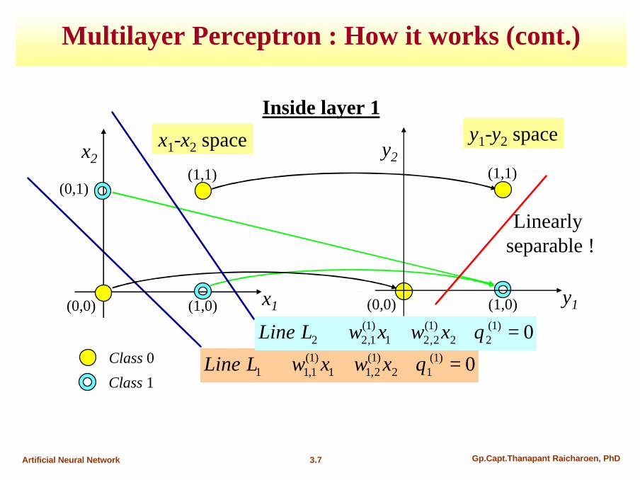
2-Layer case
(1) (1),
(1)
( )
( )
j j i i ji
j
y f w x
f h
θ= +
=
∑
ix
(1),j iw
(2) (2),
(2)
ˆ ( )
( )
k k j j kj
k
o f w y
f h
θ= +
=
∑
(2),k jw
ko
( ) weighted sum of input
of Node in Layer
nmh
m n
=

3.16 Gp.Capt.Thanapant Raicharoen, PhDArtificial Neural Network
2-Layer case2 2
(2) (2) 2,
(2) (1) (1) (2) 2, ,
ˆ( ) (2.1)
( ( )) (2.2)
( ( ( ) ))
k kk
k k j j kk j
k k j j i i j kj i
o o
o f w y
o f w f w x
ε
θ
θ θ
= −
= − +
= − ⋅ + +
∑
∑ ∑
∑ ∑ (2.3)k
∑
w(2)k,j
2(2)
(2),
ˆ 2 ( ) ( )k k k jk j
o o f h ywε∂ ′= − ⋅ − ⋅ ⋅
∂
The derivative of ε2 with respect to θ (2)k
2(2)
(2)ˆ 2 ( ) ( )k k k
k
o o f hε
θ∂ ′= − ⋅ − ⋅
∂
Backpropagation Algorithm (cont.)
The derivative of ε2 with respect to
3.17 Gp.Capt.Thanapant Raicharoen, PhDArtificial Neural Network
2-Layer case
The derivative of ε2 with respect to w(1)j,i
2(2) (2),(1) (1)
, ,
(2) (2) (2) (1) (1), , ,
(2) (2) (1),
ˆ 2 ( ) ( ( )
ˆ 2 ( ) ( ) ( )
ˆ 2 ( ) ( ) ( )
k k k j j kk jj i j i
k k k j j k k j j i i j ik j j
k k k k j j ik
o o f w yw w
o o f w y w f w x x
o o f h w f h x
εθ
θ θ
∂ ∂= − ⋅ − ⋅ +
∂ ∂
′ ′= − ⋅ − ⋅ + ⋅ ⋅ ⋅ + ⋅
′ ′= − ⋅ − ⋅ ⋅ ⋅ ⋅
∑ ∑
∑ ∑ ∑
∑
2 (2) (2) 2,
(2) (1) (1) (2) 2, ,
( ( )) (2.2)
( ( ( ) )) (2.3)
k k j j kk j
k k j j i i j kk j i
o f w y
o f w f w x
ε θ
θ θ
= − +
= − ⋅ + +
∑ ∑
∑ ∑ ∑
Backpropagation Algorithm (cont.)

3.18 Gp.Capt.Thanapant Raicharoen, PhDArtificial Neural Network
2(2) (2) (1)
,(1),
ˆ 2 ( ) ( ) ( )k k k k j j ikj i
o o f h w f h xwε∂ ′ ′= − ⋅ − ⋅ ⋅ ⋅ ⋅ ∂
∑
Taking the derivative of e2 with respect to w(1)j,i in order to adjust
the weight connecting the Node j of current layer (Layer 1) with Node i of Lower Layer (Layer 0)
Error from upper Node k
Derivative ofupper Node k
Weight betweenupper Node kand Node j of current layer
Derivative of Node j of current layer
Input fromlower Node i
This part is the back propagation of errorto Node j at current layer
Backpropagation Algorithm (cont.)

3.19 Gp.Capt.Thanapant Raicharoen, PhDArtificial Neural Network
derivative of ε2
with w(2)k,j
2(2)
2,
ˆ 2 ( ) ( )k k k jk j
o o f h ywε∂ ′= − ⋅ − ⋅ ⋅
∂
2(2) (2) (1)
,(1),
ˆ 2 ( ) ( ) ( )k k k k j j ikj i
o o f h w f h xwε∂ ′ ′= − ⋅ − ⋅ ⋅ ⋅ ⋅ ∂
∑derivative of e2
with w(1)j,i
Error at current node Input from lower node
Derivative of current node
Backpropagation Algorithm (cont.)

3.20 Gp.Capt.Thanapant Raicharoen, PhDArtificial Neural Network
2( ) ( ) ( ) ( 1), ( )
,
2( ) ( ) ( )
( )
( )
( )
n n n nj i j j in
j i
n n nj j jn
j
w f h xw
f h
εα α
εθ α α
θ
−∂ ′∆ = − ⋅ = ⋅∆ ⋅ ⋅∂
∂ ′∆ = − ⋅ = ⋅∆ ⋅∂
Updating Weights : Gradient Descent Method
Updating weights and bias
( ) ( ) ( ), , ,
( ) ( ) ( )
( ) ( )
( ) ( )
n n nj i j i j i
n n nj j j
w new w old w
new oldθ θ θ
= + ∆
= + ∆
3.21 Gp.Capt.Thanapant Raicharoen, PhDArtificial Neural Network
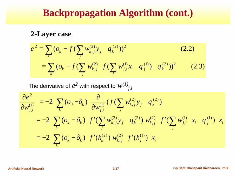
Adjusting Weights for a Nonlinear Function (Unit)
xexf β21
1)( −+
=
calculation f ? , in case of nonlinear (function) unit
))(1()(2)( xfxfxf −⋅⋅=′ β
1. Sigmoid function
We get
2. Function tanh(x) )tanh()( xxf β=
We get ))(1()( 2xfxf −⋅=′ β
Special case of f ?It’s easy to calculate f ´

3.22 Gp.Capt.Thanapant Raicharoen, PhDArtificial Neural Network
Backpropagation Calculation DemonstrationBackpropagation Calculation Demonstration
3.23 Gp.Capt.Thanapant Raicharoen, PhDArtificial Neural Network
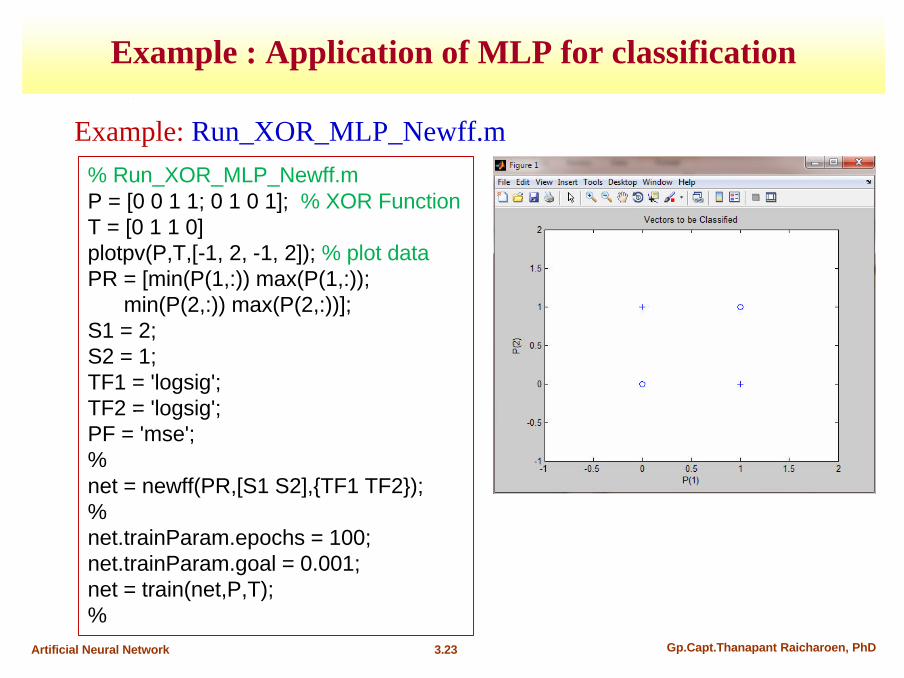
Example : Application of MLP for classification
Example: Run_XOR_MLP_Newff.m% Run_XOR_MLP_Newff.mP = [0 0 1 1; 0 1 0 1]; % XOR FunctionT = [0 1 1 0]plotpv(P,T,[-1, 2, -1, 2]); % plot dataPR = [min(P(1,:)) max(P(1,:));
min(P(2,:)) max(P(2,:))]; S1 = 2; S2 = 1; TF1 = 'logsig';TF2 = 'logsig';PF = 'mse';%net = newff(PR,[S1 S2],{TF1 TF2});%net.trainParam.epochs = 100;net.trainParam.goal = 0.001;net = train(net,P,T);%

3.24 Gp.Capt.Thanapant Raicharoen, PhDArtificial Neural Network
-3 -2 -1 0 1 2 3-3
-2
-1
0
1
2
Class 1Class 0
Example : Application of MLP for classification
x = randn([2 200]);
o = (x(1,:).^2+x(2,:).^2)<1;
Example: Run_MLP_Random.mMatlab command : Create training data
Input pattern x1 and x2 generated from random numbers
Desired output o:if (x1,x2) lies in a circle of radius 1centered at the origin then
o = 1else
o = 0
x2
x1

3.25 Gp.Capt.Thanapant Raicharoen, PhDArtificial Neural Network
PR = [min(x(1,:)) max(x(1,:));
min(x(2,:)) max(x(2,:))];
S1 = 10;
S2 = 1;
TF1 = 'logsig';
TF2 = 'logsig';
BTF = 'traingd';
BLF = 'learngd';
PF = 'mse';
net = newff(PR,[S1 S2],{TF1 TF2},BTF,BLF,PF);
Matlab command : Create a 2-layer network
Range of inputs
No. of nodes in Layers 1 and 2
Activation functions of Layers 1 and 2
Training functionLearning function
Cost function
Command for creating the network
Example : Application of MLP for classification (cont.)

3.26 Gp.Capt.Thanapant Raicharoen, PhDArtificial Neural Network
Matlab command : Train the network
net.trainParam.epochs = 2000;
net.trainParam.goal = 0.002;
net = train(net,x,o);
y = sim(net,x);
netout = y>0.5;
No. of training roundsMaximum desired errorTraining command
Compute network outputs (continuous)Convert to binary outputs
Example : Application of MLP for classification (cont.)
3.27 Gp.Capt.Thanapant Raicharoen, PhDArtificial Neural Network
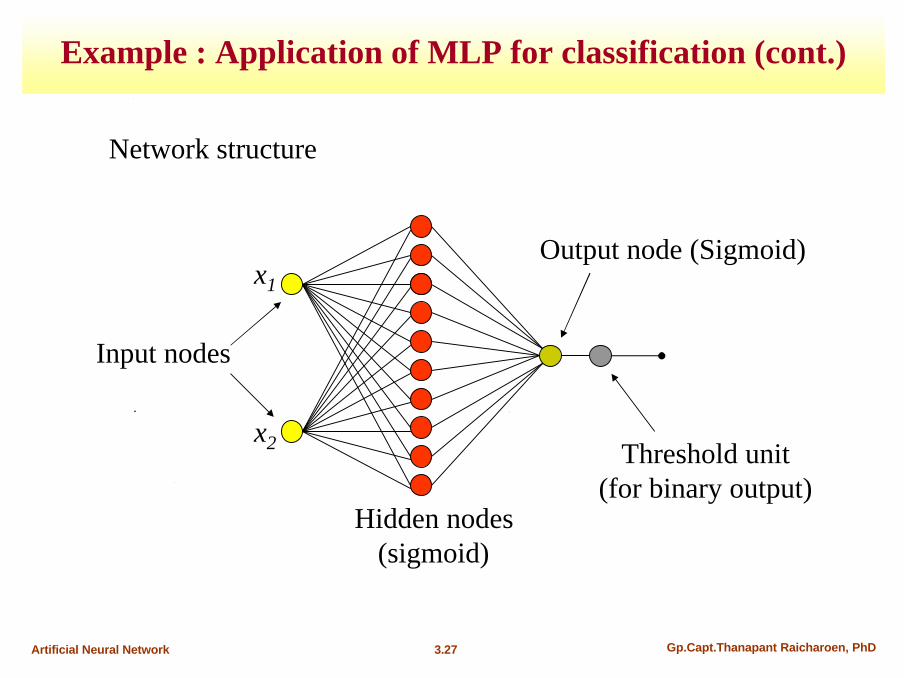
Network structure
x2
x1
Hidden nodes(sigmoid)
Output node (Sigmoid)
Input nodes
Threshold unit(for binary output)
Example : Application of MLP for classification (cont.)
3.28 Gp.Capt.Thanapant Raicharoen, PhDArtificial Neural Network
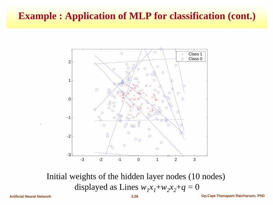
Initial weights of the hidden layer nodes (10 nodes) displayed as Lines w1x1+w2x2+θ = 0
-3 -2 -1 0 1 2 3-3
-2
-1
0
1
2
Class 1Class 0
Example : Application of MLP for classification (cont.)

3.29 Gp.Capt.Thanapant Raicharoen, PhDArtificial Neural Network MSE vs training epochs
Training algorithm: Gradient descent method
0 0.5 1 1.5 2
x 104
10-3
10-2
10-1
100 Performance is 0.151511, Goal is 0.002
20000 Epochs
Trai
ning
-Blu
e G
oal-B
lack
Example : Application of MLP for classification (cont.)

3.30 Gp.Capt.Thanapant Raicharoen, PhDArtificial Neural Network
Results obtained using the Gradient descent method
Classification Error : 40/200
-3 -2 -1 0 1 2 3-3
-2
-1
0
1
2
Class 1Class 0
Example : Application of MLP for classification (cont.)

3.31 Gp.Capt.Thanapant Raicharoen, PhDArtificial Neural Network MSE vs training epochs (success with in only 10 epochs!)
Training algorithm: Levenberg-Marquardt Backpropagation
0 2 4 6 8 1010
-3
10-2
10-1
100 Performance is 0.00172594, Goal is 0.002
10 Epochs
Trai
ning
-Blu
e G
oal-B
lack
Example : Application of MLP for classification (cont.)
3.32 Gp.Capt.Thanapant Raicharoen, PhDArtificial Neural Network
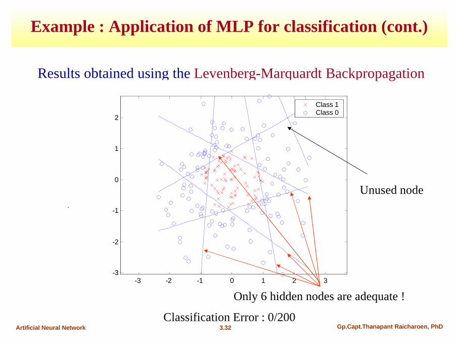
Results obtained using the Levenberg-Marquardt Backpropagation
Classification Error : 0/200
-3 -2 -1 0 1 2 3-3
-2
-1
0
1
2
Class 1Class 0
Unused node
Only 6 hidden nodes are adequate !
Example : Application of MLP for classification (cont.)

3.33 Gp.Capt.Thanapant Raicharoen, PhDArtificial Neural Network
Summary: MLP for Classification Problem
- Each lower layer (hidden) Nodes of Neural Network createa local boundary decision.
- The upper layer Nodes of Neural Network combine all localboundary decisions to a global boundary decision.
Example : Application of MLP for classification (cont.)

3.34 Gp.Capt.Thanapant Raicharoen, PhDArtificial Neural Network
PR = [min(x) max(x)]
S1 = 6;
S2 = 1;
TF1 = 'logsig';
TF2 = 'purelin';
BTF = 'trainlm';
BLF = 'learngd';
PF = 'mse';
net = newff(PR,[S1 S2],{TF1 TF2},BTF,BLF,PF);
Example: Run_MLP_SinFunction.mMatlab command : Create a 2-layer network
Range of inputs
No. of nodes in Layers 1 and 2
Activation functions of Layers 1 and 2
Training functionLearning function
Cost function
Command for creating the network
Example: Application of MLP for function approximation
3.35 Gp.Capt.Thanapant Raicharoen, PhDArtificial Neural Network
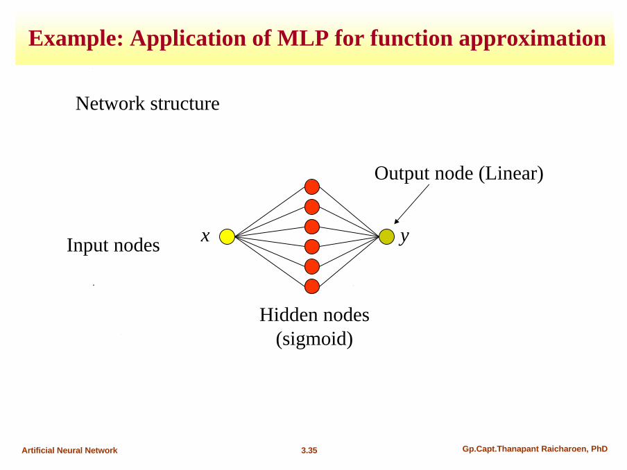
Network structure
Hidden nodes(sigmoid)
Output node (Linear)
Input nodes x y
Example: Application of MLP for function approximation

3.36 Gp.Capt.Thanapant Raicharoen, PhDArtificial Neural Network
Example: Run_MLP_SinFunction.m
Example: Application of MLP for function approximation
% Run_MLP_SinFunction.mp=0:0.25:5;t = sin(p);figure;plot(p,t,'+b'); axis([-0.5 5.5 -1.5 1.5 ]); %net = newff([0 10],[6,1],{'logsig','purelin'},'trainlm');%net.trainParam.epochs = 50; net.trainParam.goal = 0.01;net = train(net,p,t);%a = sim(net,p);hold on;plot(p,a,'.r');%…

3.37 Gp.Capt.Thanapant Raicharoen, PhDArtificial Neural Network
PR = [min(x) max(x)]
S1 = 3;
S2 = 1;
TF1 = 'logsig';
TF2 = 'purelin';
BTF = 'trainlm';
BLF = 'learngd';
PF = 'mse';
net = newff(PR,[S1 S2],{TF1TF2},BTF,BLF,PF);
Matlab command : Create a 2-layer network
Range of inputs
No. of nodes in Layers 1 and 2
Activation functions of Layers 1 and 2
Training functionLearning function
Cost function
Command for creating the network
Example: Application of MLP for function approximation

3.38 Gp.Capt.Thanapant Raicharoen, PhDArtificial Neural Network
Example: Application of MLP for function approximation
0 0.5 1 1.5 2 2.5 3 3.5 40
0.2
0.4
0.6
0.8
1
1.2
1.4
1.6
1.8
Input x
Out
put y
Function to be approximated
x = 0:0.01:4;
y = (sin(2*pi*x)+1).*exp(-x.^2);

3.39 Gp.Capt.Thanapant Raicharoen, PhDArtificial Neural Network
0 0.5 1 1.5 2 2.5 3 3.5 40
0.2
0.4
0.6
0.8
1
1.2
1.4
1.6
1.8
2Desired outputNetwork output
Networkstructure
No. of hidden nodes is too small !
Function approximated using the network
Example: Application of MLP for function approximation

3.40 Gp.Capt.Thanapant Raicharoen, PhDArtificial Neural Network
PR = [min(x) max(x)]
S1 = 5;
S2 = 1;
TF1 = 'radbas';
TF2 = 'purelin';
BTF = 'trainlm';
BLF = 'learngd';
PF = 'mse';
net = newff(PR,[S1 S2],{TF1TF2},BTF,BLF,PF);
Matlab command : Create a 2-layer network
Range of inputs
No. of nodes in Layers 1 and 2
Activation functions of Layers 1 and 2
Training functionLearning function
Cost function
Command for creating the network
Example: Application of MLP for function approximation
3.41 Gp.Capt.Thanapant Raicharoen, PhDArtificial Neural Network
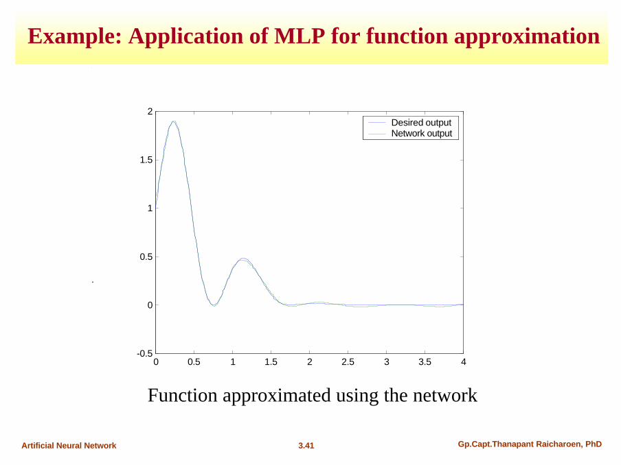
Function approximated using the network
0 0.5 1 1.5 2 2.5 3 3.5 4-0.5
0
0.5
1
1.5
2Desired outputNetwork output
Example: Application of MLP for function approximation
3.42 Gp.Capt.Thanapant Raicharoen, PhDArtificial Neural Network
Example: Application of MLP for function approximation
Summary: MLP for Function Approximation Problem
- Each lower layer (hidden) nodes of Neural Network createa local (short) approximated function.
- The upper layer Nodes of Neural Network combine all local approximated function to global approximated function coverall input range.

3.43 Gp.Capt.Thanapant Raicharoen, PhDArtificial Neural Network
Summary
§ Backpropagation can train multilayer feed-forward networks with differentiable transfer functions to perform function approximation, pattern association, and pattern classification. § The term backpropagation refers to the process by which derivatives of network error, with respect to network weights and biases, can be computed.§ The number of inputs and outputs to the network are constrained by the problem. However, the number of layersbetween network inputs and the output layer and the sizes of the layers are up to the designer. § The two-layer sigmoid/linear network can represent any functional relationship between inputs and outputs if the sigmoid layer has enough neurons.
3.44 Gp.Capt.Thanapant Raicharoen, PhDArtificial Neural Network
Programming in MATLAB ExerciseProgramming in MATLAB Exercise
n Exercise:
1. Write MATLAB to solve the question 1 in Exercise 4.
2. Write MATLAB to solve the question 2 in Exercise 4.