Programming for FPGAs

419© Intel Corporation 2021 J. Reinders et al., Data Parallel C++, https://doi.org/10.1007/978-1-4842-5574-2_17

CHAPTER 17

Programming for FPGAs

FPGAemulator pi

pes

Kernel-based programming originally became popular as a way to access

GPUs. Since it has now been generalized across many types of accelerators,

it is important to understand how our style of programming affects the

mapping of code to an FPGA as well.

Field Programmable Gate Arrays (FPGAs) are unfamiliar to the majority

of software developers, in part because most desktop computers don’t

include an FPGA alongside the typical CPU and GPU. But FPGAs are worth

knowing about because they offer advantages in many applications. The same

questions need to be asked as we would of other accelerators, such as “When

should I use an FPGA?”, “What parts of my applications should be offloaded to

FPGA?”, and “How do I write code that performs well on an FPGA?”

This chapter gives us the knowledge to start answering those

questions, at least to the point where we can decide whether an FPGA

is interesting for our applications, and to know which constructs are

commonly used to achieve performance. This chapter is the launching

https://doi.org/10.1007/978-1-4842-5574-2_17#DOI

420

point from which we can then read vendor documentation to fill in details

for specific products and toolchains. We begin with an overview of how

programs can map to spatial architectures such as FPGAs, followed by

discussion of some properties that make FPGAs a good choice as an

accelerator, and we finish by introducing the programming constructs

used to achieve performance.

The “How to Think About FPGAs” section in this chapter is applicable

to thinking about any FPGA. SYCL allows vendors to specify devices

beyond CPUs and GPUs, but does not specifically say how to support

an FPGA. The specific vendor support for FPGAs is currently unique to

DPC++, namely, FPGA selectors and pipes. FPGA selectors and pipes are

the only DPC++ extensions used in this chapter. It is hoped that vendors

will converge on similar or compatible means of supporting FPGAs, and

this is encouraged by DPC++ as an open source project.

Performance CaveatsAs with any processor or accelerator, FPGA devices differ from vendor to

vendor or even from product generation to product generation; therefore,

best practices for one device may not be best practices for a different

device. The advice in this chapter is likely to benefit many FPGA devices,

both now and in the future, however…

…to achieve optimal performance for a particular FPGA, always consult the vendor’s documentation!

How to Think About FPGAsFPGAs are commonly classified as a spatial architecture. They benefit from

very different coding styles and forms of parallelism than devices that use

an Instruction Set Architecture (ISA), including CPUs and GPUs, which are

ChAPter 17 ProGrAmminG For FPGAs

421

more familiar to most people. To get started forming an understanding of

FPGAs, we’ll briefly cover some ideas from ISA-based accelerators, so that

we can highlight key differences.

For our purposes, an ISA-based accelerator is one where the device

can execute many different instructions, one or a few at a time. The

instructions are usually relatively primitive such as “load from memory at

address A” or “add the following numbers.” A chain of operations is strung

together to form a program, and the processor conceptually executes one

instruction after the other.

In an ISA-based accelerator, a single region of a chip (or the entire

chip) executes a different instruction from the program in each clock cycle.

The instructions execute on a fixed hardware architecture that can run

different instructions at different times, such as shown in Figure 17-1.

For example, the memory load unit feeding an addition is probably

the same memory load unit used to feed a subtraction. Similarly, the

same arithmetic unit is probably used to execute both the addition and

subtraction instructions. Hardware on the chip is reused by different

instructions as the program executes over time.

Memory Load/Store

Simple SA-based Accelerator

Arithmetic Unit (+,-,*)

ProgramCounter

InstructionFetch/Decode

Registers

MUX MUX

Figure 17-1. Simple ISA-based (temporal) processing: Reuses hardware (regions) over time


422

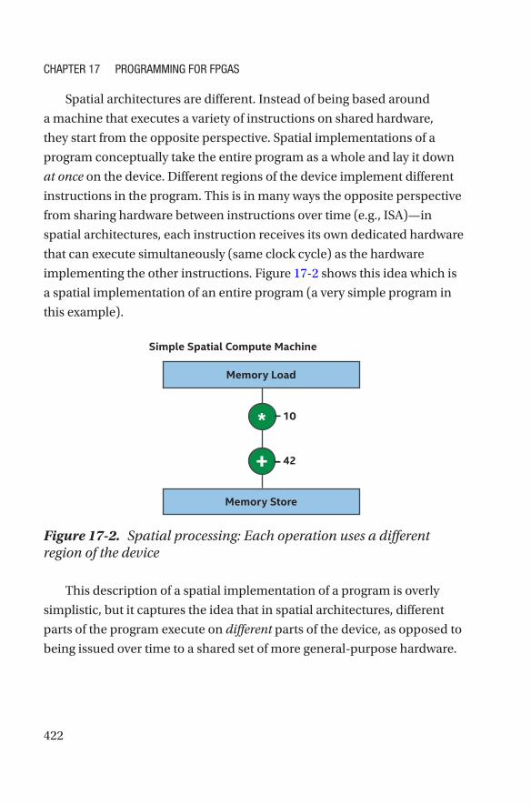
Spatial architectures are different. Instead of being based around

a machine that executes a variety of instructions on shared hardware,

they start from the opposite perspective. Spatial implementations of a

program conceptually take the entire program as a whole and lay it down

at once on the device. Different regions of the device implement different

instructions in the program. This is in many ways the opposite perspective

from sharing hardware between instructions over time (e.g., ISA)—in

spatial architectures, each instruction receives its own dedicated hardware

that can execute simultaneously (same clock cycle) as the hardware

implementing the other instructions. Figure 17-2 shows this idea which is

a spatial implementation of an entire program (a very simple program in

this example).

Figure 17-2. Spatial processing: Each operation uses a different region of the device

This description of a spatial implementation of a program is overly

simplistic, but it captures the idea that in spatial architectures, different

parts of the program execute on different parts of the device, as opposed to

being issued over time to a shared set of more general-purpose hardware.


423

With different regions of an FPGA programmed to perform distinct

operations, some of the hardware typically associated with ISA-based

accelerators is unnecessary. For example, Figure 17-2 shows that we no

longer need an instruction fetch or decode unit, program counter, or register

file. Instead of storing data for future instructions in a register file, spatial

architectures connect the output of one instruction to the input of the next,

which is why spatial architectures are often called data flow architectures.

A few obvious questions arise from the mapping to FPGA that we’ve

introduced. First, since each instruction in the program occupies some

percentage of the spatial area of the device, what happens if the program

requires more than 100% of the area? Some solutions provide resource

sharing mechanisms to enable larger programs to fit at a performance

cost, but FPGAs do have the concept of a program fitting. This is both an

advantage and a disadvantage:

• The benefit: If a program uses most of the area on

the FPGA and there is sufficient work to keep all of

the hardware busy every clock cycle, then executing

a program on the device can be incredibly efficient

because of the extreme parallelism. More general

architectures may have significant unused hardware

per clock cycle, whereas with an FPGA, the use of

area can be perfectly tailored to a specific application

without waste. This customization can allow

applications to run faster through massive parallelism,

usually with compelling energy efficiency.

• The downside: Large programs may have to be tuned

and restructured to fit on a device. Resource sharing

features of compilers can help to address this, but

usually with some degradation in performance that

reduces the benefit of using an FPGA. ISA-based

accelerators are very efficient resource sharing


424

implementations—FPGAs prove most valuable

for compute primarily when an application can be

architected to utilize most of the available area.

Taken to the extreme, resource sharing solutions on an FPGA lead

to an architecture that looks like an ISA-based accelerator, but that is

built in reconfigurable logic instead being optimized in fixed silicon. The

reconfigurable logic leads to overhead relative to a fixed silicon design—

therefore, FPGAs are not typically chosen as ways to implement ISAs.

FPGAs are of prime benefit when an application is able to utilize the

resources to implement efficient data flow algorithms, which we cover in

the coming sections.

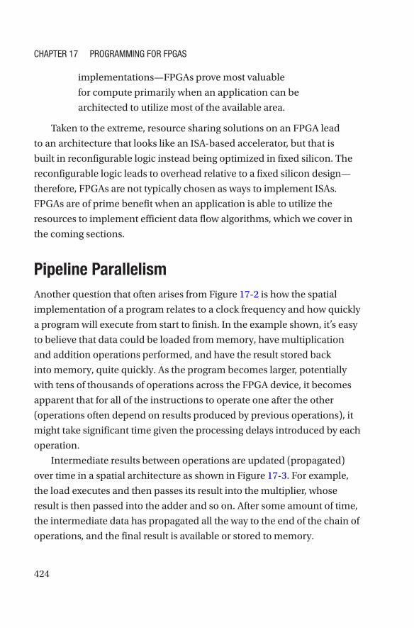
Pipeline ParallelismAnother question that often arises from Figure 17-2 is how the spatial

implementation of a program relates to a clock frequency and how quickly

a program will execute from start to finish. In the example shown, it’s easy

to believe that data could be loaded from memory, have multiplication

and addition operations performed, and have the result stored back

into memory, quite quickly. As the program becomes larger, potentially

with tens of thousands of operations across the FPGA device, it becomes

apparent that for all of the instructions to operate one after the other

(operations often depend on results produced by previous operations), it

might take significant time given the processing delays introduced by each

operation.

Intermediate results between operations are updated (propagated)

over time in a spatial architecture as shown in Figure 17-3. For example,

the load executes and then passes its result into the multiplier, whose

result is then passed into the adder and so on. After some amount of time,

the intermediate data has propagated all the way to the end of the chain of

operations, and the final result is available or stored to memory.


425

A spatial implementation as shown in Figure 17-3 is quite inefficient,

because most of the hardware is only doing useful work a small percentage

of the time. Most of the time, an operation such as the multiply is

either waiting for new data from the load or holding its output so that

operations later in the chain can use its result. Most spatial compilers and

implementations address this inefficiency by pipelining, which means that

execution of a single program is spread across many clock cycles. This is

achieved by inserting registers (a data storage primitive in the hardware)

between some operations, where each register holds a binary value for the

duration of a clock cycle. By holding the result of an operation’s output so

that the next operation in the chain can see and operate on that held value,

the previous operation is free to work on a different computation without

impacting the input to following operations.

The goal of algorithmic pipelining is to keep every operation

(hardware unit) busy every clock cycle. Figure 17-4 shows a pipelined

implementation of the previous simple example. Keep in mind that the

compiler does all of the pipelining and balancing for us! We cover this

topic so that we can understand how to fill the pipeline with work in the

coming sections, not because we need to worry about manually pipelining

anything in our code.

Figure 17-3. Propagation time of a naïve spatial compute implementation


426

When a spatial implementation is pipelined, it becomes extremely

efficient in the same way as a factory assembly line. Each pipeline stage

performs only a small amount of the overall work, but it does so quickly

and then begins to work on the next unit of work immediately afterward.

It takes many clock cycles for a single computation to be processed by the

pipeline, from start to finish, but the pipeline can compute many different

instances of the computation on different data simultaneously.

When enough work starts executing in the pipeline, over enough

consecutive clock cycles, then every single pipeline stage and therefore

operation in the program can perform useful work during every

clock cycle, meaning that the entire spatial device performs work

simultaneously. This is one of the powers of spatial architectures—the

entire device can execute work in parallel, all of the time. We call this

pipeline parallelism.

Pipeline parallelism is the primary form of parallelism exploited on FPGAs to achieve performance.

*

+

Figure 17-4. Pipelining of a computation: Stages execute in parallel


427

PIPELINING IS AUTOMATIC

in the intel implementation of DPC++ for FPGAs, and in other high-level

programming solutions for FPGAs, the pipelining of an algorithm is performed

automatically by the compiler. it is useful to roughly understand the

implementation on spatial architectures, as described in this section, because

then it becomes easier to structure applications to take advantage of the

pipeline parallelism. it should be made clear that pipeline register insertion and

balancing is performed by the compiler and not manually by developers.

Real programs and algorithms often have control flow (e.g., if/else

structures) that leaves some parts of the program inactive a certain

percentage of the clock cycles. FPGA compilers typically combine

hardware from both sides of a branch, where possible, to minimize

wasted spatial area and to maximize compute efficiency during control

flow divergence. This makes control flow divergence much less expensive

and less of a development concern than on other, especially vectorized

architectures.

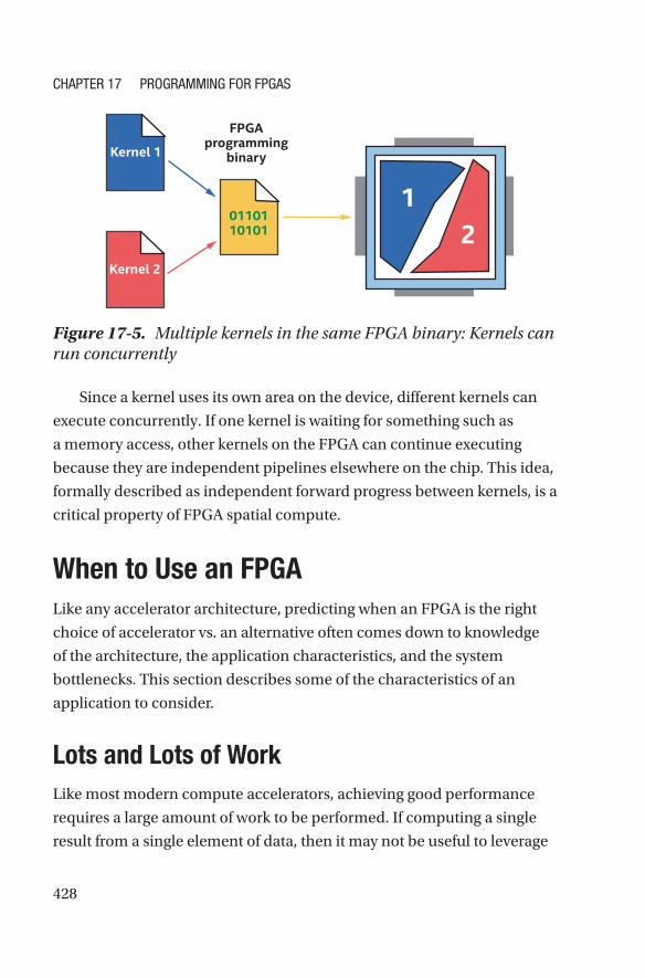
Kernels Consume Chip “Area”In existing implementations, each kernel in a DPC++ application generates

a spatial pipeline that consumes some resources of the FPGA (we can think

about this as space or area on the device), which is conceptually shown in

Figure 17-5.


428

Since a kernel uses its own area on the device, different kernels can

execute concurrently. If one kernel is waiting for something such as

a memory access, other kernels on the FPGA can continue executing

because they are independent pipelines elsewhere on the chip. This idea,

formally described as independent forward progress between kernels, is a

critical property of FPGA spatial compute.

When to Use an FPGALike any accelerator architecture, predicting when an FPGA is the right

choice of accelerator vs. an alternative often comes down to knowledge

of the architecture, the application characteristics, and the system

bottlenecks. This section describes some of the characteristics of an

application to consider.

Lots and Lots of WorkLike most modern compute accelerators, achieving good performance

requires a large amount of work to be performed. If computing a single

result from a single element of data, then it may not be useful to leverage

Figure 17-5. Multiple kernels in the same FPGA binary: Kernels can run concurrently


429

an accelerator at all (of any kind). This is no different with FPGAs. Knowing

that FPGA compilers leverage pipeline parallelism makes this more

apparent. A pipelined implementation of an algorithm has many stages,

often thousands or more, each of which should have different work within

it in any clock cycle. If there isn’t enough work to occupy most of the

pipeline stages most of the time, then efficiency will be low. We’ll call the

average utilization of pipeline stages over time occupancy of the pipeline.

This is different from the definition of occupancy used when optimizing

other architectures such as GPUs!

There are multiple ways to generate work on an FPGA to fill the

pipeline stages, which we’ll cover in coming sections.

Custom Operations or Operation WidthsFPGAs were originally designed to perform efficient integer and bitwise

operations and to act as glue logic that could adapt interfaces of other

chips to work with each other. Although FPGAs have evolved into

computational powerhouses instead of just glue logic solutions, they are

still very efficient at bitwise operations, integer math operations on custom

data widths or types, and operations on arbitrary bit fields in packet

headers.

The fine-grained architecture of an FPGA, described at the end of

this chapter, means that novel and arbitrary data types can be efficiently

implemented. For example, if we need a 33-bit integer multiplier or a

129-bit adder, FPGAs can provide these custom operations with great

efficiency. Because of this flexibility, FPGAs are commonly employed in

rapidly evolving domains, such as recently in machine learning, where the

data widths and operations have been changing faster than can be built

into ASICs.


430

Scalar Data FlowAn important aspect of FPGA spatial pipelines, apparent from Figure 17-4,

is that the intermediate data between operations not only stays on-chip

(is not stored to external memory), but that intermediate data between

each pipeline stage has dedicated storage registers. FPGA parallelism

comes from pipelining of computation such that many operations are

being executed concurrently, each at a different stage of the pipeline. This

is different from vector architectures where multiple computations are

executed as lanes of a shared vector instruction.

The scalar nature of the parallelism in a spatial pipeline is important for

many applications, because it still applies even with tight data dependences

across the units of work. These data dependences can be handled without

loss of performance, as we will discuss later in this chapter when talking about

loop-carried dependences. The result is that spatial pipelines, and therefore

FPGAs, are compelling for algorithms where data dependences across units of

work (such as work-items) can’t be broken and fine-grained communication

must occur. Many optimization techniques for other accelerators focus

on breaking these dependences though various techniques or managing

communication at controlled scales through features such as sub-groups.

FPGAs can instead perform well with communication from tight dependences

and should be considered for classes of algorithms where such patterns exist.

LOOPS ARE FINE!

A common misconception on data flow architectures is that loops with either

fixed or dynamic iteration counts lead to poor data flow performance, because

they aren’t simple feed-forward pipelines. At least with the intel DPC++ and

FPGA toolchains, this is not true. Loop iterations can instead be a good way to

produce high occupancy within the pipeline, and the compilers are built around

the concept of allowing multiple loop iterations to execute in an overlapped

way. Loops provide an easy mechanism to keep the pipeline busy with work!


431

Low Latency and Rich ConnectivityMore conventional uses of FPGAs which take advantage of the rich input

and output transceivers on the devices apply equally well for developers

using DPC++. For example, as shown in Figure 17-6, some FPGA

accelerator cards have network interfaces that make it possible to stream

data directly into the device, process it, and then stream the result directly

back to the network. Such systems are often sought when processing

latency needs to be minimized and where processing through operating

system network stacks is too slow or needs to be offloaded.

Figure 17-6. Low-latency I/O streaming: FPGA connects network data and computation tightly

The opportunities are almost limitless when considering direct input/

output through FPGA transceivers, but the options do come down to

what is available on the circuit board that forms an accelerator. Because

of the dependence on a specific accelerator card and variety of such uses,

aside from describing the pipe language constructs in a coming section,

this chapter doesn’t dive into these applications. We should instead read

the vendor documentation associated with a specific accelerator card or

search for an accelerator card that matches our specific interface needs.


432

Customized Memory SystemsMemory systems on an FPGA, such as function private memory or work-

group local memory, are built out of small blocks of on-chip memory. This

is important because each memory system is custom built for the specific

portion of an algorithm or kernel using it. FPGAs have significant on-chip

memory bandwidth, and combined with the formation of custom memory

systems, they can perform very well on applications that have atypical

memory access patterns and structures. Figure 17-7 shows some of the

optimizations that can be performed by the compiler when a memory

system is implemented on an FPGA.

Figure 17-7. FPGA memory systems are customized by the compiler for our specific code

Other architectures such as GPUs have fixed memory structures that

are easy to reason about by experienced developers, but that can also be

hard to optimize around in many cases. Many optimizations on other

accelerators are focused around memory pattern modification to avoid

bank conflicts, for example. If we have algorithms that would benefit from

a custom memory structure, such as a different number of access ports

per bank or an unusual number of banks, then FPGAs can offer immediate

advantages. Conceptually, the difference is between writing code to use a

fixed memory system efficiently (most other accelerators) and having the

memory system custom designed by the compiler to be efficient with our

specific code (FPGA).


433

Running on an FPGAThere are two steps to run a kernel on an FPGA (as with any ahead-of-time

compilation accelerator):

1. Compiling the source to a binary which can be run

on our hardware of interest

2. Selecting the correct accelerator that we are

interested in at runtime

To compile kernels so that they can run on FPGA hardware, we can use

the command line:

dpcpp -fintelfpga my_source_code.cpp -Xshardware

This command tells the compiler to turn all kernels in my_source_

code.cpp into binaries that can run on an Intel FPGA accelerator and then

to package them within the host binary that is generated. When we execute

the host binary (e.g., by running ./a.out on Linux), the runtime will

automatically program any attached FPGA as required, before executing

the submitted kernels, as shown in Figure 17-8.


434

FPGA programming binaries are embedded within the compiled DPC++ executable that we run on the host. the FPGA is automatically configured behind the scenes for us.

When we run a host program and submit the first kernel for execution on an FPGA, there might be a slight delay before the kernel begins executing, while the FPGA is programmed. resubmitting kernels for additional executions won’t see the same delay because the kernel is already programmed to the device and ready to run.

Selection of an FPGA device at runtime was covered in Chapter 2. We

need to tell the host program where we want kernels to run because there

are typically multiple accelerator options available, such as a CPU and

GPU, in addition to the FPGA. To quickly recap one method to select an

FPGA during program execution, we can use code like that in Figure 17-9.

FPGAprogramming

binary

Programming is automatic! The DPC++ runtime programs the FPGA device behind the scenes when needed, before a kernel runs on it.

Fat binary

FPGA binary

Host binary

Kernel 1

Kernel 2

0110110101

0110110101

0110110101

12

Figure 17-8. FPGA programmed automatically at runtime


https://doi.org/10.1007/978-1-4842-5574-2_2

435

Compile TimesRumors abound that compiling designs for an FPGA can take a long time, much

longer than compiling for ISA-based accelerators. The rumors are true! The end

of this chapter overviews the fine-grained architectural elements of an FPGA

that lead to both the advantages of an FPGA and the computationally intensive

compilation (place-and-route optimizations) that can take hours in some cases.

The compile time from source code to FPGA hardware execution

is long enough that we don’t want to develop and iterate on our code

exclusively in hardware. FPGA development flows offer several stages

that minimize the number of hardware compilations, to make us

productive despite the hardware compile times. Figure 17-10 shows

the typical stages, where most of our time is spent on the early steps

that provide fast turnaround and rapid iteration.

#include <CL/sycl.hpp>#include <CL/sycl/intel/fpga_extensions.hpp> // For fpga_selectorusing namespace sycl;

void say_device (const queue& Q) {std::cout << "Device : "

<< Q.get_device().get_info<info::device::name>() << "\n";

}

int main() {queue Q{ INTEL::fpga_selector{} };say_device(Q);

Q.submit([&](handler &h){h.parallel_for(1024, [=](auto idx) {

// ...});

});

return 0;}

Figure 17-9. Choosing an FPGA device at runtime using the fpga_selector


436

Emulation and static reports from the compiler are the cornerstones

of FPGA code development in DPC++. The emulator acts as if it was

an FPGA, including supporting relevant extensions and emulating the

execution model, but runs on the host processor. Compilation time

is therefore the same as we would expect from compilation to a CPU

device, although we won’t see the performance boost that we would from

execution on actual FPGA hardware. The emulator is great for establishing

and testing functional correctness in an application.

Static reports, like emulation, are generated quickly by the toolchain.

They report on the FPGA structures created by the compiler and on

bottlenecks identified by the compiler. Both of these can be used to predict

whether our design will achieve good performance when run on FPGA

hardware and are used to optimize our code. Please read the vendor’s

documentation for information on the reports, which are often improved

from release to release of a toolchain (see documentation for the latest

and greatest features!). Extensive documentation is provided by vendors

Figure 17-10. Most verification and optimization occurs prior to lengthy hardware compilation


437

on how to interpret and optimize based on the reports. This information

would be the topic of another book, so we can’t dive into details in this

single chapter.

The FPGA Emulator

Emulation is primarily used to functionally debug our application, to make

sure that it behaves as expected and produces correct results. There is no

reason to do this level of development on actual FPGA hardware where

compile times are longer. The emulation flow is activated by removing

the -Xshardware flag from the dpcpp compilation command and at the

same time using the INTEL::fpga_emulator_selector instead of the

INTEL::fpga_selector in our host code. We would compile using a

command like

dpcpp -fintelfpga my_source_code.cpp

Simultaneously, we would choose the FPGA emulator at runtime

using code such as in Figure 17-11. By using fpga_emulator_selector,

which uses the host processor to emulate an FPGA, we maintain a rapid

development and debugging process before we have to commit to the

lengthier compile for actual FPGA hardware.


438

If we are switching between hardware and the emulator frequently, it

can make sense to use a macro within our program to flip between device

selectors from the command line. Check the vendor’s documentation and

online FPGA DPC++ code examples for examples of this, if needed.

FPGA Hardware Compilation Occurs “Ahead-of-Time”

The Full Compile and Hardware Profiling stage in Figure 17-10 is an ahead-

of- time compile in SYCL terminology. This means that the compilation of

the kernel to a device binary occurs when we initially compile our program

and not when the program is submitted to a device to be run. On an FPGA,

this is particularly important because

#include <CL/sycl.hpp>

#include <CL/sycl/intel/fpga_extensions.hpp> // For fpga_selectorusing namespace sycl;

void say_device (const queue& Q) {std::cout << "Device : "<< Q.get_device().get_info<info::device::name>() << "\n";

}

int main() {queue Q{ INTEL::fpga_emulator_selector{} };say_device(Q);

Q.submit([&](handler &h){h.parallel_for(1024, [=](auto idx) {

// ...});

});

return 0;}

Figure 17-11. Using fpga_emulator_selector for rapid development and debugging


439

1. Compilation takes a length of time that we

don’t normally want to incur when running an

application.

2. DPC++ programs may be executed on systems

that don’t have a capable host processor. The

compilation process to an FPGA binary benefits

from a fast processor with a good amount of

attached memory. Ahead- of- time compilation lets

us easily choose where the compile occurs, rather

than having it run on systems where the program is

deployed.

A LOT HAPPENS BEHIND THE SCENES WITH DPC++ ON AN FPGA!

Conventional FPGA design (not using a high-level language) can be very

complicated. there are many steps beyond just writing our kernel, such

as building and configuring the interfaces that communicate with off-chip

memories and closing timing by inserting registers needed to make the

compiled design run fast enough to communicate with certain peripherals.

DPC++ solves all of this for us, so that we don’t need to know anything about

the details of conventional FPGA design to achieve working applications!

the tooling treats our kernels as code to optimize and make efficient on the

device and then automatically handles all of the details of talking to off-chip

peripherals, closing timing, and setting up drivers for us.

Achieving peak performance on an FPGA still requires detailed knowledge of

the architecture, just like any other accelerator, but the steps to move from

code to a working design are much simpler and more productive with DPC++

than in traditional FPGA flows.


440

Writing Kernels for FPGAsOnce we have decided to use an FPGA for our application or even just

decided to try one out, having an idea of how to write code to see good

performance is important. This section describes topics that highlight

important concepts and covers a few topics that often cause confusion, to

make getting started faster.

Exposing ParallelismWe have already looked at how pipeline parallelism is used to efficiently

perform work on an FPGA. Another simple pipeline example is shown in

Figure 17- 12.

Figure 17-12. Simple pipeline with five stages: Six clock cycles to process an element of data


441

In this pipeline, there are five stages. Data moves from one stage to the

next once per clock cycle, so in this very simple example, it takes six clock

cycles from when data enters into stage 1 until it exits from stage 5.

A major goal of pipelining is to enable multiple elements of data to be

processed at different stages of the pipeline, simultaneously. To be sure

that this is clear, Figure 17-13 shows a pipeline where there is not enough

work (only one element of data in this case), which causes each pipeline

stage to be unused during most of the clock cycles. This is an inefficient

use of the FPGA resources because most of the hardware is idle most of

the time.

Figure 17-13. Pipeline stages are mostly unused if processing only a single element of work


442

To keep the pipeline stages better occupied, it is useful to imagine a

queue of un-started work waiting before the first stage, which feeds the

pipeline. Each clock cycle, the pipeline can consume and start one more

element of work from the queue, as shown in Figure 17-14. After some

initial startup cycles, each stage of the pipeline is occupied and doing

useful work every clock cycle, leading to efficient utilization of the FPGA

resources.

Figure 17-14. Efficient utilization comes when each pipeline stage is kept busy

The following two sections cover methods to keep the queue feeding

the pipeline filled with work that is ready to start. We’ll look at

1. ND-range kernels

2. Loops


443

Choosing between these options impacts how kernels that run on an

FPGA should be fundamentally architected. In some cases, algorithms

lend themselves well to one style or the other, and in other cases

programmer preference and experience inform which method should be

chosen.

Keeping the Pipeline Busy Using ND-Ranges

The ND-range hierarchical execution model was described in Chapter 4.

Figure 17-15 illustrates the key concepts: an ND-range execution model

where there is a hierarchical grouping of work-items, and where a work-

item is the primitive unit of work that a kernel defines. This model was

originally developed to enable efficient programming of GPUs where

work-items may execute concurrently at various levels of the execution

model hierarchy. To match the type of work that GPU hardware is efficient

at, ND- range work-items do not frequently communicate with each other

in most applications.

Figure 17-15. ND-range execution model: A hierarchical grouping of work-items


https://doi.org/10.1007/978-1-4842-5574-2_4

444

The FPGA spatial pipeline can be very efficiently filled with work using

an ND-range. This programming style is fully supported on FPGA, and

we can think of it as depicted in Figure 17-16 where on each clock cycle, a

different work-item enters the first stage of the pipeline.

Figure 17-16. ND-range feeding a spatial pipeline

When should we create an ND-range kernel on an FPGA using

work-items to keep the pipeline occupied? It’s simple. Whenever we can

structure our algorithm or application as independent work-items that

don’t need to communicate often (or ideally at all), we should use ND-

range! If work-items do need to communicate often or if we don’t naturally

think in terms of ND-ranges, then loops (described in the next section)

provide an efficient way to express our algorithm as well.


445

if we can structure our algorithm so that work-items don’t need to communicate much (or at all), then nD-range is a great way to generate work to keep the spatial pipeline full!

A good example of a kernel that is efficient with an ND-range feeding

the pipeline is a random number generator, where creation of numbers in

the sequence is independent of the previous numbers generated.

Figure 17-17 shows an ND-range kernel that will call the random

number generation function once for each work-item in the 16 × 16 × 16

range. Note how the random number generation function takes the work-

item id as input.

h.parallel_for({16,16,16}, [=](auto I) {output[I] = generate_random_number_from_ID(I);

});

Figure 17-17. Multiple work-item (16 × 16 × 16) invocation of a random number generator

The example shows a parallel_for invocation that uses a range,

with only a global size specified. We can alternately use the parallel_for

invocation style that takes an nd_range, where both the global work

size and local work-group sizes are specified. FPGAs can very efficiently

implement work-group local memory from on-chip resources, so feel free

to use work-groups whenever they make sense, either because we want

work-group local memory or because having work-group IDs available

simplifies our code.


446

PARALLEL RANDOM NUMBER GENERATORS

the example in Figure 17-17 assumes that generate_random_number_

from_ID(I) is a random number generator which has been written to be

safe and correct when invoked in a parallel way. For example, if different

work-items in the parallel_for range execute the function, we expect

different sequences to be created by each work-item, with each sequence

adhering to whatever distribution is expected from the generator. Parallel

random number generators are themselves a complex topic, so it is a good

idea to use libraries or to learn about the topic through techniques such as

block skip-ahead algorithms.

Pipelines Do Not Mind Data Dependences!

One of the challenges when programming vector architectures (e.g., GPUs)

where some work-items execute together as lanes of vector instructions is

structuring an algorithm to be efficient without extensive communication

between work-items. Some algorithms and applications lend themselves

well to vector hardware, and some don’t. A common cause of a poor

mapping is an algorithmic need for extensive sharing of data, due to data

dependences with other computations that are in some sense neighbors.

Sub-groups address some of this challenge on vector architectures by

providing efficient communication between work-items in the same sub-

group, as described in Chapter 14.

FPGAs play an important role for algorithms that can’t be decomposed

into independent work. FPGA spatial pipelines are not vectorized across

work-items, but instead execute consecutive work-items across pipeline

stages. This implementation of the parallelism means that fine-grained

communication between work-items (even those in different work-groups)

can be implemented easily and efficiently within the spatial pipeline!


https://doi.org/10.1007/978-1-4842-5574-2_14

447

One example is a random number generator where output N+1

depends on knowing what output N was. This creates a data dependence

between two outputs, and if each output is generated by a work-item in an

ND-range, then there is a data dependence between work-items that can

require complex and often costly synchronization on some architectures.

When coding such algorithms serially, one would typically write a loop,

where iteration N+1 uses the computation from iteration N, such as shown

in Figure 17-18. Each iteration depends on the state computed by the

previous iteration. This is a very common pattern.

int state = 0;for (int i=0; i < size; i++) {state = generate_random_number(state);output[i] = state;

}

Figure 17-18. Loop-carried data dependence (state)

Spatial implementations can very efficiently communicate results

backward in the pipeline to work that started in a later cycle (i.e., to work

at an earlier stage in the pipeline), and spatial compilers implement

many optimizations around this pattern. Figure 17-19 shows the idea

of backward communication of data, from stage 5 to stage 4. Spatial

pipelines are not vectorized across work-items. This enables efficient

data dependence communication by passing results backward in the

pipeline!


448

*

*

+ -

if

Figure 17-19. Backward communication enables efficient data dependence communication

The ability to pass data backward (to an earlier stage in the pipeline)

is key to spatial architectures, but it isn’t obvious how to write code that

takes advantage of it. There are two approaches that make expressing this

pattern easy:

1. Loops

2. Intra-kernel pipes with ND-range kernels

The second option is based on pipes that we describe later in this

chapter, but it isn’t nearly as common as loops so we mention it for

completeness, but don’t detail it here. Vendor documentation provides

more details on the pipe approach, but it’s easier to stick to loops which

are described next unless there is a reason to do otherwise.


449

Spatial Pipeline Implementation of a Loop

A loop is a natural fit when programming an algorithm that has data

dependences. Loops frequently express dependences across iterations,

even in the most basic loop examples where the counter that determines

when the loop should exit is carried across iterations (variable i in

Figure 17-20).

int a = 0;for (int i=0; i < size; i++) {a = a + i;

}

Figure 17-20. Loop with two loop-carried dependences (i.e., i and a)

In the simple loop of Figure 17-20, it is understood that the value of

a which is on the right-hand side of a= a + i reflects the value stored by

the previous loop iteration or the initial value if it’s the first iteration of

the loop. When a spatial compiler implements a loop, iterations of the

loop can be used to fill the stages of the pipeline as shown in Figure 17-21.

Notice that the queue of work which is ready to start now contains loop

iterations, not work-items!


450

Figure 17-21. Pipelines stages fed by successive iterations of a loop

A modified random number generator example is shown in Figure 17- 22.

In this case, instead of generating a number based on the id of a work- item,

as in Figure 17-17, the generator takes the previously computed value as an

argument.

h.single_task([=]() {int state = seed;for (int i=0; i < size; i++) {

state = generate_incremental_random_number(state);output[i] = state;

}});

Figure 17-22. Random number generator that depends on previous value generated


451

The example uses single_task instead of parallel_for because the

repeated work is expressed by a loop within the single task, so there isn’t

a reason to also include multiple work-items in this code (via parallel_

for). The loop inside the single_task makes it much easier to express

(programming convenience) that the previously computed value of temp is

passed to each invocation of the random number generation function.

In cases such as Figure 17-22, the FPGA can implement the loop

efficiently. It can maintain a fully occupied pipeline in many cases or can

at least tell us through reports what to change to increase occupancy.

With this in mind, it becomes clear that this same algorithm would be

much more difficult to describe if loop iterations were replaced with

work-items, where the value generated by one work-item would need to

be communicated to another work-item to be used in the incremental

computation. The code complexity would rapidly increase, particularly

if the work couldn’t be batched so that each work-item was actually

computing its own independent random number sequence.

Loop Initiation Interval

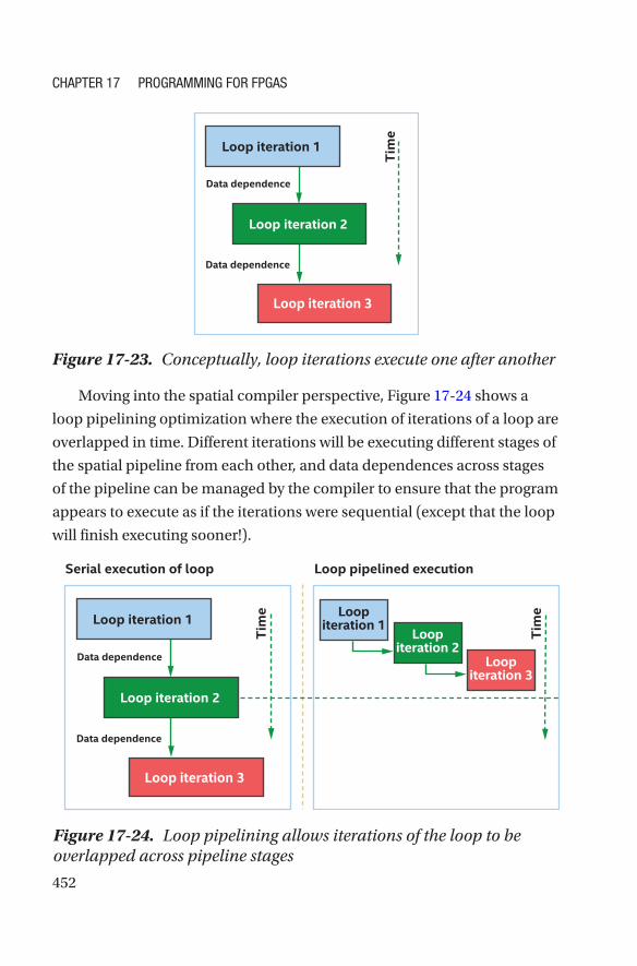
Conceptually, we probably think of iterations of a loop in C++ as executing

one after another, as shown in Figure 17-23. That’s the programming

model and is the right way to think about loops. In implementation,

though, compilers are free to perform many optimizations as long as most

behavior (i.e., defined and race-free behavior) of the program doesn’t

observably change. Regardless of compiler optimizations, what matters is

that the loop appears to execute as if Figure 17-23 is how it happened.


452

Figure 17-24. Loop pipelining allows iterations of the loop to be overlapped across pipeline stages

Figure 17-23. Conceptually, loop iterations execute one after another

Moving into the spatial compiler perspective, Figure 17-24 shows a

loop pipelining optimization where the execution of iterations of a loop are

overlapped in time. Different iterations will be executing different stages of

the spatial pipeline from each other, and data dependences across stages

of the pipeline can be managed by the compiler to ensure that the program

appears to execute as if the iterations were sequential (except that the loop

will finish executing sooner!).


453

Loop pipelining is easy to understand with the realization that many

results within a loop iteration may finish computation well before the loop

iteration finishes all of its work and that, in a spatial pipeline, results can

be passed to an earlier pipeline stage when the compiler decides to do so.

Figure 17-25 shows this idea where the results of stage 1 are fed backward

in the pipeline, allowing a future loop iteration to use the result early,

before the previous iteration has completed.

With loop pipelining, it is possible for the execution of many iterations

of a loop to overlap. The overlap means that even with loop-carried data

dependences, loop iterations can still be used to fill the pipeline with work,

leading to efficient utilization. Figure 17-26 shows how loop iterations

might overlap their executions, even with loop-carried data dependences,

within the same simple pipeline as was shown in Figure 17-25.

Figure 17-25. A pipelined implementation of the incremental random number generator


454

In real algorithms, it is often not possible to launch a new loop iteration

every single clock cycle, because a data dependence may take multiple

clock cycles to compute. This often arises if memory lookups, particularly

from off-chip memories, are on the critical path of the computation of

a dependence. The result is a pipeline that can only initiate a new loop

iteration every N clock cycles, and we refer to this as an initiation interval

(II) of N cycles. An example is shown in Figure 17-27. A loop initiation

interval (II) of two means that a new loop iteration can begin every second

cycle, which results in sub-optimal occupancy of the pipeline stages.

Figure 17-26. Loop pipelining simultaneously processes parts of multiple loop iterations


455

An II larger than one can lead to inefficiency in the pipeline because

the average occupancy of each stage is reduced. This is apparent from

Figure 17-27 where II=2 and pipeline stages are unused a large percentage

(50%!) of the time. There are multiple ways to improve this situation.

The compiler performs extensive optimization to reduce II whenever

possible, so its reports will also tell us what the initiation interval of each

loop is and give us information on why it is larger than one, if that occurs.

Restructuring the compute in a loop based on the reports can often reduce

the II, particularly because as developers, we can make loop structural

changes that the compiler isn’t allowed to (because they would be

observable). Read the compiler reports to learn how to reduce the II in

specific cases.

An alternative way to reduce inefficiency from an II that is larger than

one is through nested loops, which can fill all pipeline stages through

interleaving of outer loop iterations with those of an inner loop that has

II>1. Check vendor documentation and the compiler reports for details on

using this technique.

Figure 17-27. Sub-optimal occupancy of pipeline stages


456

PipesAn important concept in spatial and other architectures is a first-in first-

out (FIFO) buffer. There are many reasons that FIFOs are important, but

two properties are especially useful when thinking about programming:

1. There is implicit control information carried alongside the data. These signals tell us whether

the FIFO is empty or full and can be useful when

decomposing a problem into independent pieces.

2. FIFOs have storage capacity. This can make it

easier to achieve performance in the presence of

dynamic behaviors such as highly variable latencies

when accessing memory.

Figure 17-28 shows a simple example of a FIFO’s operation.

Figure 17-28. Example operation of a FIFO over time


457

FIFOs are exposed in DPC++ through a feature called pipes. The main

reason that we should care about pipes when writing FPGA programs is

that they allow us to decompose a problem into smaller pieces to focus on

development and optimizations in a more modular way. They also allow

the rich communication features of the FPGA to be harnessed. Figure 17- 29

shows both of these graphically.

Figure 17-29. Pipes simplify modular design and access to hardware peripherals

Remember that FPGA kernels can exist on the device simultaneously

(in different areas of the chip) and that in an efficient design, all parts

of the kernels are active all the time, every clock cycle. This means that

optimizing an FPGA application involves considering how kernels or parts

of kernels interact with one another, and pipes provide an abstraction to

make this easy.

Pipes are FIFOs that are implemented using on-chip memories on

an FPGA, so they allow us to communicate between and within running

kernels without the cost of moving data to off-chip memory. This provides

inexpensive communication, and the control information that is coupled

with a pipe (empty/full signals) provides a lightweight synchronization

mechanism.


458

DO WE NEED PIPES?

no. it is possible to write efficient kernels without using pipes. We can use all

of the FPGA resources and achieve maximum performance using conventional

programming styles without pipes. But it is easier for most developers to

program and optimize more modular spatial designs, and pipes are a great

way to achieve this.

As shown in Figure 17-30, there are four general types of pipes

available. In the rest of this section, we’ll cover the first type (inter-kernel

pipes), because they suffice to show what pipes are and how they are used.

Pipes can also communicate within a single kernel and with the host or

input/output peripherals. Please check vendor documentation for more

information on those forms and uses of pipes that we don’t have room to

dive into here.

Figure 17-30. Types of pipe connectivity in DPC++


459

A simple example is shown in Figure 17-31. In this case, there are

two kernels that communicate through a pipe, with each read or write

operating on a unit of an int.

// Create alias for pipe type so that consistent across usesusing my_pipe = pipe<class some_pipe, int>;

// ND-range kernelQ.submit([&](handler& h) {

auto A = accessor(B_in, h);

h.parallel_for(count, [=](auto idx) {my_pipe::write( A[idx] );

});});

// Single_task kernelQ.submit([&](handler& h) {

auto A = accessor(B_out, h);

h.single_task([=]() {for (int i=0; i < count; i++) {A[i] = my_pipe::read();

}});

});

Figure 17-31. Pipe between two kernels: (1) ND-range and (2) single task with a loop

There are a few points to observe from Figure 17-31. First, two kernels

are communicating with each other using a pipe. If there are no accessor

or event dependences between the kernels, the DPC++ runtime will

execute both at the same time, allowing them to communicate through the

pipe instead of full SYCL memory buffers or USM.

Pipes are identified using a type-based approach, where each is

identified using a parameterization of the pipe type which is shown in

Figure 17-32. The parameterization of the pipe type identifies a specific


460

pipe. Reads or writes on the same pipe type are to the same FIFO. There

are three template parameters that together define the type and therefore

identity of a pipe.

template <typename name,typename dataT,size_t min_capacity = 0>

class pipe;

Figure 17-32. Parameterization of the pipe type

It is recommended to use type aliases to define our pipe types, as

shown in the first line of code in Figure 17-31, to reduce programming

errors and improve code readability.

Use type aliases to identify pipes. this simplifies code and prevents accidental creation of unexpected pipes.

Pipes have a min_capacity parameter. It defaults to 0 which is

automatic selection, but if specified, it guarantees that at least that number

of words can be written to the pipe without any being read out. This

parameter is useful when

1. Two kernels communicating with a pipe do not run

at the same time, and we need enough capacity in

the pipe for a first kernel to write all of its outputs

before a second kernel starts to run and reads from

the pipe.

2. If kernels generate or consume data in bursts, then

adding capacity to a pipe can provide isolation

between the kernels, decoupling their performance

from each other. For example, a kernel producing


461

data can continue to write (until the pipe capacity

becomes full), even if a kernel consuming that data

is busy and not ready to consume anything yet. This

provides flexibility in execution of kernels relative

to each other, at the cost only of some memory

resources on the FPGA.

Blocking and Non-blocking Pipe Accesses

Like most FIFO interfaces, pipes have two styles of interface: blocking and

non-blocking. Blocking accesses wait (block/pause execution!) for the

operation to succeed, while non-blocking accesses return immediately

and set a Boolean value indicating whether the operation succeeded.

The definition of success is simple: If we are reading from a pipe and

there was data available to read (the pipe wasn’t empty), then the read

succeeds. If we are writing and the pipe wasn’t already full, then the write

succeeds. Figure 17-33 shows both forms of access member functions of

the pipe class. We see the member functions of a pipe that allow it to be

written to or read from. Recall that accesses to pipes can be blocking or

non-blocking.

// BlockingT read();void write( const T &data );

// Non-blockingT read( bool &success_code );void write( const T &data, bool &success_code );

Figure 17-33. Member functions of a pipe that allow it to be written to or read from


462

Both blocking and non-blocking accesses have their uses depending

on what our application is trying to achieve. If a kernel can’t do any more

work until it reads data from the pipe, then it probably makes sense to use

a blocking read. If instead a kernel wants to read data from any one of a

set of pipes and it is not sure which one might have data available, then

reading from pipes with a non-blocking call makes more sense. In that

case, the kernel can read from a pipe and process the data if there was any,

but if the pipe was empty, it can instead move on and try reading from the

next pipe that potentially has data available.

For More Information on Pipes

We could only scratch the surface of pipes in this chapter, but we should

now have an idea of what they are and the basics of how to use them. FPGA

vendor documentation has a lot more information and many examples of

their use in different types of applications, so we should look there if we

think that pipes are relevant for our particular needs.

Custom Memory SystemsWhen programming for most accelerators, much of the optimization effort

tends to be spent making memory accesses more efficient. The same

is true of FPGA designs, particularly when input and output data pass

through off-chip memory.

There are two main reasons that memory accesses on an FPGA can be

worth optimizing:

1. To reduce required bandwidth, particularly if some

of that bandwidth is used inefficiently

2. To modify access patterns on a memory that is

leading to unnecessary stalls in the spatial pipeline


463

It is worth talking briefly about stalls in the spatial pipeline. The

compiler builds in assumptions about how long it will take to read from

or write to specific types of memories, and it optimizes and balances the

pipeline accordingly, hiding memory latencies in the process. But if we

access memory in an inefficient way, we can introduce longer latencies

and as a by-product stalls in the pipeline, where earlier stages cannot make

progress executing because they’re blocked by a pipeline stage that is

waiting for something (e.g., a memory access). Figure 17-34 shows such a

situation, where the pipeline above the load is stalled and unable to make

forward progress.

Figure 17-34. How a memory stall can cause earlier pipeline stages to stall as well


464

There are a few fronts on which memory system optimizations can be

performed. As usual, the compiler reports are our primary guide to what

the compiler has implemented for us and what might be worth tweaking or

improving. We list a few optimization topics here to highlight some of the

degrees of freedom available to us. Optimization is typically available both

through explicit controls and by modifying code to allow the compiler to

infer the structures that we intend. The compiler static reports and vendor

documentation are key parts of memory system optimization, sometimes

combined with profiling tools during hardware executions to capture

actual memory behavior for validation or for the final stages of tuning.

1. Static coalescing: The compiler will combine

memory accesses into a smaller number of wider

accesses, where it can. This reduces the complexity

of a memory system in terms of numbers of load

or store units in the pipeline, ports on the memory

system, the size and complexity of arbitration

networks, and other memory system details.

In general, we want to enable static coalescing

wherever possible, which we can confirm through

the compiler reports. Simplifying addressing logic in

a kernel can sometimes be enough for the compiler

to perform more aggressive static coalescing, so

always check in the reports that the compiler has

inferred what we expect!

2. Memory access style: The compiler creates load

or store units for memory accesses, and these are

tailored to both the memory technology being

accessed (e.g., on-chip vs. DDR vs. HBM) and the

access pattern inferred from the source code (e.g.,

streaming, dynamically coalesced/widened, or


465

likely to benefit from a cache of a specific size).

The compiler reports tell us what the compiler has

inferred and allow us to modify or add controls to

our code, where relevant, to improve performance.

3. Memory system structure: Memory systems (both

on- and off-chip) can have banked structures

and numerous optimizations implemented by

the compiler. There are many controls and mode

modifications that can be used to control these

structures and to tune specific aspects of the spatial

implementation.

Some Closing TopicsWhen talking with developers who are getting started with FPGAs, we find

that it often helps to understand at a high level the components that make

up the device and also to mention clock frequency which seems to be a

point of confusion. We close this chapter with these topics.

FPGA Building BlocksTo help with an understanding of the tool flows (particularly compile

time), it is worth mentioning the building blocks that make up an

FPGA. These building blocks are abstracted away through DPC++

and SYCL, and knowledge of them plays no part in typical application

development (at least in the sense of making code functional). Their

existence does, however, factor into development of an intuition for spatial

architecture optimization and tool flows, and occasionally in advanced

optimizations when choosing the ideal data type for our application, for

example.


466

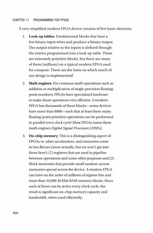
A very simplified modern FPGA device consists of five basic elements.

1. Look-up tables: Fundamental blocks that have a

few binary input wires and produce a binary output.

The output relative to the inputs is defined through

the entries programmed into a look-up table. These

are extremely primitive blocks, but there are many

of them (millions) on a typical modern FPGA used

for compute. These are the basis on which much of

our design is implemented!

2. Math engines: For common math operations such as

addition or multiplication of single-precision floating-

point numbers, FPGAs have specialized hardware

to make those operations very efficient. A modern

FPGA has thousands of these blocks—some devices

have more than 8000—such that at least these many

floating-point primitive operations can be performed

in parallel every clock cycle! Most FPGAs name these

math engines Digital Signal Processors (DSPs).

3. On-chip memory: This is a distinguishing aspect of

FPGAs vs. other accelerators, and memories come

in two flavors (more actually, but we won’t get into

those here): (1) registers that are used to pipeline

between operations and some other purposes and (2)

block memories that provide small random-access

memories spread across the device. A modern FPGA

can have on the order of millions of register bits and

more than 10,000 20 Kbit RAM memory blocks. Since

each of those can be active every clock cycle, the

result is significant on-chip memory capacity and

bandwidth, when used efficiently.


467

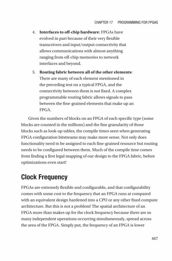
4. Interfaces to off-chip hardware: FPGAs have

evolved in part because of their very flexible

transceivers and input/output connectivity that

allows communications with almost anything

ranging from off-chip memories to network

interfaces and beyond.

5. Routing fabric between all of the other elements:

There are many of each element mentioned in

the preceding text on a typical FPGA, and the

connectivity between them is not fixed. A complex

programmable routing fabric allows signals to pass

between the fine-grained elements that make up an

FPGA.

Given the numbers of blocks on an FPGA of each specific type (some

blocks are counted in the millions) and the fine granularity of those

blocks such as look-up tables, the compile times seen when generating

FPGA configuration bitstreams may make more sense. Not only does

functionality need to be assigned to each fine-grained resource but routing

needs to be configured between them. Much of the compile time comes

from finding a first legal mapping of our design to the FPGA fabric, before

optimizations even start!

Clock FrequencyFPGAs are extremely flexible and configurable, and that configurability

comes with some cost to the frequency that an FPGA runs at compared

with an equivalent design hardened into a CPU or any other fixed compute

architecture. But this is not a problem! The spatial architecture of an

FPGA more than makes up for the clock frequency because there are so

many independent operations occurring simultaneously, spread across

the area of the FPGA. Simply put, the frequency of an FPGA is lower


468

than other architectures because of the configurable design, but more

happens per clock cycle which balances out the frequency. We should

compare compute throughput (e.g., in operations per second) and not raw

frequency when benchmarking and comparing accelerators.

This said, as we approach 100% utilization of the resources on an

FPGA, operating frequency may start to decrease. This is primarily a result

of signal routing resources on the device becoming overused. There are

ways to remedy this, typically at the cost of increased compile time. But

it’s best to avoid using more than 80–90% of the resources on an FPGA for

most applications unless we are willing to dive into details to counteract

frequency decrease.

Rule of thumb try not to exceed 90% of any resources on an FPGA and certainly not more than 90% of multiple resources. exceeding may lead to exhaustion of routing resources which leads to lower operating frequencies, unless we are willing to dive into lower-level FPGA details to counteract this.

SummaryIn this chapter, we have introduced how pipelining maps an algorithm to

the FPGA’s spatial architecture. We have also covered concepts that can

help us to decide whether an FPGA is useful for our applications and that

can help us get up and running developing code faster. From this starting

point, we should be in good shape to browse vendor programming and

optimization manuals and to start writing FPGA code! FPGAs provide

performance and enable applications that wouldn’t make sense on other

accelerators, so we should keep them near the front of our mental toolbox!


469

Open Access This chapter is licensed under the terms

of the Creative Commons Attribution 4.0 International

License (http://creativecommons.org/licenses/by/4.0/), which permits

use, sharing, adaptation, distribution and reproduction in any medium or

format, as long as you give appropriate credit to the original author(s) and

the source, provide a link to the Creative Commons license and indicate if

changes were made.

The images or other third party material in this chapter are included

in the chapter’s Creative Commons license, unless indicated otherwise

in a credit line to the material. If material is not included in the chapter’s

Creative Commons license and your intended use is not permitted by

statutory regulation or exceeds the permitted use, you will need to obtain

permission directly from the copyright holder.


http://creativecommons.org/licenses/by/4.0/

Documents

Programming for FPGAs