Program on the Global Demography of Aging · The Program on the Global Demography of Aging ... We develop a life-cycle model of optimal retirement and savings behavior under complete

HARVARD INITIATIVE FOR GLOBAL HEALTH

WORKING PAPER SERIES

Program on the Global Demography of Aging

THE EFFECT OF IMPROVEMENTS IN HEALTH AND LONGEVITY

ON OPTIMAL RETIREMENT AND SAVING David E. Bloom, David Canning, Michael Moore

Working Paper No. 2

April 2005 http://www.globalhealth.harvard.edu/WorkingPapers.aspx The views expressed in this paper are those of the author(s) and not necessarily those of the Harvard Initiative for Global Health. The Program on the Global Demography of Aging receives funding from the National Institute on Aging, Grant No. 1 P30 AG024409-01. ©2005 by David E. Bloom, David Canning, and Michael Moore. All rights reserved.

ABSTRACT

We develop a life-cycle model of optimal retirement and savings behavior under complete markets where retirement is caused by worsening health in old age. Our model explains the long-run decline in the age of retirement as an income level effect. We show that improvements in health and longevity tend to increase the desired retirement age, though less than proportionately, while, contrary to conventional views, reducing savings rates. The retirement age is not simply proportional to healthy lifespan because compound interest creates a wealth effect when lifespan increases, leading to more leisure (early retirement) and higher consumption (lower savings). David E. Bloom Harvard School of Public Health Department of Population and International Health 677 Huntington Ave. Boston, MA 02115 Email: [email protected] David Canning Harvard School of Public Health Department of Population and International Health 677 Huntington Ave. Boston, MA 02115 Email: [email protected] Michael Moore School of Management and Economics Queen’s University Belfast University Road Belfast BT7 1NN Email: [email protected]

1

mailto:[email protected]

HARVARD INITIATIVE FOR GLOBAL HEALTH WORKING PAPER NO. 2

I. INTRODUCTION

Among the most remarkable changes in human welfare that took place in the 20th century

was the improvement in health and the related rise in life expectancy. For the world as a

whole, life expectancy at birth rose from around 30 years in 1900 to 65 years by 2000 (and

is projected to rise to 81 by the end of this century; Lee, 2003). These improvements have

not only resulted in a large direct gain in welfare (Nordhaus, 2003), but have presumably

also had a profound influence on economic life-cycle behavior by changing people’s time

horizons (Hamermesh, 1985).

We focus on two fundamental, interrelated issues in life-cycle behavior, namely,

retirement and consumption patterns. One of the central reasons for saving is to provide

income for retirement. This life-cycle theory of saving and retirement is not a complete

model. For example, people also engage in precautionary savings to guard against income

shocks, and they may save to provide bequests. In addition, in many developing countries

the elderly are supported to a large extent by intra-family transfers, while many industrial

countries have widespread social security systems which support the elderly. These

transfer systems clearly affect incentives to save and to retire.

Notwithstanding its incompleteness, the life-cycle model can provide valuable

insights into behavior. In this paper we develop a theoretical model of retirement and

consumption based on individual optimization over the life-cycle with complete and

perfect capital markets. As well as offering a positive theory for observed behavior, such

an approach offers an insight into the welfare effects of proposed changes to social security

2


systems. Many social security systems are based on pay-as-you-go financing, which

involves transfers from current workers to current retirees. Increased life expectancies,

together with low birth rates, promote aging populations, which can impose great financial

stress on such systems. As a result, increases in contribution rates for workers, reductions

in benefits to retirees, or increases in the age of retirement may be necessary to ensure

financial solvency. Insofar as social security systems try to promote the optimal retirement

and consumption outcomes rational agents would make with perfect markets, in an effort

to overcome widespread lack of foresight about the need to save for retirement, time

inconsistency in preferences (Feldstein, 1985; Laibson, 1998; Laibson et al. 1998), or

capital market imperfections (Hubbard and Judd, 1987), the results of our model can serve

as benchmarks in the design of public pension systems. It is important to note, however,

that our model does not take into account possible negative externalities on others that

occur if people suffer an impoverished old age (Kotlikoff, Spivak, and Summers, 1982), or

potential welfare gains from intergenerational transfers as, for example, in Samuelson

(1958). These effects might make the optimal social security system have higher levels of

forced saving, or a redistributional element.

Several papers have tackled the issue of how changes in longevity affect retirement

and consumption decisions. The two most similar to our approach are Chang (1991) and

Kalemli-Ozcan and Weil (2002). In these papers agents maximize lifetime utility over

consumption and leisure, and the optimal retirement age and optimal consumption profile

over time are jointly determined. Both papers emphasize the possibility that while longer

lifetimes typically increase the optimal retirement age, under some circumstances the

3


desired age of retirement may decline as life expectancy increases. A key mechanism for

this to occur is an imperfect annuity market, so that in an environment with a high death

rate the return to saving is uncertain, because the wealth stock accumulated is likely to be

wasted when the agent dies. When life expectancy increases and mortality falls this

“uncertainty effect” declines, and the prospect of saving for retirement becomes more

appealing. In addition, these papers assume that increases in life expectancy have no effect

on health and the disutility of working at each age, so that any incentive to retire early

because of poor health remains unchanged.

We assume complete capital markets; in particular, the existence of (perfect)

annuity markets. However, the major innovation in this paper is to model health during the

agent’s lifetime and its effect on the decision to retire. Rather than impose a fixed

disutility of working, we assume that the disutility of work depends on a worker’s health

status. A great deal of evidence indicates that retirement is linked to poor health (see, for

example, Sickles and Taubman, 1986), although there are serious concerns about the

accuracy of health measurements (Bound, 1991).

An important feature of our model is our assumption that rising life expectancy

goes hand in hand with improved health status at each age (that is, we examine a lifespan

that is both longer and healthier). Increases in life expectancy in the United States over the

last two centuries have indeed been associated with reductions in the age-specific

incidence of disease, disability, and morbidity (Costa, 1998a; Fogel, 1994, 1997). Mathers

et al. (2001) show that health-adjusted life expectancy (each life year weighted by a

measure of health status) rises approximately one for one with life expectancy across

4


countries. This motivates us to use a model in which health status rises with life

expectancy, so that the age of onset of illnesses that increase the disutility of labor rises

proportionately with life expectancy.

In our analysis we find that the behavioral effect of improved health and longevity

on optimal retirement age is ambiguous, but we can determine the direction of the effect

under “reasonable” assumptions. For example, we assume that the optimal retirement age

is less than life expectancy, which seems plausible in industrial countries, but may be a less

appealing assumption in developing countries. In addition, we assume that interest rates

are not “too high” and are comparable to the rate of time preference.

Using this framework, we show that the effect of increases in health and life

expectancy is to increase the optimal retirement age, although it rises less than

proportionately with longevity, so that the fraction of the lifespan spent in retirement rises.

At the same time, consumption at each age rises and savings rates fall.

This result contrasts with the argument that an increase in longevity and an

increased need for retirement income may have been a driving force for increases in

savings, particularly the boom in household savings in East Asia over the last fifty years

(see Bloom, Canning, and Graham, 2003; Lee, Mason, and Miller, 2000; and Tsai, Chu,

and Chung, 2000). Deaton and Paxson (2000) point out that this savings effect seems

reasonable when the retirement age is fixed, but argue that in a flexible economy, without

mandatory retirement, the main effect of a rise in longevity will be on the span of the

working life, with no obvious prediction for the rate of saving. Kotlikoff (1989) similarly

argues that the main effect of a rise in longevity will be on the length of the working life

5


and analyses the effect on the economy when working life increases proportionately, and

when it rises an equal number of years (that is, more than proportionately). We formalize

the analysis of savings behavior in response to increased longevity when the retirement age

is endogenous and have the prediction of a less than proportional rise in the retirement age

and a decrease in the savings rate.

This new result arises primarily because we allow for an improvement in health

when life expectancy rises, which encourages a longer working life because of a lower

disutility of labor. At first sight, it is tempting to imagine a proportionality result where

working life is proportional to life expectancy, and consumption and the saving rate remain

unchanged. However, this conjecture ignores the fact that the agent’s longer working life

permits greater exploitation of the accumulation of compound interest on savings. The

increased opportunity to exploit the benefits of compound interest generates higher

potential wealth at retirement than before; this “wealth effect” of a longer lifespan allows

for both an increase in leisure, in the form of the proportion of the lifespan spent in

retirement, along with somewhat higher consumption (and hence lower saving) at each

age, assuming that both consumption and leisure are normal goods.

Our results lead us to argue that the long-term decline in the age of retirement in

industrial countries over the last 150 years (Costa, 1998b) has not been due to

improvements in health and life expectancy; instead, we point to the potentially large effect

of the level of wages as a driving force behind earlier retirement, which coincides with

Costa’s (1998a) analysis. Our model also suggests that the emergence of jobs with lower

disutility of labor, lower interest rates and higher wage growth lead to a delay in

6


retirement, and may help explain the recent rise in the average age at retirement in the

United States (though Friedberg and Webb, 2003 emphasize institutional changes as the

explanation).

In our model we treat the interest rate, disutility of labor, rate of time preference

and rate of wage growth, as exogenous and fixed in our analysis of the effect of a rise in

life expectancy. In a general equilibrium model, aging populations may generate large

stocks of capital as they save for retirement, and this can drive down the return to capital,

lowering the long-run interest rate. Our model predicts that this will lead to longer

working lives, and lower savings rates among workers. However, Miles (1999) and

Poterba (2004) suggest that the returns to capital decline very slowly with expansions in

the capital stock and population aging in developed countries will lead to only a small

decline in the rate of return. Cutler, Poterba, Sheiner, and Summers (1990) suggest that

population aging and lower rates of labor force growth may increase the rate of technical

progress, which may lead to a higher rate of wage growth, though again the size of the

potential effect seems modest.

We examine retirement and savings in the context of complete markets. Of course,

our results would change dramatically in the presence of institutions or market

imperfections that limit choice or change the incentives for retirement and saving behavior.

As already noted, a lack of complete financial markets, particularly annuity markets,

increases the incentive to save as mortality rates fall. More directly, mandatory retirement

in some occupations may prevent individuals from responding optimally to longer

lifespans and force higher savings rates. Even in the absence of mandatory retirement,

7


substantial evidence indicates that retirement in industrial countries, particularly in

Western Europe, clusters around specific ages that depend on retirement incentives

inherent in the national social security system (Gruber and Wise, 1998).

Our model suggests that social security systems that have a mandatory age of

retirement, or that impose disincentives to work past a normal retirement age, may impose

a welfare loss, and that this loss is likely to become larger as health and longevity improve,

and the optimal retirement age rises. On the other hand, rising levels of income may

encourage early retirement making such constraints on the length of working life less

binding.1

We present our model in section II and show how the dynamic programming

problem facing agents generates a set of equations (derived from the first-order conditions)

that determine the optimal retirement age and consumption profile. In section III we find

solutions for the optimal retirement age and consumption profile and investigate how these

change with changes in the parameters of the model. Finding the optimal retirement age

and consumption rule in the simple case where the interest rate, rate of time preference,

and rate of wage growth are all zero is fairly straightforward. However, for the more

general case a full solution is not available, and we use the implicit function theorem to

derive an approximate solution that holds for the case where the rates of interest, time

preference, and wage growth are reasonably small. Section IV summarizes and discusses

our main results and suggests avenues for further research.

1 It is not necessary to set a retirement age for social security. An alternative system is to fix contribution levels and allow a free choice of retirement age with actuarially fair social security benefits, as is done in the United States and is being implemented in Sweden. Our model suggests that this type of system will lead agents to endogenously choose a higher retirement age as their health improves and their life expectancy rises.

8


II. THE MODEL

We examine the optimizing problem of agents deciding their lifetime labor supply and

consumption and take the real wage rate,ω , and interest rate, r, to be exogenous. We

assume that the interest rate is fixed over time, but that real wages grow at the rateσ ,

reflecting long-run economic growth.

For simplicity, we assume an exogenous, constant death rate; a more realistic

mortality schedule would allow for rising death rates as people age. We ignore the

possibility of using consumption and health services to extend longevity (Ehrlich and

Chuma, 1990), or of a reverse link from labor supply to health status and life expectancy.

We also assume that working life starts at the very beginning of the life cycle, with no

period of schooling. A more complete model would also allow for the endogenous choice

of schooling, along the lines of Kalemli-Ozcan, Ryder, and Weil (2000). In addition, we

assume that agents do not make bequests, which rules out a potential mechanism through

which changes in life expectancy among current and future generations can affect labor

supply and savings behavior (Skinner, 1985).

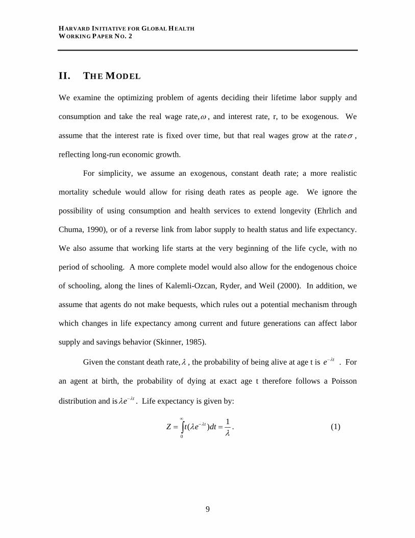
Given the constant death rate,λ , the probability of being alive at age t is te λ− . For

an agent at birth, the probability of dying at exact age t therefore follows a Poisson

distribution and is te λλ − . Life expectancy is given by:

0

1( )tZ t e dtλλλ

∞−= =∫ . (1)

9


Similarly we assume that health status is exogenously determined, evolving as a

function of life expectancy and age. Health may affect the productivity of workers and

their wage rate, as well as the desire for leisure, and may create a demand for the

consumption of health services. For simplicity, we assume that the only channel through

which health operates is the disutility of labor.

We assume that at age t the agent gets the instantaneous utility[ ]( ( )) ( , )tu c t v Z tχ− ,

where is felicity; is the disutility of working, assumed to be increasing in t;

and

( ( ))u c t ( , )v Z t

χ is an indicator function that takes the value 1 when working and 0 when retired. It

is not difficult to extend the model to allow for variable labor supply (i.e. partial

retirement), but in practice fixed costs associated with employment (for example,

commuting time) tend to make a discrete labor supply decision fairly common.

A major feature of our model is the disutility of labor schedule, , which rises

with age t and promotes retirement. In addition, we postulate that the disutility of working

at age t depends on life expectancy,

( , )v Z t

Z . If this disutility is independent of Z , it implies that

increases in life expectancy are not associated with general health improvements, and

population aging creates a large cohort of older people in poor health, which is at odds

with the evidence.

If health status at each age improves proportionately with life expectancy, then the

disutility of labor, , is homogeneous of degree zero in life expectancy and age as

follows:

( , )v Z t

( , ) ( ,v Z t v Z t)α α = (2)

10


In other words, the health status and disutility of working of someone working at age 45

who has a life expectancy of 60 is the same as the health status and disutility of someone

working at age 60 who has a life expectancy of 80.

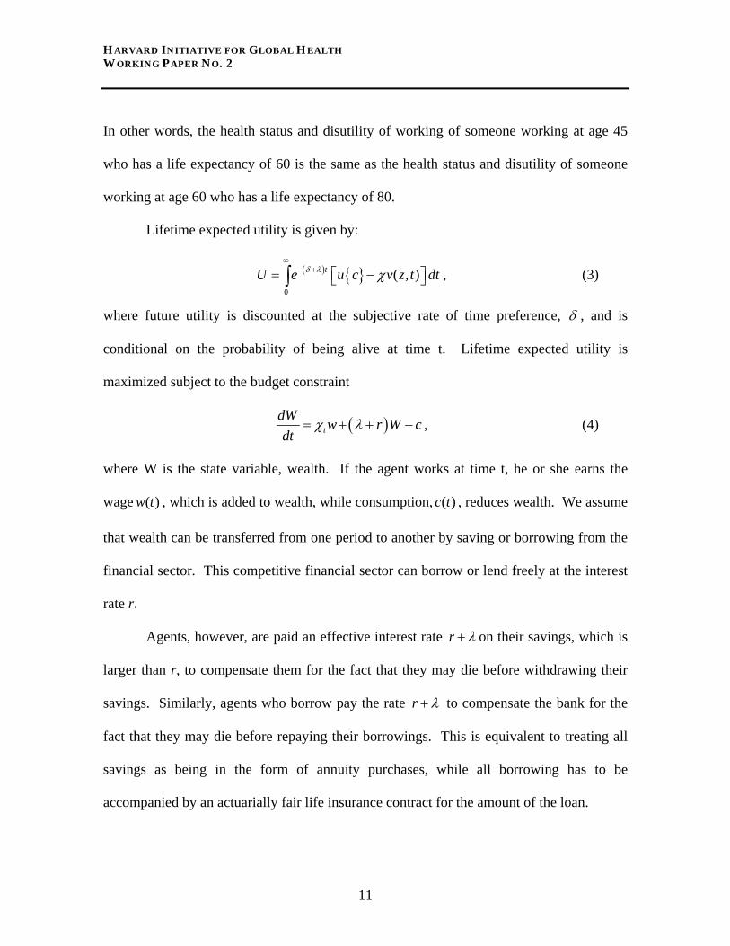
Lifetime expected utility is given by:

( ) { }0

( , )tU e u c v z t dδ λ χ∞

− += − t⎡ ⎤⎣ ⎦∫ , (3)

where future utility is discounted at the subjective rate of time preference, δ , and is

conditional on the probability of being alive at time t. Lifetime expected utility is

maximized subject to the budget constraint

( )tdW w r Wdt

χ λ c= + + − , (4)

where W is the state variable, wealth. If the agent works at time t, he or she earns the

wage , which is added to wealth, while consumption, , reduces wealth. We assume

that wealth can be transferred from one period to another by saving or borrowing from the

financial sector. This competitive financial sector can borrow or lend freely at the interest

rate r.

( )w t ( )c t

Agents, however, are paid an effective interest rate r λ+ on their savings, which is

larger than r, to compensate them for the fact that they may die before withdrawing their

savings. Similarly, agents who borrow pay the rate r λ+ to compensate the bank for the

fact that they may die before repaying their borrowings. This is equivalent to treating all

savings as being in the form of annuity purchases, while all borrowing has to be

accompanied by an actuarially fair life insurance contract for the amount of the loan.

11


Provided that a continuum of agents exists, the financial sector can avoid all risk by

aggregating over individuals and earns zero profits.

The transversality condition is that . Note that agents may plan to hold

positive wealth indefinitely, because they do not know how long they will live.

lim 0tt

W→∞

≥

2 The

control variables for the agent’s optimization problem are and c χ . Agents must decide

when to work and when to retire and what their consumption stream should be.

The Hamiltonian for this problem is:

( ) ( ){ } ( ) ( ) ( )( , ) ( )tt tH e u c t v z t w t r W t c tλ δ χ φ χ λ− + ⎡ ⎤= − + + + −⎡ ⎤⎣ ⎦⎣ ⎦ . (5)

The following are the first-order conditions for a maximum in and c χ :3

(H rW

)φ φ λ∂= − = − +

∂& , (6)

( ) ( ) 0tH e u cc

λ δ φ− +∂ ′= −∂

= , and (7)

( )

( )

( , ) ( ) 0 when 1

( , ) ( ) 0 when 0

t

t

H e v Z t w t

H e v Z t w t

λ δ

λ δ

φ χχ

φ χχ

− +

− +

∂= − + ≥ =

∂∂

= − + ≤ =∂

(8)

These conditions can be shown to yield the following:

( ) ( )( )

u cc r

u cδ

′= −

′′−& (9)

1 ( ) ( ) ( ,t u c w t v Z t)χ ′= ⇔ ≥ (10)

. 2 The transfer of the wealth of those who die to the financial sector exactly compensates deposit-taking institutions for the fact that they pay an interest rate r λ+ on deposits that exceed the risk free rate r, and rules out the need to consider unintended bequests. 3 Sydaeter, Storm, and Berck (1998) give sufficient conditions for a maximum. Checking that these conditions are satisfied for the explicit functional forms we employ later in the paper is straightforward.

12


The first condition implies a rising consumption level over time if the interest rate

is high, though this effect may be small if the utility function is highly concave. If the

marginal utility of consumption falls quickly with the level of consumption, that is,

is large, the agent will want to smooth consumption over time. The second

condition implies that agents work at time t so long as the utility gain from the

consumption purchased by the wage they earn (the marginal utility of consumption times

the wage) exceeds the disutility of working.

( )u c′′−

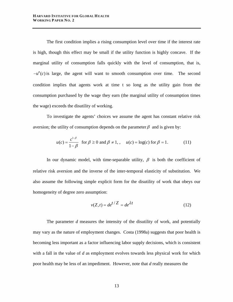
To investigate the agents’ choices we assume the agent has constant relative risk

aversion; the utility of consumption depends on the parameterβ and is given by:

1

( ) for 0 and 1, , ( ) log( ) for 11cu c u c c

β

β β ββ

−

= ≥ ≠ =−

= . (11)

In our dynamic model, with time-separable utility, β is both the coefficient of

relative risk aversion and the inverse of the inter-temporal elasticity of substitution. We

also assume the following simple explicit form for the disutility of work that obeys our

homogeneity of degree zero assumption:

/( , ) t Z tv Z t de deλ= = (12)

The parameter d measures the intensity of the disutility of work, and potentially

may vary as the nature of employment changes. Costa (1998a) suggests that poor health is

becoming less important as a factor influencing labor supply decisions, which is consistent

with a fall in the value of d as employment evolves towards less physical work for which

poor health may be less of an impediment. However, note that d really measures the

13


disutility of work relative to leisure, and the expansion in the range of leisure opportunities

available in old age may be increasing the attractiveness of retirement.

Our utility function implies that marginal utility is - ( )u c c β′ = and that the optimal

growth rate of consumption is:

(c rc

)δβ−

=&

, (13)

so that individual consumption is given by 0( )r t

c t c eδβ

⎛ ⎞−⎜ ⎟⎝ ⎠= . The initial level of

consumption, , can be calculated from a re-parameterization of the budget constraint as

follows:

0c

(14) ( ) ( )

0 0

( ) ( )R

r t r te c t dt e w tλ λ∞

− + − +=∫ ∫ dt

Using the result that the wage grows at the rateσ while consumption grows at the

rate r δβ− gives us:

( ) ( )0

0 0

r Rtr t r t te c e dt e w e

δλ λβ σ

⎛ ⎞−∞ ⎜ ⎟− + − +⎝ ⎠ =∫ ∫ 0 dt (15)

or

( )

( )

( 1)( )

0 0

0

0

( 1)

r t Rr tec wrr

β λβ δσ λβ

σ λβ λβ δβ

∞

⎛ ⎞− + +−⎜ ⎟ − +⎝ ⎠

⎡ ⎤⎢ ⎥ e⎡ ⎤⎢ ⎥ = ⎢ ⎥⎢ ⎥ − +⎛ ⎞− + + ⎣ ⎦−⎢ ⎥⎜ ⎟

⎝ ⎠⎣ ⎦

, (16)

and so

( )

( ) ( ( )0 0

( 1)1 r Rr

c w er

σ λβ λβ δβ λ σ

− −− + +=

+ −)− . (17)

14


For the model to make sense, we require that rσ λ< + . If this is not the case, the

net present value of lifetime wage earnings can be infinite and the budget constraint shown

in equation (15) is not well defined. Because we want to examine outcomes as the death

rate,λ , varies, we assume that rσ < so that the finite budget constraint holds for any death

rate.

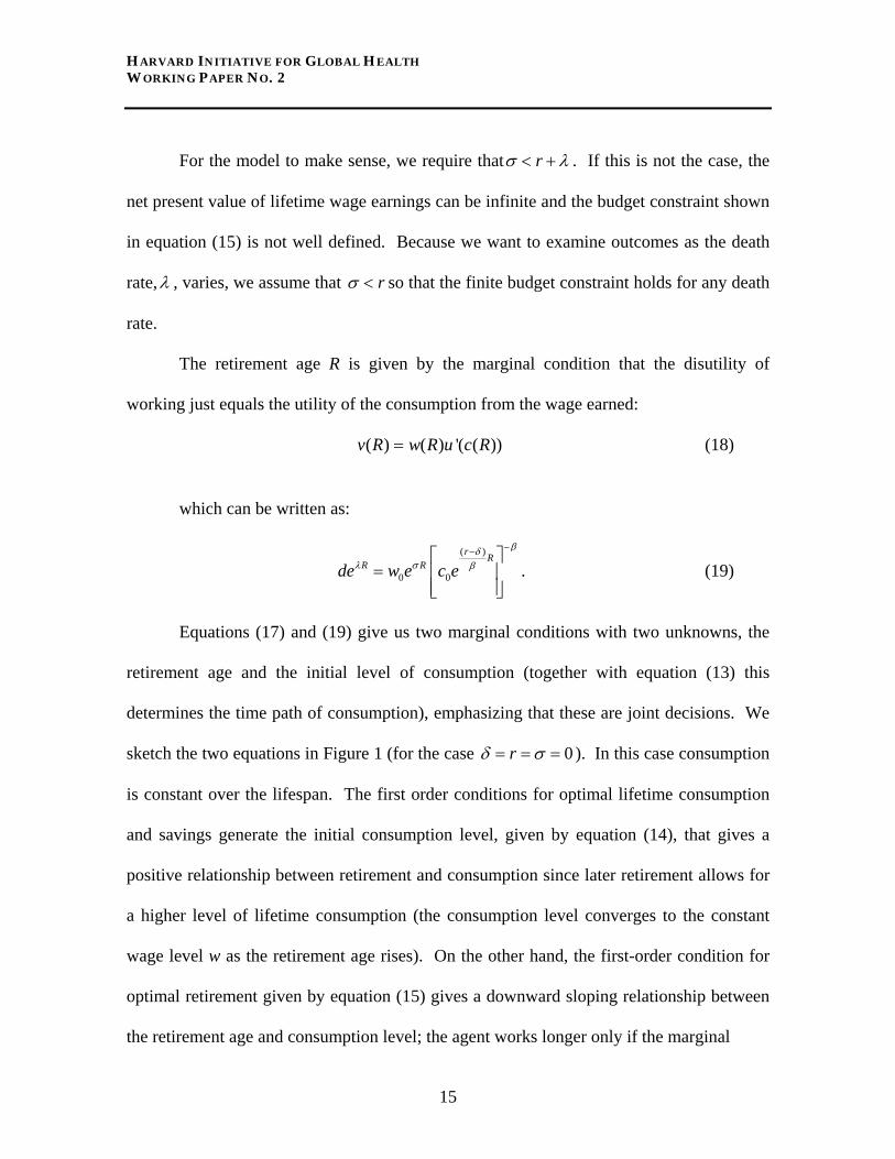
The retirement age R is given by the marginal condition that the disutility of

working just equals the utility of the consumption from the wage earned:

( ) ( ) '( ( ))v R w R u c R= (18)

which can be written as:

( )

0 0

r RR Rde w e c e

βδλ σ β

−−⎡ ⎤= ⎢ ⎥

⎢ ⎥⎣ ⎦. (19)

Equations (17) and (19) give us two marginal conditions with two unknowns, the

retirement age and the initial level of consumption (together with equation (13) this

determines the time path of consumption), emphasizing that these are joint decisions. We

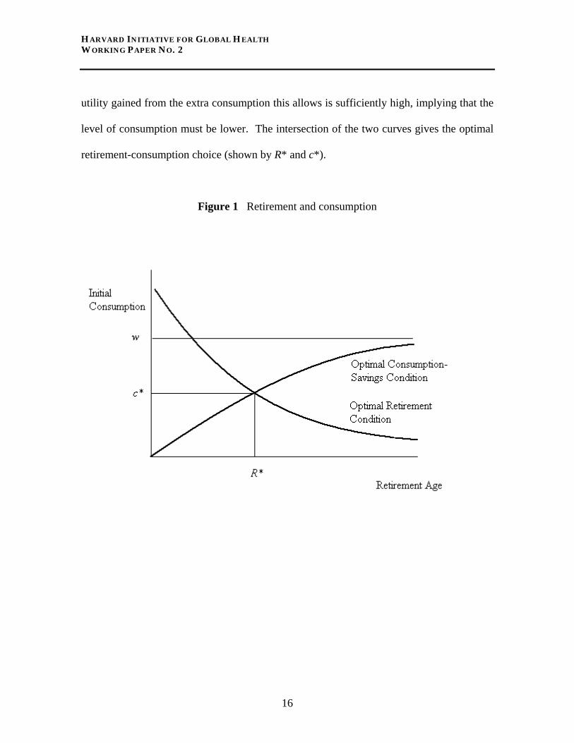
sketch the two equations in Figure 1 (for the case 0rδ σ= = = ). In this case consumption

is constant over the lifespan. The first order conditions for optimal lifetime consumption

and savings generate the initial consumption level, given by equation (14), that gives a

positive relationship between retirement and consumption since later retirement allows for

a higher level of lifetime consumption (the consumption level converges to the constant

wage level w as the retirement age rises). On the other hand, the first-order condition for

optimal retirement given by equation (15) gives a downward sloping relationship between

the retirement age and consumption level; the agent works longer only if the marginal

15


utility gained from the extra consumption this allows is sufficiently high, implying that the

level of consumption must be lower. The intersection of the two curves gives the optimal

retirement-consumption choice (shown by R* and c*).

Figure 1 Retirement and consumption

16


Substituting for the initial level of consumption in equation (19) gives:

( )( )0

( )1

( )( 1) (1 )

r RR

r R

r ede wr e

βσ δ

λ βσ λ

β λ σβ λβ δ

+ −−

− −

⎡ ⎤+ −= ⎢ ⎥− + + −⎣ ⎦

β , (20)

which is an implicit function of the retirement age R alone.4 Similarly, we substitute out

the retirement age in equation (19) and derive an equation that is an implicit function of ,

the initial level of consumption, alone:

0c

( )( )

0 00 0

( 1)1 ( )

rr

r w cc wr d

σ λβλ δ σ

β λβ δβ λ σ

− −−− − +

⎛ ⎞− + += −⎜+ − ⎝ ⎠

⎟ , (21)

We now have a set of equations that could provide the solution to the agent’s maximization

problem. Equation (20) can be solved to give the retirement age, R. Equation (21) can be

solved to give the initial level of consumption, , which together with equation (13) gives

us a complete solution for the agent’s labor supply and consumption decisions.

0c

III. RETIREMENT AND CONSUMPTION DECISIONS

We now apply our theoretical model to analyze the determinants of retirement and savings

behavior. In general, we cannot find explicit solutions to equations (20) and (21) for an

arbitrary value of β ; we therefore examine behavior for a particular value of β , the

coefficient of relative risk aversion. Evidence from the asset pricing literature implies that

a high value of β is required to explain the equity premium and the volatility of asset

prices. Chetty and Szeidl (2004) suggest that this requirement imposes a lower bound

4 If the rate of wage growth is extremely high while the disutility of labor grows slowly, this equation may have no finite solution. However, provided that rσ λ δ< + − , the growth rate of the disutility of labor dominates and the agent will eventually retire.

17


on β of at least 2. However, the low empirical estimates we have of the elasticity of labor

supply with respect to wages imply a low value forβ . Chetty (2003) argues that a value

of β as high as 2 can only be supported by the most extreme empirically estimated value

of the elasticity of labor supply to wage changes.5 We use a value of 2β = as our

benchmark for the utility function. (We also give results for the case where 1β = [log

utility] for comparison.)

While we have a potential solution, solving the implicit functions (20) and (21) for

R and is complex, and we cannot find a complete closed-form solution. Our approach

is to use the implicit function theorem to obtain an approximation around a special case for

which we do have a complete closed-form solution. This special case is where the rate of

time preference, rate of interest, and growth rate of wages are all zero (

0c

0rδ σ= = = ). For

this set of parameter values we can write equation (20) as:

0

1 (1 )R RZde w e Z

β

β

−−− ⎡ ⎤

= −⎢ ⎥⎣ ⎦

(22)

Clearly this is an implicit function of R Z and has a solution of the form given by:

0( , , )R f w dZ

β= . (23)

5 Chetty’s work indicates that most estimates of the elasticity imply a value of β close to unity.

18


In this case, the optimal retirement age is a fixed proportion of life expectancy, with the

proportion depending on the parameters of the agent’s utility function and on the wage

rate.

As 0r δ= = , consumption is clearly steady over time. The level of consumption is

fixed at the initial level, which is the solution to:

0 00 0

(1 ).dc ww c β−= − (24)

This implies that the optimal consumption level, which solves this equation, is independent

of life expectancy and can be written as:

0 0( , , )c g w d β= (25)

.

For 2β = and 0rδ σ= = = , we can solve these equations to give the complete

closed-form solution6 as follows:

0 00

0

1 2 1 4 1 4 1log ,

2 2dw dw dw

R Z cdw d

⎡ ⎤+ + + + −= ⎢ ⎥

⎢ ⎥⎣ ⎦

0=

. (26)

In terms of Figure 1, an increase in life expectancy shifts both curves to the right.

In order to maintain a given level of consumption with a longer lifespan, the agent must

work for a longer period, moving the curve representing first order condition for optimal

consumption-savings to the right. At the same time, at a given level of consumption, and

6 This is the unique solution; a second formal solution exists but it implies a negative retirement age.

19


marginal utility of earnings, an increase in health and lifespan reduces the disutility of

work and encourages a longer working life, moving the curve representing the first order

condition for optimal retirement to the right. When 0rδ σ= = = the net effect of the shift

in the two curves is to raise the retirement age proportionately with life expectancy,

without changing the level of consumption.

However, we want to get some idea of how changes in the interest rate and the rate

of growth of wages affect retirement and savings behavior. We also want to study how

changes in health and life expectancy affect retirement and consumption when rates of

time preference, interest, and wage growth are not zero.

We therefore proceed to find an approximation to the solution to equations (20) and

(21) by using the implicit function theorem to linearize the solution for R and around

the point

0c

0rδ σ= = = . This will give us a good approximation to the solution provided

that , ,r δ and σ are small. Appendix 1 shows how we go about carrying out this

approximation.7 When 2β = and , ,r δ and σ are small8, we have the approximation:

7 The details of the calculations for each slope in the approximation equations (27) and (28) are available in the web appendix at http://www.qub-efrg.com/uploads/Web_Appendix.ZIP. This file contains Mathematica notebooks for each calculation. 8 The results for 1β = (log utility) are given in Appendix 2.

20


0 0

0

0 0 2

0 0

0 0 2

00

0 0

0 2

0

1 2 1 4log

2

1 2 1 4 2log2 1 4

1 2 1 41 log(2) log1 4

1 2 1 4log 1

2

1 4

dw dwR Z

dw

dw dwZ

dw dw

dw dwZ r

dwdw

dw dwdw

Zdw

σ

δ

⎡ ⎤+ + += ⎢ ⎥

⎢ ⎥⎣ ⎦⎛ ⎞⎛ ⎞+ + +⎜ ⎟+ −⎜ ⎟⎜ ⎟⎜ ⎟+⎝ ⎠⎝ ⎠⎛ ⎞⎛ + + +⎜ ⎟+ + − ⎜ ⎟⎜ ⎟⎜ ⎟+ ⎝ ⎠⎝ ⎠⎛ ⎞⎛ ⎞+ + +⎜ ⎟−⎜ ⎟⎜ ⎟⎜ ⎟⎝ ⎠⎝ ⎠+

+

⎞ (27)

and for initial consumption we have:

0 00

0

2 00 0 2

0

0

1 4 1 1 4 1(2 )

2 4 1 4

41 4 1 ( 1 4 1) log( 1 4 1)

4 1 4

dw dwc Z r

d d dw

dwdw dwdw

Zd dw

σ

δ

+ − + −= + −

+

⎛+ − + + − ⎜ ⎟⎜ ⎟+ −⎝ ⎠+

+

⎞ (28)

Table 1 shows the effects on the retirement age and initial consumption of changes

in the parameters implied by these equations.

21


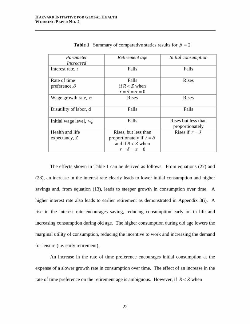
Table 1 Summary of comparative statics results for 2β =

Parameter Increased

Retirement age

Initial consumption

Interest rate, r

Falls Falls

Rate of time preference,δ

Falls if R Z< when

0r δ σ= = =

Rises

Wage growth rate, σ Rises

Rises

Disutility of labor, d

Falls Falls

Initial wage level, 0w Falls Rises but less than proportionately

Health and life expectancy, Z

Rises, but less than proportionately if r δ=

and if R Z< when 0r δ σ= = =

Rises if r δ=

The effects shown in Table 1 can be derived as follows. From equations (27) and

(28), an increase in the interest rate clearly leads to lower initial consumption and higher

savings and, from equation (13), leads to steeper growth in consumption over time. A

higher interest rate also leads to earlier retirement as demonstrated in Appendix 3(i). A

rise in the interest rate encourages saving, reducing consumption early on in life and

increasing consumption during old age. The higher consumption during old age lowers the

marginal utility of consumption, reducing the incentive to work and increasing the demand

for leisure (i.e. early retirement).

An increase in the rate of time preference encourages initial consumption at the

expense of a slower growth rate in consumption over time. The effect of an increase in the

rate of time preference on the retirement age is ambiguous. However, if R Z< when

22


0r δ σ= = = , then 0

0

1 2 1 4log

2dw dw

dw

⎡ ⎤+ + +⎢⎢ ⎥⎣ ⎦

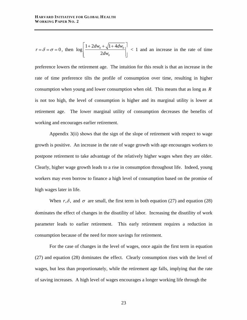
0 ⎥ < 1 and an increase in the rate of time

preference lowers the retirement age. The intuition for this result is that an increase in the

rate of time preference tilts the profile of consumption over time, resulting in higher

consumption when young and lower consumption when old. This means that as long as R

is not too high, the level of consumption is higher and its marginal utility is lower at

retirement age. The lower marginal utility of consumption decreases the benefits of

working and encourages earlier retirement.

Appendix 3(ii) shows that the sign of the slope of retirement with respect to wage

growth is positive. An increase in the rate of wage growth with age encourages workers to

postpone retirement to take advantage of the relatively higher wages when they are older.

Clearly, higher wage growth leads to a rise in consumption throughout life. Indeed, young

workers may even borrow to finance a high level of consumption based on the promise of

high wages later in life.

When , ,r δ and σ are small, the first term in both equation (27) and equation (28)

dominates the effect of changes in the disutility of labor. Increasing the disutility of work

parameter leads to earlier retirement. This early retirement requires a reduction in

consumption because of the need for more savings for retirement.

For the case of changes in the level of wages, once again the first term in equation

(27) and equation (28) dominates the effect. Clearly consumption rises with the level of

wages, but less than proportionately, while the retirement age falls, implying that the rate

of saving increases. A high level of wages encourages a longer working life through the

23


substitution effect. At the same time it makes workers richer, and the income effect leads

to a greater demand for leisure. For values of 1β > , the income effect dominates, leading

to earlier retirement. Indeed, rising income levels can potentially account for the long,

secular decline in the retirement age over the last 150 years in industrial countries.

An increase in health and life expectancy acts as an increase in endowment. When

, ,r δ and σ are all zero, an increase in health and life expectancy lead to a proportional

increase in working life, leaving the level of consumption during each period unchanged.

This is a general result, independent of the felicity function (as shown in Bloom, Canning,

and Graham 2003). The intuition for this is that an increase in health and life expectancy

can be thought of as stretching time, and can be formally captured by a simple change in

the time variable that leaves the optimization problem, expressed as a function of the

proportion of lifespan worked, unchanged.

When , ,r δ and σ are small, the first term in equation (27) dominates the effect of

an increase in life expectancy on retirement, so retirement still rises with life expectancy.

However, the proportion of life spent working declines, as shown in Appendix 3(iii). From

equation (28) it is clear that initial consumption rises in response to longer life expectancy

if r δ= ,9 and equation (13) implies that consumption rises throughout the life cycle.

Table 1 shows only the effect of life expectancy on retirement and consumption.

Now consider the effect on the savings rate during working life when life expectancy

increases. Higher consumption at each point in time, together with a lower total return on

9 This is a sufficient condition. The proof can clearly be relaxed to r kδ< for some k > 1.

24


savings due to a smallerλ and lower annuity rates, means that wealth rises more slowly

when life expectancy increases. Hence consumption rises, and income (including the

return on wealth) falls, reducing the observed saving rate of a worker at each age. This

reduced savings rate only holds when the comparison is between two workers. Eventually

the worker with the shorter lifespan will retire and have a low savings rate (out of a much

lower income), while the worker with a longer lifespan stays in employment and keeps

saving for retirement. However, conditional on being employed, a longer lifespan will

generate a lower savings rate at each age.

The intuition for this result is that an increase in life expectancy magnifies the

compounding effects of wage growth, interest rates, and time preference. For example,

suppose that only the interest rate is positive and the agent keeps to the proportionality

result that holds in the case of , ,r δ and σ all being zero when life expectancy rises. Now

when life expectancy rises, upon reaching retirement age the agent will have greater wealth

than before because of the increased effects of interest compounding over a longer working

life. The higher level of accumulated assets allows a higher level of consumption (spread

over the entire lifespan), which induces a lower marginal utility of consumption, reducing

the incentive to work and encouraging earlier retirement. The wealth effect generated by

compound interest over a longer lifespan leads to both an increase in consumption and an

increase in leisure (early retirement).

While the proportion of lifetime spent in employment falls as health and longevity

rise, it is important to note that absolute length of the working lifetime must increase

sufficiently to generate higher wealth at retirement than before despite a lower savings rate,

25


in order to finance a higher level of consumption over a longer period of retirement. This

indicates that the fall in the proportion of lifetime worked cannot be too great and that the

main effect of increased health and longevity is to increase the length of the working life.

IV. CONCLUSION

Our model demonstrates three major, long-term influences on the optimal age at retirement

and on savings behavior. First, at higher levels of lifetime income, the desire for increased

leisure leads to early retirement funded through a higher savings rate. Second, a lower

intrinsic disutility of working, as employment moves away from manual labor, leads to

longer working lives and less need to save for retirement, though this effect may be offset

by increased opportunities for leisure activities. Third, longer lifespans and healthier lives

lead to an increase in working life. However, the longer lifespan allows the enjoyment of

compound interest on savings for a longer period, and this leads to a reduction in both the

proportion (though not the number of years) of the lifespan spent in employment and in the

savings rate.

We also find effects due to the rate of time preference, the interest rate, and the rate

of wage growth. These variables may change, for example, the interest rate may fall with

increased levels of investment as aging populations save for retirement, and the rate of

wage growth may rise if the rate of technical progress increases. Changes in these

variables are, however, likely to be small.

While our model may help predict actual behavior, a more realistic approach would

allow for market imperfections, institutionalized transfer arrangements, and less than fully

26


rational behavior. However, our results do give the optimal retirement and savings

behavior of fully rational agents under complete and perfect capital markets, and can

therefore be thought of as a benchmark for the design of social security systems whose

objective is to promote such an outcome.

APPENDIX 1. LINEAR APPROXIMATION

Let 0( , , , , , )x w d rλ σ δ= . For 0 0( , , ,0,0,0)x w dλ= the retirement age is the implicit

solution to equation (20). Now define:

( )

( )0

( )1

( )( , )( 1) (1 )

r RR

r R

r eF R x de wr e

βσ δ

λ βσ λ

β λ σβ λβ δ

+ −−

− −

⎡ ⎤+ −= − ⎢ ⎥− + + −⎣ ⎦

β (29)

.

By the implicit function theorem we can write the optimal retirement age in the

neighborhood of x0 as a unique differentiable function:

0* ( ) * ( , , , , , )R x R w d rλ σ δ= (30)

where

( * ( ), ) 0F R x x = (31)

as long as the partial derivatives of F are continuous (which is clear) and ( , ) 0F R xR

∂≠

∂.

Furthermore the implicit function theorem implies that:

*

*

FdR xFdx

R

δδ

δδ

= − (32)

27


We can calculate this by differentiating F. Applying Taylor’s Theorem,

0

0 0** ( ) * ( ) ( )

x x

RR x R x x xx

δδ =

≈ + − (33)

.

We can expand this around 0 0( , , ,0,0,0)x w dλ= to give:

0 0

0* ** ( ) ( )

x x x x x x

R R RR x R x rr

σσ δ

0

*δ= = =

∂ ∂ ∂≈ + + +

∂ ∂ ∂ (34)

.

Similarly, we can use the implicit function:

( )

( )0 0

0 0 0

( 1)( , ) 1 ( )

rr

r w cG c x c w

r d

σ λβλ δ σ

β λβ δβ λ σ

− −−+ − −

⎛ ⎞− + += − −⎜

+ − ⎝ ⎠⎟ (35)

to derive an approximation for the initial level of consumption.

APPENDIX 2. THE CASE OF 1β =

Taking 1β = , which implies that felicity is logarithmic in consumption, and

assuming 0rδ σ= = = , our solution takes the simple form:

01log ,

1d

01R Z c w

d d+⎛ ⎞= =⎜ ⎟ +⎝ ⎠

. (36)

In this case, the wage level, , has no effect on the retirement age, R. In general, a higher

wage increases the incentive to work longer (the substitution effect), but it also raises

lifetime income and increases the demand for leisure and retirement (the income effect).

With log utility these income and substitution effects exactly cancel.

0w

28


Our first-order approximation to the optimal retirement age, which holds when

, ,r δ and σ are small, is:

( ) 2 2

1 1(1 ) log( ) 1 1 log( )1log(1 ) (1 )

d ddd d dR Z r Zd d d

Zσ δ

+ +⎡ ⎤ ⎡+ − −⎢ ⎥ ⎢+⎛ ⎞= + − −⎢ ⎥ ⎢⎜ ⎟ + +⎝ ⎠ ⎢ ⎥ ⎢⎣ ⎦ ⎣

⎤⎥⎥⎥⎦

. (37)

Similarly, we can find an approximation for initial consumption as follows:

00 02

11 log( )1 ( )1 (1 ) (1 )

ddw dc r Zwd d d

σ 02 Zwδ

++

= + − ++ + +

(38)

The details of the calculations for each slope in the approximation are available in

the web appendix at http://www.qub-efrg.com/uploads/Web_Appendix.ZIP.

Table 2 shows effects on behavior of changes in our parameters for 1β = .

29


Table 2 Summary of comparative statics results for 1β =

Parameter increased

Retirement age

Initial consumption

Interest rate, r

Falls Falls

Rate of time preference,δ

Falls if R Z< when

0r δ σ= = =

Rises

Wage growth rate, σ Rises

Rises

Disutility of labor, d Falls

Falls

Initial wage level, 0w Unchanged

Rises proportionately

Health and life expectancy, Z

Rises, but less than proportionately if R Z< when

0r δ σ= = =

Rises if r δ=

The results in Table 2 are very similar to those presented in Table 1. The main

difference is that the initial wage level now has no effect on the retirement age, with

consumption rising proportionately with the level of income (as opposed to less than

proportionately for the case of 2β = ). Most of the signs in Table 2 can be derived from

inspection of equations (37) and (38). Note that the condition R Z< when 0r δ σ= = =

now implies that 1log 1dd+⎛ ⎞ <⎜ ⎟

⎝ ⎠.

To ascertain the effect of both the interest rate and wage growth rate on the age at

retirement, note that 1(1 ) log( )ddd+

+ >1. To prove this, consider the following. For d =

0, the LHS is clearly infinite. Taylor’s theorem implies that log(1+x) is approximately

equal to x when x is small, so for d large we have that 1 1log(1 )d d

+ ≈ and the LHS 11d

≈ + .

30


Taking the limit as , this approximation becomes increasingly good and the

LHS .

d →∞

1→

We now argue that the slope of the LHS is never positive; this rules out LHS < 1

since that would imply a positive slope as the LHS rises to 1 as d gets large. Suppose that

LHS < 1 for some finite positive d0, then by the mean value theorem, a value d1 (between

d0 and ) exists for which the derivative of the LHS is positive. This implies that for d∞ 1,

1

1 1

1 1logd

d d+

> . Setting1

1cd

= , this implies that log(1 )c c+ > . Now consider the function

log(1 )x+ . For x = 0 we have log(1+0) = 0. Using the mean value theorem once again we

can find a k between 0 and c such that log(1 ) 1x k

d xdx =

+> , but this implies that 1 1

1 k>

+,

for k > 0, which is a contradiction.

The lack of any effect of the level of income on retirement in this case makes it

difficult to explain the long downward trend in the retirement age we have observed over

the last 150 years, and suggests that a value of β greater than one may be more realistic.

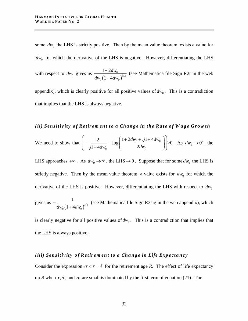
APPENDIX 3. SIGNING THE ELEMENTS OF TABLE 1

(i) Sensitivity of Retirement to a Change in the Interest Rate

We need to show that 0 0

00

1 2 1 41 log(2) log1 4

dw dwdwdw

⎛ ⎞⎛ ⎞+ + +⎜ ⎟+ − ⎜ ⎟⎜ ⎟⎜ ⎟+ ⎝ ⎠⎝ ⎠

<0.

As , the LHS approaches 0 0dw +→ −∞ . As , the LHS . Suppose that for 0dw →∞ 0→

31


some the LHS is strictly positive. Then by the mean value theorem, exists a value for

for which the derivative of the LHS is negative. However, differentiating the LHS

with respect to gives us

0dw

0dw

0dw( )

03 2

0 0

1 21 4

dwdw dw

+

+ (see Mathematica file Sign R2r in the web

appendix), which is clearly positive for all positive values of . This is a contradiction

that implies that the LHS is always negative.

0dw

(ii) Sensitivity of Retirement to a Change in the Rate of Wage Growth

We need to show that 0

00

1 2 1 42 log21 4

dw dwdwdw

⎛ ⎞⎛ ⎞+ + +⎜ ⎟− + ⎜ 0

⎜+ ⎝ ⎠⎝ ⎠0 0dw⎟⎟⎜ ⎟

>0. As +→ , the

LHS approaches . As , the LHS . Suppose that for some the LHS is

strictly negative. Then by the mean value theorem, a value exists for for which the

derivative of the LHS is positive. However, differentiating the LHS with respect to

gives us

+∞ 0dw →∞ 0→ 0dw

0dw

0dw

( )3 20 0

11 4dw dw

−+

(see Mathematica file Sign R2sig in the web appendix), which

is clearly negative for all positive values of . This is a contradiction that implies that

the LHS is always positive.

0dw

(iii) Sensitivity of Retirement to a Change in Life Expectancy

Consider the expression rσ δ< = for the retirement age R. The effect of life expectancy

on R when , ,r δ and σ are small is dominated by the first term of equation (21). The

32


coefficient on Z in this term is positive, which implies that retirement age increases with

life expectancy. To find the effect of increases in life expectancy on RZ

, we simply divide

through the expression for R by Z. The effect of Z on this ratio is now given by:

0 0

0 0

0 0

00

0 0

0

0

1 2 1 4 2log2 1 4

1 2 1 41 log(2) log1 4

1 2 1 4log 1

2

1 4

Rdw dwZ

Z dw dw

dw dwr

dwdw

dw dwdw

dw

σ

δ

∂ ⎛ ⎞⎛ ⎞+ + +⎜ ⎟= −⎜ ⎟⎜ ⎟⎜ ⎟∂ +⎝ ⎠⎝ ⎠

⎛ ⎞⎛ ⎞+ + +⎜ ⎟+ + − ⎜⎜⎜ ⎟+ ⎝ ⎠⎝ ⎠⎛ ⎞⎛ ⎞+ + +⎜ ⎟−⎜ ⎟⎜ ⎟⎜ ⎟⎝ ⎠⎝ ⎠+

+

⎟⎟ (39)

From our foregoing proofs, the coefficients on r and δ are both negative, as long as

R Z< when 0r δ σ= = = ; however, the coefficient on σ is positive. A sufficient

condition for

RZZ

∂

∂<0 is rσ δ≤ = (in addition to R Z< when 0r δ σ= = = ). In this case,

the derivative is bounded above by:

33


0 0

0 0

0 0

00

0 0

0

0

1 2 1 4 2log2 1 4

1 2 1 41 log(2) log1 4

1 2 1 4log 1

2

1 4

dw dwdw dw

dw dwr

dwdw

dw dwdw

dw

⎛ ⎞⎜ ⎟

⎛ ⎞⎜ + + +−⎜ ⎟⎜ ⎟⎜ ⎟ +⎜ ⎟⎝ ⎠

⎜ ⎟⎛ ⎞+ + +⎜ ⎟+ + − ⎜⎜ ⎟⎜+ ⎝ ⎠⎜ ⎟

⎜ ⎟⎛ ⎞+ + +⎜ ⎟−⎜ ⎟⎜ ⎟⎜ ⎟⎝ ⎠⎜ ⎟+

⎜ ⎟+⎝ ⎠

⎟

⎟⎟ (40)

which equals:

0 0

0

0

1 2 1 4log 2

2

1 4

dw dwdw

rdw

⎛ ⎞⎛ ⎞+ + +⎜ ⎟−⎜ ⎟⎜ ⎟⎜ ⎟⎝⎜

+⎜ ⎟⎜ ⎟⎜ ⎟⎝ ⎠

⎠⎟ (41)

This is clearly negative under our assumption that the retirement age is less than life

expectancy in the benchmark case.

34


V. REFERENCES

Bloom DE, Canning D, Graham B (2003). Longevity and life-cycle savings. Scandinavian Journal of Economics, 105:319–338. Bound J (1991). Self-reported versus objective measures of health in retirement models. Journal of Human Resources, 26:106–138. Chang FR (1991). Uncertain lifetimes, retirement, and economic welfare. Economica, 58: 215–232. Chetty R (2003). A new method of estimating risk aversion. NBER Working Paper No. 9988. Cambridge, National Bureau of Economic Research. Chetty R, Szeidl A (2004). Consumption commitments and asset prices. Working Paper. Berkeley, University of California, Economics Department. Costa DL (1998a). The evolution of retirement: an American economic history, 1880–1990. National Bureau of Economic Research Series on Long-Term Factors in Economic Development. Chicago, University of Chicago Press. Costa, Dora L (1998). The evolution of retirement: summary of a research project. American Economic Review, 88(2):232-236. Cutler DM, Poterba JM, Sheiner LM, Summers LH (1990). An aging society: opportunity or challenge? Brookings Papers on Economic Activity, 1:1-56. Deaton A, Paxson C (2000). Growth, demographic structure, and national saving in Taiwan. Population and Development Review, 26(Supplement):141-173. Ehrlich I, Chuma H (1990). A model of the demand for longevity and the value of life extension. Journal of Political Economy, 98:761–782. Feldstein MS (1985). The optimal level of social security benefits. Quarterly Journal of Economics, 10:303–320. Fogel RW (1994). Economic growth, population theory, and physiology: the bearing of long-term processes on the making of economic policy. American Economic Review, 84:369–395.

35

http://elsa.berkeley.edu/~chetty/papers/asset prices.pdf

http://ideas.repec.org/s/ucp/jpolec.html

HARVARD INITIATIVE FOR GLOBAL HEALTH WORKING PAPER NO. 2 Fogel RW (1997). New findings on secular trends in nutrition and mortality: some implications for population theory. In: Rosenzweig MR, Stark O, eds. Handbook of population and family economics, vol. 1A. Amsterdam, Elsevier. Friedberg L, Webb A (2003). Retirement and the evolution of pension structure. NBER Working Paper No. 9999. Cambridge, National Bureau of Economic Research. Gruber J, Wise D (1998). Social security and retirement: an international comparison. American Economic Review, 88:158–163. Hamermesh DS (1985). Expectations, life expectancy, and economic behavior. Quarterly Journal of Economics, 10:389–408. Hubbard RG, Judd KL (1987). Social security and individual welfare: precautionary saving, borrowing constraints, and the payroll tax. American Economic Review, 77: 630–646. Kalemli-Ozcan S, Weil DN (2002). Mortality change, the uncertainty effect, and retirement. NBER Working Paper No. 8742. Cambridge, National Bureau of Economic Research. Kalemli-Ozcan S, Ryder H, Weil DN (2000). Mortality decline, human capital investment, and economic growth. Journal of Development Economics, 62:1–23. Kotlikoff LJ (1989). Some economic implications of life span extension. In: Kotlikoff LJ. What determines savings? Cambridge, MIT Press. Kotlikoff LJ, Spivak A, Summers LH (1982). The adequacy of savings. American Economic Review, 72:1056-1069. Laibson D (1998). Life-cycle consumption and hyperbolic discount functions. European Economic Review, 42: 861–871. Laibson DI, Repetto A, Tobacman J, Hall RE, Gale WG, Akerlof GA (1998). Self-control and saving for retirement. Brookings Papers on Economic Activity:91–196. Lee R (2003). The demographic transition: three centuries of fundamental change. Journal of Economic Perspectives, 17:167–190. Lee RD, Mason A, Miller T (2000). Life-cycle saving and the demographic transition: the case of Taiwan. Population and Development Review, 26(Supplement):194–219. Mathers CD, Sadana R, Salomon JA, Murray CJL, Lopez AD (2001). Healthy life expectancy in 191 countries, 1999. The Lancet, 357(9269):1685–1691.

36

HARVARD INITIATIVE FOR GLOBAL HEALTH WORKING PAPER NO. 2 Miles D (1999). Modelling the impact of demographic change upon the economy. The Economic Journal, 109:1-37. Nordhaus W (2003). The health of nations: the contribution of improved health to living standards. In: Murphy KH, Topel RH, eds. Measuring the gains from medical research: an economic approach. Chicago, University of Chicago Press. Poterba JM (2004). Impact of population aging on financial markets in developed countries. Global Demographic Change: Economic Impacts and Policy Challenges, The Federal Reserve Bank of Kansas City (forthcoming).

Samuelson PA (1958). An exact consumption loan model of interest with or without the social contrivance of money. Journal of Political Economy, 66:467-482. Sickles RC, Taubman P (1986). An analysis of the health and retirement status of the elderly. Econometrica, 54:1339–1356. Skinner J (1985). The effect of increased longevity on capital accumulation. American Economic Review, 75:1143–1150. Sydaeter K, Storm A, Berck P (1998). Economists’ mathematical manual, 3rd ed. Berlin, Springer. Tsai I-J, Chu CYC, Chung C-F (2000). Demographic transition and household saving in Taiwan. Population and Development Review, 26(Supplement):174-193.

37

Documents

Program on the Global Demography of Aging · The Program on the Global Demography of Aging ... We develop a life-cycle model of optimal retirement and savings behavior under complete