Program for SAGD Drainage Area and Surface Pad … for SAGD Drainage Area and Surface Pad ... data by a polygon, dapave program generates ... Generally, clipping outside a polygon

Paper 415, CCG Annual Report 12, 2010 (© 2010)

415‐1

Program for SAGD Drainage Area and Surface Pad Optimization

Abhay Kumar and Clayton V. Deutsch

An efficient program is required to determine the locations of surface pad and drainage area for a Steam Assisted Gravity Drainage (SAGD) development. Using realizations of reservoir properties in the calculation of optimal locations of drainage area is reasonable in minimization of risk due to uncertainty. There is no uncertainty in the surface data for the locations of surface obstructions; therefore a precise calculation for surface pad positioning is possible. A tool is developed to determine the optimal locations of hundreds of drainage areas within a reasonable computer calculation time. There are four programs for building the numerical models and running the optimization. DASPopt is the main program which runs the optimization. Other programs are developed for

building the surface penalty map (setpen), clipping reservoir data inside the development area (clipdata) and generating the initial pad configuration (dapave).

1. Introduction More than one third of the Athabasca bitumen deposit is available for SAGD development. 40,000 square kilometers of Athabasca deposit in the northern part of Alberta with more than one trillion barrels of bitumen is expected to be one of the main sources of crude oil in the coming years (Deutsch and McLennan 2005). Several SAGD projects (Surmont, Christina Lake, Sunrise, and others) are in the development stage. Most of these projects cover a huge areal extent with the possibility of hundreds of drainage areas. The number of possible pad configurations makes it a challenging optimization task. Finding the optimal location of a single well pair can be investigated easily by looking at two main reservoir parameters 1) the nature of base continuous bitumen (BCB) surface such that the risk of loss of well length inside BCB surface is minimized and 2) the amount of accessible bitumen at the well pair location. Both parameters are considered together for optimal allocation of a well pair. The BCB surface determines the vertical placement of a well pair. For a specific vertical position of a well pair the amount of recoverable reserves can be easily calculated. Any resource in the vicinity of a well pair and located above the elevation of the well pair is considered as recoverable reserve. The problem of optimum allocation becomes more complicated when positioning of several well pairs are considered. Even if we consider 2 well pairs; positioning first well pair at a location which provides the maximum recovery for first well pair and then pacing second well pair at a location with maximum recovery for second well pair may not be optimal positions in terms of total recovery. Figure 1 illustrates the need of optimization with a simple 2‐D illustration considering only 2 wells. Finding optimal locations of several well pairs in a 3‐D space is much more complicated. Figure 2 shows the future plans of placement of drainage areas within some parts of Christina Lake and Sunrise projects. All these plans suggest a regular layout of drainage areas. All drainage areas are of the same size and shape. A compact arrangement of drainage areas gives the maximum packing within a given area. When using the patterns of DA’s as shown in figure 2 which utilizes the availability of space in a best way, there is still a chance of improving the recovery of bitumen by changing the relative position of DA’s but maintaining the compactness of layout. Another factor which affects the positioning of DAs is the availability of surface pad (SP) locations. Positioning of drainage area is more complicated in presence of surface obstructions such as rivers, roads, historical sites etc. The optimization methodology is explained in detail in Kumar and Deutsch (2010). This paper provides the details of the programs and their implementation based on the methodology discussed in Kumar and Deutsch (2010). Four different programs used in the optimization are discussed. The main emphasis is given to DASPopt which is the main optimization program. Three other programs are developed to provide the inputs for the optimization. setpen is used to build the surface penalty model, clipdata is designed to clip the subsurface data by a polygon, dapave program generates an initial pad configuration. Implementation of all four programs is explained with the help of a simple example. All four programs are available in FORTRAN and MatLab has been used for visualization purposes only.

2. Test example A simple example is created for illustration purpose. This example has been used throughout this paper to explain the output of different programs. Three main reservoir variables have been considered for the optimization: BCB, GCB and NCB. Resource below the base continuous bitumen (BCB) surface is assumed inaccessible. Figure 3


415‐2

illustrates these variables. Similarly, TCB (top continuous bitumen) is the top boundary of the deposit. The main accessible bitumen is entrapped between BCB and TCB. GCB (gross continuous bitumen) is the thickness of bitumen deposit at any location, i.e. the elevation difference of TCB and BCB. NCB (net continuous bitumen) is the sum of the thickness of different parts of vertical section (at location (x, y)) having bitumen content in it. The primary variable for optimization is NCB. Original oil in place (OOIP) can also be used for optimization. NCB is assumed representative of reservoir quality and quantity at all locations in the model. An area 10km by 10km is considered for modeling the surface and subsurface variables. 10 realizations of NCB, GCB and BCB are generated using Sequential Gaussian Simulation (SGS). To generate SGS realizations a normally distributed NCB, BCB and GCB data values are assigned at 500m data spacing. The maximum and minimum NCB, GCB and BCB data values are 1.8m ‐ 32.7m, 6.8m ‐ 35.9m, and 76.6m ‐ 125.7m respectively. An omnidirectional spherical variogram with 0.3 nugget and 2000m range is considered for SGS for all variables. A grid of size 100m x 100m is used for modeling the variables over the 10km x 10km area (10,000 cells). Figure 4 shows one of the realizations of NCB, GCB and BCB. A polygon (black) within the model area is selected as a development area for the placement of drainage areas. The development area is for illustration purposes and was not selected based on reservoir properties. Figure 5 shows the nature of the surface. Lake and road are considered as surface obstructions. A surface pad overlapping with any of the surface obstructions is not possible to develop.

3. Programs All four programs DASPopt, setpen, clipdata, and dapave follow standard GSLIB conventions. DASPopt program is designed to handle a maximum of 1000 drainage areas for optimization, but the limit can be changed easily by adjusting the code. Input files must follow standard GSLIB convention. Effort has been made in the optimization of code to perform fast calculations. Each program is explained with its parameter file and examples as per its sequence its appearance in optimization of DA and SP locations.

4. setpen Program

This program generates a penalty map with binary data (0 or 1) based on surface obstructions. Any grid cell over any of the surface obstruction is assigned with 0 values, otherwise 1. The resolution of the surface penalty map can be different from the resolution of maps of the subsurface variables. Generally, a high resolution is used for surface penalty map to facilitate a precise calculation for SP allocation as it is not CPU intensive. Another reason for modeling at a high resolution is the certainty of surface obstructions. In general, locations of rivers, roads or any kind of surface obstructions are precisely known, there is no uncertainty associated with their locations except measurement error. Reservoir variables have higher uncertainty, a high resolution for reservoir maps increases computational time with no major improvement in uncertainty. Each cell inside the surface pad polygon is checked for 0 values. If any of these cells have 0 values then the corresponding location of SP is not considered for the development. The parameter file for setpen is:

Line START OF PARAMETERS: 1 sc_poly.dat Input file with polygon co‐ordinates2 1 2 3 4 Entity code for POLYGON, LINE, ARC, CIRCLE 3 0 setback value4 400 12.5 25 nx, xmn, xsiz5 400 12.5 25 ny, ymn, ysiz6 sc_pen.out output file with penalty map

The name of file required as input is in line 1. The co‐ordinates of surface obstructions are required in a

specific format within this file. Line‐2 has codes for the types of entity present in the input file. Figure 6 explains the structure of the input file sc_poly.dat along with entity codes. Four types of different entities can be handled: Polygons, lines, Circles, and Arcs. No text headers should be present in the input file. Setback value is specified in line 3. A setback value is the minimum distance limit of a surface pad from surface obstruction. For example if setback value is 100 meters for roads then any part of surface pad must be at least 100 meters away from roads. The value of setback must be greater than or equal to 0. A nonzero value increases the penalty area for its surface obstruction. For a nonzero setback value program automatically determines: new polygon (a bigger


415‐3

one based on setback value) for an input polygon, a polygon for line, a bigger circle (and arc) for input circle (and arc). In practice it might happen that some surface obstructions are with nonzero setback value and some are with no setback value. Then program should be run for two times for both parts by providing input in separate files. After running them two results can be combined. Grid definition in standard GSLIB format is mentioned in line 4 and 5. The name of output files is in line 6. Penalty value of each cell is printed in output file with standard GSLIB grid convention. Figure 7 shows the map of surface penalty for lake and road used in the example. A 0 value for setback has been used for both lake and road. A grid of size 25m x 25m have been used to generate the penalty map.

5. clipdata Program This program is for clipping subsurface realizations (not the surface penalty map) inside the polygon defining development area for DA placement. If required, same program can be used to clip data outside a polygon. Generally, clipping outside a polygon is required when there are some DAs already present in the development area. Clipping realizations outside an already developed DA forces the optimization program to not place a DA which overlaps with existing DAs. Parameter file for clipdata is:

Line START OF PARAMETERS: 1 ncb.dat input realization file2 clip_ncb.out output file with clipped data3 100 50 100 nx, xmn, xsiz4 100 50 100 ny, ymn, ysiz5 10 number of realizations6 1 100 number of polygons, max vertices7 14 1 Vertices, clip inside (0) or outside (1) 6666 9486

4466 9406 2880 7846 1880 7780

…… …… Line 1 specifies the name of the input realization file. Line 2 specifies the name of output file with clipped data. Lines 3 and 4 have grid definition ofrealization data. Line 5 specifies the number of realizations for clipping. Line 6 specifies the total number of polygons for clipping and maximum number of vertices. The maximum number of vertices is used to dynamically allocate the memory for reading different polygons. Number of vertices in the first polygon and option to clip data inside or outside is specified in line 7. After specifying the number of vertices the next few lines (same as number of vertices) will have x and y co ordinates of each vertex. Figure 8 shows the clip data for NCB. Development area polygon is used to clip NCB realizations. Same way BCB and GCB realization are clipped. Any cell outside the development area polygon is assigned with ‐999 values. If a well pair or drainage area overlaps with an area with ‐999 values then the objective function is penalized with the amount of overlap. Penalizing this way forces the optimization algorithm to allocate whole DAs and well pairs inside the development area as much possible.

6. dapave program

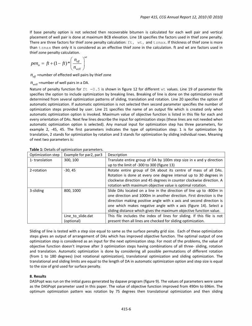
dapave program generates the initial input for optimization. A group of DAs are generated with no spacing between them. Figure 9 shows one of the arrangements of DAs generated by dapave program. The parameter file for dapave is:

Line START OF PARAMETERS: 1 cliped_realz10.out input realization file2 10 Number of realizations3 1 0 column number for variable, minimum4 1.0 minimum average for selection5 0.95 minimum fraction in grid6 100 50 100 nx, xmn, xsz


415‐4

7 100 50 100 ny, ysz, ymn8 5025 6145 origin of a DA9 0 azimuth of DA centerline10 1000 800 Length and Width of DA11 dapave.csv output DA file12 0 clip by polygon13 14

6666 9486 4466 9406 2880 7846 1880 7780

Number of vertices

…… …… Line 1 specifies the input realization file for primary variable (NCB). The name of input realization file is optional. If file is present then program calculates the average NCB value for each DA over all realization. Number of realization is indicated in line 2. Line 3 indicates the column number for primary variable and a minimum value pmin of primary variable used in calculation. A value less than pmin is included in the calculation by making it equal to pmin. A pmin value equal to 0 can be used to eliminate ‐999 values from the calculation. This way the average of primary variable over any DA doesn’t become negative. Line 3 specifies the minimum cutoff value of mean of primary variable over a DA. A DA with less value than cutoff value is not included in the DA arrangement. This option is helpful when one or more DAs are already present in the development area and any DA overlapping existing DA is not included in the configuration. It is also helpful to limit the number of DAs outside the development area. Line 5 specifies the cutoff value for fraction of DA area inside grid limits. Any DA having less than cutoff fraction area inside grid boundary is not included in the layout of DAs. This option is used to limit the number of DAs within the grid limits. Grid definitions are mentioned in lines 6 and 7. To generate a layout of compact arrangement of DAs, the centre of any one DA is required. This centre is specified in line 8. Orientations of all DAs in the arrangement are same and this orientation is specified in line 9. Line 10 specifies the length and width of DA. Line 11 specifies the name of the output file which is a .csv file and can be viewed in excel sheet. The output file follows a specific format which is input for DASPopt program. All four vertices of DA, orientation of each DA, and center of DAs are written in the output file. Line 13 specifies the option to clip DA`s by a polygon. If the centre of a DA is outside the input polygon (from line 13 and after) then it is not included in the layout. The input layout of DA`s are shown in figure 9 for DAs of size 1000m x 800m. DAplt (a MatLab function) is used to

plot the output of dapave. Numbering of DAs is generated by dapave. The individual rows of layout are shown with the help of lines with. These lines are named by numbers from 1 to11. Name of lines can be used in the optimization program to provide an option to slide or freeze individual lines. Naming of DA’s are indicated at their centers. There are total 99 DAs inside the model area. Number of DAs can be limited with option to clip inside development area polygon. But it will have no effect on final optimization result. Additional calculation time in case of more DA is not a major issue in optimization program. Some DAs outside the development area are necessary to play with optimization program.

7. Optimization program‐ DASPopt The method of automatic and optional optimization is explained in Kumar and Deutsch (2010). The

necessity of Automatic optimization checks all the possible combinations of translation, rotation and sliding and selects the global maximum from them.

The parameter file for DASPopt is shown in the next page. Line 1 of parameter file specifies the well spacing (horizontal distance between two well pairs of a DA) and radius of surface pad. Circular shaped pads have been assumed. The value of SP penalty is important in the optimization. A SP is penalized with value 0 if any part overlaps with a cell which indicates the presence of surface obstruction. In this case value of objective function becomes 0 for corresponding DA. Line 2 specifies 3 parameters. First parameter is the ideal distance (in meters) of SP from its DA, second and third parameters are the distance tolerances by which a SP can be located away from its ideal position (figure‐ 10). The location of a SP with respect to DA can be in maximum 4 directions (figure 10). Line 3 in the parameter file has 4 options to include search direction. A value with 1 includes corresponding direction for SP allocation. First option corresponds to direction‐1, second option for direction‐2 , and so on. Line 3 specifies the input realization files for reservoir variables (NCB, GCB, Thief zone, and BCB). Line 5 and 6 specifies


415‐5

the number of realizations and column numbers for different variables. Input surface penalty map is optional and is specified in line 7. If surface penalty map is not present then program assumes no penalty over model area i.e. SP is possible anywhere within model area.

Line START OF PARAMETERS: 1 160 100 well spacing, pad radius2 350 50 50 Ideal distance of SP from DA, dis1, dis23 1 1 0 0 search direction for SP (1‐yes, 0‐no) for all 4 directions4 clipped_realz.dat input realization file5 10 number of realizations6 1 3 0 2 columns for NCB, BCB, TZ, and GCB7 sc.dat input surface penalty map (optional)8 1 column number for surface penalty9 400 12.5 25 nx, xmn, xsz of surface penalty map10 400 12.5 25 ny, ymn, ysz of surface penalty map11 dapave.csv input file with initial configuration of DA12 DASPreal.out output by realization and DA13 DASPsumm.out summary output file14 DASPopt.out output file with final result of optimization 15 100 50 100 nx, xmn, xsz of realizations16 100 50 100 ny, ymn, ysz of realizations17 0 0.5 penalize base(1‐yes, 0‐recoverable reserve calculation), f1018 0.6 0.5 0.5 ft, wt, tzmax for thief zone19 1 optimization by breaking lines20 1 3 automatic optimization (1‐yes, 0‐user specified), nopt 21 DASPobj.out output file with maximum obj. fun values (in auto optimization only)22 1 1000 100 ‐optimization by translation23 2 -45 45 ‐optimization by rotation24 3 -1000 1000 ‐optimization by sliding25 line_to_slide.dat Input file with which lines to slide

The program assigns a penalty value of 0 if a surface pad is outside model area. Therefore model area should be select in such a way that it provides necessary space for placement of SP for a DA inside the development area. Line 8 gives the column number of surface penalty value in the input penalty map file. Line 9 and 10 specifies the definition of grid for surface penalty map. Line 11 specifies the name of input file with initial guess to run optimization. An output file with value of objective function for each realization is specified in line 12. File for output summary is mentioned in line 13. This file keeps records of objective function for each and every optimization steps. In case of automatic optimization summary file records all possible combinations of optimization patterns. Line 14 specifies the name of final output file. This s the main output file with optimal locations of DA, objective function value of each DA along with different penalty factors, recoverable reserve from each well pair and maximum BCB elevation along well pair. Line 15 and 16 specifies the grid definition for realizations of reservoir variables. Line 17 has 2 parameters related with base penalty. First parameter is flag for penalizing the base by including base penalty factor. Second parameter is f10 factor for base penalty calculation. Figure 11 illustrates the effect of f10 factor on nature of penalty function. avgd is calculated as:

1

1

ncell

i bcbicell

ncell

bcb iicell

iavgd bcb m

n

im bcb

n

celln =total number of cells inside DA. Value of base penalty is related with avgd by:

1 (1 10)* /10basepen f avgd


415‐6

If base penalty option is not selected then recoverable bitumen is calculated for each well pair and vertical placement of well pair is done at maximum BCB elevation. Line 18 specifies the factors used in thief zone penalty. There are three factors for thief zone penalty calculation: ft, wt, and tzmax. If thickness of thief zone is more

than tzmax then only it is considered as an effective thief zone in the calculation. ft and wt are factors used in thief zone penalty calculation.

(1 )*wt

efftz

well

npen ft ft

n

effn =number of effected well pairs by thief zone

welln =number of well pairs in a DA.

Nature of penalty function for ft =0.5 is shown in figure 12 for different wt values. Line 19 of parameter file specifies the option to include optimization by breaking lines. Breaking of line is done on the optimization result determined from several optimization patterns of sliding, translation and rotation. Line 20 specifies the option of automatic optimization. If automatic optimization is not selected then second parameter specifies the number of optimization steps provided by user. Line 21 specifies the name of an output file which is created only when automatic optimization option is invoked. Maximum value of objective function is listed in this file for each and every orientation of DAs. Next few lines describe the input for optimization steps (these lines are not needed when automatic optimization option is selected). Any manual input for optimization step has three parameters, for example 2, ‐45, 45. The first parameters indicates the type of optimization step: 1 is for optimization by translation, 2 stands for optimization by rotation and 3 stands for optimization by sliding individual rows. Meaning of next two parameters is: Table 1: Details of optimization parameters.

Optimization step Example for par2, par3 Description

1‐ translation 300, 100 Translate entire group of DA by 100m step size in x and y directionup to the limit of ‐300 to 300 (figure 13)

2‐rotation ‐30, 45 Rotate entire group of DA about its centre of mass of all DAs. Rotation is done at every one degree interval up to 30 degrees in clockwise direction and 45 degrees in counter clockwise direction. A rotation with maximum objective value is optimal rotation.

3‐sliding

800, 1000 Slide DAs located on a line in the direction of line up to ‐800m in one direction and 1000m in another direction. First direction is the direction making positive angle with x axis and second direction is one which makes negative angle with x axis (figure 14). Select a sliding distance which gives the maximum objective function value.

Line_to_slide.dat (optional)

This file includes the index of lines for sliding. If this file is not present then all lines are checked for sliding optimization.

Sliding of line is tested with a step size equal to same as the surface penalty grid size. Each of these optimization steps gives an output of arrangement of DAs which has improved objective function. The optimal output of one optimization step is considered as an input for the next optimization step. For most of the problems, the value of objective function doesn’t improve after 3 optimization steps having combinations of all three‐ sliding, rotation and translation. Automatic optimization is done by considering all possible permutations of different rotation (from 1 to 180 degrees) (not rotational optimization), translational optimization and sliding optimization. The translational and sliding limits are equal to the length of DA in automatic optimization option and step size is equal to the size of grid used for surface penalty.

8. Results DASPopt was run on the initial guess generated by dapave program (figure 9). The values of parameters were same as the DASPopt parameter used in this paper. The value of objective function improved from 490m to 696m. The optimum optimization pattern was rotation by 75 degrees then translational optimization and then sliding


415‐7

optimization. After breaking optimization final value of objective function was 707m. Figure 15 is showing optimum arrangements of DAs before and after breaking lines. The optimum value of objective function for every direction is shown in figure 16. The computational time for automatic optimization was less than 10 minutes on a computer with 2.00GHz processor and 3 GB memory. This time seems reasonable when working with almost 100 DAs, over 10 geological realizations and doing computation over a resolution of 400 x 400 for SP allocations.

References McLennan, J.A., Ren, W., Leuangthong, O., and Deutsch, C.V., 2006, Optimization of SAGD Well Elevation, Natural Resource Research, 15(2), 120‐121pp. Dowsland, K.A., Vaid, S.,Dowsland, W.B., 2002, An algorithm for polygon placement using a bottom‐left strategy, European Journal of Operational Research, 141, 371‐381. Babu, A.R., Babu, N.R., 2001, A genetic approach for nesting 2‐D parts in 2‐D sheets using genetic and heuristic algorithms, Computer‐Aided Design 33, 879‐891. Deutsch, C.V. and McLennan, J.A., 2005, Guide to SAGD (Steam Assisted Gravity Drainage) reservoir characterization Using Geostatistics Centre of Computational Geostatistics, Guidebook Series, Vol3. 2006, Athabasca, Husky Energy, Sunrise project, Resource Management Report, ERCB, Canada, 10419, 36pp. 2009, Athabasca, Encana, Christiana Lake project, Resource Management Report, ERCB, Canada, 8591, 142pp. Kumar, A. and Deutsch, C.V., 2010, Optimal Drainage Area and Surface Pad Positioning, CCG report, 202


415‐8

Figures

Figure 1: Clockwise from top left: An example of bitumen deposit to illustrate the necessity of optimization; placing first well‐ A at a location which gives maximum recovery for A; then placing well B at a location which gives maximum recovery for B; Not an optimal location for well A but the combined recovery is maximum.

Figure 2: Future plans for Drainage area locations. Christina Lake project, Encana, 2009 (left); Sunrise project, Husky Energy, 2006 (right); Taken from RMR reports, Canada.


415‐9

Figure 3: Reservoir variables‐ NCB, BCB, GCB, and TCB

Figure 4: One of the realizations of reservoir variables: NCB, GCB and BCB. Development area for the placement of DAs is shown on NCB map.

Figure 5: Surface obstruction over development area.


415‐10

Figure 6: Format of input file for setpen. All entity types are present in this file: 1 for polygon, 2 for line, 3 for arc and 4 for circle.

Figure 7: Surface penalty map at 25m x 25m grid size. Black areas are penalized.

Figure 8: Clipped NCB inside development area.


415‐11

Figure 9: Initial guess for optimization.

Figure 10: distance tolerances for SP location search (left). Direction of SP location with respect to a DA (right).


415‐12

Figure 11: Penalty function for base

Figure 12: penalty function for thief zone for ft = 0.5.

0 10 20 30 40 500

0.2

0.4

0.6

0.8

1

avgd

Pen

alty

Effect of f10 factor on base penalty

f10 = 0.95f10 = 0.05f10 = 0.25f10 = 0.5


415‐13

Figure 13: Optimization by translation: par1 =1, par2 =300, par3=100. Input for translational optimization (left). A is a reference point for arrangement. Value of objective function is checked by moving A (entire arrangement) at all intersection points of horizontal and vertical lines (right). One such test is shown. A location with maximum objective function is selected at the end as an optimum translation.

Figure 14: Sliding optimization of individual rows. Definition of direction of a line.


415‐14

Figure 15: Optimal locations of DA and at 165 degrees orientation of DA centerline (left). Optimization after breaking lines (right).

Figure 16: maximum value of objective function for different orientations.

Documents

Program for SAGD Drainage Area and Surface Pad … for SAGD Drainage Area and Surface Pad ... data by a polygon, dapave program generates ... Generally, clipping outside a polygon