Embed Size (px)
Citation preview

0
Profitability and Stock Returns in Production-Based Asset Pricing with Decreasing Returns to Scale *
Ronald J. Balvers
DeGroote School of Business McMaster University
Email: [email protected]
Li Gu Division of Banking Supervision and Regulation
Federal Reserve Board Email: [email protected]
Dayong Huang
Bryan School of Business and Economics University of North Carolina at Greensboro
Email: [email protected]
January 10, 2014
Abstract
In a production-based asset pricing model with decreasing returns to scale following Brock (1982) stock returns at the firm level no longer identically equal investment returns but, instead, are determined by a measure of gross profitability, the book-to-market ratio, and the change in future profitability prospects. Firm decisions of capital investment and utilization both negatively predict profitability and future returns. Book-to-market ratios positively forecast returns as is typical, but with specific predicted exceptions. These implications are confirmed empirically and the production-based model with decreasing returns predicts costs of equity capital better than traditional asset pricing models. JEL Classification: G12. Keywords: Profitability; Stock returns; Production-based asset pricing; Investment returns; Capacity utilization; Decreasing returns to scale * We thank Andrew Ang, Ujjal Chatterjee, Ilan Cooper, Zhi Da, Fanchang Huang, Januj Juneja, Xiaoji Lin, Jianjun Miao, Yangru Wu, Hayong Yun, and seminar participants at the Central University of Finance and Economics, Fordham University, McMaster University, the Federal Reserve Bank at Richmond, and the FMA annual meeting in Chicago for valuable comments.

1
Profitability and Stock Returns in Production-Based Asset Pricing with Decreasing Returns to Scale
1. Introduction
We modify the investment-based asset pricing approach of Cochrane (1991, 1996) by
building directly on the formulation of Brock (1982) which models capital accumulation on a
time-to-build assumption rather than adjustment costs and assumes decreasing returns to scale
instead of constant returns. The assumption of decreasing returns allows us to highlight the role
of profitability on equity returns and substantially modifies Cochrane’s investment-based
approach because unlevered stock returns no longer equal investment returns. Investment returns
still explain stock returns but only partially: we derive that stock returns are a weighted average
of average investment returns (including a profitability markup) and the rate of change in the
value of intangible assets, with weights related to the book-to-market ratio. A significant
implication of this result is that it captures theoretically the dual aspects of value documented
empirically by Novy-Marx (2013): profitability and the book-to-market ratio have separate
positive effects on required stock returns.1
Allowing decreasing returns to scale also lets us move away from the convex adjustment
costs formulation that has dominated investment-based asset pricing research. While convex
1 These outcomes may suggest the naïve perspective that the best way to invest is by purchasing “cheap” (high book-to-market) stocks in “good” (high profit rate) companies. However, predictability of stock returns arises here in an efficient market. The positive return impact of book-to-market ratios is a result of tangible asset values being more sensitive than intangible asset values to mean-reverting productivity shocks, and the positive effect of profitability on returns stems from firms becoming more profitable as a reward for having chosen the riskier production route (as in Berk, Green, and Naik, 1999).

2
adjustment costs are analytically convenient and are helpful in allowing the model to numerically
replicate asset price variability and investment dynamics (Jermann, 1998, and Zhang, 2005), they
are hard to rationalize as a uniform vital source of economic dynamics. Hall (2004) argues that
convex adjustment costs of investment are too small to explain large fluctuations in stock prices.
Abel and Eberly (2011) show that a model without adjustment costs can explain both the low
sensitivity of investment to the book-to-market ratio and the higher sensitivity of investment to
operating profit, which are hard to explain with convex adjustment costs. And the survey by
Caballero (1999) makes it clear that investment choices are influenced by convex adjustment
costs in some firm-level environments, but by non-convex adjustment costs in others. Convex
adjustment costs thus may provide a confounding basis for understanding differences in firm-
level investment returns, even if adequate at the aggregate level.2 The recent work of Bloom
(2009), Lin and Zhang (2013), and Belo, Bazdresch and Lin (2013) considers both non-convex
and convex adjustment costs in investment and makes progress in replicating firm-level
investment dynamics. It, however, relies heavily on numerical methods.
On the other hand, our productivity-based formulation maintains the important strengths
of the investment-based formulation.3 Firms in effect choose the riskiness of their operations,
2 The adjustment cost assumption has been popular in part because it can account for more variability in investment returns and accordingly higher asset price volatility. In our time-to-build framework, however, profitability factors unrelated to investment returns also affect stock prices and these may be highly variable, especially since we interpret the productivity shocks that drive profitability more broadly than total factor productivity. It is not our intent here to calibrate a general equilibrium model to explain the size of the equity premium or match the volatility of asset prices. Remaining outside the confines of the standard real business cycle model, and avoiding explanations that rely on time-series variation in risk premia, we see no a priori reason that our model would have trouble explaining asset price volatility.
3 To streamline terminology we propose to refer to Brock’s (1982) contribution as productivity-based asset pricing and to Cochrane’s (1991) contribution as investment-based asset pricing. Both are special cases of production-based

3
and observed internal decisions provide a real and current signal as to management’s information
and intended level of risk exposure. A firm’s chosen characteristics provide a timely and
accurate measure of risk sensitivities perceived by insiders. As Lin and Zhang (2013)
emphasize, it is the promise of investment-based, and more generally production-based asset
pricing, to identify the links between production decisions and risk exposure such as to provide
estimates of costs of capital that are more precise than those derived from the traditional
consumption-based approach. The consumption perspective requires that risk loadings be
estimated from past time series of returns with or without ad-hoc conditioning variables; the
production perspective determines the structural variables that drive the risk loadings. Lin and
Zhang (2013) argue that the production-based view may well turn out to provide superior
estimates of costs of capital, with the potential of a paradigm shift in asset pricing.
Several recent papers also relate profitability and stock returns, using elements of the
Brock approach. Li, Livdan, and Zhang (2009) present a hybrid of Brock’s productivity-based
approach and Cochrane’s investment-based approach by allowing both decreasing returns to
asset pricing which focuses on the production side rather than the traditional consumption side to derive implications for asset returns. Production-based asset pricing as broadly interpreted builds on the theoretical work of Brock (1982), Cox, Ingersoll, and Ross (1985), and Berk, Green, and Naik (1999) and has been applied to explain and predict stock returns by Balvers, Cosimano, and McDonald (1990), Hsu (2006), Balvers and Huang (2007), Booth et al. (2008), Lioui and Poncet (2008), Kogan and Papanikolaou (2012, 2013), and others. Brock (1982) assumes production under a decreasing-returns-to-scale technology with time to build and an array of productivity shocks driving firm decisions. Stock returns here depend on production decisions that interact with the firm’s exposure to the various productivity shocks. Cochrane (1991) and Restoy and Rockinger (1994), building on the q-theory of Tobin (1969) and Hayashi (1982), show that stock returns are identical to investment returns in an environment with constant returns to scale and convex adjustment costs, thus summarizing the production attributes relevant for determining stock returns as simply the determinants of investment returns. This investment-based approach to asset pricing has stimulated a growing body of empirical work by Cochrane (1996), Gomes, Kogan, and Zhang (2003), Carlson, Fisher, and Giammarino (2004), Zhang (2005), Xing (2008), Liu, Whited and Zhang (2009), Li and Zhang (2010), Hou, Xue, and Zhang (2012), Lin and Zhang (2013), and others.

4
scale and convex adjustment costs. Although they succeed in explaining external financing
anomalies, they additionally contend that stock returns and profitability (equal to cash flows in
their model) are inversely related. This is counter factual in light of Novy-Marx’s (2013)
findings and reverses the result we obtain in the pure Brock framework. Since the results are
largely numerical it is challenging to identify the exact mechanism, but Li et al. (2009) argue
along the lines of the pure investment-based approach that higher profitability facilitates
investment, and that, in turn, higher investment implies lower investment returns and stock
returns. Empirically, Li et al. support this prediction by identifying a positive interaction effect
between profit (cash flows) and investment, which affects returns in addition to the investment
link by itself. However, they do not control for the effect of profitability by itself which likely
accounts for the discrepancy between their findings and those of Novy-Marx.
The work of Kogan and Papanikolaou (2012, 2013) may be viewed as a structural version
of the Brock approach with two types of productivity shocks. By adding a second, investment-
specific, productivity shock to traditional approaches (such as Jermann, 1998, Boldrin,
Christiano, and Fisher, 2000, and Balvers and Huang, 2007), they generate additional
implications and avoid relying on the Solow residual to operationalize productivity shocks.
Their model produces a positive link between returns and both book-to-market ratios and
profitability: higher growth options imply more exposure to investment-specific technology
shocks that mitigate market risk, causing lower average stock returns; and higher profitability
implies riskier tangible assets and more exposure to total factor productivity shocks, causing
higher average stock returns. By explaining the dual dimensions of value and by avoiding the
empirical use of Solow residuals, Kogan and Papanikolaou attain some of the key objectives of

5
our paper. However, our paper offers a substantially different perspective: illustrating alternate
economic mechanisms and correlations, producing distinct new testable implications, generating
cost of capital predictions without requiring time series estimation of factor betas, and providing
a simple model with closed-form solutions for profitability rates, book-to-market ratios,
investment returns, stock prices and stock returns.
We add a utilization decision to the Brock model to generate a richer decision
environment that is more revealing about the information available to management.4 Investment
takes time to become productive, but adjusting utilization is instantaneously productive. Both
decisions convey important, distinct clues about the firm’s sensitivity to risk. Risk arises as a
result of persistent productivity shocks which we interpret not in the narrow sense of technology
shocks but, as in Novy-Marx (2013), more broadly as profitability shocks affecting individual
firms through exogenous changes in, for instance, total factor productivity, market conditions,
competitiveness, the macro environment, and input costs.
The model generates closed-form solutions for stock returns, profitability, book-to-
market ratios, investment, and the utilization rate that provide new testable implications. First, in
addition to the standard implication that investment as a signal of future productivity affects
expected stock returns, utilization as a signal of perceived current productivity also affects
expected returns. Both are inversely related to expected profitability and expected stock returns.
4 There are investment-based asset pricing papers that also provide a richer decision environment. In particular, Chen and Zhang (2011) explicitly consider employment as an additional input factor affecting investment returns and hence future stock returns. They look at aggregate inputs only. Employment, furthermore, has the drawback of being very heterogeneous. It is important to distinguish between hours worked per person and the number of persons employed; distinguish between skilled and unskilled; and consider the impact of labor hoarding. In contrast, capacity utilization, as we capture it by electricity usage, is a more homogeneous measure of activity.
6
Second, a higher current book-to-market ratio normally (i.e., unconditionally) indicates higher
future returns, the standard value effect, because the higher book-to-market ratio implies more
weight on the tangible value component, which has higher average returns, and less weight on
the intangible value component, which has lower average returns.5 But, in specific instances –
whenever intangible asset returns are expected to exceed tangible asset returns – the model
implies that the book-to-market effect does not hold and is, in fact, reversed as we confirm
empirically.
The implied impact of investment and utilization on future stock returns is tested using
the Manufacturing Industry Database, made available by the National Bureau of Economic
Research and the Center of Economic Studies (NBER-CES), in combination with
COMPUSTAT. The Manufacturing Industry Database provides industry-level historical data for
459 industries on the stock of physical capital, spending on electricity, and productivity. This
database has not been applied extensively in this context (Booth et al. 2008 is the exception) but
is well suited for our purposes. Electricity usage per unit of capital provides a desirable proxy for
the utilization rate that appears to be a more reliable indicator of the intensity of usage of the
firm’s production capacity than reported utilization rates. We merge industry-level electricity
expenditure deflated by the price index for electricity per unit of capital with the COMPUSTAT
5 Technically, we show that the risk-adjusted returns on tangible capital must follow a submartingale process, while the risk-adjusted returns on intangible capital must follow a supermartingale process.

7
firms by SIC code and assume that COMPUSTAT firms in the same industry have similar
utilization rates. 6
The empirical results support the model predictions. We find that both the investment-to-
capital ratio and the utilization rate have significant negative forecast power for returns.7 In
addition, the book-to-market ratio has the expected positive return effect for the average firm, but
as predicted explicitly, is reversed in cases for which returns on intangible assets are expected to
exceed returns on tangible assets. We further find that prediction of the cost of capital from our
production-based model works significantly better than prediction of the cost of capital based on
the CAPM or the Fama-French three-factor model.
2. Production, Profitability, and Expected Stock Returns
We present first an equilibrium model along the lines of Brock (1982), Cox, Ingersoll,
and Ross (1985), and Berk, Green, and Naik (1999), that allows prediction of the required return
on the equity of a particular firm from market conditions and firm characteristics, utilizing a
production-side perspective. The model makes explicit the impact of decreasing returns, and the
associated capital investment and utilization decisions, on expected returns and profitability. The
6 Burnside, Eichenbaum, and Rebelo (1995) originally used electricity usage as a proxy for capacity utilization. Da and Yun (2010) employ electricity consumption in the asset pricing context. They approach this issue from a consumption-based asset pricing perspective, viewing electricity consumption as a high-frequency alternative measuring consumption in real time.
7 The evidence that investment is negatively related to future returns is consistent with, for example, Cochrane (1991, 1996), Titman, Wei and Xie (2004), Zhang (2005), and Xing (2008).

8
impact is time-varying and suggests predictability of realized stock returns based on prior
profitability, value, utilization and investment information.
Firm decisions with capital, capital services, and decreasing returns
Consider a representative firm maximizing the expected net present value to shareholders with
respect to its production and investment choices in each period. The maximized value of the
firm V is determined as the present value of dividends to the shareholders:
( ))],([),( 111,
++++= tttttIU
tt KVmEDMaxKVtt
θθ , (1)
which is the standard Bellman Equation of dynamic programming. The dividends paid by the
firm in each period t are denoted by tD . The productivity variable tθ and the available capital
stock tK are the state variables which are jointly sufficient for determining firm value.8 The
aggregate stochastic discount factor is given as 1+tm , and )(⋅tE carries the subscript t to indicate
that expectations are conditional on all currently available information.
The maximum value of the firm ),( ttt KVV θ≡ is the equity value of the firm before
dividends: ttt DPV += , with )],([ 111 +++= ttttt KVmEP θ the ex-dividend equity value of the firm.
Given the definition of the stock return, ttttS
t PPPDr /)( 111 −+= +++ , equation (1) can be rewritten
as )]1([1 11S
ttt rmE ++ += , reflecting the fact that risk- and dividend-adjusted stock prices follow a
8 It is clear from the specification in equations (1) - (4) that, indeed, the productivity variable θt and the available capital stock Kt are sufficient state variables for the value of the firm

9
martingale process so that pricing the equity value of the firm according to equation (1) rules out
arbitrage opportunities.
We assume that net operating income, tY , is determined by a simple power function of
the firm’s current physical capital stock, tK , the choice of the utilization of its currently
available capital stock, tU , and by the exogenous current level of productivity, tθ :
βααθ tttt KUY −= 1 .9 Dividends tD are then given as:
ttttt IqKUD −= − βααθ 1 , (2)
with tI the current level of capital investment and q the relative price of an investment good. For
later use we define ttt KUu /= as the fraction of the capital stock chosen to be utilized for
current production, and ttt KIi /= as the current level of investment per unit of capital that will
contribute to next period’s capital stock.
Productivity tθ here is to be interpreted quite generally. It is a conflation of technology
shocks and other disembodied productivity shocks together with miscellaneous exogenous
factors that affect the profitability of the firm, such as changes in the competitive environment,
and input costs (see, e.g., Novy-Marx, 2013, for a similar characterization of productivity).
Following Brock (1982) we may view tθ as a vector containing a multitude of systematic
productivity shocks. We choose not to do so formally to keep the notation simple and because
9 The exponent on the productivity level in the production function is similar to that in Cooper (2006). Abel and Eberly (2011, equation 3) show that this specification naturally arises given our interpretation of Yt as revenue net of labor cost.

10
this generalization would add few new insights given our focus. However, we note that a multi-
productivity-factor version would be easy to deal with in our production-based approach while
making it difficult to apply the CAPM.
The interpretation of tY as operating income means that we have implicitly accounted for
the impact of labor and additional inputs on production and costs, which are only represented by
the exogenous influence of wages and other input costs on income, captured by the productivity
level tθ . Capital is viewed as productive even if not in use, so we take 0>β . The reason is that
excess capacity on average, while not continuously in use during a period, nevertheless allows
for better maneuverability, increased flexibility, and a frictionless way of dealing with peak load
scenarios and fluctuating demand. We also set 0>α and assume decreasing returns to scale so
that 1<+ βα . In this we follow Brock (1982) but differ from Cochrane (1991) and others in the
investment-based asset pricing literature, with the critical implication that investment returns are
distinct from stock returns. We express the degree of decreasing returns to scale as
0/)1( >−−= ββαs so that higher s represents stronger decreasing returns to scale and higher
profitability.
We next specify the equations of motion for the state variables. Capital evolves
according to the standard linear specification but with the refinement that depreciation depends
in part on usage as is emphasized by McGrattan and Schmitz (1999):
tttt IUKK +−−=+ γδ )1(1 (3)
Capital increases with existing capital and investment, and decreases in the intensity of its
current utilization. The rate of deprecation becomes equal to tuγδ + . We interpret investment
11
broadly to include changes in working capital so that, under clean surplus accounting, capital
becomes conceptually equal to total assets and the book value of the firm.
The exogenous productivity indicator follows a linear Markov process:
111 )1( +++ +++−= tttt ησερθθρθ , (4)
Where tη is a firm-specific i.i.d. random variable with arbitrary distribution that has mean zero
and variance 2ησ , and tε is an aggregate i.i.d. variable, tε , with an arbitrary distribution that is
standardized to have zero mean and unit variance, and is independent of tη . The autoregressive
formulation for productivity is inherited by the process for profitability (although inversely) and
captures two features of the data: persistence of profitability and mean reversion of profitability
at the firm level (Fama and French, 2000 and 2006).
The aggregate shock tε is the only systematic risk (although we could with minor
complications model a vector of such systematic productivity shocks as in Brock, 1982) and we
specify the stochastic discount factor exogenously as
r
hm t
t +−=1
1 ε. (5)
It follows that rmE tt +=+ 1)/(1 1 so that r represents a constant risk free rate; h is the constant risk
premium of the systematic productivity risk. The stochastic discount factor parameters h and r ,
together with the price of investment goods q, are the only aggregate parameters in the model.
All other parameters may differ across firms. The exogenous stochastic discount factor is in the
tradition of Berk, Green, and Naik (1999) and allows us to focus on differences in factor risk

12
sensitivities of individual firms as determinants of returns, while taking the aggregate values for
the risk free rate and the risk premium as given.
Optimal investment and utilization
Maximization of the value of the firm in equation (1), subject to equations (2), (3), and
(4) with respect to investment and capacity utilization, yields the first-order conditions for the
investment choice (barring time subscript t, all subscripts indicate partial derivatives):
)],([ 111 +++= ttKtt KVmEq θ , (6)
and for the capacity utilization choice:
)],([ 11111
+++−− = ttKttttt KVmEKU θγθα βαα . (7)
The first-order conditions together immediately yield a solution for optimal capital utilization:
αβ
α θγα −−= 111
)/(*ttt KqU . (8)
The optimal capital stock is subsequently found in Appendix A as
βαα
ρθ −−−
+=+1
1
)]([*1 tt zAK , with )(/)/( 1 δγαβ α
α
+≡ − rqqA , σθρ hz −−≡ )1( . (9)
Optimal investment *tI may be inferred directly from equations (3), (8) and (9).
3. Implications
The model solutions allow us to relate stock returns to investment returns, profitability
measures, and value measures, providing several new testable implications in the process.

13
Investment returns and stock returns
In equation (6), )],([ 111 +++= ttKtt KVmEq θ , which implies that the investment return
qqKVr ttKI
t /]),([ 111 −≡ +++ θ can be viewed as a regular asset return because 1)]1([ 11 =+ ++I
ttt rmE .
The excess investment return is derived straightforwardly in Appendix A:
)()( 11
1 δθρ
ηεσ +
+
++=− +++ r
z
hrr
t
ttIt . (10)
The expected excess investment return equals )/()(1 tI
tt zhrrrE θρσδ ++=−+ .
In the constant returns to scale (CRTS) framework of Cochrane (1991, 1996) the
marginal investment return equals the average investment return which in turn equals the stock
return: St
It rr 11 ++ = . But in our decreasing returns (DRTS) model the two are not identical and a
comparison is instructive. Compare qKVr ttKI
t /),(1 111 +++ ≡+ θ and tttS
t PKVr /),(1 111 +++ ≡+ θ .
Under CRTS (with or without adjustment cost) it is necessarily true that both
11111 /),(),( +++++ = tttttK KKVKV θθ and 1+= tt KqP where, in the case of adjustment costs, q
represents the full price of a capital good – the cost of purchasing and installing the capital good.
It follows then that St
It rr 11 ++ = .
Under DRTS there are two sources of difference because (a) average returns to capital
and marginal returns to capital differ, qKVqKKV ttKttt /),(/),( 11111 +++++ ≠ θθ , and because (b) book-
to-market values are not one: 1/1 ≠= + ttt PKqb implying tttttt PKVqKKV /),(/),( 11111 +++++ ≠ θθ . As
shown in Appendix B and as also consistent with Abel and Eberly (2011) in a related framework
(but focusing on investment rather than asset prices): tb in this model is always lower than one,

14
1/1 <= + ttt PKqb , because the firm has a strictly positive intangible asset value (in spite of not
facing adjustment costs).10 Thus, variations in the scale of the firm and in the book-to-market
value of the firm cause stock returns to deviate from investment returns. These differences are
intriguing because they correspond to the well-documented size and value effects, respectively.
Appendix B derives an expression for stock returns in relation to investment returns:
)1(111 ttttS
t bgbr −+= +++ π , )( δπ ++≡ It
Itt rsr . (11)
The book-to-market ratio PKqbb ttt /)( 1+== θ represents a predetermined weight 10 << tb ,
and ),( 11 ttt gg θθ ++ = is the rate of increase in the firm’s intangible asset value. We obtain the
average investment return as )( δπ ++= It
Itt rsr which equals the marginal return on
investment Itr (stated in equation 10) plus a markup that results from decreasing returns to scale.
Abel and Eberly (2011, equation 3) show that, in a formally identical model, the markup can also
be interpreted as the profit arising from market power. The markup here is the product of the
degree of decreasing returns, ββα /)1( −−=s , and the appropriate user cost of investment,
which equals the investment return (the risk free rate plus a compensation for investment risk),
plus the depreciation rate, δ+Itr . Essentially stock returns are a weighted average of the return
on tangible assets (the average investment return) and the return on intangible assets (the rate of
increase in the value of growth options) with the weights equal to tb and tb−1 . Note that both
10 The intangible asset value is the expected present value of future streams of residual income. The residual income is the abnormal profit, the net income after adjusting for the opportunity cost of capital, and here arises exclusively from the profit markup caused by decreasing returns to scale.

15
the mean value and the risk of the average investment return increase directly in the degree of
decreasing returns to scale, s.
The intuition for why unlevered stock returns deviate from investment returns is that
decreasing returns imply that the (marginal) investment return affecting real decisions is below
the average return paid out to stockholders; i.e., average investment returns are larger than
marginal investment returns. Additionally, even the average investment return is only the return
from tangible assets going to stockholders and should be weighted by the tangible part of total
equity value. Another part of the asset’s market value affecting stockholder returns derives from
profitability prospects. The change in the value of these “growth options” provides a second
component of the stock return, weighted by the share of intangible assets in total equity value.
In our model, profit margins and investment returns are high when investment exposes
the firm to high systematic risk. High profit margins thus proxy for high σ (see equation 10),
signifying high levels of systematic risk and high (productivity) betas.11
Profitability and stock returns
The average investment return can be interpreted as a profitability measure. Rearranging
the definition in equation (11), =+ δπ t ))(1( δ++ Itrs represents a gross return which is shown
in Appendix B to equal the gross profit of the firm as a fraction of the initial book value,
11 Hou, Xue, and Zhang (2012) argue that an investment-based model with an investment factor and a profitability factor in addition to the traditional market and size factor can explain a large variety of financial market anomalies. Their motivation for separate investment and profitability factors is based on a framework in which investment returns and stock returns are equal but they break up the investment return into parts depending on the return on equity and the investment-to-capital ratio. They treat these components as separate systematic risk factors rather than indicators of risk sensitivities.

16
=+ δπ t ttt qKUY /)( γ− , which equals operating income minus maintenance costs divided by
the book value of assets. It is similar in spirit to Novy-Marx’s measure of gross profitability,
although our theoretical model is not detailed enough to distinguish this measure from other
profitability measures such as the return on assets.12 Thus,
PROPOSITION 1. Given decreasing returns to scale technology, expected stock
returns increase in expected gross profitability: 0)(/)( 11 >=++ tttS
tt bdErdE π .
This follows directly from equation (11). Akin to the approach in Berk, Green, and Naik (1999),
higher profitability means that the firm is more sensitive to the risk of current productivity
shocks and therefore has higher expected return. For a given productivity level, the firm has
chosen riskier investment projects (higher σ) which imply higher profitability, from equation
(10), as well as higher expected return, from equation (11).
Novy-Marx (2013) finds that the gross profitability of firms – current revenue minus the
cost directly attributable to current revenue generation – provides another dimension of value
and has significant forecast power for returns that is separate from the traditional book-to-market
effect. Empirically he finds in double-sorting US firms from 1963-2010 that the monthly returns
between high and low profitability quintiles is 0.68% per month, averaged over all book-to-value
12 The model, however, is detailed enough to eliminate cash flow measures (such as Free Cash Flow) as a proxy for profitability in this context because the investment expenditures that must be subtracted to calculate cash flows are not subtracted here in deriving the average investment returns.

17
quintiles; and the monthly return between high and low book-to-market quintiles is 0.54%,
averaged over all profitability quintiles.
The effect of profitability on stock returns may also be related to the effect of operating
income on stock returns that Li, Livdan, and Zhang (2009) find numerically in their model and
confirm empirically. They employ the Brock model but add convex investment adjustment
costs. For given positive investment, they find that higher operating income relative to assets has
a negative impact on stock returns. This result appears to conflict with the empirical Novy-Marx
(2013) result and with our theoretical result, both implying a positive impact of operating income
on stock returns. The likely reason is that Li et al. (2009) consider only the interaction between
operating income and investment, and not operating income in isolation.
The modification from marginal investment returns to average investment returns in
linking to stock returns is analogous to the impact of operating leverage emphasized by Carlson,
Fisher, and Giammarino (2004) and Novy-Marx (2011), but here represents a profit markup
derived from the extent of the decreasing returns s measured by ββα −−1 , and has diametrically
opposed empirical implications. Novy-Marx (2013, p.16) points out that in existing models
(Carlson et al., 2004, Zhang, 2005, and Novy-Marx, 2011) operating leverage and risk, and
hence expected returns, are increasing in fixed costs. Therefore, since higher fixed costs lower
profits, expected returns are negatively linked with profitability, implying that profitable firms
should underperform unprofitable firms in the stock market. In our model, however, the
“operating” leverage arises directly from the inherent profit markup and is linked positively to
profitability and stock returns (though negatively to the productivity level).

18
Kogan and Papanikolaou (2013) also generate the observed positive correlation between
profitability and expected stock returns that we find in our model. The positive correlation arises
because firms that are currently more profitable have less of their value linked to future
investment and they are therefore less susceptible to investment-specific productivity shocks. In
turn, investment-specific productivity shocks are found to mitigate market risk so that highly
profitable firms are riskier. This intuition relies on highly profitable firms typically being value
firms and appears to be inconsistent with the negative correlation between profitability and book-
to-market ratios identified by Fama and French (1995).
Model predictions relating to the value effect
Separately, tb , the book-to-market ratio also affects the firm’s expected stock return. The
effect is positive and magnifies the profitability effect if the average investment return
)( δ++ It
It rsr exceeds the rate of increase in intangible assets 1+tg . This is highly likely since the
average return on tangible assets is generally strongly positive while the rate of increase in
intangible assets must be zero in the unconditional average because the productivity shocks are
stationary, and, in fact, should be negative after risk correction as we argue next.
The risk-adjusted stock price must follow a martingale process as is implied by
)]1([1 11S
ttt rmE ++ += . Remarkably, while the stock return in equation (11) is a convex
combination of the average investment return and the appreciation rate of intangible assets, it is
not true that the average investment return and the intangible asset appreciation rate follow
martingale processes. Because 1)]1([ 11 =+ ++I
ttt rmE it follows from )( 111 δπ ++= +++I
tI
tt rsr that

19
1)]1([ 11 >+ ++ ttt mE π for 0>s . In mathematical terms, the average investment value follows a
strict submartingale process. Accordingly, 1)]1([ 11 <+ ++ ttt gmE , so that risk-adjusted intangible
assets follow a strict supermartingale process (see Appendix B). The reason the value of
intangible assets (adjusted for risk and time value) is expected to decrease over time is that here
the intangible asset consists of the present value of future profit markup which produces profits
in the next period that are counted as part of the average investment payoff, not the intangible
asset payoff.13
The practical implication is that, in typical cases, value effects must be positive: in
equation (11) higher tb implies that stock return is higher by an extent related to the positive
difference between the returns on a submartingale and a supermartingale (which is positive in the
time series average). The value effect therefore arises because value stocks have more weight on
tangible returns which normally are larger than the growth rate of the intangible component. Our
model accordingly provides a direct explanation for the Novy-Marx results: the comprehensive
value returns stem from firm-level preferences for high-profit-margin production projects with
accompanying high exposure to systematic shocks, and the effect is magnified in “value” firms
that also have more tangible assets relative to intangibles assets.
Another implication of our theory, a further refinement of the value effect not tested by
Novy-Marx (2013), is that the standard book-to-market premium should be the opposite (i.e.,
13 The component of intangible assets that enhances the average investment return can alternatively be interpreted as the tangible return on the fixed factor (location, brand name, disembodied know how, plant specific human resources or management skills, etc.) responsible for decreasing returns.

20
negative) for the (presumably small) segment of firms that has rates of increase in intangible
assets expected to exceed the return on tangible assets (see Appendix B). For these firms an
increase in the book-to-market ratio, raising the weight on the tangible asset return, lowers the
overall stock return, causing an inverse value premium. Of course these firms would necessarily
have relatively low exposure to productivity risk in their tangible assets (assets in place)
compared to their intangible assets (present value of future residual income). In summary,
PROPOSITION 2. Book-to-market ratios affect expected stock returns (given
decreasing returns and for given profitability): )(/)( 111 +++ −= ttttS
tt gEdbrdE π .
The effect is (a) positive unconditionally: 0)()( 111 >=− +++ ttt EgE ππ , and (b)
negative only for particular firms with )()( 11 ++ > tttt EgE π , for which the increase
in intangible asset values is expected to exceed the return on tangible assets.
The result follows from equation (11) and because tθ and, so intangible value )( tG θ , is
stationary, causing )( 1+tgE , the unconditional growth rate of )( tG θ , to be zero (see Appendix B).
A higher book-to-market ratio implies a higher expected return because, with more
tangible assets, a current productivity shock has a larger impact on market value. The reason is
that tangible assets benefit directly from the shock, whereas intangible assets capitalize the future
impact on profit which diminishes due to the mean reversion of tθ assumed in equation (4). In
particular cases, higher book-to-market values lower expected excess returns. Namely, for the
subset of firms that have expected rates of increase in intangible assets higher than their expected
average investment returns, an increase in tb implies less risk and lower expected stock returns.

21
Our economic argument for why value firms have higher average returns is different
from that in the existing literature. Zhang (2005) argues that value firms are riskier because they
are stuck with high (convex) adjustment costs when marginal utility is high. Cooper (2006)
assuming non-convex adjustment costs argues that value firms are riskier because they can
expand costlessly and benefit more strongly from positive shocks when their production capacity
is high. Both arguments hinge on adjustment costs and the conditional variation of risk premia,
which we avoid. The explanation of Kogan and Papanikolaou (2013) avoids both adjustment
costs and conditional variation of risk premia and holds that growth firms are more susceptible to
investment-specific productivity shocks which have negative risk premia (under plausible
assumptions). These explanations are not mutually exclusive and, in principle, each could
contribute to explaining the value premium.
Novy-Marx (2013) finds that the traditional value effect is not merely separate from the
profitability effect, but is in fact enhanced when he controls for profitability. Kogan and
Papanikolaou (2013) also confirm this observation which their model can match quantitatively
even though book-to-market ratios and profitability rates are positively correlated in their model.
Our model generates the same result stemming from the fact that book-to-market ratios and
profitability rates are negatively correlated in our model as is consistent with Fama and French
(1995). The negative correlation arises from a higher productivity level implying both a lower
profitability rate (more capital lowers the average return on capital) and a higher book-to-market
ratio (current productivity boosts raise tangible asset values more than intangible asset values
due to mean reversion). The negative correlation between book-to-market ratios and profitability

22
rates means that a high profit rate, for instance in part due to high σ and in part due to low tθ , is
associated with a lower book-to-market ratio which partly or fully offsets the effect of the profit
rate on stock returns. Sorting by book-to-market ratio in addition to profitability, avoids the
cases in which profitability is high for reasons having relatively small impact on expected returns
(low tθ for instance), implying a larger profitability premium when portfolios are double sorted.
Productivity and stock returns
Higher current productivity tθ at a particular firm forecasts lower expected stock returns
)( 1s
tt rE + for a given book-to-market ratio. This follows from equation (11) since both tangible
and intangible asset returns are expected to drop when the productivity level rises. Regarding the
tangible asset return, 0/)( 1 <+ ttt ddE θπ as follows because =++ δπ 1t ))(1( 1 δ++ +I
trs and
)/()(1 tI
tt zhrrrE θρσδ ++=−+ . The expected investment return is lower because the marginal
value of capital is lower at the higher capital level chosen in response to a higher productivity
level. Furthermore, 0/)( 1 <+ ttt dgdE θ resulting from the mean reverting process for tθ .
The current productivity level tθ is positively related to the proportional level of
investment ttt KIi /= : from equations (A3) and (9), the new capital stock is directly related to
)( 11 ++ ttt mE θ and thus depends positively on current productivity as well. It is also positively
related to the utilization rate ttt KUu /= : from equation (8) tu is proportional to tθ . Both
investment and utilization provide distinct information about productivity which is important
because productivity itself cannot be observed directly and in practice is typically measured as

23
the Solow residual. 14 By employing investment and utilization we bypass using the Solow
residual. Utilization helps pin down the current state of productivity, and investment helps pin
down the level of productivity expected in future periods, both of which help to predict next
period’s productivity level.
Equations (8) and (9) together with the capital accumulation equation (3) to determine
investment relate both ttt KIi /= and ttt KUu /= to the two state variables tθ and tK . By the
implicit function theorem we can solve for ),( ttt uiθθ = and ),( ttt uiKK = . Thus, we may replace
productivity tθ by two instruments tu and ti that jointly perfectly describe it. Furthermore, we
know that, conditionally on tb , 0/)( 1 <+ ts
tt drdE θ . Thus,
PROPOSITION 3. The level of productivity negatively affects expected stock
returns conditional on the book-to-market ratio: 0/)|( 1 <+ tts
tt dbrdE θ (given
decreasing returns). Without loss of information, tθ may be replaced by
),( ttt uiθθ = so that (a) 0/),|( 1 <+ ttts
tt diubrdE , and (b) 0/),|( 1 <+ ttts
tt duibrdE .
The cost of capital
The single systematic factor in the model implies theoretically that any conditional one-
factor model, such as a conditional version of the CAPM, must apply equally well as our
14 Given our broader interpretation of productivity shocks and the complications of its measurement in the presence of changes in utilization, the Solow residual is even less useful. Standard measurement of the Solow residual considers the quantity of capital and not its utilization. If utilization increases, production increases but the cost measurement does not, leaving a spuriously higher Solow residual.
24
production-based model (using an array of productivity shocks as in Brock, 1982, would of
course avoid this issue). However, for empirical purposes we would have no guidance as to the
nature of time variation in the market beta. Empirically, the customary approach would be to
estimate beta with a moving 60-month window to apply the CAPM. At the end of the empirical
section we compare our model’s ability to forecast the cost of capital with asset pricing models
such as the CAPM implemented in traditional fashion.
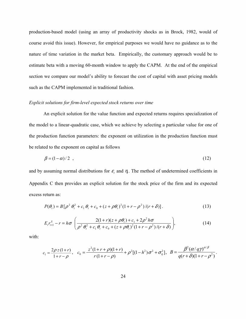
Explicit solutions for firm-level expected stock returns over time
An explicit solution for the value function and expected returns requires specialization of
the model to a linear-quadratic case, which we achieve by selecting a particular value for one of
the production function parameters: the exponent on utilization in the production function must
be related to the exponent on capital as follows
2/)1( αβ −= , (12)
and by assuming normal distributions for tε and tη . The method of undetermined coefficients in
Appendix C then provides an explicit solution for the stock price of the firm and its expected
excess return as:
)]/()1()([)( 2201
22 δρρθθθρθ +−+++++= rrzccBP tttt . (13)
+−+++++
++++=−+ )/()1()(
2))(1(222
0122
21
1 δρρθθθρσρρθσ
rrzcc
hczrhrrE
ttt
tStt , (14)
with:
ρ
ρ−++=
r
rzc
1
)1(21
, ])1[()1(
)1)(1( 22222
0 ησσρρ
ρ +−+−+
+++= hrr
rrzc ,
)1)((
)/(2
/2
ρδγαβ βα
−++=
rrq
qB .

25
Interpretation and discussion
For further intuition about the closed-form expression in equation (14), we consider a few
simple cases. As many of the comparative statics results are ambiguous (by nature in a
reasonably rich model) specific empirical implications are obtained in the next section for
standard parameter values.
Some of the comparative statics results are clear cut. Note first that the constant B does
not show up in the expected return expression as it multiplies both the price and the expected net
payoff. As a result, the production parameters, γα , do not affect the excess returns:
0/)( 1 =−+ αdrrEd Stt and 0/)( 1 =−+ γdrrEd S
tt . While these parameters do not affect the riskiness
of the operations, they affect profitability and thus are important for valuation, affecting the stock
price proportionately through B, but they affect the net payoff similarly so that the effect on
expected return vanishes.
The directional effect of depreciation is clear as well: 0/)( 1 >−+ δdrrEd Stt . An increased
depreciation rate raises the user cost of capital, here δ+r , thus lowering the optimal capital
stock, future profitability, and the price per share of the firm. The sensitivity to the factor risk
increases as a result of the diminishing returns to investment: at a decreased capital stock, the
marginal value of capital is larger so that given productivity shocks have a larger impact.
Higher variance of idiosyncratic productivity shocks 2ησ raises 0c and therefore increases
the stock price and decreases expected returns. This is consistent with the empirical results of
Ang, Hodrick, Xing, and Zhang (2006) which pose the puzzle that firms with higher
idiosyncratic risk have lower average returns. In our model higher idiosyncratic variability

26
enhances the option value arising from a firm’s flexibility to ramp production up or down with
changes in productivity: a positive shock is amplified by adding capital, and a negative shock is
mitigated by shedding capital. As evident from (A13) and (A14) and the definition of c0 in
Appendix C, higher idiosyncratic risk raises stock prices for given systematic operational risk.
Firms with higher idiosyncratic risk have lower average stock returns because the higher prices
for the given systematic risk imply less systematic operational risk per dollar invested.
For other parameters, the comparative statics are generally ambiguous. Typically, h (the
risk premium for the aggregate productivity shock) and σ (the sensitivity of firm productivity to
the aggregate productivity shock) increase the expected excess return. In addition, h usually
raises the firm’s beta (risk sensitivity). The reason is that an increase in h raises the cost of
capital which reduces the optimal capital stock, raises marginal productivity, and thus the
sensitivity to productivity shocks. An increase in the persistence of the shock, ρ , typically has a
positive effect on the expected excess return because it raises the strength of the firm’s reaction
to initial shocks (raising beta). Increases in both the long-run productivity level θ and the
current productivity level tθ raise the optimal capital stock, and therefore lower the marginal
productivity of capital. The latter reduces the marginal impact of productivity shocks and,
hence, risk sensitivity and expected stock returns.
Numerical solution for standard parameter values
We present some simple numerical results to obtain an idea of the quantitative
importance of particular responses, and generate comparative statics results for the empirically

27
relevant parameter space. We set h to 0.32. Since the Sharpe ratio is the volatility of the
stochastic discount factor divided by the expected value of the stochastic discount factor, from
equation (5) for the stochastic discount factor, h essentially defines the maximum Sharpe ratio of
an asset in this economy. The Sharpe ratio of the market return in our sample is 0.32. We set the
risk-free rate to 2.04% and the relative price of investment q equal to one.
As an imperfect proxy for the persistence of exogenous profitability factors, we set the
persistence of the level of productivity ρ to 0.89, the median of the AR1 coefficients of total
factor productivity of all industries in our sample. It is less persistent than the number reported in
King and Rebelo (1999), which is for aggregate productivity. The standard deviation of the
productivity shock is set to 0.37 and is similar to that used in Pastor and Veronesi (2003) and
Zhang (2005). Pastor and Veronesi (2003) show that the average volatility of firm-level
profitability has risen from 10% per year in the early 1960s to about 45% in the late 1990s.
Zhang (2005) sets the standard deviation of his firm-level productivity to 10% a month which
translates to 35% per year. Therefore, 37% (0.37) seems reasonable given the range estimated in
this literature. We set the deprecation rate δ to 8% a year, as in King and Rebelo (1999), and γ to
4% a year, as in McGrattan and Schmitz (1999), to reflect the fact that expenses related to
utilization are about half of physical capital investment (based on the sample of Canadian firms
examined by McGrattan and Schmitz).
We are left with two free parameters, α and θ (not β since it is tied to α), to match the
utilization-capital ratio (EK), the investment-capital ratio (IK), and the excess returns (Rse) in the
economy. To this end, we choose them to be 0.13 and 1.5, respectively. We also set tθ to its long

28
run average of 1.5 and this exercise shows (see Table 1) that the implied utilization-capital ratio
is 81.6%, close to that reported in Cooper, Gerald and Wu (2005), and the investment-to-capital
ratio is 11.3%, indicating a 1% average monthly depreciation combining normal depreciation and
utilization-related depreciation, and a 6.1% annual equity premium which are close to the
averages in our sample. The average investment return is 9.7%.15 In Figure 1, we show how u, i,
profits, and excess returns vary when tθ deviates from θ . We keep other parameters at their
original values and we vary tθ between 0.5 and 2.5. We confirm that, when tθ rises, both u and i
rise, and excess stock returns and profitability fall.
4. The Data
Test data are based on the COMPUSTAT annual file and the Manufacturing Industry
Database jointly provided by the National Bureau of Economic Research and the Center of
Economic Studies (NBER-CES).16 The model’s investment-to-capital ratio i (IK) is calculated
using firm-level COMPUSTAT data and is defined as the change in property, plant and
equipment plus the change in inventory normalized by lagged total assets. The capacity
utilization rate in the model u (EK) is calculated using industry-level NBER-CES data and is
defined as real spending on electricity (nominal spending deflated by the price index for
15 The gross average investment return is therefore 16.7%. This is less than half of the gross profit margin of the median firm, which is equal to 35.7% in Panel A of Table 2. In this dimension the average investment return thus is not a good proxy for the gross profit margin, and is a bit closer to the return on assets (which is 4.9% for the median firm in our sample, so 12.9% on a gross basis).
16 http://www.nber.org/nberces/nbprod96.htm.

29
electricity) divided by the real capital stock. Our industry-level data provide annual industry-
level historical figures for 459 industries on the stock of physical capital, spending on electricity,
their price indexes, and total factor productivity for the years from 1958 thru 2009. We merge the
NBER-CES data with the COMPUSTAT data by SIC code and assume that firms within an
industry have the same utilization rate. Note that real electricity use is, in principle, a very good
proxy for the intensity with which a firm’s resources are used. Whereas construction of standard
capacity utilization data requires arbitrary choices of what is labeled “full” capacity, electricity
usage provides a continuous measure combining the time period during which, and the intensity
with which, the firm’s total production capacity is utilized. 17
Monthly firm-level cum-dividend returns are taken from the Center for Research on
Stock Prices (CRSP), and the three-month T-bill rate is subtracted to calculate excess returns. To
obtain portfolio-level characteristics, we first calculate annual firm-level characteristics and then
take the means of the characteristics of all stocks that belong to each portfolio as the portfolio-
level characteristic. We consider various characteristics studied in Fama and French (2008): size
(price per share times shares outstanding), the book-to-market ratio (the book value divided by
the market value), the gross profit margin (the gross profit scaled by total assets), and momentum
(the cumulative excess return over the past 12 months). All firm-level accounting data are
obtained from COMPUSTAT. Excess market returns, SMB, HML, and the risk-free rate are
17 Earlier literature, such as Burnside, Eichenbaum and Rebelo (1995, 1996) also employs electricity usage as a proxy for capital utilization and finds that the resulting productivity shock differs substantially from the typical Solow residual-based productivity shock.
30
taken from Kenneth French’s website.18 Our sample starts at 1963 and ends at 2009 (limited by
the availability of the NBER-CES data).
Table 2 provides descriptive statistics of key variables. We first calculate the means of
these variables for each firm and then report their cross-sectional summary statistics. The median
IK ratio across all firms is 7.31%, with 80% of the firms in the range from -0.22% to 20.25%,
and the median EK ratio across all firms is 2.78%, with 80% of the firms between 1.18% and
6.8%. After fitting an autoregressive model of order one to each industry’s IK, EK, BM, and GP
at the cross-section, we find that median AR-1 coefficients are 0.92, 0.74, 0.95, and 0.95,
respectively, suggesting that the levels of investment, utilization, book-to-market, and
profitability are quite persistent. Therefore, factor sensitivities derived from these firm
characteristics are time-varying but likely to be reasonably stable. For the 558 months of our
sample period, the average values of the Market excess return, SMB, HML, and Risk free rate
are, respectively, 4.2%, 2.5%, 4.1%, and 4.5%.
5. Empirical Results
We address in turn the following sets of model implications: (1) the impact on excess
stock returns of firm-level production flow decisions, (2) the predictability of stock returns from
firm-level stocks and flows, (3) the performance of the production-based model in comparison to
traditional asset pricing models.
18 http://mba.tuck.dartmouth.edu/pages/faculty/ken.french/.

31
Investment and capacity utilization decisions effect on stock returns
Table 3 provides an initial look, employing one-way sorting, at the hypotheses that the
flows of capital investment and capital services both have a negative impact on required returns.
At June of each year t, we allocate all firms to five portfolios using year t-1 IK or EK quintile
values (with firm-level data for IK and industry-level data for EK). Portfolio L includes firms
with IK or EK values below the 20 percentile cutoff, and portfolio H includes industries with IK
or EK values above the 80 percentile cutoff values. Monthly portfolio excess returns from July of
year t to June of year t+1 are computed as the equal-weighted averages for the excess returns of
all firms in the portfolio. For each portfolio we report the equal-weighted excess return and
characteristics including market capitalization, book-to-market ratio, gross profitability margin,
investment-to-capital ratio, electricity-to-capital ratio, and cumulative excess return in the past
12 months.
Panel A presents the results for the five portfolios sorted by IK and EK. Portfolio L, with
the lowest 20% IK ratios, has monthly average return of 1.52%, Portfolio H (the highest 20% of
IK ratios) has average return of 0.95%. The return spread, L-H, is significantly positive as
predicted at 0.58% per month. When adjusting for risk using the Fama-French three-factor model
(1996), the risk-adjusted return is a bit lower at 0.48% but still significant. The Gibbons, Ross
and Shanken (1989) joint test of the five risk-adjusted excess returns reveals that these are jointly
significant as is consistent with Xing (2008) and Hou, Chen and Zhang (2012). Panel D in Table
2 shows that the correlations of monthly returns of the low minus high IK portfolio with the
market excess return, size factor and value factor are -0.18, 0.05 and 0.32 respectively. Panel B
in Table 3 presents characteristics of each of the five IK portfolios and the difference of

32
characteristics across low IK and high IK portfolios. We find that firms with larger IK ratios tend
to be growth firms and have performed relatively poorly in the past 12 months. These findings
are in line with those in Hou, Chen and Zhang (2012) in suggesting that an investment-based
asset pricing model is consistent with various financial market anomalies.
The results of sorting by EK are as follows. Here Portfolio L (lowest 20% EK ratios) has
an average monthly return of 1.37%, and Portfolio H (the highest 20% EK ratios) has average
return of 1.13%. The return spread, L-H, is positive as expected at 0.23% but not significant. The
risk-adjusted return is slightly higher and significant at 0.29% per month, and the GRS test
rejects the hypothesis of zero joint risk-adjusted excess returns. Correlations between the return
difference of the low EK portfolio and high EK portfolio and the market excess return, the size
factor, and the value factor are 0.28, 0.47, and -0.46 respectively (Table 2, Panel D). As does the
high IK portfolio, the high EK portfolio tends to include firms that have performed relatively
poorly in the past 12 months. High EK portfolio further are significantly less profitable and have
larger book-to-market ratios than low EK portfolios.
Table 4 presents the results of five-by-five double sorting of the firms into 25 portfolios,
so that we can control for the impact of a second selection criterion. In Panel A, in June of each
year t, we sequentially form five IK and then five EK portfolios using year t-1 information. We
calculate portfolio excess return as the equal-weighted average of excess returns of all firms in
the portfolio. For each level of EK, the return difference between low-IK and high-IK portfolios
is positive, at 0.60%, 0.71%, 0.69%, 0.52%, and 0.34%, confirming the importance of IK for
returns in the predicted direction. For each level of IK the return difference between high-EK
and low-EK portfolios is also positive as predicted but smaller, at 0.48%, 0.07%, 0.13%, 0.21%,

33
and 0.21%. The smaller excess returns and lower level of significance relative to IK may be
linked to the fact that firm-level EK values are instrumented by their industry values (one of 434).
The corresponding risk-adjusted excess returns are also positive for all low-EK minus high-EK
groups, and all low-IK minus high-IK groups. The GRS statistic is 6.04 with p-value of 0.0000,
which indicates that the risk-adjusted excess returns jointly deviate from zero. Panel B displays
the results for the reverse sequential sort, sorting first by EK and then by IK. These results are
similar to those in Panel A.
Predicting stock returns from production decisions and value indicators
Table 5 presents Fama and MacBeth (1973) regression results of using year t-1 EK, IK,
and other firm-characteristic variables to predict monthly industry-level excess returns starting
from July of year t to June of year t+1. The results are consistent with our earlier sorting results.
In Panel A, EK has a negative coefficient of -0.014 but is insignificant, IK has a significantly
negative coefficient of -0.012. When book-to-market (BM) is added in the regression, the
coefficient on IK is similar but the EK coefficient now is -0.024 and is marginally significant.
The coefficient on book-to-market is 0.0034 and is significant at the 1% level. We further control
for size, and stock price momentum in the past 12 months, and find that momentum remains a
robust indicator of future excess returns, but that the explanatory power of EK, IK, and BM
remains intact, when these variables are included.19
19 We also include a financial leverage variable as suggested by Liu, Whited, and Zhang (2009). However, this variable is insignificant in our sample and has no notable impact on the results so we omit it here.

34
Panel B presents Fama and MacBeth (1973) results using the same variables, but now to
predict profitability (measured by Gross Profit Margin, GP). As expected, EK negatively and
significantly predicts future profitability. On the other hand, IK has a positive (and marginally
significant) impact which is counter to our predictions. However, when we add BM in the
regression, and also when we further add size and momentum, both EK and IK have significantly
negative coefficients as expected.
While the value effect is confirmed strongly in this context as predicted, our model also
suggests specific firm characteristics for which we expect the effect to be reversed. Table 6
presents the extreme portfolios from a four-way sorting designed to examine the book-to-market
effect for firms with returns on assets predicted to be below the appreciation rate on intangible
assets. This is uncommon, because of the submartingale property of risk-adjusted tangible assets
and the supermartingale property of risk-adjusted intangible assets, so we choose firms with the
highest EK and IK ratios as this predicts the lowest return on tangible assets (average investment
return); and firms with the highest growth of research and development expenses per unit of
capital (RDG) as a predictor of a high appreciation rate of intangible assets. While usage of
R&D as a sorting variable eliminates a large fraction of the data (only 20% of COMPUSTAT
firm-year observations have R&D measures), in this instance we attempt to identify the specific
and presumably small subset of firms anticipated to have change in intangible assets larger than
the tangible return and it seems essential to search for them within the set of firms with high
R&D: the high RDG firms are expected to have larger intangible returns while their tangible
returns measured as gross profits are not affected (which, as Novy-Marx, 2013, stresses, presents
an advantage of sorting by gross profits). To have a reasonable number of firms in each cell

35
(portfolio) we start the sample in 1981 which implies an average of around 150 firm years in
each cell.
In Panel A we first sort firms by RDG – the growth of each firm’s R&D expenses,
normalized by lagged total assets to reflect the overall importance of R&D for this firm. We put
the 30% firms with lowest RDG in portfolio L and the 30% firms with highest RDG in portfolio
H. The second sorting criterion addresses the investment returns, and we again put the firms with
30% highest IK and EK in portfolios H and those with the 30% lowest IK and EK in portfolios L.
The prediction is that the returns of higher RDG and IK/EK firms exhibit a smaller value effect,
and that the value effect is actually reversed for the highest RDG and IK/EK firms. Panel A
shows that, indeed, the value effect (return difference between highest 30%, H, and lowest 30%,
L, book-to-market ratio firms) reverses for firms, with the above 70-th percentile (marked by H)
in RDG, IK, and EK: portfolios 15 and 16. The effect is small, a little below one percent
annually, and not significant. However, the value effect has the standard positive sign in all other
cases, for which at least one of the sorting variables is below the 30-th percentile (marked by L),
and is, generally, the larger the more of the sorting variables are in bottom 30% , L, portfolios.
Performance of traditional and production-based approaches
Table 7 provides a forecast experiment in which the impact of EK, IK, and BM is
allowed to be time-varying. We predict excess returns based on the parameters of cross-sectional
regressions of firm-level excess returns on the forecast variables (EK and IK, with or without
BM). At June of year t, we form five portfolios from predicted excess returns, which are
calculated using information variables from December of year t-1 and average coefficients across

36
previous periods. We consider two sets of average coefficients: those that use data of the
previous 10 years, and those that use data up to date (Rolling, Expanding). Portfolio H has the
highest predicted returns (Pred). For each portfolio, we then track its excess return from July of
year t to June of year t+1 and report the average realization (Real). We follow a similar
approach for two competing models: the CAPM and the Fama-French three-factor model. Here
for the “rolling” case we estimate betas using five years of data (the standard 60 monthly data
points) and for the “expanding” case we use all previous data points to estimate betas.
The results indicate that each of the models generates a reasonable spread between
Portfolio H (20% firms with the highest predicted returns) and Portfolio L (20% firms with the
lowest predicted returns), ranging from 0.58% per month (IK and EK), 0.64% (CAPM), 0.80%
(Fama-French three-factors), to 0.95% (IK, EK, and BM). However, the prediction errors differ
dramatically between the models. The mean squared errors (MSE) computed from the
differences between predicted and realized returns for each of the five portfolios are far lower for
both the IK and EK, and the IK, EK, and BM models compared to the CAPM and Fama-French
model by at least a factor three. When we standardize the prediction errors by the total variation
in predicted returns, the difference is even more pronounced. We also present t-statistics for the
differences between the realized and predicted returns. The discrepancy between predicted and
realized difference for Portfolio H versus Portfolio L is statistically significant for the CAPM and
Fama-French models but not for our models. In fact, the CAPM and the Fama-French models
perform worse than the average random draw as returns from buying portfolio H and selling
portfolio L are negative! Table 8 shows that these results are quite consistent over the decades.

37
We thus provide strong empirical evidence for the simulation-based results of Lin and
Zhang (2013) that production-based models outperform traditional models: although the
production-based and traditional consumption-based approaches theoretically are two sides of
the same coin, the production-based approach seems to work better in predicting a firm’s cost of
capital.
6. Conclusion
In traditional estimation of required returns, factor sensitivities are obtained from time
series of returns and factor realizations. Empirically motivated conditioning approaches aside,
the tradition of estimating factor sensitivities from simple time series persists in spite of the
theoretical contributions of Cox, Ingersoll, and Ross (1985) and Berk, Green, and Naik (1999)
that provide a framework for firm choice of risk sensitivities. Given the prices of risk as
determined economy-wide and the market and productivity conditions at the firm level,
individual firms choose their production and investment activities to supply risk – firms choose
their sensitivities to risk factors. The resulting sensitivities depend on firm-level characteristics
implied by the market and productivity constraints faced by the firm, and can be estimated
structurally.
The investment-based approach of Cochrane (1991, 1996) provides a specific market and
productivity environment for firm choices that has been limited to constant returns to scale
technologies. But the limitation is mostly for the sake of tractability and we avoid it here with the
purpose of focusing on endogenous fluctuations in profitability. We find that higher investment
and production (capacity utilization) choices both are associated with a lower marginal product

38
of capital which decreases the sensitivity of a firm to the risk of productivity shocks. As a result,
risk sensitivities and required stock returns decrease as do investment returns and standard
profitability measures.
At the same time, book-to-market ratios have a measurable impact on required returns
that is separate from profitability. For given expected profitability of book assets (the tangible
capital stock) higher book-to-market ratios imply more risk sensitivity: given mean reversion,
current shocks to capital productivity have more impact when a larger fraction of shareholder
equity is tied up in tangible assets. An exception is for uncommon cases in which expected
returns on tangible capital are smaller than expected appreciation rates of intangible assets. In
these cases we expect an inverted value effect because higher book-to-market ratios now imply
less overall risk as the importance of intangible assets is reduced relative to tangible assets and,
quantitatively in these uncommon cases, the effect of lower exposure to the risk of reduction of
intangible asset values dominates the effect of higher exposure to the risk of tangible assets.
The theoretical results support the finding by Novy-Marx (2013) of dual dimensions to
value – profitability levels and book-to-market levels – both raising required returns. Our view is
that higher profitability relates to higher average product of capital making firms more sensitive
to current productivity shocks. A higher book-to-market ratio further increases the sensitivity to
productivity shocks as this implies less weight on the intangible asset component which has
relatively low loadings on the current productivity shocks. Empirically, we confirm that both the
level of capital expansion and the level of capital utilization predict lower required returns, and
that higher book-to-market value is associated with higher required returns, the traditional value

39
effect. But we also provide an indication that the value effect is inverted in the predicted cases –
for firms with low expected profitability and high expected intangible asset appreciation.
Our results hinge on an intangible asset perspective that parts ways with that of the
growth options literature (Berk et al., 1999) and the investment-based asset pricing literature
(Cochrane, 1996). The view of this literature is that book-to-market ratios deviate from one
because the ability of firms to profitably expand their future activities is not incorporated in book
values yet is priced in the market. But, in our model, firms can expand to their desired size
without friction so intangible asset values are not related to expansion options. They arise as the
present value of future residual income stemming from decreasing returns to scale and/or market
power (and may also be tied to the earnings power of capitalized previous research and
development expenses, although we do not model this aspect). These intangible asset
components have in common that they add to profitability, but because of the documented mean
reversion of profitability (Fama and French, 2000 and 2006), are less sensitive than tangible
assets to current productivity shocks.
Discarding the constant returns to scale formulation in the investment-based framework
is vital for generating the positive co-movement between a firm’s expected stock returns and
profitability in our model. Firms with stronger decreasing returns have higher profit margins
resulting from increased leverage of the marginal investment return, but the leverage of the
marginal investment return also implies proportionately higher risk, and therefore higher
expected stock returns. In contrast, the literature starting with Carlson et al. (2004) relies on
operating leverage to generate fluctuations in risk and return. Operating leverage and risk
increase with the fixed costs of capital in place, but profitability decreases with this fixed cost,

40
generating a counterfactual negative co-movement between expected return and profitability as
stressed by Kogan and Papanikolaou (2013) and Novy-Marx (2013).
We further offer a direct comparison between the performance of the traditional asset
pricing approach and the production-based asset pricing approach to predict required returns or
costs of capital. Lin and Zhang (2013) provide simulation results supporting the production-
based perspective; we provide empirical results in support of this approach. In comparison with
the CAPM and the Fama-French three-factor model, with factor sensitivities estimated from time
series, we find that our production-based model, with structural estimation of factor sensitivities,
performs better in two dimensions: (1) generating more variation in predicted returns across
assets, and, especially, (2) predicting realized asset returns.
Production-based asset pricing provides a promising complement to traditional asset
pricing. It affords new insights into the supply of risk which may prove to provide better clues
about variation in the cost of capital and methods for determining more reliable estimates of this
important financial decision gauge. Our theoretical and empirical results suggest that a more
detailed view of production decisions is already useful in generating better forecasts of the cost
of capital, and also points at additional production-based variables that may provide a direction
for further improvements to cost of capital estimation in future production-based asset pricing
research.

41
Appendix
A. The optimal capital stock and investment returns The solution for optimal investment from equation (6) requires further information about the
value function. We obtain a “concentrated” current value function by substituting equations (3) and (2)
into the Bellman equation (1) and then using equation (8) to eliminate tU . Then
)],([)1()/)(1(),( *111
*1
11++++ +−−+−= −−
tttttttttt KVmEqKqKKqKV θδθγααθ αβ
αα
, (A1)
where *1+tK is the capital stock implied by the optimal investment policy. The marginal value of capital,
),( 11 ++ ttK KV θ may be obtained straightforwardly by updating the concentrated value function by one
period and using the envelope theorem:
qKqKV ttttK )1()/(),(1
111111 δθγαβθ α
βα
α
−+= −++++
−− . (A2)
Thus, )()/(/)]()1(1[ 111
1
111
+++−
+−− −−= tttttt mEqqmEK θγαβδ αα
αβ
from equations (6) and (A1). The functional
forms in equations (4) and (5) imply straightforwardly that
)1/()()( 11 rzmE tttt ++=++ ρθθ , σθρ hz −−≡ )1( . (A3)
Equation (9) follows:
βαα
ρθ −−−
+=+1
1
)]([*1 tt zAK , )(/)/( 1 δγαβ α
α
+≡ − rqqA . (A4)
From (A2), (A3), and (A4), using the definition qKVr ttKI
t /),(1 111 +++ ≡+ θ we obtain equation (10):
)()( 11
1 δθρ
ηεσ +
+
++=− +++ r
z
hrr
t
ttIt
. (A5)
B. Components of stock returns
From (A4) it is clear that *1+tK is a function of
tθ and nottK . Hence, we may express the
disembodied component of equity value, the intangible assets, as:
)],([,)( *111
*1 ++++ =−= tttttttt KVmEPqKPG θθ . (A6)
We derive explicitly the relation between investment returns and stock returns. From (A1), (A2), and (A6), and using the definition ββα /)1( −−=s :
[ ] )()1(),()1(),( 111111 ++++++ +−−+= tttKttt GqsKVsKKV θδθθ . (A7)
To obtain equation (11), the expression for stock returns, divide by the stock price on both sides and then
subtract one on both sides (net returns are in lower case: 1−≡ Xt
Xt Rr ):
)](1)[,()( 111 tttttS
t bgbr θθθθπ −+= +++ , )( δπ ++≡ It
Itt rsr . (A8)
Here ttt PKqb /)( 1+=θ is the book-to-market ratio and )(/)]()([),( 11 ttttt GGGg θθθθθ −= ++ is the rate of
increase in the firm’s intangible assets.

42
We define )( δπ ++= It
Itt rsr representing the average return on investment which equals the
marginal return on investment Itr (given in A5) plus a markup due to decreasing returns to scale. Gross
average return also equals: )1(]/),([))(1( δθδδπ −−=++=+ qKVrs ttkI
tt . From (A2) we have
qKqqKV ttttK /)/()1(]/),([ 111 −−−=−− αβ
αα
θγαβδθ . Then from βααθ tttt KUY −= 1 and equation (8) we
obtain qKqqKUY ttttt /)/)(1(/)(1
11−−−−=− α
βα
α
θγααγ . It follows that the gross average return on
investment also equals the gross profit margin, tttt qKUY /)( γδπ −=+ .
To prove that the book-to-market ratio is always less than one in our model with decreasing
returns to scale, we need to show that 0)( *1 >−= +ttt qKPG θ (which implies 1/*
1 <+ tt PqK ). Multiply
(A7) by 1+tm and take expectations. This yields from ββα /)1( −−=s and equation (6) that
)]([)]1/()(1[)],([ 111111 ++++++ ++++= tttttttt GmEqKrrsKVmE θδθ . From (A4) and (A6) then
)]([1
)()( 111 +++ +
++= ttttt GmEKqr
rsG θδθ . (A9)
Equation (A9) entails by induction that, for all t, 0)( >tG θ since 01 >+tK and 0>s .
Intangible asset values adjusted for risk and time value follow a strict supermartingale process:
since tttt GGmE <++ )( 11 for 0>s from (A9), we have 1)]1([ 11 <+ ++ ttt gmE . Similarly, tangible asset values
adjusted for risk and time value follow a strict submartingale process: because investment returns are a
martingale 1)]1([ 11 =+ ++I
ttt rmE it follows from )( 111 δπ ++= +++I
tI
tt rsr that 1)]1([ 11 >+ ++ ttt mE π for
0>s .
Since tttt GGmE <++ )( 11 , the adjusted value of intangible assets must decrease over time. However,
the expected growth rate of intangible assets, tttttt GGGEgE /])([)( 11 −= ++ , may be expected to either be
positive or negative depending on whether the interest cost and the systematic risk compensation together exceed or fall short of the “supermartingale deficit”, 1)]1/()([ +++ tKqrrs δ . Note, however, that the
unconditional average growth rate of intangible assets must be zero due to the stationarity of the
productivity shock process: 0)( 1 =+tgE .
From 1)]1([ 11 =+ ++I
ttt rmE it follows that It
Itt RPrrE +=+ )( 1 (with IRP the risk premium for the
investment return). So It
It
It
Ittt CRPRPrsRPrE +=+++=−+ )()( 1 δπ , with 0>I
tC . Further,
1))],(1([ 11 <+ ++ tttt gmE θθ so that Gt
Gtttt CRPrgE −+=+ ),( 1 θθ , with 0>G
tC from the strict
supermartingale nature of the intangible assets. Hence, the effect on the expected excess stock return
rrE Stt −+ )( 1 of an increase in the book-to-market ratio tb , taking expectations in equation (15), equals
Gt
It
Gt
Ittttt RPRPCCgE −++=− ++ )],([ 11 θθπ which is typically positive unless the risk premium on
intangible assets, GtRP , and thus ),( 1 ttt gE θθ + , is unusually large.

43
C. Explicit solutions for firm-level expected stock returns over time Assume normality and set 2/)1( αβ −= , (A10)
Proceed by employing the method of undetermined coefficients given a quadratic assumption for )( tG θin equation (A9). It is straightforward, but tedious, from equations (A9), (4), and (5) to confirm the quadratic solution for the following specific parameter values:
)()( 012
2 cccBG ttt ++= θθθ , (A11)
with 22 ρ=c ,
ρρ
−++=
r
rzc
1
)1(21 , ])1[(
)1(
)1)(1( 22222
0 ησσρρ
ρ +−+−+
+++= hrr
rrzc , and
)1)((/)/( 2/2 ρδγαβ βα −++≡ rrqqB .
(A1) becomes from equations (A10) and (A11):
012
2½ )1()/)(1(),( 1 cccqKKqKV ttttttt +++−+−= − θθδθγααθ α
α
, (A12)
From equations (A4) and (A6) we can also find the stock prices as
)]/()1()([)( 2201
22 δρρθθθθ +−+++++= rrzcccBP tttt . (A13)
The expected return is ttttS
tt PKVEhrrE /)],([ *111 +++ =− θσ θ : From )]1([1 11
ittt rmE ++ += and the
definition of (conditional) covariance, the expected net stock return of the firm is
),/( 1111S
tttttS
tt rmEmCovrrE ++++ −= . Using the definition of return and the stochastic discount factor
specification in equation (5) thenttttt
Stt PKVEhrrE /)],([ *
1111 ++++ =− θε .Given the normality of 1+tε ,
Stein’s Lemma implies that )],([)/( *111 +++ =− tttt
Stt KVEPhrrE θσ θ . Straightforward subsequent derivation
provides the closed-form solution for the expected excess stock return as
+−+++++
++++=−+ )/()1()(
2))(1(222
0122
21
1 δρρθθθρσρρθσ
rrzcc
hczrhrrE
ttt
tStt
. (A14)

44
References
Abel, A. B., and J. C. Eberly, 2011. How Q and Cash Flow Affect Investment without Frictions: An Analytic Explanation. Review of Economic Studies 78, 1179-1200.
Ang, A., R. J. Hodrick, Y. Xing, and X. Zhang, 2006. The Cross-Section of Volatility and Expected Returns. Journal of Finance 61, 259–299.
Balvers, R. J., T. Cosimano and B. McDonald, 1990. Predicting Stock Returns in an Efficient Market. Journal of Finance, 1109–1128.
Balvers, R. J., and D. Huang, 2007. Productivity-Based Asset Pricing: Theory and Evidence, Journal of Financial Economics 86, 405–445.
Belo, F., S. Bazdresch, and X. Lin, 2013. Labor Hiring, Investment and Stock Return Predictability in the Cross Section, Forthcoming Journal of Political Economics.
Berk, J. B., R. C. Green, and V. Naik, 1999. Optimal Investment, Growth Options, and Security Returns. Journal of Finance 54, 1553–1607.
Bloom, N., 2009, The Impact of Uncertainty Shocks, Econometrica 77, 623–685.
Boldrin, M., L. J. Christiano, and J. D. Fisher, 2001. Habit Persistence, Asset Returns, and the Business Cycle, American Economic Review 91, 149-166. Booth, L., B. Chang, W. Hejazi, and P. Shum, 2008. The Influence of Productivity on Asset Pricing, Working Paper University of Toronto.
Brock, W. A., 1982. Asset Prices in an Exchange Economy. in John J. McCall, ed.: The Economics of Information and Uncertainty, University of Chicago Press, Chicago.
Burnside, C., M. Eichenbaum, and S. Rebelo, 1995. Capital Utilization and Returns to Scale. NBER Macroeconomics Annual.
Burnside, C., M. Eichenbaum, and S. Rebelo, 1996. Sectoral Solow Residuals. European Economic Review 40, 861–869.
Caballero, R. J., 1999. Aggregate Investment, in John B. Taylor and Michael Woodford, eds., Handbook of Macroeconomics (New York: Elsevier), 816–862.
Carlson, M., A. Fisher, and R. Giammarino, 2004. Corporate Investment and Asset Pricing Dynamics: Implications for the Cross-Section of Returns. Journal of Finance 59, 2577–2603.

45
Chen, L., and L. Zhang, 2011, Do Time-Varying Risk Premiums Explain Labor Market Performance?. Journal of Financial Economics 99, 385–399.
Cochrane, J. H., 1991. Production-Based Asset Pricing and the Link Between Stock Returns and Economic Fluctuations, Journal of Finance 46, 209–237.
Cochrane, J. H., 1996. A Cross-Sectional Test of an Investment-Based Asset Pricing Model. Journal of Political Economy, 104, 572–621.
Cooper I., 2006. Asset Pricing Implications of Nonconvex Adjustment Costs and Irreversibility of Investment. Journal of Finance 61, 139–170.
Cooper I., B. Gerald, and G. Wu, 2005. Investment Irreversibility, Real Activity and the Value Premium. Working paper.
Cox, J.C., Ingersoll Jr, J.E., Ross, S.A., 1985. An Intertemporal General Equilibrium Model of Asset Prices. Econometrica 53, 363–384.
Da, Z. and H. Yun. 2010. Electricity Consumption and Asset Prices. Working paper, University of Notre Dame.
Fama, E. F., and K. R. French. 1995. Size and Book-to-Market Factors in Earnings and Returns. Journal of Finance 50, 131-155
Fama, E. F., and K. R. French. 1996. Multifactor Explanations of Asset Pricing Anomalies. Journal of Finance 11, 55–84.
Fama, E. F., and K. R. French. 2000. Forecasting Profitability and Earnings. Journal of Business 73, 161-175.
Fama, E. F., and K. R. French. 2006. Profitability, Investment, and Average Returns. Journal of Financial Economics 82, 491-518.
Fama, E. F., and K. R. French. 2008. Dissecting Anomalies. Journal of Finance 63, 1653–1678.
Fama, E.F., and J. MacBeth. 1973. Risk, Return, and Equilibrium: Empirical Tests, Journal of Political Economy 91, 607–636.
Gibbons, M. R., S. A. Ross, and J. Shanken. 1989. A Test of the Efficiency of a Given Portfolio. Econometrica, 57, 1121–1152.
Gomes, J. F., L. Kogan, and L. Zhang, 2003. Equilibrium Cross-Section of Returns, Journal of Political Economy 111, 693–732.

46
Hall, R. E., 2004. Measuring Factor Adjustment Costs, Quarterly Journal of Economics 119, 899–927.
Hayashi, F., 1982. Tobin's Marginal q and Average q: A Neoclassical Interpretation, Econometrica 50, 213–224.
Hou, K., Xue, C., Zhang, L., 2012. Digesting Anomalies: An Investment Approach. Working Paper. The Ohio State University.
Hsu, P., 2006. Aggregate Technology Shocks and Market Return Predictability. Working Paper. Graduate School of Business, Columbia University.
King, R., S. T. Rebelo, 1999. Resuscitating Real Business Cycles. John B. Taylor and Michael Woodford, eds., Handbook of Macroeconomics, Elsevier Science Publications, Chapter 14: 927–1007.
Li, D., and L. Zhang, 2010. Does q-Theory with Investment Frictions Explain Anomalies in the Cross-Section of Returns? Journal of Financial Economics 98, 297–314.
Li, E., D. Livdan, and L. Zhang, 2009. Anomalies. Review of Financial Studies 22, 4301– 4334.
Lin, X., and L. Zhang, 2013. The Investment Manifesto. Journal of Monetary Economics 60, 351–366.
Lioui, A., and P. Poncet, 2008. Production-Based Asset Pricing in a Monetary Economy: Theory and Evidence. Working Paper EDHEC Risk and Asset Management Research Centre.
Liu, L.X., T. M. Whited, L. Zhang, 2009. Investment-Based Expected Stock Returns. Journal of Political Economy 117, 1105–1139.
McGrattan E.R., and J. Schmitz, 1999. Maintenance and Repair: Too Big to Ignore. Federal Reserve Bank of Minneapolis Quarterly Review 23, 2–13.
Newey, W. K., and K. D. West, 1987. A Simple, Positive Semi-Definite, Heteroskedasticity and Autocorrelation Consistent Covariance Matrix, Econometrica 55, 703–708.
Novy-Marx, R., 2011. Operating leverage. Review of Finance, 15, 103–134.
Novy-Marx, R., 2013. The Other Side of Value: The Gross Profitability Premium, Journal of Financial Economics 108, 1–28.
Pastor, L., and P. Veronesi, 2003, Stock Valuation and Learning about Profitability. Journal of Finance 58, 1749–1789.

47
Restoy, F. and G. M. Rockinger. 1994. On Stock Market Returns and Returns on Investment, Journal of Finance, 543–556.
Titman, S., K. C. Wei, and F. Xie, 2004. Capital Investments and Stock Returns, Journal of Financial and Quantitative Analysis 39, 677–700.
Tobin, J., 1969, A General Equilibrium Approach to Monetary Theory, Journal of Money Credit and Banking 1, 15–29.
Xing, Y., 2008, Interpreting the Value Effect Through the Q-theory: An Empirical Investigation, Review of Financial Studies 21, 1767–795.
Zhang, L., 2005, “The Value Premium,” Journal of Finance 60, 67–103.

48
Table 1. Numerical Solution for Typical Parameter Values
We set the physical capital depreciation rate, δ, to 0.08 as in King and Rebelo (1999), γ to 0.04 to account for McGrattan and Schmitz’s (1999) finding that maintenance expenses related to utilization are approximately half of that of physical capital investment, the persistence of the productivity, ρ, to 0.89, which is the median of AR-1 coefficients of total factor productivity (using all industries in our sample), the standard deviation of the productivity shock, σ to 0.37, as in Zhang (2005), the risk-free rate, r, to 0.0204, h, to 0.32, which is the Sharpe ratio of the market excess return in our sample. We then set α to 0.131 and⎯θ and θt to 1.5 to achieve reasonable estimates for the investment rate (IK), the utilization rate (EK), the average investment return (Rgp), and the equity premium (Rs
e).
α β δ γ
0.1310 0.4345 0.0800 0.0400
ρ ⎯θ σ
0.8900 1.5000 0.3700
r b q
0.0204 0.3200 1.0000
u i Rse Rgp
0.8182 0.1127 0.0610 0.0972

49
Table 2. Summary Statistics, 1963/07-2009/12
In Panel A, we present the mean, median, 10th percentile and 90th percentile values, and standard deviation (Mean, Median, P10, P90, Std) of the Investment-to-Capital ratio, the Electricity-to-Capital ratio, the Book-to-Market ratio, and the Gross Profit Margin (IK, EK, BM, and GP) across all firms. EK is calculated using the NBER-CES Manufacturing Industry Database obtained from http://www.nber.org/nberces/nbprod96.htm. It is defined as real spending on electricity (spending deflated by the price index for electricity) divided by the real capital stock. IK is the Investment-to-Capital Ratio, which is defined as the sum of changes in gross property, plant and equipment (COMPUSTAT item PPEGT) and change in inventory (INVT) scaled by lagged total assets (AT). GP is gross profit margin and it is the gross profit margin (COMPUSTAT item GP) normalized by total assets. In Panel B we report the AR1 time series correlations across all firms for IK, EK, BM, and GP. Panel C reports means and t-values of time-series of the excess market return, SMB, and HML, as well as two Low minus High portfolios constructed from IK and EK (IK L-H, EK L-H). Panel D reports the correlations of these variables. To construct the Low minus High IK/EK portfolios, we merge industry-level EK to CRSP-COMPUSTAT firms by 4-digit SIC code. At June of each year t, we allocate all firms into five quintiles based on the IK or EK values available at the end of year t-1, and we track monthly excess returns of these firms from July of year t to June of year t+1. Portfolio excess returns are the equal-weighted averages of excess returns of firms in each portfolio. Portfolio 1 (L) includes firms with IK or EK values below the 20th percentile, and Portfolio 5 (H) includes firms with IK or EK values above the 80th percentile, etc. IK L-H or EK L-H is the difference in returns of Portfolio L and Portfolio H. Excess market return, SMB and HML returns are taken from http://mba.tuck.dartmouth.edu/pages/faculty/ken.french/ (Kenneth French’s website).
Panel A: Average EK across Firms
Variable Mean Median P10 P90 Std
IK 0.1012 0.0731 -0.0022 0.2025 0.2647 EK 0.0359 0.0278 0.0118 0.0680 0.0328 BM 0.9727 0.7590 0.2256 1.8982 0.9874 GP 0.3556 0.3571 0.1083 0.6545 0.2901
Panel B: Average AR1 Correlation across Firms
Variable Mean Median P10 P90 Std
IK 0.9104 0.9186 0.8711 0.9532 0.0584 EK 0.4949 0.7366 -0.3895 0.9737 0.5700 BM 0.9309 0.9455 0.8740 0.9803 0.0655 GP 0.9343 0.9501 0.8740 0.9832 0.0643
Panel C: Factors
IK LMH EK LMH MKT SMB HML
Mean 0.0058 0.0023 0.0042 0.0025 0.0041 t-value 6.5198 1.5954 2.2118 1.8704 3.2873
Panel D: Correlations
Corr. IK L-H EK L-H MKT SMB HML
IK L-H 1.0000 0.0577 -0.1800 0.0543 0.3151 EK L-H 1.0000 0.2801 0.4651 -0.4586
MKT 1.0000 0.3045 -0.3220 SMB 1.0000 -0.2404 HML 1.0000

50
Table 3. Portfolios Formed on IK or EK, One-dimensional Sorting, 1963/07-2009/12
At June of each year t, we allocate all firms to five quintile portfolios based on cutoff values for the IK or EK variables available at the end of year t-1, and we track monthly excess returns of these firms from July of year t to June of year t+1. Portfolio excess returns are equal-weighted averages of excess returns of firms in each portfolio. Portfolio L includes firms with IK or EK values below the 20th percentile, and Portfolio H includes firms with IK or EK values above the 80th percentile, etc. Industry-level EK values are computed using data from the NBER-CES Manufacturing Industry Database. For each portfolio, in Panel A we report the mean of the portfolio excess return (Ret), and risk-adjusted returns (Alpha) from the Fama-French (1996) three-factor model. In Panel B we report average portfolio characteristics, which include market capitalization, book-to-market ratio, gross profit margin, investment-to-capital ratio, electricity-to-capital ratio, and cumulative excess return in the past 12 months (ME, BM, GP, IK, EK, MOM). The GRS statistic and its p-value in Panel A are the results from a joint test of the significance of risk-adjusted returns of the quintile portfolios following Gibbons, Ross and Shanken (1989).
Panel A: Returns and Alphas
Variables Ret. L 2 3 4 H L-H
IK mean 0.0152 0.0138 0.0131 0.0120 0.0095 0.0058 t-value 5.5856 5.7723 5.7356 5.0267 3.4933 6.5198 Alpha 0.0063 0.0059 0.0056 0.0047 0.0015 0.0048
t-value 5.8430 7.6967 7.7920 6.4230 1.7117 5.7085 GRS 25.0540 p-value 0.0000
EK mean 0.0137 0.0137 0.0130 0.0119 0.0113 0.0023 t-value 4.7346 5.4476 5.3875 4.7032 4.8623 1.5954 Alpha 0.0062 0.0059 0.0052 0.0035 0.0033 0.0029
t-value 5.5467 6.0558 6.4862 3.8681 3.8969 2.3554 GRS 11.6052 p-value 0.0000
Panel B: Characteristics
IK Char. L 2 3 4 H IK L-H
ME 1195.6 2359.5 2474.9 2355.6 1332.0 -136.4 BM 1.2360 1.0528 0.9444 0.8330 0.7683 0.4677 GP 0.3648 0.3813 0.4073 0.4269 0.3990 -0.0342 IK -0.0781 0.0248 0.0627 0.1098 0.3162 -0.3942
EK 0.0387 0.0393 0.0417 0.0422 0.0425 -0.0038 MOM 0.1195 0.0903 0.0836 0.0685 0.0406 0.0790
EK Char. L 2 3 4 H EK L-H ME 2170.9 2173.9 1771.4 1434.8 2133.7 37.2
BM 0.8834 0.8555 0.9420 1.0220 1.1339 -0.2504 GP 0.4310 0.4178 0.4085 0.4068 0.3167 0.1143 IK 0.0789 0.0882 0.0859 0.0876 0.0948 -0.0160
EK 0.0158 0.0236 0.0301 0.0418 0.0933 -0.0776 MOM 0.0879 0.0913 0.0823 0.0752 0.0658 0.0221

51
Table 4. Portfolios Formed on IK and EK, Two-dimensional Sorting, 1963/07-2009/12
We sequentially form 25 portfolios based on the IK and EK values. In Panel A, each June we first form five IK portfolios and then divide each IK portfolio into five EK portfolios using all firms. The portfolio excess return is the equal-weighted average of firm excess returns from July of year t to June of year t+1. Portfolio 1 (L) has the lowest 20% IK or EK values and portfolio 5 (H) has the largest IK or EK values. For each portfolio, we record its mean excess returns and risk-adjusted returns (Alpha) using the Fama-French three-factor model (1996). The GRS statistic is a joint test of whether risk-adjusted returns significantly deviate from zero, following Gibbons, Ross and Shanken (1989). Panel B reverses the sorting order, sorting by EK first and IK second.
Panel A: Sequential Sorting on IK and EK
Ret. IK-L IK-2 IK-3 IK-4 IK-H IK L-H Alpha IK-L IK-2 IK-3 IK-4 IK-H IK L-H
EK-L 0.0170 0.0136 0.0130 0.0129 0.0110 0.0060 0.0095 0.0057 0.0061 0.0057 0.0038 0.0057
EK-2 0.0166 0.0155 0.0142 0.0124 0.0095 0.0071 0.0072 0.0080 0.0068 0.0055 0.0018 0.0055
EK-3 0.0162 0.0137 0.0140 0.0118 0.0093 0.0069 0.0075 0.0060 0.0064 0.0045 0.0014 0.0061
EK-4 0.0139 0.0132 0.0121 0.0120 0.0087 0.0052 0.0040 0.0052 0.0045 0.0044 0.0001 0.0039
EK-H 0.0123 0.0129 0.0118 0.0108 0.0089 0.0034 0.0035 0.0046 0.0039 0.0033 0.0007 0.0028
EK L-H 0.0048 0.0007 0.0013 0.0021 0.0021 0.0081 0.0061 0.0011 0.0022 0.0024 0.0031 0.0064
t-value
EK-L 5.2114 4.7955 5.0065 4.4639 3.1930 3.4261 5.3931 4.3512 5.2881 4.4759 2.1959 3.2597
EK-2 5.5367 6.1186 5.9382 4.9293 3.3477 4.2706 4.4631 6.8027 6.2541 4.9775 1.3808 3.3207
EK-3 5.8236 5.4227 5.7862 4.7460 3.3763 4.4120 5.2682 4.7528 5.5624 3.9328 1.1344 3.8632
EK-4 4.7254 5.2433 5.2711 4.8918 2.9869 3.4408 2.9790 4.4504 4.7047 4.1866 0.0865 2.6192
EK-H 4.6568 5.4282 4.9226 4.6347 3.4139 2.3446 2.5788 4.4504 3.5214 3.1528 0.5593 1.9154
EK L-H 2.2586 0.4024 0.8333 1.2200 0.9449 3.7100 3.1334 0.7050 1.4868 1.5348 1.5379 4.3300
GRS 6.0392
p-value 0.0000
Panel B: Sequential Sorting on EK and IK
Ret. EK-L EK-2 EK-3 EK-4 EK-H EK L-H Alpha EK-L EK-2 EK-3 EK-4 EK-H EK L-H
IK-L 0.0176 0.0170 0.0155 0.0133 0.0133 0.0043 0.0092 0.0082 0.0067 0.0034 0.0044 0.0048
IK-2 0.0138 0.0149 0.0129 0.0131 0.0124 0.0015 0.0064 0.0072 0.0051 0.0049 0.0044 0.0020
IK-3 0.0130 0.0145 0.0140 0.0137 0.0119 0.0011 0.0059 0.0070 0.0065 0.0058 0.0040 0.0019
IK-4 0.0122 0.0125 0.0112 0.0109 0.0102 0.0020 0.0048 0.0057 0.0043 0.0032 0.0030 0.0018
IK-H 0.0108 0.0102 0.0107 0.0090 0.0088 0.0019 0.0036 0.0025 0.0027 0.0005 0.0007 0.0029
IK L-H 0.0068 0.0069 0.0048 0.0043 0.0045 0.0088 0.0056 0.0057 0.0040 0.0030 0.0055 0.0055
t-value
IK-L 5.3789 5.7978 5.6378 4.5288 5.0258 2.1111 5.3001 4.9562 5.1246 2.4280 3.2680 2.5406
IK-2 4.9127 5.7788 5.2242 5.2735 5.2860 0.8434 4.7406 5.4365 4.7096 4.3267 4.1807 1.2757
IK-3 4.6895 5.9368 5.9034 5.6692 5.0045 0.6193 4.6822 6.0985 5.9767 5.6731 3.5947 1.1755
IK-4 4.1679 5.0193 4.5588 4.4193 4.4336 1.1735 3.8299 4.7407 3.8994 3.0156 2.9269 1.1487
IK-H 3.1553 3.5387 3.8795 3.0794 3.4034 0.8747 2.1528 1.9257 2.1128 0.3512 0.5696 1.4916
IK L-H 3.8189 4.0223 3.2185 2.8809 3.1695 4.1100 3.1631 3.3889 2.6335 2.0147 2.6043 4.2300
GRS 5.3509
p-value 0.0000

52
Table 5. Predicting Future Excess Returns and Gross Profit Margin, 1963/07-2009/12 Panel A reports results from regressing monthly firm-level excess return from July of year t to June of year t+1 on beginning-of-year t characteristics following Fama and MacBeth (1973). We report the average coefficients and Newey-West t-values with four lags to adjust for heteroskedasticity and autocorrelation. Control variables include ME, BM, and MOM. Panel B presents Fama and MacBeth (1973) estimation results from regressing annual next-year gross profit margin on combinations of current IK, EK, BM and MOM. We adjust heteroskedasticity and autocorrelation with two lags. In both regressions, we take natural logs of ME and BM. Three stars indicate significance at the 1% level, two stars indicate significance at the 5% level, and one star indicates significance at the 10% level.
Panel A: Excess Stock Return
Model EK IK BM ME MOM Adj. R2
1 Coeff. -0.0137 -0.0116*** 0.0040***
t-value (-1.0306) (-7.0769) (12.6325)
2 Coeff. -0.0244* -0.0089*** 0.0034*** 0.0098***
t-value (-1.9137) (-6.6723) (5.1628) (13.5915)
3 Coeff. -0.0193* -0.0079*** 0.0025*** -0.0008* 0.0044** 0.0363***
t-value (-1.8271) (-6.0139) (3.8222) (-1.8585) (2.2755) (15.1915)
Panel B: Gross Profit Margin
Model EK IK BM ME MOM Adj. R2
1 Coeff. -1.0984*** 0.0306* 0.0332***
t-value (-13.159) (1.6790) (5.1127)
2 Coeff. -0.9264*** -0.0264** -0.0735*** 0.1158***
t-value (-12.401) (-2.3913) (-5.6527) (4.2848)
3 Coeff. -0.9244*** -0.0242** -0.0823*** -0.0056 0.0260*** 0.1350***
t-value (-13.433) (-2.0785) (-5.0466) (-1.5160) (3.9673) (4.7942)

53
Table 6. Reversal of the Book-to-Market Effect, 1981/07-2009/12
We perform a four-dimensional sequential sorting by research and development growth, investment, utilization, and the book-to-market ratio (RDG, IK, EK and BM). RDG is a three-year average of, the change in research and development spending (COMPUSTAT item XRD) normalized by lagged total assets, IK is the investment-to-capital ratio, EK is the electricity-to-capital ratio, and BM is book-to-market ratio. We use only those COMPUSTAT firms whose SIC codes are also available in the NBER-CES Manufacturing Industry Database. We present the extreme portfolios of a four-way sequential sort by these four variables. Portfolio H represents the portfolio of the stocks with the highest 70% RDG, IK, EK or BM firms; Portfolio L represents the portfolio of the stocks with the lowest 30% RDG, IK, EK, or BM firms. The sample starts in 1981 to ensure there are observations in each portfolio. Portfolios are rebalanced at June of each year, we track excess returns from July of year t to June of year t+1, and portfolio returns (Ret) are equal-weighted. We also report mean values of ME, BM, RDG, IK, EK, and the number of firms (N) for each portfolio.
Four-dimensional Sequential Sorting, 1981-2009
Port. RDG IK EK BM Ret ME BM RDG IK EK N
1 L L L L 0.0129 2853.8 0.3374 -0.0193 -0.1418 0.0130 4.0
2 L L L H 0.0193 168.2 1.6597 -0.0096 -0.1132 0.0126 5.0
3 L L H L 0.0023 5154.0 0.3655 -0.0098 -0.1152 0.0496 4.5
4 L L H H 0.0173 838.7 2.0519 -0.0035 -0.1163 0.0519 5.4
5 L H L L 0.0018 1106.1 0.2286 -0.0366 0.2233 0.0136 4.0
6 L H L H 0.0183 265.0 1.5177 -0.0183 0.1486 0.0142 5.0
7 L H H L 0.0063 4641.3 0.3987 -0.0059 0.1617 0.0682 4.5
8 L H H H 0.0086 4259.5 1.5572 -0.0019 0.1319 0.0682 5.5
9 H L L L 0.0084 2839.2 0.2908 0.0548 -0.0225 0.0119 3.6
10 H L L H 0.0133 782.7 1.3165 0.0277 -0.0224 0.0119 4.6
11 H L H L 0.0103 2581.8 0.2493 0.0341 -0.0245 0.0326 5.1
12 H L H H 0.0109 684.8 1.4383 0.0166 -0.0200 0.0359 6.1
13 H H L L 0.0063 5232.6 0.1923 0.1033 0.2717 0.0128 3.8
14 H H L H 0.0165 1866.8 0.9059 0.0221 0.2365 0.0126 4.7
15 H H H L 0.0093 6972.1 0.2090 0.0482 0.2681 0.0363 4.7
16 H H H H 0.0086 1943.5 1.1580 0.0170 0.2593 0.0384 5.6

54
Table 7. Predicted and Realized Excess Returns, 1973/07-2009/12
At June of year t, we form five portfolios based on predicted excess returns, which are calculated using December of year t-1 EK, IK, and/or BM information and average coefficients from previous periods. We consider two sets of average coefficients that use data of the previous 10 years, or data up to date (Rolling and Expanding, respectively). Portfolio 5 (H) has the highest predicted returns (Pred), and Portfolio 1 (L) has the lowest predicted returns. For each portfolio, we track its excess return from July of year t to June of year t+1 and report the mean and t-value of its equal-weighted average returns (Real). We also report the difference and t-value of predicted return and realized return (Pred-Real, t(Pred-Real)).We consider IK and EK combined, and IK, EK and BM combined. We use the same approach for the CAPM and the Fama-French 3-factor model to construct portfolios based on exposure to market risk, and market risk, size risk, and value risk, respectively, in which we calculate the risk exposures from the previous 5 years monthly data or data up to date. The risk premium is obtained from second pass estimation of average returns on betas. We also report mean squared errors (MSE), which are the mean of the sum of squared deviations of realized returns from predicted returns, and the total sum of squared deviations (TSE), as a ratio of the total sum of squared deviations of predicted returns from their own means (TSEPRED).
Rolling Expanding Port. Pred Real Real-Pred t(Real) t(Real-Pred) Pred Real. Real-Pred t(Real) t(Real-Pred)
Panel A: IK+EK L 0.0099 0.0099 0.0000 3.30 0.01 0.0100 0.0096 -0.0004 3.21 -0.13 2 0.0127 0.0125 -0.0002 4.64 -0.07 0.0127 0.0123 -0.0004 4.50 -0.16 3 0.0135 0.0131 -0.0004 4.94 -0.15 0.0134 0.0133 -0.0001 5.07 -0.06 4 0.0141 0.0136 -0.0006 4.95 -0.21 0.0139 0.0137 -0.0002 5.06 -0.08 H 0.0156 0.0143 -0.0014 4.61 -0.43 0.0154 0.0145 -0.0009 4.67 -0.29
L-H -0.0058 -0.0044 0.0014 -3.67 1.14 -0.0054 -0.0049 0.0005 -4.49 0.47 MSE 0.0015 0.0011 TSE/TSEPRED 0.1287 0.0796
Panel B: IK+EK+BM L 0.0078 0.0077 -0.0001 2.63 -0.02 0.0073 0.0073 -0.0001 2.47 -0.02 2 0.0116 0.0119 0.0003 4.29 0.10 0.0111 0.0118 0.0007 4.23 0.23 3 0.0132 0.0133 0.0001 4.88 0.04 0.0128 0.0135 0.0007 4.99 0.27 4 0.0147 0.0141 -0.0006 5.03 -0.21 0.0143 0.0142 -0.0001 5.00 -0.03 H 0.0172 0.0165 -0.0008 5.31 -0.26 0.0170 0.0166 -0.0004 5.46 -0.13
L-H -0.0095 -0.0088 0.0007 -5.47 0.46 -0.0097 -0.0094 0.0003 -5.82 0.20 MSE 0.0010 0.0011 TSE/TSEPRED 0.0212 0.0213
Panel C: CAPM L 0.0101 0.0115 0.0014 3.47 0.42 0.0096 0.0125 0.0029 3.22 0.74 2 0.0123 0.0132 0.0010 4.70 0.34 0.0121 0.0131 0.0010 4.37 0.32 3 0.0132 0.0134 0.0002 5.02 0.06 0.0130 0.0126 -0.0005 4.66 -0.17 4 0.0142 0.0135 -0.0006 5.05 -0.23 0.0138 0.0129 -0.0010 5.42 -0.42 H 0.0165 0.0122 -0.0043 4.04 -1.41 0.0158 0.0128 -0.0031 5.58 -1.33
L-H -0.0064 -0.0008 0.0057 -0.35 2.58 -0.0063 -0.0003 0.0059 -0.16 2.85 MSE 0.0047 0.0044 TSE/TSEPRED 0.9607 0.9309
Panel D: FF3 Factors L 0.0094 0.0129 0.0035 4.11 1.10 0.0085 0.0122 0.0037 3.69 1.12 2 0.0120 0.0132 0.0013 4.92 0.46 0.0114 0.0125 0.0011 4.48 0.39 3 0.0130 0.0126 -0.0004 4.78 -0.15 0.0124 0.0136 0.0012 5.14 0.45 4 0.0142 0.0131 -0.0010 4.90 -0.39 0.0134 0.0133 -0.0001 5.07 -0.03 H 0.0174 0.0120 -0.0054 3.78 -1.71 0.0164 0.0122 -0.0043 4.22 -1.47
L-H -0.0080 0.0009 0.0089 0.52 5.08 -0.0079 0.0000 0.0080 0.03 5.03 MSE 0.0067 0.0059 TSE/TSEPRED 1.2818 1.0301

55
Table 8. Predicted and Realized Excess Returns, 1973/07-2009/12 Subsamples
At June of year t, we form five portfolios based on predicted excess returns, which are calculated using December of year t-1 EK, IK, and/or BM information and average coefficients from previous periods. We consider two sets of average coefficients that use data of the previous 10 years, or data up to date (Rolling and Expanding, respectively). Portfolio 5 (H) has the highest predicted returns (Pred) and Portfolio 1 (L) has the lowest predicted returns. For each portfolio, we track its excess return from July of year t to June of year t+1 and report the mean and t-value of its equal-weighted realized average returns (Real). We also report the difference and t-value of predicted return and realized return (Pred-Real, t(Pred-Real)).We consider IK and EK combined, and IK, EK and BM combined. We use the same approach for the CAPM and the Fama-French 3-factor model to construct portfolios based on exposure to market risk, and market risk, size risk, and value risk, respectively, in which we calculate the risk exposures from the previous 5 years of monthly data or data up to date. Risk premiums are calculated from second pass estimation of average returns on betas. We report the L minus H returns for predicted excess returns and realized excess returns by decade.
Rolling Expanding
L-H in subperiod Pred Real Real-Pred t(Real) t(Real-Pred) Pred Real Real-Pred t(Real) t(Real-Pred)
Panel A: IK+EK
1973-1979 -0.0046 -0.0067 -0.0021 -2.45 -0.77 -0.0045 -0.0083 -0.0038 -2.92 -1.34
1980-1989 -0.0076 -0.0056 0.0020 -3.40 1.23 -0.0066 -0.0069 -0.0003 -4.18 -0.18
1990-1999 -0.0043 -0.0041 0.0002 -2.23 0.13 -0.0051 -0.0061 -0.0010 -3.29 -0.52
2000-2009 -0.0061 -0.0023 0.0038 -0.73 1.21 -0.0049 0.0003 0.0052 0.11 2.12
Panel B: IK+EK+BM
1973-1979 -0.0091 -0.0147 -0.0057 -2.49 -0.96 -0.0088 -0.0155 -0.0067 -2.63 -1.14
1980-1989 -0.0117 -0.0098 0.0019 -4.09 0.81 -0.0104 -0.0099 0.0005 -4.20 0.20
1990-1999 -0.0078 -0.0062 0.0016 -2.28 0.57 -0.0097 -0.0068 0.0029 -2.52 1.07
2000-2009 -0.0092 -0.0070 0.0022 -2.39 0.76 -0.0096 -0.0081 0.0015 -2.64 0.48
Panel C: CAPM
1973-1979 -0.0088 0.0040 0.0127 0.64 2.03 -0.0088 0.0040 0.0128 0.61 1.93
1980-1989 -0.0047 -0.0108 -0.0060 -4.05 -2.20 -0.0074 -0.0025 0.0048 -0.89 1.68
1990-1999 -0.0086 -0.0001 0.0085 -0.05 3.37 -0.0066 -0.0002 0.0064 -0.07 2.61
2000-2009 -0.0047 0.0060 0.0107 1.04 1.83 -0.0035 -0.0007 0.0028 -0.13 0.54
Panel D: FF3 Factors
1973-1979 -0.0095 0.0034 0.0129 0.60 2.25 -0.0094 0.0025 0.0119 0.38 1.81
1980-1989 -0.0059 -0.0024 0.0034 -0.91 1.28 -0.0067 -0.0010 0.0057 -0.45 2.45
1990-1999 -0.0102 0.0024 0.0127 0.89 4.66 -0.0100 -0.0004 0.0096 -0.18 4.07
2000-2009 -0.0071 0.0013 0.0084 0.35 2.25 -0.0063 0.0002 0.0065 0.08 2.31

56
Figure 1. Utilization, Investment, Profit, and Excess Return as a Function of Productivity
The physical capital depreciation rate, δ, is set to 0.08 as in King and Rebelo (1999). Attrition due to utilization, γ, is set to 0.04 to account for McGrattan and Schmitz’s (1999) finding that maintenance expenses related to utilization are approximately half of that of physical capital investment. Persistence of the productivity, ρ, is set to 0.89, which is the median of AR-1 coefficients of total factor productivity using all industries in our sample. The standard deviation of the productivity shock, σ is set to 0.37, as in Zhang (2005). The risk-free rate, r, is set to 0.0204. The Maximum Sharpe ratio, h, is set to 0.32, which is the Sharpe ratio of the market excess return in our sample. The production function parameter, α, is set to 0.131. The long-run average productivity level θ , is set to 1.5. We vary the productivity level
tθ between
0.5 and 2.5 and track how the utilized capital-to-capital ratio (u), the investment-to-capital ratio (i), average investment return or gross profitability (Rgp), and the excess stock returns (Rs
e) vary.
0.5 1 1.5 2 2.50.76
0.77
0.78
0.79
0.8
0.81
0.82
0.83
0.84
θ
u
0.5 1 1.5 2 2.50.1105
0.111
0.1115
0.112
0.1125
0.113
0.1135
0.114
θ
i
0.5 1 1.5 2 2.50.09
0.095
0.1
0.105
0.11
0.115
0.12
0.125
0.13
0.135
θ
Rgp
0.5 1 1.5 2 2.50.03
0.04
0.05
0.06
0.07
0.08
0.09
0.1
0.11
0.12
θ
Rse