Profiling - Cineca · g++ -pg source code gfortran –pg source code – Run the executable to allow the generation of the files containing profiling information: o At the end of

Profiling

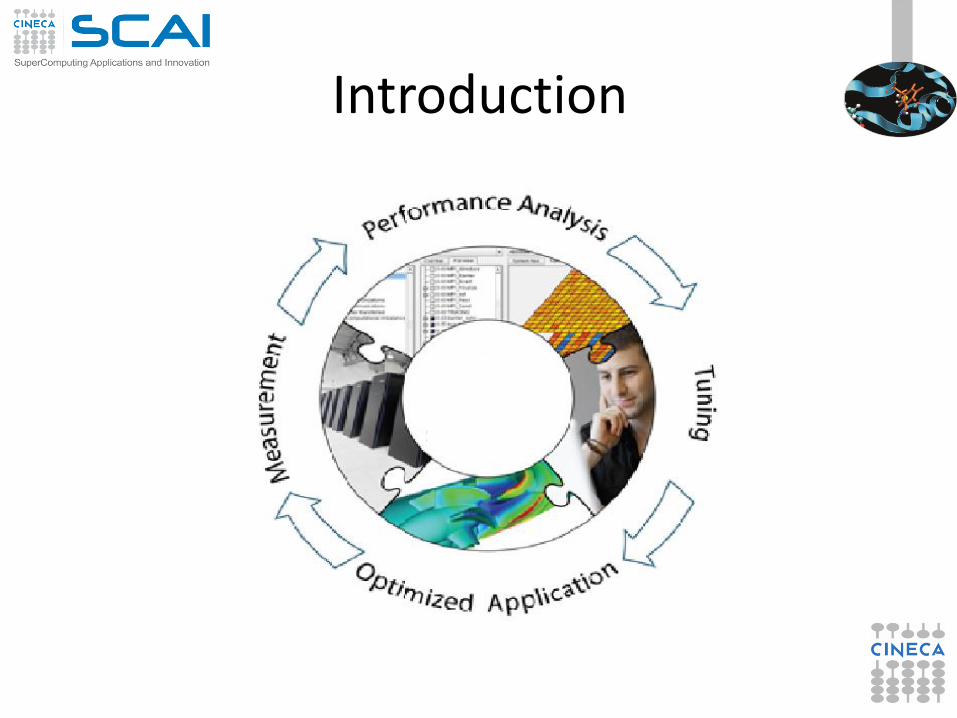
Introduction

A serial or parallel program is normally composed by a large number of procedures.

To optimize and parallelize a complex code is fundamental to find out the parts where most of time is spent.

Moreover is very important to understand the graph of computation and the dependencies and correlations between the different sections of the code.

For a good scalability in parallel programs, it’s necessary to have a good load and communication balancing between processes.

To discover the hotspots and the bottlenecks of a code and find out the best optimization and parallelization strategy the programmer can follow two common methods:

Manual instumentation inserting timing and collecting functions (difficult)

Automatic profiling using profilers (easier and very powerful)

Introduction

Measuring execution time

• Both C/C++ and Fortran programmers are used to instrument the code with timing and printing functions to measure and collect or visualize the time spent in critical or computationally intensive code’ sections.

Fortran77

etime(),dtime()

Fortran90

cputime(), system_clock(), date_and_time()

C/C++

clock()

• In this kind of operations it must be taken into account of:

Intrusivity

Granularity

Relaiability

Overhead

• Very difficult task for third party complex codes


C example:

#include <time.h>

clock_t time1, time2;

double dub_time;

…

time1 = clock();

for (i = 0; i < nn; i++)

for (k = 0; k < nn; k++)

for (j = 0; j < nn; j ++)

c[i][j] = c[i][j] + a[i][k]*b[k][j];

time2 = clock();

dub_time = (time2 - time1)/(double) CLOCKS_PER_SEC;

printf("Time -----------------> %lf \n", dub_time);


Fortran example: real(my_kind), intent(out) :: t

integer :: time_array(8)

…

call date_and_time(values=time_array)

t1 = 3600.*time_array(5)+60.*time_array(6)+time_array(7)+time_array(8)/1000.

do j = 1,n

do k = 1,n

do i = 1,n

c(i,j) = c(i,j) + a(i,k)*b(k,j)

enddo

enddo

enddo

call date_and_time(values=time_array)

t2 = 3600.*time_array(5)+60.*time_array(6)+time_array(7)+time_array(8)/1000.

write(6,*) t2-t1

Profilers

• There are many versions of commercial profilers, developed by manufacturers of compilers and specialized software house. In addition there are free

profilers, as those resulting from the GNU, TAU or Scalasca project.

Tau Performance System

- University of Oregon

Scalasca

-Research Centre Juelich PGPROF

Intel® VTune™ Amplifier

OPT GNU gprof

PerfSuite

– National Center for Supercomputing Applications

Profilers

• Profilers allow the programmer to obtain very useful information on the various parts of a code with basically two levels of profiling:

• Subroutine/Function level

– Timing at routine/funcion level, graph of computation flow

– less intrusive

– Near realistic execution time

• Construct/instruction/statement level

– capability to profile each instrumented statement

– more intrusive

– very accurate timing information

– longer profiling execution time

GNU Profiler

• The GNU profiler “gprof” is an open-source tool that allows profiling of serial and parallel codes.

• GNU profiler how to:

– Recompile source code using compiler profiling flag: gcc –pg source code

g++ -pg source code

gfortran –pg source code

– Run the executable to allow the generation of the files containing profiling information:

o At the end of the execution in the working directory will be generated a specific file generally named “gmon.out” containing all the analytic information for the profiler

– Results analysis gprof executable gmon.out

GNU Profiler

Code is automatically instrumented by the compiler when using the –pg flag, during the execution:

– the number of calls and the execution time of each subroutine is collected

– a call graph containing dependences between subroutines is implemented

– a binary file containing above information is generated (gmon.out)

The profiler, using data contained in the file gmon.out, is able to give precise information about:

1. the number of calls of each routine

2. the execution time of a routine

3. the execution time of a routine and all the child routines called by that routine

4. a call graph profile containing timing information and relations between subroutines

Gnu Profiler

double add3(double x){

return x+3;

}

double mysum(double *a, int n){

double sum=0.0;

for(int i=0;i<n;i++)

sum+=a[i]+add3(a[i]);

return sum;

}

double init(double *a,int n){

double res;

for (int i=0;i<n;i++) a[i]=double(i);

res=mysum(a,n);

return res;

}

Example

int main(){

double res,mysum;

int n=1000;

double a[n];

for (int i=0;i<n;i++){

res=init(a,n);

}

printf("Result %f\n",res);

return 0;

}

Profiler output

• The profiler gprof produces two kinds of statistical output: “flat profile” and “call graph profile”.

• According to previous example flat profile gives the following information:

Flat profile:

Each sample counts as 0.01 seconds.

% cumulative self self total

time seconds seconds calls us/call us/call name

48.60 0.41 0.41 10000 41.31 81.61 init(double*, int)

27.26 0.64 0.23 10000 23.17 40.30 mysum(double*, int)

20.15 0.82 0.17 100000000 0.00 0.00 add3(double)

3.56 0.85 0.03 frame_dummy

Flat profile

The meaning of the columns displayed in the flat profile is:

• % time: percentage of the total execution time your program spent in this function

• cumulative seconds: cumulative total number of seconds the computer spent executing this functions, plus the time spent in all the functions above this one in this table

• self seconds: number of seconds accounted for by this function alone.

• calls: total number of times the function was called

• self us/calls: represents the average number of microseconds spent in this function per call

• total us/call: represents the average number of microseconds spent in this function and its descendants per call if this function is profiled, else blank

• name: name of the function

Call Graph

• Call Graph Profile: gives more detailed timing and calling sequence information through a dependency call graph.

Call graph (explanation follows)

index % time self children called name

<spontaneous>

[1] 96.4 0.00 0.82 main [1]

0.41 0.40 10000/10000 init(double*, int) [2]

-----------------------------------------------

0.41 0.40 10000/10000 main [1]

[2] 96.4 0.41 0.40 10000 init(double*, int) [2]

0.23 0.17 10000/10000 mysum(double*, int) [3]

Call Graph

-----------------------------------------------

0.23 0.17 10000/10000 init(double*, int)

[2]

[3] 47.6 0.23 0.17 10000 mysum(double*, int) [3]

0.17 0.00 100000000/100000000 add3(double) [4]

-----------------------------------------------

0.17 0.00 100000000/100000000 mysum(double*,

int) [3]

[4] 20.2 0.17 0.00 100000000 add3(double) [4]

-----------------------------------------------

<spontaneous>

[5] 3.6 0.03 0.00 frame_dummy [5]

-----------------------------------------------

Line level profiling

If necessary it’s possible to profile single lines or blocks of code with the GNU profiler used together with the “gcov” tool to see:

– lines that are most frequently accessed

– computationally critical statements or regions

Line level profiling with gcov requires the following steps

– compile with -fprofile-arcs -ftest-coverage At the end of compilation files *.gcno will be produced

– Run the executable. The execution will produce *.gcda files

– Run gcov: gcov [options] sourcefiles

– At the end of running in the working directory will be present a specific file with extension *.gcov which contains all the analytic information for the profiler

NOTES:

- gcov is compatible only with code compiled with GNU compilers

- use low level optimization flags.

Example

C example

#include <stdlib.h>

#include <stdio.h>

int prime (int num);

int main()

{

int i,cnt=0;

for (i=2; i <= 1000000; i++)

if (prime(i)) {

cnt++;

if (cnt%9 == 0) {

printf("%5d\n",i);

cnt = 0;

}

else

printf("%5d ", i);

}

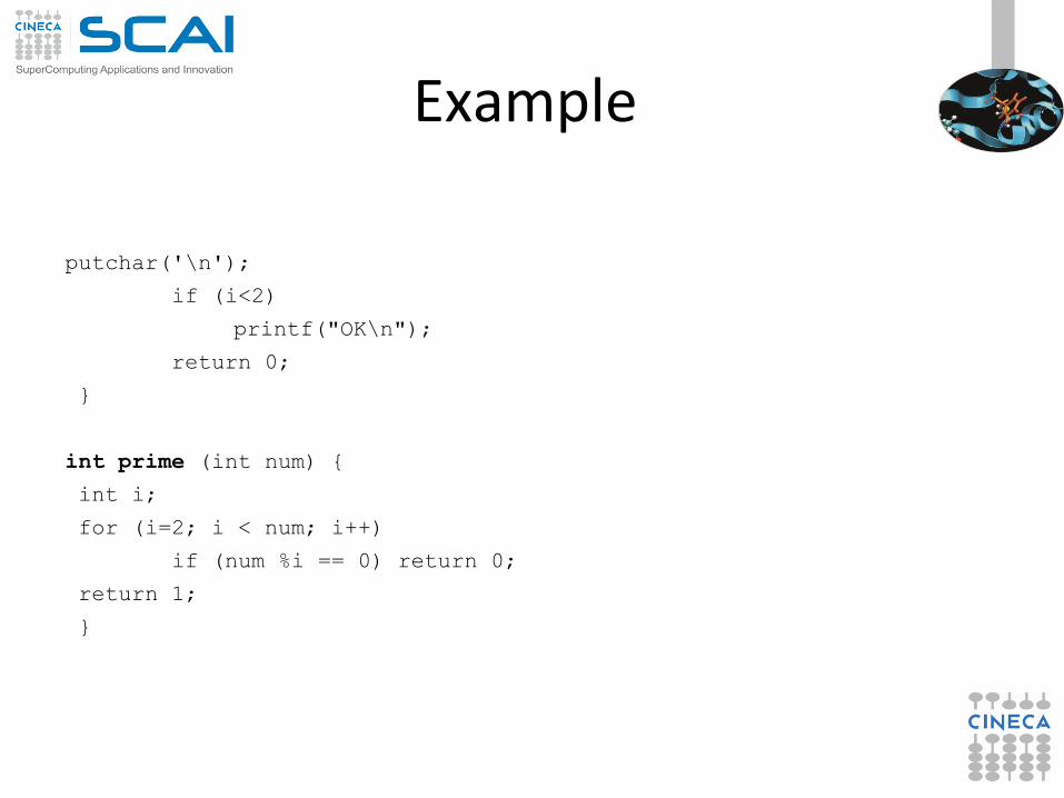
Example

putchar('\n');

if (i<2)

printf("OK\n");

return 0;

}

int prime (int num) {

int i;

for (i=2; i < num; i++)

if (num %i == 0) return 0;

return 1;

}

Example

Routine level profiling produces the following information:

Each sample counts as 0.01 seconds.

% cumulative self self total

time seconds seconds calls us/call us/call name

100.99 109.74 109.74 999999 109.74 109.74 prime(int)

Granularity: each sample hit covers 2 byte(s) for 0.01% of 109.74 seconds

index % time self children called name

<spontaneous>

[1] 100.0 0.00 109.74 main [1]

109.74 0.00 999999/999999 prime(int) [2]

-----------------------------------------------

109.74 0.00 999999/999999 main [1]

[2] 100.0 109.74 0.00 999999 prime(int) [2]

Example

-: 1:#include <stdlib.h>

-: 2:#include <stdio.h>

-: 3:

-: 4:int prime (int num);

-: 5:

1: 6:int main()

-: 7: {

-: 8: int i;

1: 9: int cnt = 0;

1000000: 10: for (i=2; i <= 1000000; i++)

999999: 11: if (prime(i)) {

78498: 12: cnt++;

78498: 13: if (cnt%9 == 0) {

8722: 14: printf("%5d\n",i);

8722: 15: cnt = 0;

-: 16: }

-: 17: else

69776: 18: printf("%5d ", i);

Example

-: 19: }

1: 20: putchar('\n');

1: 21: if (i<2)

#####: 22: printf("OK\n");

1: 23: return 0;

-: 24: }

-: 25:

999999: 26:int prime (int num) {

-: 27: /* check to see if the number is a prime? */

-: 28: int i;

37567404990: 29: for (i=2; i < num; i++)

37567326492: 30: if (num %i == 0) return 0;

78498: 31: return 1;

-: 32: }

Example

Line level profiling shows that most of time is spent in the for loop and in the if construct contained in the prime function.

That portion of code can be written in a more efficient way.

int prime (int num) {

/* check to see if the number is a prime? */

int i;

for (i=2; i <= faster(num); i++)

if (num %i == 0)

return 0;

return 1;

}

int faster (int num)

{

return (int) sqrt( (float) num);

}

Example

1: 7:int main(){

-: 8: int i;

1: 9: int colcnt = 0;

1000000: 10: for (i=2; i <= 1000000; i++)

999999: 11: if (prime(i)) {

78498: 12: colcnt++;

78498: 13: if (colcnt%9 == 0) {

8722: 14: printf("%5d\n",i);

8722: 15: colcnt = 0;

-: 16: }

-: 17: else

69776: 18: printf("%5d ", i);

-: 19: }

Example

1: 20: putchar('\n');

1: 21: return 0;

-: 22: }

-: 23:

999999: 24: int prime (int num) {

-: 25: int i;

67818902: 26: for (i=2; i <= faster(num); i++)

67740404: 27: if (num %i == 0)

921501: 28: return 0;

78498: 29: return 1;

-: 30: }

-: 31:

67818902: 32: int faster (int num)

-: 33: {

67818902: 34: return (int) sqrt( (float) num);

-: 35: }

Results

0.96 sec Vs 109.67 sec

10^7 operations VS

10^10 operations

gprof execution time impact

• Routine level and above all line level profiling can cause a certain overhead in execution time:

• Travelling Salesman Problem (TSP):

g++ -pg –o tsp_prof tsp.cc

g++ -o tsp_no_prof tsp.cc

• Execution time time ./TSP.noprof

10.260u 0.000s 0:10.26 100.0%

time ./TSP.prof

15.480u 0.020s 0:15.87 97.6%

Be careful when you have to choose input dataset and configuration for profiling

Real case Air Pollution Model • Model structure and call graph

• Fluid dynamics equations are solved over a 3D grid

cgae (main)

Setup

Comp ( contains the

main loop over time steps

end calls computing and

I/O routines)

Minor computing

routines

Opspltae

Output

Units

Horizae

Horizae

Units

Ztrans

Phfact

Chemnew

Aero_iso

Loop 500 over

X-Y grid cells

Fin (finalization)

Loop over time steps (24

time steps in a day of

simulation)

Real case air pollution model

• Profiling with GNU profiler (call graph)

• 1 day of simulation. Only the computationally intensive routines of the model are shown

• 5 days of simulation. Only the computationally intensive routines of the

model are shown

Real case air pollution model parallelization strategy

Dependency call graph of “opspltae” routine


• Opspltae:

– The most computationally intensive part of this routine is Loop 500 which contains calls to ztrans, phfact, chemnew,aero_iso routines which work on a single X,Y point of the 3D grid with no communication, so can be called in parallel by each MPI process.

– The operations in Loop 500 are indipendent along X,Y direction domain can be decomposed along X or Y.

– At the end of the loop 500

communication is required because some matrices must be gathered by master process and broadcasted to other MPI processes.

Minor computing

routines

Opspltae

Output

Units

Horizae

Horizae

Units

Ztrans

Phfact

Chemnew

Aero_iso

Loop 500



simulation)


• Horizae: – This routine is responsible for the transport

along X,Y directions. It’s called in opspltae before and after Loop 500. It receives in input the entire 3D grid and integrates respectively in the X and Y dimension.

– During integration in the X dimension domain is decomposed in the Y direction and vice versa.

– Between the two integration phases communication of some matrices is required and at the end of the routine the master must receive all the partial contributes by others MPI processes.

Results

Real speedup : 7.6

Why?

Minor computing

routines

Opspltae

Output

Units

Horizae

Horizae

Units

Ztrans

Phfact

Chemnew

Aero_iso

Loop 500



simulation)

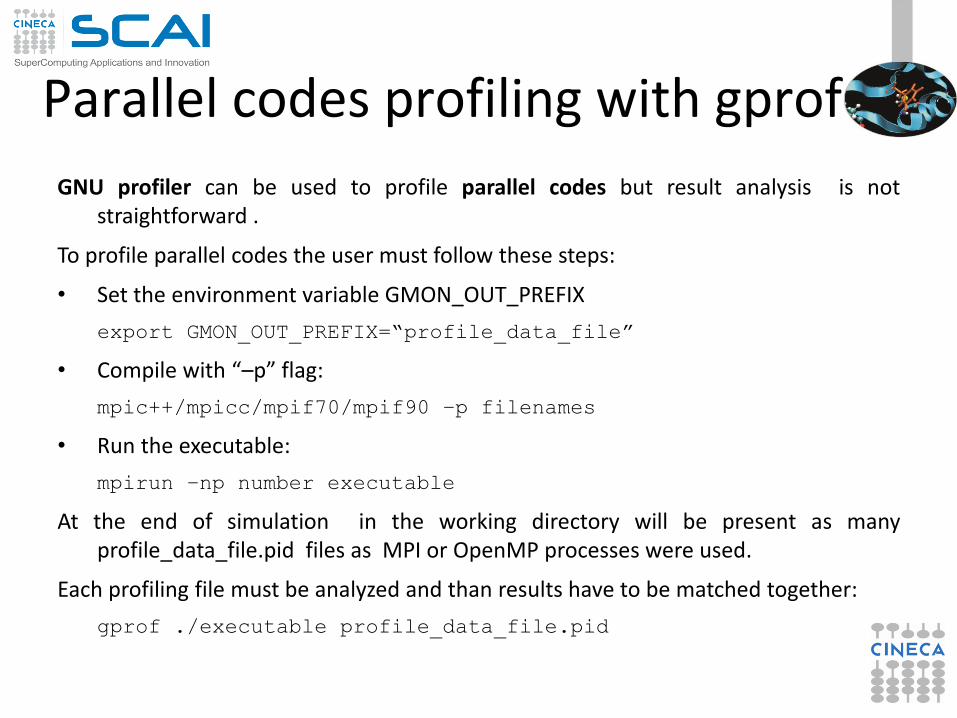
Parallel codes profiling with gprof

GNU profiler can be used to profile parallel codes but result analysis is not straightforward .

To profile parallel codes the user must follow these steps:

• Set the environment variable GMON_OUT_PREFIX

export GMON_OUT_PREFIX=“profile_data_file”

• Compile with “–p” flag:

mpic++/mpicc/mpif70/mpif90 –p filenames

• Run the executable:

mpirun –np number executable

At the end of simulation in the working directory will be present as many profile_data_file.pid files as MPI or OpenMP processes were used.

Each profiling file must be analyzed and than results have to be matched together:

gprof ./executable profile_data_file.pid

TAU Tuning and Analysis Utilities

• TAU Performance System® is a portable profiling and tracing toolkit for performance analysis of serial and parallel programs written in Fortran, C, C++, Java, and Python.

www.cs.uoregon.edu/research/tau

• 12+ years of project in which are currently involved:

– University of Oregon Performance Research Lab

– LANL Advanced Computing Laboratory

– Research Centre Julich at ZAM, Germany

• TAU (Tuning and Analysis Utilities) is capable of gathering performance information through instrumentation of functions, methods, basic blocks and statements of serial and shared or distributed memory parallel codes

• It’s portable on all architectures

• Provides powerful and user friendly graphic tools for result analysis

http://www.cs.uoregon.edu/research/tau

http://www.cs.uoregon.edu/research/tau

TAU: architecture

TAU Installation and configuration

During the installation phase TAU requires different configurations flags depending on the kind of code to be analyzed.

• After configuration TAU can be easily installed with: • make • make install

TAU: introduction

• TAU provides three different methods to track the performance of your application.

• The simplest way is to use TAU with dynamic instrumentation based on pre-charged libraries

Dynamic instrumentation

• Doesn’t requires to recompile the executable

• Instrumentation is achieved at run-time through library pre-loading

• Dynamic instrumentation include tracking MPI, io, memory, cuda, opencl library calls. MPI instrumentation is included by default, the others are enabled by command-line options to tau_exec.

– Serial code

%> tau_exec -io ./a.out

– Parallel MPI code

%> mpirun -np 4 tau_exec -io ./a.out

– Parallel MPI + OpenMP code

%> mpirun –x OMP_NUM_THREADS=2 -np 4 tau_exec -io

./a.out

TAU: Compiler based instrumentation

• For more detailed profiles, TAU provides two means to compile your application with TAU: through your compiler or through source transformation using PDT.

• It’s necessary to recompile the application, static instrumentation at compile time

• TAU provides these scripts to instrument and compile Fortran, C,and C++ programs respectively:

– tau_f90.sh

– tau_cc.sh

– tau_cxx.sh

• Compiler based instrumentation needs the following steps:

– Environment configuration

– Code recompiling

– Execution

– Result analysis

TAU: Compiler based instrumentation

1. Environment configuration:

%>export TAU_MAKEFILE=[path to tau]/[arch]/lib/[makefile]

%>export TAU_OPTIONS=‘-optCompInst –optRevert’

Optional:

%>export PROFILEDIR = [path to directory with result]

2. Code recompiling:

%>tau_cc.sh source_code.c

3. To enable callpath creation:

%>export TAU_CALLPATH=1

%>export TAU_CALLPATH_DEPTH=30

4. To enable MPI message statistics

%>export TAU_TRACK_MESSAGE=1

TAU environment variables

Environment Variable Default Description

TAU_PROFILE 0 Set to 1 to have TAU profile your code

TAU_CALLPATH 0 When set to 1 TAU will generate call-path data. Use with TAU_CALLPATH_DEPTH.

TAU_TRACK_MEMORY_LEAKS

0 Set to 1 for tracking of memory leaks (to be used with tau_exec –memory)

TAU_TRACK_HEAP or TAU_TRACK_HEADROOM

0 Setting to 1 turns on tracking heap memory/headroom at routine entry & exit using context events (e.g., Heap at Entry: main=>foo=>bar)

TAU_CALLPATH_DEPTH 2 Callapath depth. 0 No callapath. 1 flat profile

TAU_SYNCHRONIZE_CLOCKS

1 When set TAU will correct for any time discrepancies between nodes because of their CPU clock lag.

TAU_COMM_MATRIX 0 If set to 1 generate MPI communication matrix data.

TAU_THROTTLE 1 If set to 1 enables the runtime throttling of events that are lightweight

TAU_THROTTLE_NUMCALLS

100000 Set the maximum number of calls that will be profiled for any function when TAU_THROTTLE is enabled

TAU_THROTTLE_PERCALL

10 Set the minimum inclusive time (in milliseconds) a function has to have to be instrumented when TAU_THROTTLE is enabled.

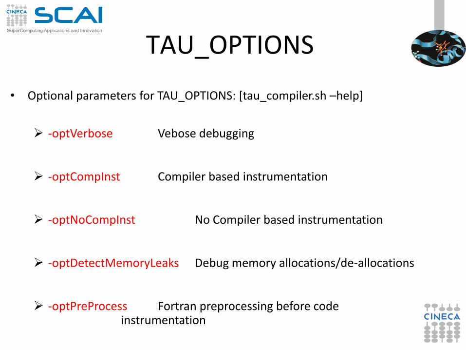
TAU_OPTIONS

• Optional parameters for TAU_OPTIONS: [tau_compiler.sh –help]

-optVerbose Vebose debugging

-optCompInst Compiler based instrumentation

-optNoCompInst No Compiler based instrumentation

-optDetectMemoryLeaks Debug memory allocations/de-allocations

-optPreProcess Fortran preprocessing before code instrumentation

-optTauSelectFile="" Selective file for the tau_instrumentor

Result analysis • At the end of a run, a code instrumented with TAU produces a series of files

“profile.x.x.x” containing the profiling information.

• TAU provides two tools for profiling analysis :

– pprof command line, useful for a quick view summary of TAU performance

– Paraprof with a sophisticated GUI allows very detailed and powerful analysis

• Usage: pprof [-c|-b|-m|-t|-e|-i|-v] [-r] [-s] [-n num] [-f filename] [-p] [-l] [-d] [node numbers]

-a : Show all location information available

-c : Sort according to number of Calls

-b : Sort according to number of suBroutines called by a function

-m : Sort according to Milliseconds (exclusive time total)

-t : Sort according to Total milliseconds (inclusive time total) (default)

-e : Sort according to Exclusive time per call (msec/call)

-i : Sort according to Inclusive time per call (total msec/call)

-v : Sort according to Standard Deviation (excl usec)

-r : Reverse sorting order

-s : print only Summary profile information

-n <num> : print only first <num> number of functions

-f filename : specify full path and Filename without node ids

-p : suPpress conversion to hh:mm:ss:mmm format

-l : List all functions and exit

-d : Dump output format (for tau_reduce) [node numbers] : prints only info about all contexts/threads of given node numbers

Result analysis: paraprof

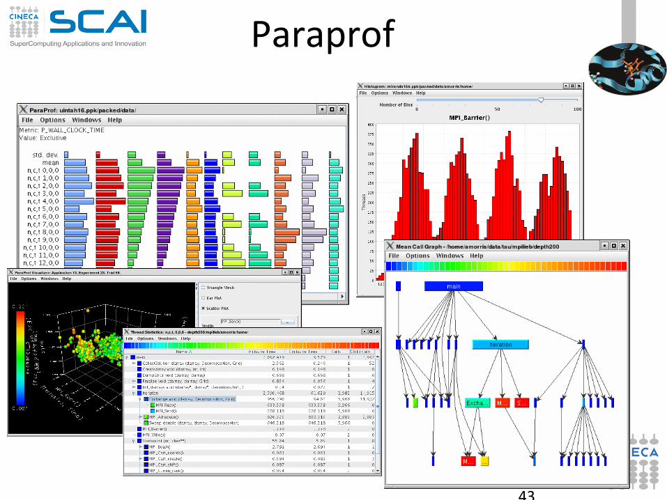
43

Paraprof

Example #include<stdio.h>

double add3(double x){

return x+3;}

double mysum(double *a, int n){

double sum=0.0;

for(int i=0;i<n;i++)

sum+=a[i]+add3(a[i]);

return sum;

}

double init(double *a,int n){

double res;

for (int i=0;i<n;i++) a[i]=double(i);

res=mysum(a,n);

return res;

}

int main(){

double res,mysum;

int n=30000;

double a[n];

for (int i=0;i<n;i++){

res=init(a,n);

}

printf("Result %f\n",res);

return 0;}

Pprof pprof output:

%> pprof

Reading Profile files in profile.*

NODE 0;CONTEXT 0;THREAD 0:

-------------------------------------------------------------------------------

%Time Exclusive Inclusive #Call #Subrs Inclusive Name

msec total msec usec/call

-------------------------------------------------------------------------------

100.0 3 3:20.342 1 1 200342511 .TAU application

100.0 4 3:20.338 1 30000 200338851 main

100.0 2,344 3:20.334 30000 30000 6678 init

98.8 1:40.824 3:17.989 30000 9E+08 6600 mysum

48.5 1:37.164 1:37.164 9E+08 0 0 add3

46

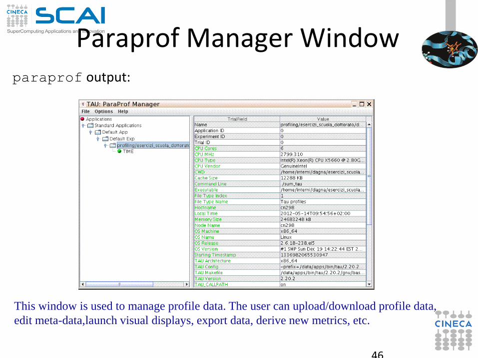
Paraprof Manager Window paraprof output:

This window is used to manage profile data. The user can upload/download profile data,

edit meta-data,launch visual displays, export data, derive new metrics, etc.

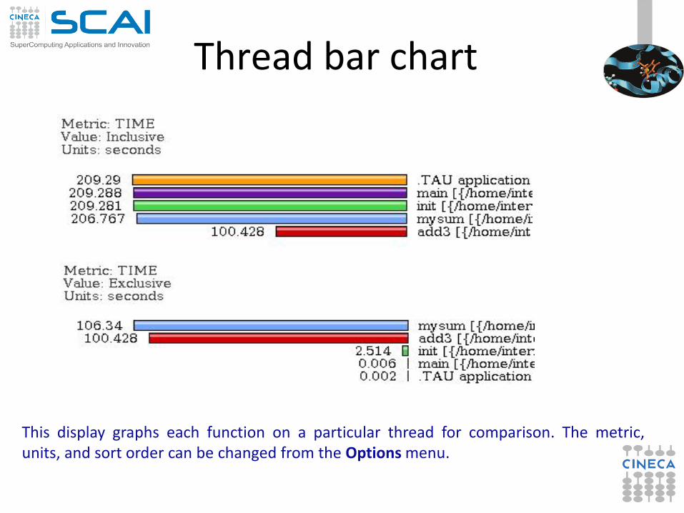
Thread bar chart

This display graphs each function on a particular thread for comparison. The metric, units, and sort order can be changed from the Options menu.

Call Graph

• This display shows callpath data in a graph using two metrics, one determines the width, the other the color.

• The full name of the function as well as

the two values (color and width) are displayed in a tooltip when hovering over a box.

• By clicking on a box, the actual ancestors

and descendants for that function and their paths (arrows) will be highlighted with blue.

• This allows you to see which functions are

called by which other functions since the interplay of multiple paths may obscure it.

Thread Call Path Relations Window

For example “mysum” is called from “init” 30000 times for a total of 64.5 seconds and calls “add3” function. TAU automatically throttles short running functions in an effort to reduce the amount of overhead associated with profiles of such functions, default throttle limit is: numcalls> 100000 && usecs/call < 10

To change default settings TAU gives the following environment variables: TAU_THROTTLE_NUMCALLS, TAU_THROTTLE_PERCALL

To disable TAU throttle : export TAU_THROTTLE=0

Thread Statistics Table

This display shows the callpath data in a table. Each callpath can be traced from root to leaf by opening each node in the tree view. A colorscale immediately draws attention to "hot spots" areas that contain highest values.

Tau profiler: parallel codes

TAU provides a lot of tools to analyze OpenMP, MPI or OpenMP + MPI parallel codes.

Profiling the application the user can obtain a lot of useful information which can help to identify the causes of an unexpected low parallel efficiency.

Principal factors which can affect parallel efficiency are:

– load balancing

– communication overhead

– process synchronization

– Latency and bandwidth

Tau profiler: parallel codes

• Configure:

%>export TAU_MAKEFILE=[path to

tau]/[arch]/lib/[makefile]

%>export TAU_OPTIONS=-optCompInst

• Compile:

Tau_cc.sh –o executable source.c (C)

Tau_cxx.sh –o executable source.cpp (C++)

Tau_f90.sh –o executable source.f90 (Fortran)

• Run the application:

mpirun -np #procs ./executable

At the end of simulation, in the working directory or in the path specified with the PROFILEDIR variable, the data for the profiler will be saved in files profile.x.x.x

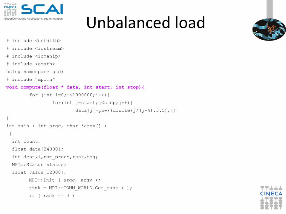
Unbalanced load # include <cstdlib>

# include <iostream>

# include <iomanip>

# include <cmath>

using namespace std;

# include "mpi.h"

void compute(float * data, int start, int stop){

for (int i=0;i<1000000;i++){

for(int j=start;j<stop;j++){

data[j]=pow((double)j/(j+4),3.5);}}

}

int main ( int argc, char *argv[] )

{

int count;

float data[24000];

int dest,i,num_procs,rank,tag;

MPI::Status status;

float value[12000];

MPI::Init ( argc, argv );

rank = MPI::COMM_WORLD.Get_rank ( );

if ( rank == 0 )

Unbalanced load {

num_procs = MPI::COMM_WORLD.Get_size ( );

cout << " The number of processes available is " << num_procs << "\n";

}

if ( rank == 0 )

{

tag = 55;

MPI::COMM_WORLD.Recv ( value,12000, MPI::FLOAT, MPI::ANY_SOURCE, tag,

status );

cout << "P:" << rank << " Got data from process " <<

status.Get_source() << "\n";

count = status.Get_count ( MPI::FLOAT );

cout << "P:" << rank << " Got " << count << " elements.\n";

compute(value,0,12000);

}

Unbalanced load else if ( rank == 1 )

{

cout << "\n";

cout << "P:" << rank << " - setting up data to send to process 0.\n";

for ( i = 0; i <24000; i++ )

{

data[i] = i;

}

dest = 0;

tag = 55;

MPI::COMM_WORLD.Send ( data, 12000, MPI::FLOAT, dest, tag );

compute(data,12000,24000);

}else{

cout << "\n";

cout << "P:" << rank << " - MPI has no work for me!\n";

}

MPI::Finalize ( );

if ( rank == 0 )

{

cout << " Normal end of execution.\n";

}

return 0;

}

Unbalanced load

Output:

The number of processes available is 4

P:0 Got data from process 1

P:0 Got 12000 elements.

P:1 - setting up data to send to process 0.

P:3 - MPI has no work for me!

P:2 - MPI has no work for me!

Normal end of execution.

Unstacked bars

Very useful to compare individual functions across threads in a global display

Comparison window

Very useful to compare the behavior of process and threads in all the functions or regions of the code to find load unbalances.

3D Visualizer

This visualization method shows two metrics for all functions, all threads. The height represents one chosen metric, and the color, another. These are selected from the drop-down boxes on the right.

To pinpoint a specific value in the plot, move the Function and Thread sliders to cycle

through the available functions/threads.

MPI_Finalize()

MPI_Init()

compute()

Balanced load Balancing the load: int main ( int argc, char *argv[] )

{

MPI::Init ( argc, argv );

rank = MPI::COMM_WORLD.Get_rank ( );

float data[24000];

if ( rank == 0 )

{

num_procs = MPI::COMM_WORLD.Get_size ( );

cout << " The number of processes available is " << num_procs << "\n";

}

int subd = 24000/num_procs

if ( rank!= 0)

{

tag = 55;

MPI::COMM_WORLD.Recv ( data,subd, MPI::FLOAT, MPI::ANY_SOURCE, tag, status );

cout << "P:" << rank << " Got data from process " <<

status.Get_source() << "\n";

count = status.Get_count ( MPI::FLOAT );

cout << "P:" << rank << " Got " << count << " elements.\n";

compute(data,rank*subd,rank*subd+subd);

printf("Done\n");

}

Balanced load else if ( rank == 0 )

{

cout << "\n";

cout << "P:" << rank << " - setting up data to send to processes.\n";

for ( i = 0; i <24000; i++ )

{

data[i] = i;

}

tag = 55;

printf("Done\n");

for(int el=1;el<num_procs;el++){

MPI::COMM_WORLD.Send ( &data[subd*el], subd, MPI::FLOAT, el, tag );

}

compute(data,0,subd);

}

MPI::Finalize ( );

if ( rank == 0 )

{

cout << " Normal end of execution.\n";

}

return 0;

}

Balanced load • Output: The number of processes available is 6

P:0 - setting up data to send to processes.

Done











Done

Done

Done

Done

Done

Normal end of execution.

Balanced load

MPI_Finalize()

MPI_Init()

compute()

Real Case Air Pollution Model

Inclusive Exclusive Calls/Tot.Calls

Metric: TIME Sorted By: Exclusive Units: seconds

Minor computing

routines

Opspltae

Output

Units

Horizae

Horizae

Units

Ztrans

Phfact

Chemnew

Aero_iso

Loop 500

Loop over time steps


Amdahl law Theoretical speedup

P=0.93 S(N)=14

Real speedup = 7.6

Let’s check communication and load balncing !!


Master process Slave processes

Load balancing issues Communication issues

The imbalance of computational load causes an overhead in the MPI directives due to long synchronization times dramatically reducing the scalability

TAU Instrumentation API

• Using the specific API with TAU it’s possible to obtain a very detailed profiling of your code.

• Code instrumentation based on the API can be done authomatically or manually. With manual code instrumentation the programmer can establish exactly which sections are to be profiled and how.

• TAU API is available for C++, C and Fortran77/90/95 codes and is portable among different platforms and compilers.

• To use the API at the beginning of each source to be profiled must be present the line: #include<TAU.h>

• Most important API capabilities:

– Routines profiling

– Blocks or lines profiling

– Heap-memory tracing

TAU Instrumentation API • Configuration and Initialization:

– At the beginning of each instrumented source file, include the header “TAU.h”

TAU_PROFILE_INIT(argc, argv);

TAU_PROFILE_SET_NODE(myNode);

• Class funcitions and methods (C++ only):

TAU_PROFILE(name, type, group);

• User-defined timing

TAU_PROFILE_TIMER(timer, name, type, group);

TAU_PROFILE_START(timer);

TAU_PROFILE_STOP(timer);

• Heap-memory tracing:

TAU_TRACK_MEMORY();

TAU_SET_INTERRUPT_INTERVAL(seconds);

C++ example #include <TAU.h>

int foo();

int main(int argc, char **argv)

{

TAU_PROFILE("int main(int, char **)","", TAU_DEFAULT);

TAU_PROFILE_INIT(argc, argv);

TAU_PROFILE_SET_NODE(0); /* just for serial programs */

int cond=foo();

return 0;

}

int foo()

{

int N=100000;

double a[N];

int cond=0;

TAU_PROFILE("int foo(void)","", TAU_DEFAULT); // routine level profiling foo()

TAU_PROFILE_TIMER(t,"foo(): for loop", "[22:29 file.cpp]", TAU_USER);

TAU_PROFILE_START(t);

for(int i = 0; i < N ; i++){

a[i]=i/2;

if (i%2 ==0) cond=0;

else cond=1;

}

TAU_PROFILE_STOP(t);

if (cond==1) return 25;

else return 15;}

Example

With manual instrumentation using the API we can see detailed statistic

information on a specific block of code

Fortran example PROGRAM SUM_OF_CUBES

integer profiler(2)

save profiler

INTEGER :: H, T, U

call TAU_PROFILE_INIT()

call TAU_PROFILE_TIMER(profiler, 'PROGRAM SUM_OF_CUBES')

call TAU_PROFILE_START(profiler)

call TAU_PROFILE_SET_NODE(0)

! This program prints all 3-digit numbers that

! equal the sum of the cubes of their digits.

DO H = 1, 9

DO T = 0, 9

DO U = 0, 9

IF (100*H + 10*T + U == H**3 + T**3 + U**3) THEN

PRINT "(3I1)", H, T, U

ENDIF

END DO

END DO

END DO

call TAU_PROFILE_STOP(profiler)

END PROGRAM SUM_OF_CUBES

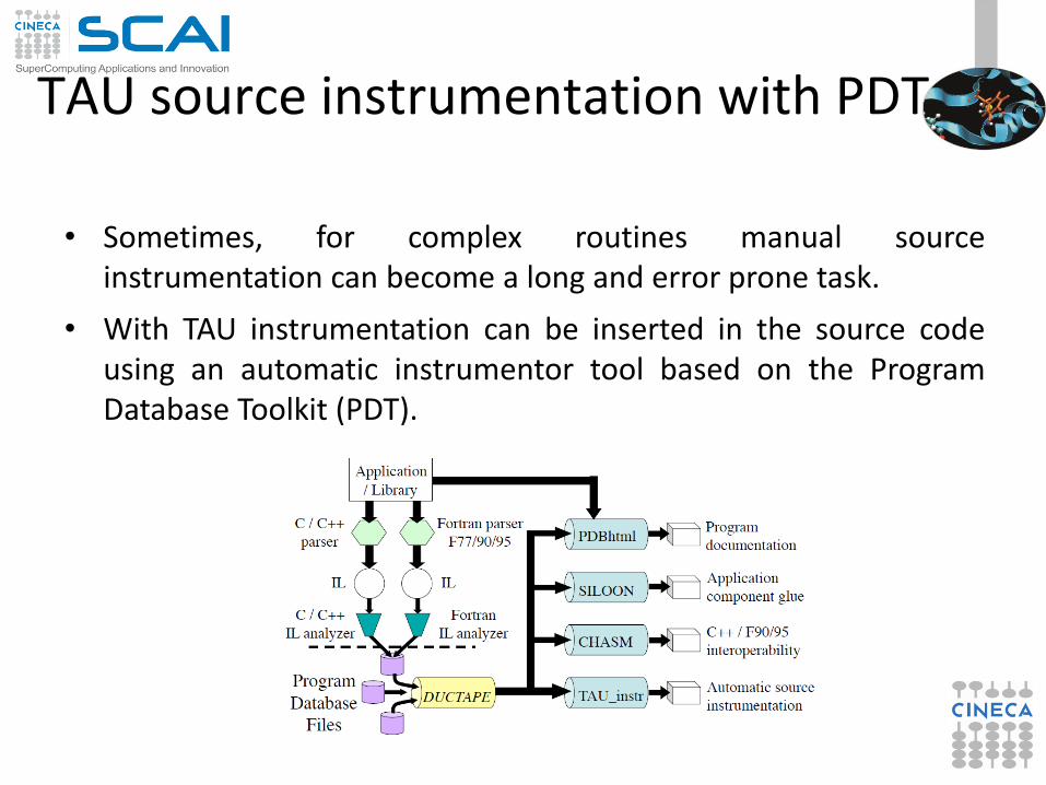
TAU source instrumentation with PDT

• Sometimes, for complex routines manual source instrumentation can become a long and error prone task.

• With TAU instrumentation can be inserted in the source code using an automatic instrumentor tool based on the Program Database Toolkit (PDT).


TAU and PDT howto:

• Parse the source code to produce the .pdb file:

– cxxparse file.cpp C++

– cparse file.c C

– f95parse file.f90 Fortran

• Instrument the program:

– tau_instrumentor file.pdb file.cpp –o

file.inst.cpp –f select.tau

• Complile:

– tau_compiler.sh file.inst.cpp –o file.exe


• The ”-f” flag associated to the command “tau_instrumentator” allows you to customize the instrumentation of a program by using a selective instrumentation file. This instrumentation file is used to manually control which parts of the application are profiled and how they are profiled.

• Selective instrumentation file can contain the following sections:

1. Routines exclusion/inclusion list:

BEGIN_EXCLUDE_LIST / END_EXCLUDE_LIST

BEGIN_INCLUDE_LIST / END_INCLUDE_LIST

2. Files exclusion/inclusion list:

BEGIN_FILE_EXCLUDE_LIST / END_FILE_EXCLUDE_LIST

BEGIN_FILE_INCLUDE_LIST / END_FILE_INCLUDE_LIST

3. More detailed instrumentation specifics:

BEGIN_INSTRUMENT_SECTION / END_INSTRUMENT_SECTION


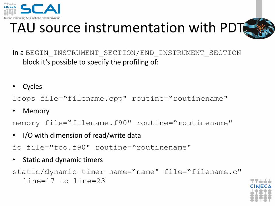
In a BEGIN_INSTRUMENT_SECTION/END_INSTRUMENT_SECTION block it’s possible to specify the profiling of:

• Cycles

loops file=“filename.cpp" routine=“routinename"

• Memory

memory file=“filename.f90" routine=“routinename"

• I/O with dimension of read/write data

io file="foo.f90" routine=“routinename"

• Static and dynamic timers

static/dynamic timer name=“name" file=“filename.c"

line=17 to line=23

TAU with PDT Real Case Air Pollution Model

Custom profiling

Instrumentation file : instrument_rules.txt

-------------------------------------

BEGIN_FILE_INCLUDE_LIST

opspltae.f

chemnew.f

horizae.f

ztrans.f

END_FILE_INCLUDE_LIST

BEGIN_INSTRUMENT_SECTION

loops file="opspltae.f" routine="OPSPLTAE"

loops file="chemnew.f" routine="CHEMNEW"

loops file="horizae.f" routine="HORIZAE"

loops file="ztrans.f" routine="ZTRANS"

io file="wrout1.f" routine="WROUT1"

dynamic timer name="dyn_timer" file="opspltae.f" line=183 to line=189

END_INSTRUMENT_SECTION

--------------------------------------

Minor computing

routines

Opspltae

Output

Units

Horizae

Horizae

Units

Ztrans

Phfact

Chemnew

Aero_iso

Loop 500

Loop over time steps


Routine opspltae: Loop 500, TAU automatic instrumentation

call TAU_PROFILE_TIMER(profiler, 'OPSPLTAE [{opspltae.f} {2,18}]')

call TAU_PROFILE_START(profiler)

call TAU_PROFILE_TIMER(t_131, ' Loop: OPSPLTAE [{opspltae.f} {131,7}-{143,12}]')





iugrid= iaddrs('UGRID ',1,1,1,1,1)

…………

call TAU_PROFILE_START(t_247)

do 500 i=2,nxm1

do 500 j=2,nym1

.……………….

………………..

500 continue

call TAU_PROFILE_STOP(t_247)

TAU TIMER Initialization

TAU Loop 500 instrumentation

TAU Loop 500 end instrumentation


Profiling time with default routine level compiler based instrumentation : 4192 sec Profiling time with PDT and selective instrumentation : 1913 sec Execution time without profiling overhead: 1875 sec

TAU: Memory Profiling C/C++ TAU can evaluate the following memory events:

– how much heap memory is currently used

– how much a program can grow (or how much headroom it has) before it runs out of free memory on the heap

– Memory leaks (C/C++) TAU gives two main functions to evaluate memory:

– TAU_TRACK_MEMORY()

– TAU_TRACK_MEMORY_HERE() Esempio:

#include<TAU.h>

int main(int argc, char **argv) {

TAU_TRACK_MEMORY();

sleep(12);

double *x = new double[1024];

sleep(12);

return 0; }

TAU: Memory Profiling C/C++ NODE 0;CONTEXT 0;THREAD 0:

---------------------------------------------------------------------------------------

%Time Exclusive Inclusive #Call #Subrs Inclusive Name

msec total msec usec/call

---------------------------------------------------------------------------------------

100.0 20,002 20,002 1 0 20002086 int main(int, char **)

---------------------------------------------------------------------------------------

USER EVENTS Profile :NODE 0, CONTEXT 0, THREAD 0

---------------------------------------------------------------------------------------

NumSamples MaxValue MinValue MeanValue Std. Dev. Event Name

---------------------------------------------------------------------------------------

2 31.92 23.8 27.86 4.062 Memory Utilization (heap, in KB)

---------------------------------------------------------------------------------------

In the same way for the functions:

TAU_TRACK_MEMORY_HEADROOM()

TAU_TRACK_MEMORY_HEADROOM_HERE()

TAU: Memory Profiling Fortran To profile memory usage in Fortran 90 use TAU's ability to selectively instrument a program. The option -optTauSelectFile=<file> for tau_compilier.sh let you specify a selective instrumentation file which defines regions of the source code to instrument.

To begin memory profiling, state which file/routines to profile by typing:

BEGIN_INSTRUMENT_SECTION

memory file=“source.f90” routine=“routine_name”

END_INSTRUMENT_SECTION

Memory Profile in Fortran gives you these three metrics:

– Total size of memory for each malloc and free in the source code

– The callpath for each occurrence of malloc or free

– A list of all variable that were not deallocated in the source code.

Memory Hierarchy

DISK

RAM

L2 CACHE

L1 CACHE

REGISTER Speed Distance from

processors

Memory Size

Research

flow

Hit and Miss

• Hit: the processor immediately reads or writes the data in the cache line

• Miss: the cache allocates a new entry, and copies in data from main memory.

Hit rate: percentage of memory accesses which are satisfied by cache

Miss rate: 1 - hit rate

Hit time: Time to access cache

Miss Time: Time to replace a block in cache and deliver data

Performance Optimization

• Optimization of cache access can be helpful to improve code performance

• Optimization can be done at different stage:

- During compililation in order to reduce the instruction missing and the data missing

- Writing code in order to reduce spatial and time locality

Cache access can be analized through hardware counters and through profiling tools.

PAPI • Performance Api Programming Interface

• http://icl.cs.utk.edu/papi/

• PAPI is a set of API that can be used to access to the hardware counter information

• PAPI can be used with serial and parallel code

• PAPI can be used in two different way:

1. Low Level Interface

2. High Level Interface

http://icl.cs.utk.edu/papi/

http://icl.cs.utk.edu/papi/

PAPI:High Level

• Simple to use

• High level API

• 8 functions for C/C++ and Fortran.

PAPI_start_counters PAPI_stop_counters

PAPI_read_counters PAPI_accum_counters

PAPI_num_counters PAPI_ipc

PAPI_flips PAPI_flops

Example: #include "papi.h” #define NUM_EVENTS 2 long_long values[NUM_EVENTS];

unsigned int Events[NUM_EVENTS]={PAPI_TOT_INS,PAPI_TOT_CYC};

PAPI_start_counters((int*)Events,NUM_EVENTS);

do_work();

retval = PAPI_stop_counters(values,NUM_EVENTS);

PAPI Low Level

• Low level interface

• Increase granularity of information

• Hard to use

PAPI can be used integrated in many high level instruments:

• TAU (U Oregon) http://www.cs.uoregon.edu/research/tau/

• HPCToolkit (Rice Univ) http://hipersoft.cs.rice.edu/hpctoolkit/

• KOJAK (UTK, FZ Juelich) http://icl.cs.utk.edu/kojak/

• PerfSuite (NCSA) http://perfsuite.ncsa.uiuc.edu/

TAU & PAPI

• Before compiling configure TAU with the flag

-papi=directory_to_papi

• Verify events supported by your OS: papi_avail

PAPI Version : 4.1.2.1

Vendor string and code : GenuineIntel (1)

Model string and code : Intel(R) Xeon(R) CPU E7520 @ 1.87GHz (46)

CPU Revision : 6.000000

CPUID Info : Family: 6 Model: 46 Stepping: 6

CPU Megahertz : 1064.000000

CPU Clock Megahertz : 1064

Hdw Threads per core : 2

Cores per Socket : 4

NUMA Nodes : 8

CPU's per Node : 8

Total CPU's : 64

Number Hardware Counters : 7

Max Multiplex Counters : 512

TAU & PAPI • Checks metrics compatibility:

papi_event_chooser metrica1 metrica2 metricaN

./papi_event_chooser PAPI_FP_OPS PAPI_L1_DCM

Event Chooser: Available events which can be added with given events.

--------------------------------------------------------------------------------










NUMA Nodes : 8

CPU's per Node : 8

Total CPU's : 64



--------------------------------------------------------------------------------

Usage: papi_event_chooser NATIVE|PRESET evt1 evt2 ...

TAU & PAPI ./papi_event_chooser PAPI_FP_OPS GET_TIME_OF_DAY

Event Chooser: Available events which can be added with given events.

--------------------------------------------------------------------------------










NUMA Nodes : 8

CPU's per Node : 8

Total CPU's : 64



--------------------------------------------------------------------------------

Event GET_TIME_OF_DAY can't be counted with others

NOTE: In order to use TAU with different harware counter it is necessary to configure it with the option -MULTIPLECOUNTERS

TAU & PAPI - Set TAU_MAKEFILE environment variable:

export TAU_MAKEFILE $TAU/Makefile.tau-

multiplecounters-mpi-papi-pdt

- Set TAU_OPTIONS:

export TAU_OPTIONS='-optCompInst -optRevert‘

- Compile with TAU wrapper

tau_cc.sh example.cc –o my_exe

- Select hardware counter neededs: export TAU_METRICS=GET_TIME_OF_DAY:PAPI_FP_INS:PAPI_L1_DCM

TAU & PAPI - Run the program as usual

./my_exe

• At the end of run a folder for each selected hardware counter will be created in the working directory

- MULTI__GET_TIME_OF_DAY

- MULTI__PAPI_FP_OPS

- MULTI__PAPI_L1_DCM

• To analize results you can simply use paraprof gui.

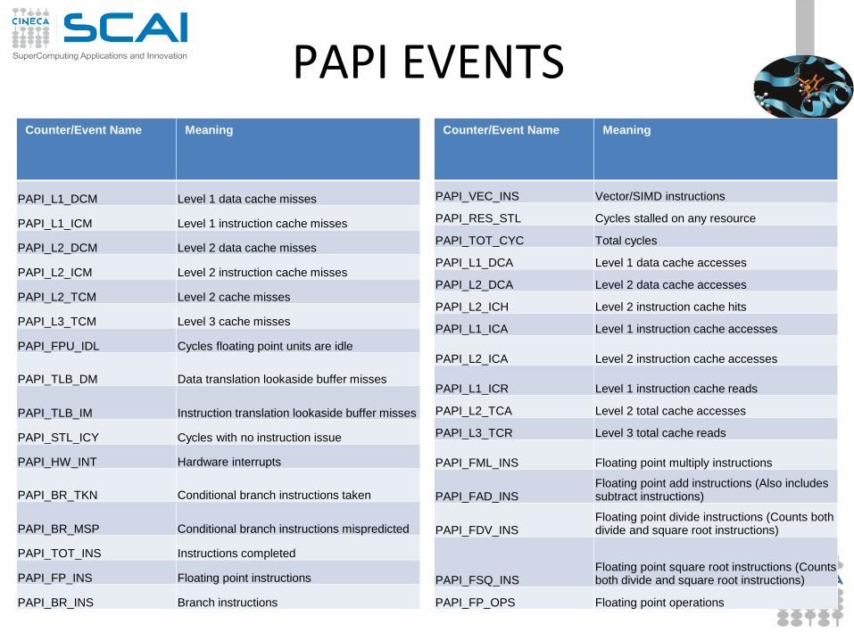
PAPI EVENTS Counter/Event Name Meaning

PAPI_L1_DCM Level 1 data cache misses

PAPI_L1_ICM Level 1 instruction cache misses

PAPI_L2_DCM Level 2 data cache misses

PAPI_L2_ICM Level 2 instruction cache misses

PAPI_L2_TCM Level 2 cache misses

PAPI_L3_TCM Level 3 cache misses

PAPI_FPU_IDL Cycles floating point units are idle

PAPI_TLB_DM Data translation lookaside buffer misses

PAPI_TLB_IM Instruction translation lookaside buffer misses

PAPI_STL_ICY Cycles with no instruction issue

PAPI_HW_INT Hardware interrupts

PAPI_BR_TKN Conditional branch instructions taken

PAPI_BR_MSP Conditional branch instructions mispredicted

PAPI_TOT_INS Instructions completed

PAPI_FP_INS Floating point instructions

PAPI_BR_INS Branch instructions

Counter/Event Name Meaning

PAPI_VEC_INS Vector/SIMD instructions

PAPI_RES_STL Cycles stalled on any resource

PAPI_TOT_CYC Total cycles

PAPI_L1_DCA Level 1 data cache accesses

PAPI_L2_DCA Level 2 data cache accesses

PAPI_L2_ICH Level 2 instruction cache hits

PAPI_L1_ICA Level 1 instruction cache accesses

PAPI_L2_ICA Level 2 instruction cache accesses

PAPI_L1_ICR Level 1 instruction cache reads

PAPI_L2_TCA Level 2 total cache accesses

PAPI_L3_TCR Level 3 total cache reads

PAPI_FML_INS Floating point multiply instructions

PAPI_FAD_INS Floating point add instructions (Also includes subtract instructions)

PAPI_FDV_INS Floating point divide instructions (Counts both divide and square root instructions)

PAPI_FSQ_INS Floating point square root instructions (Counts both divide and square root instructions)

PAPI_FP_OPS Floating point operations

#include <stdio.h>

#include <math.h>

#include <stdlib.h>

#include <time.h>

#define nn (2048)

double a[nn][nn], b[nn][nn], c[nn][nn]; /** matrici**/

int main()

{

int k, i, j, ii, jj;

float time1, time2, dub_time,somma;

/* initialize matrix */

time1 = clock();

for (j = 0; j < nn; j++)

{

for (i = 0; i < nn; i++)

{

a[j][i] = ((double)rand())/((double)RAND_MAX);

b[j][i] = ((double)rand())/((double)RAND_MAX);

c[j][i] = 0.0L;

}

}

time2 = clock();


printf("Tempo impiegato per inizializzare \n");

printf("Tempo -----------------> %f \n", dub_time);

time1 = clock();

for (i = 0; i < nn; i++)

for (k = 0; k < nn; k++)

for (j = 0; j < nn; j ++)

c[i][j] = c[i][j] + a[i][k]*b[k][j];

time2 = clock();


printf("===============================\n");}

Example

I Option

for (j = 0; j< nn; j++) for (k = 0; k < nn; k++) for (i = 0; i < nn; i ++) c[i][j] = c[i][j] + a[i][k]*b[k][j];

II Option

Example

Example

Tempi (s)

Dimension Opzione 1 Opzione 2

512 1.9 3.46

1024 10.42 19.45

2048 77.23 182.91

L1 Cache Missing


512 1.6938 E7 2.7585 E8

1024 1.3531 E8 2.2164 E9

2048 1.1339 E9 1.826 E10

MFlops


512 141.28 77.58

1024 206.09 110.41

2048 222.42 93.92

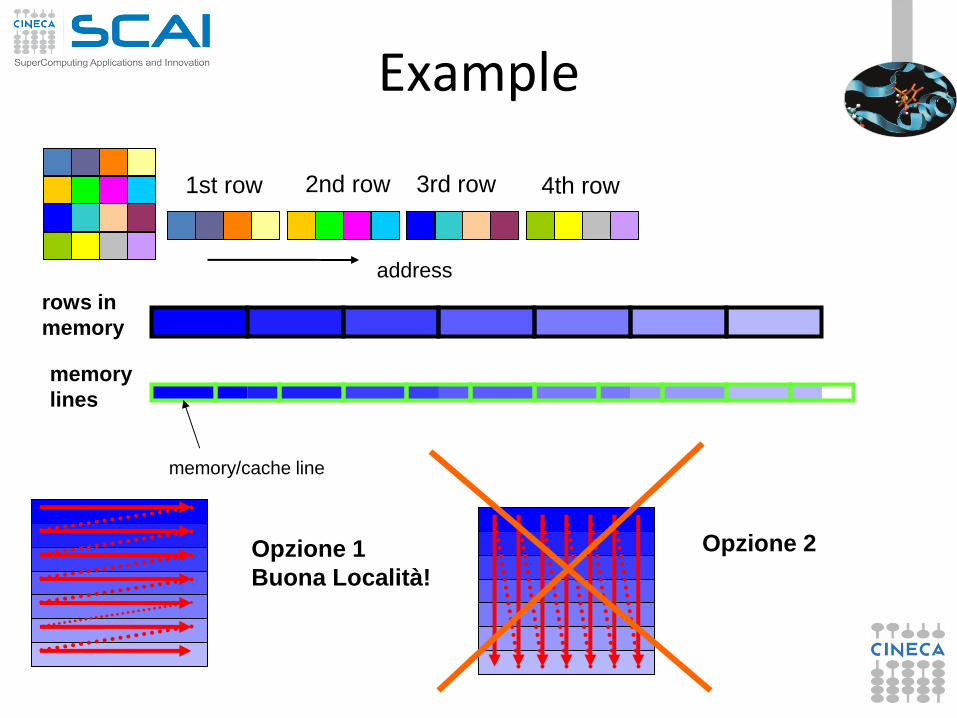
Example

1st row 2nd row 3rd row 4th row

address

rows in

memory

memory

lines

memory/cache line

Opzione 1

Buona Località!

Opzione 2

Documents

Profiling - Cineca · g++ -pg source code gfortran –pg source code – Run the executable to allow the generation of the files containing profiling information: o At the end of