Embed Size (px)
Citation preview
Prof. Aiken CS 294 Lecture 1 1
Program Analysis

Prof. Aiken CS 294 Lecture 1 2
The Purpose of this Course
• How are the following related?– Program analysis– Model checking (as applied to software)– Theorem proving (as applied to software)
• But program analysis itself has sub-disciplines . . .
Prof. Aiken CS 294 Lecture 1 3
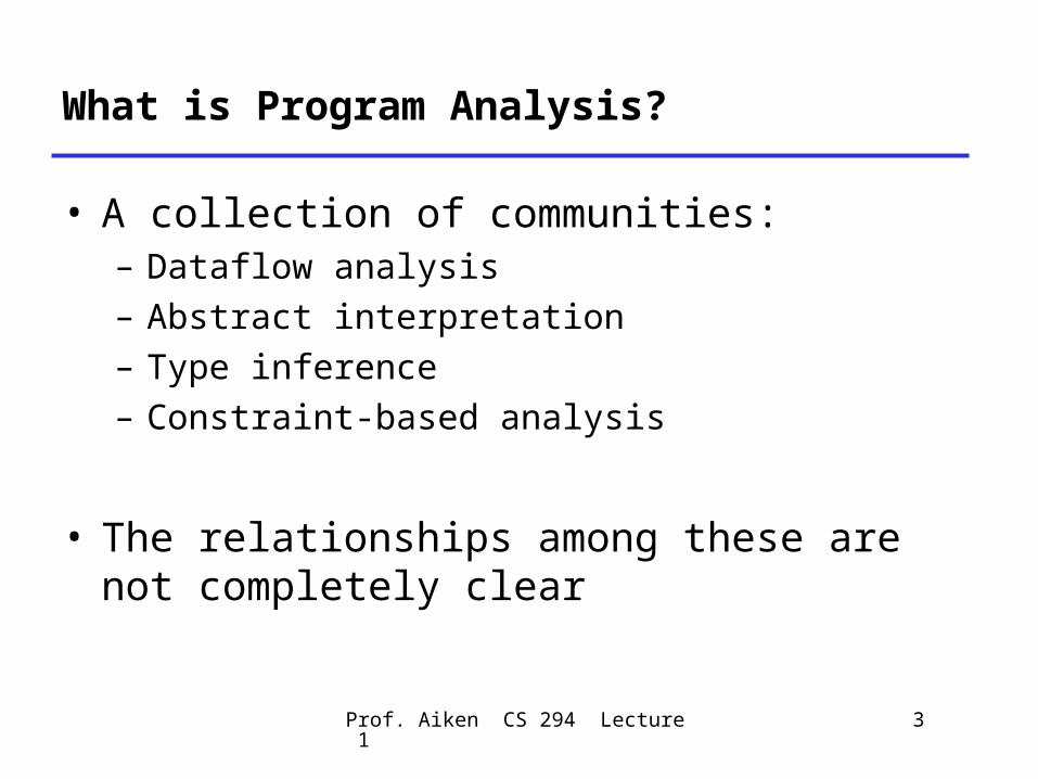
What is Program Analysis?
• A collection of communities:– Dataflow analysis– Abstract interpretation– Type inference– Constraint-based analysis
• The relationships among these are not completely clear

Prof. Aiken CS 294 Lecture 1 4
What is Program Analysis For?
• Historically: Optimizing compilers
• More recently:– Influencing language design– Finding bugs
Prof. Aiken CS 294 Lecture 1 5
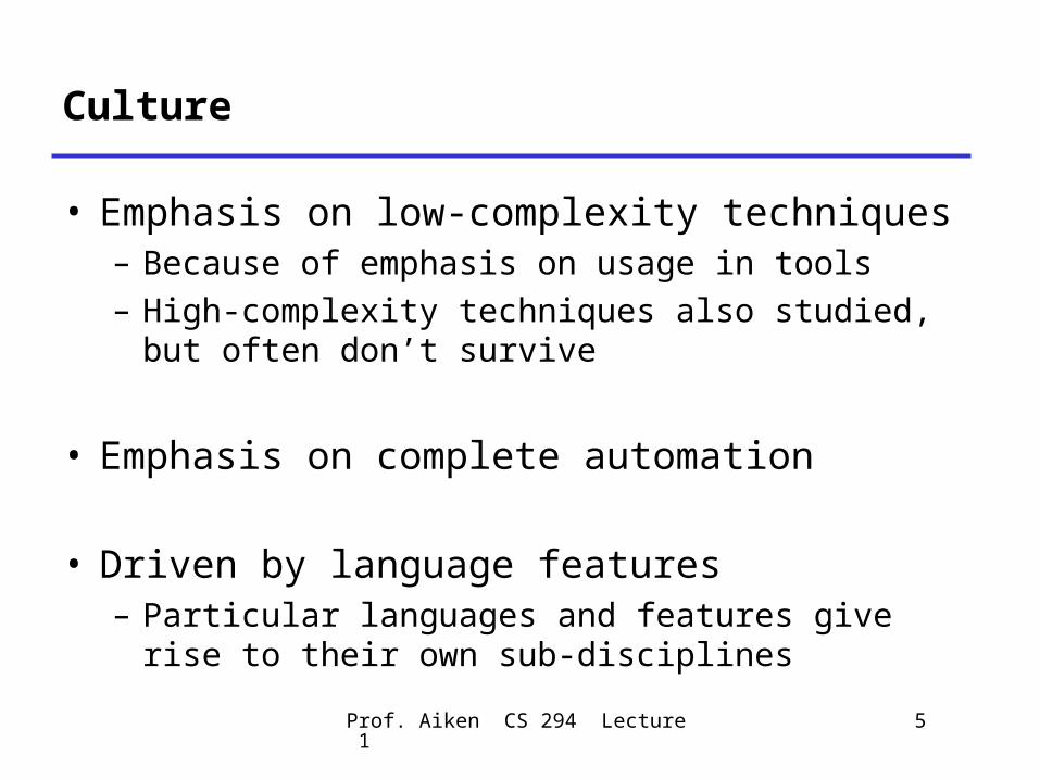
Culture
• Emphasis on low-complexity techniques– Because of emphasis on usage in tools– High-complexity techniques also studied, but
often don’t survive
• Emphasis on complete automation
• Driven by language features– Particular languages and features give rise to
their own sub-disciplines

Prof. Aiken CS 294 Lecture 1 6
Dataflow Analysis
Part 1

Prof. Aiken CS 294 Lecture 1 7
Control-Flow Graphs
x := a + b;y := a * b;while y > a + b {
a := a + 1; x := a + b}
if y > a + b
a := a + 1
x := a + b
y := a * b
x := a + b
Control-flow graphs are
state-transisition systems.

Prof. Aiken CS 294 Lecture 1 8
Notation
s is a statement succ(s) = { successor statements of s }pred(s) = { predecessor statements of s }write(s) = { variables written by s }read(s) = { variables read by s }
Note: In literature write = kill and read = gen
Prof. Aiken CS 294 Lecture 1 9
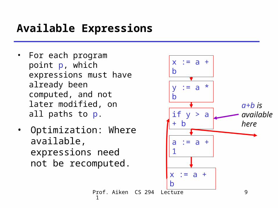
Available Expressions
• For each program point p, which expressions must have already been computed, and not later modified, on all paths to p.
if y > a + b
a := a + 1
x := a + b
y := a * b
x := a + b
• Optimization: Where available, expressions need not be recomputed.
a+b is available here

Prof. Aiken CS 294 Lecture 1 10
Dataflow Equations
( )
if ( )( ) ( ) otherwise
( ) ( ( ) | ( ) ( ) )
| if ( ) ( )
inout
s pred s
out in
pred sA s A s
A s A s a S write s V a
s write s read s

Prof. Aiken CS 294 Lecture 1 11
Example
if y > a + b
a := a + 1
x := a + b
y := a * b
x := a + b a+
b
a+b, a*b
a+b, a*b, y > a+b
a+b
a+b
a+b, y > a+b

Prof. Aiken CS 294 Lecture 1 12
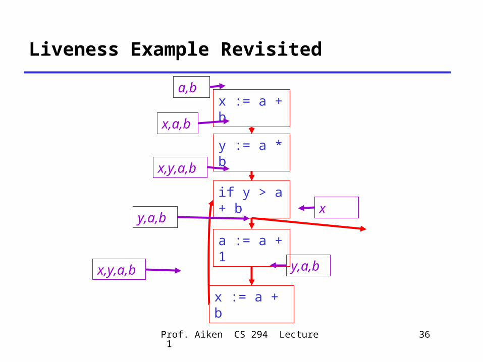
Liveness Analysis
• For each program point p, which of the variables defined at that point are used on some execution path?
if y > a + b
a := a + 1
x := a + b
y := a * b
x := a + b
• Optimization: If a variable is not live, no need to keep it in a register.
x is not live here
Prof. Aiken CS 294 Lecture 1 13
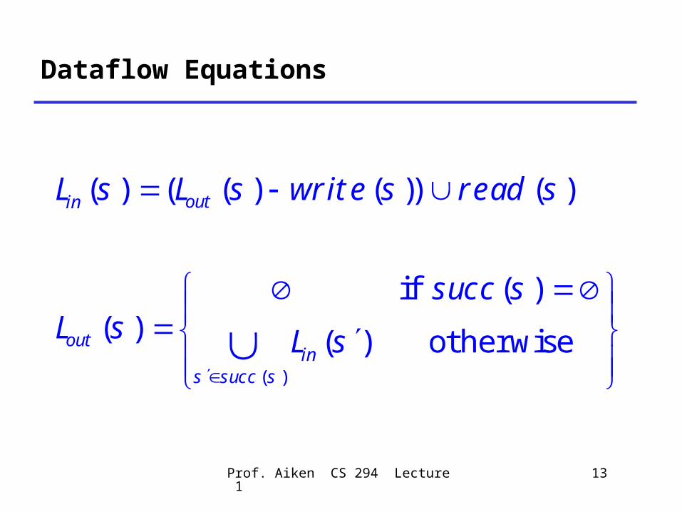
Dataflow Equations
( )
( ) ( ( ) ( )) ( )
if ( )( ) ( ) otherwise
outin
outin
s succ s
L s L s write s read s
succ sL s L s
Prof. Aiken CS 294 Lecture 1 14
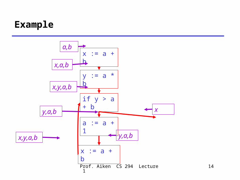
Example
if y > a + b
a := a + 1
x := a + b
y := a * b
x := a + b x,a,
b
x,y,a,b
y,a,b
y,a,bx,y,a,b
a,b
x

Prof. Aiken CS 294 Lecture 1 15
Available Expressions Again
( )
if ( )( ) ( ) otherwise
( ) ( ( ) | ( ) ( ) )
| ( ) ( )
inout
s pred s
out in
pred sA s A s
A s A s a S write s V a
s write s read s

Prof. Aiken CS 294 Lecture 1 16
Available Expressions: Schematic
( )
1 2
( ) ( )
( ) ( )
outins pred s
out in
A s A s
A s A s C C
Must analysis: property holds on all pathsForwards analysis: from inputs to outputs
Transfer function:

Prof. Aiken CS 294 Lecture 1 17
Live Variables Again
( )
( ) ( ( ) ( )) ( )
if ( )( ) ( ) otherwise
outin
outin
s succ s
L s L s write s read s
succ sL s L s
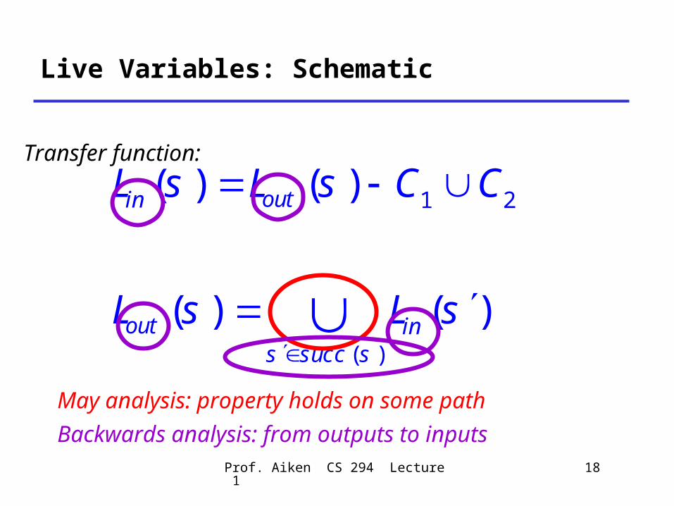
Prof. Aiken CS 294 Lecture 1 18
Live Variables: Schematic
1 2
( )
( ) ( )
( ) ( )
outin
out ins succ s
L s L s C C
L s L s
May analysis: property holds on some pathBackwards analysis: from outputs to inputs
Transfer function:

Prof. Aiken CS 294 Lecture 1 19
Very Busy Expressions
• An expression e is very busy at program point p if every path from p must evaluate e before any variable in e is redefined
• Optimization: hoisting expressions
• A must-analysis• A backwards analysis

Prof. Aiken CS 294 Lecture 1 20
Reaching Definitions
• For a program point p, which assignments made on paths reaching p have not been overwritten
• Connects definitions with uses (use-def chains)
• A may-anlaysis• A forwards analysis

Prof. Aiken CS 294 Lecture 1 21
One Cut at the Dataflow Design Space
May Must
Forwards Reaching definitions
Available expressions
Backwards Live variables Very busy expressions
Prof. Aiken CS 294 Lecture 1 22
The Literature
• Vast literature of dataflow analyses
• 90+% can be described by– Forwards or backwards– May or must
• Some oddballs, but not many– Bidirectional analyses
Prof. Aiken CS 294 Lecture 1 23
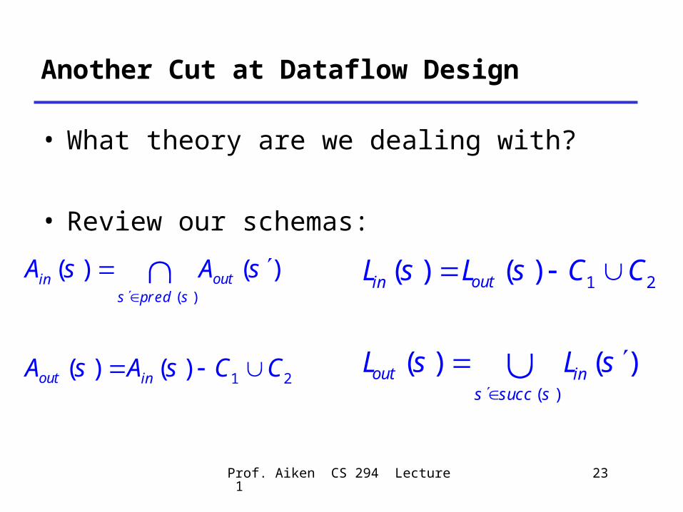
Another Cut at Dataflow Design
• What theory are we dealing with?
• Review our schemas:
( )
1 2
( ) ( )
( ) ( )
outins pred s
out in
A s A s
A s A s C C
1 2
( )
( ) ( )
( ) ( )
outin
out ins succ s
L s L s C C
L s L s

Prof. Aiken CS 294 Lecture 1 24
Essential Features
• Set variables Lin(s), Lout(S)
• Set operations: union, intersection– Restricted complement (- constant)
• Domain of atoms– E.g., variable names
• Equations with single variable on lhs

Prof. Aiken CS 294 Lecture 1 25
Dataflow Problems
• Many dataflow equations are described by the grammar:
• v is a variable• a is an atom• Note: More general than most problems . . .
; |
| | |
EQS v E EQS
E E E E E v a
Prof. Aiken CS 294 Lecture 1 26
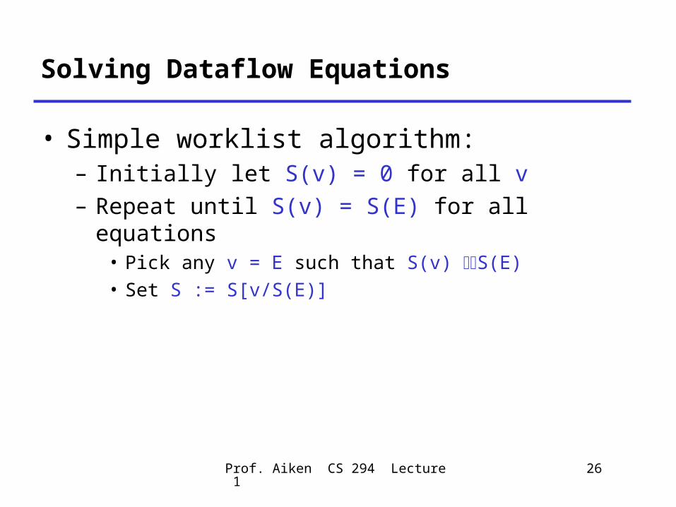
Solving Dataflow Equations
• Simple worklist algorithm:– Initially let S(v) = 0 for all v– Repeat until S(v) = S(E) for all equations
• Pick any v = E such that S(v) S(E)• Set S := S[v/S(E)]

Prof. Aiken CS 294 Lecture 1 27
Termination
• How do we know the algorithm terminates?
• Because– operations are monotonic– the domain is finite

Prof. Aiken CS 294 Lecture 1 28
Monotonicity
• Operation f is monotonic ifX Y f(x) f(y)
• We require that all operations be monotonic– Easy to check for the set operations – Easy to check for all transfer functions; recall:
1 2( ) ( )outinL s L s C C

Prof. Aiken CS 294 Lecture 1 29
Termination again
• To see the algorithm terminates– All variables start empty– Variables and rhs’s only increase with each
update • By induction on # of updates, using monotonicity
– Sets can only grow to a max finite size
• Together, these imply termination

Prof. Aiken CS 294 Lecture 1 30
The Rest of the Lecture
• Distributive Problems• Flow Sensitivity• Context Sensitivity
– Or interprocedural analysis
• What are the limits of dataflow analysis?

Prof. Aiken CS 294 Lecture 1 31
Distributive Dataflow Problems
• Monotonicity implies for a transfer function f:
• Distributive dataflow problems satisfy a stronger property:
f(x y) f(x) f(y)
f(x y) =f(x) f(y)

Prof. Aiken CS 294 Lecture 1 32
Distributivity Example
h
gf
k
k(h(f(0) g(0))) =
k(h(f(0)) h(g(0))) =
k(h(f(0))) k(h(g(0)))
The analysis of the graph is equivalent to combining the analysis of each path!

Prof. Aiken CS 294 Lecture 1 33
Meet Over All Paths
• If a dataflow problem is distributive, then the (least) solution of the dataflow equations is equivalent to the analyzing every path (including infinite ones) and combining the results
• Says joins cause no loss of information

Prof. Aiken CS 294 Lecture 1 34
Distributivity Again
• Obtaining the meet over all paths solution is a very powerful guarantee
• Says that dataflow analysis is really as good as you can do for a distributive problem.
• Alternatively, can be viewed as saying distributive problems are very easy indeed . . .

Prof. Aiken CS 294 Lecture 1 35
What Problems are Distributive?
• Many analyses of program structure are distributive– E.g., live variables, available expressions,
reaching definitions, very busy expressions– Properties of how the program computes
Prof. Aiken CS 294 Lecture 1 36
Liveness Example Revisited
if y > a + b
a := a + 1
x := a + b
y := a * b
x := a + b x,a,
b
x,y,a,b
y,a,b
y,a,bx,y,a,b
a,b
x

Prof. Aiken CS 294 Lecture 1 37
Constant Folding
• Ordering i< for any integer i• jk= if jk• Example transfer function:
• Consider
1 2 1 2( : ) [ ( ) ( ) ]
if , constantswhere
otherwise
C v e e v C e C e
a b a ba b
ú
( : )[ 1] ( : )[ 1]C z y y y C z y y y 7
( : )([ 1] [ 1])C z y y y y 7

Prof. Aiken CS 294 Lecture 1 38
What Problems are Not Distributive?
• Analyses of what the program computes– The output is (a constant, positive, …)
Prof. Aiken CS 294 Lecture 1 39
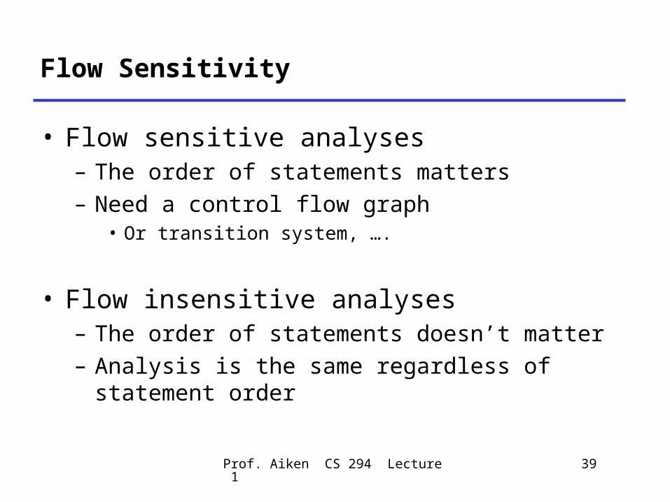
Flow Sensitivity
• Flow sensitive analyses– The order of statements matters– Need a control flow graph
• Or transition system, ….
• Flow insensitive analyses– The order of statements doesn’t matter– Analysis is the same regardless of statement
order

Prof. Aiken CS 294 Lecture 1 40
Example Flow Insensitive Analysis
• What variables does a program fragment modify?
1 2 1 2
( : )
( ; ) ( ) ( )
G x e x
G s s G s G s
• Note G(s1;s2) = G(s2;s1)

Prof. Aiken CS 294 Lecture 1 41
The Advantage
• Flow-sensitive analyses require a model of program state at each program point– E.g., liveness analysis, reaching definitions, …
• Flow-insensitive analyses require only a single global state– E.g., for G, the set of all variables modified

Prof. Aiken CS 294 Lecture 1 42
Notes on Flow Sensitivity
• Flow insensitive analyses seem weak, but:
• Flow sensitive analyses are hard to scale to very large programs– Additional cost: state size X # of program points
• Beyond 1000’s of lines of code, only flow insensitive analyses have been shown to scale

Prof. Aiken CS 294 Lecture 1 43
Context-Sensitive Analysis
• What about analyzing across procedure boundaries?
Def f(x){…}Def g(y){…f(a)…}Def h(z){…f(b)…}
• Goal: Specialize analysis of f to take advantage of• f is called with a by g• f is called with b by h

Prof. Aiken CS 294 Lecture 1 44
Control-Flow Graphs Again
• How do we extend control-flow graphs to procedures?
• Idea: Model procedure call f(a) by:– Edge from point before call to entry of f– Edge from exit(s) of f to point after call

Prof. Aiken CS 294 Lecture 1 45
Example
• Edges from – before f(a) to entry of f– Exit of f to after f(a)– Before f(b) to entry of f– Exit of f to after f(b)
f(x){…}
g(y){…f(a)…}
h(z){…f(b)…}

Prof. Aiken CS 294 Lecture 1 46
Example
• Edges from – before f(a) to entry of f– Exit of f to after f(a)– Before f(b) to entry of f– Exit of f to after f(b)
• Has the correct flows for g
f(x){…}
g(y){…f(a)…}
h(z){…f(b)…}

Prof. Aiken CS 294 Lecture 1 47
Example
• Edges from – before f(a) to entry of f– Exit of f to after f(a)– Before f(b) to entry of f– Exit of f to after f(b)
• Has the correct flows for h
f(x){…}
g(y){…f(a)…}
h(z){…f(b)…}

Prof. Aiken CS 294 Lecture 1 48
Example
• But also has flows we don’t want– One path captures a call
to g returning at h!
• So-called “infeasible paths”
f(x){…}
g(y){…f(a)…}
h(z){…f(b)…}

Prof. Aiken CS 294 Lecture 1 49
What to do?
• Must distinguish calls to f in different contexts
• Three techniques– Assumptions
• later
– Context-free reachability• Later
– Call strings• Today

Prof. Aiken CS 294 Lecture 1 50
Call Strings
• Observation: – At run time, different calls to f are distinguished
by the call stack
• Problem: – The stack is unbounded
• Idea:– Use the last k calls on the stack to distinguish
context– Represent a call by the name of the calling
procedure
Prof. Aiken CS 294 Lecture 1 51
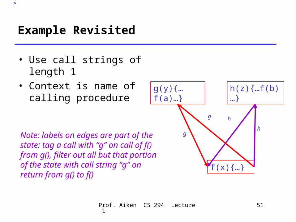
Example Revisited
• Use call strings of length 1
• Context is name of calling procedure
f(x){…}
g(y){…f(a)…}
h(z){…f(b)…}
g
g h
hNote: labels on edges are part of the state: tag a call with “g” on call of f() from g(), filter out all but that portion of the state with call string “g” on return from g() to f()

Prof. Aiken CS 294 Lecture 1 52
Experience with Call Strings
• Very expensive– Multiplies # of abstract values by (# of
procedures ** length of call string)– Hard to contemplate call strings > 1
• Fragile– Very sensitive to organization of procedures
• Well-studied, but not much used in practice

Prof. Aiken CS 294 Lecture 1 53
Review of Terminology
• Must vs. May• Forwards vs. Backwards• Flow-sensitive vs. Flow-insensitive• Context-sensitive vs. Context-insensitive• Distributive vs. non-Distributive

Prof. Aiken CS 294 Lecture 1 54
Where is Dataflow Analysis Useful?
• Best for flow-sensitive, context-insensitive, distributive problems on small pieces of code– E.g., the examples we’ve seen and many others
• Extremely efficient algorithms are known– Use different representation than control-flow
graph, but not fundamentally different– More on this in a minute . . .

Prof. Aiken CS 294 Lecture 1 55
Where is Dataflow Analysis Weak?
• Lots of places

Prof. Aiken CS 294 Lecture 1 56
Data Structures
• Not good at analyzing data structures
• Works well for atomic values– Labels, constants, variable names
• Not easily extended to arrays, lists, trees, etc.– Work on shape analysis
Prof. Aiken CS 294 Lecture 1 57
The Heap
• Good at analyzing flow of values in local variables
• No notion of the heap in traditional dataflow applications
• In general, very hard to model anonymous values accurately– Aliasing– The “strong update” problem

Prof. Aiken CS 294 Lecture 1 58
Context Sensitivity
• Standard dataflow techniques for handling context sensitivity don’t scale well
• Brittle under common program edits
• E.g., call strings

Prof. Aiken CS 294 Lecture 1 59
Flow Sensitivity (Beyond Procedures)
• Flow sensitive analyses are standard for analyzing single procedures
• Not used (or not aware of uses) for whole programs– Too expensive
Prof. Aiken CS 294 Lecture 1 60
The Call Graph
• Dataflow analysis requires a call graph– Or something close
• Inadequate for higher-order programs– First class functions– Object-oriented languages with dynamic dispatch
• Call-graph hinders algorithmic efficiency– Desire to keep executable specification is limiting

Prof. Aiken CS 294 Lecture 1 61
Forwards vs. Backwards
• Restriction to forwards/backwards reachability– Very constraining– Many important problems not easy to fit into
this mold

Prof. Aiken CS 294 Lecture 1 62
Next Time: Abstract Interpretation
• Theory– Lots
• Examples– Lots
• Focus on contrast with traditional dataflow analysis