BROOKINGS DISCUSSION PAPERS IN INTERNATIONAL ECONOMICS

No. 132

PRODUCTIVITY GROWTH: DISCUSSION AND TWELVE SECTOR SURVEY

Philip Bagnoli

April 1997

Philip Bagnoli is an economist with the EconomicStudies and Policy Analysis Division of the Departmentof Finance in Ottawa. This work was undertaken whilehe was a resident Research Associate in the EconomicStudies Program of the Brookings Institution. Thisproject has received financial support from the U.S.Environmental Protection Agency through CooperativeAgreement CR-818579-01-0 and from the National ScienceFoundation through grant SBR-9321010. The authorthanks Warwick McKibbin and Peter Wilcoxen forcomments on earlier drafts and Barry Bosworth andCharles Schultze for helpful discussions. The viewsexpressed are the author’s and should not beinterpreted as reflecting the views of the Departmentof Finance, the trustees, officers or other staff ofthe Brookings Institution, the EnvironmentalProtection Agency or the National Science Foundation.

Brookings Discussion Papers in International Economicsare circulated to stimulate discussion and criticalcomment. They have not been exposed to the regularBrookings prepublication review and editorial process. References in publications to this material, otherthan acknowledgment by a writer who has had access toit, should be cleared with the author.

PRODUCTIVITY GROWTH:DISCUSSION AND TWELVE SECTOR SURVEY

ABSTRACT

This paper surveys productivity growth at a sectoral level for the United States and othercountries. We begin with a discussion of the definition and measurement of productivity growth followedby a review of empirical work undertaken in its measurement.

We then take a close look at factors influencing productivity growth in twelve sectors: electricutilities; gas utilities; petroleum refining; coal mining; crude oil and gas extraction; other mining;agriculture, fishing and hunting; forestry and wood products; durable manufacturing; non-durablemanufacturing; transportation; and services. The paper reports differential productivity growth rates forthese industries for the United States and for subsets of these industries for other countries.

Philip BagnoliDepartment of Finance, Ottawa, ON.The Brookings Institution, Washington, DC.

1

I. Introduction

Almost four decades have elapsed since Solow (1957) argued that productivity growth was a

major factor in the growth of national output. Since that time much analysis has been conducted into the

sources of productivity growth and into the factors that affect its magnitude. Subsequent studies have

enhanced his original 2-factor model to account for a larger number of inputs and a change in the quality

of those inputs: the Solow residual is now much smaller than originally calculated -- though its economic

importance remains considerable. Some of the more careful and detailed of the subsequent studies (e.g.

Denison [1974], Maddison [1987] or Jorgenson, Gollop and Fraumeni [1987]) suggest that the remaining

residual accounts for about one quarter of growth for the period beginning in the late 1940's. At least one

study which tries to account for the input of students' time into building human capital (Jorgenson and

Fraumeni [1992]) puts the residual growth at about one sixth of total growth during that period.

Diewert (1992) undertook a critical review of the metrics used in gauging productivity growth.

He provides strong theoretical arguments for well known criticisms of some of the traditional techniques

of measuring productivity growth and suggests that index number theory might be the only foundation for

providing reasonable measures of productivity growth.

This paper will outline these as well as other major issues that must be addressed in productivity

analysis and summarizes the results of previous work done in this area. Our intention is to provide an

introduction to the current state of research in productivity analysis (future work will then take this basis

as a point of departure). We begin in the next section (II) with a simple illustration of productivity

growth and its measurement followed by a discussion of conceptual and empirical issues in attempting to

measure productivity growth. The following section (III) will provide a literature review and detail

elements of some of the important work that has been done. Section IV then surveys historical factors in

1The disaggregation corresponds to the sectors of the GCUBED model, see McKibbin andWilcoxen (1995).

2The measure given by equation (2) has become known as the Solow residual. An alternativeview of the residual is given by Real Business Cycle theorists who treat it as a random variable and thusargue that productivity shocks are the sources of fluctuations in economic activity (see Prescott [1987]).

2

productivity growth in a 12 sector disaggregation1, followed by the final section (V) which concludes by

illustrating the implications of historical productivity growth on the twelve sectors.

II. Background

Traditionally, three basic approaches have been used in measuring total factor productivity (TFP)

growth. These are based on: (1) production functions; (2) cost functions; and (3) inference through index

numbers. The approach used by Solow (1957) to argue that technological progress was an important

component of economic growth was based on the first method and can be illustrated with the following

production function:

(1)Where: Y is output,

KP is physical capital,KH is human capital,M is materials.

TFP growth occurs when changes in output Y cannot be attributed to changes in one of the three inputs2,

i.e.:

(2)

At the level of the aggregate economy when output is aggregated to one good the materials input is very

small and is generally ignored: it is dominated by the value-added attributable to physical and human

capital in the final product; moreover, the total volume of material inputs does not show large changes

3

over time (at a sectoral level, however, materials are the dominant input for most industries).

Equation (2), however, has drawbacks as a measure of productivity gains. It is sensitive to both

the measurement of aggregate inputs as well as the correct parameterization of the production function.

Take, for example, a Cobb-Douglas function; if Gross Domestic Product (GDP) is the output measure

then we have,

(3)

Increases in Bt measure TFP gains, while $k and $l are parameters. The measurement of TFP gains is

clearly sensitive to the accuracy of measured changes in physical and human capital and, as well, the

accuracy with which the parameters $k and $l have been measured. The problem of measuring $k and $l

can be overcome with the aid of the following assumptions:

(1) competitive markets,(2) constant returns to scale,(3) no externalities which create a wedge between social and private marginal costs.

These assumptions allow us to use cost shares (i.e. deflated nominal factor returns) in place of the Cobb-

Douglas parameters so that we have:

(4)

where sk and sl are the capital and labor cost shares, respectively and and are physical and human

capital, respectively.

This equation is no longer parametric, it holds for any form of the production function that

satisfies the three assumptions given above. It is, therefore, a powerful tool in productivity measurement

which has come into widespread use. As we shall see, however, there are still important caveats that must

be acknowedged. The remainder of this section will first discuss some additional conceptual issues in

measuring productivity growth followed by more specific discussions of data measurement issues,

4

international productivity comparisons, and the use of cost functions and index numbers to measure

productivity growth.

Many authors specify the production function with a measure of labor input (e.g. number of hours

worked) and then make adjustments for changes in the quality of labor so as to get a measure of human

capital (see Denison [1962]). Some authors, however, do not (e.g. Glaser [1992]). This inconsistency

stems from differences in the objectives of researchers: authors who use the correction are attempting to

carefully account for changes in output that are linked to measurable changes in inputs (growth

accounting), those who do not are measuring a rough approximation of welfare by looking at changes in

the amount of output that can be obtained for a given unit of labor input -- i.e. how much material goods

do we get for our efforts.

Inherent in the distinction just made is the notion that, for growth accounting, human and physical

capital must be treated symmetrically. That is, human capital is built through investment -- requiring the

postponement of consumption -- in acquiring skills much the same way physical capital is built by

accumulated investment in physical equipment. Both types of capital are subject to depreciation, with

human capital depreciation occurs slowly since the stock is reduced only through the withdrawl of labour

services. It is this distinction that lead Jorgenson and Fraumeni (1992) conclude that residual growth is

only one sixth of output growth in the post-war period when we account for student’s time in building

human capital.

Pushing this argument further leads us to acknowledged that output growth which is the result of

research and development (R&D) -- leading to improvements in physical and human capital -- is in fact a

return to the investment made in R&D. This can be distinguished from output growth that occurs through

the pure synergy of labor working with capital and producing additional output with no investment in

acquiring new knowledge. A growth accounting effort, therefore, that fully accounted for changes in

inputs would have to account for returns to R&D. This treatment of R&D as a factor of production leads

3Denison (1962) provides some justification for making the assumptions previously outlined andconcludes that these assumptions are tenable for the aggregate economy but are less tenable at high levelsof disaggregation

5

to the observation that firms invest in it until its marginal cost equals the value of its contribution to

revenues. The residual, therefore, after accounting for the cost of R&D would imply that TFP measured

primarily gains in output that were unaccounted for elsewhere; that is, it would measure quasi-rents

originating in a capital/labour synergy or in excess returns to improvements in production technologies.

It should be emphasized that equation (4) is highly aggregated. To write such an equation for the

aggregate economy requires not only the three assumptions outlined earlier3 (which made equation (4)

operational) but also other restrictive assumptions which are embodied in an aggregate production

function. For example, since the economy produces many goods which are aggregated into a total

measure of output, the aggregate production function will have many underlying sectoral production

functions which must be identical replicates of the aggregate. It is not sufficient that the sectoral capital

shares be equal on average to the aggregate capital share, they must be identical to the aggregate (recall

that logarithms are not additive, i.e. log {a+b}…log{a}+log{b} ).

Turning to the measurement of Bt (as specified in equation 4), we begin by highlighting that, as

was pointed out by Nordhaus (1987), economists have made considerable effort in measuring the rate of

productivity growth but little has been done to explain the determinants of that growth rate. Models of

endogenous growth (e.g. Romer [1990]) elucidate the process which creates productivity growth but do

not provide explanations as to the magnitude of that growth rate; and, by implication, do not explain

changes in productivity growth rates. Recent history has shown periods of high productivity growth

where its average rate was .8% of GDP per year for more than two decades followed by a period of

virtually no productivity growth at all. A critical transition from high productivity growth to low growth

4Krugman (1994) suggests that a technological catchup at the end of the war was responsible forthe exceptional growth rate and was largely exhausted by late 1960's. Jorgenson (1984) suggests itsprinciple cause was the oil price shock.

6

seems to have occurred during the late 1960's to early 1970's (see Nordhaus, [1972] and Denison [1979]).

While many anecdotal as well as empirical arguments have been suggested regarding the sources of that

change, none has been found to be convincing4.

a. Data Problems and the Measurement of a Residual

As was mentioned earlier, current estimates of TFP growth are smaller than they initially were

but they remain economically very significant. The basis on which these estimates are made, however,

remains the subject of some discussion among researchers -- Denison (1962) and Christensen and

Jorgenson (1969) made important contributions in measuring labor and capital inputs but there remain

limitations created by the lack of adequate data. Consider the level of detail necessary to adequately

measure the sources of labor productivity: the amount of human capital being used for specific tasks

should be known so as to control for changes in the quantity of human capital being applied to the task.

Changes in human capital include changes in the level of training and education of labor and their costs

should be excluded from the TFP measurement because they represent an investment: any additional

output resulting from that investment cannot be considered a TFP gain if it just covers the cost of the

investment.

In the past, changes in human capital have been approximated by changes in the number of years

of formal schooling of the population. While this measure may in fact be correlated with the quality of

the labor input the correlation may be imperfect. Indeed, Mulligan and Sala-i-Martin (1995) make this

argument and show that, using their “optimal” estimates of human capital, the 1980's were a period where

the average stock of human capital and the average number of years of formal education actually moved

in different directions -- thus giving opposing answers to the question of whether increased dispersion in

5It has been suggested that formal schooling serves as a screening mechanism to identifyindividuals with specialized characteristics who are then channeled into professions by a self-selectionprocess. If this is the case then formal education will be a good indicator primarily of how the screeningprocess works and only secondarily of the quality of labor.

7

human capital may have contributed to the increased dispersion in incomes5.

The foregoing observations are also applicable to changes in the quality of the capital input.

Measurement of changes in capital should account for technological improvements that were being

embodied in new capital stocks (see Solow [1960]) since the additional output from the technological

improvement is a return to the investment made in obtaining the technology (R&D). Furthermore, to get

a true measure of the sources of TFP growth this data would have to be available for a complete business

cycle to eliminate cyclical factors (e.g. labor hoarding which would distort labor input measurements).

Another source of limitations created by the data is that output cannot always be measured in a

cost efficient manner and must therefore be estimated. This problem is most common in the service

sectors, especially those relating to financial services. Since the output of many service sector industries

varies from firm to firm and is not always priced directly (e.g. most bank transactions are not individually

priced but are paid for through the interest spread on loans and deposits), gathering exact data that could

be used for TFP measurement is not feasible. In these industries output is sometimes measured as the

value of the inputs -- often it is measured simply as the value of the labor input. The working premise is

that productivity improvements accrue to the inputs in the form of higher returns. As a result, in the

banking sector productivity improvements would, by definition, be non-existent. More generally,

however, in industries where input markets are competitive while output markets are not this technique

will fail to measure TFP changes because the gains will accrue to the owners of the firm (which can still

be measured but only if the analysis is sufficiently detailed). Output markets may not be competitive in

times technological change where new technologies create quasi-rents for innovating firms (some argue

that the economy is dominated by monopolistic competition, see Akerlof, Dickens and Perry, 1996, and

the references therein). Furthermore, since the output price is often not being measured correctly (see

8

CBO [1995] for a discussion of problems with the Consumer Price Index), changes that go primarily to

consumers in increased consumer surplus are also not being captured; for example, when neutral

productivity improvements allow an industry to produce more output with the same inputs but demand

elasticity is near unity there may be little change in revenues in spite of an increase in output. If the

output price index is not carefully measured the changes could be completely missed in productivity

analysis even though the industry would have undergone significant changes in output.

The implication of the foregoing remarks is that the elements that go into the production function

for estimating TFP growth may have considerable error in their measurement. As was outlined earlier,

any errors in measuring inputs poses problems for the measurement of TFP growth.

b. Non-stationary Inputs and Outputs

As is discussed in Feenstra and Markusen (1994) and Diewert (1992) new inputs and outputs not

only cause mis-measurement of productivity growth but also raise questions about the usefulness of the

exercise. The nature of the problem is easily understood by considering equation (2) and asking what

would be the value of a measure between two time periods where the human capital could be measured

consistently over time but the units of measure of capital and output had changed. They would, in

essence, be two different economies which can only be compared by looking at the level of welfare

attained per unit of human capital.

Perhaps the best means of dealing with this problem is to emphasize short term measures of TFP

growth and make less use of long term TFP. Unfortunately, short-term TFP calculations have their own

problems in dealing with business cycle issues.

9

Cross-Country Studies

International comparisons of TFP growth are particularly difficult because of the onerous data

requirements. We have argued that the data requirements for analysis of TFP growth can be heavy when

one is looking for the source of TFP growth in an economy that produces many goods and services which

change over time. To conduct the same study across economies further requires that the data be

consistently defined across a number of national sources. For the system of national accounts (SNA) a

common definition exists and is adhered to by most of the world's national statistical agencies. However,

for other data collected this is not always true; for example, most OECD countries report employment

data which cannot be directly compared.

Another source of difficulties that arises in making international comparisons is that of selecting

units of measurement. Since different economies tend to produce a different mix of goods and services --

which change over time -- it is not possible to simply compare the number of units being produced across

countries. Fortunately, the apparatus necessary to compare national outputs has been developed

considerably by a number of international organizations starting from the initial work of Heston and

Summers (1980). Both the OECD and the IMF now pay special attention to obtaining indices of national

output through the use of purchasing power parity (PPP) measurements (the OECD has a somewhat

longer tradition of calculating PPP's). In spite of considerable effort, however, these numbers still

provide measurements which fail to inspire confidence. The OECD and IMF indices often differ

considerably and the OECD numbers tend to vary by uncomfortably large amounts across base years.

A third problem in making international comparisons is with the periods chosen. As was

mentioned earlier, it is important to avoid periods where the business cycle might distort the

measurements of TFP growth. This problem becomes even more difficult to overcome when many

countries are involved because it is very unlikely that a starting and end point can be found where all

countries will be at the same point in the business cycle. While this problem cannot be completely

10

eliminated its effect can be minimized by choosing as long a period as possible, thereby distributing the

measurement error over many years.

Index Numbers and Cost Functions

The discussion thus far took the production function as its point of departure, it then quickly

moved to more restrictive but non-parametric form based on cost shares. The change was necessary

because the production function is not econometrically identified in its unresticted form. For the

parameters to be identified would require that stringent a priori restrictions be imposed (for a broader

discussion see Diewert [1992]). As was mentioned earlier, however, there are alternatives in measuring

TFP growth. A less restrictive strategy involves the use of cost functions. By assuming cost minimizing

behavior and using Shephard’s Lemma the number of parameters that must be estimated while retaining

generality in the functional form can be reduced. The remaining problem with the cost function technique

(which is also a problem with production function techniques) is that many parameterizations of the cost

functions are possible, all of which are valid but each of which is likely to give different rates of TFP

growth. Since little formal criteria exists for choosing among the alternatives, in general researchers

choose one that best suits the task at hand. In many cases, however, this leads to measurements which

can not be directly compared to other studies.

The most promising technique for measuring TFP growth is through the use of index numbers

(Diewert [1979]). Index numbers are better suited to measuring TFP growth for two related reasons:

first, most indices have a commonality in their construction so there is less contradiction with the

measured values than there is with production or cost function based measurements. Second, indices do

not force a particular structure on the data. This latter point is important but it may also be considered a

drawback of index numbers. For example, when one is trying to account for the sources of growth, an

index number provides little guidance as to how the allocation of increases in output should be divided

11

Table I(1) structural change(2) convergence to technology leader(3) foreign trade effects(4) economies of scale(5) energy price shocks(6) natural resource discovery(7) costs of government regulation and crime(8) labor hoarding(9) capacity utilization effects

Source: Maddison (1987)

among the inputs.

III. Literature Review

a. aggregate analysis

In spite of the problems just discussed a

number of studies have undertaken a comparison of

productivity growth on an international scale. One of

the earliest studies was Denison (1967) where sources of growth in the United States and nine European

countries were compared for the period 1950 to 1962. Denison essentially applies on an international

scale the techniques he developed in earlier work (e.g. Denison [1962]) to analyze the US economy.

Similar to his earlier work -- and to Solow (1957) -- the results he obtains suggest that "Advances of

knowledge" was a major contributor to growth in the US and the European countries in a disaggregation

that included nineteen different factors. In that work, however, Denison argues that changes in Advances

of knowledge should only be measured for the most advanced economy. His reasoning is that other

countries which are behind the technology leader will in general be catching up to the best practice of the

leader, therefore, much of the residual that would be measured as Advances of knowledge in those

countries would simply reflect implementation of existing best practice -- in other words, “adoption of

knowledge”.

Maddison (1987) reviews comparative growth studies and outlines the essentials of growth

accounting with an illustrative long term analysis of growth in four European countries, Japan and the

United States. He divides inputs into three categories (Capital, Labor and Other Factors) and then

demonstrates how successive refinements to quality change in those inputs reduces the measured to 25%

of actual growth. residual . Table I lists his Other Factors. As is obvious from the table, some of the

factors that might be associated with productivity growth are included as part of that input. The residual

12

that is measured, therefore, is more a statement of unmeasurable effects than it is a measure of

productivity change. Moreover, what is uncomfortably clear in his work is that TFP growth that is

measured as a residual is critically dependent of the measurement and definition of the inputs. Maddison

concludes that the full model can explain, on average, approximately 75% of the growth in Europe, Japan

and the U.S. that occurred between 1913 and 1950, leaving a significant role for the residual “TFP”

growth. He points out, however, that the ability of the model to explain growth varies across countries

and across time periods.

Additional studies in productivity growth are found in Table II where we present a summary of

GDP growth rates and the measured TFP growth for a number of major countries and regions. With a

few notable exceptions, we find that there is surprising agreement among results. This occurs in spite of

our earlier comments regarding the techniques and objectives of researchers.

Recently, new databases have been developed in the Penn World Tables and for projects at the

World Bank which -- when combined with recent improvements in the International Labor Organization

(ILO) databases -- make more rigorous analysis possible beyond the conventional few industrialized

countries. Bosworth, Collins and Chen (1995) use the data on human and physical capital to look at the

extent to which growth outside the industrialized regions is in factor deepening rather than productivity

growth. They tentatively conclude that in most cases it is the mobilization of resources that accounts for

growth. In an interesting application of computable general equilibrium modeling Chenery, Robinson

and Syrquin (1986) examine the importance of various policy and institutional settings for the

development process. Part of their survey of empirical work is presented in Table II.

Gordon (1995) attempts to examine a tradeoff between TFP growth and unemployment in the

Group of Seven countries. He develops a consistent database of hours worked by pooling together data

from various sources. Some of his empirical results are also found in Table II.

Table II: Studies of Economy-Wide Growth in a Range of Countries

Maddison (1989) Gordon (1995) (a) Bosworth/Collins/Chen (1995) GDP TFP Cont. Cont. Output TFP Cont. Cont. GDP TFP Cont. Cont.Country Period Growth Growth Capital Labor Period Growth Growth Capital Labor Period Growth Growth Capital Labor

U.S. 1950-73 3.65 1.49 1.02 1.14 * 1960-73 3.12 1.35 0.95 0.82 * 1960-70 3.61 0.90 0.98 1.73 1973-84 2.42 0.25 0.84 1.33 * 1973-79 2.69 -0.14 1.31 1.52 * 1970-80 2.96 -0.50 0.97 2.49

1979-92 2.29 0.38 1.17 0.74 * 1980-86 2.71 0.90 0.78 1.03 1986-92 2.24 0.60 0.77 0.87

Japan 1950-73 9.29 5.47 2.37 1.45 * 1960-73 7.72 --- --- * 1960-70 10.12 5.00 4.17 0.95 1973-84 3.72 1.99 1.00 0.73 * 1973-79 3.29 1.29 1.86 0.14 * 1970-80 4.52 0.50 2.78 1.24

1979-92 3.98 1.63 1.83 0.52 * 1980-86 3.66 1.10 1.52 1.04 1986-92 4.07 1.00 1.74 1.33

France 1950-73 5.13 3.69 1.07 0.37 * 1960-73 5.62 3.64 1.49 0.49 * 1960-70 5.64 2.50 2.32 0.82 1973-84 2.32 1.47 1.20 -0.35 * 1973-79 3.84 2.39 1.52 -0.07 * 1970-80 3.66 0.80 1.76 1.10

1979-92 2.59 1.57 0.99 0.03 * 1980-86 2.42 0.50 1.09 0.84 1986-92 2.61 0.80 0.95 0.86

Germany 1950-73 5.92 4.14 1.59 0.19 * 1960-73 5.27 3.43 1.88 -0.04 * 1960-70 4.34 2.20 1.81 0.33 1973-84 1.72 1.48 1.01 -0.77 * 1973-79 3.95 2.69 1.55 -0.29 * 1970-80 2.93 1.20 1.23 0.50

1979-92 4.40 1.44 1.57 1.39 * 1980-86 2.11 0.60 0.91 0.60 1986-92 6.64 1.40 1.75 3.49

U.K. 1950-73 3.02 1.98 0.98 0.06 * 1960-73 3.36 2.32 1.15 -0.12 * 1960-70 2.82 1.10 1.57 0.15 1973-84 1.10 1.19 0.76 -0.85 * 1973-79 2.43 1.16 1.11 0.16 * 1970-80 2.21 0.20 1.15 0.86

1979-92 1.51 1.22 0.13 0.17 * 1980-86 3.41 1.60 0.91 0.89 1986-92 1.30 0.00 0.89 0.41

Canada 1960-73 3.02 2.30 0.72 * 1960-70 4.73 1.60 1.16 1.97 1973-79 1.27 0.36 0.91 * 1970-80 4.70 0.20 1.46 3.04 1979-92 1.41 -0.04 1.45 * 1980-86 3.31 0.60 1.38 1.33

1986-92 2.02 -0.50 1.50 1.02 Italy 1960-73 6.71 5.56 1.15 * 1960-70 5.72 3.60 1.99 0.13

1973-79 1.99 2.63 -0.64 * 1970-80 3.89 1.70 1.34 0.85 1979-92 1.90 1.71 0.19 * 1980-86 2.31 0.20 0.97 1.14

1986-92 2.39 0.70 0.88 0.81 Australia 1960-70 5.14 1.10 1.77 2.27

1970-80 3.64 0.80 1.48 1.36 1980-86 3.24 0.50 1.11 1.63 1986-92 3.10 0.60 1.00 1.50

China 1950-73 5.84 0.49 2.74 2.61 1960-70 3.60 1.30 0.76 1.54 1973-84 6.85 2.10 2.35 2.40 1970-80 4.91 0.80 2.58 1.53

1980-86 8.49 4.00 3.06 1.44 1986-92 7.69 2.50 3.70 1.50

Korea 1950-73 7.49 2.84 1.84 2.81 * 1960-70 6.83 0.60 4.19 2.04 1973-84 7.38 1.42 3.03 2.93 * 1970-80 7.64 0.80 5.20 1.64

1980-86 7.49 2.50 3.41 1.57 1986-92 7.59 1.90 4.29 1.39

Taiwan 1950-73 9.32 3.51 2.32 3.49 1960-70 9.63 1.40 5.75 2.48 1973-84 7.63 1.23 2.83 3.57 1970-80 8.06 1.10 4.88 2.07

1980-86 4.50 1.80 2.10 0.60 1986-92 5.90 2.50 2.80 0.60

India 1950-73 3.69 -0.05 1.84 1.90 1960-70 4.09 0.50 2.28 1.31 1973-84 4.29 0.50 1.37 2.42 1970-80 3.57 -0.20 2.01 1.76

1980-86 5.35 1.80 1.96 1.59 1986-92 5.35 1.50 2.22 1.63

Argentina 1950-73 3.78 1.38 1.05 1.35 1960-70 4.02 1.10 1.89 1.03 1973-84 0.69 -1.58 0.62 1.65 1970-80 3.35 -0.10 2.16 1.29

1980-86 -0.59 -2.00 0.37 1.05 1986-92 1.85 1.10 -0.20 0.95

Brazil 1950-73 6.75 2.13 2.15 2.47 1960-70 5.11 1.60 2.10 1.41 1973-84 4.33 -1.97 2.90 3.40 1970-80 7.24 2.40 3.34 1.51

1980-86 2.19 -1.10 1.58 1.72 1986-92 -0.09 -2.60 1.02 1.48

Chile 1950-73 3.67 1.60 1.06 1.01 1960-70 4.16 1.40 1.62 1.13 1973-84 1.24 -0.92 0.58 1.58 1970-80 1.67 0.00 0.43 1.24

1980-86 -0.22 -1.90 0.37 1.31 1986-92 6.75 3.80 1.66 1.29

Mexico 1950-73 6.38 1.91 2.06 2.41 1960-70 6.34 1.70 2.96 1.68 1973-84 4.55 -0.64 2.28 2.91 1970-80 4.93 0.40 2.73 1.80

1980-86 -0.07 -3.50 1.55 1.88 1986-92 1.99 -0.90 0.82 2.07

USSR 1950-73 5.05 0.50 2.76 1.79 *1973-84 2.16 -1.40 2.00 1.56 *

Notes: CCJ: Christensen, Cummings and Jorgenson (1995),Ah: Aluwalia (1985), Y: Young (1994).References for E: Elias (1978), El: Elias (1990), and D: Dougherty (1991) are found in Barro and Sala-i-Martin (1995)(a) Gordon reports Nonfarm Private Business Sector. For Italy and Canada Output/Hour is reported.* Labor is measured in hours workedGrowth in Labor Force is proxied by growth in population in Chenery/Robinson/Syrquin (1995) and Barro/Sala-i-Martin (1995) for non-OECD countriesIn calculations for Chenery/Robinson/Syrquin (1995) and Barro/Sala-i-Martin (1995) a labor share of 0.7 was used for OECD economies and 0.6 for non-OECD economies..

Table II (continued): Studies of Economy-Wide Growth in a Range of Countries

Chenery/Robinson/Syrquin (1995) Barro/Sala-i-Martin (1995)

GDP TFP Cont. Cont. GDP TFP Cont. Cont.Country Period Growth Growth Capital Labor Period Growth Growth Capital Labor

U.S. 1960-73 4.30 1.30 1.66 1.34 CCJ 1960-90 3.10 0.41 1.40 1.29 D

Japan 1960-73 10.90 4.50 4.77 1.63 CCJ 1960-90 6.81 1.96 3.87 0.98 D

France 1960-73 5.90 3.00 2.63 0.27 CCJ 1960-90 3.50 1.45 2.03 0.02 D

Germany 1960-73 5.40 3.00 2.81 -0.41 CCJ 1960-90 3.20 1.58 1.88 -0.26 D

U.K. 1960-73 3.80 2.10 1.78 -0.08 CCJ 1960-90 2.49 1.30 1.31 -0.12 D

Canada 1960-73 5.10 1.80 2.20 1.10 CCJ 1960-90 4.10 0.46 2.29 1.35 D

Italy 1960-73 4.80 3.10 2.07 -0.37 CCJ 1960-90 4.10 1.97 2.02 0.11 D

Australia

China

Korea 1960-73 9.70 4.10 2.42 3.18 CCJ 1966-90 10.32 1.20 4.77 4.35 Y

Taiwan 1955-60 5.24 3.12 1.07 1.05 Ch 1966-90 9.10 1.80 3.68 3.62 Y

India 1960-79 6.24 -0.18 2.50 3.92 Ah

Argentina 1960-74 4.10 0.70 3.40 E 1940-80 3.60 1.10 1.55 0.95 El

Brazil 1960-74 7.30 1.60 5.70 E 1940-80 6.40 1.85 3.25 1.30 El

Chile 1960-74 4.40 1.20 3.20 E 1940-80 3.80 1.50 1.30 1.00 El

Mexico 1960-74 5.60 2.10 3.50 E 1940-80 6.30 2.30 2.55 1.45 El

USSR

15

In an interesting footnote to productivity studies, Costello (1993) constructs a simple two-factor

model which is used to study TFP in five OECD countries (United States, Canada, Germany, United

Kingdom and Italy). She finds that country specific cross-industry correlations are important, more

important in fact than industry specific cross-country correlations. This finding is interesting because it

weakens the argument for real business cycle models. If technology shocks were the main source of real

fluctuations then the cross-industry correlations should be more important than the cross-country

correlations, presumably because technology shocks are disbursed within an industry more efficiently

than they are across industries.

Costello makes use of the commonality of cross-country studies to argue that within her model

the results she obtains are consistent with shocks that come from excluded factors such as human wealth,

nation-specific labor hoarding, or national infrastructure.

b. disaggregated analysis

An important disaggregated analysis of productivity growth is found in Jorgenson, Gollop and

Fraumeni (1987) where national output in the U.S. is allocated to 51 sectors for the period 1949 to 1979.

The significance of the study is in the considerable effort that was expended in building the necessary

database to study a four factor (KLEM) production function in translog form. Table III summarizes the

growth in sectoral output and its sources as presented in their work. There are surprising aspects of the

table that are worth noting. First, as can be seen from the table there is substantial variation across

sectors. The rate of TFP growth would appear not to be driven by technological progress that improves

productivity in all sectors, but rather it seems to be sector specific -- and not even operable in some

sectors (a number of sectors show negative productivity growth). Furthermore, the variation in growth

rates for sectoral output attests strongly to the critique of aggregate analysis found in Jorgenson [1988].

Table III shows that the interesting aspect of sources of growth is found in the details more than in the

whole.

16

Table III

Growth in sectoral output and its sources, 1949-1979 (average annual rates)Rate of Intermediate Capital Labor Productivity

Industry output growth input input input growth

Agricultural production 0.0216 0.0128 0.0040 -0.0097 0.0146Agricultural services 0.0297 0.0173 0.0068 0.0111 -0.0055Metal mining 0.0142 0.0075 0.0127 -0.0004 -0.0056Coal mining 0.0038 0.0112 0.0069 -0.0116 -0.0027Crude petroleum and natural gas 0.0213 0.0291 0.0104 0.0031 -0.0214Nonmetallic mining and quarrying 0.0409 0.0153 0.0178 0.0039 0.0038Contract construction 0.0271 0.0169 0.0022 0.0074 0.0006Food and kindred products 0.0281 0.0134 0.0018 -0.0002 0.0131Tobacco manufacturers 0.0072 0.0116 0.0039 -0.0015 -0.0068Textile mill products 0.0345 0.0157 0.0026 -0.0030 0.0192Apparel and other fabricated textile products 0.0264 0.0130 0.0016 0.0009 0.0109Paper and allied products 0.0401 0.0322 0.0054 0.0041 -0.0016Printing and publishing 0.0323 0.0176 0.0023 0.0066 0.0058Chemicals and allied products 0.0591 0.0329 0.0091 0.0050 0.0121Petroleum and coal products 0.0271 0.0422 0.0024 0.0005 -0.0179Rubber and misc. plastic products 0.0477 0.0259 0.0062 0.0113 0.0043Leather and leather products -0.0047 -0.0023 0.0005 -0.0054 0.0025Lumber and wood products except furniture 0.0288 0.0245 0.0045 -0.0011 0.0009Furniture and fixtures 0.0373 0.0281 0.0029 0.0038 0.0026Stone, clay, and glass products 0.0382 0.0281 0.0057 0.0038 0.0007Primary metal industries 0.0128 0.0154 0.0023 0.0011 -0.0059Fabricated metal industries 0.0350 0.0200 0.0037 0.0062 0.0050Machinery, except electrical 0.0417 0.0240 0.0062 0.0080 0.0036Elec. machinery, equipment, and supplies 0.0580 0.0262 0.0058 0.0102 0.0158Trans. equipment and ordnance. except motor vehicles 0.0559 0.0408 0.0013 0.0100 0.0039Motor vehicles and equipment 0.0451 0.0285 0.0053 0.0022 0.0091Professional photographic equipment and watches 0.0569 0.0217 0.0102 0.017 0.0081Misc. manufacturing industries 0.0340 0.0243 0.0037 0.0015 0.0046Railroads and rail express services 0.0053 -0.0046 0.0019 -0.0108 0.0187Street rail., bus lines, and taxicabs -0.0217 -0.0063 0.0036 -0.0044 -0.0147Trucking services and warehousing 0.0488 0.0222 0.0072 0.0078 0.0116Water transportation 0.0040 0.0058 0.0011 -0.0019 -0.0009Air transportation 0.0957 0.0421 0.0103 0.0153 0.0281Pipelines, except natural gas 0.0493 0.0133 0.0282 -0.0014 0.0093Transportation services 0.0268 0.0488 0.0034 0.0049 -0.0304Telephone, telegraph, and misc. comm. services 0.0688 0.0077 0.0234 0.0087 0.0290Radio and television broadcasting 0.0132 -0.0064 0.0185 0.0216 -0.0205Electric utilities 0.0628 0.0227 0.0275 0.0034 0.0092Gas utilities 0.0531 0.0403 0.0106 0.0024 -0.0001Water supply and sanitary services 0.0328 -0.0031 -0.0001 0.0048 0.0312Wholesale trade 0.0425 0.0064 0.0090 0.0127 0.0145Retail trade 0.0293 0.0091 0.0043 0.0056 0.0103Finance,insurance, and real estate 0.0493 0.0341 0.0031 0.0076 0.0044Services. exc. private households and institutions 0.0377 0.0286 0.0064 0.0078 -0.0052Private households 0.0491 0.0000 0.0499 -0.0008 0.0000Institutions 0.0373 0.0146 0.0105 0.0182 -0.0059Federal public administration 0.0173 0.0000 0.0000 0.0173 0.0000Federal government enterprises 0.0141 0.0000 0.0000 0.0141 0.0000State and local educational services 0.0457 0.0000 0.0000 0.0457 0.0000State and local public admin. 0.0362 0.0000 0.0000 0.0362 0.0000State and local enterprises 0.0363 0.0000 0.0000 0.0363 0.0000

Source: Jorgenson, Gollop and Fraumeni (1987)

An analysis conducted by Englander and Mittelstadt (1988) examined aggregate TFP growth for

twenty OECD countries. Their analysis lacked some of the qualitative refinements made by earlier

studies; however, that shortcoming was offset by the international scope of their comparison. In their

17

work, TFP is the residual after accounting simply for the increase in gross capital stocks and the number

of people employed (using fixed weights for the inputs). As such, their productivity measure captures

quality changes in labor and changes in other inputs such as energy and resources). Nonetheless, since

the same assumptions are made for all countries the study can provide some indication of the extent to

which other factors had differential effects. Since the work is disaggregated by sector for all countries it

permits some insight into difference in the sources of underlying sectoral growth. Table XIII in section V

(on page 40) includes some of the results of their study. There we find a wide divergence in TFP in many

sectors across the OECD countries. That wide divergence, once we have controlled for employment,

capital and technology, suggests that TFP is affected in important ways by other forces.

An important and in-depth look at measurement problems and data reliability in using national

accounts data to measure productivity growth is found in Baily and Gordon (1988). There has always

been an acknowledgment that national accounts data do not fully measure economic activity and, by

corollary, fail to correctly measure productivity improvements. There are, however, two issues that need

to be distinguished. First, inaccurate measurement of the level of economic activity would lead to mis-

measurement of the level of productivity of any factor input. Next, inaccurate measurement of changes in

economic activity -- caused by a poor correspondence between the true underlying rate of growth and the

growth of economic transactions actually measured -- would cause a mis-measurement of rates of

productivity growth. This distinction must be made because a strong defense of the current measurements

is that while they may not provide a full accounting of the level of economic activity, they are

comprehensive enough to provide an accurate gage of the rate of change of economic activity; that is, the

omitted factors are either too small to be distorting the growth rate or changes in those factors correspond

closely to the mean of changes in the other factors which are measured accurately. Baily and Gordon

18

Figure I, Source: Baily and Gordon (1988)

provide a wide ranging treatment of measurement issues in average labor productivity by looking at four

areas and focus on how those areas may result in the mis-measurement of productivity growth. They also

provide convincing evidence of the aggregate nature of the change in productivity that occurred during

the early 1970's. Figure I illustrates that in a sixteen sector disaggregation of the U.S. economy all but one

sector experienced a major downturn at that time. The pervasive nature of the change seen in the figure

suggests that its source was common to all sectors. This figure, therefore, provides a strong counter-

argument to those who claim that aggregate productivity analysis cannot provide useful information about

TFP growth.

c. biases in technical change

Biases in technical change are an important area of study because they demonstrate the

economy’s ability to both create and respond to relative price changes. For example, we would expect

that a factor of production that is becoming more expensive over time would be substituted away in the

19

production process. But we might also expect that there will be improved technological efficiencies in

using that input (i.e. biased technical change). Empirical studies find considerable evidence to suggest

that technical change is not neutral -- as we can see from table IV of U.S. aggregate growth.

Table IVBiases in technical change

FactorStudy Period Input Augmentation

Yuhn 1962-1981 K 17.1%private, non-farm L 4.9% *

E -4.4%M 1.9%

Brown-De Cani 1980-1950 K Labor-savingprivate, non-farm L Labor-using

David-van de Klundert 189-1960 K 1.6% *aggregate L 2.3% *

Ferguson 1929-1963 Kmanufacturing L 1.5% *

Kalt 1929-1967 K -0.01%aggregate L 2.2% *

May-Denny 1947-1971 K 3.8%manufacturing L 2.2% *

M -0.2%Panik 1929-1966 K Labor-saving

aggregate LSato 1909-1960 K 1.3% *

private, non-farm L 2.0% *Wilkinson 1899-1953 K Labor-saving

L

Source: Yuhn (1991), Note: * statistically significant.

They find a predominance of labor-saving (i.e. Harrod-neutral) technical change at an aggregate level.

The range of values for the rate of labor saving is from 1.5% to 2.3%. The May and Denny (1979) study

uses a translog production function for estimation while the others use either a constant elasticity of

substitution function or a variant thereof.

In a sectoral study that appears to contradict many of the results shown in Table IV, Jorgenson

and Fraumeni (1981) find that in a 35 sector disaggregation of the U.S. economy all but four sectors are

labor using while all but eleven are capital using. Since most sectors exhibit this characteristic it is

unlikely that the differences arise in the aggregation. One possible explanation for the contradictory

results may be in the measurement of labor. Jorgenson and Fraumeni use an adjustment for labor quality

6See McKibbin and Wilcoxen (1995).

20

while the studies cited above do not. In estimation, when no adjustment is made for labor quality there

will be a bias toward finding labor-augmenting technical change if the changes in labor quantity are

correlated with the changes in labor quality. This correlation may result from improvements in labor

quality changing the relative price of leisure thereby inducing a partial substitution away from leisure.

This would, of course, have to dominate any income effect resulting from improvements in labor quality -

- the post-World War II period does show simultaneous increases in labor quality and labor-force

participation rates.

Looking at the Japanese economy Kuroda, Yoshioka and Jorgenson (1984) find that in a 30

sector disaggregation of the Japanese economy technical change is labor saving in all sectors and material

using in all sectors except Food & Kindreds and Petroleum. It is also energy saving in 26 sectors but

energy using in the Machinery and Finance sectors. With respect to the capital input it is capital using in

22 sectors but capital saving in 7 sectors. These results refer to the period from 1960 to 1970. The

findings differ somewhat from those in the U.S. but we note that Japan had different circumstances. For

example, labor supply growth in the U.S. was much faster than it was in Japan -- in the U.S. the female

participation rate increased considerably from the late 1960's. As well, immigration created considerable

increases the general population.

Notice again that the tendency of sectors in both countries to exhibit a high degree of similarity of

biases in technical change implies that aggregation can provide useful information regarding the

aggregate effect of technical change.

IV. TFP Growth in a 12 Sector Disaggregation

As was mentioned earlier, our interest in productivity growth is focused on the 12 sector

disaggregation found in the GCUBED model6. In this section we survey historical factors affecting

7Baumol (1986) outlines this view.

21

productivity in each of those sectors:

Table V.1 Electric Utilities2 Gas Utilities3 Petroleum Refining4 Coal Mining5 Crude Oil and Gas Extraction6 Mining7 Agriculture8 Forestry and Wood Products9 Durable Manufacturing10 Non-durable Manufacturing11 Transportation12 Services

1. Electric Utilities

Productivity growth in electric utilities is consistent with the view that much of the rapid

productivity gain of the post-World War II period can be attributed to technological advances that

occurred during the war -- making the subsequent slowdown inevitable as that technology was fully

developed7. As is outlined in Gordon (1992) the basic technology used to generate electricity was mature

by the end of the war but the design of turbines that fully utilized advances in metallurgy and advances in

knowledge of optimal temperature and pressure ranges could only be implemented in succeeding

generations of turbines (considerable learning-by-doing was occuring). By the late 1960's, however, scale

economies had not only been exhausted but they had actually been exceeded. Many of the very large

turbines built during the 1960's were subject to higher rates of maintenance outages than were their

smaller predecessors. Thus during the decade that followed, labor productivity growth levelled off and

even showed some decline as the newer equipment proved less reliable than the older equipment. The

following table illustrates this point nicely:

8After the oil crisis labor productivity data would be affected by increased demand for coal. Thatis, since the oil crisis made coal cheaper than oil, demand for coal increased. Coal requires a greater laborinput for handling and transportation so that , beginning in 1973, measures of labor output would not bevery indicative of changes in technology for electric utilities.

22

TABLE VI. Selected Characteristics of New Plants and All Plants, Selected Intervals, 1948-1987Average Annual Output per AverageNumber of Employee Average Utilization RatePlants (millions KWH) Capacity (percent)New All New All New All New All(1) (2) (3) (4) (5) (6) (7) (8)

1948-50 11 70 8.20 6.03 85 139 64 621951-53 10 105 11.01 8.13 121 168 67 641954-56 9 137 20.39 10.63 259 219 59 591957-59 8 157 22.53 12.18 221 254 65 541960-62 5 174 29.68 14.63 325 324 62 511963-65 8 188 29.50 18.95 347 381 61 531966-68 6 203. 39.15 23.54 651 462 59 571969-71 6 216 33.90 26.00 578 561 48 571972-74 8 240 30.87 27.78 862 681 44 531975-77 11 260 30.40 27.16 749 769 42 471978-80 8 270 18.82 25.09 818 834 42 471981-83 5 228 20.33 26.06 794 1009 46 471984-85 4 197 18.46 25.71 946 1174 46 471986-87 2 194 12.77 25.56 921 1195 35 47

Source: Gordon (1992)

The relevant data is shown in the column labeled Output per Employee. There we see that after 1968 the

output of new plants begins to fall dramatically to a level almost one third lower by the time the oil crises

occurred8. Part of this story is obviously explained in the last column labeled Average Utilization Rate

where we see that plants began operating at lower capacity than they had been in earlier periods, however,

the fall in output per employee is larger than the fall in utilization rates.

The Bureau of Labor Statistics looked at TFP growth in the utilities services sector for the

period 1948 to 1988 (Glaser [1993]). They chose to split the period at 1973 and, not surprisingly, found a

substantial slowdown after 1973, particularly in the use of capital and labor. The results are a useful

complement to Gordon’s work because they show the extent to which the oil price shocks affected the

input composition of the utility services sector and thus allows us to have a sense of how important the oil

price shock was relative to the slowdown resulting from the general exhaustion of technological

advances; for example, the marked slowdown in capital and labor productivity growth relative to energy

23

and materials productivity growth that they illustrate suggests that the former (capital and labor) were

substituted for the latter to a very high degree following the relative price change. Such a large

substitution would have dominated the technology growth slowdown, suggesting that productivity growth

in those sectors is more closely related to the oil price shock than it is to alternative influences.

Using the data that underlie table IV we obtain the following TFP growth measure for the

electric utilities:

Total Factor Productivity Growth1950-59 1960-69 1970-79

Electric Utilities 2.0 2.4 -1.7 Source: Author’s calculation from Jorgenson, Gollop and Fraumeni (1987)

Jorgenson and Kuroda (1992) estimate that total factor productivity growth in a combined

utilities sector (electric and gas) was -1.1 for the 1980-85 period.

2. Gas Utilities

Gas utilities in the U.S. have long been subjected to regulation. That regulation was, in the

past, flexible enough to permit significant increases in total factor productivity -- Aivazan, et. al. (1987)

estimate that TFP growth during 1953-1979 averaged 3.33% per year. However, Sickles and Streitwieser

(1992) report that after the partial deregulation of 1978 with the Natural Gas Policy Act (NGPA) there

were no further increases in productivity. One explanation for this observation would be that firms chose

to move to a new long run equilibrium by increasing prices and allowing demand to fall. When output

fell productivity increases would have been difficult to obtain because the nature of gas pipeline

transmission does not allow capital to be easily withdrawn -- the most likely outcome would have been

productivity decreases. Therefore, it is possible that technology continued to improve but its effects were

offset by falling output. That firms chose to allow prices to rise and demand to fall is consistent with the

state of known recoverable reserves where the ratio of current consumption to known reserves is

approximately nine years: with this level of reserves firms may have chosen to begin collecting scarcity

24

rents on the reserves.

If this conjecture is correct then we should not expect future productivity growth to be very

rapid in these sectors. For the world as a whole, however, the picture is somewhat different. The ratio of

current consumption to known recoverable reserves is approximately 64 years for all countries combined

(assuming easy transportation of liquefied natural gas). But, unlike the U.S., much of the world remains

unexplored. Most of the known reserves exist in a few countries (the former U.S.S.R. countries have

approximately 42% of known world reserves) and there is potential for substantial productivity

improvements within those countries.

Using the data that underlie table IV we obtain the following total factor productivity growth

measure for the gas utilities:

Total Factor Productivity Growth1950-59 1960-69 1970-79

Gas Utilities 0.3 0.8 -1.8 Source: Author’s calculation from Jorgenson, Gollop and Fraumeni (1987)

Jorgenson and Kuroda (1992) estimate that total factor productivity growth in a combined

utilities sector (electric and gas) was -1.1 for the 1980-85 period.

3. Petroleum Refining

Petroleum refining is one of the few industries where little has changed in the past 50 years.

The basic technique of catalytic cracking for refining of high octane gasoline (which, along with jet fuel

and diesel oil, comprise the bulk of refined petroleum products) was discovered in the early part of this

century and has been subject to only minor improvements in plant design. As a result, TFP growth has

been slow in that industry for some time.

Both Hibdon and Mueller (1990) and Shoesmith (1988) find evidence of U-shaped long run

cost curves for refineries, suggesting that there is an optimum scale to which firms have been moving.

Hibdon and Mueller (1990) in particular find evidence of a very stable trend to an optimum scale which

9These operational changes had substantial cost implications for the mining companies --Kruvant, Moody and Valentine, [1982] estimate that temporarily disabling injuries were reduced at amarginal cost of $75,000 -- which have not, as yet, been shown to have yielded large benefits in terms ofoccupational safety: both Sider (1983) and Kruvant, Moody and Valentine (1982) find a positiverelationship between changes mandated by CMHSA and temporarily disabling injuries but find norelationship between CMHSA and permanently disabling injuries or death.

25

appears unchanged during the period of their examination 1947-84.

Looking back to table IV we see that a broader grouping titled Petroleum and Coal Products

Productivity as a whole suffered a decline for the period 1949-79. Jorgenson and Kuroda (1992) also

estimate total factor productivity growth in the same combined sector and obtain a growth rate of 4.1

percent per annum for the 1980-85 period. Using the data that underlie table IV we have interpolated the

following total factor productivity growth measure for the petroleum refining industries:

Total Factor Productivity Growth1950-59 1960-69 1970-79

Petroleum Refining 0.1 0.1 0.1 Source: Author’s interpolation from Jorgenson, Gollop and Fraumeni (1987)

4. Coal Mining

The coal mining industry in the U.S. presents an interesting study in productivity analysis.

For the first decade and a half after the second world war it experienced positive TFP growth (Jorgenson,

Gollop and Faumeni [1987]) and continued to experience positive labor productivity growth until 1969

(Sider [1983]). That period was followed, however, by a long sustained fall in both measures of

productivity which, during the 1970's, became quite severe.

While causal relationships are always difficult to establish, there are two major events which

affected the coal mining industry which are suggestive of possible explanations for the slowdown. The

first is the Coal Mine Health and Safety Act of 1969 (CMHSA) which mandated a number of operational

changes in mining activity with the goal of reducing occupational hazards for coal miners9. The second is

the oil price shock of 1973-74. Both of these events would be expected to reduce productivity: the

26

CMHSA because resources had to be diverted away from mining and into support activity; the oil shock

because all mines that previously were unprofitable to operate suddenly became viable and were pressed

into service. There are, however, other factors which would be important in any projection of future TFP

growth rates. In their firm level study Kruvant, Moody and Valentine (1982) find that geological factors

dominate other factors as coal extraction proceeds. Therefore, while productivity is likely to improve

over the short run, the long term trend will be to stagnate or fall after the turn of century if new and easily

accessible deposits are not found.

Using the data that underlie table IV we obtain the following total factor productivity growth

measure for the coal mining industry:

Total Factor Productivity Growth1950-59 1960-69 1970-79

Coal Mining 3.6 1.9 -5.2 Source: Author’s calculation from Jorgenson, Gollop and Fraumeni (1987)

Jorgenson and Kuroda (1992) estimate that total factor productivity growth in a combined

mining sector (all mining activity) was -.9 for the 1980-85 period.

5. Crude Oil and Gas Extraction

Crude oil and natural gas extraction have been influenced by two factors which generally

work to offset each other but which, in the past, have produced improvements in total factor productivity.

The dominant factor in the past has been technology improvements which have been felt in everything

from geological exploration to bookkeeping with personal computers. Opposing this trend has been the

increasing cost of finding and extracting crude oil and natural gas both in the U.S. and elsewhere. In the

U.S. all of the areas that have traditionally been oil producing regions are now in decline with even

Alaska already showing declining production levels (see Friedman, [1992]). Moreover, since enhanced

recovery techniques tend to be labor intensive (relative to simply putting a wellhead on a new reservoir

and controlling the flow), there is likely to be an inverted relationship between productivity and output

10This compares to the current-consumption-to-known-recoverable-reserves ratio of 35 yearswhich existed in 1974 at the time of great concern regarding oil supplies.

27

price; that is, if prices increase then marginal wells will be brought back on-line with enhanced recovery

techniques so productivity may actually fall. On the other hand, falling prices would eliminate many of

the enhanced recovery wells currently in operation thereby increasing productivity.

Since the global consumption-to-known-recoverable-reserves ratio is currently 95+ years10 it

seems unlikely that scarcity will create any long term secular increases in prices in the near future.

Therefore modest continuing increases in productivity should continue for some time.

Using the data that underlie table IV we obtain the following total factor productivity growth

measure for the crude oil and gas extraction industry:

Total Factor Productivity Growth1950-59 1960-69 1970-79

Crude Oil & Gas Extraction 0.2 1.3 -7.9 Source: Author’s calculation from Jorgenson, Gollop and Fraumeni (1987)

6. Mining

The mining industry has in general shown a pattern similar to that of electric utilities --

discussed earlier. Technological innovations which had occurred rapidly in excavation and transportation

equipment, as well as in metallurgy, were understood well enough that their consequence could be

somewhat foreseen by the early 1950's. The implementation of these innovations could, however, only

occur over new generations of equipment where the engineering problems could be solved in stages until

full exploitation of the technology occurred. In other words, it was understood that larger excavation and

hauling capacities were possible with the technologies already in place; however, since the optimal

capacity was not known, it would have to be discovered by incrementally building ever larger equipment.

Thus, dump trucks which had capacities of between 22 and 34 tons in the 1950's achieved capacities of

170 tons by the mid-1980's (see Stollery [1985]). The leveling off of capacity increases suggests that

11See McKelvey (1961).

28

either larger trucks were not feasible with existing truck building technology or that larger trucks

provided no additional benefit to mine operation (i.e. other equipment could not handle the additional

haulage). In either case it will be observed that productivity growth slowed because technological

innovations were largely exploited.

Undoubtedly the most important component in mining productivity is the quality of the ore

being mined. Productivity is measured in terms of a final product which is often a refined ore; therefore,

a deterioration in the input ore grade would, by itself, lower productivity of other factors. A typical

scenario for mine activity is that excavation begins at the center of a deposit where the ore is at its highest

purity, as that ore is used up mining will continue until the rising marginal cost created by deteriorating

ore grade surpasses the price of the refined product.

On a national scale a somewhat different process will be at work. The geologically most

accessible deposits will first be found and exploited. Over time a fairly complete geological map will be

created and diminishing returns to further exploration will become severe. This will be accompanied by

an overall deterioration of the average quality of ore being mined. If international sources of higher

quality ore become available then this scenario need not have any implications for the price of the refined

ore. These international sources will, however, slow down the productivity decline by shrinking the

domestic industry -- firms which are experiencing a deterioration in ore quality will be forced out of

business sooner.

The process just outlined appears to be operational in the United States. Geological surveys of

the United States are more complete than for any other large country in the world. For many minerals the

U.S. has already achieved the theoretical predictions of McKelvey’s formula11 and diminishing returns to

exploration are occurring. Indeed, oil and gas exploration in the U.S. is a prime example of this

phenomenon.

12This comment does not imply that current techniques in those countries are suboptimal. Givenrelative costs (i.e. the costs of labor and capital) in those countries those techniques are likely to berational choices.

29

Using the data that underlie table IV we obtain the following total factor productivity growth

measure for the mining industries:

Total Factor Productivity Growth1950-59 1960-69 1970-79

Mining 0.4 0.2 -1.2 Source: Author’s calculation from Jorgenson, Gollop and Fraumeni (1987)

Jorgenson and Kuroda (1992) estimate that total factor productivity growth in a combined

mining sector (all mining activity) was -.9 for the 1980-85 period.

7. Agriculture, Fishing and Hunting

Agriculture is perhaps a prime industry with which to illustrate, by opposite example, a

phenomenon which has been dubbed the Baumol effect. The urbanization of America, which began in the

19th century, had by the end of the Second World War already had its greatest impact. Yet, at the end of

the war agriculture still represented some 9% of U.S. output. By 1985, after some 38 years of total factor

productivity growth which averaged 1.6% per year it had been reduced to 1.9% of U.S. output (see US

Department of Commerce [1975], US Department of Commerce [1988], and Jorgenson and Gollop

[1992]). This is not an industry which contracted in absolute size, but rather its productivity growth was

so rapid that it required a continually diminishing share of the economy's resources to produce an ever

increasing amount of output.

In the future, productivity growth in agriculture may not have as profound an effect on total

output in the U.S. as it has had in the past but there is little reason to believe that productivity growth will

not continue. Moreover, there is considerable scope for rapid productivity improvements in agriculture in

the non-industrialized world where simply applying current best-practice would yield considerable labor

productivity gains12. In summary, agricultural productivity growth on a global scale can be predicted to

30

continue at its postwar rate for a long time to come.

Using the data that underlie table IV we obtain the following total factor productivity growth

measure for the agricultural sector:

Total Factor Productivity Growth1950-59 1960-69 1970-79

Agriculture 1.7 2.1 0.7 Source: Author’s calculation from Jorgenson, Gollop and Fraumeni (1987)

Jorgenson and Kuroda (1992) estimate that total factor productivity growth in the agricultural

sector 4.9 percent per annum for the 1980-85 period.

9. Durable Manufacturing

Table VII shows TFP growth in U.S. manufacturing industries for selected periods from two

datasets. Both productivity studies measure total factor productivity based on the standard KLEM factor

input model. The method used to calculate the labor input, however, differs in the two models. The BLS

measures simply hours of labor worked while Jorgenson and Kuroda measure labor input by using hours

worked which they adjust for quality changes through the use of wage data. In other words, Jorgenson

and Kuroda would measure more use of higher wage labor as a change in the quality of the labor input.

The measured differences are important as can be seen in tables VII and IX.

Table VIIBLS Jorgenson and Kuroda

Industry 1949-88 1960-70 1970-80 1980-85 1960-70 1970-80 1980-85

Total Manufacturing 1.3 1.40 0.89 1.34

Durable goods 1.3 1.46 1.07 1.44Lumber and wood products 1.6 3.53 1.04 -0.53 1.24 -0.62 1.11Furniture and fixtures 0.6 0.54 1.29 0.20 0.54 1.13 0.24Stone, clay, and glass products 0.7 0.53 -0.08 0.79 0.76 0.20 1.48Primary metal industries -0.2 -0.03 -0.71 -0.54 0.27 0.45 0.84Fabricated metal products 0.6 0.44 0.26 0.39 0.69 0.43 0.32Machinery, except electrical 1.7 1.22 1.90 3.31 0.98 1.53 2.13Electrical and electronic equip. 2.1 2.86 2.58 1.43 Transportation equipment 1.0 0.89 0.84 1.01 Instruments and related products 1.4 1.30 1.29 0.86

31

Miscellaneous manufacturing 1.1 1.10 -0.51 2.56 0.62 -0.34 -0.25

Source: BLS Multifactor Productivity Dataset, Gullickson (1992), Jorgenson and Kuroda (1992).

The failure to account for changes in labor quality should result in the BLS overestimating

total factor productivity growth. As we see in table VIII this is generally true:

Table VIII 1960-85 difference in total factor productivity growth rates between BLS and Jorgenson and Kuroda (positive numbers imply larger BLS growth rate).

Durable goods Non-durable goodsLumber and wood products 1.25 Food and kindred products 0.17 Furniture and fixtures 0.06 Tobacco manufacturesStone, clay, and glass products -0.34 Textile mill products 0.61 Primary metal industries -0.86 Apparel and related productsFabricated metal products -0.15 Paper and allied products 0.22 Machinery, except electrical 0.48 Printing and publishing 0.38 Electrical and electronic equip. Chemicals and allied products 0.60 Transportation equipment Petroleum productsInstruments and related products Rubber and misc. plastic products 0.23 Miscellaneous manufacturing 0.69 Leather and leather products 0.46

The difference between the two studies are significant and imply a substantial improvement in labor

quality for the given periods.

10. Non-durable Manufacturing

Table IX provides a look at non-durable manufacturing in the U.S. for several time periods

from the two datasets just discussed. The pattern is not much different from that of the durable goods

industries. It suggests that the 1970's were a period of unusually low productivity and that the 1980's

have seen something of a return to earlier rates of growth.

Table IX BLS Jorgenson and Kuroda

Industry 1949-88 1960-70 1970-80 1980-85 1960-70 1970-80 1980-85

Non-durable goods 1.0 1.09 0.52 1.03Food and kindred products 0.6 0.68 0.21 1.14 0.61 0.22 0.42Tobacco manufactures 0.0 1.29 -0.09 -3.74 Textile mill products 1.6 1.86 1.81 0.81 1.40 0.78 0.76Apparel and related products 1.1 0.43 2.06 0.71 Paper and allied products 1.0 0.73 0.64 1.87 1.02 0.16 1.15Printing and publishing 0.3 0.56 0.06 -0.14 -.25 0.18 -0.67Chemicals and allied products 1.8 1.55 0.29 1.70 1.52 -1.25 1.85Petroleum products 0.4 0.64 0.08 -0.37

13Note, however, that this is only one dimension with which to measure the success ofderegulation.

32

Rubber and misc. plasticproducts

1.0 1.10 0.26 3.23 1.85 0.04 1.02

Leather and leather products 0.4 0.07 1.47 -0.73 0.48 -0.15 -0.59Source: BLS Multifactor Productivity Dataset, Gullickson (1992), Jorgenson and Kuroda (1992).

11. Transportation

The existence of a large database can by itself create a significant literature as researchers take

advantage of the database to test ideas and techniques. The transportation sector is often cited as a case-

in-point. Although the transportation industry (comprising principally of rail, trucking and airline

transportation) is a small part of total economic activity, its significant database, accumulated under a

long period of regulation, has drawn a disproportionate amount of interest from economists. This is

advantageous for our purposes since it provides a large reservoir of high quality work from which to draw

on.

A recent addition to that literature is Gordon (1991) where an extensive discussion of data

published by the Bureau of Labor Statistics and also the data tabulated from the National Income and

Product Accounts is provided. Both these sources have provided either total factor productivity estimates

or average labor productivity estimates for some time. He finds that both data sources have strengths and

weaknesses so that an optimal strategy would involve combining data from both sources.

As with most sectors of the economy, productivity appears to have slowed some time during

the early 1970's. Unlike other sectors, however, the transportation sector underwent a major change in the

institutional setting in which it operates. Deregulation in 1979 resulted in a new routing structure in the

airline industry and an overhaul of much of the inter-city trucking industry. To some extent, however,

these changes have failed to live up to the promise of deregulation. Gordon (1991) finds that total factor

productivity in airline and trucking has performed poorly since those industries were deregulated and that

only rail transport has shown any marked improvement13. An interesting question that arises is whether

33

the change in the institutional environment would simply have caused a level divergence of productivity

from its fully competitive realization or if it would have caused a divergence of growth rates. This is an

important issue because in the former case there is still much to be learned from the historical series

whereas the latter case implies that we can only learn from the post-1979 data.

Gordon’s preferred measure of total factor productivity gives the following result:

Table X. Total Factor Productivity in Transportation, 1948-871948-59 1959-66 1966-73 1973-79 1979-87 1948-73 1973-87 1948-87

Total Factor ProductivityAnnual Growth,Cyclically Adjusted

2.02 3.63 1.78 1.67 2.05 2.40 1.89 2.22

Source: Gordon (1991)

It would appear from this table that the post-1979 period was not atypical of historical experience in the

transportation sector as a whole. Indeed, there appears to be a slight recovery of productivity growth

through the 1980's. There is, therefore, a dichotomy between the performance of the deregulated

industries and transportation as a whole.

Using the data that underlie table IV we obtain the following total factor productivity growth

measure for the transportation industries:

Total Factor Productivity Growth1950-59 1960-69 1970-79

Transportation 1.4 0.6 0.5 Source: Author’s calculation from Jorgenson, Gollop and Fraumeni (1987)

From Jorgenson and Kuroda (1992) we estimate that total factor productivity growth in the

transportation sector was .82 percent per annum for the 1980-85 period.

12. Services

Service sector productivity is not as well measured as is manufacturing productivity but -- as

is outlined in Baily and Gordon (1988) -- it can still be a useful source of information. Moreover, the size

of the service sector makes it a dominant determinant of overall productivity levels -- suggesting that

34

perhaps we should be less sanguine about the accuracy of aggregate productivity growth.

The measurement problems that exist in the services sector are well known and have been

documented elsewhere. The most notable problem is that the output of some service industries is not very

well defined, e.g. government, finance, insurance, and real estate. The question that arises is how to

quantify and value the output of sectors which act as intermediaries in transactions. For example, how

does one measure productivity in the insurance industry? Should we measure TFP growth on the basis of

number of insurance policies written, or number of claims processed, or perhaps even the total value of

insured products. Even in other service sectors such as medical, personal, etc. (where output is no more

tangible but where it may be more easily quantified), productivity is difficult to measure because there is

a continuum of products and prices that makes finding a homogeneous category of goods which can be

consistently measured over time very difficult. In the case of medical services, for example, questions

arise regarding the definition of output. Should it be number of patients seen or number of procedures

performed, or perhaps even number of illnesses treated? All of these numbers will give different

measures of output and almost certainly different rates of TFP growth.

The current practice in many of these problem sectors is to measure output by the value of the

labor input. Obviously this precludes any meaningful analysis of TFP since it biases downward

productivity measures. Baily and Gordon (1988) argue, however, that these sectors are small relative to

total GDP (they show that even if we remove these sectors from the productivity measures we still get a

significant slowdown in the early 1970's). Nevertheless, other sources of bias may be manifesting

themselves in the data. Table (XI) shows that at least two of the services sectors had large slowdowns

through the 1980's. Since this was a period of increased computer use in those industries one would

expect that either firms were investing unwisely or that a measurement problem exists.

Other problems are known to exist in measuring productivity in services which are of varying

degrees of importance. For example, there are many changes which have occurred in services which

increase consumer surplus without increasing productivity -- some changes may even reduce productivity

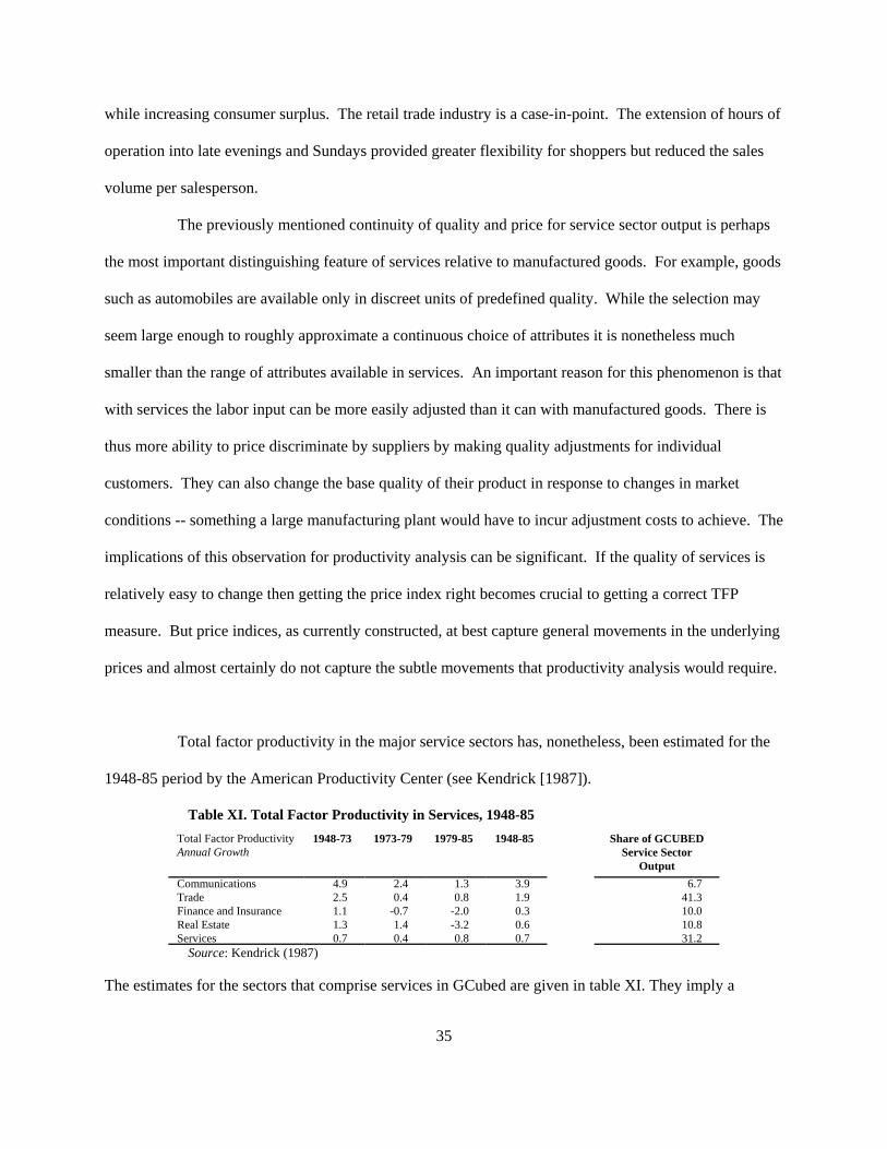
35

while increasing consumer surplus. The retail trade industry is a case-in-point. The extension of hours of

operation into late evenings and Sundays provided greater flexibility for shoppers but reduced the sales

volume per salesperson.

The previously mentioned continuity of quality and price for service sector output is perhaps

the most important distinguishing feature of services relative to manufactured goods. For example, goods

such as automobiles are available only in discreet units of predefined quality. While the selection may

seem large enough to roughly approximate a continuous choice of attributes it is nonetheless much

smaller than the range of attributes available in services. An important reason for this phenomenon is that

with services the labor input can be more easily adjusted than it can with manufactured goods. There is

thus more ability to price discriminate by suppliers by making quality adjustments for individual

customers. They can also change the base quality of their product in response to changes in market

conditions -- something a large manufacturing plant would have to incur adjustment costs to achieve. The

implications of this observation for productivity analysis can be significant. If the quality of services is

relatively easy to change then getting the price index right becomes crucial to getting a correct TFP

measure. But price indices, as currently constructed, at best capture general movements in the underlying

prices and almost certainly do not capture the subtle movements that productivity analysis would require.

Total factor productivity in the major service sectors has, nonetheless, been estimated for the

1948-85 period by the American Productivity Center (see Kendrick [1987]).

Table XI. Total Factor Productivity in Services, 1948-85Total Factor ProductivityAnnual Growth

1948-73 1973-79 1979-85 1948-85 Share of GCUBEDService Sector

OutputCommunications 4.9 2.4 1.3 3.9 6.7Trade 2.5 0.4 0.8 1.9 41.3Finance and Insurance 1.1 -0.7 -2.0 0.3 10.0Real Estate 1.3 1.4 -3.2 0.6 10.8Services 0.7 0.4 0.8 0.7 31.2

Source: Kendrick (1987)

The estimates for the sectors that comprise services in GCubed are given in table XI. They imply a

36

sectoral productivity growth (1948-85) of 1.4 percent annually for the GCubed Services sector. The

treatment of labor input in this table follows that of the Bureau of Labor Statistics in counting unadjusted

hours worked, thus changes in labor quality are treated as productivity increases rather than as increases

in the labor input.

Summary

The preceding discussion has outlined factors affecting productivity growth in a twelve sector

aggregation of the economy. We summarize productivity growth in those sectors by presenting a table of

the growth rates calculated from Jorgenson, Gollop and Fraumeni (1987) and Jorgenson and Kuroda

(1992):

Table XII. US Total Factor Productivity Estimates1950-59* 1960-69* 1970-79* 1980-85**

Electric Utilities 2.0 2.4 -1.7 -1.1Gas Utilities 0.3 0.8 -1.8 -1.1Petroleum Refining (2) 0.1 0.1 0.1 4.1Coal Mining 3.6 1.9 -5.2 -0.9Crude Oil & Gas Extraction 0.2 1.3 -7.9 Mining 0.4 0.2 -1.2 -0.9Agriculture 1.7 2.1 0.7 4.9Forestry & Wood ProductsDurable Manufacturing 1.0 0.6 1.1Non-Durable Manufacturing 0.7 0.2 0.4Transportation 1.4 0.6 0.5 0.8

1948-73 1973-79 1979-85Services 1.8 0.5 0.1

The Durable Manufacturing sector shown in table XII omits Electrical Equipment, Transportation

Equipment and Precision Instruments for the years 1980-85. The Non-durable Manufacturing sector

omits Tobacco Manufactures, Apparel and other fabricated textile products and Petroleum and Coal

products, again for the 1980-85 period.

V. Implementation of Productivity Growth in a 12 sector aggregation (The GCUBED Model)

The previous sections discussed productivity growth in various sectors of the US economy. It

would be useful to have a similar set of results for other countries so that international comparisons could

37

(7)

(8)

be made. Unfortunately, researchers in other countries have not shown as keen an interest as their U.S.

counterparts in measuring productivity growth so there is less work from which we can draw -- a partial

exception is found in Japan. The table on the following page (Table XIII) brings together estimates of

TFP growth from a number of studies to create a matrix of growth rates for the 12 sectors previously

discussed in a multi-region setting.

A stylized fact of technical change is that it has been Harrod-neutral in much of the post-world

war II era. We now translate the productivity growth of those studies to a Harrod-neutral measure of

technical change and combine it with labor force growth. Using the notation of section II and making the

assumptions outlined there we have:

where sk is the cost share of physical capital. The alternative formulation which is more explicity Harrod-

neutral is given by:

Table XIII. 12 Sectors

Electric Gas Petroleum Coal Crude Oil & Forestry & Durable Non-durableSource Country Period Utilities Utilities Refining Mining Gas Extraction Mining Agriculture Wood Prod Manuf. Manuf. Transp. Services

EM U.S. 1970-83 -4.28 -0.38 1.49 1.16 1.65 0.37JGF 1950-60 2.00 0.30 1.65 3.60 0.20 0.41 1.70 0.36 1.70 1.11 0.70JGF 1960-70 2.40 0.80 1.90 1.90 1.30 0.21 2.10 0.99 0.90 0.55 -0.08JGF 1970-79 -1.70 -1.80 -8.50 -5.20 -7.90 -1.05 0.70 0.33 -0.30 0.58 0.29JK 1960-70 2.11 2.11 1.62 1.08 1.18 0.36 0.73 1.09 0.40JK 1970-80 -1.47 -1.47 -4.56 -5.58 0.67 0.56 0.19 1.00 0.07JK 1980-85 -1.67 -1.67 3.42 0.05 4.43 1.04 0.50 0.25 0.27BLS 1960-70 1.46 1.09BLS 1970-80 1.07 0.52BLS 1980-85 1.44 1.03G 1960-73 1.54 1.54 0.34 0.23 1.97 1.97 2.53 0.38G 1973-79 0.21 0.21 -0.99 -1.10 0.64 0.64 1.20 -0.95G 1979-92 0.72 0.72 -0.48 -0.59 1.15 1.15 1.71 -0.44EM Japan 1970-83 1.60 -0.74 2.62 0.66 1.15 0.55JK 1960-70 3.22 3.22 -1.36 1.66 0.45 1.86 0.93 3.06 1.49JK 1970-80 -2.99 -2.99 -3.89 1.72 -1.64 0.80 0.19 0.49 0.05JK 1980-85 0.60 0.60 -1.29 0.30 -0.27 0.20 0.29 1.19 0.81EM Germany 1970-83 -2.43 3.08 1.60 0.62 0.52 1.37EM France 1970-83 1.97 0.89 2.06 0.85 0.85EM U.K. 1970-83 8.22 2.55 1.32 0.51 1.70 0.11EM Italy 1970-83 2.12 1.11 1.52 0.77 -0.13EM Canada 1970-83 0.17 1.77S 1957-79 -4.66RP 1967-80 0.94 0.94 -1.02 -0.04 -0.14 2.43 0.70 0.51 2.29 1.02EM Belgium 1970-83 2.50 0.51 3.27 -0.88 1.06EM Denmark 1970-83 3.26 0.83 2.68 -0.98 0.88EM Finland 1970-83 0.62 1.44 2.03EM Norway 1970-83 2.68 1.17 -0.48 2.46 0.34EM Sweden 1970-83 -2.62 1.22 2.84 -1.58 1.76 1.09EM Australia 1970-83 2.95 2.52M China 1980-85 -3.71 0.80 -0.82K 1961-85 7.00 7.00A India 1960-85 -0.13 -0.12 -0.14E Brazil 1950-80 2.55 2.25 2.25E 1960-80E Argentina 1950-80 0.44 1.05 1.05E 1960-80E Mexico 1950-80 1.84Z Africa 1960-80 1.60 0.30

E: Elias (1992) M: McGuckin et. al. (1992) JGF: Jorgenson, Gollop and Fraumeni (1987)RP: Rao and Preston (1984) A: Ahluwalia (1991) K: Kuan et. al. (1988)JK: Jorgenson and Kuroda (1995) S: Stollery (1985) Z: Zind (1992)EM: Englander & Mittlestadt (1987) G: Gordon (1995) BLS: Bureau of Labour Statistics Database

14See Appendix II for a sectoral mapping and for details of the aggregation.

39

(9)

(10)

Table XIVOutput Contrib. Contrib. Contrib. TFP Equivalent

Sector Growth of Capital of Labor of Interm. Input Growth LATCElectric Utilities 6.28 2.75 0.34 2.27 0.92 6.75Gas Utilities 5.31 1.06 0.24 4.03 -0.01 0.64Petroleum Refining 2.71 0.24 0.05 4.22 -1.79 -14.35Coal Mining 0.38 0.69 -1.16 1.12 -0.27 -0.30Crude Oil & Gas Extraction 2.13 1.04 0.31 2.91 -2.14 -17.05Mining 2.63 1.50 0.15 1.10 -0.14 -0.02Agriculture 2.20 0.42 -0.86 1.30 1.36 6.26Forestry & Wood Products 2.88 0.45 -0.11 2.45 0.09 1.13Durable Manufacturing 3.94 0.44 0.57 2.49 0.44 2.11Non-durable Manufacturing 3.54 0.37 0.20 1.93 1.03 4.80Transportation 2.93 0.52 0.07 1.39 0.94 3.93Services 4.05 0.59 0.78 2.21 0.46 1.97

Source: Authors’ calculations from data presented in Jorgenson, Gollop and Fraumeni (1987)

Where n is labor force growth. From this we get:

implying:

In Tables XIV and XV we have calculated this adjusted productivity growth term. In Table XIV

we use the data found in Jorgenson, Gollop and Fraumeni (1987) to perform this calculation on their

sectoral results14. The fourth column provides the recalculated Harrod-neutral labor-augmenting technical

change. In general the energy sectors have had slower productivity growth than the non-energy sectors

which, as is shown in Bagnoli, McKibbin and Wilcoxen (1995), has important implication for future

economic development if the trend should continue. To get Table XV we used population, labor force

and hours worked data to perform this calculation for the studies of Table II.

Table XV

Maddison (1989) Gordon (1995) BCC (1995) CRS (1986) BS (1995)Equiv. Equiv. Equiv. Equiv. Equiv.

Country Period LATC Country Period LATC Country Period LATC Country Period LATC Country Period LATC

U.S. 1950-73 U.S. 1960-73 1.93 U.S. 1960-70 2.14 U.S. 1960-73 1.86 U.S. 1960-90 0.481973-84 0.09 1973-79 -0.20 1970-80 0.29

1979-92 0.54 1980-86 1.14 1986-92 0.86

Japan 1950-73 Japan 1960-73 Japan 1960-70 7.29 Japan 1960-73 7.47 Japan 1960-90 3.041973-84 2.91 1973-79 1.84 1970-80 1.57

1979-92 2.33 1980-86 2.00 1986-92 1.86

France 1950-73 France 1960-73 5.20 France 1960-70 4.00 France 1960-73 3.91 France 1960-90 1.381973-84 0.87 1973-79 3.41 1970-80 1.86

1979-92 2.24 1980-86 1.29 1986-92 1.86

Germany 1950-73 Germany 1960-73 4.90 Germany 1960-70 3.57 Germany 1960-73 3.41 Germany 1960-90 1.411973-84 0.62 1973-79 3.84 1970-80 2.00

1979-92 2.06 1980-86 1.00 1986-92 2.14

U.K. 1950-73 U.K. 1960-73 3.31 U.K. 1960-70 1.57 U.K. 1960-73 2.57 U.K. 1960-90 1.171973-84 -0.12 1973-79 1.66 1970-80 1.00

1979-92 1.74 1980-86 2.86 1986-92 0.29

Canada 1960-73 3.38 Canada 1960-70 2.57 Canada 1960-73 1.30 Canada 1960-90 0.061973-79 0.53 1970-80 1.43 1979-92 -0.06 1980-86 1.14

1986-92 -0.57 Italy 1960-73 8.18 Italy 1960-70 5.71 Italy 1960-73 4.24 Italy 1960-90 2.56

1973-79 3.87 1970-80 2.86 1979-92 2.51 1980-86 1.00 1979-92 1986-92 1.57

Australia 1960-70 2.57 1970-80 1.14 1980-86 1.00 1986-92 1.00

China 1950-73 3.15 China 1960-70 2.83 1973-84 6.03 1970-80 2.17

1980-86 7.67 1986-92 5.17

Korea 1950-73 7.19 Korea 1960-70 2.67 Korea 1960-73 9.81 Korea 1966-90 7.621973-84 5.66 1970-80 2.33

1980-86 5.50 1986-92 4.50

Taiwan 1950-73 11.67 Taiwan 1960-70 3.33 Taiwan 1955-60 6.95 Taiwan 1966-90 9.031973-84 8.00 1970-80 3.33

1980-86 4.00 1986-92 5.17

India 1950-73 -9.08 India 1960-70 1.33 India 1960-79 6.21 1973-84 2.63 1970-80 0.33

1980-86 3.50 1986-92 3.17

Argentina 1950-73 2.88 Argentina 1960-70 2.33 Argentina 1960-74 5.28 Argentina 1940-80 2.051973-84 -1.45 1970-80 0.33

1980-86 -3.00 1986-92 2.17

Brazil 1950-73 4.81 Brazil 1960-70 3.00 Brazil 1960-74 9.50 Brazil 1940-80 2.591973-84 0.08 1970-80 4.17

1980-86 -1.17 1986-92 -3.67

Chile 1950-73 2.18 Chile 1960-70 2.67 Chile 1960-74 5.25 Chile 1940-80 2.351973-84 -0.47 1970-80 0.50

1980-86 -2.67 1986-92 6.83

Mexico 1950-73 4.23 Mexico 1960-70 3.50 Mexico 1960-74 6.42 Mexico 1940-80 3.171973-84 1.24 1970-80 0.83

1980-86 -4.83 1986-92 0.17

USSR 1950-73 2.39 1973-84 -0.64

Note: BCC- Bosworth, Collings and Chen; CRS-Chenery, Robinson and Syrquin; BS-Barro and Sala-i-Martin

41

(12)

(13)

(14)

The GCUBED model uses a CES production function so that unit elasticity is not imposed on the

data. When implementing the LATC illustrated in table XIV in a parameterized model with fixed shares

we need to be aware of some pitfalls. To illustrate further, we specify Harrod-neutrality in a CES

function:

In this case, letting q be the price of output and w and r be the wage and the price of capital, respectively,

we use the profit maximization conditions: :

Productivity growth becomes:

Now, in the CES production function 1/(1+D) is the elasticity of substitution. Equations (13) and (14),

therefore, imply that for a given change in output and inputs the measurement of productivity growth is

related to the elasticity. It can be shown that this relationship has a tendency to be negative (the

relationship is negative for the U.S. and is most likely to be negative in industrialized countries) so that as

the elasticity becomes larger the rate of productivity growth that is calculated will decrease. This result is

important for single country studies where measurement of the level of productivity growth is desired but

it is even more important in comparative studies across very different economies where the substitution

elasticities may differ. Researchers find elasticities of substitution much less than one for the

industrialized countries (see Yuhn [1991] for a survey of U.S. empirical work). De La Grandville (1989),

however, has proposed that the elasticity of substitution might be closer to unity in the developing

countries -- or at least higher than in industrialized countries. Some empirical work has supported this

42

proposition (see Yuhn [1991]). In other words, studies which do cross-country TFP calculations using

Cobb-Douglas production functions are, at the very least, obliged to provide some justification for their

assumption of unit elasticity because there is a potentially strong bias in the results originating in that

assumption.

IV. Concluding Remarks

This paper reviewed some issues in productivity measurement from a growth accounting

perspective. We illustrated the basic techniques of productivity growth measurement and surveyed both

aggregate and sectoral measurements undertaken by other authors. It was pointed out that there are

numerous areas of weakness in the measures so there is reason to be skeptical that any one measure of

productivity growth accurately reflects economic changes. However, as was pointed out in Baily and

Gordon (1988), the current measurements are accurate enough to provide a rough of gauge of actual

productivity growth.

The sectoral productivity growth survey that we undertook provides some interesting

observations on the components of aggregate growth. It was argued in Jorgenson (1987) that changes in

the allocation of factors of production can have important influences on growth rates without requiring

any changes in either composition or quantity of the factors. The reason for this is that movement of

factors from low to high value sectors will, by itself, give you measured increases in output. We saw in

the sectoral data considerable differences in productivity growth among sectors so there is scope for this

phenomenon to be occuring. We also saw, however, that productivity growth and other sectoral

indicators can be greatly affected by one-time or transitory events -- undermining arguments regarding

the importance of observed sectoral differences. The obvious conclusion we draw from this is that a

careful analysis should combine both sectoral and aggregate data with a strong emphasis on eliminating

short-term influences when the sectoral differences have important long-term implications.

43

References

Akerlof, G. A., W. T. Dickens and G. L. Perry (1996), “The Macroeconomics of Low Inflation,” Brookings Papers on Economic Activity.

Aivazian, V. A., J. L. Callen, M.W. Chan and D. C. Mountain (1987), “Economies of Scale Versus Technological Change in the Natural Gas Transmission Industry,” Review of Economics andStatistics, vol. 69(3), August, pp. 356-61.

Ahluwalia, I.J. (1985), “Industrial Growth in India: Performance and Prospects”, Journal of Development Economics, vol. 23, no. 1, September, pp. 1-18.

Ahluwalia, I.J. (1991), Productivity and Growth in Indian Manfacturing, New York: Oxford University Press.

Baily, M.N. and R. J. Gordon (1988), “The Productivity Slowdown, Measurement Issues, and theExplosion of Computer Power,” Brookings Papers on Economic Activity, pp. 347-420.

Barro, R., and Sala-i-Martin (1995), Economic Growth, New York, N.Y.: McGraw-Hill.

Baumol, W. J. (1986), “Productivity Growth, Convergence, and Welfare: What the Long-run DataShow,” American Economic Review, Vol. 76, no. 5, pp. 1072-85.

Bosworth, B., S. M. Collins and Y. Chen (1995), “Accounting for Differences in Economic Growth,”Conference paper: Structural Adjustment Policies in the 1990's: Experience and Prospects,November 5-6, (1995). Institute for Developing Economies, Tokyo, Japan.

Chenery, H., S. Robinson and M. Syrquin (1986), Industrialization and growth: A Comparative Study,New York: Oxford University Press.

Christensen, L. R., and D. W. Jorgenson (1969), “The Measurement of U.S Real Capital Input,1929-1967," Review of Income and Wealth, Series 15, no. 4, pp. 293-320.

Christensen, L. R., D. Cummings and D. W. Jorgenson (1980), “Economic Growth, 1947-1973: AnInternational Comparison” In New Developments in Productivity Measurements, eds. John W.Kendrick and Beatrice Vaccara, 595-698. NBER Studies in Income and Wealth, vol. 41, NewYork: Columbia University Press

Costello, D. M. (1993), “A Cross-Country, Cross-Industry Comparison of Productivity Growth,” Journalof Political Economy, vol. 101(2), pp. 207-222.

Denison, E. F. (1962), Sources of Economic Growth and the Alternatives Before Us. New York:Committee for Economic Development

Denison, E. F. (1967), Why Growth Rates Differ, Washington, D.C.:The Brookings Institution.

44

Denison, E. F. (1979), Accounting for Slower Growth: The United States in the 1970's, Washington,D.C.: The Brookings Institution.

Diewert, W. E. (1976), “Exact and Superlative Index Numbers,” Journal of Econometrics, vol. 4, pp. 115-145.

Diewert, W. E. (1992), “The Measurement of Productivity,” Bulletin of Economic Research, vol. 44(3),pp.163-98.

De La Grandville, O. (1989), “In Quest of the Slutsky Diamond,” American Economic Review, vol.79(3), June, pp. 468-81.

Elias, V.J. (1992), Sources of Growth: A Study of Seven Latin American Economies, San Francisco: ICS Press.

Englander, A. S., and A. Mittelstadt (1988), “Total Factor Productivity: Macroeconomic and StructuralAspects of the Slowdown,” OECD Economic Studies, No. 10, spring, pp. 7-56.

Feenstra,R.C., and J. R. Markusen (1994), “Accounting for Growth with New Inputs” InternationalEconomic Review vol. 35(2), May, pp. 429-47.

Friedman, B. L. (1992), “Productivity in Crude Oil and Natural Gas Production,” Monthly Labor Review, March, pp.9-17.

Glaser, G. L. (1993), “Multifactor Productivity in the Utility Services Industries,” Monthly LaborReview, May, pp. 34-49.

Gordon, R. J. (1991), “Productivity in the Transportation Sector,” NBER Working Paper No. 3815, February.

Gordon, R. J. (1992), “Forward into the Past: Productivity Retrogression in the Electric GeneratingIndustry,” NBER Working Paper No. 3988, February.

Gordon, R. J. (1995), “Is There a Tradeoff Between Unemployment and Productivity Growth,”NBER Working Paper No. 5081, April.

Gullickson, W. (1992), “Multifactor Productivity in Manufacturing Industries,” Monthly Labor Review, October, pp.20-32.

Summers, R., and A. Heston (1980), “International Comparisons of Real Product and Its Composition:1950-77,” Review of Income and Wealth, vol. 26(1), March, pp. 19-66.

Hibdon, J. E. And M. J. Mueller (1990), “Economies of Scale in Petroleum Refining, 1947-1984: A Survivor Principle-Time Series Analysis,” Review of Industrial Organization, vol. 5(3), pp. 25-43.

Jorgenson, Dale W., (1984), “The Role of Energy in Productivity Growth,” In Kendrick, John W., ed,International Comparisons of Productivity and Causes of the Slowdown, Cambridge: Ballinger,

45

pp.270-323.

Jorgenson, Dale W., (1988), “Productivity and Postwar U.S. Economic Growth,” Journal of Economic Perspectives, vol. 2(4) Fall, pp. 24-41.

Jorgenson, D. W., and B. M. Fraumeni (1981), “Relative Prices and Technical Change”,in Modellingand Measuring Natural Resource Substitution, eds. E. R. Bernst and B. C. Field, Cambridge:MIT Press.

Jorgenson, D. W., and B. M. Fraumeni (1992), “Investment in Education and U.S. Economic Growth”, Scandinavian Journal of Economics, vol. 94, Supplement. pp. 51-70.

Jorgenson, D. W., and F. M. Gollop (1992), “Productivity Growth in U.S. Agriculture: A Postwar Perspective”, American Journal of Agricultural Economics, pp. 745-50.

Jorgenson, Dale W., Frank M. Gollop, and Barbara M. Fraumeni, (1987), Productivity and U.S.Economic Growth, Cambridge, Harvard University Press.

Jorgenson, D. W., and M. Kuroda (1992), “Productivity and International Competitiveness in Japan andthe United States, 1960-1985”, The Economic Studies Quarterly, vol. 43(4), pp. 313-325.

Kendrick, J. W. (1987), “Service Sector Productivity,” Business Economics, vol. 22(2), pp. 18-24.

Krugman, P.R. (1994) “Competitiveness: A Dangerous Obsession,” Foreign Affairs, 73(2),March-April, pp. 28-44.

Kruvant, W. J., C. E. Moody, Jr. and P. L. Valentine (1982), “Sources of Productivity Decline in U.S.Coal Mining, 1972-1977,” The Energy Journal, vol. 3(3), pp. 53-70.

Kuan, E., et. al., (1988), “Prodcutivity Changes in Chinese Industry, 1953-1985”, Journal ofComparative Economics, vol. 12, pp. 570-591.

Kuroda, M., K. Yoshioka and D. W. Jorgenson (1992), “Relative Price Changes and Biases of TechnicalChange in Japan”, The Economic Studies Quarterly, vol. 35(2), pp. 116-38.

May, J. D., and M. Denny (1979), “Factor-Augmenting Technical Progress and Productivity in U.S.Manufacturing,” Internatinoal Economic Review, vol. 20, pp. 759-74.

Maddison, A. (1987), “Growth and Slowdown in Advanced Capitalist Economies: Techniques of Quantitative Assessment”, Journal of Economic Literature, vol. 25, June, pp. 649-98.

Maddison, A. (1989), The World Economy in the 20th Century, OECD, Development Centre Studies.

Mark, J. A. (1982), “Measuring Productivity in Service Industries,” Monthly Labor Review, June, pp.3-8.

McGuckin, R. H., et. al., (1992), “Post-Reform Productivity Performance and Sources of Growth inChinese Industry: 1980-85," Review of Income and Wealth, Series 38, Numer 3. September.

McKelvey, V. E. (1960). "Relation of Reserves of the Elements to Their Crustal Abundance."

46

American Journal of Science, Vol. 258-A, pp. 234-41.

McKibbin, W. J. and P. J. Wilcoxen (1995). “The Theoretical and Empirical Structure of GCUBED”,Brookings Discussion Papers in International Economics, No. 118, The Brookings Institution.

Millward, R. (1990), “Productivity in the UK Services Sector: Historical Trends 1856-1985 and Comparisons with the USA 1950-85,” Oxford Bulletin of Economics and Statistics, vol 52(4),pp.423-36.

Mulligan, C. B. and X. Sala-i-Martin (1995). “Measuring Aggregate Human Capital,” NBER WorkingPaper No. 5016, February.

Nerlove, M. (1965), Estimation and Identification of Cobb-Douglas Production Functions, Chicago:Rand-McNally.

Nordhaus, W.D. (1972) “The Recent Productivity Slowdown,” Brookings Papers on Economic Activity, pp. 493-536.

Nordhaus, W.D. (1988) “The Productivity Slowdown, Measurement Issues, and the Explosion ofComputer Power: Comment,” Brookings Papers on Economic Activity, pp. 421-24.

Rao, P.S. and R.S. Preston (1983), “Interfactor substitution and total factor productivity growth:Evidence from Canadian industries,” Economic Council of Canada, Discussion Paper No. 242.

Romer, P.M. (1990), “Endogenous Techonological Change,” Journal of Political Economy, vol. 95(5), pp. 71-102.

Shoesmith, G. L. (1988), “Economies of Scale and Scope in Petroleum Refining”, Applied Economics,vol. 20, December, pp. 1643-52.

Sickles, R. C., and M. L. Streitwieser (1992), “The Structure of Technology, Substitution, andProductivity in the Interstate Natural Gas Transmission Industry under the NGPA of 1978,”Bureau of the Census Center for Economic Studies Discussion, Working Paper 92-9, August.

Sider, H. (1982) “Safety and Productivity in Underground Coal Mining” The Review of Economics and Statistics, vol. 65(2), May, pp. 225-33.

Solow, Robert M., (1957), “Technical Change and the Aggregate Production Function,” Review of Economics and Statistics, vol. 39(3), 1957, August, pp. 312-20.

Solow, Robert M., (1960), “Investment and Technical Progress,” in Mathematical Models in the SocialSciences, 1959, eds. Arrow, K.J., S. Karlin and P. Suppes, Stanford: Stanford University Press

Stollery, K. R. (1985), “Productivity Change in Canadian Mining 1957-1979”, Applied Economics, vol.17, pp. 543-558.

Young, A. (1994), “Lessons from the East Asian NICS: A Contrarian View”, European EconomicReview, vol. 38, April, pp. 964-73.

47

Yuhn, K. H. (1991), “Economic Growth, Technical Change Biases, and the Elasticity of Substitution:A Test of the De La Grandville Hypothesis,” Review of Economics and Statistics, vol. 73(2), pp.340-46.

Zind, R. G., (1992), “Factors Contributing to Productivity Growth in the LDCs”, Economic Notes, vol.21, no. 1, pp. 120-136.

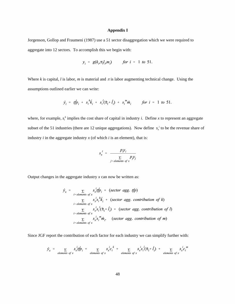
48

Appendix I

Jorgenson, Gollop and Fraumeni (1987) use a 51 sector disaggregation which we were required to

aggregate into 12 sectors. To accomplish this we begin with:

Where k is capital, l is labor, m is material and B is labor augmenting technical change. Using the

assumptions outlined earlier we can write:

where, for example, sik implies the cost share of capital in industry i. Define x to represent an aggregate

subset of the 51 industries (there are 12 unique aggregations). Now define sxi to be the revenue share of

industry i in the aggregate industry x (of which i is an element), that is:

Output changes in the aggregate industry x can now be written as:

Since JGF report the contribution of each factor for each industry we can simplify further with:

49

where cij is the contribution of factor j in industry i. This equation forms the basis for the calculations

reported in table XIV.