PRODUCTIVE STRUCTURE AND TRADE RELATIONS: … · Productive Structure and Trade Relations: ... unit shipping cost and fluctuations in exchange rates, ... Acre, Amazonas and Roraima,

PRODUCTIVE STRUCTURE AND TRADE RELATIONS:

THE CASE OF THE WESTERN BORDER REGIONS OF

PARANÁ STATE, BRAZIL

Carlos Alberto Gonçalves Júnior

Joaquim José Martins Guilhoto

TD Nereus 09-2015

São Paulo

2015

1

Productive Structure and Trade Relations:

The Case of the Western Border Regions of Paraná State, Brazil

Carlos Alberto Gonçalves Júnior and Joaquim José Martins Guilhoto

Abstract. The aim of this paper is to analyze the productive structure and the trade

relations, national and international, of the Western Border Regions of Paraná state in

Brazil. As so, based on the input-output database from the University of São Paulo

Regional and Urban Economics Lab – NEREUS, we have estimated: a) an interregional

input-output model for 6 regions (5 in Paraná and the remaining of Brazil), for 2008;

and b) the external trade relations of these regions. The results also point out the

importance for the Western border regions of traditional sectors of the state economy,

however, in some situations, the sectors that most contribute to output, income, value

added, and employment generate many of these benefits outside the regions, mainly due

to the spillovers. These findings certainly need to be considered by policy makers when

designing policies for the development of the analyzed region.

1. Introduction

Paraná is one of the major states of Brazil regarding agricultural and industrial

production. According to IPARDES (2013) Paraná's economy is the fifth largest in the

country. The state production represents 5.84% of the national GDP, with a per capita

income of R$ 20,800 in 2010, above the national average of R$ 19,700. The Value

Added for Paraná state is divided into 8.48% from agriculture, 27.46% from industry

and 64.06% from trade and services.

In 2012, the share of Paraná in the national exports was 7.3%, the fourth position among

the Brazilian states. Regarding imports, the largest suppliers of goods to Paraná were

China, Nigeria, Argentina and the United States, amounting to US$ 8.6 billion.

Besides the importance for the country's economy, Paraná has a peculiar feature, with

the presence of 139 municipalities in the "Western border strip", setting limits with

Paraguay and Argentina. This feature requires from Paraná policy makers differentiated

strategies to promote the growth and the development of this region, due to specific

characteristics of these municipalities caused by the proximity from the border, or by

the distance of this region from major economic centers of the state and the country.

2

In this context, the aim of this paper is to analyze: a) the economic structure of the

Western border region of Paraná, pointing out their similarities and their differences

with the rest of the country; b) the interdependence of the regions, concerning

production, employment and value added, and identifies how production can spill over

from one region to another and to the rest of the country; c) identify the relationship of

the Western border region of Paraná State with neighboring countries, Paraguay and

Argentina.

The paper highlights the importance of identifying sectors where the stimulus to

regional final demand increases production, mostly within the border regions, and also

to identify sectors where the increasing in the national final demand can spill over

dynamism to the economy of the border region.

In order to achieve the proposed objective, the paper, besides this introduction, is

divided into 6 other sections. In section 2 the characterization of the border region is

presented. In section 3 some concepts of regions and regional development are

approached. Section 4 presents the methodological aspects, and the database is

presented in section 5. The results are presented in section 6, while the final comments

are made into the last section.

2. Concept and Characterization of the Border Region

The meaning of “border” may be associated with the common sense of the end of a

country or region, mingling with the concept of limit. To Hissa (2002) the limit, as

territory, is facing inwards. On the other hand, the border view from the same place, is

facing outwards. The limit encourages the idea of distance and separation, while the

border moves reflection about the contact and integration.

To Rolim (2004) places on the border, while permitting a common economic space,

establish barriers to integration, i.e., provide conditions for the existence of a flow of

people, capital and at the same time create restrictions so that it can happen. Parsley and

Wei (2000) analyze the volatility of prices in a three-dimensional panel data with 27

products, 88 quarters across 96 cities in the U.S. and Japan. The results showed a very

high volatility of relative prices. The high volatility in prices is attributed to factors such

3

as distance, unit shipping cost and fluctuations in exchange rates, which are known in

the literature as "border effect".

Turrini and Ypersele (2010) investigated the role played by differences in the judicial

system to deal with "border effect". In this context, the asymmetries in the procedures to

resolve trade disputes contribute greatly to reducing the trade between two cities with

the presence of an international border between them.

Morshed (2003) shows that the variation of the prices in equidistant cities located in two

different countries is systematically larger than that for the cities within the same

country. The Nontariff barriers and exchange rate variability are the proximate causes

of this systematic difference in consumer price variability. The author, using data from

developing countries with large nontariff barriers and more volatile exchange rate

suggests that those claims are overemphasized in these countries.

Despite the relevance of the "border effect" Holmes and Stevens (2012) related

distance, the presence of borders and the size of the company to explain the difficulties

of trade between regions. According to the authors, the fact that large manufacturing

plants export relatively more than small plants has been the foundation of much work in

the international trade literature. However, they show that this fact is not entirely an

international trade phenomenon.

They examined this hypothesis using Census microdata on plant shipments from the

Commodity Flow Survey and found that part of this effect can be due to the distance

effect, apart from any border effect. Export destinations tend to be farther than domestic

destinations, and large plants tend to ship farther distances, even to domestic locations

compared with small plants.

Portes and Rey (2005) using a panel data set of bilateral gross cross-border equity flows

between 14 countries in the period of 1989–1996 found that the gross transaction flows

depend on market size in source and destination countries, as well as trading costs, in

which both information and the transaction technology play a role. They say that the

geography of information is the main determinant of the pattern of international

transactions.

4

Leasing Jr. and Azevedo (2009) analyzed the border effect in Brazil and found that,

despite the country having participated in major trade agreements, such as Mercosur,

still has a high border cost. The results indicate that trade among Brazilian states is 33

times higher than the international trade of these states, in the specific case of Paraná,

for the year 1999, the intra-national trade accounted for 86.09% of the total trade in the

state.

In Brazil, mainly for strategic purposes of national security, the Brazilian Institute of

Geography and Statistics - IBGE considers "border" a 150Km strip along the border,

parallel to the landline part of the national territory. In this region, it is forbidden to

grant lands, open transport routes, build bridges and airfields and install media, besides

the exploration of industries which represent a threat to the national security needs a

special authorization from the federal government.

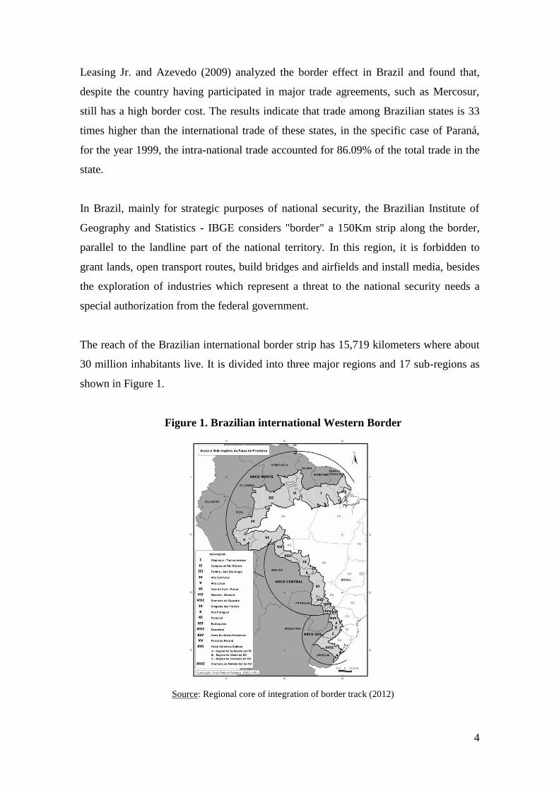
The reach of the Brazilian international border strip has 15,719 kilometers where about

30 million inhabitants live. It is divided into three major regions and 17 sub-regions as

shown in Figure 1.

Figure 1. Brazilian international Western Border

Source: Regional core of integration of border track (2012)

5

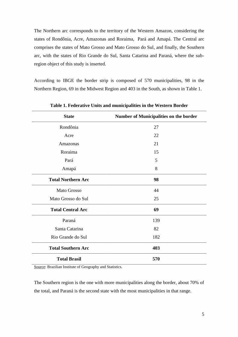
The Northern arc corresponds to the territory of the Western Amazon, considering the

states of Rondônia, Acre, Amazonas and Roraima, Pará and Amapá. The Central arc

comprises the states of Mato Grosso and Mato Grosso do Sul, and finally, the Southern

arc, with the states of Rio Grande do Sul, Santa Catarina and Paraná, where the sub-

region object of this study is inserted.

According to IBGE the border strip is composed of 570 municipalities, 98 in the

Northern Region, 69 in the Midwest Region and 403 in the South, as shown in Table 1.

Table 1. Federative Units and municipalities in the Western Border

State Number of Municipalities on the border

Rondônia 27

Acre 22

Amazonas 21

Roraima 15

Pará 5

Amapá 8

Total Northern Arc 98

Mato Grosso 44

Mato Grosso do Sul 25

Total Central Arc 69

Paraná 139

Santa Catarina 82

Rio Grande do Sul 182

Total Southern Arc 403

Total Brasil 570

Source: Brazilian Institute of Geography and Statistics.

The Southern region is the one with more municipalities along the border, about 70% of

the total, and Paraná is the second state with the most municipalities in that range.

6

The Western border of Paraná consists of 139 municipalities, representing 35% of

municipalities in the state. Concerning the population, the region has about 2.3 million

inhabitants, which corresponds to 23% of Paraná population, as presented into Table 2.

Table 2. Population and GDP for Paraná and Western Border of Paraná in 2010

State

Municipalities

Border

Municipalities

Variables Total Average Total Average

GDP (R$ million) 217,290 545 41,790 303

Population

(Thousand) 10,445 26 2,369 17

Source: IPARDES (2013)

The Western border of Paraná is also relevant to the state's economy, accounting for

about 20% of the state GDP. However, according to Rolim (2004), this region is far

from the major Brazilian urban centers and large cities in South America. Even

considering the Metropolitan Region of Curitiba, which is the capital and the industrial

center of Paraná, there is a distance of at least 636 km from Foz do Iguaçu, the most

border city, to the state capital.

In addition to the distance from the major production centers of the state and the

country, there is the "border effect" which also restricts the relationship of the

municipalities of the Western border of Paraná with the cities in the neighboring

countries (Paraguay and Argentina). As a result, the region is in itself quite complex

whit specific economic and administrative conditions.

Regarding the Brazilian side, which is the object of this study, it is possible to

emphasize the presence of three highly relevant factors for the region: (1) the Itaipu

hydroelectric plant, which, besides generating a large number of jobs, pays royalties for

some municipalities in the region that had their space flooded by the dam construction;

(2) the trade with Paraguay, especially the wholesales; and (3) the great tourism

potential of Foz do Iguaçu municipality.

7

In this context, given its economic specificity, the Western border of Paraná requires

particular strategies to promote its development, driven by regional actors and, mainly,

by efficient public policies, which could promote equitable development and income

distribution in the region.

To better understand these concepts, the next section of this study will address some

theories that analyze the conditions under which the development takes place in a

region, how it happens and spreads regionally.

3. The Region and the Regional Development

As already mentioned, the Western Border was determined by the State as a strategic

space for national security purposes, however, the concept of region goes beyond the

space determined by the State.

According to Souza & Gemelli (2011) region is a reality that is materialized through the

social actors, appearing when the similarities and common internal relations are defined.

It also evidences the economic, social and cultural intra and inter dependencies, which

can be established by contiguity or by network formation.

For Hirschman (1977) economic progress does not occur at the same time and

everywhere in a region, there are forces that cause the spatial concentration of growth

around the points where it starts, but the economic progress can be transmitted inter-

regionally and internationally, i.e., since the growth becomes strong in a region, it

triggers certain forces that act on the remaining parts.

The region's economic growth causes a series of repercussions in other regions, because

of the interdependencies established by contiguity or by network formation, some

repercussions are favorable, others adverse. The favorable effects are called "fluency

effect", which are mainly composed by the effect of the increase in purchases and

investments in a region because of the growth that happens in another region. However,

this will only occur if there is a complementary relationship between economic regions.

On the other hand, to Hirschman (1977), the growth of a region can bring harm to other

regions, such as the migration of skilled labor and capital to the region where the

8

growth takes place, leaving the original regions. It happens when sectors in different

regions compete for the same resources.

According to Williamson (1977) this effect can be potentialized because the labor

migration is extremely selective, due to the prohibitive cost of migration for people with

low income levels, thus, during the migration process, regions lose workers with higher

qualification. Regarding the capital, a developed banking system can accelerate the

process of capital concentration, i.e., banks can raise funds from savers in a region and

redirect them to the region where the growth process is more advanced.

For Hirschman (1977) regional allocation of public investment is the most obvious way

in which economic policies influence the growth rates of the various regions of a

country. But this is not a trivial task, according to Williamson (1977), the declared or

covert intention of the federal government, to maximize national development, can

further increase the degree of regional inequality.

For Souza (2005) the strategy of polarizing the development was the main rule of the

Regional Planning in several countries, because the pulverized investment weakens the

linkage effects between sectors. The idea is to concentrate investments in specific points

in an attempt to serve the economic interests.

This way, Hirschman (1977) defines "great institutional measures" as arrangements that

enhance the fluency effect, i.e., the investments at the poles should flow to the

periphery, and mitigate the polarization effect, therefore, avoiding income concentration

in the richest regions.

To Sonis et al (1997) most studies that deal with trade between regions focus on

explaining trade flows, while little attention has been given to the geographical structure

of these flows, which is the goal of this study.

In summary, this study emphasizes the importance of analyzing the economic structure

of each region and identifying the relationships of complementary and inter-regional

competition, in order to show how the investment in a particular industry, in a particular

region, can "spill over" to the other regions and promote the "fluency effect ".

9

In addition, if the interest of policy makers is to develop the peripheral regions, it is

very important to identify which are the sectors where the investments are kept in the

peripheral regions and if there is no "spill over" to the poles, to avoid the income

concentration in richer regions (polarization effect). This information can guide the

policy makers in promoting efficient national strategies, without increasing regional

inequalities.

To Sonis et al (1997) the availability of information as contained in the input-output

matrices can help to understand the process of spatial and structural changes in a

particular region.

Baumol and Wolff (1994) point out the key role of input-output analysis in policy

formulation, highlighting the efficiency of this analysis of the rational use of scarce

resources.

4. Methodology

The input-output model developed by Leontief (1951) shows the flows of goods and

services among the sectors and agents of the economy for a given year. The inter-

industries flows are determined by economic as well as technological factors and can be

expressed through a system of simultaneous equations (Miller and Blair, 2009).

In matrix terms the inter-industries flows in the economy can be represented by

AX Y X (1)

Where:

X is a vector (n x 1) and it contains the value of total production by sector;

Y is also a vector (n x 1) and it contains the final demand values;

and A is a (n x n) matrix which contains the production technical coefficient.

In the model above, the final demand vector is usually considered exogenous to the

system; thus, the total production vector is determined only by the final demand vector,

which is given by:

10

BXY (2)

1

B I A

(3)

Where:

B , the Leontief inverse, is a (n x n) matrix of direct and indirect coefficients, in which

the element bij shows the total amount of production that is required from sector i to

produce one unit of final demand of sector j.

From equation (3) one can estimate the output multipliers of type (I), which shows the

direct and indirect effects for a given sector (Miller and Blair 2009), i.e., the total

amount of production generated in the economy to produce one unit of final demand of

the given sector, and is given by:

n

i

ijj bP1

(4)

Where:

jP is the output multiplier of sector j.

One can also estimate, for each sector in the economy, the total amount of employment,

value added, emissions, etc, that is generated directly and indirectly in the economy to

produce one unit of final demand of the given sector. In order to do so, one needs to

calculate the direct coefficient of the variable of interest:

i

i

iX

Vv (5)

Where:

iv is the direct coefficient of the variable of interest of sector i;

11

iV is the total of the variable of interest corresponding to sector i (for example, total

employment of sector i);

and iX is the value of total production of sector i.

Then, the total impact, direct and indirect, on the variable of interest will be given by:

i

n

i

ijj vbGV

1

(6)

where jGV

is the generator of the variable of interest corresponding to sector j, which

represents the total impact, direct and indirect, on the variable of interest given a new

final demand of one monetary unit in sector j.

Based on the Leontief system other indicators can be estimated and used to better

understand the economic relations and the productive structure of a given economy. In

this way, this paper makes use of backward and forward linkages (Hirschman-

Rasmussen and Pure), to better understand the productive structure of the Brazilian

economy. These indicators are described and defined in the following sections.

4.1. The Hirschman-Rasmussen Approach

The work of Rasmussen (1956) and Hirschman (1958) led to the development of indices

of linkage that have now become part of the generally accepted procedures for

identifying key sectors in the economy. Being ijb a typical element of the Leontief

inverse matrix, B ; *B the average value of all elements of B , and B j associated

typical column sums, then the backward linkage index can be defined as follows:

*/]/[ BnBU jj (7)

Defining F as the matrix of row coefficients derived from the matrix of intermediate

consumption, G as the Ghosh matrix given by 1 FIG (Miller and Blair, 2009),

12

*G as the average of all elements of G, and Gi* as being the sum of a typical row of G,

the forward linkages can be defined as:

*

* / GnGU ii (8)

The Hirschman-Rasmussen indices of linkages measure the importance of a sector in

the economy in terms of buyer (backward) or supplier (forward) of inputs. The Pure

linkage approach presented below is similar to the Hirschman-Rasmussen, however it

also takes into consideration the total production value of each sector in the economy,

i.e., the size of the sector. The sectors indicated as the most important inside the

economy, using the Pure linkage, in general are sectors with a great interaction among

the other sectors and with a significant level of production.

In general the Hirschman-Rasmussen are concerned mainly with the technical

coefficients, while the pure linkage also take into consideration the importance of the

values supplied and demanded by each economic sector.

4.2. The Pure Linkage Approach

As presented by Guilhoto, Sonis and Hewings (2005) the pure linkage approach can be

used to measure the importance of the sectors in terms of production generation in the

economy.

Consider a two-region input-output system represented by the following block matrix,

A, of direct inputs:

rj

rrrj

jrjj

rrrj

jrjjAA

A

A

A A

A A

A AA

0

00

0 (9)

Where:

Ajj and Arr are the quadrate matrices of direct inputs within the first and second region

and Ajr ;

13

and Arj are the rectangular matrices showing the direct inputs purchased by the second

region and vice versa.

From (7), one can generate the following expression:

IA

AI

BB

BBAB

jrj

rjr

r

j

rr

jj

rrrj

jrjj

Δ

Δ

Δ0

0Δ

Δ0

0ΔI

1 (10)

Where:

1

1

1

1

jrjrjjrr

rjrjrjjj

rrr

jjj

AAI

AAI

AI

AI

From equation (8) it is possible to reveal the process of production in an economy as

well as derive the Pure Backward Linkage (PBL) and the Pure Forward Linkage (PFL),

i.e.,

PBL = rArjjYj (11)

PFL = jAjrrYr (12)

Where the PBL will give the pure impact on the rest of the economy of the value of the

total production in region, i.e., the impact that is free from a) the demand inputs that

region j makes from region j , and b) the feedbacks from the rest of the economy to

region j and vice-versa. The PFL will give the pure impact on region j of the total

production in the rest of the economy

Other advantage of the Pure linkages in relation to the Hirschman-Rasmussen linkages

is that it is possible to get the Pure Total linkage in the economy (PTL) by adding the

PBL and the PFL, given that this index are measured in current values, i.e.,

14

PTL = PBL + PFL (13)

To facilitate a comparative analysis of the pure linkages with the Hirschman-Rasmussen

linkages one can do a normalization of the pure linkages. This normalization is done by

dividing the pure linkage in each sector by the average value of the pure linkage for the

whole economy, in such a way that the pure linkages normalized are given by the

following equations for the backward (PBLN), forward (PFLN) and total (PTLN)

linkages:

nPBLPBLPBLNn

i

iii

1

(14)

nPFLPFLPFLNn

i

iii

1

(15)

nPTLPTLPTLNn

i

iii

1

(16)

5. Database

As already mentioned, the Western border of Paraná is formed by 139 municipalities

positioned in an inner strip of 150 km, parallel to the landline part of the national

territory. Aiming to better analyze the Western border regions of Paraná state, and

understand how this region relates to itself, with the rest of Paraná, Brazil and the

World, the state of Paraná was divided into five regions (three border regions:

municipalities with distance from 0-50Km (R1), 50-100Km (R2), and 100-150Km (R3)

from the border, a central region (R4), and a seaside region (R5), besides a region called

remaining of Brazil (R6), shown in Figure 2.

15

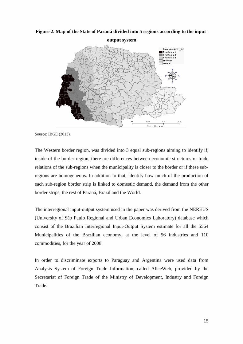
Figure 2. Map of the State of Paraná divided into 5 regions according to the input-

output system

Source: IBGE (2013).

The Western border region, was divided into 3 equal sub-regions aiming to identify if,

inside of the border region, there are differences between economic structures or trade

relations of the sub-regions when the municipality is closer to the border or if these sub-

regions are homogeneous. In addition to that, identify how much of the production of

each sub-region border strip is linked to domestic demand, the demand from the other

border strips, the rest of Paraná, Brazil and the World.

The interregional input-output system used in the paper was derived from the NEREUS

(University of São Paulo Regional and Urban Economics Laboratory) database which

consist of the Brazilian Interregional Input-Output System estimate for all the 5564

Municipalities of the Brazilian economy, at the level of 56 industries and 110

commodities, for the year of 2008.

In order to discriminate exports to Paraguay and Argentina were used data from

Analysis System of Foreign Trade Information, called AliceWeb, provided by the

Secretariat of Foreign Trade of the Ministry of Development, Industry and Foreign

Trade.

16

6. Results

The aim of this paper is to analyze the productive structure and the national and

international trade relations of the Western border region of the Paraná State in Brazil.

Therefore, the results were divided into three sections. The first section approaches the

similarities and differences in the productive structure of the border region with itself,

with the rest of Paraná and the rest of the country. The second section approaches the

interdependence relations of the regions mentioned, including the rest of the world. In

the third section an analysis of the production multipliers and spillover effects will be

carried out.

6.1. The Productive Structure

The analysis below takes into consideration the indices of Rasmussen-Hirschman

backward linkages (HRBL) and forward linkages (HRFL), and the pure indices (GHS)

backward linkages (PBLN), forward linkages (PFLN) and total linkages (PTLN).

Graph 1 shows the backward linkage indices (HRBL) for the six regions being

considered, it is noteworthy the importance of the sectors of tobacco products,

electronic components and communication equipment and printing for the three border

regions (R1, R2, R3).

Table 3 shows the Spearman correlation coefficient for the (HRBL) among the six

regions of the analyzed system. As closer to 1 the value of the coefficient is, the more

similar are the productive structures in the regions regarding backward linkages.

It is noticed that the correlation coefficients are higher among regions R1, R2 and R3,

confirming the greater similarity between them, i.e., the productive structure of the

border region looks more like themselves than the other regions. On the other hand, the

correlation coefficient of the border regions with the rest of Brazil is the lowest,

indicating little similarity between these production structures, regarding the backward

linkages.

17

Graph1. Hirschman-Rasmussen Backward Linkage Indices for the Regions in the

System

Source: Research data

Table 3. Spearman's correlation coefficient for the (HRBL) among the six regions

of the analyzed system

R1 R2 R3 R4 R5 R6

R1 Correlation Coefficient 1.000 0.820** 0.863** 0.829** 0.712** 0.321*

Sig. (2-tailed) . 0.000 0.000 0.000 0.000 0.016

R2 Correlation Coefficient 0.820** 1.000 0.780** 0.820** 0.630** 0.367**

Sig. (2-tailed) 0.000 . 0.000 0.000 0.000 0.005

R3 Correlation Coefficient 0.863** 0.780** 1.000 0.889** 0.764** 0.352**

Sig. (2-tailed) 0.000 0.000 . 0.000 0.000 0.008

R4 Correlation Coefficient 0.829** 0.820** 0.889** 1.000 0.801** 0.269*

Sig. (2-tailed) 0.000 0.000 0.000 . 0.000 0.045

R5 Correlation Coefficient 0.712** 0.630** 0.764** 0.801** 1.000 0.243

Sig. (2-tailed) 0.000 0.000 0.000 0.000 . 0.071

R6 Correlation Coefficient 0.321* 0.367** 0.352** 0.269* 0.243 1.000

Sig. (2-tailed) 0.016 0.005 0.008 0.045 0.071 .


0

0,2

0,4

0,6

0,8

1

1,2

1,4Agriculture and forestry

Livestock and fisheryCrude petroleum and Natural GasMining of iron oresOther mining

Food and beverageTobacco products

Textiles

Wearing apparel

Leather and products thereof

Wooden products, except furniture

Pulp and paper

Printing

Petroleum and petro products

Ethanol

Basic Chemicals

Plastics in primary forms and…

Pharmaceuticals

Pesticides

Soap, cleaning and toilet…

Paints, varnishes and similar…

Other chemical productsRubber and plastics products

CementOther non-metallic mineral…

Manufacture of basic iron and steelManufacture of non-ferrous metalsOther fabricated metal productsIndustrial machinery

Domestic appliancesOffice, accounting and computing…Other electrical equipmentElectronic components and…

Medical, optical and measuring…Passenger cars and commercial…

Lorries and buses

Parts and accessories for motor…

Other transport equipment

Furniture and other…

Electricity, gas, and water supply

Construction

Trade

Transport and post activities

Telecommunications, computer…

Financial intermediation

Real state and renting activities

Maintenance and repair

Hotels and restaurants

Business activities

Private educationPrivate health care

Services rendered to the familiesPrivate households with…

Public educationPublic health carePublic administration and social…

R1 R2 R3 R4 R5 R6

18

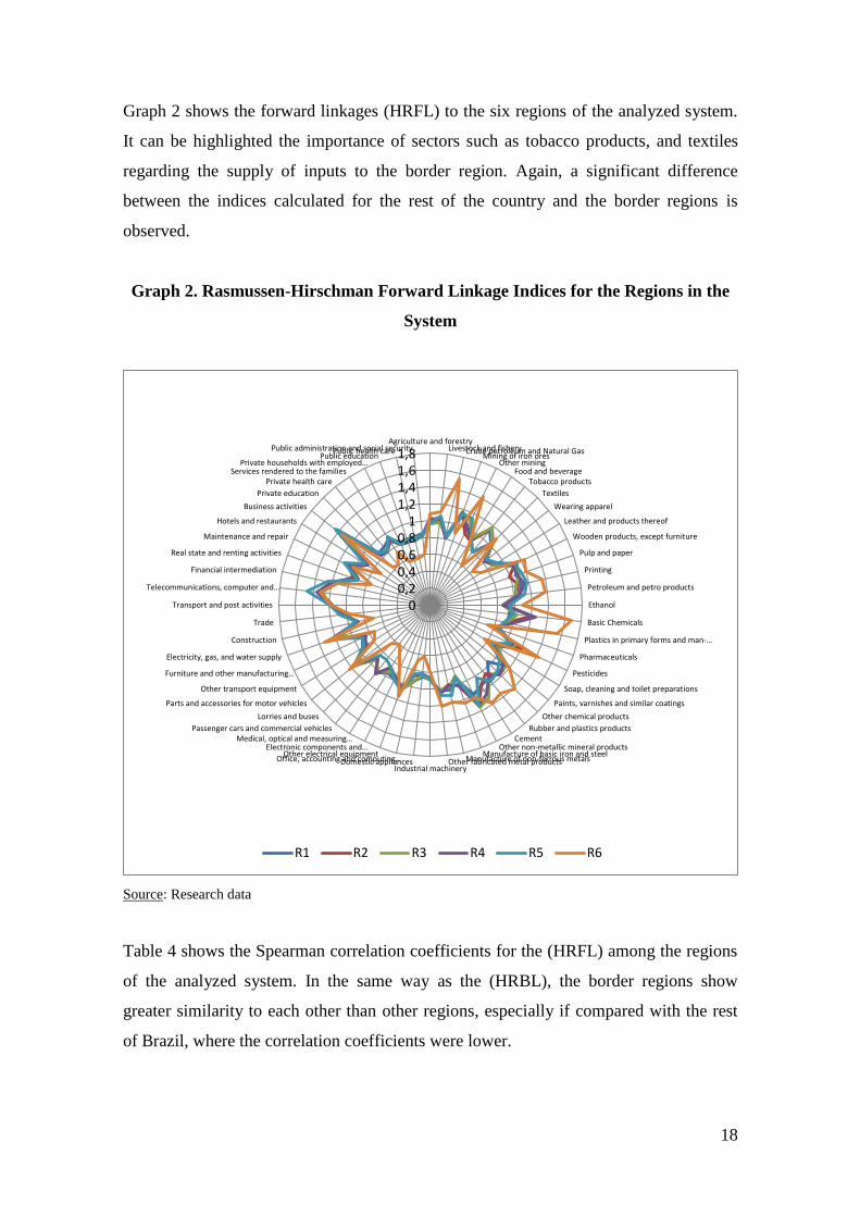
Graph 2 shows the forward linkages (HRFL) to the six regions of the analyzed system.

It can be highlighted the importance of sectors such as tobacco products, and textiles

regarding the supply of inputs to the border region. Again, a significant difference

between the indices calculated for the rest of the country and the border regions is

observed.

Graph 2. Rasmussen-Hirschman Forward Linkage Indices for the Regions in the

System


Table 4 shows the Spearman correlation coefficients for the (HRFL) among the regions

of the analyzed system. In the same way as the (HRBL), the border regions show

greater similarity to each other than other regions, especially if compared with the rest

of Brazil, where the correlation coefficients were lower.

00,20,40,60,8

11,21,41,61,8

Agriculture and forestryLivestock and fisheryCrude petroleum and Natural Gas

Mining of iron oresOther mining


Textiles

Wearing apparel



Pulp and paper

Printing


Ethanol

Basic Chemicals

Plastics in primary forms and man-…

Pharmaceuticals

Pesticides

Soap, cleaning and toilet preparations

Paints, varnishes and similar coatings

Other chemical products

Rubber and plastics productsCement

Other non-metallic mineral productsManufacture of basic iron and steel

Manufacture of non-ferrous metalsOther fabricated metal productsIndustrial machinery

Domestic appliancesOffice, accounting and computing…Other electrical equipment

Electronic components and…Medical, optical and measuring…

Passenger cars and commercial vehicles

Lorries and buses

Parts and accessories for motor vehicles


Furniture and other manufacturing…


Construction

Trade


Telecommunications, computer and…





Business activities

Private education

Private health careServices rendered to the families

Private households with employed…Public education

Public health carePublic administration and social security

R1 R2 R3 R4 R5 R6

19

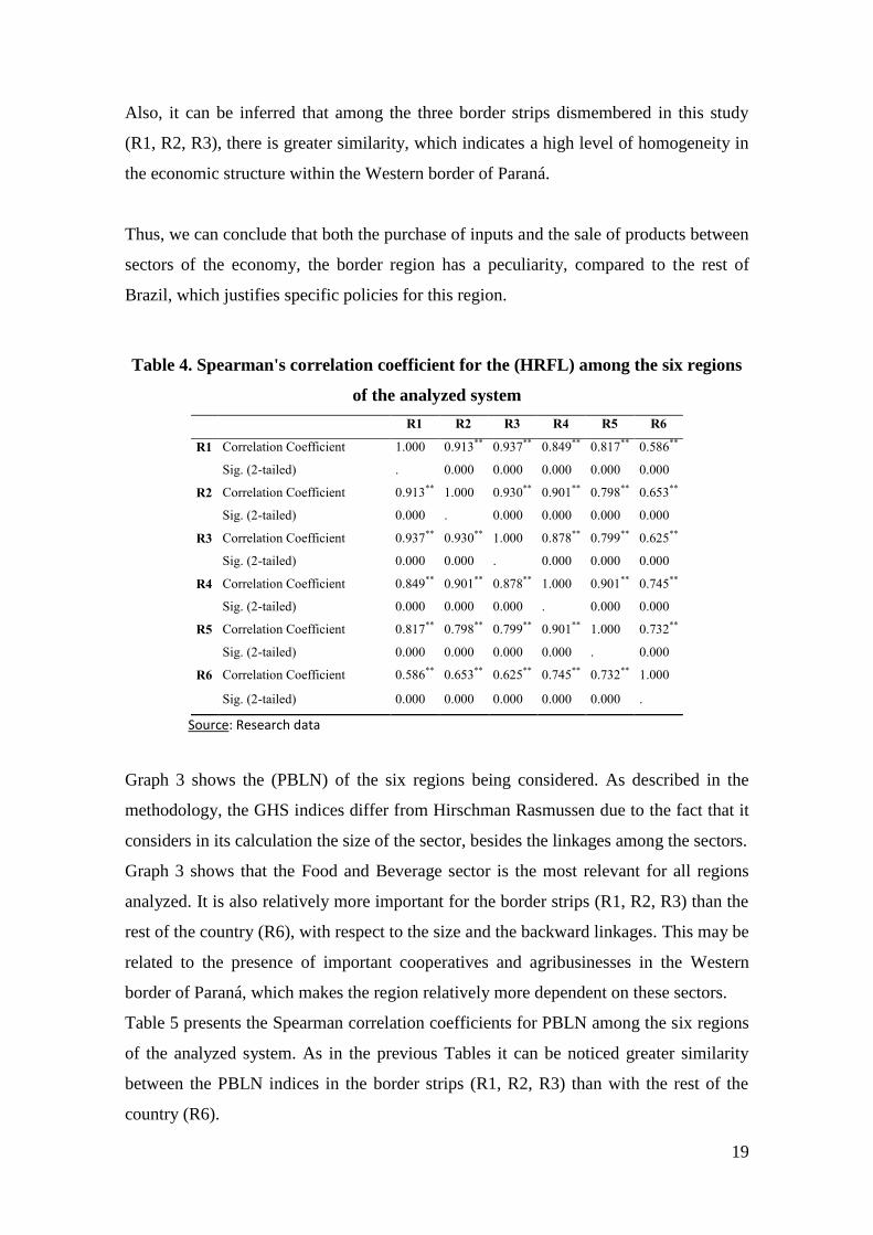
Also, it can be inferred that among the three border strips dismembered in this study

(R1, R2, R3), there is greater similarity, which indicates a high level of homogeneity in

the economic structure within the Western border of Paraná.

Thus, we can conclude that both the purchase of inputs and the sale of products between

sectors of the economy, the border region has a peculiarity, compared to the rest of

Brazil, which justifies specific policies for this region.

Table 4. Spearman's correlation coefficient for the (HRFL) among the six regions

of the analyzed system

R1 R2 R3 R4 R5 R6

R1 Correlation Coefficient 1.000 0.913** 0.937** 0.849** 0.817** 0.586**

Sig. (2-tailed) . 0.000 0.000 0.000 0.000 0.000


Sig. (2-tailed) 0.000 . 0.000 0.000 0.000 0.000


Sig. (2-tailed) 0.000 0.000 . 0.000 0.000 0.000

R4 Correlation Coefficient 0.849** 0.901** 0.878** 1.000 0.901** 0.745**

Sig. (2-tailed) 0.000 0.000 0.000 . 0.000 0.000

R5 Correlation Coefficient 0.817** 0.798** 0.799** 0.901** 1.000 0.732**

Sig. (2-tailed) 0.000 0.000 0.000 0.000 . 0.000

R6 Correlation Coefficient 0.586** 0.653** 0.625** 0.745** 0.732** 1.000

Sig. (2-tailed) 0.000 0.000 0.000 0.000 0.000 .


Graph 3 shows the (PBLN) of the six regions being considered. As described in the

methodology, the GHS indices differ from Hirschman Rasmussen due to the fact that it

considers in its calculation the size of the sector, besides the linkages among the sectors.

Graph 3 shows that the Food and Beverage sector is the most relevant for all regions

analyzed. It is also relatively more important for the border strips (R1, R2, R3) than the

rest of the country (R6), with respect to the size and the backward linkages. This may be

related to the presence of important cooperatives and agribusinesses in the Western

border of Paraná, which makes the region relatively more dependent on these sectors.

Table 5 presents the Spearman correlation coefficients for PBLN among the six regions

of the analyzed system. As in the previous Tables it can be noticed greater similarity

between the PBLN indices in the border strips (R1, R2, R3) than with the rest of the

country (R6).

20

Graph 3: PBLN to the six regions of the analyzed system


Table 5. Spearman's correlation coefficient for the PBLN among the six regions of

the analyzed system

R1 R2 R3 R4 R5 R6


Sig. (2-tailed) . 0.000 0.000 0.000 0.000 0.000


Sig. (2-tailed) 0.000 . 0.000 0.000 0.000 0.000


Sig. (2-tailed) 0.000 0.000 . 0.000 0.001 0.000


Sig. (2-tailed) 0.000 0.000 0.000 . 0.000 0.000


Sig. (2-tailed) 0.000 0.000 0.001 0.000 . 0.000


Sig. (2-tailed) 0.000 0.000 0.000 0.000 0.000 .


02468

101214161820

Agriculture and forestryLivestock and fisheryCrude petroleum and Natural Gas

Mining of iron oresOther mining


Textiles

Wearing apparel



Pulp and paper

Printing


Ethanol

Basic Chemicals

Plastics in primary forms and man-…

Pharmaceuticals

Pesticides

Soap, cleaning and toilet preparations

Paints, varnishes and similar coatings



Other non-metallic mineral productsManufacture of basic iron and steel




Passenger cars and commercial vehicles

Lorries and buses

Parts and accessories for motor vehicles


Furniture and other manufacturing…


Construction

Trade


Telecommunications, computer and…





Business activities

Private education


Private households with employed…Public education

Public health carePublic administration and social security

R1 R2 R3 R4 R5 R6

21

Graph 4 shows the PFLN to the six regions of the interregional system, again we see the

importance of the sectors: a) Agriculture and Forestry; b) Trade; and c) Food and

Beverage sectors for the border. The mentioned sectors are also important for the rest of

the country, but in a lower proportion than for the border strips.

Table 6 presents the Spearman correlation coefficient for the PFLN among the six

regions of the analyzed system. It emphasizes the highest values for the coefficients

among the border strips, indicating greater similarity between the economic structure of

this region, and structural differences with the rest of Brazil, as in the previous tables.

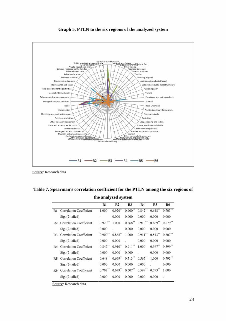
With respect to the PTLN, it can be seen that the sectors of: a) Agriculture and forestry;

b) Livestock and fishery; and c) Food and beverage, are the most important to the

border strips, and in proportional terms are more relevant to the border strips than the

rest of the country, reinforcing the idea of the dependence of the area of traditional

sectors, such as aforementioned. It is shown in Graph 5.

Table 7 presents the Spearman correlation coefficient for the PTLN among the six

regions of the analyzed system. The findings confirm what happens in the previous

tables, reinforcing the homogeneity of the economic structure in the Western border of

Paraná and also its difference from the rest of Brazil as a whole.

22

Graph 4. PFLN to the six regions of the analyzed system


Table 6. Spearman's correlation coefficient for the PFLN among the six regions of

the analyzed system

R1 R2 R3 R4 R5 R6


Sig. (2-tailed) . 0.000 0.000 0.000 .000 0.000


Sig. (2-tailed) 0.000 . 0.000 0.000 0.000 0.000


Sig. (2-tailed) 0.000 0.000 . 0.000 0.000 0.000


Sig. (2-tailed) 0.000 0.000 0.000 . 0.000 0.000


Sig. (2-tailed) 0.000 0.000 0.000 0.000 . 0.000


Sig. (2-tailed) 0.000 0.000 0.000 0.000 0.000 .

Source: Research data.

0

2

4

6

8

10

12Agriculture and forestry

Livestock and fisheryCrude petroleum and Natural GasMining of iron ores

Other miningFood and beverage

Tobacco products

Textiles

Wearing apparel



Pulp and paper

Printing


Ethanol

Basic Chemicals


Pharmaceuticals

Pesticides





Other non-metallic mineral…Manufacture of basic iron and…




Passenger cars and commercial…

Lorries and buses





Construction

Trade







Business activities

Private education


Private households with…Public education

Public health carePublic administration and social…

R1 R2 R3 R4 R5 R6

23

Graph 5. PTLN to the six regions of the analyzed system


Table 7. Spearman's correlation coefficient for the PTLN among the six regions of

the analyzed system

R1 R2 R3 R4 R5 R6


Sig. (2-tailed) . 0.000 0.000 0.000 0.000 0.000


Sig. (2-tailed) 0.000 . 0.000 0.000 0.000 0.000


Sig. (2-tailed) 0.000 0.000 . 0.000 0.000 0.000


Sig. (2-tailed) 0.000 0.000 0.000 . 0.000 0.000


Sig. (2-tailed) 0.000 0.000 0.000 0.000 . 0.000


Sig. (2-tailed) 0.000 0.000 0.000 0.000 0.000 .


0

2

4

6

8

10

12Agriculture and forestry

Livestock and fisheryCrude petroleum and Natural GasMining of iron ores

Other miningFood and beverage

Tobacco products

Textiles

Wearing apparel



Pulp and paper

Printing


Ethanol

Basic Chemicals


Pharmaceuticals

Pesticides





Other non-metallic mineral…Manufacture of basic iron and…




Passenger cars and commercial…

Lorries and buses





Construction

Trade







Business activities

Private education


Private households with…Public education

Public health carePublic administration and social…

R1 R2 R3 R4 R5 R6

24

As described in the database section, the Western border region of Paraná, in this study,

was divided into three groups in order to identify the similarities of internal productive

structure in the region. The results show that there are similarities between the

productive structures in the three specific border strips, highlighting the dependence of

traditional sectors like Food and beverage, Livestock and fishery, and Agriculture and

forestry. Moreover, we also show that the economic structure of the Western Border

Regions of Paraná presents no great similarity with the rest of Brazil as a whole, which

reinforces the need for specific policies to stimulate the growth in the region.

The next section will approach how the interdependence relations of the Western Border

of Paraná are established with itself, the rest of Paraná, Brazil and the rest of the world.

6.2. Interdependence Relations in Output, Employment and Value Added, Among

the Analyzed Regions

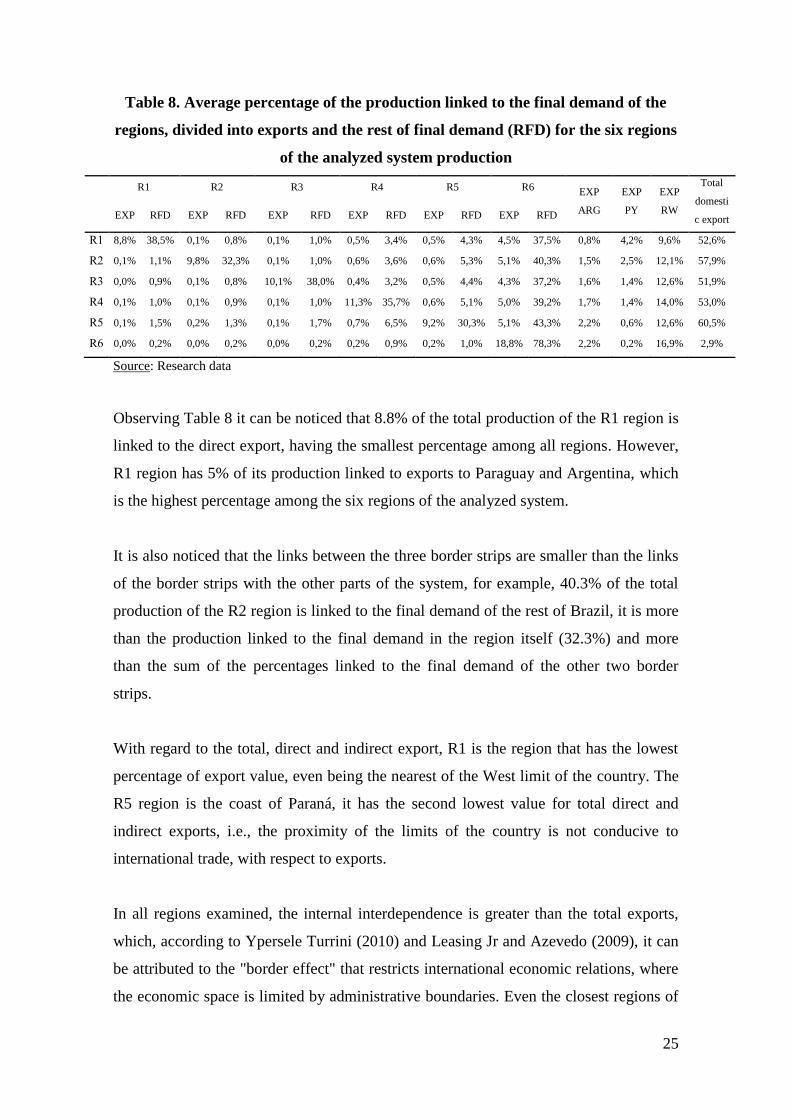
Table 8 shows the trade flows between the six regions of the analyzed system and it is

presented as follows: the first row shows the percentage of total production of the R1

region that is linked to the final demand of itself and all other regions (R2, R3, R4, R5

and R6), divided into inputs for export and domestic production.

The export to Paraguay (EXP PY), to Argentina (EXP ARG) and the rest of the world

(EXP RW) columns present the total production of the each region that is linked to

exports to each one these countries and the rest of the world. And the last column shows

the total domestic exports, i.e., the total production of each region linked to final

demand in other regions of the analyzed system, whether to internal demand or to

exportation.

25

Table 8. Average percentage of the production linked to the final demand of the

regions, divided into exports and the rest of final demand (RFD) for the six regions

of the analyzed system production

R1 R2 R3 R4 R5 R6 EXP

ARG

EXP

PY

EXP

RW

Total

domesti

c export EXP RFD EXP RFD EXP RFD EXP RFD EXP RFD EXP RFD

R1 8,8% 38,5% 0,1% 0,8% 0,1% 1,0% 0,5% 3,4% 0,5% 4,3% 4,5% 37,5% 0,8% 4,2% 9,6% 52,6%

R2 0,1% 1,1% 9,8% 32,3% 0,1% 1,0% 0,6% 3,6% 0,6% 5,3% 5,1% 40,3% 1,5% 2,5% 12,1% 57,9%

R3 0,0% 0,9% 0,1% 0,8% 10,1% 38,0% 0,4% 3,2% 0,5% 4,4% 4,3% 37,2% 1,6% 1,4% 12,6% 51,9%

R4 0,1% 1,0% 0,1% 0,9% 0,1% 1,0% 11,3% 35,7% 0,6% 5,1% 5,0% 39,2% 1,7% 1,4% 14,0% 53,0%

R5 0,1% 1,5% 0,2% 1,3% 0,1% 1,7% 0,7% 6,5% 9,2% 30,3% 5,1% 43,3% 2,2% 0,6% 12,6% 60,5%

R6 0,0% 0,2% 0,0% 0,2% 0,0% 0,2% 0,2% 0,9% 0,2% 1,0% 18,8% 78,3% 2,2% 0,2% 16,9% 2,9%


Observing Table 8 it can be noticed that 8.8% of the total production of the R1 region is

linked to the direct export, having the smallest percentage among all regions. However,

R1 region has 5% of its production linked to exports to Paraguay and Argentina, which

is the highest percentage among the six regions of the analyzed system.

It is also noticed that the links between the three border strips are smaller than the links

of the border strips with the other parts of the system, for example, 40.3% of the total

production of the R2 region is linked to the final demand of the rest of Brazil, it is more

than the production linked to the final demand in the region itself (32.3%) and more

than the sum of the percentages linked to the final demand of the other two border

strips.

With regard to the total, direct and indirect export, R1 is the region that has the lowest

percentage of export value, even being the nearest of the West limit of the country. The

R5 region is the coast of Paraná, it has the second lowest value for total direct and

indirect exports, i.e., the proximity of the limits of the country is not conducive to

international trade, with respect to exports.

In all regions examined, the internal interdependence is greater than the total exports,

which, according to Ypersele Turrini (2010) and Leasing Jr and Azevedo (2009), it can

be attributed to the "border effect" that restricts international economic relations, where

the economic space is limited by administrative boundaries. Even the closest regions of

26

the country limit, both the West and the East, have internal trade flows at least three

times larger than the international transactions.

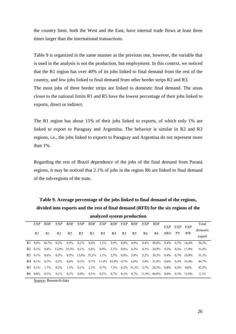
Table 9 is organized in the same manner as the previous one, however, the variable that

is used in the analysis is not the production, but employment. In this context, we noticed

that the R1 region has over 40% of its jobs linked to final demand from the rest of the

country, and few jobs linked to final demand from other border strips R2 and R3.

The most jobs of three border strips are linked to domestic final demand. The areas

closer to the national limits R1 and R5 have the lowest percentage of their jobs linked to

exports, direct or indirect.

The R1 region has about 15% of their jobs linked to exports, of which only 1% are

linked to export to Paraguay and Argentina. The behavior is similar in R2 and R3

regions, i.e., the jobs linked to exports to Paraguay and Argentina do not represent more

than 1%.

Regarding the rest of Brazil dependence of the jobs of the final demand from Paraná

regions, it may be noticed that 2.1% of jobs in the region R6 are linked to final demand

of the sub-regions of the state.

Table 9. Average percentage of the jobs linked to final demand of the regions,

divided into exports and the rest of final demand (RFD) for the six regions of the

analyzed system production

EXP RDF EXP RDF EXP RDF EXP RDF EXP RDF EXP RDF EXP

ARG

EXP

PY

EXP

RW

Total

domestic

export R1 R1 R2 R2 R3 R3 R4 R4 R5 R5 R6 R6

R1 9,0% 34,7% 0,2% 0,5% 0,1% 0,6% 1,1% 2,9% 0,8% 4,9% 4,4% 40,8% 0,4% 0,7% 14,4% 56,3%

R2 0,1% 0,8% 12,9% 35,5% 0,1% 0,6% 0,9% 2,7% 0,8% 6,5% 4,3% 34,9% 0,5% 0,5% 17,9% 51,6%

R3 0,1% 0,6% 0,3% 0,5% 13,6% 35,3% 1,1% 2,5% 0,8% 5,8% 5,2% 34,3% 0,4% 0,7% 19,9% 51,1%

R4 0,1% 0,7% 0,2% 0,6% 0,1% 0,7% 11,4% 43,9% 0,7% 6,0% 3,8% 31,8% 0,6% 0,3% 15,4% 44,7%

R5 0,1% 1,7% 0,2% 1,3% 0,1% 2,1% 0,7% 7,3% 6,2% 51,3% 2,7% 26,3% 0,8% 0,2% 9,0% 42,5%

R6 0,0% 0,1% 0,1% 0,1% 0,0% 0,1% 0,2% 0,7% 0,1% 0,7% 11,9% 86,0% 0,6% 0,1% 11,6% 2,1%


27

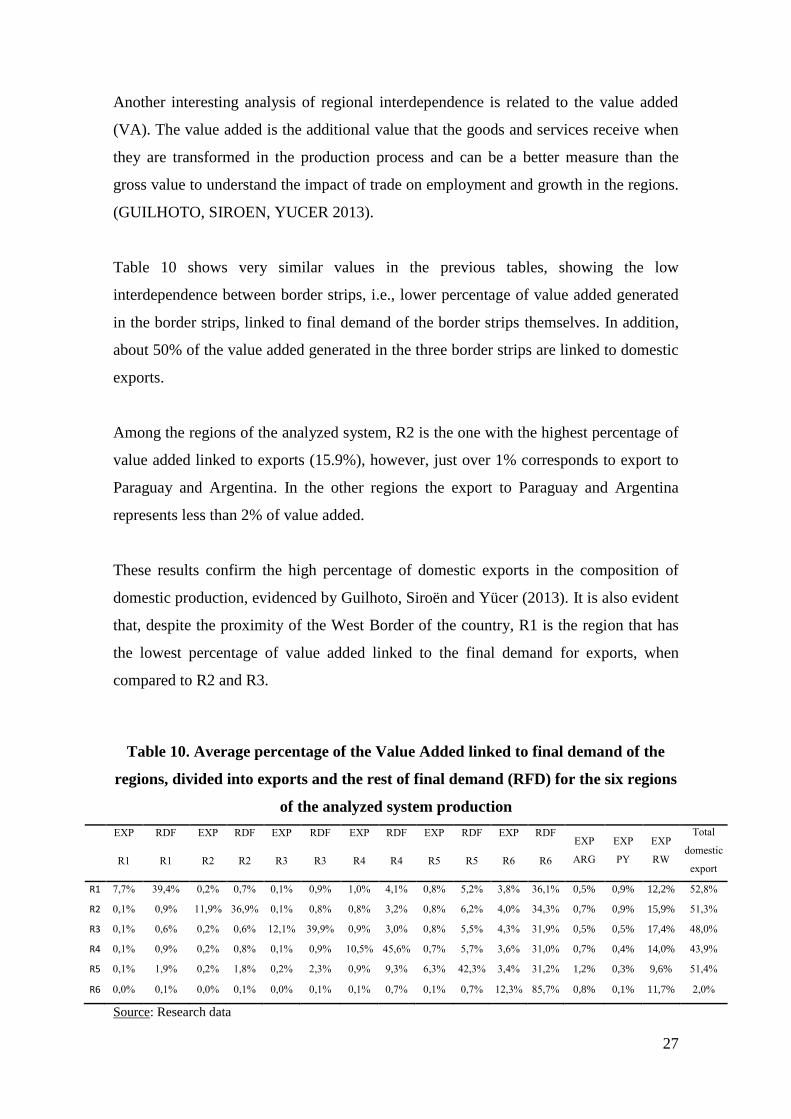
Another interesting analysis of regional interdependence is related to the value added

(VA). The value added is the additional value that the goods and services receive when

they are transformed in the production process and can be a better measure than the

gross value to understand the impact of trade on employment and growth in the regions.

(GUILHOTO, SIROEN, YUCER 2013).

Table 10 shows very similar values in the previous tables, showing the low

interdependence between border strips, i.e., lower percentage of value added generated

in the border strips, linked to final demand of the border strips themselves. In addition,

about 50% of the value added generated in the three border strips are linked to domestic

exports.

Among the regions of the analyzed system, R2 is the one with the highest percentage of

value added linked to exports (15.9%), however, just over 1% corresponds to export to

Paraguay and Argentina. In the other regions the export to Paraguay and Argentina

represents less than 2% of value added.

These results confirm the high percentage of domestic exports in the composition of

domestic production, evidenced by Guilhoto, Siroën and Yücer (2013). It is also evident

that, despite the proximity of the West Border of the country, R1 is the region that has

the lowest percentage of value added linked to the final demand for exports, when

compared to R2 and R3.

Table 10. Average percentage of the Value Added linked to final demand of the

regions, divided into exports and the rest of final demand (RFD) for the six regions

of the analyzed system production

EXP RDF EXP RDF EXP RDF EXP RDF EXP RDF EXP RDF EXP

ARG

EXP

PY

EXP

RW

Total

domestic

export R1 R1 R2 R2 R3 R3 R4 R4 R5 R5 R6 R6

R1 7,7% 39,4% 0,2% 0,7% 0,1% 0,9% 1,0% 4,1% 0,8% 5,2% 3,8% 36,1% 0,5% 0,9% 12,2% 52,8%

R2 0,1% 0,9% 11,9% 36,9% 0,1% 0,8% 0,8% 3,2% 0,8% 6,2% 4,0% 34,3% 0,7% 0,9% 15,9% 51,3%

R3 0,1% 0,6% 0,2% 0,6% 12,1% 39,9% 0,9% 3,0% 0,8% 5,5% 4,3% 31,9% 0,5% 0,5% 17,4% 48,0%

R4 0,1% 0,9% 0,2% 0,8% 0,1% 0,9% 10,5% 45,6% 0,7% 5,7% 3,6% 31,0% 0,7% 0,4% 14,0% 43,9%

R5 0,1% 1,9% 0,2% 1,8% 0,2% 2,3% 0,9% 9,3% 6,3% 42,3% 3,4% 31,2% 1,2% 0,3% 9,6% 51,4%

R6 0,0% 0,1% 0,0% 0,1% 0,0% 0,1% 0,1% 0,7% 0,1% 0,7% 12,3% 85,7% 0,8% 0,1% 11,7% 2,0%


28

6.3. Output Multipliers and Spillover Effects

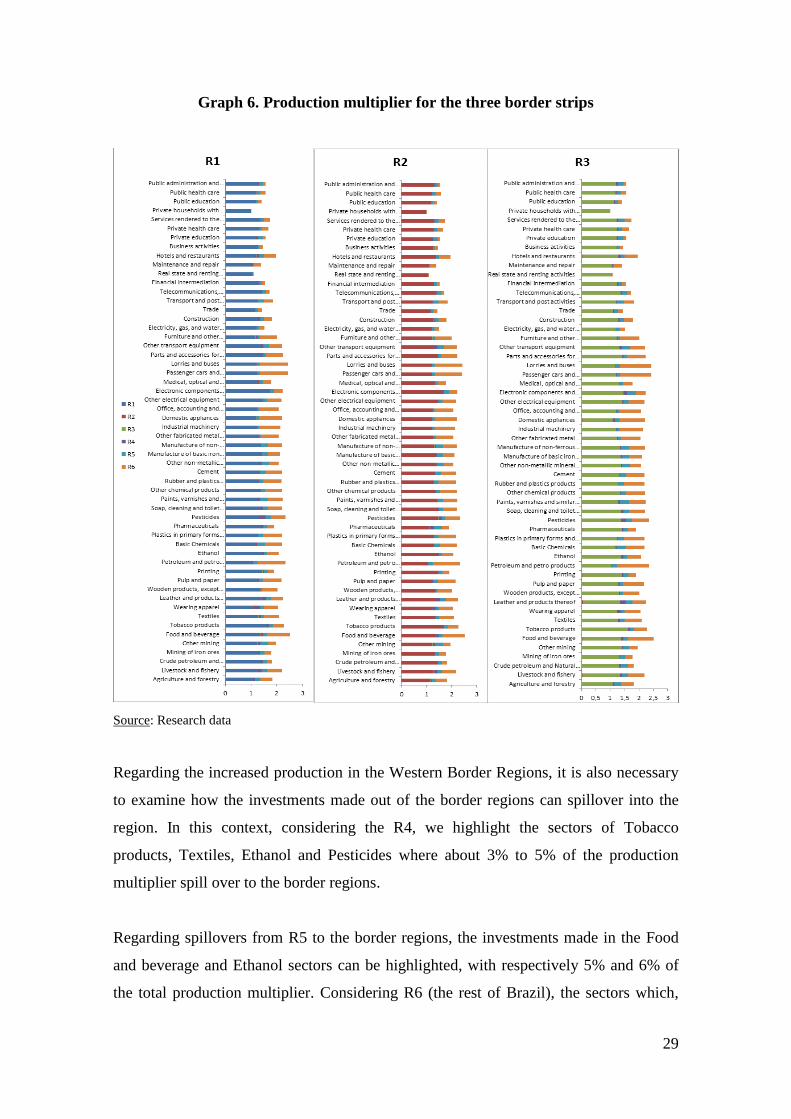
The sector with the largest output multiplier in R1 is the Food and beverage. For each

R$1 of impact on final demand of this sector increases the production in R$ 2.5

throughout the interregional system, however, much of this impact is outside of the R1,

only 53%, i.e., R$ 1.3 remains in the region. There is a spillover effect, mainly to R6

(the rest of Brazil).

Other sectors with high values for the production multiplier in R1 are: Lorries and

buses, Passenger cars and Commercial vehicles and Pesticides, however, all of them

with a low percentage multiplier that really remains in the Region.

Considering the impact within the region of analysis, the sectors with the largest intra-

regional percentage impact are: electronic components and communication equipments,

tobacco products and parts and accessories for motor vehicles, respectively, as shown in

Graph 6.

In R2, the sectors with the highest production multipliers do not generate the highest

percentage of intra-regional impact as in R1. The Food and beverage sector has the

highest production multiplier, considering the whole inter-regional system, but it is the

fifteenth in terms of impact within the region. The sector in which a stimulus in final

demand causes the greatest impact on intra-regional production in R2 is the Tobacco

product.

The sectors with higher percentage on intra-regional production multiplier in R3 are

respectively Tobacco products, Electronic components and Communication equipment,

Parts and accessories for motor vehicles, Other electrical equipment and

Pharmaceuticals.

The pharmaceutical sector is noteworthy since it is the thirty-sixth in the ranking of

production multipliers of R3, but considering the percentage of intra-regional impact,

rises to fifth place (this due to the presence of a large pharmaceutical company in the

R3).

29

Graph 6. Production multiplier for the three border strips


Regarding the increased production in the Western Border Regions, it is also necessary

to examine how the investments made out of the border regions can spillover into the

region. In this context, considering the R4, we highlight the sectors of Tobacco

products, Textiles, Ethanol and Pesticides where about 3% to 5% of the production

multiplier spill over to the border regions.

Regarding spillovers from R5 to the border regions, the investments made in the Food

and beverage and Ethanol sectors can be highlighted, with respectively 5% and 6% of

the total production multiplier. Considering R6 (the rest of Brazil), the sectors which,

30

when stimulated, contribute most to the border regions are Food and beverages and

Tobacco products.

The analysis of production multipliers in border regions makes it possible to observe

that some sectors with high multiplier, as the food and beverage, has its spillover effect

to other regions, other than the border region, and the same sector, when stimulated in

other regions also spills into the border region, but to a lesser extent.

This can be attributed to the fact that the Border Region is a major producer of food

(maize, chicken and pork), however, much of the production is transported to other

regions with little value added. Moreover, most of the inputs used for food production

in the Border Region are imported from other regions.

7. Concluding Remarks

The aim of this study was to analyze the productive structure, national and international

trade relations, besides the spillover of production in the Western Border of Paraná.

It could be noticed that the Western border strips of Paraná (R1, R2, R3) are similar to

each other and different from the rest of Brazil, regarding the productive structure, as

shown in the Spearman correlation coefficient. Moreover, they are more dependent on

traditional sectors of the economy as Food and beverage and Agriculture and Livestock

than the rest of Brazil as a whole.

The results show the low interdependence in respect to production, employment and

value added between the border regions, and a greater relationship with the rest of

Brazil, this can be explained by the homogeneity of the productive structure between the

border regions, which make the complementary relationship between economic sectors

difficult and does not promote the trade between regions.

The R1 region has 8.8% of its production linked to direct export, more than a half of

this value, about 5%, is linked to exports to Paraguay and Argentina. It is the highest

percentage among all regions analyzed, but not sufficient to put R1 among the main

exporters. The proximity of both West and East borders of the country does not increase

31

exports of R1 and R5 regions enough to excel them as exporters. It can be a result of the

"border effect", as described in literature.

It may suggest that the proximity of the limits is not considered strategic for export

companies to choose locations in the border region. There are other factors determining

the location of these companies, apart from the distance to markets.

Analyzing the output multipliers and the spillover effects to outside of the region, it was

noticed that the Food and beverage sector has the major output multiplier for the three

border strips, but only a portion of this multiplier remains in the original regions,

approximately half of the production multiplier spills over out of the border regions.

Moreover, the strong dependence of the border region from traditional sectors of the

economy exacerbates the spillover effect, for example in agriculture and forestry and

livestock sectors, only about 60% and 56% of the effect remains in the region,

respectively.

In conclusion, it is suggested that regional policy makers invest in public policies that

promote the complementarity of the production chain, increasing the processing of the

products within the border region, and thus increasing the multiplier effect of the

production within the region. Besides, increasing the interdependence between the

border regions and stimulating "fluency effect" and consequently, increasing the

number of jobs and value added generated within that region.

It should be emphasized that the results presented in this study are specific to the

Western Border Regions of Paraná State, given its peculiarities and idiosyncrasies, it is

not possible to generalize to other regions. Therefore, we emphasize the importance of

interregional input-output studies, which allow the structural analysis of regions and

their interdependencies, in order to enable the definition of development strategies that

are better suited for each region.

32

References

ANDRADE, T. A. Desigualdades Regionais no Brasil: Uma Seleção de Estudos

Empíricos. In: SCHWARTZMAN, J., Economia Regional. Belo Horizonte,

Cedeplar, 1977.

BAUMOL W. J.; WOLFF E. N. A key role for input-output analysis in policy design.

Regional Science and Urban Economics. n. 24; 1994, p. 93-113.

GUILHOTO, J. J. M. Análise de Insumo-Produto: Teoria e Fundamentos. São

Paulo: FEA-USP, disponível <em: http://mpra.ub.uni-

muenchen.de/32566/2/MPRA_paper_32566.pdf>, 2011. 64p.

GUILHOTO, J. J. M.; AZZONI, C. R.; ICHIHARA, S. M.; KADOTA, D. K.;

HADDAD, E.A. Matriz de Insumo-Produto do Nordeste e Estados. Fortaleza:

Banco do Nordeste do Brasil. Disponível em: <

http://www.usp.br/nereus/?fontes=dados-matrizes>. Acesso em: 08 jun. 2013

GUILHOTO, J.J.M.; SONIS, M.; HEWINGS, G.J.D. Linkages and Multipliers in a

Multiregional Framework: Integration of Alternative Approaches. Australasian

Journal of Regional Studies, v.11, n.1, pp. 75-89, 2005.

HIRSCHMAN, A.O. The Strategy of Economic Development. Yale University Press,

1958.

HIRSCHMAN, A. Transmissão Inter-regional e Internacional do Crescimento

Econômico. In: SCHWARTZMAN, J., Economia Regional. Belo Horizonte,

Cedeplar, 1977.

HISSA, C. E. V. A mobilidade das fronteiras: inserções da geografia na crise da

modernidade. Editora UFMG. Belo Horizonte, 2002. 316p.

HOLMES, T.J.; STEVENS J.J. Exports, borders, distance and plant size. Journal of

International Economics, v 88, Issue 1, 2012, p 91-103.

INSTITUTO BRASILEIRO DE GEOGRAFIA E ESTATÍSTICA (IBGE), disponível

em <www.ibge.gov.br>. acesso em 15 de julho de 2013.

INSTITUTO PARANAENSE DE DESENVOLVIMENTO ECONÔMICO E SOCIAL

(IPARDES). Anuário Estatístico do Estado do Paraná. Disponível em:

<http://www.ipardes.gov.br/anuario_2006/index.html>. Acesso em: 03 julho. 2013.

LEONTIEF, W. The Structure of the American Economy. Oxford University Press,

1951.

http://mpra.ub.uni-muenchen.de/32566/2/MPRA_

http://mpra.ub.uni-muenchen.de/32566/2/MPRA_

http://www.ibge.gov.br/

33

LEUSIN JR., S. ; AZEVEDO, A. F. Z. . O Efeito Fronteira das Regiões Brasileiras:

Uma Aplicação do Modelo Gravitacional. Revista de Economia Contemporânea,

v. 13, 2009, p. 229-258.

MILLER, R.E.;BLAIR, P.D. Input-output analysis: foundations and extensions.

Prentice Hall Inc., New Jersey. 2009.

MORSHED, M.A.K.M, What can we learn from a large border effect in

developing countries? Journal of Development Economics, V.72, Issue 1,

October 2003, P 353-369.

PARSLEY, D. C.; WEI, S. J. Expaining the border effect: the role of exchange rate

variability, shipping costs, and geography. Journal of International Economics.

n.55, 2001, p. 87-105.

PORTES, R.; REY, H. The determinants of cross-border equity flows. Journal of

International Economics, v. 65, Issue 2, 2005, p. 269-296.

RASMUSSEN, P. Studies in Intersectoral Relations, North Holland, 1956.

ROLIM, C. Como Analisar as Regiões Fronteiriças: Esboço de um Enquadramento

Teórico-Metodológico a partir do caso de Foz do Iguaçu. Anais III Encontro de

Economia Paranaense. Londrina 2004.

SONIS, M.; HEWINGS, G. J D.; GUO J.; HULU E. Interpreting spatial economic

structure: feedback loops in the Indonesian interregional economiy, 1980, 1985.

Regional Science and Uban Economics. n. 27, 1997, p. 325-342.

SOUZA, E. B. C.; GEMELLI, V. Território, Região e Fronteira: Análise Geográfica

Integrada da Fronteira Brasil/Paraguai. Revista Brasileira de Estudos Urbanos e

Regionais, v13, n2. Novembro, 2011.

SOUZA, J. S. Teoria dos polos, regiões inteligentes e sistemas regionais de inovação.

Análise, v. 16 n. 1, 2005, p. 87-112.

TURRINI, A. TANGUY, V. Y. Traders, courts, and the border effect puzzle. Regional

Science and Urban Economics. v. 40, 2010, p. 81-91.

WILLIAMSON, J. Desigualdade Regional e o Processo de Desenvolvimento Nacional:

Descrição dos Padrões. In: SCHWARTZMAN, J., Economia Regional. Belo

Horizonte, Cedeplar, 1977.

http://lattes.cnpq.br/4814990938931183

Documents

PRODUCTIVE STRUCTURE AND TRADE RELATIONS: … · Productive Structure and Trade Relations: ... unit shipping cost and fluctuations in exchange rates, ... Acre, Amazonas and Roraima,