Production Lead Time in Serial Lines: Evaluation,Analysis, and Control

Semyon M. Meerkov and Chao-Bo Yan

Department of Electrical Engineering and Computer ScienceUniversity of Michigan, Ann Arbor, MI 48109-2122

Abstract

Production Lead Time (LT ) is the average time a part spends in the system, being processedor waiting for processing. In systems with unlimited buffers, LT may be orders of magnitudelarger than the total processing time, leading to serious economic and quality problems. Atpresent, no systematic analytical methods for evaluation, analysis, and control of LT in sys-tems with machines having up- and downtime characterized by continuous random variablesare available. This paper is intended to develop such methods. Specifically, we address syn-chronous serial lines with exponential machines and derive formulas for LT as a function ofmachine parameters and raw material release rate. Using these formulas, we develop methodsfor open- and closed-loop raw material release, which result in the desired LT . For asyn-chronous exponential lines, we provide an upper bound on LT . For non-exponential lines (e.g.,Weibull, gamma, and log-normal), we offer an empirical formula for LT as an affine functionof the coefficient of variation. The results reported in this paper enable a new paradigm forproduction systems management, namely: manage a production system so that the desired LTis ensured, while the throughput is maximized.

Keywords: Production systems, Lead time, Exponential and non-exponential reliability models,Open- and closed-loop raw material release control.

1 Introduction

1.1 Issues addressed and results obtained

Production Lead Time (LT ) is the average time a part spends in the system, being processed or

waiting for processing. In systems with unlimited buffers, LT may be orders of magnitude larger

than the total processing time, leading to serious economic and quality problems. Unlike other

performance measures, such as throughput (TP), work-in-process (WIP), blockages (BL), and star-

vations (ST ), evaluation and analysis/control of LT received relatively little attention in the current

literature. The goal of this paper is to develop systematic analytical methods for evaluation and

analysis of LT in serial lines with machines having their up- and downtime described by contin-

uous random variables and, using these methods, provide recommendations for LT control and

management.

To accomplish this, first we consider the simplest case – the serial lines with identical expo-

nential machines. This case offers a possibility of detailed analytical investigation of LT and, more

importantly, provides insights into the behavior of LT as a function of machine parameters and raw

material release rate. In addition, it permits the development and investigation of simple open-

and closed-loop raw material release policies, which ensure the desired LT ’s, while maximizing

TP. Then, we extend these results to more practical cases. Specifically, we consider synchronous

exponential lines with non-identical machines and carry out an analytical investigation, similar to

that of the simplest case. Finally, we address asynchronous exponential and non-exponential lines;

for the former, we derive an upper bound on LT , expressed through auxiliary synchronous expo-

nential lines; for the latter, we provide an empirical formula for their LT ’s as a function of up- and

downtime coefficient of variation.

From the mathematical perspective, this work is based on evaluating LT for synchronous se-

rial lines with exponential machines (using the expressions for TP and WIP and Little’s law) and

investigating analytical and structural properties of the resulting expressions. In addition, these

expressions are used to design open- and closed-loop raw material release policies, which ensure

the desired LT .

From the operational perspective, this work is based on associating a raw material release con-

1

trol mechanism with production lines under consideration. Initially, this mechanism is modeled as

an auxiliary exponential machine, leading to random, once-per-cycle, raw material release. Then,

the results are extended to deterministic, e.g., once-per-hour or once-per-shift, release. Finally, for

the case when only nominal values of machine parameters are known and the real ones may differ

from the nominal, we offer a relay-type closed-loop release policy, which is based on the real-time

WIP.

From the managerial perspective, the results of this paper enable a new paradigm of production

management: rather than maximizing TP (which may lead to unlimited LT ), manage the production

systems so that the desired LT is ensured, while TP is maximized.

1.2 Related literature

The current literature on production lead time can be classified into three groups. The first one

considers the lead time as a function of the dispatch, rather than release, rule [1–7]. Dispatch

rules indicate which job must be selected for processing at a given machine or workcenter. The

main result here is that, under a wide range of conditions, jobs with the shortest processing time

should be selected first in order to minimize the lead time. The second, and the most prolific,

group addresses the problem of feedback control of raw material release. The main techniques

considered here are kanban [8–20], CONWIP [21–27], and their comparisons [28–32]. However,

with a few exceptions, this literature does not provide rigorous methods for selecting parameters

of these control strategies (e.g., the numbers of kanbans and CONWIP), which ensure the desired

lead time. A notable exception is a recent article [33], where a method for calculating the smallest

number of kanbans that ensures the desired level of customer service in exponential lines with

finite buffers are provided. The third, and the least copious, group consists of recent publications

on lead time analysis using analytical tools. It includes papers [34–37], where distributions of

lead time are derived for production systems with exponential processing time and Poisson order

arrival. In [38], these results are extended to multi-product systems. An approach to lead time

reduction based on manufacturing intelligence is developed in [39], where neural networks have

been employed to evaluate WIP in a semiconductor manufacturing facility and used subsequently

2

for lead time analysis and control. Finally, [40] considers serial lines with finite buffers and derives

lower bounds on the production completion time, which is closely related to the lead time.

Our initial results on LT evaluation, analysis, and control have been reported in [41] and [42]

for serial and cellular lines, respectively. Both of these papers assume that the machines obey

the Bernoulli reliability model, according to which a machine produces a part during a cycle time

with probability p and fails to do so with probability 1 − p (see [43] for details). While this

reliability model is applicable to assembly operations with downtimes close to the machine cycle

time, it is not applicable to machining and other operations, where the downtime is typically much

longer than the cycle time. Also, the Bernoulli model, being defined by a single parameter, does

not offer a possibility of investigating various qualitative properties of LT , e.g., the effects of up-

and downtime on LT . These shortcomings necessitate the development of methods for evaluation,

analysis, and control of LT in production systems with more practical reliability models, e.g.,

exponential, Weibull, gamma, log-normal, etc. This is carried out in the current paper.

1.3 Paper outline

The outline of this paper is as follows: In Section 2, a model of production systems with a raw

material release mechanism is introduced, and the problems addressed are stated. Sections 3-5

provide a solution of these problems for the simplest case – serial lines with identical exponential

producing machines. As mentioned in Subsection 1.1, this case is considered in details because

it provides clear insights into the lead time behavior and control. In Sections 6 and 7, extensions

to systems with a wider practical applicability are provided. Namely, in Section 6, we report ana-

lytical results on the evaluation, analysis, and control of LT in synchronous exponential lines with

non-identical producing machines. In Section 7, we offer an upper bound on LT in asynchronous

exponential lines and an empirical formula for LT in lines with non-exponential machines. The

conclusions and topics for future research are given in Section 8. The proofs are included in the

Appendix.

3

2 Modeling and Problems Addressed

Consider a serial line shown in Figure 2.1, where the circles represent the machines and the open

rectangles are the buffers. While m1,m2, . . . ,mM and b1, b2, . . . , bM−1 are the usual producing ma-

chines and unlimited work-in-process buffers, respectively, m0 represents the raw material release

machine and b0 unlimited raw material buffer (to indicate this, m0 and b0 are shown in gray). Con-

trolling the efficiency of the release machine, m0, one can control the availability of raw material

in the system and, thus, the lead time.

Figure 2.1: Serial production line with a release machine

To formalize this model, we introduce the following assumptions:

(i) The system consists of M producing machines, m1,m2, . . . ,mM, a release machine, m0, M−1

work-in-process buffers, b1, b2, . . . , bM−1, and a raw material buffer, b0.

(ii) Each machine is characterized by its cycle time, τi (in min), i = 0, 1, . . . , M. If cycle times of

all machines (including the release machine) are identical, the system is called synchronous;

otherwise, it is asynchronous. While in the asynchronous case, τi, i = 1, 2, . . . , M, are fixed,

τ0 is free and can be selected at will.

(iii) In addition, each machine is characterized by its reliability model, i.e., continuous random

variables that define its up- and downtime. If these distributions are exponential, i.e., defined

by the breakdown rate λi and repair rate µi, i = 0, 1, . . . , M, (both in 1/min), the line is called

exponential; otherwise, it is non-exponential. While for the producing machines, λi and µi,

i = 1, 2, . . . , M, are fixed, for the release machine, λ0 and µ0 are design parameters that can

be selected at will.

(iv) Each buffer is of infinite capacity.

4

(v) The flow model [43] is assumed, i.e., infinitesimal quantity of parts, produced during an

infinitesimal time interval, are transferred to and from the buffers. A machine is starved, if

the buffer in front of it is empty; m0 is never starved. Machine failures are time-dependent

[43], i.e., a machine can be down even if it is starved.

Assumption (iv) is introduced to reflect the fact that the lead time control problem is of partic-

ular importance for systems with practically unlimited storage, e.g., with no hardware-constrained

buffers. Assumption (v) is introduced for technical reasons: it permits a precise formulation of the

equations describing the systems at hand (a justification of this assumption is given in [43]).

Let Tup,i and Tdown,i denote the average up- and downtime of the machines, i = 0, 1, . . . , M.

Then the machine efficiency for any continuous reliability model is:

ei :=Tup,i

Tup,i + Tdown,i, i = 0, 1, . . . , M, (2.1)

and its throughput in isolation (i.e., when the machine is not starved) is

TPisol,i :=Tup,i

τi(Tup,i + Tdown,i), i = 0, 1, . . . , M. (2.2)

Since for exponential machines, Tup,i = 1λi

and Tdown,i = 1µi

,

ei =µi

λi + µiand TPisol,i =

µi

τi(λi + µi), i = 0, 1, . . . , M. (2.3)

Clearly, to obtain meaningful results, it should be assumed that e0 < ei, i = 1, 2, . . . , M, for

synchronous lines or TPisol,0 < TPisol,i, i = 1, 2, . . . , M, for asynchronous ones (otherwise, LT is

unbounded).

For the case of finite buffer capacity, an analytical method for evaluating the throughput and

work-in-process in each buffer (WIPi, i = 0, 1, . . . , M) of exponential serial lines is given in [43].

In the current paper, we extend this method to the case of infinite buffers and address the following

problems:

• Derive an analytical expression for LT in synchronous exponential lines as a function of λi

5

and µi, i = 0, 1, . . . , M.

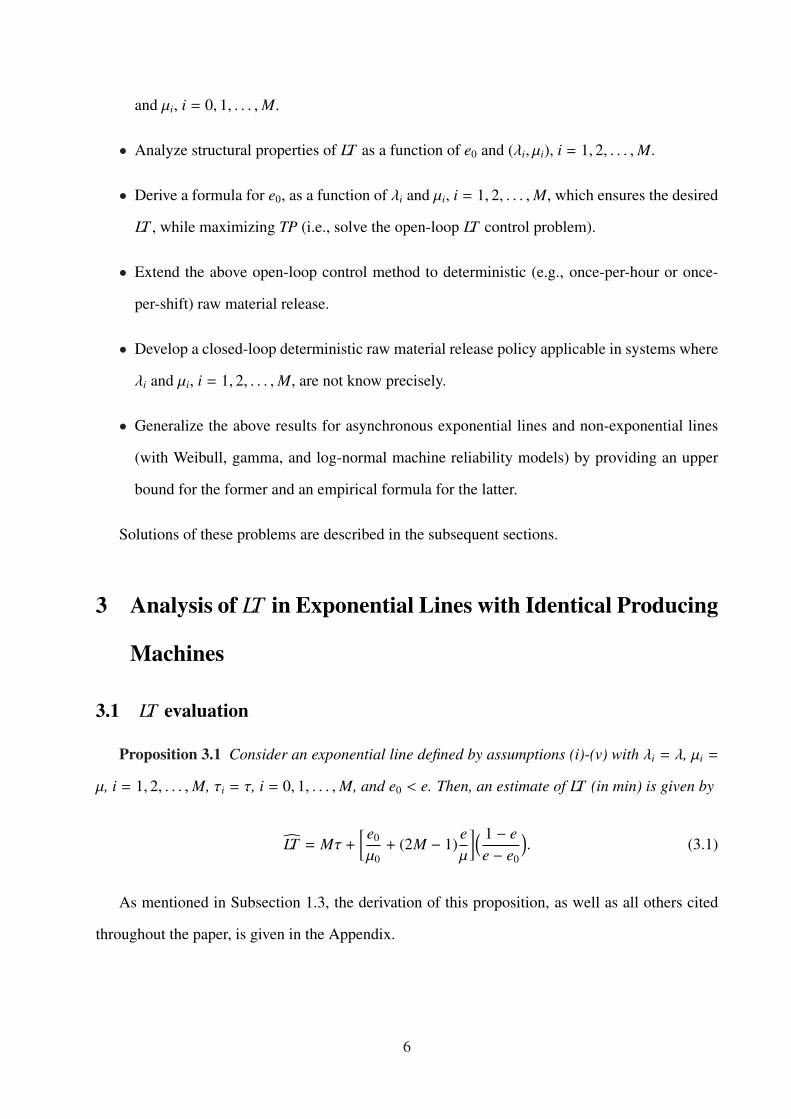
• Analyze structural properties of LT as a function of e0 and (λi, µi), i = 1, 2, . . . , M.

• Derive a formula for e0, as a function of λi and µi, i = 1, 2, . . . , M, which ensures the desired

LT , while maximizing TP (i.e., solve the open-loop LT control problem).

• Extend the above open-loop control method to deterministic (e.g., once-per-hour or once-

per-shift) raw material release.

• Develop a closed-loop deterministic raw material release policy applicable in systems where

λi and µi, i = 1, 2, . . . , M, are not know precisely.

• Generalize the above results for asynchronous exponential lines and non-exponential lines

(with Weibull, gamma, and log-normal machine reliability models) by providing an upper

bound for the former and an empirical formula for the latter.

Solutions of these problems are described in the subsequent sections.

3 Analysis of LT in Exponential Lines with Identical Producing

Machines

3.1 LT evaluation

Proposition 3.1 Consider an exponential line defined by assumptions (i)-(v) with λi = λ, µi =

µ, i = 1, 2, . . . , M, τi = τ, i = 0, 1, . . . , M, and e0 < e. Then, an estimate of LT (in min) is given by

LT = Mτ +

[ e0

µ0+ (2M − 1)

eµ

]( 1 − ee − e0

). (3.1)

As mentioned in Subsection 1.3, the derivation of this proposition, as well as all others cited

throughout the paper, is given in the Appendix.

6

The accuracy of this estimate has been evaluated by simulating exponential lines with parame-

ters M, e, e0, Tdown, and Tdown,0 selected randomly and equiprobably from the following sets:

M ∈ [3, 10], e ∈ [0.7, 0.99], e0 ∈ [0.7e, 0.99e], Tdown ∈ [10min, 100min], Tdown,0 = Tdown. (3.2)

For each line, thus formed, the simulations were carried out for two τ’s: τ = 0.5min and τ = 5min.

The total of 1000 lines have been simulated using the following procedure: For each line, in

addition to a warm-up period of 2, 000, 000min, the simulation was carried out for 22, 000, 000min;

20 repetitions of this procedure were carried out to evaluate LT . This simulation procedure results

in a 95% confidence interval of ±0.87% of LT for both τ = 0.5min and τ = 5min. The accuracy

of (3.1) was quantified by εLT = |LT−LT |LT × 100%. As a result, we obtained: For τ = 0.5min, the

smallest and the largest errors were 0.0025% and 8.97%, respectively, and the average error was

2.17%; for τ = 5min, the smallest and the largest errors were 0.0007% and 7.21%, respectively,

and the average error was 1.99%. Based on these results and recognizing that machine parameters

on the factory floor are rarely known with accuracy better than ±5%, we conclude that estimate

(3.1) is precise enough for the lead time analysis and control.

Expression (3.1) leads to the following:

Observation 3.1 For fixed e and e0, shorter up- and downtimes lead to smaller LT . As e→ 1,

LT tends to its minimum value, Mτ. LT is monotonically increasing in M, hyperbolically increasing

as e0 → e, and is an affine function of τ with the slope M.

To further analyze the behavior of LT , introduce the following parametrization:

ρ :=e0

e, lt :=

LTMτ

. (3.3)

We refer to 0 < ρ < 1 as the relative workload imposed on the system and to lt > 1 as the relative

lead time (dimensionless), i.e., the lead time in units of the smallest possible lead time. In terms of

these parameters, (3.1) becomes

lt = 1 +1τ

(ρ

Mµ0+

2M − 1Mµ

)(1 − e1 − ρ

). (3.4)

7

Clearly, in addition to M, e, and τ, the relative lead time, lt, depends on the release machine

efficiency, e0 (through ρ) and on its downtime (through µ0). However, in the limit as M tends to

infinity, the dependence on µ0 disappears:

lt∞ := limM→∞

lt = 1 +2µτ

(1 − e1 − ρ

). (3.5)

This is important for the lead time control problem, since for sufficiently long lines, only e0 would

need to be selected, rather than µ0 as well. It can be shown that if µ0 > µ, the accuracy of this

approximation in terms of ∆ = lt∞−ltlt∞

is quantified as 0 < ∆ < 12M . Thus, lt∞ > lt, and the error, ∆,

decreases hyperbolically in M. Therefore, (3.5) can be viewed as a relatively tight bound of (3.4).

From (3.5) follows another fact: If µτ = 2e, then (3.5) becomes

lt∞ =e−1 − ρ1 − ρ , (3.6)

which is exactly the same as the expression for lt in Bernoulli serial lines (see [41]), with the

Bernoulli machine efficiency p being substituted by the exponential machine efficiency e. Hence,

from (3.5) and (3.6), follows:

Observation 3.2 If µτ = 2e, then lt∞ in exponential lines equals lt in Bernoulli lines with

p = e. If µτ < 2e, then lt∞ in exponential lines is larger than lt in Bernoulli lines with p = e.

Since µτ < 2e implies that Tdown >τ2 (which is practically always the case), we conclude that lt in

exponential lines is generically larger than lt in Bernoulli lines with p = e.

3.2 Structural properties of lt(ρ)

Figure 3.1 illustrates the behavior of lt given by (3.4) as a function of ρ for M = 10, τ = 1min and

several values of e, µ, and µ0; the Bernoulli case, i.e., when µτ = 2e, is also shown for comparison.

All curves in this figure have a “knee” beyond which lt grows extremely fast. In practice, this

knee is refered to as the “sweet point”, since TP is maximized, while LT remains relatively small.

Therefore, it is important to quantify the position of the knee.

To accomplish this, consider the (ρ, lt)-plane, where a unit interval of ρ-axis corresponds to

8

A > 1 units of lt-axis (in Figure 3.1, A = 4000). Introduce the scaling ratio, α, defined by

α :=1A

(3.7)

and recall that the curvature, κ, of a twice differentiable function, f (x), is given by (see [44])

κ(f (x)

)=

∣∣∣ f ′′xx

∣∣∣(1 + f ′2x )

32

. (3.8)

0.7 0.8 0.9 10

400

800

1200

ρ

lt 0.98 0.99 10

40

80µ0 = 0.01, µ = 0.1

µ0 = 1, µ = 0.1

µ0 = 0.1, µ = 0.01

µ0 = 0.1, µ = 1

Bernoulli

(ρknee, ltknee)(0.880, 479.45)

(0.953, 184.55)(0.962, 152.36)

(0.985, 59.69)

(0.990, 42.40)

(a) e = 0.7

0.7 0.8 0.9 10

400

800

1200

ρ

lt 0.98 0.99 10

40

80

µ0 = 0.01, µ = 0.1

µ0 = 1, µ = 0.1

µ0 = 0.1, µ = 0.01

µ0 = 0.1, µ = 1

Bernoulli

(ρknee, ltknee)

(0.902, 391.70)

(0.962, 151.32)(0.969, 124.59)

(0.988, 48.97)

(0.992, 32.62)

(b) e = 0.8

0.7 0.8 0.9 10

400

800

1200

ρ

lt 0.98 0.99 10

40

80

µ0 = 0.01, µ = 0.1

µ0 = 1, µ = 0.1

µ0 = 0.1, µ = 0.01

µ0 = 0.1, µ = 1

Bernoulli

(ρknee, ltknee)

(0.931, 277.31)

(0.973, 107.70)(0.978, 88.40)

(0.992, 34.96)

(0.995, 22.08)

(c) e = 0.9

Figure 3.1: Relative lead time, lt, as a function of relative workload, ρ, and machine parameters(for M = 10, τ = 1min)

Definition 3.1 The knee, ρknee, of lt on the (ρ, lt)-plane with the scaling ratio α is the point on

[0, 1) at which the curvature of αlt(ρ) reaches its maximum.

Proposition 3.2 Under the assumptions of Proposition 3.1,

ρknee = 1 −√

α

Mτ

( 1µ0

+2M − 1

µ

)(1 − e) (3.9)

and

limM→∞

ρknee = 1 −√

2αµτ

(1 − e). (3.10)

The pairs (ρknee, lt(ρknee)) are indicated in Figure 3.1 by black dots. Thus, releasing raw material

with the rate

e0 < e(1 −

√α

Mτ

( 1µ0

+2M − 1

µ

)(1 − e)

), (3.11)

9

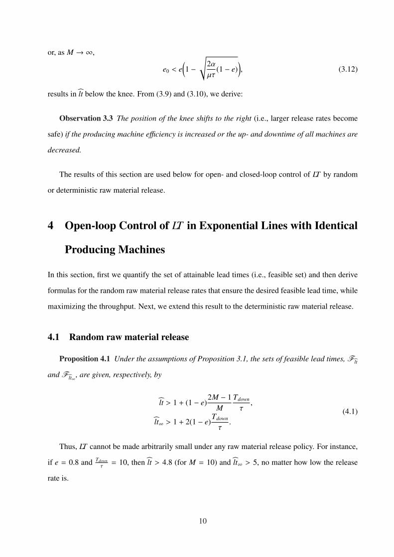
or, as M → ∞,

e0 < e(1 −

√2αµτ

(1 − e)), (3.12)

results in lt below the knee. From (3.9) and (3.10), we derive:

Observation 3.3 The position of the knee shifts to the right (i.e., larger release rates become

safe) if the producing machine efficiency is increased or the up- and downtime of all machines are

decreased.

The results of this section are used below for open- and closed-loop control of LT by random

or deterministic raw material release.

4 Open-loop Control of LT in Exponential Lines with Identical

Producing Machines

In this section, first we quantify the set of attainable lead times (i.e., feasible set) and then derive

formulas for the random raw material release rates that ensure the desired feasible lead time, while

maximizing the throughput. Next, we extend this result to the deterministic raw material release.

4.1 Random raw material release

Proposition 4.1 Under the assumptions of Proposition 3.1, the sets of feasible lead times, Flt

and Flt∞ , are given, respectively, by

lt > 1 + (1 − e)2M − 1

MTdown

τ,

lt∞ > 1 + 2(1 − e)Tdown

τ.

(4.1)

Thus, LT cannot be made arbitrarily small under any raw material release policy. For instance,

if e = 0.8 and Tdownτ

= 10, then lt > 4.8 (for M = 10) and lt∞ > 5, no matter how low the release

rate is.

10

Proposition 4.2 Under the assumptions of Proposition 3.1, for any feasible desired lead time,

ltd ∈ Flt, the release rate is given by

e∗0 = e[1 − µ + (2M − 1)µ0

Mµµ0τ(ltd − 1) + µ(1 − e)(1 − e)

]. (4.2)

For this release rate,

TP∗

=e∗0τ, WIP

∗0 =

e∗0τ

( e∗0µ0

+eµ

)( 1 − ee − e∗0

), WIP

∗i =

2e∗0eµτ

( 1 − ee − e∗0

), i = 1, 2, . . . , M − 1. (4.3)

This proposition leads to a solution of the open-loop lead time control problem based on the

following arguments:

• Since, as it is possible to show, de∗0dµ0

> 0, the throughput TP∗

is maximized as µ0 → ∞. In this

case, the release rate that results in ltd, becomes:

e∗0(µ0 = ∞) := limµ0→∞

e∗0 = e[1 − (2M − 1)(1 − e)

M(ltd − 1)Tdown

τ

]. (4.4)

• Having µ0 → ∞, while e∗0 being fixed, implies that λ0 → ∞ in such a manner that

limλ0→∞µ0→∞

λ0

µ0=

1 − e∗0(µ0 = ∞)e∗0(µ0 = ∞)

. (4.5)

In other words, both Tup,0 and Tdown,0 tend to 0 and, thus, raw material is released contin-

uously with the rate (4.4). In practice, this can be accomplished by releasing a part at the

beginning of each cycle time with probability

p = e∗0(µ0 = ∞). (4.6)

This implies that the release machine can be viewed as obeying the Bernoulli reliability

model with the probability of success given by (4.6). We refer to this type of release as

once-per-cycle.

11

• In the limit as M → ∞, (4.2) becomes

e∗0(M = ∞) := limM→∞

e∗0 = e[1 − 2(1 − e)

ltd − 1Tdown

τ

], (4.7)

which is independent of µ0. Thus, for sufficiently large M, once-per-cycle release also can

be implemented with

p = e∗0(M = ∞). (4.8)

Summarizing the above arguments, we conclude that a solution of the open-loop lead time

control problem is provided by releasing a part into the raw material buffer once-per-cycle with

probability (4.6) if M is relatively small (say, M < 10) and with probability (4.8) if M > 10.

The behavior of e∗0(M = ∞) as a function of ltd is illustrated in Figure 4.1 for various values of

e and Tdownτ

, with black dots indicating (ltknee, e∗0(ltknee)). From this figure follows:

Observation 4.1 For ltd < ltknee, the optimal release rate e∗0 (and, therefore, TP∗) is a rapidly

increasing function of ltd. For ltd > ltknee, e∗0 is practically constant. Thus, releasing raw material

with the rate beyond the knee is not only unnecessary (since TP∗

is practically a constant), but

detrimental as well (since WIP∗

grows almost linearly in accordance with WIP∗

= TP∗(LTd −Mτ)).

0 500 1000 1500 20000.4

0.450.5

0.550.6

0.650.7

0.75

ltd

e∗ 0

Tdown

τ= 10

Tdown

τ= 20

(a) e = 0.7

0 500 1000 1500 20000.45

0.55

0.65

0.75

0.85

ltd

e∗ 0

Tdown

τ= 10

Tdown

τ= 20

(b) e = 0.8

0 500 1000 1500 20000.5

0.65

0.8

0.95

ltd

e∗ 0

Tdown

τ= 10

Tdown

τ= 20

(c) e = 0.9

Figure 4.1: Optimal release rate, e∗0, as a function of the desired relative lead time, ltd, and machineparameters (for M = 10)

4.2 Deterministic raw material release

The random, once-per-cycle, raw material release may be inconvenient for practical implementa-

tion. Therefore, below we use the results of Subsection 4.1 to derive deterministic, e.g., once-per-

12

hour or once-per-shift, release policies with guaranteed LT and insignificant losses of the through-

put.

Let e∗0(ltd) be the once-per-cycle release rate calculated using either (4.4) or (4.7). Then, the

deterministic hourly release, E∗H (parts/hour), is defined as:

E∗H =⌊He∗0(ltd)

⌋, (4.9)

where bxc is the “floor” operator, which denotes the largest integer not greater than x, and H is the

number of cycles in an hour, i.e., H = 60τ

.

While releasing raw material according to (4.9) results in the obvious inequality

LT (E∗H) < LT (e∗0) + 60, (4.10)

where LT (E∗H) and LT (e∗0) are the lead times under (4.9) and (4.4) (or (4.7)), respectively, the losses

of the throughput under hourly release (4.9) are not obvious and must be evaluated. We carry out

this evaluation by simulating three ten-machine lines defined by

L1 : e = 0.9, Tdown = 70; L2 : e = 0.9, Tdown = 7; L3 : e = 0.9, Tdown = 0.7, (4.11)

with τ = 0.5min and τ = 5min. The ltd for these simulations has been selected so that, on one

hand, it is in the admissible domain (defined by (4.1)) and, on the other hand, the system parameters

are in the sets (3.2). Based on ltd, thus selected, e∗0 and E∗H have been evaluated using (4.4) and

(4.9), respectively. For each of the systems considered, we ran the simulations with once-per-

cycle and once-per-hour release and evaluated the resulting throughputs, TPC and TPH (both in

parts/min), where the subscripts “C” and “H” denote cycle and hour, respectively. Based on these

measurements, we quantified losses in TP by

TPloss =TPC − TPH

TPC× 100%. (4.12)

The results are shown in Tables 4.1 and 4.2 for τ = 0.5min and τ = 5min, respectively. As one can

13

see, when τ = 0.5min, TPloss is about 1%; when τ = 5min, TPloss may be close to 10%. The reason

for the latter is that, for large τ, the material released per-hour amounts to just a few parts, even

if ltd is large. To combat this problem, a release for a longer interval of time, e.g., once-per-shift,

may be used. In the case of an eight-hour shift, the release becomes

E∗S =

⌊480τ

e∗0(ltd)⌋, (4.13)

where, as before, e∗0(ltd) is the release rate per-cycle that ensures ltd. The simulation results for this

release are shown in Table 4.3. Obviously, these data are quite similar to those of Table 4.1. Based

on this, we formulate:

Observation 4.2 The release interval (RI), which leads to practically no losses in the through-

put, can be defined as RI > 50τ; in this case,

E∗RI =

⌊RIτ

e∗0(ltd)⌋, (4.14)

resulting in LT and TP quantified by

LT (E∗RI) < LT (e∗0) + RI, TPRI ≈ TPC. (4.15)

5 Closed-loop Control of LT in Exponential Lines with Identi-

cal Producing Machines

5.1 Scenario

The previous section provides methods for calculating raw material release rates that ensure the

desired lead time, if the parameters of the machines are known precisely. In practice, however,

this is seldom the case – the machine parameters (e.g., their efficiencies or up- and downtimes) are

known only nominally, and their real values may vary. In this situation, the above methods may

result in lead times dramatically different from the expected ones. For instance, if the real machine

14

Table 4.1: Throughput loss under once-per-hour release for serial lines with identical exponentialproducing machines (τ = 0.5min)

(a) L1

ltd e∗0 E∗H TPC TPH TPloss (%)90 0.6212 74 1.2426 1.2333 0.74

120 0.6907 82 1.3809 1.3667 1.03300 0.8161 97 1.6318 1.6167 0.931500 0.8832 105 1.7665 1.7500 0.93

(b) L2

ltd e∗0 E∗H TPC TPH TPloss (%)12 0.6738 80 1.3479 1.3333 1.0816 0.7336 88 1.4671 1.4667 0.0340 0.8356 100 1.6713 1.6666 0.28

200 0.8873 106 1.7745 1.7667 0.44

(c) L3

ltd e∗0 E∗H TPC TPH TPloss (%)4.5 0.8283 97 1.656 1.6500 0.386 0.8497 101 1.6993 1.6833 0.94

15 0.8820 105 1.7638 1.7500 0.7875 0.8966 107 1.7932 1.7833 0.55

efficiency, ereal, is lower than the nominal one, enom, and the desired lead time, ltd, is sufficiently

large, it may happen that

e∗0(ltd) > min16i6M

ereal,i, (5.1)

resulting in an arbitrarily large lead time.

To prevent this situation, feedback control may be used to throttle the raw material release if

the work-in-process in the systems exceeds a certain limit. A number of such control strategies can

be proposed. Here, we propose and investigate the one which is simple enough for factory floor

implementations. Specifically, we consider a relay-type release policy based on the real-time total

work-in-process, WIPtotal: if at the end of the release interval, RI, the WIPtotal is below WIPnominal,

the raw material is released; otherwise it is not. In Subsection 5.2 below we formally introduce

this control law and in Subsection 5.3 investigate its performance using simulations.

15

Table 4.2: Throughput loss under once-per-hour release for serial lines with identical exponentialproducing machines (τ = 5min)

(a) L1

ltd e∗0 E∗H TPC TPH TPloss (%)12 0.6738 8 0.1348 0.1333 1.1016 0.7336 8 0.1466 0.1333 9.0640 0.8356 10 0.1671 0.1667 0.27

200 0.8873 10 0.1774 0.1667 6.08

(b) L2

ltd e∗0 E∗H TPC TPH TPloss (%)4.5 0.8283 9 0.1657 0.1500 9.476 0.8497 10 0.1699 0.1667 1.90

15 0.8820 10 0.1764 0.1667 5.5475 0.8966 10 0.1793 0.1667 7.06

(c) L3

ltd e∗0 E∗H TPC TPH TPloss (%)1.5 0.8497 10 0.1699 0.1667 1.922 0.8748 10 0.1749 0.1667 4.735 0.8937 10 0.1787 0.1667 6.73

25 0.8990 10 0.1798 0.1667 7.30

5.2 Control law

Consider an exponential serial line with identical producing machines defined by the nominal

breakdown and repair rates λ and µ. Let LTd be the desired lead time. Based on this information,

calculate e∗0 and E∗RI using (4.6) and (4.14), respectively. Also, calculate the nominal total work-

in-process using Little’s law: since TP∗

is given by the first formula in (4.3), and the total waiting

time in all buffers is, as it follows from (3.1), LTd − Mτ, we obtain:

WIPnominal =e∗0τ

(LTd − Mτ). (5.2)

Using these data, introduce the following control law:

E(s + 1) =

E∗RI , if WIPtotal(s) 6 WIPnominal,

0, otherwise,(5.3)

16

Table 4.3: Throughput loss under once-per-shift release for serial lines with identical exponentialproducing machines (τ = 5min)

(a) L1

ltd e∗0 E∗S TPC TPS TPloss (%)12 0.6738 64 0.1348 0.1333 1.1016 0.7336 70 0.1466 0.1458 0.5340 0.8356 80 0.1671 0.1667 0.27

200 0.8873 85 0.1774 0.1771 0.21

(b) L2

ltd e∗0 E∗S TPC TPS TPloss (%)4.5 0.8283 79 0.1657 0.1646 0.676 0.8497 81 0.1699 0.1687 0.68

15 0.8820 84 0.1764 0.1750 0.8275 0.8966 86 0.1793 0.1792 0.09

(c) L3

ltd e∗0 E∗S TPC TPS TPloss (%)1.5 0.8497 81 0.1699 0.1687 0.692 0.8748 83 0.1749 0.1729 1.165 0.8937 85 0.1787 0.1771 0.90

25 0.8990 86 0.1798 0.1791 0.38

where s = 0, 1, . . . , is the index of the release interval; E(s + 1) is the raw material release at

the beginning of release interval s + 1; and WIPtotal(s) is the real-time total work-in-process in the

system at the end of release interval s.

Clearly, the “sensor measurement” in this control law is WIPtotal(s), s = 0, 1, . . .. In some

production systems this information is readily available, while in others it is not. In the latter case,

the following simple calculation can be used to evaluate WIPtotal(s):

WIPtotal(s + 1) = WIPtotal(s) + E(s + 1) − N(s + 1), s = 0, 1, . . . , (5.4)

where N(s + 1) is the number of parts produced during the release interval s + 1. Thus, the only

input to control law (5.3), (5.4) is WIPtotal(0), i.e., WIP at the start of the system operation.

17

5.3 Performance evaluation

To evaluate the performance of feedback law (5.3), we use the three exponential lines (4.11) as the

nominal ones and form a real one for each of them. The real lines are formed by increasing or

decreasing machine up- and downtimes randomly and equiprobably within ±50% of their nominal

values. The resulting lines are as follows:

L1 : e = [0.93, 0.89, 0.94, 0.91, 0.86, 0.92, 0.84, 0.93, 0.93, 0.83],

Tdown = [45.46, 83.00, 51.47, 35.40, 97.05, 81.68, 98.71, 61.90, 55.10, 79.16],

L2 : e = [0.83, 0.94, 0.91, 0.90, 0.88, 0.91, 0.90, 0.95, 0.90, 0.84],

Tdown = [7.66, 4.24, 8.62, 9.72, 10.12, 5.06, 6.43, 4.27, 6.55, 7.45],

L3 : e = [0.94, 0.89, 0.89, 0.91, 0.92, 0.95, 0.91, 0.91, 0.93, 0.79],

Tdown = [0.51, 0.84, 0.44, 0.74, 0.51, 0.36, 0.68, 0.83, 0.38, 1.00].

(5.5)

We simulated these lines with and without feedback control (5.3) for τ = 0.5min with hourly

release and for τ = 5min with release per shift. The simulations have been carried out using the

procedure described in Subsection 3.1. Based on these simulations, the lead times in open- and

closed-loop cases (denoted as ltOL and ltCL) have been evaluated. The results are shown in Tables

5.1 and 5.2. From these results follows:

Observation 5.1 Closed-loop raw material release according to (5.3) maintains the lead time

close to the desired, whereas the open-loop release results, in most cases, in an unbounded lt.

6 Analysis and Control of LT in Synchronous Exponential Lines

with Non-identical Producing Machines

This section provides a generalization of Sections 3-5 to synchronous exponential lines with non-

identical producing machines. While the formulas derived are extensions of those for identical

machine case, the interpretations and insights are more obscure and some of the calculations are

more complex.

18

Table 5.1: Lead time under control law (5.3) (τ = 0.5min, once-per-hour release)

(a) L1

ltd e∗0 E∗H ltOL ltCL

150 0.7324 87 154.63 110.50300 0.8161 97 521.06 255.05600 0.8580 102 ∞ 581.96

1500 0.8832 105 ∞ 1575.483000 0.8916 106 ∞ 3215.71

(b) L2

ltd e∗0 E∗H ltOL ltCL

20 0.7683 92 27.47 19.6740 0.8356 100 ∞ 38.4580 0.8682 104 ∞ 81.51

200 0.8873 106 ∞ 213.25400 0.8937 107 ∞ 431.84

(c) L3

ltd e∗0 E∗H ltOL ltCL

7 0.8581 102 ∞ 11.0414 0.8806 105 ∞ 16.2428 0.8907 106 ∞ 32.2370 0.8963 107 ∞ 80.31

140 0.8982 107 ∞ 160.29

6.1 Analysis

6.1.1 LT evaluation

Proposition 6.1 Consider a synchronous exponential line defined by assumptions (i)-(v) with

e0 < min16i6M

ei. Then, an estimate of LT (in min) is given by

LT = Mτ +

M−1∑

i=0

( ei

µi+

ei+1

µi+1

)( 1 − ei+1

ei+1 − e0

). (6.1)

This expression reduces to (3.1), if all producing machines are identical. Also, the qualitative

properties of (3.1) hold for (6.1) as well. For instance, for fixed ei, i = 0, 1, . . . , M, shorter up- and

downtimes lead to shorter LT , and LT tends to its minimum (i.e., Mτ) as ei → 1, i = 1, 2, . . . , M.

19

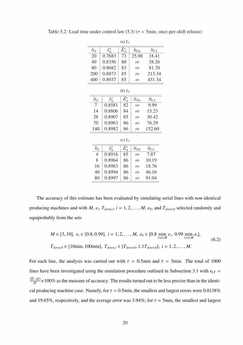
Table 5.2: Lead time under control law (5.3) (τ = 5min, once-per-shift release)

(a) L1

ltd e∗0 E∗S ltOL ltCL

20 0.7683 73 25.98 18.4140 0.8356 80 ∞ 38.2680 0.8682 83 ∞ 81.70

200 0.8873 85 ∞ 213.34400 0.8937 85 ∞ 431.34

(b) L2

ltd e∗0 E∗S ltOL ltCL

7 0.8581 82 ∞ 9.9914 0.8806 84 ∞ 15.2328 0.8907 85 ∞ 30.4270 0.8963 86 ∞ 76.29

140 0.8982 86 ∞ 152.60

(c) L3

ltd e∗0 E∗S ltOL ltCL

4 0.8916 85 ∞ 7.878 0.8964 86 ∞ 10.19

16 0.8983 86 ∞ 18.7640 0.8994 86 ∞ 46.1680 0.8997 86 ∞ 91.04

The accuracy of this estimate has been evaluated by simulating serial lines with non-identical

producing machines and with M, ei, Tdown,i, i = 1, 2, . . . , M, e0, and Tdown,0 selected randomly and

equiprobably from the sets

M ∈ [3, 10], ei ∈ [0.8, 0.99], i = 1, 2, . . . , M, e0 ∈ [0.8 min16i6M

ei, 0.99 min16i6M

ei],

Tdown,0 ∈ [10min, 100min], Tdown,i ∈ [Tdown,0, 1.1Tdown,0], i = 1, 2, . . . , M.(6.2)

For each line, the analysis was carried out with τ = 0.5min and τ = 5min. The total of 1000

lines have been investigated using the simulation procedure outlined in Subsection 3.1 with εLT =

|LT−LT |LT ×100% as the measure of accuracy. The results turned out to be less precise than in the identi-

cal producing machine case. Namely, for τ = 0.5min, the smallest and largest errors were 0.0138%

and 19.65%, respectively, and the average error was 3.94%; for τ = 5min, the smallest and largest

20

errors were 0.0037% and 19.00%, respectively, and the average error was 3.71%. However, when

ei’s were selected from sets ei ∈ [0.9, 0.99], i = 1, 2, . . . , M, and e0 ∈ [0.9 min16i6M

ei, 0.99 min16i6M

ei], the

accuracy was similar to that of the identical producing machine case: for τ = 0.5min, the smallest

and largest errors were 0.0002% and 9.71%, respectively, and the average error was 1.42%; for

τ = 5min, the smallest and largest errors were 0.0002% and 9.54%, respectively, and the average

error was 1.32%.

To further investigate LT defined by (6.1), introduce a modified relative load factor

ρmax :=e0

emin, (6.3)

where emin = min16i6M

ei, while keeping the relative lead time, lt, as in (3.3). Although reducing (6.1)

to an expression for lt(ρmax) seems to be formidable, the following upper bounds can be derived:

Proposition 6.2 Under the assumptions of Proposition 6.1,

lt 6 lt := 1 +1τ

(ρmax

Mµ0+

2M − 1Mµmin

emax

emin

)(1 − emin

1 − ρmax

), (6.4)

where emin = min16i6M

ei, emax = max16i6M

ei, and µmin = min16i6M

µi. Also, in the limit as M → ∞,

lt∞ := limM→∞

lt = 1 +

(2

τµmin

emax

emin

)(1 − emin

1 − ρmax

). (6.5)

These expressions again reduce to (3.4) and (3.5), respectively, if the producing machines are

identical. Also, all qualitative properties of (3.4) and (3.5) hold for (6.4) and (6.5) as well. For

instance, (6.5) does not depend on µ0, while (6.4) does. Finally, the rate of convergence of (6.4) to

(6.5) for µ0 > µmin, is also 12M (as in Section 3). So, the following chain of inequalities takes place:

lt(ρmax) 6 lt(ρmax) 6 lt∞(ρmax). (6.6)

This implies that if the release rate e0 is selected so that the bound (6.5) satisfies the desired lead

time, LTd, the system performance will be at least as good as LTd.

21

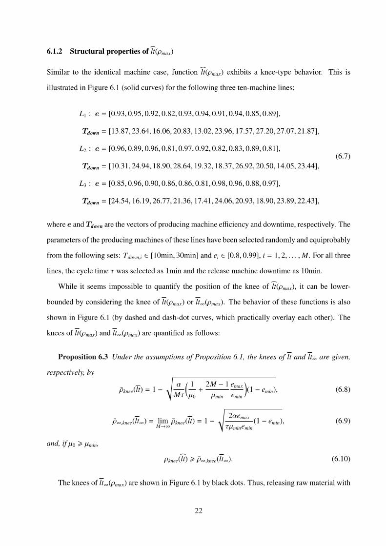
6.1.2 Structural properties of lt(ρmax)

Similar to the identical machine case, function lt(ρmax) exhibits a knee-type behavior. This is

illustrated in Figure 6.1 (solid curves) for the following three ten-machine lines:

L1 : e = [0.93, 0.95, 0.92, 0.82, 0.93, 0.94, 0.91, 0.94, 0.85, 0.89],

Tdown = [13.87, 23.64, 16.06, 20.83, 13.02, 23.96, 17.57, 27.20, 27.07, 21.87],

L2 : e = [0.96, 0.89, 0.96, 0.81, 0.97, 0.92, 0.82, 0.83, 0.89, 0.81],

Tdown = [10.31, 24.94, 18.90, 28.64, 19.32, 18.37, 26.92, 20.50, 14.05, 23.44],

L3 : e = [0.85, 0.96, 0.90, 0.86, 0.86, 0.81, 0.98, 0.96, 0.88, 0.97],

Tdown = [24.54, 16.19, 26.77, 21.36, 17.41, 24.06, 20.93, 18.90, 23.89, 22.43],

(6.7)

where e and Tdown are the vectors of producing machine efficiency and downtime, respectively. The

parameters of the producing machines of these lines have been selected randomly and equiprobably

from the following sets: Tdown,i ∈ [10min, 30min] and ei ∈ [0.8, 0.99], i = 1, 2, . . . , M. For all three

lines, the cycle time τ was selected as 1min and the release machine downtime as 10min.

While it seems impossible to quantify the position of the knee of lt(ρmax), it can be lower-

bounded by considering the knee of lt(ρmax) or lt∞(ρmax). The behavior of these functions is also

shown in Figure 6.1 (by dashed and dash-dot curves, which practically overlay each other). The

knees of lt(ρmax) and lt∞(ρmax) are quantified as follows:

Proposition 6.3 Under the assumptions of Proposition 6.1, the knees of lt and lt∞ are given,

respectively, by

ρknee(lt) = 1 −√

α

Mτ

( 1µ0

+2M − 1µmin

emax

emin

)(1 − emin), (6.8)

ρ∞,knee(lt∞) = limM→∞

ρknee(lt) = 1 −√

2αemax

τµminemin(1 − emin), (6.9)

and, if µ0 > µmin,

ρknee(lt) > ρ∞,knee(lt∞). (6.10)

The knees of lt∞(ρmax) are shown in Figure 6.1 by black dots. Thus, releasing raw material with

22

the load factor ρmax 6 ρ∞,knee ensures a safe system operation from the point of view of lead time.

0.7 0.8 0.9 10

400

800

1200

ρmax

lt

lt

lt

lt∞

(ρknee, ltknee)

(a) L1

0.7 0.8 0.9 10

400

800

1200

ρmax

lt

lt

lt

lt∞

(ρknee, ltknee)

(b) L2

0.7 0.8 0.9 10

400

800

1200

ρmax

lt

lt

lt

lt∞

(ρknee, ltknee)

(c) L3

Figure 6.1: Relative lead time, lt, as a function of relative workload, ρmax (for M = 10, τ = 1min)

6.2 Open-loop control

Proposition 6.4 Under the assumptions of Proposition 6.1, the sets of feasible lead times, Flt,

Flt, and Flt∞ , are given, respectively, by

lt > 1 +1

Mτ

( M∑

i=1

1 − ei

µi+

M−1∑

i=1

ei(1 − ei+1)µiei+1

),

lt > 1 + (1 − emin)2M − 1Mτµmin

emax

emin,

lt∞ > 1 +2(1 − emin)τµmin

emax

emin,

(6.11)

where emin = min16i6M

ei, emax = max16i6M

ei, and µmin = min16i6M

µi.

Proposition 6.5 Under the assumptions of Proposition 6.1, the release rate, e∗0, which ensures

the desired lead time, ltd ∈ Flt, is the unique real root less than min16i6M

ei of the following M-th order

polynomial equation:

(LTd−Mτ)M−1∏

i=0

(ei+1−e0)−(1−e1)( e0

µ0+

e1

µ1

) M−1∏

i=1

(ei+1−e0)−M−1∑

i=1

((1−ei+1)

( ei

µi+

ei+1

µi+1

) M−1∏

j=0, j,i

(e j+1−e0))

= 0.

(6.12)

For this release rate,

TP∗

=e∗0τ, WIP

∗0 =

e∗0τ

( e∗0µ0

+e1

µ1

)( 1 − e1

e1 − e∗0

), WIP

∗i =

e∗0τ

( ei

µi+

ei+1

µi+1

)( 1 − ei+1

ei+1 − e∗0

), i = 1, 2, . . . , M − 1.

(6.13)

23

Solving equation (6.12) might be too complex for practical applications. Therefore, using the

upper bounds lt and lt∞, we provide below more convenient lower bounds on e∗0.

Proposition 6.6 Let e∗0 and e∗0,∞ be the release rates that solve the open-loop lead time control

problem for lt and lt∞ with ltd ∈ {Flt ∩Flt ∩Flt∞}. Then,

e∗0 = emin

[1 −

µmin + (2M − 1)µ0emaxemin

Mµminµ0τ(ltd − 1) + µmin(1 − emin)(1 − emin)

], (6.14)

e∗0,∞ = emin

[1 −

2(1 − emin) emaxemin

τµmin(ltd − 1)

], (6.15)

and, if µ0 > µmin,

e∗0 > e∗0 > e∗0,∞. (6.16)

Similar to the identical machine case, the solution of the open-loop lead time control problem

for non-identical machines can be implemented by releasing raw material once-per-cycle with

probability e∗0 given by (6.14) with µ0 = ∞, i.e.,

p = emin

[1 −

(2M − 1) emaxemin

Mµminτ(ltd − 1)(1 − emin)

], (6.17)

or, for long lines, with p = e∗0,∞ given by (6.15).

The behavior of e∗0, e∗0, and e∗0,∞ is illustrated in Figure 6.2 (where black dots indicate the knee)

as a function of ltd for the three lines given in (6.7). From this figure, we conclude that, similar to

the identical machine case, raw material release with rates beyond the knee is not only unnecessary,

but detrimental as well.

6.3 Closed-loop control

The control law (5.3) remains applicable to the case of non-identical machines as well, with the

only difference that e∗0 in (4.14) and (5.2) is calculated according to either (6.12) or (6.14) or (6.15).

The closed-loop performance under this law remains roughly the same as for the identical machine

case; a detailed quantification of this performance is omitted due to space limitations.

24

0 500 1000 1500 20000.4

0.5

0.6

0.7

0.8

0.9

ltd

e∗ 0

e∗0

e∗0

e∗0,∞

(a) L1

0 500 1000 1500 20000.4

0.5

0.6

0.7

0.8

0.9

ltd

e∗ 0

e∗0

e∗0

e∗0,∞

(b) L2

0 500 1000 1500 20000.4

0.5

0.6

0.7

0.8

0.9

ltd

e∗ 0

e∗0

e∗0

e∗0,∞

(c) L3

Figure 6.2: Release rates, e∗0, e∗0, and e∗0,∞, as a function of the desired relative lead time, ltd (forM = 10)

7 Extensions

7.1 Asynchronous exponential lines

Although analytical methods for performance evaluation of asynchronous exponential lines are

readily available (see, for instance, [43]), and the lead time in these lines can be analyzed in full

details, due to space limitations, we discuss here only upper bounds on this performance measure.

Consider an asynchronous exponential line defined by assumptions (i)-(v). Assume that

τ0 = min16i6M

τi, TPisol,0 < min16i6M

TPisol,i, (7.1)

and, introduce the relative load factor as follows:

ρasync :=TPisol,0

min16i6M

TPisol,i. (7.2)

Along with this asynchronous line, consider an auxiliary synchronous line with the same re-

lease machine and the producing machines defined as follows:

τi = τ0, µi = µi, TPisol,i = TPisol,i, i = 1, 2, . . . , M. (7.3)

From these expressions, we obtain:

ei =τ0

τiei, λi =

µi

ei(1 − ei), i = 0, 1, . . . , M. (7.4)

25

With these parameters, the relative load factor for the auxiliary line, ρsync, is the same as for the

asynchronous one, i.e., given by (7.2). For the sake of brevity, we omit the subscript of both load

factors and denote them as ρ.

Let LTasync and LTsync denote the lead times of the original asynchronous line and the auxiliary

synchronous one, respectively. We analyze the relationship between LTasync and LTsync by simula-

tions. To accomplish this, we form 1000 asynchronous lines with parameters selected randomly

and equiprobably from the following sets:

M ∈ [3, 10], τi ∈ [0.8min, 1.2min], ei ∈ [0.7, 0.99], i = 1, 2, . . . , M,

TPisol,0 ∈ [0.7 min16i6M

TPisol,i, 0.99 min16i6M

TPisol,i],

Tdown,i ∈ [10min, 100min], i = 0, 1, . . . , M.

(7.5)

For each of these asynchronous lines, we form an auxiliary synchronous one according to (7.3)

and simulate the resulting 1000 pairs of lines using the procedure described in Subsection 3.1. As

a result, we obtain:

Observation 7.1 For all 1000 pairs of lines analyzed, LTasync < LTsync. The tightness of this

upper bound is 0.03 6 ∆LT 6 1.7, where ∆LT := LTsync−LTasync

LTasync.

7.2 Non-exponential lines

Since analytical methods for performance evaluation of non-exponential lines are not available,

the only tool for LT investigation is simulation. Using simulations, this subsection provides upper

bounds of LT for both synchronous and asynchronous cases.

26

7.2.1 Synchronous non-exponential lines

Consider non-exponential lines with ten identical machines having τ = 1min, Tdwon = 5min, and

other parameters selected as combinations from the following sets:

e ∈ {0.7, 0.8, 0.9}, ρ ∈ {0.7, 0.8, 0.9, 0.99},

Reliability model ∈ {Weibull, gamma, log-normal},

CV ∈ {0.01, 0.1, 0.25, 0.5, 0.75, 1},

(7.6)

where CV is the coefficient of variation of the machine reliability model. We confine the analysis

to CV 6 1 since, as it is shown in an empirical study [45], most of manufacturing equipment in

the automotive industry has CV’s of up- and downtimes less than 1, and an analytical study [46]

proves that if the breakdown and repair rates are increasing in time, the respective CV’s are again

less than 1.

Simulating the 216 lines, thus formed, we evaluate their lt shown in Table 7.1 by solid curves.

As one can see, lt is a monotonically increasing function of CV and, more importantly, it is practi-

cally independent of the machine reliability model.

Similar results have been obtained for synchronous lines with non-identical non-exponential

machines. An example is shown in Figure 7.1 for the three ten-machine lines with ei and Tdown,i

given in (6.7), τ = 1min, Tdown,0 = min16i6M

Tdown,i, ρmax = 0.9, and with the reliability models and

CV’s given in (7.6).

The curves of Table 7.1 and Figure 7.1 offer a possibility to introduce an upper bound on lt for

systems under consideration. Indeed, since lt for CV = 1 equals that of exponential lines, and the

smallest lt in any line is 1, the above mentioned simulation results lead to the following:

Observation 7.2 For all synchronous non-exponential lines analyzed in this subsection, lt is

upper-bounded by the following empirical formula (see the broken lines in Table 7.1 and Figure

7.1):

lt 6

(ltexp − 1)CV + 1, for 0.35 < CV 6 1,

0.35(ltexp − 1) + 1, for 0 < CV 6 0.35,(7.7)

27

where ltexp is the lt for the corresponding exponential line calculated according to (3.4) for identi-

cal machines or (3.3) and (6.1) for non-identical ones.

Table 7.1: Lead time for synchronous non-exponential lines with identical producing machines(M = 10)

e ρ0.7 0.8 0.9 0.99

0.7

0.8

0.9

0 0.25 0.5 0.75 1 5

10

15

20

25

30

CV

lt

Weibullgammalog−normalupper bound

(a) L1

0 0.25 0.5 0.75 1 0

10

20

30

40

CV

lt

Weibullgammalog−normalupper bound

(b) L2

0 0.25 0.5 0.75 1 5

10

15

20

25

30

CV

lt

Weibullgammalog−normalupper bound

(c) L3

Figure 7.1: Lead time for synchronous non-exponential lines with non-identical producing ma-chines (M = 10)

7.2.2 Asynchronous non-exponential lines

As in Subsection 7.1, we analyze asynchronous non-exponential lines by forming an auxiliary

synchronous exponential line and showing, by simulations, that lt of the latter can be used as ltexp

in the upper bound (7.7) for the former.

28

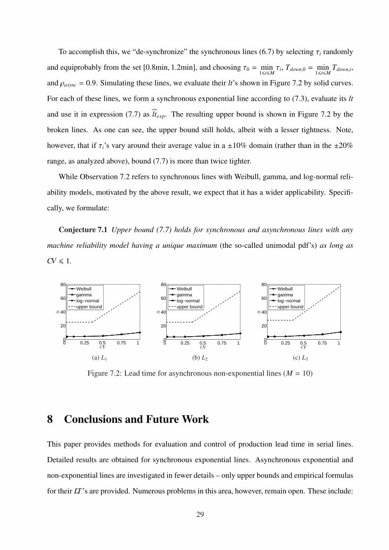
To accomplish this, we “de-synchronize” the synchronous lines (6.7) by selecting τi randomly

and equiprobably from the set [0.8min, 1.2min], and choosing τ0 = min16i6M

τi, Tdown,0 = min16i6M

Tdown,i,

and ρasync = 0.9. Simulating these lines, we evaluate their lt’s shown in Figure 7.2 by solid curves.

For each of these lines, we form a synchronous exponential line according to (7.3), evaluate its lt

and use it in expression (7.7) as ltexp. The resulting upper bound is shown in Figure 7.2 by the

broken lines. As one can see, the upper bound still holds, albeit with a lesser tightness. Note,

however, that if τi’s vary around their average value in a ±10% domain (rather than in the ±20%

range, as analyzed above), bound (7.7) is more than twice tighter.

While Observation 7.2 refers to synchronous lines with Weibull, gamma, and log-normal reli-

ability models, motivated by the above result, we expect that it has a wider applicability. Specifi-

cally, we formulate:

Conjecture 7.1 Upper bound (7.7) holds for synchronous and asynchronous lines with any

machine reliability model having a unique maximum (the so-called unimodal pdf’s) as long as

CV 6 1.

0 0.25 0.5 0.75 1 0

20

40

60

80

CV

lt

Weibullgammalog−normalupper bound

(a) L1

0 0.25 0.5 0.75 1 0

20

40

60

80

CV

lt

Weibullgammalog−normalupper bound

(b) L2

0 0.25 0.5 0.75 1 0

20

40

60

80

CV

lt

Weibullgammalog−normalupper bound

(c) L3

Figure 7.2: Lead time for asynchronous non-exponential lines (M = 10)

8 Conclusions and Future Work

This paper provides methods for evaluation and control of production lead time in serial lines.

Detailed results are obtained for synchronous exponential lines. Asynchronous exponential and

non-exponential lines are investigated in fewer details – only upper bounds and empirical formulas

for their LT ’s are provided. Numerous problems in this area, however, remain open. These include:

29

• Detailed analysis of LT in asynchronous exponential lines. This can be accomplished using,

for instance, the performance analysis technique developed in [43].

• Detailed investigation of LT in synchronous and asynchronous lines with non-exponential

machines. This can be accomplished by extensive simulations of systems at hand and in-

vestigating the tightness of the upper bounds on their LT ’s (based on auxiliary exponential

lines). This research may lead to validation or repudiation of Conjecture 7.1.

• Detailed analysis of feedback control laws for raw material release in asynchronous expo-

nential and non-exponential lines. The relay-type control law introduced in this paper could

be a starting point for this investigation. It seems likely that this control law may be applica-

ble to serial lines with arbitrary unimodal machine reliability model.

• Extension of the results obtained to re-entrant lines, where the lead time is known to be

exceptionally long, and the issue of limiting the lead time is of particular importance.

• Extension of the results obtained to assembly system, where the main line is fed by several

component lines, and the total lead time must be coordinated and controlled.

Solutions of these problems will result in a relatively complete and practical theory of lead time

in manufacturing systems and enable a novel paradigm for production management – maximize

the throughput under the constraint that the lead time takes the desired value.

Appendix

The analysis of LT for synchronous exponential lines is based on the recursive aggregation pro-

cedure described in [43]. For serial lines with M + 1 synchronous exponential machines defined

by (λ0, µ0), (λ1, µ1), . . . , (λM, µM) and M buffers with capacity N0,N1, . . . ,NM−1, the steady state of

this procedure, λ fi , µ f

i , i = 1, 2, . . . , M, and λbi , µb

i , i = 0, 1, . . . , M − 1, is the unique solution of the

30

following system of transcendental equations:

µfi = µi − µiQ(λ f

i−1, µfi−1, λ

bi , µ

bi ,Ni−1), 1 6 i 6 M,

λfi = λi + µiQ(λ f

i−1, µfi−1, λ

bi , µ

bi ,Ni−1), 1 6 i 6 M,

µbi = µi − µiQ(λb

i+1, µbi+1, λ

fi , µ

fi ,Ni), 0 6 i 6 M − 1,

λbi = λi + µiQ(λb

i+1, µbi+1, λ

fi , µ

fi ,Ni), 0 6 i 6 M − 1,

(A.1)

with the boundary conditions λ f0 = λ0, µ f

0 = µ0 and λbM = λM, µb

M = µM and

Q(x1, y1, x2, y2,N) =

(1−e1)(1−φ)1−φ exp(−βN) , if x1

y1, x2

y2,

x1(x1+x2)(y1+y2)(x1+y1)[(x1+x2)(y1+y2)+x2y1(x1+x2+y1+y2)N] , if x1

y1=

x2y2,

(A.2)

whereei =

yi

xi + yi, i = 1, 2,

φ =e1(1 − e2)e2(1 − e1)

,

β =(x1 + x2 + y1 + y2)(x1y2 − x2y1)

(x1 + x2)(y1 + y2).

(A.3)

The proofs of Propositions 3.1 and 6.1 are based on the following three lemmas, which extend

(A.1)-(A.3) to the case of Ni = ∞.

Lemma A.1 Function Q(x1, y1, x2, y2,N), defined by (A.2) and (A.3), has the following limit:

limN→∞

Q(x1, y1, x2, y2,N) =

0, if x1y16 x2

y2,

1 − e1e2, if x1

y1> x2

y2,

(A.4)

where ei =yi

xi+yi, i = 1, 2.

Proof: From (A.2),

• if x1y1

= x2y2

,

limN→∞

Q(x1, y1, x2, y2,N) = limN→∞

x1(x1 + x2)(y1 + y2)(x1 + y1)[(x1 + x2)(y1 + y2) + x2y1(x1 + x2 + y1 + y2)N]

= 0;(A.5)

31

• if x1y1< x2

y2, then

β =(x1 + x2 + y1 + y2)(x1y2 − x2y1)

(x1 + x2)(y1 + y2)< 0, (A.6)

and, thus,

limN→∞

Q(x1, y1, x2, y2,N) = limN→∞

(1 − e1)(1 − φ)1 − φ exp(−βN)

= 0; (A.7)

• if x1y1> x2

y2, then β > 0, and, therefore,

limN→∞

Q(x1, y1, x2, y2,N) = limN→∞

(1 − e1)(1 − φ)1 − φ exp(−βN)

= (1 − e1)(1 − φ)

= (1 − e1)(1 − e1(1 − e2)

e2(1 − e1)

)

= 1 − e1

e2.

(A.8)

�

Lemma A.2 Let e j = min{e1, e2, . . . , eM}, and j is the smallest index at which the minimum is

achieved. Let e fi := µ

fi

λfi +µ

fi

and ebi := µb

i

λbi +µb

i. Then, for Ni = ∞, i = 0, 1, . . . , M − 1,

e fi =

ei, if i < j,

e j, if i > j,eb

i =

e j, if i 6 j,

ei, if i > j,(A.9)

and the unique solution of (A.1) is

λfi = (λi + µi)(1 − e f

i ), µfi = (λi + µi)e

fi ,

λbi = (λi + µi)(1 − eb

i ), µbi = (λi + µi)eb

i .

(A.10)

Proof: We show that (A.9), (A.10) is the solution of (A.1) and then comment its uniqueness.

Since e j = min16i6M

ei, i.e., e j 6 ei, ∀i = 0, 1, . . . , M, we have

1 − e j

e j>

1 − ei

ei, ∀i = 0, 1, . . . , M. (A.11)

32

• If i < j, then based on (A.4), (A.9), (A.10), and (A.11), we have

Q(λ fi−1, µ

fi−1, λ

bi , µ

bi ,∞)

= Q[(λi−1 + µi−1)(1 − e f

i−1), (λi−1 + µi−1)e fi−1, (λi + µi)(1 − eb

i ), (λi + µi)ebi ,∞

]

= Q[(λi−1 + µi−1)(1 − ei−1), (λi−1 + µi−1)ei−1, (λi + µi)(1 − e j), (λi + µi)e j,∞]

= 0

(A.12)

and

Q(λbi+1, µ

bi+1, λ

fi , µ

fi ,∞)

= Q[(λi+1 + µi+1)(1 − eb

i+1), (λi+1 + µi+1)ebi+1, (λi + µi)(1 − e f

i ), (λi + µi)efi ,∞

]

= Q[(λi+1 + µi+1)(1 − e j), (λi+1 + µi+1)e j, (λi + µi)(1 − ei), (λi + µi)ei,∞]

= 1 − e j

ei.

(A.13)

Thus, for the left- and right-hand sides of the first equation of (A.1), we have, respectively,

µfi = (λi + µi)e

fi = (λi + µi)ei = µi (A.14)

and

µi − µiQ(λ fi−1, µ

fi−1, λ

bi , µ

bi ,∞) = µi, (A.15)

implying that (A.9) and (A.10) solve the first equation of (A.1) for i < j. Similarly, for the

left- and right-hand sides of the second equation of (A.1), we have,

λfi = (λi + µi)(1 − e f

i ) = (λi + µi)(1 − ei) = λi (A.16)

and

λi + µiQ(λ fi−1, µ

fi−1, λ

bi , µ

bi ,∞) = λi, (A.17)

implying that (A.9) and (A.10) solve the second equation of (A.1) for i < j. For the third

33

equation of (A.1), the left- and right-hand sides are respectively

µbi = (λi + µi)eb

i = (λi + µi)e j (A.18)

and

µi − µiQ(λbi+1, µ

bi+1, λ

fi , µ

fi ,∞) = µi

e j

ei= (λi + µi)e j, (A.19)

implying that (A.9) and (A.10) solve the third equation of (A.1) for i < j. As for the last

equation of (A.1), the left- and right-hand sides are

λbi = (λi + µi)(1 − eb

i ) = (λi + µi)(1 − e j) (A.20)

and

λi + µiQ(λbi+1, µ

bi+1, λ

fi , µ

fi ,∞) = λi + µi

(1 − e j

ei

)= (λi + µi)(1 − e j), (A.21)

implying that (A.9) and (A.10) solve the last equation of (A.1) for i < j.

• If i = j, the two Q-functions in (A.1) are respectively

Q(λ fi−1, µ

fi−1, λ

bi , µ

bi ,∞)

= Q[(λi−1 + µi−1)(1 − e f

i−1), (λi−1 + µi−1)e fi−1, (λi + µi)(1 − eb

i ), (λi + µi)ebi ,∞

]

= Q[(λi−1 + µi−1)(1 − ei−1), (λi−1 + µi−1)ei−1, (λi + µi)(1 − e j), (λi + µi)e j,∞]

= 0

(A.22)

and

Q(λbi+1, µ

bi+1, λ

fi , µ

fi ,∞)

= Q[(λi+1 + µi+1)(1 − eb

i+1), (λi+1 + µi+1)ebi+1, (λi + µi)(1 − e f

i ), (λi + µi)efi ,∞

]

= Q[(λi+1 + µi+1)(1 − ei+1), (λi+1 + µi+1)ei+1, (λi + µi)(1 − e j), (λi + µi)e j,∞]

= 0.

(A.23)

34

Thus, the left- and right-hand sides of (A.1) are

µfi = (λi + µi)e

fi = (λi + µi)e j = (λi + µi)ei = µi,

µi − µiQ(λ fi−1, µ

fi−1, λ

bi , µ

bi ,∞) = µi,

λfi = (λi + µi)(1 − e f

i ) = (λi + µi)(1 − e j) = (λi + µi)(1 − ei) = λi,

λi + µiQ(λ fi−1, µ

fi−1, λ

bi , µ

bi ,∞) = λi,

µbi = (λi + µi)eb

i = (λi + µi)e j = (λi + µi)ei = µi,

µi − µiQ(λbi+1, µ

bi+1, λ

fi , µ

fi ,∞) = µi,

λbi = (λi + µi)(1 − eb

i ) = (λi + µi)(1 − e j) = (λi + µi)(1 − ei) = λi,

λi + µiQ(λbi+1, µ

bi+1, λ

fi , µ

fi ,∞) = λi,

(A.24)

implying that (A.1) is solved for i = j.

• If i > j, the two Q-functions in (A.1) are

Q(λ fi−1, µ

fi−1, λ

bi , µ

bi ,∞)

= Q[(λi−1 + µi−1)(1 − e f

i−1), (λi−1 + µi−1)e fi−1, (λi + µi)(1 − eb

i ), (λi + µi)ebi ,∞

]

= Q[(λi−1 + µi−1)(1 − e j), (λi−1 + µi−1)e j, (λi + µi)(1 − ei), (λi + µi)ei,∞]

= 1 − e j

ei

(A.25)

and

Q(λbi+1, µ

bi+1, λ

fi , µ

fi ,∞)

= Q[(λi+1 + µi+1)(1 − eb

i+1), (λi+1 + µi+1)ebi+1, (λi + µi)(1 − e f

i ), (λi + µi)efi ,∞

]

= Q[(λi+1 + µi+1)(1 − ei+1), (λi+1 + µi+1)ei+1, (λi + µi)(1 − e j), (λi + µi)e j,∞]

= 0.

(A.26)

35

Thus, the left- and right-hand sides of (A.1) are

µfi = (λi + µi)e

fi = (λi + µi)e j,

µi − µiQ(λ fi−1, µ

fi−1, λ

bi , µ

bi ,∞) = µi

e j

ei= (λi + µi)e j,

λfi = (λi + µi)(1 − e f

i ) = (λi + µi)(1 − e j),

λi + µiQ(λ fi−1, µ

fi−1, λ

bi , µ

bi ,∞) = λi + µi

(1 − e j

ei

)= (λi + µi)(1 − e j),

µbi = (λi + µi)eb

i = (λi + µi)ei = µi,

µi − µiQ(λbi+1, µ

bi+1, λ

fi , µ

fi ,∞) = µi,

λbi = (λi + µi)(1 − eb

i ) = (λi + µi)(1 − ei) = λi,

λi + µiQ(λbi+1, µ

bi+1, λ

fi , µ

fi ,∞) = λi,

(A.27)

which also implies that (A.1) is solved.

As far as the uniqueness of (A.9) and (A.10) is concerned, it follows directly from Theorem

11.4 of [43]. �

Lemma A.3 In synchronous exponential two-machine lines with e1 < e2,

limN→∞

WIP =e1

τ

( e1

µ1+

e2

µ2

)( 1 − e2

e2 − e1

). (A.28)

Proof: From the proof of Theorem 11.3 in [43], we know that

limN→∞

WIP = limN→∞

D5

D2 + D3= lim

N→∞

D2−K

D2 + D3, (A.29)

where limN→∞

D2 = − 2+D1+ 1D1

K , D1 =µ1+µ2λ1+λ2

, K =(λ1+λ2+µ1+µ2)(λ2µ1−λ1µ2)

(λ1+λ2)(µ1+µ2) , D3 =(λ1+λ2+µ1+µ2)(λ2+µ1)+λ1µ2−λ2µ1

λ2µ1(λ1+λ2+µ1+µ2) .

Thus, we have

36

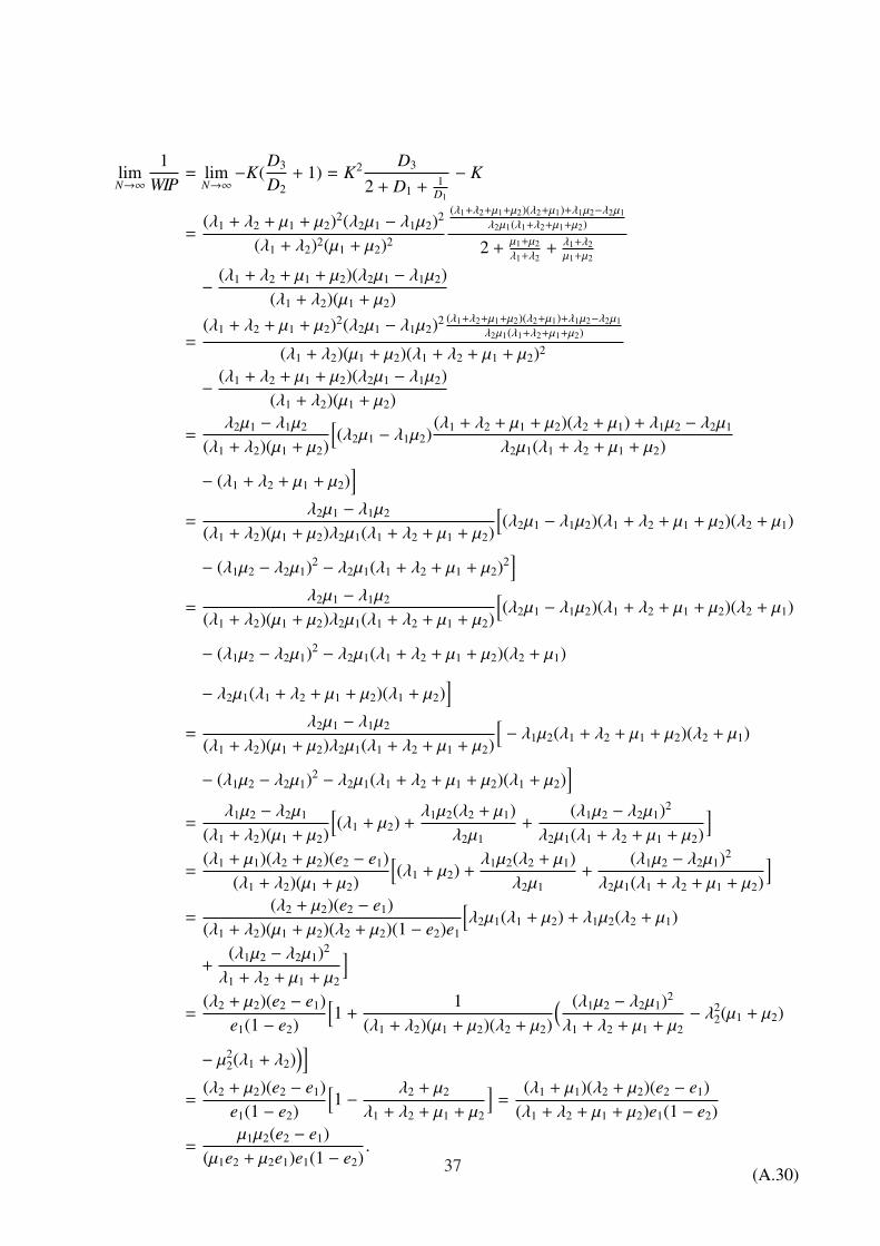
limN→∞

1WIP

= limN→∞−K(

D3

D2+ 1) = K2 D3

2 + D1 + 1D1

− K

=(λ1 + λ2 + µ1 + µ2)2(λ2µ1 − λ1µ2)2

(λ1 + λ2)2(µ1 + µ2)2

(λ1+λ2+µ1+µ2)(λ2+µ1)+λ1µ2−λ2µ1λ2µ1(λ1+λ2+µ1+µ2)

2 +µ1+µ2λ1+λ2

+ λ1+λ2µ1+µ2

− (λ1 + λ2 + µ1 + µ2)(λ2µ1 − λ1µ2)(λ1 + λ2)(µ1 + µ2)

=(λ1 + λ2 + µ1 + µ2)2(λ2µ1 − λ1µ2)2 (λ1+λ2+µ1+µ2)(λ2+µ1)+λ1µ2−λ2µ1

λ2µ1(λ1+λ2+µ1+µ2)

(λ1 + λ2)(µ1 + µ2)(λ1 + λ2 + µ1 + µ2)2

− (λ1 + λ2 + µ1 + µ2)(λ2µ1 − λ1µ2)(λ1 + λ2)(µ1 + µ2)

=λ2µ1 − λ1µ2

(λ1 + λ2)(µ1 + µ2)

[(λ2µ1 − λ1µ2)

(λ1 + λ2 + µ1 + µ2)(λ2 + µ1) + λ1µ2 − λ2µ1

λ2µ1(λ1 + λ2 + µ1 + µ2)

− (λ1 + λ2 + µ1 + µ2)]

=λ2µ1 − λ1µ2

(λ1 + λ2)(µ1 + µ2)λ2µ1(λ1 + λ2 + µ1 + µ2)

[(λ2µ1 − λ1µ2)(λ1 + λ2 + µ1 + µ2)(λ2 + µ1)

− (λ1µ2 − λ2µ1)2 − λ2µ1(λ1 + λ2 + µ1 + µ2)2]

=λ2µ1 − λ1µ2

(λ1 + λ2)(µ1 + µ2)λ2µ1(λ1 + λ2 + µ1 + µ2)

[(λ2µ1 − λ1µ2)(λ1 + λ2 + µ1 + µ2)(λ2 + µ1)

− (λ1µ2 − λ2µ1)2 − λ2µ1(λ1 + λ2 + µ1 + µ2)(λ2 + µ1)

− λ2µ1(λ1 + λ2 + µ1 + µ2)(λ1 + µ2)]

=λ2µ1 − λ1µ2

(λ1 + λ2)(µ1 + µ2)λ2µ1(λ1 + λ2 + µ1 + µ2)

[− λ1µ2(λ1 + λ2 + µ1 + µ2)(λ2 + µ1)

− (λ1µ2 − λ2µ1)2 − λ2µ1(λ1 + λ2 + µ1 + µ2)(λ1 + µ2)]

=λ1µ2 − λ2µ1

(λ1 + λ2)(µ1 + µ2)

[(λ1 + µ2) +

λ1µ2(λ2 + µ1)λ2µ1

+(λ1µ2 − λ2µ1)2

λ2µ1(λ1 + λ2 + µ1 + µ2)

]

=(λ1 + µ1)(λ2 + µ2)(e2 − e1)

(λ1 + λ2)(µ1 + µ2)

[(λ1 + µ2) +

λ1µ2(λ2 + µ1)λ2µ1

+(λ1µ2 − λ2µ1)2

λ2µ1(λ1 + λ2 + µ1 + µ2)

]

=(λ2 + µ2)(e2 − e1)

(λ1 + λ2)(µ1 + µ2)(λ2 + µ2)(1 − e2)e1

[λ2µ1(λ1 + µ2) + λ1µ2(λ2 + µ1)

+(λ1µ2 − λ2µ1)2

λ1 + λ2 + µ1 + µ2

]

=(λ2 + µ2)(e2 − e1)

e1(1 − e2)

[1 +

1(λ1 + λ2)(µ1 + µ2)(λ2 + µ2)

( (λ1µ2 − λ2µ1)2

λ1 + λ2 + µ1 + µ2− λ2

2(µ1 + µ2)

− µ22(λ1 + λ2)

)]

=(λ2 + µ2)(e2 − e1)

e1(1 − e2)

[1 − λ2 + µ2

λ1 + λ2 + µ1 + µ2

]=

(λ1 + µ1)(λ2 + µ2)(e2 − e1)(λ1 + λ2 + µ1 + µ2)e1(1 − e2)

=µ1µ2(e2 − e1)

(µ1e2 + µ2e1)e1(1 − e2).

(A.30)37

Therefore,

limN→∞

WIP =(µ1e2 + µ2e1)e1(1 − e2)

µ1µ2(e2 − e1)= e1

( e1

µ1+

e2

µ2

)( 1 − e2

e2 − e1

). (A.31)

In [43], (A.29) is derived for τ = 1. For general τ, (A.28) follows (see proofs for Chapter 11 in

Chapter 20 of [43]). �

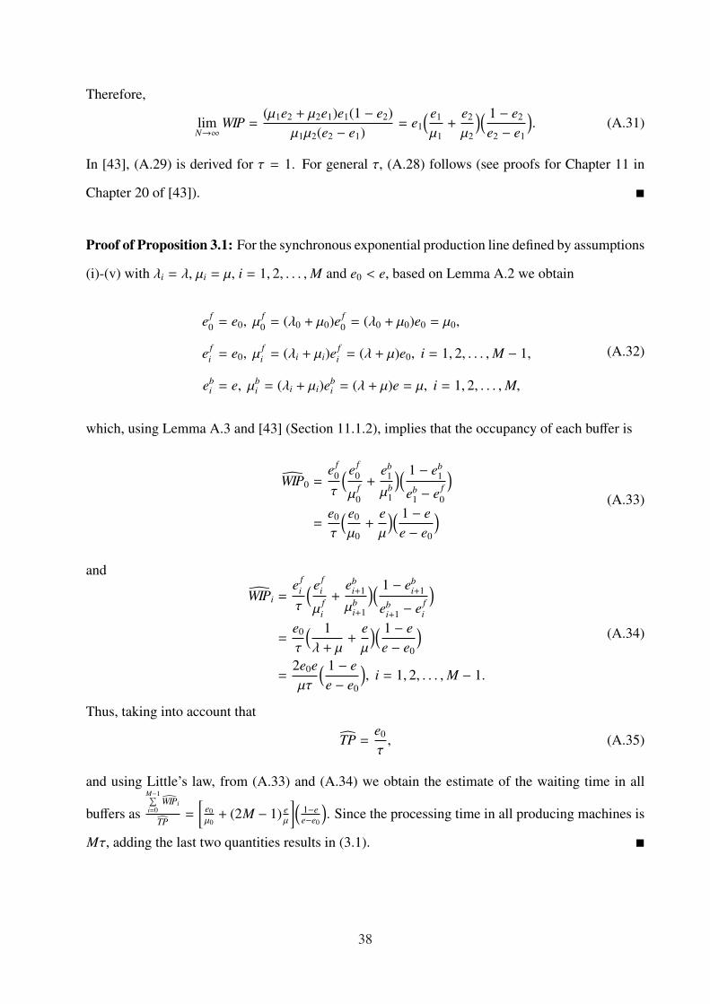
Proof of Proposition 3.1: For the synchronous exponential production line defined by assumptions

(i)-(v) with λi = λ, µi = µ, i = 1, 2, . . . , M and e0 < e, based on Lemma A.2 we obtain

e f0 = e0, µ

f0 = (λ0 + µ0)e f

0 = (λ0 + µ0)e0 = µ0,

e fi = e0, µ

fi = (λi + µi)e

fi = (λ + µ)e0, i = 1, 2, . . . , M − 1,

ebi = e, µb

i = (λi + µi)ebi = (λ + µ)e = µ, i = 1, 2, . . . , M,

(A.32)

which, using Lemma A.3 and [43] (Section 11.1.2), implies that the occupancy of each buffer is

WIP0 =e f

0

τ

( e f0

µf0

+eb

1

µb1

)( 1 − eb1

eb1 − e f

0

)

=e0

τ

( e0

µ0+

eµ

)( 1 − ee − e0

) (A.33)

and

WIPi =e f

i

τ

( e fi

µfi

+eb

i+1

µbi+1

)( 1 − ebi+1

ebi+1 − e f

i

)

=e0

τ

( 1λ + µ

+eµ

)( 1 − ee − e0

)

=2e0eµτ

( 1 − ee − e0

), i = 1, 2, . . . , M − 1.

(A.34)

Thus, taking into account that

TP =e0

τ, (A.35)

and using Little’s law, from (A.33) and (A.34) we obtain the estimate of the waiting time in all

buffers as

M−1∑i=0

WIPi

TP=

[e0µ0

+ (2M − 1) eµ

](1−ee−e0

). Since the processing time in all producing machines is

Mτ, adding the last two quantities results in (3.1). �

38

Proof of Proposition 3.2: Let

f (ρ) := αlt(ρ) = α(1 +

1Mτ

( ρµ0

+2M − 1

µ

)(1 − e1 − ρ

)). (A.36)

Thenf ′(ρ) =

α

Mτ

( 1µ0

+2M − 1

µ

) 1 − e(1 − ρ)2 ,

f ′′(ρ) =2αMτ

( 1µ0

+2M − 1

µ

) 1 − e(1 − ρ)3 ,

and, therefore,

κ(f (ρ)

)=

∣∣∣ f ′′ρρ∣∣∣

(1 + f ′2ρ )32

=

2αMτ

( 1µ0

+ 2M−1µ

)(1 − e)

[(1 − ρ)2 + α2

M2τ2

( 1µ0

+ 2M−1µ

)2 (1−e)2

(1−ρ)2

] 32

. (A.37)

Since ρknee = arg maxρ κ(f (ρ)

), differentiating (A.37) and solving for ρ, we obtain (3.9). Clearly,

when M tends to infinity, (3.9) becomes (3.10). �

Proof of Proposition 4.1: As it follows from (3.4), lt is an increasing function of ρ. Since 0 < ρ <

1, this implies that

lt > 1 + (1 − e)2M − 1

MTdown

τ. (A.38)

For M → ∞ the above inequality becomes

lt∞ > 1 + 2(1 − e)Tdown

τ. (A.39)

�

Proof of Proposition 4.2: From (3.4) it follows that

ρ∗ = 1 − µ + (2M − 1)µ0

Mµµ0τ(ltd − 1) + µ(1 − e)(1 − e), (A.40)

which implies that (4.2) holds. As for (4.3), it follows immediately from the proof of Proposition

3.1. �

39

Proof of Proposition 6.1: Similar to the proof of Proposition 3.1, with the only difference that,

instead of (A.32), we have

e fi = e0, µ

fi = (λi + µi)e

fi = (λi + µi)e0, i = 0, 1, . . . , M − 1,

ebi = ei, µ

bi = (λi + µi)eb

i = (λi + µi)ei = µi, i = 1, 2, . . . , M,(A.41)

and, therefore,

WIP0 =e f

0

τ

( e f0

µf0

+eb

1

µb1

)( 1 − eb1

eb1 − e f

0

)

=e0

τ

( e0

µ0+

e1

µ1

)( 1 − e1

e1 − e0

),

(A.42)

WIPi =e f

i

τ

( e fi

µfi

+eb

i+1

µbi+1

)( 1 − ebi+1

ebi+1 − e f

i

)

=e0

τ

( 1λi + µi

+ei+1

µi+1

)( 1 − ei+1

ei+1 − e0

)

=e0

τ

( ei

µi+

ei+1

µi+1

)( 1 − ei+1

ei+1 − e0

), i = 1, 2, . . . , M − 1.

(A.43)

�

Proof of Proposition 6.2: From (6.1) and (3.3), we obtain

lt = 1 +1

Mτ

M−1∑

i=0

( ei

µi+

ei+1

µi+1

)( 1 − ei+1

ei+1 − e0

). (A.44)

Thus,

lt 6 1 +1

Mτ

M−1∑

i=0

( ei

µi+

ei+1

µi+1

)( 1 − emin

emin − e0

)

6 1 +1

Mτ

( e0

µ0+ (2M − 1)

emax

µmin

)( 1 − emin

emin − e0

)

= 1 +1τ

(ρmax

Mµ0+

2M − 1Mµmin

emax

emin

)( 1 − emin

1 − ρmax

).

(A.45)

�

40

Proof of Proposition 6.3: Similar to the proof of Proposition 3.2, with the only difference that

f (ρmax) : = αlt(ρmax) = α

(1 +

1Mτ

(ρmax

µ0+

2M − 1µmin

emax

emin

)( 1 − emin

1 − ρmax

)),

f ′(ρmax) =α

Mτ

( 1µ0

+2M − 1µmin

emax

emin

) 1 − emin

(1 − ρmax)2 ,

f ′′(ρmax) =2αMτ

( 1µ0

+2M − 1µmin

emax

emin

) 1 − emin

(1 − ρmax)3 ,

and, therefore, we obtain (6.8). When M tends to infinity, (6.8) becomes (6.9).

In the following, we focus on proving (6.10), Let

f (ρmax) := α{1 +

1Mτ

M−1∑

i=0

( ei

µi+

ei+1

µi+1

)( 1 − ei+1

ei+1 − e0

)}. (A.46)

Since ρknee(lt) is the ρmax that maximize the curvature of f (ρmax), to prove (6.10), we need to prove

that

κ(f (ρmax)

)=

| f ′′(ρmax)|(1 + f ′2(ρmax)

) 32

(A.47)

is an increasing function of ρmax ∈ (0, ρ∞,knee], where ρ∞,knee is defined in (6.9). In other words, we

need to prove

κ′(f (ρmax)

)=

f ′′′(ρmax)(1 + f ′2(ρmax)

) − 3 f ′(ρmax) f ′′2(ρmax)(1 + f ′2(ρmax)

) 52

> 0 (A.48)

for all ρmax ∈ (0, ρ∞,knee], where

f ′(ρmax) =α

Mτemin

[( e1

µ0+

e1

µ1

) 1 − e1( e1emin− ρmax

)2 +

M−1∑

i=1

( ei

µi+

ei+1

µi+1

) 1 − ei+1( ei+1emin− ρmax

)2

],

f ′′(ρmax) =2α

Mτemin

[( e1

µ0+

e1

µ1

) 1 − e1( e1emin− ρmax

)3 +

M−1∑

i=1

( ei

µi+

ei+1

µi+1

) 1 − ei+1( ei+1emin− ρmax

)3

],

f ′′′(ρmax) =6α

Mτemin

[( e1

µ0+

e1

µ1

) 1 − e1( e1emin− ρmax

)4 +

M−1∑

i=1

( ei

µi+

ei+1

µi+1

) 1 − ei+1( ei+1emin− ρmax

)4

].

(A.49)

41

Let

γ1 =( e1

µ0+

e1

µ1

)(1 − e1), γi+1 =

( ei

µi+

ei+1

µi+1

)(1 − ei+1), i = 1, 2, . . . , M − 1,

ηi =1

eiemin− ρmax

, i = 1, 2, . . . , M.(A.50)

Then, proving (A.48) implies proving

12

( M∑

i=1

γiη4i

)[(Mτemin

α

)2+

( M∑

i=1

γiη2i

)2]>

( M∑

i=1

γiη2i

)( M∑

i=1

γiη3i

)2

. (A.51)

Based on (6.9) and considering that µ0 > µmin, we obtain

Mτemin

α=

2Memax(1 − emin)µmin(1 − ρ∞,knee)2 >

M∑

i=1

γi

(1 − ρ∞,knee)2 >M∑

i=1

γiη2i , ∀ρmax ∈ (0, ρ∞,knee]. (A.52)

Thus, (A.51) becomes ( M∑

i=1

γiη4i

)( M∑

i=1

γiη2i

)>

( M∑

i=1

γiη3i

)2

, (A.53)

i.e., Cauchy-Schwarz inequality, which completes the proof. �

Proof of Proposition 6.4: Rewriting (6.1) as

LT − Mτ =e0

µ0

( 1 − e1

e1 − e0

)+

e1

µ1

( 1 − e1

e1 − e0

)+

M−1∑

i=1

( ei

µi+

ei+1

µi+1

)( 1 − ei+1

ei+1 − e0

)

=1 − e1

µ0

( e1

e1 − e0− 1

)+

e1

µ1

( 1 − e1

e1 − e0

)+

M−1∑

i=1

( ei

µi+

ei+1

µi+1

)( 1 − ei+1

ei+1 − e0

),

(A.54)

and taking into account that 0 < e0 < min16i6M

ei, we observe that the right-hand side of (A.54) is a

monotonically increasing function of e0. Thus,

LT − Mτ >

M∑

i=1

1 − ei

µi+

M−1∑

i=1

ei(1 − ei+1)µiei+1

, (A.55)

i.e., the first inequality in (6.11) holds. The second and the third inequalities are derived similarly

using (6.4) and (6.5), respectively. �

42

Proof of Proposition 6.5: Under the assumptions of Proposition 6.1, for any desired lead time LTd

satisfying (6.11), the release rate e∗0 that ensures this lead time is a real root less than min16i6M

ei of the

equation

LTd = Mτ +

M−1∑

i=0

( ei

µi+

ei+1

µi+1

)( 1 − ei+1

ei+1 − e0

). (A.56)

Rewrite the above equation as follows:

LTd − Mτ =1 − e1

µ0

( e1

e1 − e0− 1

)

+e1

µ1

( 1 − e1

e1 − e0

)+

M−1∑

i=1

( ei

µi+

ei+1

µi+1

)( 1 − ei+1

ei+1 − e0

).

(A.57)

Since the right-hand side of (A.57) is a monotonically increasing function of e0 when 0 < e0 <

min16i6M

ei, equation (A.57) (or (A.56)) has a unique real solution less than min16i6M

ei ensuring the desired

lead time LTd. Multiplying (A.56) byM−1∏j=0

(e j+1 − e0) and re-arranging the terms, we obtain (6.12).

In other words, for any desired lead time LTd satisfying (6.11), the release rate e∗0 that ensures this

lead time is the unique real root less than min16i6M

ei of the M-th order polynomial equation (6.12).

The statements on TP∗

and WIP∗

follow from the proof of Proposition 6.1. �

Proof of Proposition 6.6: Solving the equation in (6.4) with lt = ltd, we obtain

ρ∗max = 1 −µmin + (2M − 1)µ0

emaxemin

Mµminµ0τ(ltd − 1) + µmin(1 − emin)(1 − emin). (A.58)

This, taking into account (6.3), results in (6.14). Expression (6.15) is obtained similarly using

(6.5).

Clearly, if µ0 > µmin, then (6.6) holds, which implies that (6.16) holds as well. �

References

[1] J. H. Blackstone Jr., D. T. Phillips, and G. L. Hogg, “A state-of-the-art survey of dispatching

rules for manufacturing job shop operations,” International Journal of Production Research,

43

vol. 20, no. 1, pp. 27–45, 1982.

[2] R. T. Barrett and S. N. Kadipasaoglu, “Dispatching rules for a dynamic flow shop,” Produc-

tion and Inventory Management Journal, vol. 31, no. 1, pp. 54–58, 1990.

[3] A. M. Waikar, B. R. Sarker, and A. M. Lal, “A comparative study of some priority dispatching

rules under different shop loads,” Production Planning & Control, vol. 6, no. 4, pp. 301–310,

1995.

[4] Y.-F. Hung and I.-R. Chen, “A simulation study of dispatch rules for reducing flow times in

semiconductor wafer fabrication,” Production Planning & Control, vol. 9, no. 7, pp. 714–722,

1998.

[5] C. Rajendran and O. Holthaus, “A comparative study of dispatching rules in dynamic flow-

shops and jobshops,” European Journal of Operational Research, vol. 116, no. 1, pp. 156–

170, 1999.

[6] M. L. Pinedo, Scheduling: Theory, Algorithms, and Systems, 4th ed. Springer, 2012.

[7] A. Hubl, H. Jodlbauer, and K. Altendorfer, “Influence of dispatching rules on average pro-

duction lead time for multi-stage production systems,” International Journal of Production

Economics, vol. 144, no. 2, pp. 479–484, 2013.

[8] Y. Sugimori, K. Kusunoki, F. Cho, and S. Uchikawa, “Toyota production system and kanban

system materialization of just-in-time and respect-for-human system,” International Journal

of Production Research, vol. 15, no. 6, pp. 553–564, 1977.

[9] G. R. Bitran and L. Chang, “A mathematical programming approach to a deterministic kanban

system,” Management Science, vol. 33, no. 4, pp. 427–441, 1987.

[10] L. J. Krajewski, B. E. King, L. P. Ritzman, and D. S. Wong, “Kanban, MRP, and shaping the

manufacturing environment,” Management Science, vol. 33, no. 1, pp. 39–57, 1987.

[11] D. Mitra and I. Mitrani, “Analysis of a kanban discipline for cell coordination in production

lines. I,” Management Science, vol. 36, no. 12, pp. 1548–1566, 1990.

44

[12] B. J. Berkley, “A review of the kanban production control research literature,” Production

and Operations Management, vol. 1, no. 4, pp. 393–411, 1992.

[13] S. R. Tayur, “Structural properties and a heuristic for kanban-controlled serial lines,” Man-

agement Science, vol. 39, no. 11, pp. 1347–1368, 1993.

[14] J. A. Muckstadt and R. T. Sridhar, “A comparison of alternative kanban control mechanisms.

I: Background and structural results,” IIE Transactions, vol. 27, no. 2, pp. 140–150, 1995.

[15] M. Di Mascolo, Y. Frein, and Y. Dallery, “An analytical method for performance evaluation

of kanban controlled production systems,” Operations Research, vol. 44, no. 1, pp. 50–64,

1996.

[16] M. S. Akturk and F. Erhun, “An overview of design and operational issues of kanban sys-

tems,” International Journal of Production Research, vol. 37, no. 17, pp. 3859–3881, 1999.

[17] M. Lage Jr. and M. G. Filho, “Variations of the kanban system: Literature review and classi-

fication,” International Journal of Production Economics, vol. 125, no. 1, pp. 13–21, 2010.

[18] E. Topan and Z. M. Avsar, “An approximation for kanban controlled assembly systems,”

Annals of Operations Research, vol. 182, no. 1, pp. 133–162, 2011.

[19] J. Matzka, M. Di Mascolo, and K. Furmans, “Buffer sizing of a heijunka kanban system,”

Journal of Intelligent Manufacturing, vol. 23, no. 1, pp. 49–60, 2012.

[20] R. Sato and Y. Khojasteh-Ghamari, “An integrated framework for card-based production con-

trol systems,” Journal of Intelligent Manufacturing, vol. 23, no. 3, pp. 717–731, 2012.

[21] M. L. Spearman, D. L. Woodruff, and W. J. Hopp, “CONWIP: A pull alternative to kanban,”

International Journal of Production Research, vol. 28, no. 5, pp. 879–894, 1990.

[22] I. Duenyas and W. J. Hopp, “Estimating the throughput of an exponential CONWIP assembly

system,” Queueing Systems, vol. 14, no. 1, pp. 135–157, 1993.

45

[23] W. J. Hopp and M. L. Roof, “Setting WIP levels with statistical throughput control (STC) in

CONWIP production lines,” International Journal of Production Research, vol. 36, no. 4, pp.

867–882, 1998.

[24] A. M. Bonvik, Y. Dallery, and S. B. Gershwin, “Approximate analysis of production sys-

tems operated by a CONWIP/finite buffer hybrid control policy,” International Journal of

Production Research, vol. 38, no. 13, pp. 2845–2869, 2000.

[25] W. G. Gilland, “A simulation study comparing performance of CONWIP and bottleneck-

based release rules,” Production Planning & Control, vol. 13, no. 2, pp. 211–219, 2002.

[26] J. M. Framinan, P. L. Gonzalez, and R. Ruiz-Usano, “The CONWIP production control sys-

tem: Review and research issues,” Production Planning & Control, vol. 14, no. 3, pp. 255–

265, 2003.

[27] J. Geraghty and C. Heavey, “A comparison of hybrid push/pull and CONWIP/pull production

inventory control policies,” International Journal of Production Economics, vol. 91, no. 1, pp.

75–90, 2004.

[28] S. Gstettner and H. Kuhn, “Analysis of production control systems kanban and CONWIP,”

International Journal of Production Research, vol. 34, no. 11, pp. 3253–3273, 1996.

[29] K. K. Yang, “Managing a flow line with single-kanban, dual-kanban or CONWIP,” Produc-

tion and Operations Management, vol. 9, no. 4, pp. 349–366, 2000.

[30] H. Jodlbauer and A. Huber, “Service-level performance of MRP, kanban, CONWIP and DBR

due to parameter stability and environmental robustness,” International Journal of Production

Research, vol. 46, no. 8, pp. 2179–2195, 2008.

[31] Y. Khojasteh-Ghamari, “A performance comparison between kanban and CONWIP con-

trolled assembly systems,” Journal of Intelligent Manufacturing, vol. 20, no. 6, pp. 751–760,

2009.

46

[32] ——, “Developing a framework for performance analysis of a production process controlled

by kanban and CONWIP,” Journal of Intelligent Manufacturing, vol. 23, no. 1, pp. 61–71,

2012.

[33] L. Zhang, “Kanban-controlled exponential produciton lines: Analysis and design,” Journal

of Manufacturing Technology Management, vol. 24, no. 3, pp. 358–383, 2013.

[34] A. Azaron, H. Katagiri, K. Kato, and M. Sakawa, “Modelling complex assemblies as a queue-

ing network for lead time control,” European Journal of Operational Research, vol. 174,

no. 1, pp. 150–168, 2006.

[35] A. Azaron and F. Kianfar, “A multi-objective lead time control problem in multistage assem-

bly systems using an interactive method,” Applied Mathematics and Computation, vol. 176,

no. 2, pp. 609–620, 2006.

[36] C. Perkgoz, A. Azaron, H. Katagiri, K. Kato, and M. Sakawa, “A multi-objective lead time

control problem in multi-stage assembly systems using genetic algorithms,” European Jour-

nal of Operational Research, vol. 180, no. 1, pp. 292–308, 2007.

[37] S. Yaghoubi, S. Noori, and F. Pourdadashi-Komachali, “Lead time control in multi-server

multi-stage assembly system,” The International Journal of Advanced Manufacturing Tech-

nology, vol. 61, no. 1-4, pp. 351–368, 2012.

[38] S. Yaghoubi, S. Noori, and A. Azaron, “Lead time control in multi-class multi-stage assembly

systems with finite capacity,” Computers & Industrial Engineering, vol. 66, no. 4, pp. 808–

817, 2013.

[39] C.-J. Kuo, C.-F. Chien, and J.-D. Chen, “Manufacturing intelligence to exploit the value of

production and tool data to reduce cycle time,” IEEE Transactions on Automation Science

and Engineering, vol. 8, no. 1, pp. 103–111, 2011.

[40] G. Chen, L. Zhang, J. Arinez, and G. Xiao, “Analysis of production completion time in

Bernoulli serial lines with finite buffers,” in IEEE International Conference on Automation

Science and Engineering, 2013, pp. 770–775.

47

[41] S. Biller, S. M. Meerkov, and C.-B. Yan, “Raw material release rates to ensure desired pro-

duction lead time in Bernoulli serial lines,” International Journal of Production Research,

vol. 51, no. 14, pp. 4349–4364, 2013.

[42] S. M. Meerkov and C.-B. Yan, “Cellular production lines with asymptotically reliable

Bernoulli machines: Lead time analysis and control,” 2014, accepted for publication in IEEE

Transactions on Automation Science and Engineering.

[43] J. Li and S. M. Meerkov, Production Systems Engineering. New York: Springer, 2009.

[44] R. Courant and F. John, Introduction to Calculus and Analysis. Springer, 1999, vol. 1.

[45] R. R. Inman, “Empirical evaluation of exponential and independence assumptions in queue-

ing models of manufacturing systems,” Production and Operations Management, vol. 8,

no. 4, pp. 409–432, 1999.

[46] J. Li and S. M. Meerkov, “On the coefficients of variation of uptime and downtime in man-

ufacturing equipment,” Mathematical Problems in Engineering, vol. 2005, no. 1, pp. 1–6,

2005.

48