Embed Size (px)
Citation preview

Environment for Development
Discussion Paper Series June 2008 EfD DP 08-20
Production Function Analysis of Soil Properties and Soil Conservation Investments in Tropical Agriculture
Anders Ekbom and Thomas S te rner

Environment for Development
The Environment for Development (EfD) initiative is an environmental economics program focused on international research collaboration, policy advice, and academic training. It supports centers in Central America, China, Ethiopia, Kenya, South Africa, and Tanzania, in partnership with the Environmental Economics Unit at the University of Gothenburg in Sweden and Resources for the Future in Washington, DC. Financial support for the program is provided by the Swedish International Development Cooperation Agency (Sida). Read more about the program at www.efdinitiative.org or contact [email protected].
Central America Environment for Development Program for Central America Centro Agronómico Tropical de Investigacíon y Ensenanza (CATIE) Email: [email protected]
China Environmental Economics Program in China (EEPC) Peking University Email: [email protected]
Ethiopia Environmental Economics Policy Forum for Ethiopia (EEPFE) Ethiopian Development Research Institute (EDRI/AAU) Email: [email protected]
Kenya Environment for Development Kenya Kenya Institute for Public Policy Research and Analysis (KIPPRA) Nairobi University Email: [email protected]
South Africa Environmental Policy Research Unit (EPRU) University of Cape Town Email: [email protected]
Tanzania Environment for Development Tanzania University of Dar es Salaam Email: [email protected]

© 2008 Environment for Development. All rights reserved. No portion of this paper may be reproduced without permission of the authors.
Discussion papers are research materials circulated by their authors for purposes of information and discussion. They have not necessarily undergone formal peer review.
Production Function Analysis of Soil Properties and Soil Conservation Investments in Tropical Agriculture
Anders Ekbom and Thomas Sterner
Abstract This paper integrates traditional economic variables, soil properties, and variables on soil
conservation technologies in order to estimate agricultural output among small-scale farmers in Kenya’s central highlands. The study has methodological and empirical, as well as policy, implications.
The key methodological finding is that integrating traditional economics and soil science is valuable in this area of research. Omitting measures of soil capital can cause omitted-variables bias because a farmer’s choice of inputs depends both on the quality and status of the soil plus other economic conditions, such as availability and cost of labor, fertilizers, manure, and other inputs.
The study shows that models which include soil capital and soil conservation technologies yield a considerably lower output elasticity of farmyard manure, and that mean output elasticities of key soil nutrients, such as nitrogen and potassium, are positive and relatively large. Counter to expectations, the mean output elasticity of phosphorus is negative. Soil conservation technologies (green manure and terraces, for example) are positively associated with output and yield relatively large output elasticities.
The central policy implication is that while fertilizers are generally beneficial, their application is a complex art, and more is not necessarily better. The limited local market supply of fertilizers, combined with the different output effects of nitrogen, potassium, and phosphorus highlight the importance of improving the performance of input markets and strengthening agricultural extension. Further, given the policy debate on the impact (and usefulness) of government subsidies on soil conservation, the results suggest that soil conservation investments contribute to an increase in farmers’ output. Consequently, government support for appropriate soil conservation investments arrests soil erosion, prevents downstream externalities, such as siltation of dams, rivers, and coastal zones, and helps farmers increase food production and food security.
Key Words: micro-analysis of farm firms, resource management
JEL Classification: Q12, Q20

Contents
Introduction............................................................................................................................. 1
1. Crop Production in Kenya ................................................................................................ 2
2. The Study Area ................................................................................................................... 3
3. Choice of Model................................................................................................................... 7
4. Data Collection and Definition of Variables.................................................................... 9
5. Statistical Results .............................................................................................................. 12
5.1 Agricultural Labor ..................................................................................................... 14
5.2 Chemical Fertilizer and Manure ................................................................................ 15
5.3 Agricultural Land....................................................................................................... 15
5.4 Green Manure ............................................................................................................ 15
5.5 Soil Conservation Terraces ........................................................................................ 16
5.6 Access to Public Infrastructure .................................................................................. 16
5.7 Soil Capital................................................................................................................. 17
5.8 Sensitivity Analysis ................................................................................................... 20
6. Summary and Conclusions.............................................................................................. 22
References.............................................................................................................................. 25
Appendices............................................................................................................................. 32
Appendix 1 Correlation Coefficients of Soil Properties ............................................... 32
Appendix 2 Correlation Coefficients of Soil Conservation Quality Variables............. 33
Appendix 3 Definition of Variables.............................................................................. 34
Appendix 4 Regression Results of Models UM, RM1, and RM2 ................................ 35
Appendix 5a Estimates of Translog Restrictions on UM, RM1, and RM2 .................. 37
Appendix 5b Pearson Correlation Coefficients of Output Elasticities ......................... 37
Appendix 6 Regression Results of Models UM’, RM1’, and RM2.............................. 38
Appendix 7 Estimates of Translog Restrictions on UM’, RM1’, and RM2 ................. 39
Environment for Development Ekbom and Sterner
1
Product Function Analysis in Soil Properties and Soil Conservation Investments in Tropical Agriculture
Anders Ekbom and Thomas Sterner∗
Introduction
The purpose of this paper is to increase our understanding of the determinants of agricultural production by integrating models and methods from economics and soil science. We took the opportunity to synthesize two areas of analysis: economic studies typically do not include soil variables, and soil studies typically focus exclusively on soil properties and other biophysical variables. The vast majority of economic studies that fit agricultural production functions to empirical data focuses on variables, such as labor, capital, and technology; and inputs, such as chemical fertilizers, farmyard manure, and pesticides (see, e.g., Deolalikar and Vijverberg 1987; Widawsky et al. 1998; Carrasco-Tauber and Moffitt 1992; Fulginiti and Perrin 1998; Gerdin 2002). Certainly, there are exceptions to these generalizations. Sherlund et al. (2002), for instance, also included a set of environmental variables; Nkonya et al. (2004) used data from Uganda to identify determinants of soil nutrient balances in small-scale crop production; Mundlak et al. (1997) estimated the role of potential dry matter and water availability for crop production in a cross-country analysis.
Agronomic or soil-scientific studies have contributed to our understanding of the biophysical factors in agricultural production (see, e.g., Rutunga et al. 1998; Hartemink et al. 2000; Mureithi et al. 2003). However, these types of studies generally do not explain the role of economic factors. The analyses are usually done in repeated field trials on controlled plots at research stations and exclude capital, labor, and other vital production factors. Consequently, key issues, such as labor productivity, are rarely estimated (Smaling et al. 1993; Hartemink et al. 2000). More importantly, omitting labor and agricultural capital will bias all other results, and
∗ Anders Ekbom, Environmental Economics Unit, Department of Economics, University of Gothenburg, Box 640, SE 405 30 Gothenburg, Sweden, (tel) + 46-31-786 4817, (fax) + 46-31-786 4154, (email) [email protected]; and Thomas Sterner, Department of Economics, University of Gothenburg, P.O. Box 640, 405 30 Gothenburg, Sweden, (email) [email protected], (fax) +46 31 7861326. Thanks to Gardner Brown, E. Somanathan, Ed Barbier, Johan Rockström, Arne Bigsten, Gunnar Köhlin, Peter Berck, Lennart Flood, Daniela Andrén, Martin Linde-Rahr, Menale Kassie, and Adrian Müller, whose advice and helpful comments on this paper are much appreciated. Financial support from Sida (Swedish International Development and Cooperation Agency) is also gratefully acknowledged.
Environment for Development Ekbom and Sterner
2
ultimately the problem is that controlled field experiments have little similarity to real agriculture. As an example, omitting labor in controlled experiments of the “optimal application” of fertilizer neglects the trade-off or substitution between labor (to ameliorate the soil) and fertilizer. The implicit price of agricultural labor partly determines the supply of fertilizer. This applies to several inputs for which labor functions as a substitute or a complement.
1. Crop Production in Kenya
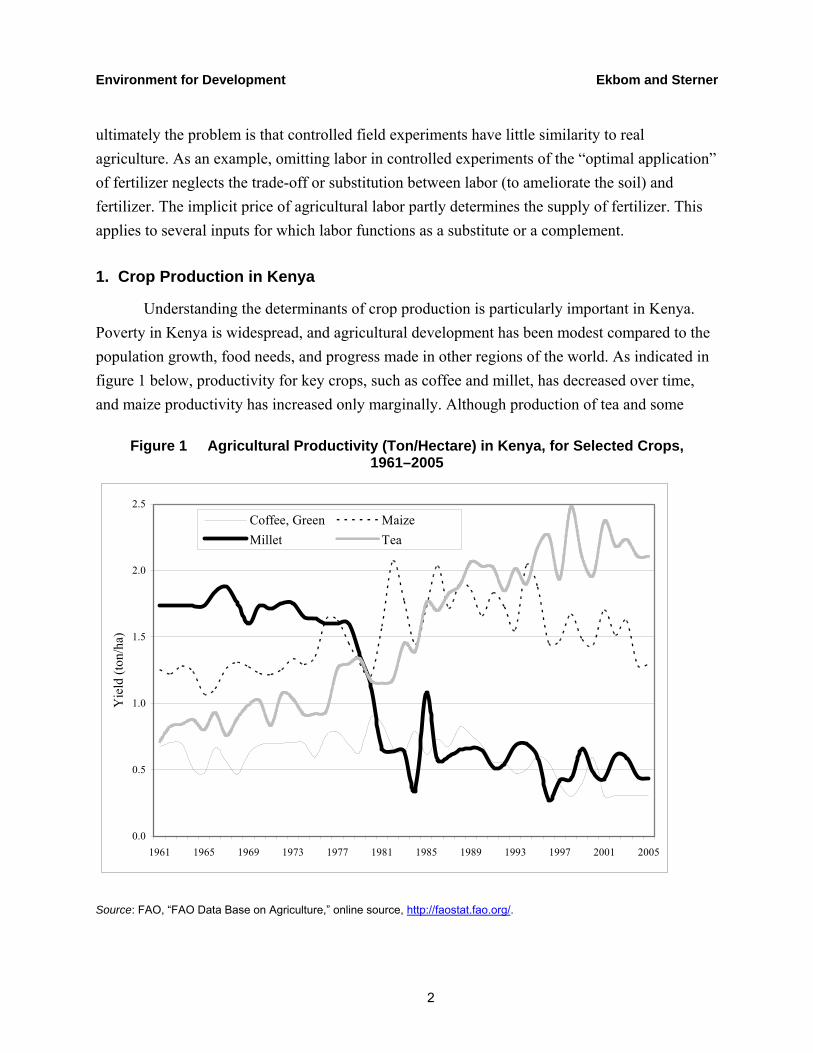
Understanding the determinants of crop production is particularly important in Kenya. Poverty in Kenya is widespread, and agricultural development has been modest compared to the population growth, food needs, and progress made in other regions of the world. As indicated in figure 1 below, productivity for key crops, such as coffee and millet, has decreased over time, and maize productivity has increased only marginally. Although production of tea and some
Figure 1 Agricultural Productivity (Ton/Hectare) in Kenya, for Selected Crops, 1961–2005
0.0
0.5
1.0
1.5
2.0
2.5
1961 1965 1969 1973 1977 1981 1985 1989 1993 1997 2001 2005
Yie
ld (t
on/h
a)
Coffee, Green MaizeMillet Tea
Source: FAO, “FAO Data Base on Agriculture,” online source, http://faostat.fao.org/.
Environment for Development Ekbom and Sterner
3
other crops has increased over time, the average population growth of 3.2 percent (1961–2005) and poor performance in the agricultural sector have actually reduced food production per capita over this period.
Many economic studies have attempted to explain Kenya’s agricultural performance (see, e.g., Gerdin 2002), but they typically have little or no information on soil capital and soil change, despite the fact that soil is a key asset in agricultural production, and that soil erosion significantly depreciates soil capital, reduces crop yields, and significantly increases costs to society. As one indication, costs of soil erosion in Kenya may translate into losses of 3.8 percent of GDP. This cost equals Kenya’s total annual electricity production or agricultural exports (Cohen et al. 2006). Hidden costs of this magnitude and the lack of integration between traditional economic factors, soil conservation investments, and soil properties prompted this particular study.
The paper is organized into 6 sections. Section 2 presents the field study area. The production function model and the key equations to be estimated empirically are in section 3. Section 4 presents the data, while section 5 discusses the statistical results, and section 6 summarizes the results and draws some policy conclusions.
2. The Study Area
The study area is located in Muranga District, which is part of the fertile agricultural areas in Kenya’s highlands. It is located at around 1500 meters above sea level, south of Mount Kenya and southeast of the Aberdares forest reserve, which form a large watershed of the Indian Ocean. It has two rainy seasons with mean annual precipitation of 1560 mm (Ovuka and Lindqvist 2000) and shares many demographic, socio-economic, and biophysical features with other districts in the central highlands. Given the area’s importance for Kenya’s total employment and food production, understanding agricultural production in this area has broad policy relevance.
In the summary statistics in table 1, mean agricultural output of each household amounts to around KSh 38,000 (US$ 543),1 subject to some variation. Generally, farmers living in the
1 US$ 1 = KSh 70.

Environment for Development Ekbom and Sterner
4
area are poor by international standards: a majority live on less than $2 per capita per day, and 30–40 percent of the population are below the poverty line (< $1 per capita per day). Consequently, the level of technology is very low (usually only a hoe and panga2 for tilling) and the amount of agricultural inputs is also very low.
Table 1 Summary of Descriptive Statistics
Variable Variable definition Mean Min. Max. Std. dev.
Q Output (KSh) 38313 2050 304450 43252
LQ Agric. Labor supply: (hours/year) 1407 90 6060 980
F Chemical fertilizer (KSh) 3504 0 14400 2543.8
P Pesticides (KSh) 211 0 18000 1235
M Manure (KSh) 6343 0 40000 7428
K Agricultural land area (acres) 2.4 0.2 8.0 1.3
I1 Green manure (rating 0–10) 0.8 0 8 1.9
I2 Terrace quality (rating 0–10) 5.8 0 10 2
I3 Distance coffee factory (miles) 2011 100 12000 1835
I4 Tree capital (number of coffee trees) 144 0 526 97
H1 Sex of household head (1=M; 0=F) 0.7 0 1 0.5
H2 Age of household head (years) 55.1 20 96 13.9
H3 Education of household head (years) 5.7 0 20 4.4
H4 Livestock capital (KSh) 23778 0 150250 20729
H5 Age of coffee trees (years) 22.4 0 54 11.6
H6 Family size (number of members) 4.2 1 13 2.2
Labor constitutes the major input (> 1400 hours per year). Although there is some variation, the average farm spends only around KSh 10,000 (US$ 143) per year on chemical fertilizers, pesticides, and manure. As an indicator of land scarcity and fragmentation, the mean
2 Similar to a machete with a broader blade.

Environment for Development Ekbom and Sterner
5
land area used for agricultural production by each household is only 2.4 acres,3 cultivated by four family members on average. Due to subdivision, the farms in the area are distributed in narrow strips sloping downwards from sharp ridges. A typical farm stretches from the ridge crest some 100–150 meters down the slope to the valley bottom until it reaches a stream or a river. The slopes are steep with mean farm gradients ranging between 20–60 percent. The homestead is typically located at the crest, and garden fruits and vegetables are cultivated around it.
The largest share of the agricultural land is allocated to food crops, such as maize, beans, potatoes, kale (sukuma wiki), and bananas. Minor food crops include yams, sorghum, and cassava. Tree crops grown and sold include papayas, avocados, macadamia nuts, and mangoes. A sizeable share of the farm area is allocated for cash-crop production, which implies mono-cultivation of coffee (Arabica) on bench terraces. Around the homestead, fruits and vegetables (e.g., lemons, limes, oranges, mangoes, tomatoes, cabbage, lettuce) are cultivated.
Although most of the agricultural activities are carried out by women, 70 percent of the households are headed by older men (mean age 55 years). The remaining 30 percent consists of widows, divorced women, or female-headed households where the men more or less permanently work elsewhere. The level of formal education is low. Slightly more than half of the adults can read and write and have an average of less than six years of schooling. Although poverty is widespread, most households possess some livestock capital. As indicated in table 1, the variation among households is considerable. Nevertheless, mean livestock holding amounts to KSh 24,000 (US$ 343), which is usually a cow, one or two goats, and some poultry. The distance to public infrastructure is far. For instance, the nearest coffee factory is on average more than 2 km away, via characteristic hilly and slippery rural foot trails. Coffee (like most crops) is carried to the factories (or the local market) as head loads in sacks. Even though the major source of income is on-farm agriculture, many of the households also obtain income from on-farm non-agricultural work or off-farm work.4
3 The mean farm size is 2.8 acres. Some land is allocated to the homestead, grazing, and woodlots, or classified as wasteland. 4 On-farm non-agricultural work usually includes brewing, brick-making, baking, pottery, shoe-making, wood carving, repairs, sewing, or similar and practical low-skill types of work. Off-farm incomes are derived from work as a guard, driver, small shop owner, street vendor, and casual laborer on someone else’s farm. Semi-skilled work is found in small-scale grain mills, coffee factories, or milk- and fruit-processing plants. In a few cases, skilled work as school teacher, nurse, etc., is available.

Environment for Development Ekbom and Sterner
6
Table 2 below shows some summary statistics of the soil properties. The main soil type cultivated in the area is a reddish clay (humic nitisol), from weathered basic volcanic rock. It is generally categorized as fertile, but is prone to heavy leaching and erosion, which reduce fertility considerably (Sombroek et al. 1982).
Table 2 Summary Statistics of Soil Properties
Soil property Unit Mean Min. Max. Std. dev.
pH-level (H2O solution) -log H+ 5.63 4.1 8.2 0.66
Carbon (C) % 1.51 0.16 2.81 0.45
Organic matter % 2.59 0.28 4.83 0.78
Nitrogen (N) % 0.18 0.08 0.6 0.06
Potassium (K) m.eq./100 g. 2.36 0.15 11 1.73
Sodium (Na) m.eq./100 g. 0.14 0 0.6 0.19
Calcium (Ca) m.eq./100 g. 6.48 1.45 20 3.29
Magnesium (Mg) m.eq./100 g. 5.26 0.02 17.42 2.81
Cation exchange capacity m.eq./100 g. 15.69 0 36.8 5.49
Phosphorus (P) ppm 17.84 1 195 24.67
Sand texture % 16.4 5 50 6.85
Clay texture % 63.16 28 82 10.59
Based on geographical comparisons and laboratory analysis (Thomas 1997), the soil samples statistics indicate that the soils in the study area are generally acidic, have moderate amounts of carbon and organic matter, and have low cation exchange capacity. Despite information of this kind, it is difficult to say something a priori about the soil’s productivity or fertility. The difficulty arises partly because crops respond very differently to different proportions and absolute amounts of soil properties, partly because each crop is endogenously chosen and adapted to each plot. Besides the impacts of external factors—rainfall, temperature, sunlight, etc.—the difficulty is compounded by the different responses of the soils and crops to various combinations of inputs, such as mineral fertilizers and farmyard manure (Thomas 1997; Gachene and Kimaru 2003). Consequently, individual outcomes are unique and “soil productivity” is essentially an empirical issue.
For our purposes, we wanted to identify agricultural output, given the actual distribution of soil properties and farming system (crop mix, choice of inputs, etc.) observed on each farm.

Environment for Development Ekbom and Sterner
7
3. Choice of Model
In our model, we assumed the farmers produced output (Q) by a specific choice of traditional economic production factors (Z), other variables (I), and soil capital (S). As indicated in equation (1) below, we assumed a modified translog function:5
1ln( ) ln( ) ln( ) ln( ) ln( )2i i ij i j k k l l
i i j k lQ Z Z Z I S uα β β γ δ= + + + + +∑ ∑ ∑ ∑ ∑ , (1)
where the first part is a traditional translog with conventional economic variables (labor, capital, etc.), expanded in the second part with investments (I) and soil capital (S). α , iβ , ijβ , kγ , and lδ
are the parameter coefficients to be estimated. u denotes the error term, which is assumed to be normally distributed and represents unexplained factors such as rainfall, sunlight, and temperature.
Z is a vector of traditional agricultural physical inputs, including labor (L), fertilizers (F), manure (M), and agricultural land (K). Arguably, these inputs are independent of the error term, since most of the decisions on the type, amount, and use of inputs are made prior to the time output is realized. The physical inputs of these production factors are chosen in different proportions by the farmer and are thus variable in the short run. Hence, Z is a choice variable.
I is a vector of variables pertaining to soil conservation investments, access to public infrastructure, and tree capital. S represents original, underlying properties of the soil. Although we lacked data on these particular properties, we did have data on certain soil properties (Sl; l=1..n), which may serve as proxies for S. However, as shown in Ekbom (2007), these soil properties are functions of other variables:
ˆlS = f(H, I, X, PF, R), (2)
where H represents a vector of household characteristics, I is a vector of variables representing soil conservation investments, X represents technical extension advice provided to farmers on soil and water conservation, and PF is a vector of physical production factors used in the
5 Indeed, many functional forms are conceivable, but since the true technology is unknown and cannot be determined a priori, the choice of appropriate functional form is essentially an empirical issue (Guilkey et al. 1983). Our choice was motivated by the fact that the translog is flexible (Christensen et al. 1973; Simmons and Weiserbs 1979) and has been used in many empirical investigations of agricultural production (see, e.g., Sherlund et al. 2002; Jacoby 1992, 1993; Skoufias 1994; and Gerdin 2002).

Environment for Development Ekbom and Sterner
8
agriculture. R is a vector representing variables on crop allocation. Equations 1 and 2, therefore, represent a recursive system, which implies that we should use ˆ
lS as substitutes for lS . Hence,
the empirical estimations will be based on the following equation:
1ˆ ˆln( ) ln( ) ln( ) ln( ) ln( )2i i ij i j k k l l
i i j k lQ Z Z Z I S uα β β γ δ= + + + + +∑ ∑ ∑ ∑ ∑ . (3)
Qualitatively, the rationale behind estimating equation 3 instead of equation 1 is due to the possibility that some variables have an impact on output directly, while others have both a direct effect and an indirect effect via their effect on soil (S).
The factors represented by I and S may be altered in the long run, but are fixed in the short run. This assumption stipulates separability between Z, I, and S in the estimations. The definition of each variable is given a more thorough explanation in section 3.
In order to estimate equation 3, we regressed equations (2) and (3) in two steps. First, we produced predicted values of Sl by SUR (seemingly unrelated regression) analysis of equation 2; second, we estimated equation 3 by OLS (ordinary least squares regression) after including the predicted values of soil capital ˆ( )lS as instrumental variables (IV) for Sl. Regularity conditions of
the translog production imply that linear homogeneity and symmetry will be satisfied if:
1, 0i iji i
β β= =∑ ∑ and ij jiβ β=
for i, j = 1, …, n and monotonicity is satisfied if the estimated factor shares are positive.6 In the econometric specification, we imposed linear homogeneity and symmetry.7
As point of departure, we used a comprehensive set of variables believed to explain agricultural output (see section 4 below), in order to estimate a universal model (UM) of equation 3. We used likelihood ratio tests (LRTs) as a formal method of model choice by nesting
6 Concavity is satisfied if the Hessian matrix of second-order derivatives is negative semi-definite (i.e., its eigenvalues are non-positive). This regularity condition, however, cannot be fulfilled here; production on some farms yields negative output elasticities. The usual assumption of cost minimization in production cannot be attained in our context, arguably due to imperfect information on, e.g., soil status at the farm level. Soil capital and soil conservation technologies are also fixed in the short term and therefore cannot be used in optimal proportions.
7 The specific restrictions imposed on the model are the following: β1+β2+β3+β4 = 1; β11 + 0.5*β12 + 0.5*β13 +
0.5*β34 = 0; 0.5*β12 + β22 + 0.5*β23 + 0.5*β24 = 0; 0.5*β13 + 0.5*β23 + β33 + 0.5*β34 = 0; 0.5*β14 + 0.5*β24 + 0.5*β34
+ β44 = 0. For estimation statistics of the translog model restrictions, see appendices 5 and 7, respectively.
Environment for Development Ekbom and Sterner
9
two restricted models and testing down from the universal model. The first restricted model (RM1) includes a sub-set of the variables included in UM (including the predicted values of soil capital and soil conservation investments). The other restricted model (RM2) includes only “traditional” economic variables,8 namely agricultural labor, fertilizers, manure, and land.
Even in a seemingly homogeneous setting, individual conditions may vary considerably. We therefore estimated individual output elasticities for each household.
As a sensitivity test of model robustness, we also performed a regression analysis of equation 1, where lS is represented by actual field measures of soil capital, i.e., chemical and
physical soil properties, such as pH, carbon, nitrogen, phosphorus, potassium, and grain size-distribution.
4. Data Collection and Definition of Variables
The data used in our analysis was obtained from a household survey collected in 1998. Based on a random sample, 252 small-scale farm households were identified for the survey and interviews took place between June and August 1998. The interviewed farmers hold approximately 20 percent of the total number of farms in the study area.
Output (Q): The farmers in the area produce approximately 30 different crops on farms of various sizes, averaging six crops per farm. Output is aggregated using local market prices. The value of agricultural output produced by each household (Q) is derived by multiplying each household’s physical production of crop i (qi) by the local market price (pi), i iQ p q= ∑ . Coffee
is the main cash crop. Maize, beans, potatoes, kale, and bananas are the key food or subsistence crops. Output from agro-forestry or tree crops (mangoes, avocados, lemons, papayas, and macadamia nuts, etc.) are included in aggregated output.
Labor, fertilizer, and manure:9 Agricultural labor (LQ) includes all labor for agricultural production activities, such as preparing the seed bed, sowing, weeding, thinning, and harvesting. It is measured by the number of hours worked during the last year of cultivation,
8
21ln( ) ln( ) ln( ) ln( )2RM i i ij i j
i i jQ Z Z Zα β β ε= + + +∑ ∑ ∑
9 Although some farmers (approximately 15%) also use pesticides in their production, pesticides were not included in the model, since there are strong reasons to believe that pests are part of the error term. Pests are commonly treated reactively (i.e., mitigated when a pest has broken out and has been observed ) and may be correlated with other inputs.

Environment for Development Ekbom and Sterner
10
covering two growing seasons. It includes adult family labor and hired labor. It excludes labor allocated to soil conservation investments (e.g., digging cut-off drains or maintaining terraces) because soil conservation is a long-term effort with inter-temporal impacts picked up by S and I.
Farmers use inorganic fertilizers, which are available on the market in different brands, chemical compositions, and physical units. Farmers also use farmyard manure from poultry or livestock in their cultivation. Due to heterogeneity in physical units and types, production factors (fertilizers and manure) and output are aggregated by their local market price (ci), respectively:
i iF c F= ∑ and i iM c M= ∑ .
Soil capital: Data on soil capital (Sl) were obtained from physical soil samples collected during the same period from all farms. The soil samples were taken at 0–15 cm depth from the topsoil, based on three replicates in each farm field (shamba). Places where mulch, manure, and chemical fertilizer were visible were avoided for soil sampling. The soil samples were air dried and analyzed at the University of Nairobi’s Department of Soil Science (DSS).10 Analysis of correlation coefficients showed correlation between some soil properties (see appendix 1). In order to avoid multicollinearity, the restricted model (RM1) includes only uncorrelated soil properties.
Soil conservation investments (I): The data on soil conservation investments were defined in terms of a quality rating. The rating was derived from a practical expert-assessment framework for evaluating soil conservation technologies (described in Thomas 1995; and Thomas et al. 1997). The soil conservation technologies were measured on a rating scale of 0–10 according to standard criteria for quality assessment by field technical assistants. Generally, a higher rating implies a higher quality of specific conservation investments to arrest soil erosion, prevent land degradation, and maintain soil moisture and fertility. The specific soil conservation technologies used in the econometric analysis (green manure, terraces) constitute a subset of a larger data set of soil conservation variables (appendix 2). These are common soil conservation technologies in the area and represent both biological conservation measures (green manure) and physical measures (terraces).
10 Total nitrogen (N) was analyzed by the Kjeldahl method. Potassium (K) was determined using flame photometer. Available phosphorus (P) was analyzed using the Mehlich method. Further details of the standard analytical methods used at the DSS can be found in Okalebo et al. (1993), Ekbom and Ovuka (2001), and Ovuka (2000).

Environment for Development Ekbom and Sterner
11
Green manure (I1): A form of conservation tillage, this biological conservation technology enhances agricultural productivity. Practicing green manure is a soil capital investment which, in general terms, builds up the soil’s physical, chemical, structural, and biological properties. Specifically, it implies planting cover crops, (e.g., legumes or grasses), for the combined purpose of reducing the soil’s erodibility, increasing organic matter content, building up the soil’s physical structure, maintaining soil moisture, and improving the soil’s fertility. It is interesting to study because it has the potential to boost yields and conserve soil (Mureithi et al. 2003). Green manure is practiced as part of an integrated nutrient management system (Woomer et al. 1999).
Soil conservation terraces (I2): In Kenya, these typically are excavated, backward-sloping bench terraces created by throwing soil uphill (fanya juu) or downhill (fanya chini) to form soil bunds (ridges) along the contour. As the soil erodes, they gradually develop into full terraces. Commonly, grasses of various types11 are cultivated on top of the terrace embankment to stabilize the terrace edges and reduce soil loss (Thomas et al.1997).
Access to public infrastructure (I3): Information, transportation, and transactions costs may be important but elusive factors for agricultural production (Obare et al. 2003). Hence, as a proxy we used “distance to nearest coffee factory” (measured in meters) to represent these factors in the model estimations. Access to public infrastructure is included in the model because of the effect it may have on farmers’ production decisions and conditions including, e.g., crop composition, marketing opportunities, availability of inputs, and access to advice and information.
Tree capital (I4): All farmers in the sample cultivated coffee. Generally, they possessed very little capital. Besides soil conservation structures, coffee trees represent a major investment in their farming system. Due to the potential importance of this investment, the number of coffee trees was included in the model as a proxy for capital.
Some of the observations in the data were zero values. This introduces a problem in the estimation of a translog functional form. In line with the convention in much of the translog literature (see Sherlund et al. 2002), we set ln(0)=0.
11 Usually Napier, Guatemala, or elephant grass.
Environment for Development Ekbom and Sterner
12
5. Statistical Results The estimates of agricultural production yielded some interesting results. First, likelihood
ratio tests12 showed that model RM1—which includes standard agricultural input variables,
predicted values of soil capital (S), and conservation investments variables (I)—fit the data
significantly better than the other models. As indicated in table 3 below, the restricted model
(RM1) is preferred over the universal model (UM). Table 3 also shows that inclusion of more
soil capital variables and household characteristics provided a better fit than the more
parsimonious “traditional” economic model (RM2), which includes only labor, fertilizer,
manure, and agricultural land. Interestingly, table 3 also shows that the universal model (UM) fit
the data significantly better than the parsimonious model (RM2).
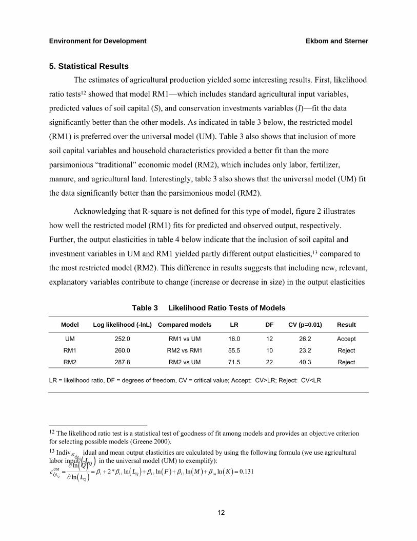
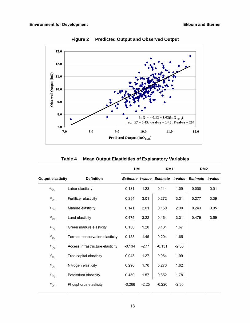
Acknowledging that R-square is not defined for this type of model, figure 2 illustrates
how well the restricted model (RM1) fits for predicted and observed output, respectively.
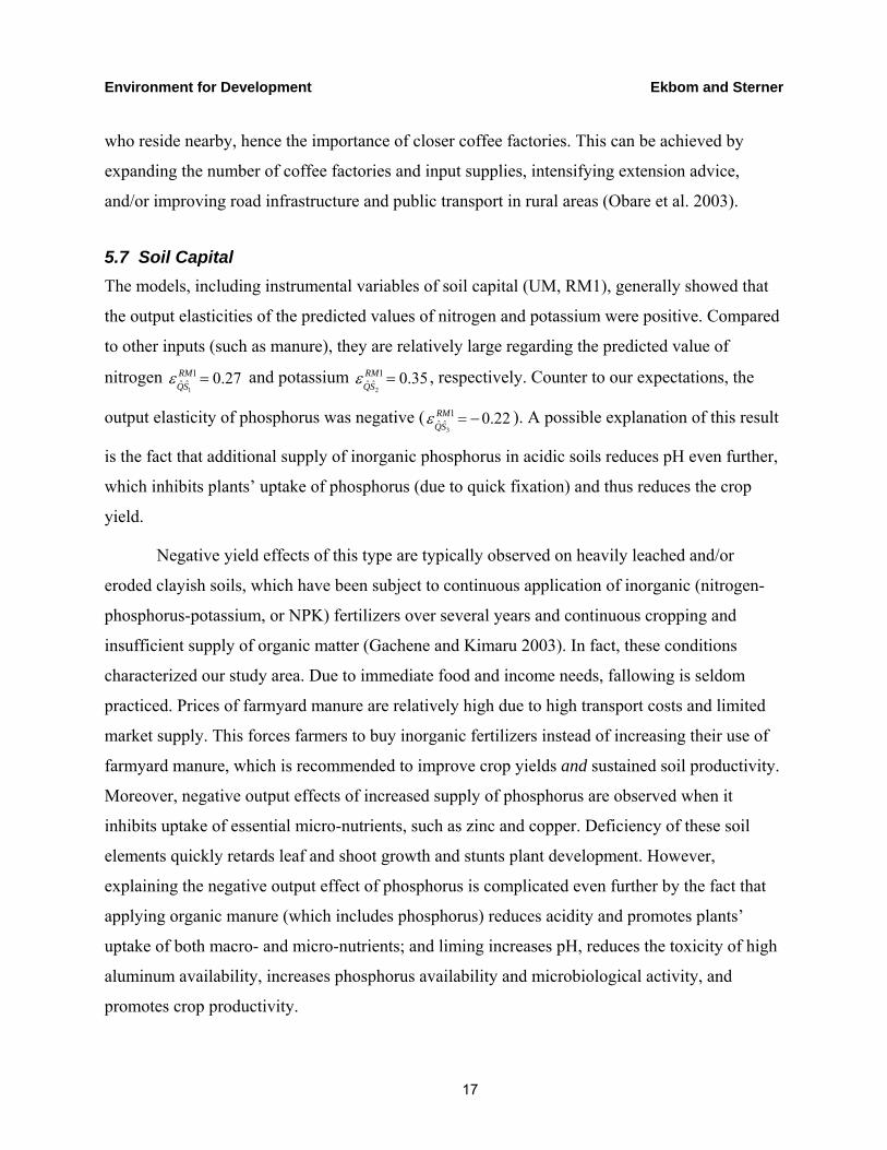
Further, the output elasticities in table 4 below indicate that the inclusion of soil capital and
investment variables in UM and RM1 yielded partly different output elasticities,13 compared to
the most restricted model (RM2). This difference in results suggests that including new, relevant,
explanatory variables contribute to change (increase or decrease in size) in the output elasticities
Table 3 Likelihood Ratio Tests of Models
Model Log likelihood (-lnL) Compared models LR DF CV (p=0.01) Result
UM 252.0 RM1 vs UM 16.0 12 26.2 Accept
RM1 260.0 RM2 vs RM1 55.5 10 23.2 Reject
RM2 287.8 RM2 vs UM 71.5 22 40.3 Reject
LR = likelihood ratio, DF = degrees of freedom, CV = critical value; Accept: CV>LR; Reject: CV<LR
12 The likelihood ratio test is a statistical test of goodness of fit among models and provides an objective criterion for selecting possible models (Greene 2000). 13 Indiv
ˆˆ
QQLε idual and mean output elasticities are calculated by using the following formula (we use agricultural
labor input ( )QL in the universal model (UM) to exemplify): ( )( ) ( ) ( ) ( ) ( )
ˆˆ 1 11 12 13 14
ˆln2* ln ln ln ln 0.131
lnQ
UMQQL
Q
QL F M K
Lε β β β β β
∂= = + + + + =
∂
Environment for Development Ekbom and Sterner
13
Figure 2 Predicted Output and Observed Output
lnQ = - 0.12 + 1.02(lnQRM 1)adj. R2 = 0.45; t-value = 14.3; F-value = 204
7.0
8.0
9.0
10.0
11.0
12.0
13.0
7.0 8.0 9.0 10.0 11.0 12.0
Predicted Output (lnQRM 1)
Obs
erve
d O
utpu
t (ln
Q)
Table 4 Mean Output Elasticities of Explanatory Variables
UM RM1 RM2
Output elasticity Definition Estimate t-value Estimate t-value Estimate t-value
ˆˆ
QQLε Labor elasticity 0.131 1.23 0.114 1.09 0.000 0.01
QFε Fertilizer elasticity 0.254 3.01 0.272 3.31 0.277 3.39
QMε Manure elasticity 0.141 2.01 0.150 2.30 0.243 3.95
QKε Land elasticity 0.475 3.22 0.464 3.31 0.479 3.59
1QIε Green manure elasticity 0.130 1.20 0.131 1.67
1QIε Terrace conservation elasticity 0.188 1.45 0.204 1.65
2QIε Access infrastructure elasticity -0.134 -2.11 -0.131 -2.36
3QIε Tree capital elasticity 0.043 1.27 0.064 1.99
1ˆ ˆQS
ε Nitrogen elasticity 0.290 1.70 0.273 1.62
2ˆ ˆQS
ε Potassium elasticity 0.450 1.57 0.352 1.78
3ˆ ˆQS
ε Phosphorus elasticity -0.266 -2.25 -0.220 -2.30

Environment for Development Ekbom and Sterner
14
produced by the traditional agricultural production function represented by RM2. Because we
were interested in the role and contribution of soil capital and (the quality of) soil conservation
investments, we focused on interpreting RM 1.
5.1 Agricultural Labor The mean output elasticity of labor was insignificant in all models and practically zero in
the most restricted model (RM2). Although statistically insignificant, this result points to the
abundance of labor (high per capita-to-land ratio) in the area and the low marginal productivity
of labor.
Interestingly, the regression results of the parameter estimates indicate a substitution
effect between agricultural labor and farmyard manure. Plotting the individual output elasticities
of labor against those of manure input (figure 3) confirmed the negative interaction effect
observed in all models (see appendix 4). This might be explained by specialization in farming
activities. Farmers who use little or no manure typically must increase their labor for cultivation,
Figure 3 Output Elasticity of Agricultural Labor and Manure Input (KSh)
Labour Output Elasticity and Manure Input (lnM)
Q L = 0.49 - 0.04(lnM)
adj. R2 = 0.78; t-value=-30.2;
-0.10
0.00
0.10
0.20
0.30
0.40
0.50
0.60
0.70
0.80
4.0 5.0 6.0 7.0 8.0 9.0 10.0 11.0
Manure Input (lnM)
Lab
our
Out
put E
last
icity
(Q
L)

Environment for Development Ekbom and Sterner
15
and vice versa. Interestingly, a similar negative relationship applied to labor and fertilizer.
Agronomic studies, which exclude labor input, will typically not pick up this result.
5.2 Chemical Fertilizer and Manure
The output elasticities of chemical fertilizer and manure in table 4 and in the parameter estimates in appendix 4 indicated that they are both positively associated with crop output. This applied to all of the three estimated models and is in accord with the lion’s share of the economic literature on determinants of agricultural production in developing countries (see, e.g., Mundlak et al. 1997; Fulginiti and Perrin 1998, Sherlund et al. 2002). The output elasticity of fertilizer was relatively stable across the models, whereas the output elasticity of manure decreased to around 40 percent in the models, including soil capital and investments (UM and RM1).
5.3 Agricultural Land In the table of elasticities (table 4), we noted that the mean output elasticity of
agricultural land is generally higher than the other output elasticities. The output elasticity of
land was relatively stable across the models and did not change significantly as we restricted the
universal model. The individual elasticities indicated that households with smaller plots
generally have higher output per unit area. The theory on benefit from economies of scale
suggests that the opposite result would be expected. However, our result is plausible if farmers
intensify production as farms become smaller. Our result agreed with other studies in similar
settings (see, e.g., Heltberg 1998), which also reflected the intensification in land use currently
taking place in Kenya. Land fragmentation into smaller and smaller plots pushes farmers away
from their land and forces the remaining farmers to intensify their land use.
5.4 Green Manure Well-managed green manure is positively associated with crop output (
1
1ˆ 0.13RM
QIε = ). This
result concurs with other relevant studies (see, e.g., Onim et al. 1990; Raquet 1990; Peoples and
Craswell 1992; Fischler and Wortmann 1999; Mureithi et al. 1998, 2002, 2003). For example,
Mureithi et al. (1998, 2000) reported that farmers in Thika District, in Kenya’s central highlands,
significantly increase their maize yields after growing legumes in the soil. Similarly, Onyango et

Environment for Development Ekbom and Sterner
16
al. (2001) found positive effects on crop yield when legumes (as green manure) were
intercropped with maize in smallholder farms in Kenya’s western highlands.
Arguably, the positive elasticity of green manure is due to the positive effects that
legumes have on the soil’s chemical, biological, and physical properties. Several studies have
shown that cultivation and incorporation of legumes into the soil increases ground cover,
prevents soil loss, reduces weed infestation and plant diseases, prevents leaching, supplies
additional nitrogen, improves soil tilth and water infiltration, builds up soil fertility, and
enhances crop productivity (Yost and Evans 1988; Lal et al. 1991; Hudgens 2000; Gachene and
Kimaru 2003).
5.5 Soil Conservation Terraces The output elasticities showed that high-quality soil conservation terraces are positively
associated with crop output. Specifically, the output elasticity of terrace conservation for the
restricted model (RM1) was significant and relatively large (2
1ˆ 0.20RM
QIε = ). This positive
relationship corresponds with other results from the region (see, e.g., Kilewe 1987; Gachene
1995; Pagiola 1999; and Stephens and Hess 1999).
5.6 Access to Public Infrastructure Table 4 shows that a shorter distance to public infrastructure promotes agricultural output
(3
1ˆ 0.13RM
QIε = − ).14 The particular result, that closer distance to a coffee factory is associated with
higher output, is plausibly explained by the following factors: coffee factories provide essential
crop management advice and other information to farmers;15 coffee factories sell inputs
(insecticides and fertilizers) and offer credits of various types; and closer access may induce
farmers to change their crop composition in favor of higher-value crops. Due to the opportunity
cost of time for transport, closer factories provide the advice and inputs more cheaply to farmers
14 The result applies specifically to access to coffee factories. However, we obtained negative signs on the parameter estimates and negative output elasticities for all types of public infrastructure collected in the data set. 15 Staff at the coffee factories professionally assess the quality of delivered coffee and commonly provide information on how to improve productivity and detect and prevent pests (such as coffee berry disease).
Environment for Development Ekbom and Sterner
17
who reside nearby, hence the importance of closer coffee factories. This can be achieved by
expanding the number of coffee factories and input supplies, intensifying extension advice,
and/or improving road infrastructure and public transport in rural areas (Obare et al. 2003).
5.7 Soil Capital The models, including instrumental variables of soil capital (UM, RM1), generally showed that
the output elasticities of the predicted values of nitrogen and potassium were positive. Compared
to other inputs (such as manure), they are relatively large regarding the predicted value of
nitrogen 1
1ˆ ˆ 0.27RM
QSε = and potassium 2
1ˆ ˆ 0.35RM
QSε = , respectively. Counter to our expectations, the
output elasticity of phosphorus was negative (3
1ˆ ˆ 0.22RM
QSε = − ). A possible explanation of this result
is the fact that additional supply of inorganic phosphorus in acidic soils reduces pH even further,
which inhibits plants’ uptake of phosphorus (due to quick fixation) and thus reduces the crop
yield.
Negative yield effects of this type are typically observed on heavily leached and/or
eroded clayish soils, which have been subject to continuous application of inorganic (nitrogen-
phosphorus-potassium, or NPK) fertilizers over several years and continuous cropping and
insufficient supply of organic matter (Gachene and Kimaru 2003). In fact, these conditions
characterized our study area. Due to immediate food and income needs, fallowing is seldom
practiced. Prices of farmyard manure are relatively high due to high transport costs and limited
market supply. This forces farmers to buy inorganic fertilizers instead of increasing their use of
farmyard manure, which is recommended to improve crop yields and sustained soil productivity.
Moreover, negative output effects of increased supply of phosphorus are observed when it
inhibits uptake of essential micro-nutrients, such as zinc and copper. Deficiency of these soil
elements quickly retards leaf and shoot growth and stunts plant development. However,
explaining the negative output effect of phosphorus is complicated even further by the fact that
applying organic manure (which includes phosphorus) reduces acidity and promotes plants’
uptake of both macro- and micro-nutrients; and liming increases pH, reduces the toxicity of high
aluminum availability, increases phosphorus availability and microbiological activity, and
promotes crop productivity.
Environment for Development Ekbom and Sterner
18
In view of these facts, determining the specific reasons for the negative sign of the
phosphorus elasticity requires more site-specific soil sample data and further study.16
Nonetheless, the negative phosphorus elasticity points to a typical information problem
associated with poverty. As opposed to farmers in developed countries, the farmers in our study
area are deprived of three kinds of services.
First, they have no access to appropriate soil analysis and specific information on the
status of their soil capital (nutrient levels, etc.). The situation is characterized by asymmetric
information, where farmers typically lack formal (scientific) information about their soil
capital.17 On the other hand, they have practical knowledge gained from experience.
Second, the farmers do not have a wide choice of fertilizers appropriate to their farm-
specific agro-ecological conditions. The local fertilizer market offers only few varieties with
fixed proportions of the key nutrients. The farmers’ ability to choose among many varieties of
fertilizers and fine tune choices to fit their individual crop-specific requirements is severely
limited. The most common type of chemical fertilizer used in the study area is di-ammonium
phosphate with the typical NPK distribution18 of 20:20:0, calcium (Ca) ammonium nitrate with
the typical NPKCa distribution of 20:20:0:13, and to a lesser extent NPK 17:17:17. All of these
fertilizers have a relatively high phosphorus content and low-to-no potassium. Consequently, the
farmers contribute to lower soil pH, which is already low (acidic), and hence impede plant
growth.
Third, the farmers are dependent on sub-optimal advice. Besides neighbors and relatives,
they primarily obtain advice on agriculture and land use from two sources—local suppliers and
government extension agents. The suppliers usually have a local monopoly in supplying
agricultural physical inputs. According to the farmers and suppliers in the study area, the
16 Personal communication among Gete Zeleke, Charles Gachene, Frank Place, and Anna Tengberg. 17 The lack of scientific information is also relevant for crops, where farmers could benefit from plant-tissue analysis and interpretation (Gachene and Kimaru 2003). 18 The percentage distribution refers to P2O5 (inorganic phosphorus) and K2O (inorganic potassium). Hence, 20:20:0 corresponds to 20% N, 20% P2O5, ad 0% K2O, plus ballast. For conversion to percentage weight distribution, inorganic P = 0.436 x (P2O5); elemental K = 0.83 x (K2O).

Environment for Development Ekbom and Sterner
19
suppliers frequently give advice on how and when to use their products (e.g., chemical fertilizers,
pesticides, improved seeds) despite limited specific knowledge of an individual farmer’s soil and
agro-ecological conditions.
Although government extension agents can provide more reliable information than the
suppliers, they too lack specific information on which fertilizers would be appropriate for the
individual farmer. Due to limited geographical coverage, infrequent visits, and lack of farm-
specific information (from soil sample analysis, for example), the extension advice tends to be
rather general. Given these obstacles, the farmers cannot optimize their fertilizer input and crop
composition as in modern agriculture. The fact that all farmers in the study used inorganic
fertilizers (which lower pH) is an indication of their lack of information about enhanced soil
management and/or access to other inputs (e.g., lime) to improve soil fertility.
Assessing Kenya’s fertilizer consumption across time (presented in table 5), the
percentage shares of nitrogen, phosphorus, and potassium have been relatively stable. The
percentage share of phosphorus as part of total fertilizer consumption is very large (around 50
percent). Conversely, the share of potassium has remained at a low level (5–10 percent). In 2002,
it was only 2 percent. The relatively low share of potassium and the relatively high share of
phosphorus are surprising and somewhat counterintuitive, given the positive output elasticity of
potassium and the negative output elasticity of phosphorus.
Table 5 Fertilizer Consumption in Kenya, 1962–2002 (% Share of Total NPK Consumption)
1962 1972 1982 1992 2002
Nitrogen (N) 29% 35% 44% 47% 40%
Phosphorus (P) 62% 53% 49% 45% 58%
Potassium (K) 9% 12% 6% 8% 2%
Source: FAO, FAOSTAT Data Base, http://apps.fao.org/faostat/ (Rome: FAO, 2005).

Environment for Development Ekbom and Sterner
20
In view of our statistical findings and the increasing use of inorganic fertilizers in
Kenya19 on already acidic soils (which impedes soil nutrient uptake and optimal plant growth), it
is essential that Kenya’s fertilizer use and soil nutrient-output relationships be addressed in a
comprehensive policy analysis. It is also noticeable that very few farmers reported use of
buffering fertilizers, such as rock phosphate or lime, despite the potential to ameliorate acidic
soils and increase crop production (Rutunga et al. 1998).
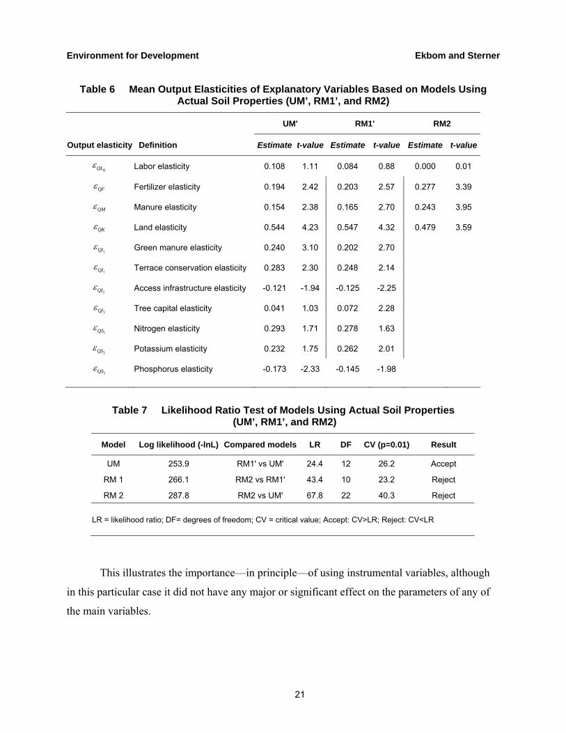
5.8 Sensitivity Analysis As a sensitivity test of our basic results, we estimated the productivity equation (1) using
the direct observed soil properties ( lS ), instead of the predicted values ( ˆlS ). As seen in tables 6
and 7 below, the differences compared with the earlier results are small and in no case
significant. Further, as indicated in table 7, it does not alter the previous outcome of the
likelihood ratio test.
However, one difference worth mentioning is the fertilizer elasticity. In UM’ and RM1’,
the fertilizer elasticity is around 0.20, which is somewhat (although not significantly) lower than
the corresponding elasticity for the simplest model RM2 with no variables on soil capital and soil
conservation investments. If one looked only at these OLS estimates, one might be tempted to
draw the conclusion that omitting soil properties had given us too high a value for the fertilizer
elasticity. However, the instrumental variable analysis showed that the elasticity is not affected at
all. This can be interpreted to mean that fertilizer application has a direct effect on yield together
with other variables and also an indirect long-run effect through improvements in soil status. The
latter connection is discussed in Ekbom (2007). Results may be biased if one does not take into
account that using the observed soil characteristics (Sl) in the regression gives a biased estimate,
and that some of the effect—that should be attributed to the fertilizer—can be wrongly attributed
to the soil characteristics.
19 Although Kenya’s total consumption of inorganic fertilizer is low compared to developed countries, consumption of NPK fertilizer has increased rapidly over the last 40 years. In 1961, Kenya’s total consumption of NPK fertilizer was 1,100 metric tons. In 2002, it had increased to 143,000 metric tons (FAO, 2005).
Environment for Development Ekbom and Sterner
21
Table 6 Mean Output Elasticities of Explanatory Variables Based on Models Using Actual Soil Properties (UM’, RM1’, and RM2)
UM' RM1' RM2
Output elasticity Definition Estimate t-value Estimate t-value Estimate t-value
QQLε Labor elasticity 0.108 1.11 0.084 0.88 0.000 0.01
QFε Fertilizer elasticity 0.194 2.42 0.203 2.57 0.277 3.39
QMε Manure elasticity 0.154 2.38 0.165 2.70 0.243 3.95
QKε Land elasticity 0.544 4.23 0.547 4.32 0.479 3.59
1QIε Green manure elasticity 0.240 3.10 0.202 2.70
1QIε Terrace conservation elasticity 0.283 2.30 0.248 2.14
2QIε Access infrastructure elasticity -0.121 -1.94 -0.125 -2.25
3QIε Tree capital elasticity 0.041 1.03 0.072 2.28
1QSε Nitrogen elasticity 0.293 1.71 0.278 1.63
2QSε Potassium elasticity 0.232 1.75 0.262 2.01
3QSε Phosphorus elasticity -0.173 -2.33 -0.145 -1.98
Table 7 Likelihood Ratio Test of Models Using Actual Soil Properties (UM’, RM1’, and RM2)
Model Log likelihood (-lnL) Compared models LR DF CV (p=0.01) Result
UM 253.9 RM1' vs UM' 24.4 12 26.2 Accept
RM 1 266.1 RM2 vs RM1' 43.4 10 23.2 Reject
RM 2 287.8 RM2 vs UM' 67.8 22 40.3 Reject
LR = likelihood ratio; DF= degrees of freedom; CV = critical value; Accept: CV>LR; Reject: CV<LR
This illustrates the importance—in principle—of using instrumental variables, although
in this particular case it did not have any major or significant effect on the parameters of any of
the main variables.

Environment for Development Ekbom and Sterner
22
Finally, all estimates of the translog restrictions (linear homogeneity and symmetry)
imposed in the models were found to be statistically insignificant. This indicates that the
restrictions did not introduce any major distortions in the suggested models.
6. Summary and Conclusions Our study has methodological, empirical, and policy results. Starting with
methodological results, we showed that integrating traditional economics and soil science is
valuable in this area of research. Omitting key variables in the analysis, such as measures of soil
capital, can cause omitted-variables bias, since farmers’ choices of inputs depend both on the
quality and status of the soil capital and on other economic conditions, such as availability and
cost of labor, fertilizers, and other inputs.
We complemented a traditional economic-production function model (including labor,
fertilizers, manure, and land) with specific soil properties, quality measures of soil and water
conservation investments, and other variables related to extension advice, access to public
infrastructure, and capital. Based on econometric analysis of data from individual farmer
interviews and soil sample data from Kenya’s central highlands, comparison of a universal
model (including all potentially relevant variables) and two restricted models yielded several
useful results.
First, major soil nutrients are important explanatory factors: nitrogen and potassium
increase output significantly, whereas higher phosphorus levels are actually detrimental to
output. This emphasizes the importance of ensuring adequate fertilizer policies that are adjusted
to local biophysical conditions and access to a wide choice of fertilizers in local markets.
Second, introduction of soil properties is associated with a decrease in the output elasticities of
farmyard manure. Exclusion of soil properties and soil conservation technologies introduces the
risk of biased coefficients of the other variables. Third, only the output elasticity of land
contributes more to output than nitrogen and potassium. The output elasticity of fertilizer is
relatively smaller. This underscores the importance of including soil capital in economic
analyses of agricultural output. Our sensitivity analysis further showed that our results are fairly
robust.

Environment for Development Ekbom and Sterner
23
A fourth result is that soil conservation technologies, such as terraces and green manure,
contribute to increased agricultural output even in models that also include soil properties and
chemical fertilizers. Given the policy debate on the impact (and usefulness) of government
subsidies on soil conservation, our results suggest that soil conservation investments contribute
to increasing farmers’ output. Consequently, government support for appropriate soil
conservation investments (green manure and terraces) not only helps arrest soil erosion, it also
helps farmers increase food production and reduce food insecurity. A final result is that since the
biophysical variables are important to explaining agricultural output, traditional economic
analyses need to reconsider the opportunities associated with greater integration of soil capital
and investments in land, among the explanatory variables.
Two central policy conclusions arise from this study. First, while fertilizers are generally
beneficial, their application is a complex art and more is not necessarily better: negative
phosphorus elasticities indicate that applying more potassium to these soils may in fact reduce
crop yield. In modern agriculture, it is standard practice to test soil properties on individual plots
in order to select the appropriate fertilizer in appropriate amounts and proportions. This practice
would be truly beneficial to Kenya’s agricultural production as well. Although farmers in many
instances possess vast local soil knowledge (Winklerprins 1999), they need to be able to combine
this knowledge with scientific information on soil capital and have better access to research-
based agricultural extension services.
Second, farmers and extension agents currently lack the means and the specific
knowledge necessary to pursue optimal agriculture, i.e., crop cultivation that is highly productive
and profitable and maintains soil capital across time. There is a need to strengthen the links to the
applied research and increase the use of integrated soil and land-use assessment based on
farmers’ knowledge, experiences, needs, preferences, and scientific knowledge. Relevant
research-based services which could be offered to farmers include formal soil-sample analysis,
expert judgment on optimal farming systems and land use, farm-specific soil mapping, plant-
tissue analysis, etc. We argue that the government has a special responsibility to provide these
opportunities in rural areas. One might argue, too, that if yields can be increased or risk of crop
failure reduced by better use of soil testing (and thus better informed fertilizer selection), then the

Environment for Development Ekbom and Sterner
24
market should start offering such services—soil testing combined with increased fertilizer supply
and extension advice.
Currently, however, these services are not offered by anyone at a significant level due to
a combination of several factors. The technical (or chemical) issues are highly complex and can
be difficult to communicate to farmers who have insufficient knowledge in this area. There is
asymmetric information between farmers and the private sector, which potentially could offer
soil and land-management services. Thin markets, which might offer farm-specific services,
often have suppliers with virtual monopolies of inputs at the local level and high investment risks
for private companies. From the farmers’ point of view, demand for soil sample analysis does
not occur naturally or easily, arguably due to poverty, risk aversion, and high discount rates.
Since practical experience and extension advice are lacking, the farmers are also uncertain or
unaware of the opportunities associated with soil management based on soil sample analysis,
which would complement their own knowledge and experiences. For all these reasons, it seems
appropriate that the government should, at least initially, take the lead in this area by speeding up
provision of farm-specific soil assessment, services for enhanced soil management, and facilitate
development of markets for it.

Environment for Development Ekbom and Sterner
25
References
Ackello-Ogutu, Christopher, Quirino Paris, and William A. Williams. 1985. “Testing a von Liebig Crop Response Function against Polynomial Specifications,” American Journal of Agricultural Economics 67(4)” 873–80.
Barrett, Christopher B., Alice Pell, David Mbugua, et al. 2004. “The Interplay between Smallholder Farmers and Fragile Tropical Agro-Ecosystems in the Kenyan Highlands.” Working Paper Series 8, no. 26. Social Science Research Network, online source. http://ssrn.com/abstract=601270. Accessed May 2, 2008.
Barrett, Scott. 1997. “Microeconomic Responses to Macroeconomic Reforms: The Optimal Control of Soil Erosion.” In The Environment and Emerging Development Issues, vol. 2, edited by Partha Dasgupta and Karl-Göran Mäler. Oxford: Clarendon Press.
Berck, Peter, and Gloria Helfand. 1990. “Reconciling the von Liebig and Differentiable Crop Production Functions,” American Journal of Agricultural Economics 72(4): 985–96.
Berck, Peter, Jacqueline Geoghegan, and Stephen Stohs. 2000. “A Strong Test of the von Liebig Hypothesis,” American Journal of Agricultural Economics 82(4): 948–55.
Berndt, Ernst R., and Laurits R. Christensen. 1974. “Testing for the Existence of a Consistent Aggregate Index of Labor Inputs,” American Economic Review 64(3): 391–404.
Byiringiro, Fidele, and Thomas Reardon. 1996. “Farm Productivity in Rwanda: Effects of Farm Size, Erosion, and Soil Conservation Investments,” Agricultural Economics 15 (2): 127–36.
Carrasco-Tauber, Catalina, and L. Joe Moffitt. 1992. “Damage Control Econometrics: Functional Specification and Pesticide Productivity,” American Journal of Agricultural Economics 74(1): 158–62
Carter, Michael R. 1984. “Identification of the Inverse Relationship between Farm Size and Productivity: An Empirical Analysis of Peasant Agricultural Production,” Oxford Economic Papers 36 (1): 131–45.
Cohen, Matthew J., Mark T. Brown, and Keith D. Shepherd. 2006. “Estimating the Environmental Costs of Soil Erosion at Multiple Scales in Kenya Using Energy Synthesis,” Agriculture, Ecosystems and Environment 114(2–4): 249–69.

Environment for Development Ekbom and Sterner
26
Christensen, Laurits R., Dale W. Jorgenson, Lawrence J. Lau. 1973. “Transcendental Logarithmic Production Frontiers,” Review of Economics and Statistics 55(1): 28–45.
Deolalikar, Anil B., and Wim P. M. Vijverberg. 1987. “A Test of Heterogeneity of Family and Hired Labor in Asian Agriculture,” Oxford Bulletin of Economics and Statistics 49(3): 291–305.
Ekbom, Anders, 2007. “Determinants of Soil Capital in Kenya.” In “Economic Analysis of Soil Capital, Land Use and Agricultural Production in Kenya.” PhD diss. Economic Studies, Department of Economics, University of Gothenburg, Sweden.
Ekbom, Anders, and Mira Ovuka. 2001. “Farmers’ Resource Levels, Soil Properties and Productivity in Kenya’s Central Highlands.” In Sustaining the Global Farm: Selected Scientific Papers from the 10th International Soil Conservation Organization Meeting, ed. D.E. Stott, R.H. Mohtar, and G.C. Steinhardt, 682-687. West Lafayette, IN: Purdue University and International Soil Conservation Organization.
FAO (Food and Agriculture Organization of the United Nations). 2005. “FAOSTAT Data Base.” Online source. http://apps.fao.org/faostat/.
Fischler, M., and C.S. Wortmann. 1999. “Green Manure for Maize-Bean Systems in Eastern Uganda: Agronomic Performance and Farmers’ Perceptions,” Agroforestry Systems 47(1–3): 123–38.
Frank, Michael D., Bruce R. Beattie, and Mary E. Embleton. 1990. “A Comparison of Alternative Crop Response Models,” American Journal of Agricultural Economics 72(3): 597–603.
Fulginiti, Lilyan E., and Richard K. Perrin. 1998. “Agricultural Productivity in Developing Countries,” Agricultural Economics 19(1–2): 45–51.
Gachene, Charles K.K. 1995. “Effects of Soil Erosion on Soil Properties and Crop Response in Central Kenya.” PhD diss., no. 22. Department of Soil Sciences, Swedish University of Agricultural Sciences, Uppsala, Sweden.
Gachene, Charles K.K., Nicholas Jarvis, H. Linner, J.P. Mbuvi. 1997. “Soil Erosion Effect on Soil Properties in a Highland of Central Kenya,” Soil Sciences Society of America Journal 61 (X): 559–64.
Environment for Development Ekbom and Sterner
27
Gachene, Charles K.K., J.P. Mbuvi, Nicholas Jarvis, and H. Linner. 1998. “Maize Yield Reduction Due to Erosion in a High Potential Area of Central Kenya Highlands,” African Crop Science Journal 6 (1): 29–37.
Gachene, Charles K.K., and Gathiru Kimaru. 2003. Soil Fertility and Land Productivity: A Guide for Extension Workers in the Eastern Africa Region. Technical Handbook, no. 30. RELMA Technical Handbook Series. Nairobi, Kenya: RELMA (Regional Land Management Unit) Publications and Sida (Swedish International Development and Cooperation Agency. http://www.worldagroforestry.org/sites/relma/Relmapublications/PDFs/TH30%20screen%20Quality.pdf. Accessed May 2, 2008.
Gerdin, Anders. 2002. “Productivity and Economic Growth in Kenyan Agriculture, 1964–1996,” Agricultural Economics 27(1): 7–13.
Greene, William H. 2000. Econometric Analysis. 4th ed. Upper Saddle River, NJ: Prentice-Hall.
Guilkey, David K., C.A. Knox Lovell, and Robin C. Sickles. 1983. “A Comparison of the Performance of Three Flexible Functional Forms,” International Economic Review 24(3): 591–616.
Hartemink, Alfred E., R.J. Buresh, P.M. van Bodegom, A.R. Braun, Bashir Jama, and B.H. Janssen. 2000. “Inorganic Nitrogen Dynamics in Fallows and Maize on an Oxisol and Alfisol in the Highlands of Kenya,” Geoderma 98(1–2): 11–33.
Heltberg, Rasmus. 1998. “Rural Market Imperfections and the Farm Size-Productivity Relationship: Evidence from Pakistan,” World Development 26(10): 1807–1026.
Hudgens, R.E. 2000. “Sustaining Soil Fertility in Africa: The Potential for Legume Green Manures: Soil Technologies for Sustainable Smallholder Farming Systems in East Africa.” Proceedings of the 15th Conference of the Soil Science Society of East Africa, Nanyuki, Kenya, August 19–23, 1996, 63–78.
Jacoby, Hanan G. 1992. “Productivity of Men and Women and the Sexual Division of Labor in Peasant Agriculture of the Peruvian Sierra,” Journal of Development Economics 37(1–2): 265–87.
———. 1993. “Shadow Wages and Peasant Family Labor Supply: An Econometric Application to the Peruvian Sierra,” Review of Economic Studies 60: 903–21.
Environment for Development Ekbom and Sterner
28
Kilewe, A. M. 1987. “Prediction of Erosion Rates and the Effects of Topsoil Thickness on Soil Productivity.” PhD diss. Department of Soil Science, University of Nairobi, Kenya.
Lal, Rattan, E. Reignier, W.M. Edwards, and R. Hammond. 1991. “Expectations of Cover Crops for Sustainable Agriculture.” In Cover Crops for Clean Water, ed. W. M. Hargrove, 1–11. Ankeny, IA: Soil and Water Conservation Society.
Mundlak, Yair, Don Larson, and Ritz Butzer, 1997. “The Determinants of Agricultural Production: A Cross-Country Analysis.” Policy Research Working Paper Series, no. 1827. Washington, DC: World Bank, Development Research Group.
Mureithi, J.G., C.K.K. Gachene, H.M. Saha, and E. Dyke. 1998. “Incorporation of Green Manure Legumes in Smallholder Farming Systems in Kenya: Achievements and Current Activities of the Legume Screening Network. In Agrobiological Management of Soils and Cropping Systems, ed. F. Rasolo and M. Raunet, 443–54. Montpelier, France: Grad.
Mureithi, J.G., P. Mwaura, and C. Nekesa. 2002. “Introduction of Legume Cover Crops to Smallholder Farms, Gatanga, Central Kenya.” In Participatory Technology Development for Soil Management by Smallholders in Kenya, ed. J.G. Mureithi, C.K.K. Gachene, F.N. Muyekho, M. Onyango, L. Mose, and O. Magenya, 153–164. Nairobi, Kenya: Kenya Agricultural Research Institute (KARI).
Mureithi, J.G., Charles K.K. Gachene, and J. Ojiem. 2003. “The Role of Green Manure Legumes in Smallholder Farming Systems in Kenya,” Tropical and Subtropical Agroecosystems 1(2–3): 57–70.
Nkonya, Ephraim, John Pender, Pamela Jagger, Dick Sserunkuuma, Crammer Kaizzi, and Henry Ssali. 2004. “Strategies for Sustainable Land Management and Poverty Reduction in Uganda.” Research Report 133. Washington, D.C.: International Food Policy Research Institute (IFPRI).
Obare, G.A., S.W. Omamo, and J.C. Williams. 2003. “Smallholder Production Structure and Rural Roads in Africa: The Case of Nakuru District, Kenya,” Agricultural Economics 28(3): 245–54
Okalebo, J.R., K.W. Gathua, and P.L. Woomer. 1993. Laboratory Methods of Soil and Plant Analyses: A Working Manual. Technical Publication, no. 1. Nairobi, Kenya: Soil Science Society of East Africa.
Onyango, Ruth M.A., Teresa K. Mwangi, John M. N’geny, Emily Lunzalu, and Joseph K. Barkutwo. 2001. “Effect of Relaying Green Manure Legumes on Yields of Intercropped
Environment for Development Ekbom and Sterner
29
Maize in Smallholder Farms of Trans Nzoia District, Kenya.” Proceedings from the 7th Eastern and Southern Africa Regional Maize Conference, Kitale, Kenya, February 11–15, 2001, 330–34.
Onim, J.F.M., M. Mathuva, K. Otieno, and H.A. Fitzhugh. 1990. “Soil Fertility Changes and Response of Maize and Beans to Green Manures of Leucaena, Sesbania, and Pigeonpea,” Agroforestry Systems 12(2): 197–215.
Ovuka, Mira, and Sven Lindqvist. 2000. “Rainfall Variability in Murang’a District, Kenya: Meteorological Data and Farmers’ Perception,” Geografiska Annaler, Series A: Physical Geography, 82(1): 107–119.
Ovuka, Mira. 2000. “Effects of Soil Erosion on Nutrient Status and Soil Productivity in the Central Highlands of Kenya.” PhD diss. Department of Physical Geography, Earth Sciences Center, University of Gothenburg, Sweden.
Pagiola, Stefano. 1999. Economic Analysis of Incentives for Soil Conservation. In Incentives in Soil Conservation: From Theory to Practice, ed. David W. Sanders, Paul C. Huszar, Samran Sombatpanit, and Thomas Enters. Oxford and New Delhi: World Association of Soil and Water Conservation and IBH Publishing Co. Ltd.
Rosenzweig, Cynthia, Ana Iglesias, Günther Fischer, Yuanhua Liu, Walter Baethgen, and James W. Jones. 1999. “Wheat Yield Functions for Analysis of Land-use Change in China,” Environmental Modeling and Assessment 4(2–3): 115–32.
Raquet, K. 1990. “Green Manuring with Fast-Growing Shrub Fallow in the Tropical Highlands of Rwanda: Ecofarming Practices for Tropical Smallholdings,” Tropical Agroecology 5: 55–80.
Rutunga, Venant, Kurt G. Steiner, Nancy K. Karanja, Charles K.K. Gachene, and Grégoire Nzabonihankuye. 1998. “Continuous Fertilization on Non-Humiferous Acid Oxisols in Rwanda a Plateau Central: Soil Chemical Changes and Plant Production,” Biotechnology, Agronomy, and Social Environment 2(2): 135–42.
Sherlund, Shane M., Christopher B. Barrett, and Akinwumi A. Adesina. 2002. “Smallholder Technical Efficiency Controlling for Environmental Production Conditions,” Journal of Development Economics 69(1): 85–101.
Simmons, Peter, and Daniel Weiserbs. 1979. “Translog Flexible Functional Forms and Associated Demand Systems,” American Economic Review 69(5): 892–901.

Environment for Development Ekbom and Sterner
30
Skoufias, Emmanuel. 1994. “Using Shadow Wages to Estimate Labor Supply of Agricultural Households,” American Journal of Agricultural Economics 76(2): 215–27.
Smaling, E.M.A., S.M. Nandwa, H. Prestele, R. Roetter, and F.N. Muchena.1992. “Yield Response of Maize to Fertilizers and Manure under different Agro-ecological Conditions in Kenya,” Agriculture, Ecosystems and Environment 41(1–2): 241–52.
Sombrok, W.G., H.M.H. Braun, and B.J.A. van der Pouw. 1982. “Exploratory Soil Map and Agro-Climatic Zone Map of Kenya,” Kenya Soil Survey, Exploratory Soil Survey Report, no. E1. Nairobi, Kenya: Ministry of Agriculture.
Stephens, William, and T. M. Hess. 1999. “Modelling the Benefits of Soil Water Conservation Using the PARCH Model—A Case Study from a Semi-arid Region of Kenya,” Journal of Arid Environments 41(3): 335–44.
Thomas, Donald B. 1995. Procedures for Evaluation of Soil and Water Conservation. Nairobi, Kenya: University of Nairobi, Department of Agricultural Engineering.
Thomas, Donald B., ed. 1997. Soil and Water Conservation Manual for Kenya. Nairobi: Ministry of Agriculture, Soil and Water Conservation Branch, and Livestock Development and Marketing.
Thomas, Michael F. 1994. Geomorphology in the Tropics: A Study of Weathering and Denudation in Low Latitudes. Hoboken, NJ: John Wiley and Sons.
Widawsky, David, Scott Rozelle, Songqing Jin, and Jikun Huang. 1998. “Pesticide Productivity, Host-Plant Resistance, and Productivity in China,” Agricultural Economics 19(1–2): 203–17.
Winklerprins, Antoinette M.G.A. 1999. “Local Soil Knowledge: A Tool for Sustainable Land Management,” Society & Natural Resources 12(2): 151–61.
Woomer, P.L., N. K. Karanja, and J.R. Okalebo. 1999. “Opportunities for Improving Integrated Nutrient Management by Smallholder Farmers in the Central Highlands of Kenya,” African Crop Science Journal 7(4): 441–54.
World Resources Institute. 2003. Geographic Dimensions of Well-Being in Kenya: Where Are the Poor? From Districts to Locations. Vol. 1. Nairobi, Kenya, and Washington, D.C.: Government of Kenya, Central Bureau of Statistics, and International Livestock Research Institute; and World Bank.

Environment for Development Ekbom and Sterner
31
Yost, R., and D. Evans. 1988. “Green Manure and Legume Covers in the Tropics.” HITAHR Research Series, no. 055. Mānoa: University of Hawaii, College of Tropical Agriculture and Human Resources, Hawaii Agricultural Experimental Station.

Environment for Development Ekbom and Sterner
32
Appendices
Appendix 1 Correlation Coefficients of Soil Properties
Variables S1 S2 S3 S4 S5 S6 S7 S8 S9 S10 S11
S1 Nitrogen 1 0.05 0.04 0.06 -0.12 -0.01 0.09 -0.03 -0.12 0.02 0.59 0.47 0.56 0.34 0.05 0.88 0.15 0.61 0.07 0.70 <.0001
S2 Potassium 1.00 0.10 0.12 -0.14 -0.02 0.08 -0.04 0.23 0.26 0.14 0.10 0.05 0.03 0.77 0.19 0.56 0.00 <.0001 0.03
S3 Phosphorus 1.00 0.07 -0.12 0.35 0.36 0.26 -0.10 0.36 0.06 0.26 0.06 <.0001 <.0001 <.0001 0.11 <.0001 0.31
S4 Sand 1.00 -0.88 0.00 -0.05 -0.06 0.14 0.00 0.15 <.0001 0.94 0.42 0.31 0.03 0.94 0.02
S5 Clay 1.00 -0.14 -0.07 -0.09 -0.11 -0.15 -0.23 0.02 0.29 0.17 0.07 0.02 0.00
S6 Calcium 1.00 0.53 0.74 -0.14 0.79 -0.05 <.0001 <.0001 0.03 <.0001 0.41
S7 pH 1.00 0.57 -0.19 0.59 -0.02 <.0001 0.00 <.0001 0.81
S8 Magnesium 1.00 -0.16 0.84 -0.16 0.01 <.0001 0.01
S9 Sodium 1.00 -0.10 0.00 0.12 0.95
S10 Cation Exchange Capacity 1.00 -0.03 0.64
S11 Carbon 1.00

Environment for Development Ekbom and Sterner
33
Appendix 2 Correlation Coefficients of Soil Conservation Quality Variables (1–12)
Nr. Variable 1 2 3 4 5 6 7 8 9 10 11 12
1 Cut-off drains 1 0.34 0.326 0.236 -0.044 0.09 0.111 0.19 0.41 0.214 0.201 0.446
<.0001 <.0001 0.0004 0.515 0.186 0.103 0.005 <.0001 0.002 0.003 <.0001
2 Crop cover 1 0.342 0.162 0.101 0.203 0.082 0.094 0.3 0.131 0.082 0.351
<.0001 0.017 0.136 0.003 0.229 0.166 <.0001 0.054 0.226 <.0001
3 Tillage practices 1 0.401 -0.08 -0.076 0.04 0.05 0.37 0.192 0.171 0.362
<.0001 0.237 0.261 0.56 0.465 <.0001 0.004 0.012 <.0001
4 Manure 1 0.121 0.081 0.072 0.056 0.45 0.134 0.23 0.285
0.074 0.236 0.289 0.41 <.0001 0.048 0.001 <.0001
5 Crop residue management 1 0.403 0.418 -0.012 0.06 -0.1 0.035 0.089
<.0001 <.0001 0.855 0.4 0.147 0.608 0.19
6 Mulching 1 0.433 0.05 0.1 0.063 0.046 0.182
<.0001 0.463 0.1 0.352 0.501 0.007
7 Green manure 1 0.041 0.16 0.153 0.041 0.128
0.55 0 0.024 0.545 0.059
8 Agro-forestry 1 0.17 0.183 0.642 0.315
0 0.007 <.0001 <.0001
9 Fodder management 1 0.266 0.262 0.357
<.0001 <.0001 <.0001
10 Grazing land management 1 0.249 0.157
0 0.021
11 Fuel wood 1 0.223
0.001
12 Terraces 1
Environment for Development Ekbom and Sterner
34
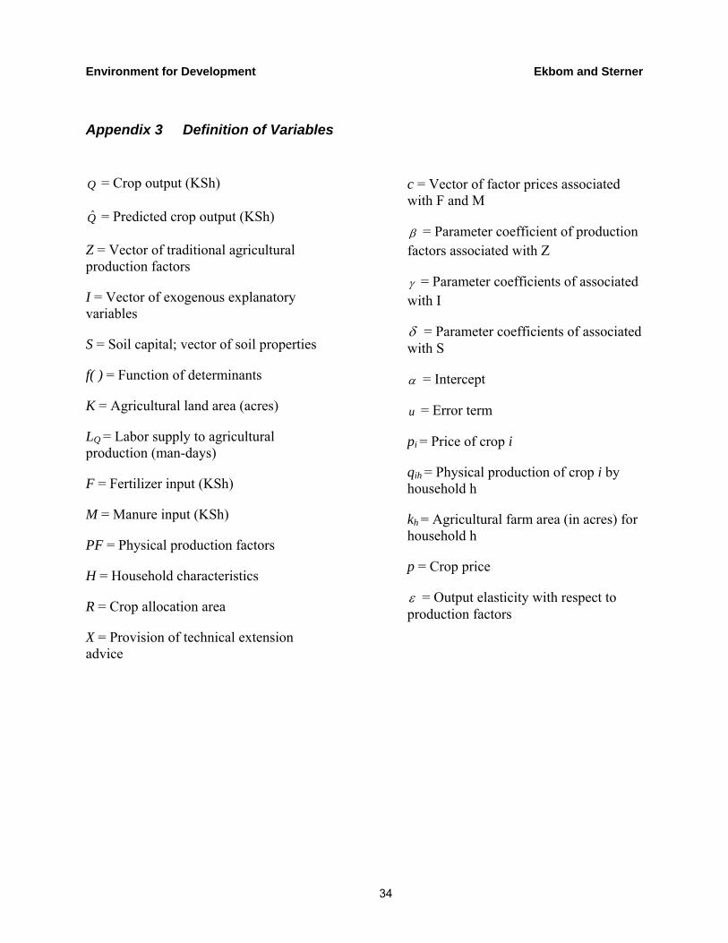
Appendix 3 Definition of Variables
Q = Crop output (KSh)
Q = Predicted crop output (KSh)
Z = Vector of traditional agricultural production factors
I = Vector of exogenous explanatory variables
S = Soil capital; vector of soil properties
f( ) = Function of determinants
K = Agricultural land area (acres)
LQ = Labor supply to agricultural production (man-days)
F = Fertilizer input (KSh)
M = Manure input (KSh)
PF = Physical production factors
H = Household characteristics
R = Crop allocation area
X = Provision of technical extension advice
c = Vector of factor prices associated with F and M
β = Parameter coefficient of production factors associated with Z
γ = Parameter coefficients of associated with I
δ = Parameter coefficients of associated with S
α = Intercept
u = Error term
pi = Price of crop i
qih = Physical production of crop i by household h
kh = Agricultural farm area (in acres) for household h
p = Crop price
ε = Output elasticity with respect to production factors
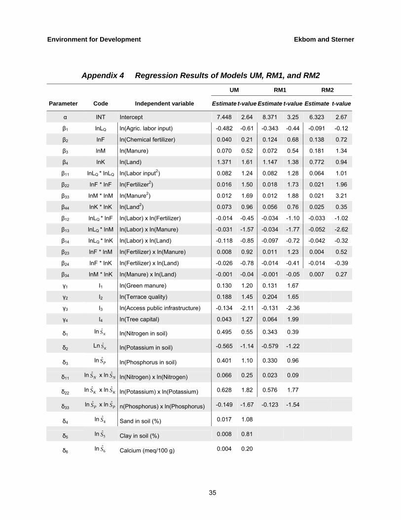
Environment for Development Ekbom and Sterner
35
Appendix 4 Regression Results of Models UM, RM1, and RM2
UM RM1 RM2
Parameter Code Independent variable Estimate t-value Estimate t-value Estimate t-value
α INT Intercept 7.448 2.64 8.371 3.25 6.323 2.67
β1 lnLQ ln(Agric. labor input) -0.482 -0.61 -0.343 -0.44 -0.091 -0.12
β2 lnF ln(Chemical fertilizer) 0.040 0.21 0.124 0.68 0.138 0.72
β3 lnM ln(Manure) 0.070 0.52 0.072 0.54 0.181 1.34
β4 lnK ln(Land) 1.371 1.61 1.147 1.38 0.772 0.94
β11 lnLQ * lnLQ ln(Labor input2) 0.082 1.24 0.082 1.28 0.064 1.01
β22 lnF * lnF ln(Fertilizer2) 0.016 1.50 0.018 1.73 0.021 1.96
β33 lnM * lnM ln(Manure2) 0.012 1.69 0.012 1.88 0.021 3.21
β44 lnK * lnK ln(Land2) 0.073 0.96 0.056 0.76 0.025 0.35
β12 lnLQ * lnF ln(Labor) x ln(Fertilizer) -0.014 -0.45 -0.034 -1.10 -0.033 -1.02
β13 lnLQ * lnM ln(Labor) x ln(Manure) -0.031 -1.57 -0.034 -1.77 -0.052 -2.62
β14 lnLQ * lnK ln(Labor) x ln(Land) -0.118 -0.85 -0.097 -0.72 -0.042 -0.32
β23 lnF * lnM ln(Fertilizer) x ln(Manure) 0.008 0.92 0.011 1.23 0.004 0.52
β24 lnF * lnK ln(Fertilizer) x ln(Land) -0.026 -0.78 -0.014 -0.41 -0.014 -0.39
β34 lnM * lnK ln(Manure) x ln(Land) -0.001 -0.04 -0.001 -0.05 0.007 0.27
γ1 I1 ln(Green manure) 0.130 1.20 0.131 1.67
γ2 I2 ln(Terrace quality) 0.188 1.45 0.204 1.65
γ3 I3 ln(Access public infrastructure) -0.134 -2.11 -0.131 -2.36
γ4 I4 ln(Tree capital) 0.043 1.27 0.064 1.99
δ1 ln ˆNS ln(Nitrogen in soil) 0.495 0.55 0.343 0.39
δ2 Ln ˆKS ln(Potassium in soil) -0.565 -1.14 -0.579 -1.22
δ3 ln ˆPS ln(Phosphorus in soil) 0.401 1.10 0.330 0.96
δ11 ln ˆNS x ln ˆ
NS ln(Nitrogen) x ln(Nitrogen) 0.066 0.25 0.023 0.09
δ22 ln ˆKS x ln ˆ
KS ln(Potassium) x ln(Potassium) 0.628 1.82 0.576 1.77
δ33 ln ˆPS x ln ˆ
PS n(Phosphorus) x ln(Phosphorus) -0.149 -1.67 -0.123 -1.54
δ4 ln 4S Sand in soil (%) 0.017 1.08
δ5 ln 5S Clay in soil (%) 0.008 0.81
δ6 ln 6S Calcium (meq/100 g) 0.004 0.20

Environment for Development Ekbom and Sterner
36
UM RM1 RM2
Parameter Code Independent variable Estimate t-value Estimate t-value Estimate t-value
δ7 ln 7S Soil pH (H2O) 0.105 1.03
δ8 ln 8S Magnesium (meq/100 g) -0.011 -0.38
δ9 ln 9S Sodium (meq/100 g) -0.014 -0.05
γ5 I5 Sex of household head (M=1; F=0) 0.011 0.09
γ6 I6 Age of household head (years) 0.006 0.99
γ7 I7 Education head (yrs.) -0.007 -0.46
γ8 I8 Livestock capital (KSh) 0.000 2.51
γ9 I9 Age of coffee trees (years) 0.006 0.22
γ10 I10 Family size (number of members) 0.030 1.32
R-square 0.47 0.43 0.31
Adjusted R-square 0.39 0.39 0.28
MSE 0.51 0.52 0.59

Environment for Development Ekbom and Sterner
37
Appendix 5a Estimates of Translog Restrictions on UM, RM1, and RM2
UM RM1 RM2
Restrictions Estimate t-value Estimate t-value Estimate t-value
β1+β2+β3+β4 = 1 7.5 1.21 -1.4 -0.21 -7.6 -1.10
β11 + 0.5*β12 + 0.5*β13 + 0.5*β34 = 0 94.8 1.11 -20.7 -0.22 -101.3 -1.07
0.5*β12 + β22 + 0.5*β23 + 0.5*β24 = 0 104.5 1.11 -39.6 -0.38 -134.5 -1.26
0.5*β13 + 0.5*β23 + β33 + 0.5*β34 = 0 45.2 0.45 -81.3 -0.76 -128.7 -1.19
0.5*β14 + 0.5*β24 + 0.5*β34 + β44 = 0 21.2 1.40 -1.6 -0.10 -13.1 -0.78
Appendix 5b Pearson Correlation Coefficients of Output Elasticities of Agricultural Production Variables
Output Output Elasticities
Elasticity Definition ˆQQL
ε QF
ε QM
ε QK
ε 1
ˆ ˆQSε
2ˆ ˆQS
ε 3
ˆ ˆQSε
ˆQQL
ε Labor elasticity 1.00 -0.58 -0.91 0.02 -0.04 -0.06 0.21
<.0001 <.0001 -0.6996 -0.5123 -0.3446 -0.0011
QFε Fertilizer elasticity 1.00 0.32 -0.09 -0.05 -0.07 -0.07
<.0001 -0.1492 -0.4004 -0.286 -0.3041
QMε Manure elasticity 1.00 -0.32 0.09 0.08 -0.24
<.0001 -0.1564 -0.1843 <.0001
QKε Land elasticity 1.00 -0.08 0.01 0.08
0.1884 0.9282 0.1971
1ˆ ˆQS
ε Nitrogen elasticity 1.00 -0.14 -0.14
0.0247 0.0312
2ˆ ˆQS
ε Potassium elasticity 1.00 0.15
0.018
3ˆ ˆQS
ε Phosphorus elasticity 1.00
n = 252

Environment for Development Ekbom and Sterner
38
Appendix 6 Regression Results of Models UM’, RM1’, and RM2
UM' RM1' RM2
Parameter Code Independent variable Estimate t-value Estimate t-value Estimate t-value
α INT Intercept 6.451 2.32 7.301 2.93 6.323 2.67
β1 lnLQ ln(Agric. labor input) -0.116 -0.15 0.011 0.01 -0.091 -0.12
β2 lnF ln(chemical fertilizer) 0.019 0.10 0.111 0.61 0.138 0.72
β3 lnM ln(Manure) 0.093 0.69 0.077 0.58 0.181 1.34
β4 lnK ln(Land) 1.004 1.23 0.801 1.02 0.772 0.94
β11 lnLQ * lnLQ ln(Labor input2) 0.043 0.69 0.049 0.80 0.064 1.01
β22 lnF * lnF ln(Fertilizer2) 0.015 1.38 0.014 1.35 0.021 1.96
β33 lnM * lnM ln(Manure2) 0.014 2.08 0.015 2.38 0.021 3.21
β44 lnK * lnK ln(Land2) 0.037 0.52 0.020 0.30 0.025 0.35
β12 lnLQ * lnF ln(Labor) x ln(Fertilizer) -0.007 -0.22 -0.029 -0.95 -0.033 -1.02
β13 lnLQ * lnM ln(Labor) x ln(Manure) -0.029 -1.48 -0.036 -1.86 -0.052 -2.62
β14 lnLQ * lnK ln(Labor) x ln(Land) -0.050 -0.38 -0.032 -0.25 -0.042 -0.32
β23 lnF * lnM ln(Fertilizer) x ln(Manure) 0.001 0.12 0.008 0.95 0.004 0.52
β24 lnF * lnK ln(Fertilizer) x ln(Land) -0.023 -0.70 -0.007 -0.21 -0.014 -0.39
β34 lnM * lnK ln(Manure) x ln(Land) 0.001 0.03 -0.002 -0.07 0.007 0.27
γ1 I1 ln(Green manure) 0.240 3.10 0.202 2.70
γ2 I2 ln(Terrace quality) 0.283 2.30 0.248 2.14
γ3 I3 ln(Access public infrastructure) -0.121 -1.94 -0.125 -2.25
γ4 I4 ln(Tree capital) 0.041 1.03 0.072 2.28
δ1 lnSN ln(Nitrogen) in soil) 0.023 0.03 -0.052 -0.06
δ2 lnSK ln(Potassium) in soil) -0.051 -0.64 -0.037 -0.46
δ3 lnSP ln(Phosphorus) in soil) -0.218 -1.42 -0.217 -1.42
δ11 lnSN x lnSN ln(Nitrogen) x ln(Nitrogen) -0.087 -0.33 -0.106 -0.41
δ22 lnSK x lnSK ln(Potassium) x ln(Potassium) 0.102 1.72 0.108 1.81
δ33 lnSP x lnSP ln(Phosphorus) x ln(Phosphorus) 0.015 0.49 0.025 0.81
δ4 lnS4 Sand in soil (%) 0.019 1.22
δ5 lnS5 Clay in soil (%) 0.008 0.77
δ6 lnS6 Calcium (meq/100 g) 0.014 0.60
δ7 lnS7 Soil pH (H2O) 0.113 1.14
δ8 lnS8 Magnesium (meq/100 g) -0.011 -0.38

Environment for Development Ekbom and Sterner
39
UM' RM1' RM2
Parameter Code Independent variable Estimate t-value Estimate t-value Estimate t-value
δ9 lnS9 Sodium (meq/100 g) -0.064 -0.24
γ5 I5
Sex of household head (M=1; F=0) 0.134 1.17
γ6 I6 Age of household head (years) -0.002 -0.39
γ7 I7
Education of household head (years)
-0.022 -1.65
γ8 I8 Livestock capital (KSh) 0.000 3.05
γ9 I9 Age of coffee trees (years) 0.001 0.25
γ10 I10
Family size (number of members) 0.035 1.59
R-square 0.47 0.42 0.31
Adjusted R-square 0.39 0.37 0.28
MSE 0.51 0.53 0.59
SSE 111.5 122 144.8
Appendix 7 Estimates of Translog Restrictions on UM’, RM1’, and RM2
UM' RM 1' RM 2
Restrictions Estimate t-value Estimate t-value Estimate t-value
β1+β2+β3+β4 = 1 6.9 1.08 -1.7 -0.24 -7.6 -1.10
β11 + 0.5*β12 + 0.5*β13 + 0.5*β34 = 0 82.9 0.94 -26.7 -0.28 -101.3 -1.07
0.5*β12 + β22 + 0.5*β23 + 0.5*β24 = 0 101.2 1.05 -40.5 -0.39 -134.5 -1.26
0.5*β13 + 0.5*β23 + β33 + 0.5*β34 = 0 41.0 0.40 -91.6 -0.84 -128.7 -1.19
0.5*β14 + 0.5*β24 + 0.5*β34 + β44 = 0 19.3 1.24 -2.5 -0.15 -13.1 -0.78