Production Forecasting of Petroleum Reservoir applying ...homepage.usask.ca/~mmg864/paper/RJ/RJ-2013-03.pdf · Production Forecasting of Petroleum Reservoir applying ... Accurate

International Journal of Computer Applications (0975 – 8887)

Volume 72– No.2, May 2013

23

Production Forecasting of Petroleum Reservoir applying

Higher-Order Neural Networks (HONN) with Limited

Reservoir Data

ABSTRACT

Accurate and reliable production forecasting is certainly a

significant step for the management and planning of the

petroleum reservoirs. This paper presents a new neural

approach called higher-order neural network (HONN) to

forecast the oil production of a petroleum reservoir. In

HONN, the neural input variables are correlated linearly as

well as nonlinearly, which overcomes the limitation of the

conventional neural network. Hence, HONN is a promising

technique for petroleum reservoir production forecasting

without sufficient network training data. A sandstone

reservoir located in Gujarat, India was chosen for simulation

studies, to prove the efficiency of HONNs in oil production

forecasting with insufficient data available. In order to reduce

noise in the measured data from the oil field a pre-processing

procedure that consists of a low pass filter was used. Also an

autocorrelation function (ACF) and cross-correlation function

(CCF) was employed for selecting the optimal input variables.

The results from these simulation studies show that the

HONN models have enhanced forecasting capability with

higher accuracy in the prediction of oil production.

Keywords: Production forecasting, reservoir performance, higher-order

neural network, higher-order synaptic operation.

1. INTRODUCTION An important phase in the field of petroleum reservoir

engineering is concerned with the forecasting of oil

production from the reservoir. This estimation of reserves in

the petroleum reservoirs involves massive investment of

money, time and technology under a wide range of operating

and maintenance scenarios such as well operations and

completion, artificial lift, workover, production, and injection

operations. A fairly precise estimation of oil quantity in the

reservoir is in demand; however, the rock and fluid properties

of the reservoirs are highly nonlinear and heterogeneous in

nature. Therefore, it is difficult to estimate an accurate

upcoming oil production. The oil production from a reservoir

depends on many static and dynamic parameters such as

porosity and permeability of rocks (static parameters), and

fluid saturation and pressure in the reservoir (dynamic

parameters). When these static and dynamic parameters are

available, the forecasting of oil production of a reservoir

would be more accurate. However, all the parameter data are

not always available. This limited data access from the oil

fields lessens the accuracy of production forecasting.

In the past, several forecasting methods have been developed

from decline curve analysis to soft computing techniques[1].

For the past few decades, artificial intelligence has been

extensively applied such as neural computing, fuzzy

inference systems and genetic algorithms in petroleum

industries because of its potential to handle the nonlinearities

and time-varying situations[2]. Neural networks (NN) is one of

the most attractive methods of artificial intelligence to cope

with the nonlinearities in production forecasting[3] as well as

in parameter estimation[4] due to its ability to learn and adapt

to new dynamic environments. Numerous researches have

shown successful implementation of NN in the field of oil

exploration and development such as pattern recognition in

well test analysis[5], reservoir history matching[6], prediction

of phase behavior[7], prediction of natural gas production in

the United States [8] and reservoir characterization[2] by

mapping the complex nonlinear input-output relationship. In

conventional NN model, each neural unit (neuron) performs

linear synaptic operation of neural inputs and synaptic

weights. Later, extensive researches on NN and applications

have been studied by Lee, et al.[9], Rumelhart and McClelland

[10], Giles and Maxwell[11], Gosh and Shin[12], Homma and

Gupta [13], Gupta, et al. [14], Redalapalli[15], Song[16], Tiwari[17].

The innovative neural structure embeds higher-order synaptic

operations (HOSO). Furthermore, the NN with HOSO

architecture was introduced and named as Higher-order neural

network (HONN)[14], [18]. The exclusive feature of HONN is

the expression of the correlation of neural inputs by

computing products of the inputs. It has been found that

HONN has significant advantages over conventional NN such

as faster training, reduced network size, and smaller

forecasting errors [15], [16], [17], [19].

This paper presents a new neural approach by employing

HONN to forecast oil production from an oil field reservoir

with limited parameter data: i) oil production data and ii) oil,

gas and water production data. Two case studies are carried

out to verify the potential of the proposed neural approach

with the limited available parameters from an oil field in

Gujarat, India. In case study-1, only one dynamic parameter

data, oil production data, are used for forecasting, whereas in

case study-2, three dynamic parameter data, oil, gas and water

production data are used for forecasting. A pre-processing

step is included for the preparation of neural inputs. The

details are explained in the succeeding sections.

Chithra Chakra N C College of Engineering

University of Petroleum & Energy Studies Dehradun, India

Ki-Young Song Department of Mechanical

Engineering The University of Tokyo

Japan

Deoki N Saraf College of Engineering

University of Petroleum & Energy Studies Dehradun, India

Madan M Gupta College of Engineering

University of Saskatchewan Saskatoon, Saskatchewan

Canada



24

2. Neural Networks (NN) and its Extension

to Higher-order Neural Networks

(HONN)

Neural networks (NN) are composed of several layers of

neural units (neurons): input layer, hidden layers and output

layer. A neural unit is structured mainly with two operations:

synaptic operation for weighting, and somatic operation for

mapping. In a conventional neural unit, the weighting process

is operated with linear correlation of neural inputs,

x_a=(x_0,x_1,x_2,…〖,x〗_n )∈ R^(n+1) (x_0 is bias), and

neural weights, w_a=(w_0,w_1,w_2,…〖,w〗_n )∈ R^(n+1)

(w_0=1). The linear correlation can be expressed

mathematically as

𝑣 = 𝑤0𝑥0 + 𝑤𝑖𝑥𝑖

𝑛

𝑖=1

(1)

However, in the nature, the correlation of neural inputs and

neural weights is not simply linear, but rather related

nonlinearly. This observation introduced a nonlinear (higher-

order) synaptic operation, and NN with the higher-order

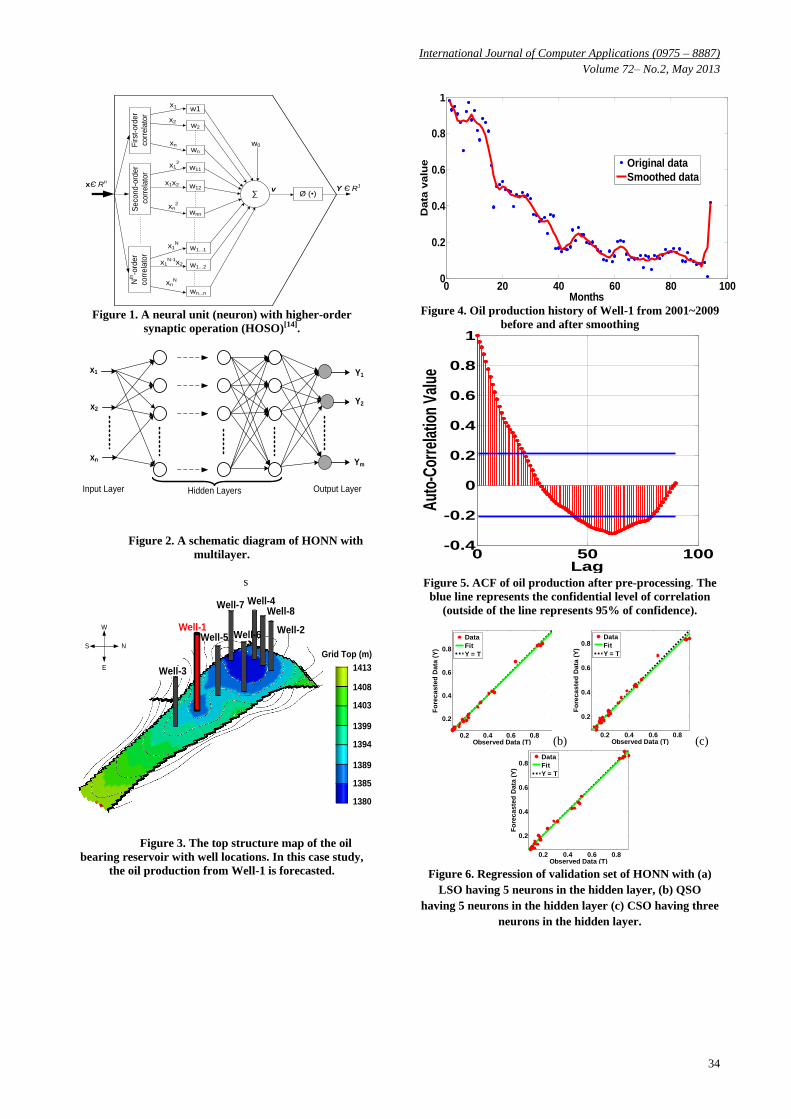
synaptic operation (HOSO) (see Figure 1) was developed and

named as higher-order neural networks (HONN)[19], [20],

[21]. HOSO of HONN embraces the linear correlation

(conventional synaptic operation) as well as the higher-order

correlation of neural inputs with synaptic weights (up to nth-

order correlation).

An nth order HOSO is defined as

𝑣 = 𝑤0𝑥0 + 𝑤𝑖1𝑥𝑖1

𝑛

𝑖1=1

+

+ 𝑤𝑖1𝑖2𝑥𝑖1

𝑥𝑖2

𝑛

𝑖2=𝑖1

𝑛

𝑖1=1

+ ⋯

+ … 𝑤𝑖1𝑖2…𝑖𝑁 𝑥𝑖1𝑥𝑖2

… … 𝑥𝑖𝑁

𝑛

𝑖𝑁 =𝑖𝑁−1

𝑛

𝑖2=𝑖1

𝑛

𝑖1 =1

(2)

and the somatic operation, which yields the neural output, is

defined as

𝑦 = ∅ 𝑣 (3)

In this paper, HOSO have been used up to third-order. The

first-order (conventional linear correlation), the second-order

and the third-order synaptic operations are called linear

synaptic operation (LSO), quadratic synaptic operation (QSO)

and cubic synaptic operation (CSO), respectively are applied.

The higher-order neural network (HONN) is illustrated in

Figure 2. HONN consists of multiple interconnected layers:

input layer, hidden layers and output layer. The input layer

conveys n number of input data to the first hidden layer. Each

hidden layer includes different number of neurons, and

consequently the output layer contains m neurons. The

number of the hidden layers and the number of neurons in

each hidden layer can be assigned after careful investigation

for different applications.

HONN is trained by an error based algorithm in which

synaptic weights (connection strength) are adjusted to

minimize the error between desired and neural outputs[19],

[20], [21]. Let x(k)∈R^n be the neural input pattern at time

step k=1,2…n corresponding to desired output y_d (k)∈R^1

and neural output y(k). The error of a pattern can be

calculated as

𝑒 𝑘 = 𝑦 𝑘 − 𝑦𝑑 𝑘 (4)

The overall error for an epoch E(k) is defined as

𝐸 𝑘 =1

2𝑒2 𝑘

(5)

The overall error (squared error) is minimized by updating the

weight matrix wa as

𝒘𝑎 𝑘 + 1 = 𝒘𝑎 𝑘 + ∆𝒘𝑎 𝑘 (6)

where the change in weight matrix is denoted by ∆wa (k)

which is proportional to the gradient of the error function E(k)

as

∆𝒘𝑎 𝑘 = −𝛼𝜕𝐸 𝑘

𝜕𝒘𝑎 𝑘

(7)

where α>0 is the learning rate which effects the performance

of the algorithm during the updating process. The details can

be found in the reference by Gupta et. al [14].

3. Model Performance Evaluation Criteria

Several statistical methods have been used to evaluate the

performance of neural networks in the literature. In these

studies, the following performance parameters are applied to

substantiate the statistical accuracy of the performance of

HONNs: root mean square error (RMSE) and mean absolute

percentage error (MAPE). These performance measurements

are commonly used evaluation criteria in assessing the model

performance. They indicate the deviation of prediction of

applied HONN models, and are defined as

Root mean square error (RMSE):

𝑅𝑀𝑆𝐸

= 1

𝑛 (𝑦𝑖

𝑜𝑏𝑠 − 𝑦𝑖𝑝𝑟𝑒𝑑

)2

𝑛

𝑖=1

(8)

Mean Absolute Percentage Error (MAPE):



25

𝑀𝐴𝑃𝐸 =100

𝑛

𝑦𝑖𝑜𝑏𝑠 − 𝑦𝑖

𝑝𝑟𝑒𝑑

𝑦𝑖𝑜𝑏𝑠

𝑛

𝑖=1

(9)

where 𝑦𝑜𝑏𝑠 is the observed data, 𝑦𝑝𝑟𝑒𝑑 is the predicted data,

and n is the number of data points.

Regression analysis is carried out for demonstrating the

HONN model performance during validation phase. The

model performance assessed by regression analysis is

illustrated using regression or parity plots. Using regression

plots one can assess how consistent is the forecasted data with

the observed data. It is considered that if the regression of a

model follows Y=T line more closely the model can perform

better prediction (see Figure 6), since the Y=T lines represent

the best fit.

In order to illustrate the consistency in performance

of HONN model towards forecasting the production data, we

have used two performance measurement metrics. The results

obtained using both metrics are different in their calculated

values, but the significance of each metrics is similar in

performance measurement of HONN model. Since the

production data used as neural input, preprocessed data and

raw data have different scales, it is preferable to use MAPE

for estimating the relative error [22].

4. Pre-Processing: Optimal Selection of

Input Variables

Before performing a prediction by HONN, it is

important and necessary to preprocess the available input data

because of two main reasons: i) noise reduction and ii) proper

selection of input variables. The measured oil production data

from the field include noise. It is not appropriate to use the

raw data for neural network training because NN requires

extremely low learning rates. A preprocessing of the raw

experimental production data was, therefore, incorporated in

all cases to minimize measurement errors. Moving average is

a type of low pass filter that transforms the time series

monthly production data into smooth trends. This filter does

weighted averaging of past data points in the time series

production data within the specified time span to generate a

smoothed estimate of a time series. The time span of moving

average depends on the analytical objectives of the problem.

For case studies, we used moving average filter with a time

span of five-points since it is found to be optimal for reducing

the random noise by retaining the sharpest step response

associated with production data. Moving average filter is the

simplest and perhaps optimal filter that can be used for time

domain signals as reported by Smith [23].

After noise reduction process, auto-correlation

analysis is carried out to find optimal input variables.

Determining the significant input variables is an important

task in the process of training HONN model for production

forecasting. A thorough understanding of dynamics in

petroleum reservoir is necessary to avoid missing key input

variables and prevent introduction of spurious input variables

that create confusion in training process. Currently, there is no

strict rule for the selection of input variables. Most of the

heuristic methods for selecting input variables are ad-hoc or

have experimental basis. In this paper, the significant input

variables are selected by employing auto-correlation function

(ACF) for single parameter data and cross-correlation

function (CCF) for multiple parameter data. These statistical

methods provide the correlation between different input

variables by identifying potentially influencing variables at

different time lags. The idea behind these statistical methods

is to investigate the dependence between the input variables.

ACF is a set of auto-correlation coefficients

arranged as a function of observations separated in time. It is a

common tool for assessing the pattern in time series

production data at numerous time lags. Consider the

observations 𝑥𝑡 and 𝑥𝑡+𝑘 ; t= 1, 2, …, n; then the

autocorrelation coefficient 𝑟(𝑘) at lagk can be calculated using

Eq.10

𝑟(𝑘) =1

𝑛 (𝑥𝑡 − 𝑥 )

𝑛−𝑘

𝑡=1

− 𝑥𝑡+𝑘 − 𝑥 ; 𝑥

= 𝑥𝑡

𝑛

𝑡=1

(10)

The CCF is a set of cross-correlation coefficients

arranged as a function of observations of one or more time

series data at different time steps (lag). Consider two time

series xt and yt, t= 1, 2, …, n; the time series yt may be

correlated to the past lags of time series xt and this can be

calculated using Eq. 11. Here rxy (k) is the cross-correlation

coefficient between xt and yt and k is the lag. This means

measurements in the variable y are lagging or leading those in

x by k time steps.

rxy (k)

=n (xt−x )(yt−y ) − xt yt

n xt2 − xt

2 n yt2 − yt

2

(11

)

The present study is based only on positive lags. The presence

of positive lagk between xt and yt indicates that the

relationship between these time series will be most significant

when the data in x at time t are related to data in y at time t+k.

In case study-1, ACF is applied to determine the optimal

input variables because only monthly oil production data is

used for forecasting. In case study-2, three parameter data, oil,

gas and water production data, are available as input and

hence CCF is used to determine the optimal input variables.

5. THE RESERVOIR UNDER STUDY The simulation studies are carried out with the

production data from a real oil field reservoir which has 94

months of production history. The oil field is located in south-

western part of Cambay Basin in Gujarat. This field consists

of total 8 oil producing wells. The structure of the field trends

NNW-SSE in direction and bounded by a fault on either side,

which separates the structure from the adjoining lows. The

reservoir structure is controlled by East-West trending normal

fault in the north, and it narrows down towards south. The

field composed of 3 sandstone layers (L-1, L-2, and L-3)

having varying thickness up to 25 m, and the layers are

separated by thin shales with thickness in the range of 1m to



26

2m. The graphical presentation of oil field reservoir for this

study is shown in Figure 3.

The initial reservoir pressure was recorded as 144

kg/cm2 at 1397m. The quantity of reserved oil inplace was

2.47MMt, and the cumulative oil production until September

2009 was 0.72MMt which is 29.1% of the inplace reserve and

64.5% of ultimate reserve. The field started producing oil

from February 2000 through Well-1 at a rate of 58m3/d and

December 2000 through Well-2. The initial reservoir pressure

recorded at Well-1 was 144.6 kg/cm2 at 1385m. From the

production performance, the cumulative productions of oil,

gas water from Well-1 till September 2009 are 0.156MMt,

8.1MMm3, and 7.2 Mm3, respectively. Later, other wells

(Well-3 ~ Well-8) were drilled and put on production in

different years until 2009.

The interest of this study is in forecasting the oil

production from the oldest well of the field, Well-1. Two

cases are studied for oil production forecasting using: i) only

oil production data and ii) oil, water and gas production data.

Tables 1. (a) and (b) present the raw and smoothed monthly

oil, gas and water productions ratios corresponding to each

maximum production values of Well-1 from 2001 to 2009.

For an efficient training for HONN, the monthly production

ratios were calculated using the maximum production of

products (3000 m3/month for oil, 150000 m3/month for gas,

and 1500 m3/month for water) through the 9 years production

history of Well-1.

5.1 Structure of HONN For this study, a number of design factors for HONN were

considered such as selection of neural structure (order of

synaptic operation), numbers of neurons and hidden layers.

Also, different mapping functions (somatic operation) were

selected after careful investigation in each layer: a sigmoidal

(hyperbolic tangent) function for hidden layers and a linear

function for the output layer.

Three synaptic operations, linear synaptic operation

(LSO), quadratic synaptic operation (QSO) and cubic synaptic

operation (CSO) were employed for this study. Only one

hidden layer was used since it resulted in the best output for

time sequence applications such as forecasting [17], and

different number of neurons (1~5) in the hidden layer were

applied. Each HONN model was run with learning rate of

0.01 and different initial synaptic weights. The learning rate

was dynamically updated by multiplying with 1.05 for

decreasing error and with 0.7 for increasing error. The pre-

processed data were divided into three segments for training,

testing and validation. The number of data sets used for

training and testing of HONN model for each case study

varied; however, last 16 months (month 78~94) data are used

to validate HONN models for case study. Each model was

performed for 200 epochs for training and testing, and then, a

validation was carried out.

The network was designed for prediction mode. If

the input to the network was production data at time t, then

the output is taken to at time t+1. During the network training,

the network output was compared with the production data at

time t+1 and the error was used to correct the synaptic

weights. This means that the network is used as a one-step-

ahead predictor. This is necessary for production forecasting.

5.2 Case Study-1

The monthly oil production ratios from month 1 to

month 94 were used for oil production forecasting as listed in

Table 1 a. In the pre-processing stage, the oil production ratio

data were smoothed using a five point moving average filter.

The smoothed oil production data are presented in Table 1 b.

The graphical representation of original oil production data

and smoothed data are shown in Figure 4. As seen in the

figure, the high peaks of the data were smoothed. After the

smoothing process, the auto-correlation of the oil production

data was calculated by auto-correlation function (ACF). The

ACF plot of oil production after smoothing is presented in

Figure 5. The ACF shows that the lags from lag0 to lag21

have some correlation within the 95% confidence level

(outside of the blue lines, positive region). From the ACF

plot, it was identified that lag1 and lag2 have the most

significant correlation which means that the input variables in

these lags are the optimal to train HONN. In view of above,

we trained HONN to forecast oil production based on three

scenarios:

1) using only lag1 (single lag1)

2) using only lag2 (single lag2)

3) using lag1 and lag2 (accumulated lag2)

1) HONN using Single Lag1

In scenario 1, first 51 months data were used for training

and next 26 months data for testing. The lag1 data presented

to HONN after pre-processing are given in Table 2. In this

table, input corresponds to oil productions rates from Well-1

and target corresponds to the oil production data that has been

advanced by one step. The regressions of the best HONN

models with LSO, QSO and CSO for the validation set of data

are presented in Figures 6. (a), (b), (c); respectively.

The simulation results from HONN model in terms

of RMSE and MAPE are show in Table 3. The selection

criteria for a better model are lower values of MAPE and

RMSE. From simulation results, the best model was HONN

with LSO having five neurons in the hidden layer. The

performance indices of best model shows HONN with LSO

resulted in MAPE = 13.86%. With CSO, MAPE =14.89% was

achieved with three neural units in the hidden layer, and

MAPE =15.98% was achieved with QSO having five neurons

in the hidden layer.

2) HONN using Single Lag2

For scenario 2, first 50 months data for training and

next 26 months data for testing were selected applying single

lag2 after pre-processing and the data were arranged as listed

in Table 4. In single lag2, the target data used for HONN are

advanced by 2 time steps.

Table 5 lists the simulation results using single lag2

from HONN models. The performance indices of the best

HONN model with LSO resulted in MAPE = 18.6. However,

the HONNs with QSO and CSO did not result in acceptable

outputs with single lag2. Parity plots are not included here for

brevity.

3) HONN using accumulated Lag2



27

For this scenario, accumulated lag2 (lag1 and lag2), the

input, train and test data are shown in Table 6. Input-1 and

Input-2 in Table 6 corresponds to oil production from Well-1

at time lag1 and time lag-2.

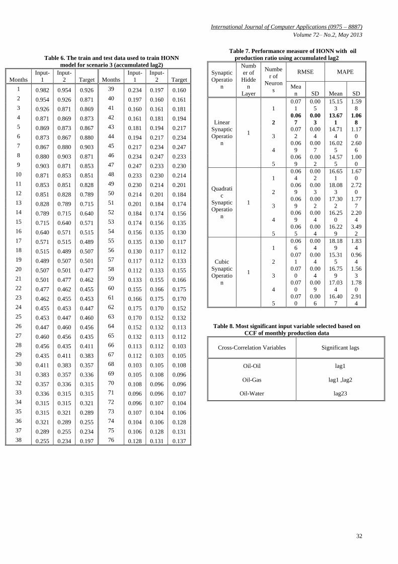
The simulation results using accumulated lag2 are

presented in Table 7. From this table it is seen that HONN

with LSO having two neurons in the hidden layer resulted in

MAPE = 13.671% and RMSE=0.067. These results are

comparable to those obtained in scenario1 but the standard

deviations are higher, meaning, thereby, that using lag2 in any

form does not help the predictions.

For case study-1, the overall performance measure

shows that HONN with LSO resulted in good performances

by yielding a stable value between the range of, RMSE =0.066~0.084 and 𝑀𝐴𝑃𝐸 = 13~18% with different

configurations of neurons in the hidden layer.

5.3 Case Study-2

For this simulation study, monthly oil, gas and

water production rates from Well-1 from September 2001 to

March 2009 were used for oil production forecasting. Table 1

a and b, present the monthly oil, gas and water production

data ratios for 94 months before and after smoothing.

This case study shows how additional input

parameters (gas and water production) influence the

performance of HONN model in forecasting oil production.

The production data were preprocessed by applying

smoothing process and cross-correlation. The smoothing

process was carried out by a moving averaging filter with five

sequence data points as discussed earlier. Oil, gas and water

production ratios, before and after smoothing, are graphically

presented in Figure 4 (oil), Figure 7.a (gas) and Figure 7.b

(water). After that, smoothed data were used to find cross-

correlation function (CCF) between three production data as

shown in Figure 8. The significant input variables were

determined using CCF by identifying the correlation between

oil and other components. It is observed from the CCF plot

that the correlations between oil and oil (auto-correlation), oil

and gas, oil and water are significant at lag1; lag1; and lag2,

and lag23, respectively (Table 8). A total of 4 input vectors

were identified for monthly oil production forecasting by

HONN model. The smoothed data from Table 1 b. were

arranged applying the lags obtained from the CCF plot as

presented in Table 8. Input1 represents the correlation of oil at

lag1, input 2 and input 3 refers to the correlation of oil with

gas production at lag1 and lag2, and input 4 represents the

correlation of oil with water production at lag23 (see Table 9

for the input and output data for this case).

Table 10 presents the results from HONN models

with its performance measure in terms of RMSE and MAPE

for different configurations of neurons in the hidden layer and

synaptic operation. In this case study, the best model resulted

in MAPE=15.13%, and RMSE=0.069 by HONN with QSO

having four neurons in the hidden layer.

6. PRODUCTION FORECASTING

Using the HONN, one-step-ahead production model, for

Well-1 in the Tarapur block of Cambay Basin, predictions

were made for 16 months (from February 2008 to September

2009 (i.e month 77 ~ 94) beyond the date used for model

development and its training. A comparison of the prediction

by the best HONN model with LSO using single lag1 with the

actual oil production is presented by Figure 9. As seen in this

model, the match is satisfactory for the first 13 months.

7. DISCUSSIONS

From the case studies, the performance evaluation

criteria indicates that the better oil production forecasting can

be achieved using HONN with LSO with only one input

parameter i.e. oil production data. In this study, the selection

of lag time is an important factor that influences the

forecasting results. Auto-correlation function (ACF) indicates

that the most significant lag for oil production forecasting

with only one parameter (oil production) is lag1, and HONN

with LSO yields the best forecasting oil production in this

case. Intuitively, it can be expected that QSO and CSO would

result in better outcome than that of LSO. However, this case

study comes up with opposite result. This can be explained by

recalling that only one input parameter (oil production), used

in case study-1, does not generate complex correlation with

target parameter (oil production to be predicted). Thus, in this

case, linear combination of synaptic operations could result in

better prediction. However, in case study-2, the three input

parameters, namely; oil, gas and water production rates may

generate nonlinearity and heterogeneity between input and

target parameters. In this case, the higher-order synaptic

operations, QSO and CSO, would be better suited to forecast

the oil production.

It is observed that the performance of HONN with

LSO in the case study-1 shows less MAPE than that in the

case study-2. One would expect that since gas and water

production rates are intimately connected with oil production

rate, case study-2 ought to have shown better match or less

MAPE. The contrary results may be attributed to the

possibility that the noise in gas and water production

measurements even after filtering may have overshadowed the

advantage gained by added input information. Additionally,

the number of input patterns in case study-1 is higher than that

in the case study-2. The reduction in the number of input

patterns for training HONN in the case study-2 is caused by

the number of lags. In the case study-2, the highest number of

lags is 23 which reduce the input pattern numbers as P – 23

where P is the number of initial input patterns. The patterns

for oil, gas and water productions are selected based on cross-

correlated pattern Overall, it can be inferred that for the

application of HONN for forecasting, the number of input

variables is one of the significant factors in determining the

order of synaptic operation.

Mean absolute percentage error (MAPE) is a

measure of uncertainty in forecasting of oil production from a

single well. A high value of 13 ~ 15% is indicative of lack of

enough input information to the HONN model. One important

information that is missing is clearly the well pressure

(bottom hole pressure). Another one is the presence of other

wells in its vicinity and their production pattern which, to

some extent, could have been reflected by the well pressure. It

may, therefore, be anticipated that if we were to use this

procedure for all the five wells in this reservoir, MAPE will

be reduced. Preliminary work on these lines indicates a

reduction by as much as 75% in the MAPE. This work will be

published at a future date when completed.



28

8. CONCLUSION

A new neural approach for forecasting oil

production using higher-order neural network (HONN) was

proposed in this paper. Two case studies were carried out with

the data from an oil field situated at Cambay basin, Gujarat,

India, to demonstrate the forecasting ability of HONN models.

The simulation study indicates that HONN has high

potential for application in oil production forecasting with

limited available input parameters of petroleum reservoirs.

The HONN methodology applied to forecasting of oil

production yielded 13.86 and 15.13 of MAPE in the two cases

examined. In order to achieve the MAPE, two pre-processing

procedures were found to be beneficial: i) noise reduction and

ii) selection of optimal input variables. In this study, a low

pass filtering process, a 5-point moving averaging filter, for

noise reduction was used. Auto-correlation function for single

input parameter and cross-correlation function for multiple

input parameters were employed to determine the most

significant correlation between the parameters. Considering

the limited available input parameters for forecasting, the

performance indicates that HONN has a high potential to

overcome this limitation. Also, for complicated input patterns,

such as in the cast study-2, the higher combination of the

input products reduces the computational cost, which yields

faster results.

9. ACKNOWLEDGMENTS

We thank Institute of Reservoir Studies, ONGC, India

for their support in providing field production data for this

work. The work of first author was financially supported by

Canadian Commonwealth Fellowship and University of

Petroleum and Energy Studies. The fourth author

acknowledges the fund provided by NSERC Discovery Grant.

The valuable comments and recommendations from the

reviewers are acknowledged.

10. REFERENCES

[1] D. Tamhane, P. M. Wong, F. Aminzadeh, and M.

Nikravesh, "Soft Computing for Intelligent Reservoir

Characterization," in SPE Asia Pacific Conference on

Integrated Modelling for Asset Management Yokohama,

Japan, 2000, pp. 1-11.

[2] S. D. Mohaghegh, "Recent Developments in Application

of Artificial Intelligence in Petroleum Engineering,"

Journal of Petroleum Technology, vol. 57, pp. 86-91,

2005.

[3] W. W. Weiss, R. S. Balch, and B. A. Stubbs, "How

Artificial Intelligence Methods Can Forecast Oil

Production," in SPE/DOE Improved Oil Recovery

Symposium, Tulsa, Oklahoma: Society of Petroleum

Engineers, 2002, pp. 1-16.

[4] F. Aminzadeh, J. Barhen, C. W. Glover, and N. B.

Toomarian, "Reservoir Parameter Estimation Using a

Hybrid Neural Network," Comput. Geosci., vol. 26, pp.

869-875, 2000.

[5] A. U. Al-Kaabi and W. J. Lee, "Using Artificial Neural

Networks To Identify the Well Test Interpretation Model

" SPE Formation Evaluation, vol. 8, pp. 233-240, 1993.

[6] C. Maschio, C. P. V. de Carvalho, and D. J. Schiozer, "A

New Methodology to Reduce Uncertainties in Reservoir

Simulation Models Using Observed Data and Sampling

Techniques," Journal of Petroleum Science and

Engineering, vol. 72, pp. 110-119, 2010.

[7] W. A. Habiballah, R. A. Startzman, and M. A. Barrufet,

"Use of Neural Networks for Prediction of Vapor/Liquid

Equilibrium K-Values for Light-Hydrocarbon Mixtures,"

SPE Reservoir Engineering, vol. 11, pp. 121-126, 1996.

[8] S. M. Al-Fattah and R. A. Startzman, "Predicting Natural

Gas Production Using Artificial Neural Network," in

SPE Hydrocarbon Economics and Evaluation

Symposium, Dallas, Texas: Society of Petroleum

Engineers, 2001, pp. 1-11.

[9] Y. C. Lee, G. Doolen, H. H. Chen, G. Z. Sun, T.

Maxwell, H. Y. Lee, and C. L. Giles, "Machine Learning

Using a Higher Order Correlation Network," Phys. D,

vol. 2, pp. 276 - 306, 1986.

[10] D. E. Rumelhart and J. L. McClelland, Parallel

Distributed Processing: Explorations in the

Microstructure of Cognition. Cambridge, MA: The MIT

Press, 1986.

[11] C. L. Giles and T. Maxwell, "Learning, Invariance, and

Generalization in High-Order Neural Networks," Applied

Optics, vol. 26, pp. 4972-4978., 1987.

[12] J. Gosh and Y. Shin, "Effcient Higher-Order Neural

Networks For Classification And Function

Approximation," International Journal of Neural

Systems, vol. 3, pp. 323-350., 1992.

[13] N. Homma and M. M. Gupta, "Superimposing Learning

for Backpropagation Neural Networks," Bulletin of

College of Medical Sciences, Tohoku University, vol. 11,

pp. 253-259, 2002.

[14] M. M. Gupta, L. Jin, and N. Homma, Static and Dynamic

Neural Networks: From Fundamentals to Advanced

Theory, 1 ed.: Wiley - IEEE Press, 2003.

[15] S. K. Redlapalli, "Development of Neural Units with

Higher-order Synaptic Operations and Their

Applications to Logic Circuits and Control Poblems," in

Department of Mechanical Engineering: University of

Saskatchewan, Canada, 2004.

[16] K.-Y. Song, M. M. Gupta, and D. Jena, "Design of An

Error-Based Robust Adaptive Controller," in Systems,

Man and Cybernetics, 2009. SMC 2009. IEEE

International Conference on, 2009, pp. 2386-2390.

[17] M. K. Tiwari, K. Y. Song, C. Chatterjee, and M. M.

Gupta, "River-flow Forecasting Using Higher-order

Neural Networks," Journal of Hydrologic Engineering,

vol. 17, pp. 1-12, 2012.

[18] Z.-G. Hou, K.-Y. Song, M. M. Gupta, and M. Tan,

"Neural Units with Higher-Order Synaptic Operations for

Robotic Image Processing Applications," Soft Comput.,

vol. 11, pp. 221-228, 2006.

[19] M. M. Gupta, N. Homma, Z.-G. Hou, A. M. G. Solo, and

I. Bukovsky, "Higher Order Neural Networks:

Fundamentals Theroy and Appplications," in Artificial

Higher-Order Neural Networks for Computer Science

and Engineeing: Trends for emerging Applications, M.

Zhang, Ed.: Information Science Reference, 2010, pp.

397-422.

[20] M. M. Gupta, "Correlative Type Higher-Order Neural

Units with Applications," in Automation and Logistics,

2008. ICAL 2008. IEEE International Conference, 2008,

pp. 715-718.

[21] M. M. Gupta and D. H. Rao, Neuro-Control Systems-

Theory and Applications: IEEE Neural Networks

Council, 1993.

[22] A. Azadeh, S. F. .Ghaderi, and S. Sohrabkhani,

"Forcasting Electrical Consumption by Integration of



29

Neural Network, Time Series and ANOVA," Applied

Mathematics and Computation, 2006.

[23] S. W. Smith, The Scientist and Engineer's Guide to

Digital Signal Processing, 1997.

Table 1 a. Ratio of monthly oil, gas and water production

to corresponding maximum production value of nine years

from Well-1.

Months Oil Gas Water Months Oil Gas Water

1 0.982 0.982 0.096 48 0.240 0.164 0.920

2 0.930 0.930 0.135 49 0.241 0.163 0.965

3 0.950 0.950 0.245 50 0.198 0.140 0.625

4 0.907 0.907 0.244 51 0.192 0.150 0.670

5 0.862 0.862 0.144 52 0.200 0.160 0.653

6 0.704 0.704 0.074 53 0.174 0.131 0.603

7 0.922 0.922 0.060 54 0.157 0.110 0.699

8 0.972 0.972 0.076 55 0.147 0.102 0.686

9 0.874 0.884 0.057 56 0.101 0.073 0.810

10 0.927 0.914 0.052 57 0.097 0.073 0.785

11 0.818 0.806 0.287 58 0.150 0.108 0.602

12 0.764 0.753 0.326 59 0.091 0.065 0.386

13 0.884 0.872 0.152 60 0.123 0.088 0.557

14 0.862 0.849 0.134 61 0.205 0.148 0.666

15 0.813 0.801 0.111 62 0.207 0.149 0.622

16 0.624 0.618 0.180 63 0.205 0.145 0.664

17 0.393 0.387 0.542 64 0.133 0.096 0.516

18 0.507 0.500 0.410 65 0.102 0.071 0.635

19 0.517 0.386 0.366 66 0.114 0.076 0.701

20 0.536 0.401 0.375 67 0.107 0.073 0.686

21 0.490 0.368 0.420 68 0.110 0.073 0.688

22 0.486 0.364 0.537 69 0.127 0.089 0.626

23 0.478 0.359 0.552 70 0.059 0.040 0.224

24 0.396 0.297 0.688 71 0.124 0.093 0.612

25 0.462 0.346 0.369 72 0.118 0.089 0.644

26 0.454 0.341 0.529 73 0.050 0.038 0.784

27 0.474 0.356 0.498 74 0.127 0.098 0.645

28 0.451 0.338 0.735 75 0.117 0.090 0.473

29 0.460 0.242 0.665 76 0.109 0.083 0.489

30 0.440 0.264 0.712 77 0.129 0.099 0.572

31 0.352 0.211 0.636 78 0.160 0.122 0.590

32 0.350 0.210 0.643 79 0.142 0.108 0.556

33 0.315 0.189 0.671 80 0.147 0.114 0.555

34 0.326 0.196 0.690 81 0.165 0.130 0.490

35 0.336 0.245 0.651 82 0.141 0.111 0.547

36 0.248 0.170 0.904 83 0.162 0.126 0.507

37 0.351 0.235 0.725 84 0.095 0.073 0.570

38 0.344 0.230 0.692 85 0.090 0.067 0.546

39 0.165 0.078 0.434 86 0.141 0.107 0.478

40 0.166 0.117 0.432 87 0.104 0.080 0.579

41 0.146 0.109 0.398 88 0.092 0.079 0.551

42 0.163 0.121 0.439 89 0.076 0.047 0.539

43 0.158 0.109 0.420 90 0.081 0.055 0.583

44 0.173 0.119 0.419 91 0.078 0.050 0.663

45 0.267 0.183 0.812 92 0.087 0.059 0.599

46 0.207 0.142 0.616 93 0.009 0.006 0.159

47 0.281 0.193 0.886 94 0.418 0.284 0.270

Table 1 b. Ratio of smoothed monthly oil, gas and water

production to corresponding maximum production value

of nine years from Well-1.

Months Oil Gas Water Months Oil Gas Water

1 0.982 0.917 0.096 48 0.233 0.149 0.802

2 0.954 0.890 0.159 49 0.230 0.151 0.813

3 0.926 0.865 0.173 50 0.214 0.145 0.767

4 0.871 0.813 0.168 51 0.201 0.139 0.703

5 0.869 0.811 0.153 52 0.184 0.129 0.650

6 0.873 0.815 0.120 53 0.174 0.122 0.662

7 0.867 0.811 0.082 54 0.156 0.107 0.690

8 0.880 0.821 0.064 55 0.135 0.091 0.717

9 0.903 0.840 0.106 56 0.130 0.087 0.716

10 0.871 0.808 0.160 57 0.117 0.079 0.654

11 0.853 0.789 0.175 58 0.112 0.077 0.628

12 0.851 0.783 0.190 59 0.133 0.091 0.599

13 0.828 0.762 0.202 60 0.155 0.105 0.567

14 0.789 0.727 0.181 61 0.166 0.112 0.579

15 0.715 0.658 0.224 62 0.175 0.117 0.605

16 0.640 0.589 0.275 63 0.170 0.114 0.621

17 0.571 0.503 0.322 64 0.152 0.100 0.628

18 0.515 0.428 0.375 65 0.132 0.086 0.640

19 0.489 0.381 0.423 66 0.113 0.073 0.645

20 0.507 0.377 0.422 67 0.112 0.071 0.667

21 0.501 0.351 0.450 68 0.103 0.066 0.585

22 0.477 0.334 0.514 69 0.105 0.069 0.567

23 0.462 0.324 0.513 70 0.108 0.072 0.559

24 0.455 0.319 0.535 71 0.096 0.065 0.578

25 0.453 0.317 0.527 72 0.096 0.067 0.582

26 0.447 0.313 0.564 73 0.107 0.076 0.632

27 0.460 0.303 0.559 74 0.104 0.074 0.607

28 0.456 0.288 0.628 75 0.106 0.076 0.593

29 0.435 0.263 0.649 76 0.128 0.092 0.554

30 0.411 0.236 0.678 77 0.131 0.094 0.536

31 0.383 0.208 0.665 78 0.137 0.098 0.552

32 0.357 0.200 0.670 79 0.149 0.107 0.553

33 0.336 0.196 0.658 80 0.151 0.109 0.548

34 0.315 0.189 0.712 81 0.151 0.110 0.531

35 0.315 0.193 0.728 82 0.142 0.103 0.534

36 0.321 0.201 0.732 83 0.131 0.095 0.532

37 0.289 0.179 0.681 84 0.126 0.090 0.530

38 0.255 0.155 0.637 85 0.118 0.084 0.536

39 0.234 0.143 0.536 86 0.104 0.076 0.545

40 0.197 0.122 0.479 87 0.101 0.071 0.539

41 0.160 0.100 0.425 88 0.099 0.069 0.546

42 0.161 0.107 0.422 89 0.086 0.058 0.583

43 0.181 0.120 0.498 90 0.083 0.054 0.587

44 0.194 0.126 0.541 91 0.066 0.040 0.509

45 0.217 0.139 0.631 92 0.135 0.085 0.455

46 0.234 0.149 0.731 93 0.171 0.109 0.343

47 0.247 0.158 0.840 94 0.418 0.265 0.270



30

Table 2. The train and test data used to train HONN

model for scenario 1 (lag1)

Table 3. Performance measure of HONN with oil

production ratio using single Lag1.

Synaptic

Operation

Number

of

Hidden

Layers

Number

of

Neurons

RMSE MAPE

Mean SD Mean SD

Linear

Synaptic

Operation

1

1 0.068 0.002 15.932 2.635

2 0.067 0.001 15.680 2.195

3 0.067 0.001 16.379 2.471

4 0.068 0.001 14.500 1.660

5 0.067 0.001 13.863 0.442

Quadratic

Synaptic

Operation

1

1 0.066 0.000 17.040 0.888

2 0.067 0.001 18.370 2.575

3 0.066 0.000 16.940 2.120

4 0.067 0.001 16.554 0.840

5 0.068 0.002 15.983 1.864

Cubic

Synaptic

Operation

1

1 0.066 0.000 15.647 1.081

2 0.066 0.000 15.295 2.092

3 0.066 0.000 14.890 1.689

4 0.067 0.002 16.742 2.676

5 0.066 0.001 16.375 1.264

Months Input Target Months Input Target

1 0.982 0.954 40 0.197 0.160

2 0.954 0.926 41 0.160 0.161

3 0.926 0.871 42 0.161 0.181

4 0.871 0.869 43 0.181 0.194

5 0.869 0.873 44 0.194 0.217

6 0.873 0.867 45 0.217 0.234

7 0.867 0.880 46 0.234 0.247

8 0.880 0.903 47 0.247 0.233

9 0.903 0.871 48 0.233 0.230

10 0.871 0.853 49 0.230 0.214

11 0.853 0.851 50 0.214 0.201

12 0.851 0.828 51 0.201 0.184

13 0.828 0.789 52 0.184 0.174

14 0.789 0.715 53 0.174 0.156

15 0.715 0.640 54 0.156 0.135

16 0.640 0.571 55 0.135 0.130

17 0.571 0.515 56 0.130 0.117

18 0.515 0.489 57 0.117 0.112

19 0.489 0.507 58 0.112 0.133

20 0.507 0.501 59 0.133 0.155

21 0.501 0.477 60 0.155 0.166

22 0.477 0.462 61 0.166 0.175

23 0.462 0.455 62 0.175 0.170

24 0.455 0.453 63 0.170 0.152

25 0.453 0.447 64 0.152 0.132

26 0.447 0.460 65 0.132 0.113

27 0.460 0.456 66 0.113 0.112

28 0.456 0.435 67 0.112 0.103

29 0.435 0.411 68 0.103 0.105

30 0.411 0.383 69 0.105 0.108

31 0.383 0.357 70 0.108 0.096

32 0.357 0.336 71 0.096 0.096

33 0.336 0.315 72 0.096 0.107

34 0.315 0.315 73 0.107 0.104

35 0.315 0.321 74 0.104 0.106

36 0.321 0.289 75 0.106 0.128

37 0.289 0.255 76 0.128 0.131

38 0.255 0.234 77 0.131 0.137

39 0.234 0.197



31


model for scenario 2 (lag2)

Months Input Target Months Input Target

1 0.982 0.926 39 0.234 0.160

2 0.954 0.871 40 0.197 0.161

3 0.926 0.869 41 0.160 0.181

4 0.871 0.873 42 0.161 0.194

5 0.869 0.867 43 0.181 0.217

6 0.873 0.880 44 0.194 0.234

7 0.867 0.903 45 0.217 0.247

8 0.880 0.871 46 0.234 0.233

9 0.903 0.853 47 0.247 0.230

10 0.871 0.851 48 0.233 0.214

11 0.853 0.828 49 0.230 0.201

12 0.851 0.789 50 0.214 0.184

13 0.828 0.715 51 0.201 0.174

14 0.789 0.640 52 0.184 0.156

15 0.715 0.571 53 0.174 0.135

16 0.640 0.515 54 0.156 0.130

17 0.571 0.489 55 0.135 0.117

18 0.515 0.507 56 0.130 0.112

19 0.489 0.501 57 0.117 0.133

20 0.507 0.477 58 0.112 0.155

21 0.501 0.462 59 0.133 0.166

22 0.477 0.455 60 0.155 0.175

23 0.462 0.453 61 0.166 0.170

24 0.455 0.447 62 0.175 0.152

25 0.453 0.460 63 0.170 0.132

26 0.447 0.456 64 0.152 0.113

27 0.460 0.435 65 0.132 0.112

28 0.456 0.411 66 0.113 0.103

29 0.435 0.383 67 0.112 0.105

30 0.411 0.357 68 0.103 0.108

31 0.383 0.336 69 0.105 0.096

32 0.357 0.315 70 0.108 0.096

33 0.336 0.315 71 0.096 0.107

34 0.315 0.321 72 0.096 0.104

35 0.315 0.289 73 0.107 0.106

36 0.321 0.255 74 0.104 0.128

37 0.289 0.234 75 0.106 0.131

38 0.255 0.197 76 0.128 0.137


production ratio using single lag2.

Synaptic

Operation

Number

of

Hidden

Layers

Number

of

Neurons

RMSE MAPE

Mean SD Mean SD

Linear

Synaptic

Operation

1

1 0.082 0.003 19.182 1.392

2 0.083 0.002 18.599 0.818

3 0.083 0.002 18.985 1.224

4 0.084 0.002 19.273 1.487

5 0.080 0.004 21.345 1.785

Quadratic

Synaptic

Operation

1

1 0.076 0.001 25.953 2.882

2 0.076 0.001 24.899 2.202

3 0.077 0.001 23.824 2.189

4 0.079 0.003 21.624 3.454

5 0.076 0.000 24.146 0.930

Cubic

Synaptic

Operation

1

1 0.076 0.001 25.223 2.165

2 0.078 0.001 21.822 1.798

3 0.076 0.001 24.943 1.734

4 0.076 0.000 25.745 0.716

5 0.078 0.004 23.315 1.930



32


model for scenario 3 (accumulated lag2)

Months

Input-

1

Input-

2 Target Months

Input-

1

Input-

2 Target

1 0.982 0.954 0.926 39 0.234 0.197 0.160

2 0.954 0.926 0.871 40 0.197 0.160 0.161

3 0.926 0.871 0.869 41 0.160 0.161 0.181

4 0.871 0.869 0.873 42 0.161 0.181 0.194

5 0.869 0.873 0.867 43 0.181 0.194 0.217

6 0.873 0.867 0.880 44 0.194 0.217 0.234

7 0.867 0.880 0.903 45 0.217 0.234 0.247

8 0.880 0.903 0.871 46 0.234 0.247 0.233

9 0.903 0.871 0.853 47 0.247 0.233 0.230

10 0.871 0.853 0.851 48 0.233 0.230 0.214

11 0.853 0.851 0.828 49 0.230 0.214 0.201

12 0.851 0.828 0.789 50 0.214 0.201 0.184

13 0.828 0.789 0.715 51 0.201 0.184 0.174

14 0.789 0.715 0.640 52 0.184 0.174 0.156

15 0.715 0.640 0.571 53 0.174 0.156 0.135

16 0.640 0.571 0.515 54 0.156 0.135 0.130

17 0.571 0.515 0.489 55 0.135 0.130 0.117

18 0.515 0.489 0.507 56 0.130 0.117 0.112

19 0.489 0.507 0.501 57 0.117 0.112 0.133

20 0.507 0.501 0.477 58 0.112 0.133 0.155

21 0.501 0.477 0.462 59 0.133 0.155 0.166

22 0.477 0.462 0.455 60 0.155 0.166 0.175

23 0.462 0.455 0.453 61 0.166 0.175 0.170

24 0.455 0.453 0.447 62 0.175 0.170 0.152

25 0.453 0.447 0.460 63 0.170 0.152 0.132

26 0.447 0.460 0.456 64 0.152 0.132 0.113

27 0.460 0.456 0.435 65 0.132 0.113 0.112

28 0.456 0.435 0.411 66 0.113 0.112 0.103

29 0.435 0.411 0.383 67 0.112 0.103 0.105

30 0.411 0.383 0.357 68 0.103 0.105 0.108

31 0.383 0.357 0.336 69 0.105 0.108 0.096

32 0.357 0.336 0.315 70 0.108 0.096 0.096

33 0.336 0.315 0.315 71 0.096 0.096 0.107

34 0.315 0.315 0.321 72 0.096 0.107 0.104

35 0.315 0.321 0.289 73 0.107 0.104 0.106

36 0.321 0.289 0.255 74 0.104 0.106 0.128

37 0.289 0.255 0.234 75 0.106 0.128 0.131

38 0.255 0.234 0.197 76 0.128 0.131 0.137


production ratio using accumulated lag2

Synaptic

Operatio

n

Numb

er of

Hidde

n

Layer

Numbe

r of

Neuron

s

RMSE MAPE

Mea

n SD Mean SD

Linear

Synaptic

Operatio

n

1

1

0.07

1

0.00

5

15.15

3

1.59

8

2

0.06

7

0.00

3

13.67

1

1.06

8

3

0.07

2

0.00

4

14.71

4

1.17

0

4

0.06

9

0.00

7

16.02

5

2.60

6

5

0.06

9

0.00

2

14.57

5

1.00

0

Quadrati

c

Synaptic

Operatio

n

1

1

0.06

4

0.00

2

16.65

1

1.67

0

2

0.06

9

0.00

3

18.08

3

2.72

0

3

0.06

9

0.00

2

17.30

2

1.77

7

4

0.06

9

0.00

4

16.25

0

2.20

4

5

0.06

5

0.00

4

16.22

9

3.49

2

Cubic

Synaptic

Operatio

n

1

1

0.06

6

0.00

4

18.18

9

1.83

4

2

0.07

1

0.00

4

15.31

5

0.96

4

3

0.07

0

0.00

4

16.75

9

1.56

3

4

0.07

0

0.00

9

17.03

4

1.78

0

5

0.07

0

0.00

6

16.40

7

2.91

4

Table 8. Most significant input variable selected based on

CCF of monthly production data

Cross-Correlation Variables Significant lags

Oil-Oil lag1

Oil-Gas lag1 ,lag2

Oil-Water lag23



33

Table 10. Performance measure of HONN with oil, gas

and water production ratio.

Synaptic

Operation

Number

of

Hidden

Layers

Number

of

Neurons

RMSE MAPE

Mean SD Mean SD

Linear

Synaptic

Operation

(LSO)

1

1 0.068 0.005 17.896 3.547

2 0.071 0.003 17.863 3.846

3 0.076 0.004 17.951 1.533

4 0.070 0.006 18.563 4.083

5 0.068 0.005 20.223 1.955

Quadratic

Synaptic

Operation

(QSO)

1

1 0.065 0.003 15.612 0.765

2 0.061 0.010 15.853 1.541

3 0.064 0.006 15.953 2.439

4 0.069 0.007 15.128 0.475

5 0.071 0.011 18.358 1.076

Cubic

Synaptic

Operation

(CSO)

1

1 0.070 0.002 17.034 0.749

2 0.076 0.007 16.073 1.684

3 0.078 0.005 19.214 0.776

4 0.074 0.002 16.363 0.774

5 0.054 0.008 17.906 1.047

Table 9. The train and test data used for training HONN

model for case study-2

Months Input-1 Input-2 Input-3 Input-4 Target

1 0.462 0.324 0.334 0.096 0.455

2 0.455 0.319 0.324 0.159 0.453

3 0.453 0.317 0.319 0.173 0.447

4 0.447 0.313 0.317 0.168 0.46

5 0.46 0.303 0.313 0.153 0.456

6 0.456 0.288 0.303 0.12 0.435

7 0.435 0.263 0.288 0.082 0.411

8 0.411 0.236 0.263 0.064 0.383

9 0.383 0.208 0.236 0.106 0.357

10 0.357 0.2 0.208 0.16 0.336

11 0.336 0.196 0.2 0.175 0.315

12 0.315 0.189 0.196 0.19 0.315

13 0.315 0.193 0.189 0.202 0.321

14 0.321 0.201 0.193 0.181 0.289

15 0.289 0.179 0.201 0.224 0.255

16 0.255 0.155 0.179 0.275 0.234

17 0.234 0.143 0.155 0.322 0.197

18 0.197 0.122 0.143 0.375 0.16

19 0.16 0.1 0.122 0.423 0.161

20 0.161 0.107 0.1 0.422 0.181

21 0.181 0.12 0.107 0.45 0.194

22 0.194 0.126 0.12 0.514 0.217

23 0.217 0.139 0.126 0.513 0.234

24 0.234 0.149 0.139 0.535 0.247

25 0.247 0.158 0.149 0.527 0.233

26 0.233 0.149 0.158 0.564 0.23

27 0.23 0.151 0.149 0.559 0.214

28 0.214 0.145 0.151 0.628 0.201

29 0.201 0.139 0.145 0.649 0.184

30 0.184 0.129 0.139 0.678 0.174

31 0.174 0.122 0.129 0.665 0.156

32 0.156 0.107 0.122 0.67 0.135

33 0.135 0.091 0.107 0.658 0.13

34 0.13 0.087 0.091 0.712 0.117

35 0.117 0.079 0.087 0.728 0.112

36 0.112 0.077 0.079 0.732 0.133

37 0.133 0.091 0.077 0.681 0.155

38 0.155 0.105 0.091 0.637 0.166

39 0.166 0.112 0.105 0.536 0.175

40 0.175 0.117 0.112 0.479 0.17

41 0.17 0.114 0.117 0.425 0.152

42 0.152 0.1 0.114 0.422 0.132

43 0.132 0.086 0.1 0.498 0.113

44 0.113 0.073 0.086 0.541 0.112

45 0.112 0.071 0.073 0.631 0.103

46 0.103 0.066 0.071 0.731 0.105

47 0.105 0.069 0.066 0.84 0.108

48 0.108 0.072 0.069 0.802 0.096

49 0.096 0.065 0.072 0.813 0.096

50 0.096 0.067 0.065 0.767 0.107

51 0.107 0.076 0.067 0.703 0.104

52 0.104 0.074 0.076 0.65 0.106

53 0.106 0.076 0.074 0.662 0.128

54 0.128 0.092 0.076 0.69 0.131

55 0.131 0.094 0.092 0.717 0.137



34

First

-ord

er

corr

ela

tor

Se

con

d-o

rde

r

co

rre

lato

r

Nth-o

rde

r

corr

ela

tor

w1

w11

wn

w2

w12

wnn

∑ Ø (•)

w0

xЄ Rn

x1

x2

xn

x12

x1x2

xn2

x1N

x1N-1

x2

xnN

v Y Є R1

wn...n

w1...2

w1...1

Figure 1. A neural unit (neuron) with higher-order

synaptic operation (HOSO)[14]

.

Hidden LayersInput Layer Output Layer

x1

x2

xn

Y1

Y2

Ym

Figure 2. A schematic diagram of HONN with

multilayer.

s

Well-3

Well-1

1413

1399

1403

1408

1385

1394

1380

1389

Well-5

Well-7 Well-4Well-8

Well-2Well-6

Grid Top (m)

W

E

NS

Figure 3. The top structure map of the oil

bearing reservoir with well locations. In this case study,

the oil production from Well-1 is forecasted.

Figure 4. Oil production history of Well-1 from 2001~2009

before and after smoothing

Figure 5. ACF of oil production after pre-processing. The

blue line represents the confidential level of correlation

(outside of the line represents 95% of confidence).

(b) (c)

Figure 6. Regression of validation set of HONN with (a)

LSO having 5 neurons in the hidden layer, (b) QSO

having 5 neurons in the hidden layer (c) CSO having three

neurons in the hidden layer.

0 20 40 60 80 1000

0.2

0.4

0.6

0.8

1

Months

Data

valu

e

Original data

Smoothed data

0 50 100-0.4

-0.2

0

0.2

0.4

0.6

0.8

1

Lag

Aut

o-C

orre

latio

n V

alue

Original Oil Production Data

0 50 100-0.4

-0.2

0

0.2

0.4

0.6

0.8

1

Lag

Aut

o-C

orre

latio

n V

alue

Smoothed Oil Production Data

0.2 0.4 0.6 0.8

0.2

0.4

0.6

0.8

Observed Data (T)

Fo

rec

as

ted

Da

ta (

Y)

Validation: R=0.99778

Data

Fit

Y = T

0.2 0.4 0.6 0.8

0.2

0.4

0.6

0.8

Observed Data (T)

Fo

rec

as

ted

Da

ta (

Y)

Validation: R=0.99375

Data

Fit

Y = T

0.2 0.4 0.6 0.8

0.2

0.4

0.6

0.8

Observed Data (T)

Fo

rec

as

ted

Da

ta (

Y)

Data

Fit

Y = T



35

(a)

(b)

Figure 7. (a) Gas production data from Well-1 before and

after smoothing (b) Water production from Well-1 before

and after smoothing.

Figure 8. CCF of smoothed oil, gas and water production

data. The legend represents the correlation between two

parameters; notation inside the legend box C01,C02 and

C03 represent oil, gas and water respectively.

Figure 9. Comparison between the actual oil production

and the forecasted results from HONN with LSO using

single lag-1 from case study-1.

0 20 40 60 80 1000

0.2

0.4

0.6

0.8

1

Months

Data

valu

e

Original data

Smoothed data

0 20 40 60 80 1000

0.2

0.4

0.6

0.8

1

Months

Data

valu

e

Original data

Smoothed data

0 2 4 6 8 10 12 14 160

200

400

600

800

1000

1200

1400

Months

Mo

nth

ly O

il P

rod

uc

tio

n (

m3

)

Comparison of Oil Production

Measured

HONN-LSO Results

IJCATM : www.ijcaonline.org

Documents

Production Forecasting of Petroleum Reservoir applying ...homepage.usask.ca/~mmg864/paper/RJ/RJ-2013-03.pdf · Production Forecasting of Petroleum Reservoir applying ... Accurate