Product Market Strategy and Corporate Policies∗

Job Market Paper

Jakub Hajda†

31 October 2019

Abstract

Corporate finance has related corporate policies to cash flow risk. I show thatcorporate valuation and policies are better understood when taking into account thedynamics of products, which microfound firms’ cash flows. I demonstrate empiricallythat product portfolio age is negatively related to firm value, investment and leverage,consistent with the product life cycle channel. I quantify its importance by estimatinga model of financing, investment, and product portfolio decisions. The model rational-izes the stylized facts by showing that capital investment and product introductionsact as complements and that product dynamics induce stronger precautionary savingsmotives. The results indicate that product dynamics are important, as they explain25% of variation in investment and leverage. The estimates imply that product life cy-cle effects are large and stronger among firms supplying fewer products and competingmore intensely. Alleviating these effects can increase firm value by up to 4.5%.

JEL Classification: G31, G32.

Keywords: product market strategy, product life cycle, investment, capital structure,

structural estimation.

∗Researcher(s) own analyses calculated (or derived) based in part on data from The Nielsen Company(US), LLC and marketing databases provided through the Nielsen Datasets at the Kilts Center for MarketingData Center at The University of Chicago Booth School of Business. The conclusions drawn from the Nielsendata are those of the researcher(s) and do not reflect the views of Nielsen. Nielsen is not responsible for, hadno role in, and was not involved in analyzing and preparing the results reported herein.

†University of Lausanne and Swiss Finance Institute. E: jakub.hajda@unil.ch, W: jakubhajda.eu. Iam grateful to Boris Nikolov for his advice and support. For useful discussions and suggestions, I thank Theo-dosios Dimopoulos, Rudiger Fahlenbrach, Laurent Fresard, Thomas Geelen, Erwan Morellec, Diane Pierret,Lukas Schmid, Norman Schurhoff, Roberto Steri, Boris Vallee, Suzanne Vissers, Toni Whited, Yufeng Wuand participants to the brownbag seminars at Copenhagen Business School, Michigan Ross and SFI@UNIL,as well as to 4th HEC Paris PhD Finance Workshop, SFI Research Days 2019, and FIRS 2019 (Ph.D. JobCandidate Session).

Firms use products to translate their ideas into profits. Product introductions alter firms’

product portfolios, which, in turn, influence their cash flows. As such, product dynamics

and cash flow dynamics are closely related. Empirical evidence suggests that within-firm

product creation and destruction is substantial. For example, firms in the consumer goods

sector introduce or withdraw on average 10.8% of the products in their portfolios every year

(Argente et al., 2018).1 Thus, the large product-level variation is bound to influence cash

flow dynamics, and, as such, to impact firms’ policies. Moreover, as firms choose not only

the product market strategy but also the way in which it is financed and implemented in

their real activities, product market strategy must be related to investment and financing

decisions.

The importance of product portfolio dynamics, resulting from firms’ product market

strategies, raises a number of novel questions for financial economists. First, how do firms

differ in their product market strategies? Second, through which channels do firms’ prod-

uct decisions influence corporate policies? Third, to what extent do firms’ product portfolio

choices translate to their investment and financing decisions? Finally, how quantitatively

important are product portfolio dynamics for corporate policies?

In this paper, I demonstrate both empirically and quantitatively that corporate valuations

and policies are better understood when taking into account product dynamics. First, I

describe the empirical relation between firms’ product portfolio characteristics and their

investment and financing decisions. Second, I develop and estimate a dynamic model to

understand the economic mechanisms underpinning the empirical results. By doing so, I

document that product dynamics have significant and economically meaningful implications

for corporate policies.

I analyze firms’ product market strategies by using detailed data on product portfolios of

US nondurable consumer goods manufacturers. I focus on three product portfolio character-

istics: size, adjustments, and age, which are measured by the number of products, the extent

of net product creation, and the share of old products in the portfolio, i.e. those exceeding1Product dynamics contribute much more to macroeconomic fluctuations than the effects of labor markets

or establishment entry and exit (Broda and Weinstein, 2010). The large extent of product creation anddestruction can be attributed to product life cycle, which results in firms having to constantly introduce newproducts and withdraw old ones, as firms’ growth crucially depends on either developing current productlines or introducing novel products (e.g. Levitt, 1965, Argente et al., 2019).

1

half of their lifespan. Product portfolio age is particularly important, given its relation to

product life cycle, that is the fact that product revenue declines as it ages (e.g. Argente

et al., 2019).

I document that product portfolio age has a sizeable effect on firms’ profitability, implying

that product life cycle effects translate to the product portfolio level. Crucially, the effect of

product portfolio age on revenue is markedly different from that of firm age. I also show that

the product life cycle channel results in a negative relationship between the market-to-book

ratio and product portfolio age. This result implies that managing product portfolios has

direct implications for firm value. Thus, product decisions of value-maximizing firms should

be reflected in their investment and financing choices: empirically, both net leverage and

capital investment are also negatively related to product portfolio age.

I rationalize these empirical patterns by developing and estimating a dynamic model of

the firm which makes investment, financing and product decisions. In the model, the firm

combines capital and products to generate revenue. It finances its activities with current

cash flow, net debt subject to a collateral constraint, and costly external equity. Importantly,

consistent with the product life cycle channel, each product follows a life-cycle pattern: new

products provide higher revenue than old ones and are expected to last longer, because old

products can exit. When deciding on introducing a new product to its portfolio, the firm

trades off the benefits, associated with higher and more durable revenue of a younger product

portfolio, versus a fixed introduction cost. The fact that the firm can adjust the product

portfolio’s composition has direct implications for cash flow dynamics, and thus connects the

firm’s real, financial, and product decisions.2

The model provides economic rationale to the empirical stylized facts. First, it shows

that capital investment and product introductions are complements rather than substitutes,

indicating that the firm expands its product lines while also investing in production capacity.

The firm increases capital investment when introducing new products, because a higher

level and durability of revenues associated with a younger product portfolio increases its2In related research, Livdan and Nezlobin (2017) argue that controlling for the vintage composition of

capital stock can help explain firms’ investment decisions, as the age of capital affects its profitability. In thispaper, products age affects their revenue as well. However, product introductions are different from capitalinvestment.

2

incentives to invest in physical capital. However, the firm tends to invest less as its product

portfolio ages, because its revenues decline, become more risky, and are expected to diminish

quicker. Thus, the model rationalizes the negative relationship between investment and

product portfolio age observed in the data.

Second, the model documents that product life cycle induces stronger precautionary sav-

ings motives. In particular, when the firm’s product portfolio ages, it has stronger motives to

preserve its debt capacity. This happens as the firm wants to avoid issuing costly external fi-

nancing to fill the revenue gap created by old products becoming obsolete. However, the firm

also tends to increase its leverage when introducing new products, as they are predominantly

financed with debt. As such, the model sheds light on the economic mechanism driving the

negative empirical relationship between leverage and product portfolio age. Notably, these

effects are absent in standard dynamic model of the firm that do not account for product

portfolio structure.

To quantify the importance of product dynamics on corporate policies, I estimate the

structural parameters of the model by matching a set of model-implied moments to their

empirical counterparts. Crucially, the estimation procedure relies on using the product port-

folio data, as firms’ product portfolio structure is indicative of the importance of the product

life cycle channel. Thus, the observable product portfolio characteristics help identify the

two key parameters governing the firm’s product decisions: the old product revenue discount

and the product introduction cost. I find that the estimated model quantitatively matches

key features of the data, particularly firms’ product portfolio characteristics. Moreover, the

estimates suggest that the product life cycle channel is quantitatively important, with each

old product providing only 52.8% of a new product’s revenue and the cost of introducing

each new products being equal to 0.75% of assets, that is $7.64m for a typical sample firm.

Both estimates are significant and substantial in magnitude, suggesting that product-level

economic forces are sizeable.

To study how the relevance of the product life cycle channel changes along dimensions

not explicitly captured by the model, I provide a number of cross-sectional predictions about

product life cycle and firms’ product market environment. I do so by estimating the model on

subsamples of firms varying in the size of their product portfolio and the degree of competitive

3

pressure. I also split firms according to the sensitivity of their products to product life

cycle. Thus, I can examine whether the model successfully captures differences across firms’

product-level characteristics that are not directly represented in the aggregated firm-level

data.

First, I document that firms with smaller product portfolios are more exposed to the prod-

uct life cycle channel, as they face higher product introduction costs and more pronounced

revenue discount associated with old products. Because their profits are riskier, these firms

adopt lower leverage ratios. At the same time, firms supplying many products tend to have

younger product portfolios, which results in higher, but less volatile profits, highlighting that

firms may also use their product lines as means of revenue diversification.

Second, I show that competition can reinforce the product life cycle channel. Specifi-

cally, firms operating in more competitive environment are more sensitive to product-level

economic forces, as their products become obsolete faster. This leads to a higher rate of

product introductions, which translates into their product portfolio structure and feeds back

to corporate policies. Thus, the empirical evidence shows that both between- and within-firm

product market forces are an important determinant of investment and financing decisions.

Third, I demonstrate that firms whose products are more sensitive to life cycle effects are

also more exposed to the product life cycle channel. These firms have a larger estimated old

product revenue discount, invest more in physical capital and adopt lower leverage. Hence,

the results are in line with the model’s prediction that stronger product life cycle effects induce

higher precautionary savings incentives, and that product introductions are complemented

with capital investment. The results from this sample split also serve as a ‘sanity check’

for the model setup, as they indicate that the model can rationalize discrepancies across

firms with markedly different product settings, despite using data aggregated to firm-level.

Overall, the evidence from all the sample splits highlights that the estimated model can

provide insights concerning how the interactions of different dimensions of firms’ product

market strategies affect corporate policies.

Finally, I provide evidence that product dynamics have quantitatively important impli-

cations for investment and financing policy. By means of variance decomposition, I show

that product decisions explain as much as 25% of the variation in leverage and investment in

4

the model. Product-level economic forces also affect firm value. Counterfactual experiments

related to the severity of the product life cycle channel indicate that eliminating the revenue

gap between new and old product would increase firm value by 4.48%. Similarly, lowering the

product introduction costs by 50% results in a 7.85% increase in firm value, indicating that

costs related to product introduction are economically significant. Hence, the counterfactuals

indicate that managing the life cycle of products, by means of introduction cost or sensitivity

to ageing, yields material benefits to firms. I also demonstrate that product characteristics

largely influence the precautionary savings incentives of the firm. More severe product life

cycle effects result in stronger precautionary savings motives, as the firm can lose a large

fraction of revenue when its products age. Similarly, less frequent product introductions

lower the firm’s incentives to preserve debt capacity, because product introductions require

less financing. All in all, the results further highlight the fact that firms’ internal product

setting, which can be difficult to observe in the data or may be concealed as a firm fixed

effect, matters for firm value, and that the effects of product dynamics are sizeable.

Related literature This paper contributes to several strands of literature. First, the

paper adds to the literature that uses dynamic models to quantitatively explain corporate

investment and financing policies. Recent examples include Gomes (2001), Hennessy and

Whited (2005, 2007), DeAngelo et al. (2011), Nikolov and Whited (2014), or Nikolov, Schmid,

et al. (2018). I contribute to this literature by explicitly considering firms’ product portfolio

decisions. In particular, I show that product dynamics influence firms’ cash flow dynamics

and matter quantitatively for firms’ investment and financing decisions.

To this end, the paper is also related to the growing literature on the relationship between

corporate strategy and corporate policies, e.g. Titman (1984), Hellmann and Puri (2000),

Parsons and Titman (2007), Gourio and Rudanko (2014), Clayton (2017), D’Acunto, Liu,

Pflueger, and Weber (2018) or Hoberg and Maksimovic (2019). I differ from this literature

by focusing explicitly on firms’ product market strategy and showing that firms’ product

portfolio characteristics matter for cash flow dynamics and corporate policies. In that respect,

this paper is most closely related to Hoberg and Maksimovic (2019), who infer firms’ life cycle

stage from its product life cycle and study its implications for investment, and D’Acunto,

Liu, Pflueger, and Weber (2018), who show that pricing policy, i.e. one of the dimensions of

5

product market strategy, affects how firms make capital structure decisions.

The paper also adds to the literature on how product market characteristics affect cor-

porate financing policy, e.g. Spence (1985), Maksimovic (1988), Phillips (1995), Chevalier

(1995a,b), Kovenock and Phillips (1995, 1997), MacKay (2003), Fresard (2010), and Valta

(2012). In contrast to these papers, I focus on within-firm product market characteristics,

that is the product market strategy, rather than between-firm effects such as competition

and I argue that internal product market setting is an important determinant of corporate

investment and financing policy.

Finally, the paper is related to the literature on multiple-product firms such as Broda and

Weinstein (2010), Bernard, Redding, and Schott (2010), Hottman, Redding, and Weinstein

(2016), Argente, Hanley, Baslandze, and Moreira (2019) and Argente, Lee, and Moreira

(2018, 2019), who study the reasons why firms choose to supply multiple goods. In contrast

to these papers, I analyze the corporate finance implications of product portfolio choice.

I. Data and Stylized Facts

In this section, I analyze the empirical relation between characteristics describing firms’ prod-

uct market strategies and corporate policies. I focus on three such characteristics: product

portfolio size, frequency of product portfolio adjustments and product portfolio age. I first

describe how these are measured, show that they exhibit a large degree of heterogeneity, and

document that they are related to firms’ investment and financing policies as well as firm

value. Next, I focus on product portfolio age, that is closely linked to the notion of prod-

uct life cycle, which will play the key role in the structural model. The empirical evidence

suggests that the product portfolio age dimension has important valuation effects, and that

managing product portfolio structure matters for firm value. Finally, I document that both

corporate investment and financing policy are negatively related to product portfolio age

when controlling for firm characteristics.

6

A. Data sources

I use the data from AC Nielsen Homescan to reconstruct product portfolios of firms supplying

the products. The dataset contains information on prices and quantities of retail consumer

goods sold in the US over the period of 2004 to 2017. The product data is comprehensive,

covering about 66% of CPI expenditures (Broda and Weinstein, 2010), and detailed, as it

contains information not only on individual product’s prices and quantities sold, but also

on product introductions and withdrawals. This allows me to compute the product’s exact

lifespan, which will be used extensively to compute a measure of product portfolio age. I

merge the AC Nielsen data with the accounting data of US public firms from quarterly

Compustat. Appendix A provides a detailed description of the data as well as of the merging

procedure. Appendix B contains the definitions of variables used throughout the paper.

Defining a product

I focus primarily on the UPC-level definition of a product, as it allows me to investigate

the life cycle of each individual product, and thus of product portfolio, that will be the

key ingredient in the structural estimation. In principle, the data used allows for many

definitions of a product. For example, one could use a very wide notion of a product that

is often implicitly assumed by researchers, namely that firms supply a representative good.

While in many cases reasonable, this approach would neglect the product-level dynamics that

I study in this paper.3

[Table 1 about here.]

Table 1 presents the summary statistics of product characteristics across three different sam-

ples: the Nielsen Homescan, the sample of all public firms, and the final sample of firms used

in the paper.4 The table shows that firms vary substantially in the number of supplied prod-

ucts, with an average public firm supplying roughly 11 times more products than an average3The stylized facts are qualitatively robust to employing a coarser definition, e.g. one that associates

brands in a given consumer good category with a product (‘brand-modules’). In Appendix A I revisit theissue of product definition in more detail.

4In particular, I remove a number of firms that have been matched but are nonetheless unlikely to beaffected by the product channel, as they are not exposed to selling own products. An example of such firmis Amazon, which oftentimes sell own products in retail stores, but these do not constitute the main sourceof revenues for Amazon. Appendix A provides all the details about data processing.

7

firm in the sample. However, their average net product entry and net product creation rates

are lower than those of private firms, given the size of their product portfolios. Table 1 also

documents that while public firms account for a much smaller share of all products (≈ 17%),

their sales constitute ≈ 48% of total product revenue. This result highlights that analyzing

product market strategies of public firms remains of great importance, even though they may

not supply the majority of products in the economy.5

B. Product portfolio characteristics

I focus on three characteristics of firms’ product portfolios: size, adjustments and age, that

provide information about the scope of product market strategies pursued by firms. In

particular, I put special emphasis on product portfolio age, given that it is tightly linked

to the notion of product life cycle, which implies a negative relationship between product-

specific revenue and age (e.g. Levitt, 1965 or more recently Argente et al., 2019). I show

that these product-level dynamics naturally translates to the product portfolio level.

[Table 2 about here.]

Product portfolio size

I consider the number of products supplied by firms as the measure of their product portfolio

size. Rather than only using the raw number of products supplied by firms, I focus on the

effective number of products, equal to the inverse of their product revenue concentration

measured using the normalized HHI of each firm’s product revenue:

portfolio sizeit = 1/Hit, with Hit =Pit∑p=1

(revpit∑Pitp=1 revpit

)2

,

where Pit is the number of products supplied by firm i in quarter t and revpit is the revenue

of product p. The effective number of products can be interpreted as the number of products

supplied by the firm assuming all of its products generate the same revenue. As such, it5Moreover, while public firms operate in roughly 7.4 markets at once, their average market share in these

markets is fairly low, 1.4% on average, which reinforces the notion that nondurable consumer good marketin the US is fairly competitive. However, this is no longer true when looking at particular markets, in whichoften as little as 5 firms enjoy a combined market share of roughly 60%.

8

better reflects the number of products that contribute to the firm’s total sales as opposed to

the raw number which may contain many small products contributing little.6

The data suggests that firms differ greatly in the number of products they supply: as

shown in Table 2, the average number of products is 58. Comparing the definition of product

portfolio size to the raw number of products in Table 1 suggests that not all products are

equally important, as the average ‘effective’ number of products (58) is much lower than the

raw one (441). This result indicates that the majority of firms’ revenues can be attributed

to a small number of products, supporting the notion that product revenues are fairly con-

centrated. However, the effective number of products also varies substantially across- and

within firms, which is documented by its distribution in the top panel of Figure 1. Notably,

the shape of the distribution of product portfolio size resembles that of firm size, which is in-

tuitive given that firm- and product portfolio size are positively, but not perfectly, correlated

(ρ ≈ 0.45).

[Figure 1 about here.]

The first column of Figure 1 indicates that firms with smaller product portfolios invest more

and adopt lower leverage ratios (or hold more cash) than firms with larger product portfolios.

The u-shaped relationship between product portfolio size and market-to-book suggests that

firms with many products also have higher valuations. This result is at odds with the standard

notion that market-to-book declines with firm size and is consistent with the notion of product

portfolio size increasing firms’ market power, e.g. through differentiation (e.g. Feenstra and

Ma, 2007).

Product portfolio adjustments

I measure the product portfolio adjustments by computing the extent of net product entry,

that is the difference between firm-level product entry and exit, similar to to Argente et al.

(2019). Each quarter, I count the share of new products introduced by each firm, that is

ones that have never been supplied before, and the share of products that are withdrawn,6The stylized facts are robust to using the raw number of products as a measure of product portfolio size.

9

i.e. that are never supplied again in the future (relative to the total number of products):7

net entryit = # product introductions(it)−# product withdrawals(it)total # products(it) ,

The histogram of product portfolio adjustments in the top panel of Figure 1 shows that

50% of time firms’ product portfolios do not change, which indicates that product portfolio

adjustments take place relatively infrequently. This result is ’the other side’ of the evidence of

Argente et al. (2019), who document that product reallocation is very large in the aggregate:

while the average net product entry equals 0.9% per quarter, not all firms adjust their product

portfolios all the time. This indicates that a large degree of between- and within-firm variation

in product portfolios is necessary to reconcile the two findings. Moreover, in Table 2 I report

that the average net entry amounts to 0.26% each quarter, thus more than 3 times lower

than the aggregate one, implying that a vast majority of product creation and destruction

takes place in private firms. In practice, these numbers correspond to an average sample

firm introducing 3.5 products each quarter, which increase its retail sales by roughly 1.2%,

suggesting that within-firm product-level dynamics have important implications for cash flow

dynamics.

The second column of Figure 1 shows that firm value increases in the extent of net product

entry. This reaffirms the notion that managing product portfolios is important for firms.

The graphs also show that firms invest more when withdrawing or introducing new products.

This suggests that capital investment could serve as a substitute or a complement for product

introductions.

Product portfolio age

To obtain the proxy for product portfolio age, I follow Melser and Syed (2015) and Argente

et al. (2018, 2019). Given that I observe both the entry and exit of each product, I define a

product as ‘old’ if its age exceeds half of its lifespan. I define the proxy for product portfolio

age as the weighted share of old products in the portfolio, where the weights correspond to7Given the definition of the proxy, I exclude first- and last year of the data to make sure that product

entry and exit are correctly captured.

10

product-specific revenue:

ageit = weighted # of products with age exceeding 50% of lifespan(it)total # of products(it) .

As such, this measure captures the effective age of firms’ product portfolios. I proxy product

portfolio age in this way, rather than by e.g. computing it directly, as it allows me to directly

link the data to the model and thus will be the key input in the structural estimation.8

Table 2 indicates that the average product portfolio age is 0.445, suggesting that firms have

on average 44.5% of old products. Product portfolio age varies substantially as its standard

deviation is 0.33 and variance decomposition into within- and between-firm effects indicates

that as much as 79% of the variance can be attributed to within-firm variation.9 The large

variation in product portfolio age is noticeable in the top panel of Figure 1, which shows

that the distribution of product portfolio age is spread out. In particular, there are many

firms with only new and only old products. Finally, Panel B of Table 2 suggests that product

portfolio size and product portfolio adjustments are negatively related to product portfolio

age. This means that, intuitively, firms with older product portfolios have on average fewer

products and introduce new products less often.10

The third column of Figure 1 documents that product portfolio age is largely negatively

related to firm value, except for the firms with oldest product portfolios which are also

predominantly riskier. Capital investment tends to decline with product portfolio age, which

suggests that investment and product introductions act to a large extent as complements.

Finally, leverage is a hump-shaped function of product portfolio age (and cash a u-shaped8Argente et al. (2019) also document the decline in product-specific revenue can start as early as at the end

of the first year for products lasting at least 4 years and that it varies with product duration. As such, usinghalf of the lifespan is more conservative. The empirical evidence replicated using alternative breakpointsis qualitatively and quantitatively similar. So does using an unweighted measure of product portfolio age.In Appendix B I document that these different measures produce qualitatively similar relationships withcorporate policies.

9The value is slightly higher if products are defined at the brand-module rather than UPC level (0.519),and is slightly higher when products are not weighted by their revenues (0.512). Taking a higher thresholdfor the proxy results in a smaller share of older products (0.315 for 75% treshold and 0.202 for 90% treshold),but the variation remains fairly high.

10In untabulated analysis, I find that firm age and product portfolio age are weakly correlated, withcorrelation coefficient ρ ≈ 0.0299. In fact, firms with share of old products close to 0 and 1 have, on average,similar age. This suggests that product portfolio characteristics can provide additional information aboveand beyond standard firm characteristics such as firm age.

11

one), meaning that firms with youngest and oldest product portfolios adopt lower leverage

ratios. It should be noted, however, that these relationships are ‘contaminated’ by other firm

characteristics. For example, the fact that leverage initially increases with product portfolio

age could be attributed to firm entry and their initial growth, rather than within-firm changes

in product portfolio composition. For this reason, in the following subsection I investigate

the relationship between product portfolio age and corporate policies in more detail given

that this characteristic will be the key ingredient in the model to follow.

C. Implications of product portfolio age

I first document that product portfolio age is connected in a natural way to the notion of

product life cycle of Levitt (1965) and Abernathy and Utterback (1978). The top left graph in

Figure 2 shows that firms with older product portfolios have lower profitability. This means

that the proxy passes the natural ‘sanity check’ of matching the findings of Argente et al.

(2019) using firm- rather than product-level data. Therefore, the product life cycle provides a

natural channel through which product-level economic forces interact with corporate policies.

Moreover, these findings highlight the fact that product portfolio structure not only influences

current, but also future profitability.

[Figure 2 about here.]

Next, I analyze how product portfolio characteristics vary with product portfolio age. The

top right graph in Figure 2 shows that product portfolio age is tightly related to product sales

growth, which declines as product portfolio ages. The economic significance is substantial:

product revenues of firms with younger product portfolios grow by about 1.6% annually,

largely due to new product introductions. On the other hand, revenue growth of firms with

old product portfolios is close to zero. These numbers are consistent with the observed

decline in profitability. The bottom left graph documents that firms with youngest and

oldest product portfolios have on average higher cash flow volatility. This result indicates

that older products carry higher risk, due to both the decline in revenue as well as the chance

of becoming obsolete. Finally, the cost of sales, presented in the bottom right graph, is a

u-shaped function of product portfolio age. Provided that this variable proxies for firms’

12

marketing expenses, the shape is intuitive: firms with younger products have to devote more

resources to introducing new products and advertising. In the same manner, firms with older

products may try to prolong the lifespan of their products by devoting more resources to

marketing, or to increasing their R&D expenses, which are also contained in this measure

(Peters and Taylor, 2017).

[Figure 3 about here.]

Having documented that product portfolio structure affects profitability and product-

related variables, the natural question that arises is: do product portfolio characteristics also

have implications for firm value? Or, in other words, do value-maximizing firms care about

actively managing their product portfolios? The relationship between product portfolio age

and profitability in Figure 2 already indicates that managing product portfolios can generate

value for firms. Figure 1 documents that there exists an interplay between firm value and

product portfolio age, but it could be influenced by other variables correlated with this

characteristic. To alleviate this concern, the top graph in Figure 3 shows the unexplained

part of market-to-book, in line with Loderer et al. (2017). The figure further confirms that

intuition by showing that product life cycle matters for firm value as proxied by the market-

to-book ratio, as it declines with the share of old products, except for firms with very old

products.11 In other words, product portfolio age has direct implications for firm value. The

fact that the relationship survives when taking into account other firm characteristics again

highlights the incremental information conveyed by product portfolio characteristics.

Having established that product market strategy should influence the behavior of value-

maximizing firms, product portfolio structure should also have an effect on firms’ invest-

ment and financing policy. The middle and bottom graphs in Figure 3 indicate that both

residualized investment and net book leverage tend to decline with product portfolio age.

Importantly, the fact that the lines are not flat indicate that product portfolio age provides

additional explanatory power in standard leverage or investment regressions. For example,

in the sample, the within-R2 in the leverage regression, with specification identical to the

one employed in Figure 4, increases from 0.0487 to 0.0547, that is by roughly 11%. For11This finding is largely explained by riskiness. For example, Figure ?? indicates cash flow volatility is a

u-shaped function of product portfolio age.

13

investment regression it increases by 6%.

The empirical relations are also intuitive. The decline in the investment rate is consistent

with the intuitive notion that product and capital investment are complements, that will

be later formally confirmed by the model. The rationale behind the results for net leverage

is twofold. First, when firms’ product portfolios age, that is when they do not replace

their ageing products by new ones, firms are at risk of abruptly losing their revenues and

preserve their debt capacity to finance their activities when their revenues vanish. Second,

it also makes firms more risky. These effects result in a substitution between debt and cash

financing, and hence net leverage declines.12

[Figure 4 about here.]

One remaining issue that should be addressed is whether the magnitude of the reduced-form

relationships in Panel B of Figure 3 is economically meaningful. To comment on its signifi-

cance, I compare how other firm characteristics, that are considered as standard determinants

of investment and capital structure, fare in explaining residualized investment or leverage,

when controlling for all other variables. For each policy, I focus on two such characteristics:

size and market-to-book for investment as well as profitability and tangibility for leverage.

The results are presented in Figure 4. The graphs show that each variable correlates with the

corresponding policy in an intuitive way, e.g. investment and market-to-book are positively

related, while profitability is negatively related to leverage. More importantly, the graphs

suggest that the economic magnitude of product portfolio age is larger than that of size and

comparable to those of market-to-book for investment, while at least comparable to that of

tangibility, and slightly smaller than that of profitability for leverage. Therefore, the results

again reinforce the notion that product portfolio age can provide economically significant

additional explanatory power to the standard investment or leverage regressions.

In summary, the stylized facts presented in this section showcase a non-trivial relation-

ship between product market strategy, as captured by product portfolio age, and corporate

policies. However, the presented empirical evidence makes it difficult to make statements

regarding the quantitative importance of product characteristics, as isolating product-level12In Figure B.1 in Appendix B I investigate the robustness of these results by using other definitions of

product portfolio age using the investment policy as an example. The results imply that all different measuresproduce qualitatively similar relationship between product portfolio age and investment.

14

forces is challenging in a reduced-form setting because financial data is essentially observed

at the firm- rather than product-level. As such, in the remainder of the paper I examine the

quantitative implication of product dynamics for financing and investment through the lens

of a structural model. The structural approach allows to investigate the importance of fric-

tions driving product portfolio adjustments and how they translate to variation in corporate

policies.

II. The Model

In this section, I develop a discrete-time dynamic model in which a firm makes optimal

financing, investment, and product portfolio decisions.

A. Technology

The risk-neutral firm is governed by managers whose incentives are fully aligned with share-

holders and who discount cash flows at the rate r. The firm produces homogeneous output,

which can be structured into many different products, using a decreasing returns-to-scale

technology. For example, one could think of the firm producing the same kind of product

but marketing it to different market niches or tastes by exploiting differentiation, i.e. altering

its branding, appearance, prices. The products are thus ex ante identical, but each product

follows a life cycle pattern, which is the key feature of the model. Hence, the ex ante identical

products are different ex post to the extent that they are in a different stage of their life cycle.

The product life cycle implies that old products contribute less to the firm’s revenue than

new products, in line with empirical evidence of Argente, Lee, and Moreira (2019). As such,

given capital stock K and profitability shock Z, the firm generates revenue equal to:

ZKθ × (1− φ(1− ξ)),

where φ is the share of old products in the firm’s product portfolio and ξ ∈ [0, 1] is the old

product-specific revenue discount; these are discussed in detail in the following section. Note

that the model specification implies that the firm’s maximum capacity is ZKθ. Moreover,

15

absent product life cycle (i.e. when ξ = 1), the model would collapse to the standard

neoclassical benchmark.13 The profitability shock Z follows an AR(1) process in logs,

log(Z ′) = ρ log(Z) + σε′, ε′ ∼ N(0, 1).

Given gross investment I, the firm’s next-period physical capital stock evolves according to

K ′ = I + (1 − δ)K with capital depreciation rate δ ∈ [0, 1]. Depreciation expense is tax

deductible. When the firm adjusts its capital stock, it incurs capital adjustment costs that

are convex and defined as

Ψ(K,K ′) = ψ [K ′ − (1− δ)K]2 /2K.

B. Product dynamics

In the model, each product follows a life-cycle pattern and can be in one of four states:

‘introduction,’ ‘new,’ ‘old,’ and ‘exit.’ New and old products are different, as each old product

provides only 100 × ξ% of the revenue of a new product, consistent with product life cycle.

A product that exits contributes nothing to the firm’s revenues. The graphical illustration

of an individual product’s life cycle is presented in Figure 5.

[Figure 5 about here.]

A product that is introduced immediately becomes new, which corresponds to tn in Figure

5. Every period, each new product can transition to being an old product with probability

pn→o, which happens at time to in Figure 5, or remains new with probability pn→n ≡ 1−pn→o.

Similarly, every period each old product can either remain old with probability qo→o, or exits

with probability qo→e ≡ 1 − qo→o, which happens at time te in Figure 5. A product that

exits remains in that state forever. The product life cycle of a single product can thus be13Note that the firm’s revenue is the sum of the revenue generated by new and old products, i.e. ZKθ ×

(1−φ(1− ξ)) = (1−φ)ZKθ + ξφZKθ. Here the implicit assumption is that it is not the number of productsper se that matters for the firm’s revenues, but rather its product portfolio structure.

16

characterized by a transition matrix:

intr. new old exit

intr.

new

old

exit

0 0 0 0

1 pn→n 0 0

0 pn→o qo→o 0

0 0 qo→e 1

At the beginning of each period, the firm owns Pn new products and Po old products, and

decides whether to introduce ∆P new products. It does so by trading off the benefits of a

younger product portfolio, that is higher current revenues and higher durability of revenues,

versus product introduction costs equal to ηK ·∆P . The product introduction costs are meant

to capture the fact that introducing new products is costly, as it requires the firm to conduct

market research, repurpose its production technology, or hire workers to market the products.

Thus, the stock of new products Pn can change in two ways: the firm can introduce more

products or existing new products can become old. The stock of old products Po changes

due to the aging of new products and because old products can exit. Thus, the transition

probability for the firm’s end-of-period product portfolio state Φ ≡ (Pn, Po) (also called the

product portfolio structure) can be expressed by a transition matrix TΦ, which contains the

probability that the firm’s products transition to the state Φ′ = (P ′n, P ′o) conditional on being

in the state Φ = (Pn, Po). The construction of the product portfolio transition matrix TΦ is

described in detail in Appendix C.

Given the structure of product dynamics in the model, we can compute the share of old

products in the firm’s product portfolio as

φ ≡ φ(∆P ,Φ) = PoPn + ∆P + Po

,

which is tightly linked to the empirical proxy for product portfolio age developed in Section

2. Furthermore, the transition matrix allows to infer the expected lifetime of each product,

m(intr.,exit) = 11− pn→n

+ 11− qo→o

. (1)

17

Formally, Equation (1) is the expected hitting time of state ‘exit’ of a product starting at state

‘introduction’ and it implies that each product is expected to remain ‘new’ for 1/(1 − p0)

periods and ‘old’ for 1/(1 − q0) periods. Given that we can observe the left-hand side of

Equation (1) in the data, and given the breakpoint assumption used to create the measure

of product portfolio age, the model can be tightly linked to the data using this definition of

product portfolio age.

C. Financing frictions

The firm’s financing choices consist of internal funds (cash and current profits), risk-free debt,

and costly external equity. Since in the model it is never optimal for the firm to hold both

debt and cash at the same time, I define the stock of net debt D as the difference between

the stock of debt and the stock of cash.

Debt takes the form of a riskless perpetual bond incurring taxable interest at a rate

r(1− τ). As in Hennessy and Whited (2005) and DeAngelo, DeAngelo, and Whited (2011),

the stock of debt is subject to a collateral constraint proportional to the depreciated value

of capital:

D ≤ ω(1− δ)K,

where ω is the collateral constraint parameter such that ω ∈ [0, 1]. Alternatively, the firm

may choose to hoard liquid assets to save on the costs of external equity issuance or to avoid

depleting its debt capacity. However, the interest the firm earns on its cash balance is equal

to r(1− τ), meaning that liquid assets earn a lower rate of return than the risk-free rate.

The cost of raising external equity is modeled in reduced form, similar to Hennessy and

Whited (2005, 2007):

Λ(E(·)) = λE(·)1{E(·)<0},

where E is the firm’s cash flow, implying that the firm has to bear a proportional equity

financing cost λ if it issues external equity.

18

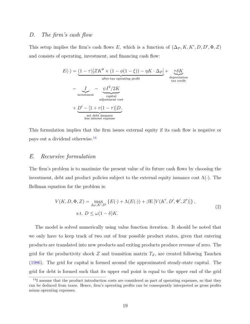
D. The firm’s cash flow

This setup implies the firm’s cash flows E, which is a function of (∆P , K,K′, D,D′,Φ, Z)

and consists of operating, investment, and financing cash flow:

E(·) = (1− τ)[ZKθ × (1− φ(1− ξ))− ηK ·∆P ]︸ ︷︷ ︸after-tax operating profit

+ τδK︸ ︷︷ ︸depreciationtax credit

− I︸︷︷︸investment

− ψI2/2K︸ ︷︷ ︸capital

adjustment cost

+D′ − [1 + r(1− τ)]D.︸ ︷︷ ︸net debt issuance

less interest expense

This formulation implies that the firm issues external equity if its cash flow is negative or

pays out a dividend otherwise.14

E. Recursive formulation

The firm’s problem is to maximize the present value of its future cash flows by choosing the

investment, debt and product policies subject to the external equity issuance cost Λ(·). The

Bellman equation for the problem is:

V (K,D,Φ, Z) = max∆P ,K′,D′

{E(·) + Λ(E(·)) + βE [V (K ′, D′,Φ′, Z ′)]} ,

s.t. D ≤ ω(1− δ)K.(2)

The model is solved numerically using value function iteration. It should be noted that

we only have to keep track of two out of four possible product states, given that entering

products are translated into new products and exiting products produce revenue of zero. The

grid for the productivity shock Z and transition matrix TZ , are created following Tauchen

(1986). The grid for capital is formed around the approximated steady-state capital. The

grid for debt is formed such that its upper end point is equal to the upper end of the grid14I assume that the product introduction costs are considered as part of operating expenses, so that they

can be deduced from taxes. Hence, firm’s operating profits can be consequently interpreted as gross profitsminus operating expenses.

19

for capital, while the lower end is half of the upper end, with a reversed sign.

F. Optimal policies

In this section, I analyze the optimal product, investment and financing policies. I derive the

first-order conditions and investigate how product portfolio decisions interact with the firm’s

choice of investment and debt. I focus on highlighting insights that are inherently different

from those stemming from standard dynamic models of the firm.

Product portfolio

As evident in the empirical evidence, the product-level dynamics implied by the endogenous

product portfolio dynamics have important implications for firm dynamics. To understand

how firms choose their product portfolios, I derive the approximate first-order condition for

product choice ∆P , assuming for simplicity that the firm does not issue equity:15

ηK︸ ︷︷ ︸product

introductioncost

≈ ZKθ(1− ξ) ∆(φ)∆(∆P )︸ ︷︷ ︸

profit increasetoday

+ βE

[∆(V (K ′, D′,Φ′(∆P ), Z ′))

∆(∆P )

]︸ ︷︷ ︸

profit increasetomorrow

. (3)

Firms will introduce new products as long as the marginal cost on the left-hand side of

Equation (3) is smaller than the marginal benefit of introducing a new product on the right-

hand side of Equation (3). The marginal cost is composed of a product introduction cost

which does not depend on the product stock. The marginal benefit depends on the discount

of old products relative to new products. Furthermore, it also changes with product portfolio

composition Φ and the profitability shock Z. For example, when the firm’s profitability

shock is more persistent (higher ρ), it has more incentives to introduce new products to reap

the benefits associated with the profitability shock whose effects last longer. Finally, the

marginal value of having an additional new product tomorrow on the firm value also enters

the marginal benefit, because the choice of today’s product portfolio affects its potential

future evolution. Thus, Equation (3) shows that investment and debt decisions of the firm

indirectly affect how it chooses its product portfolio structure.16

15In Equation 3, ∆(·) indicates the discrete derivative, defined as ∆(f(n)) = f(n+ 1)− f(n).16More specifically, Equation (3) shows that the next period stock of new products P ′

n and old products

20

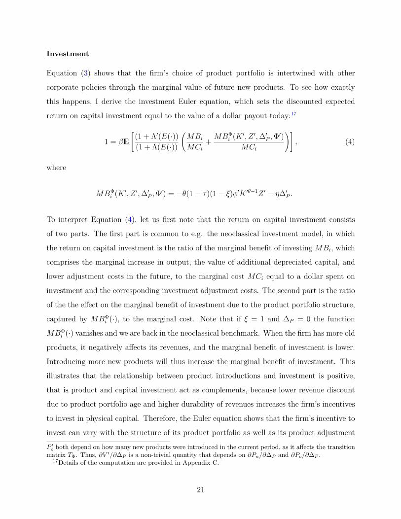
Investment

Equation (3) shows that the firm’s choice of product portfolio is intertwined with other

corporate policies through the marginal value of future new products. To see how exactly

this happens, I derive the investment Euler equation, which sets the discounted expected

return on capital investment equal to the value of a dollar payout today:17

1 = βE

[(1 + Λ′(E(·))(1 + Λ(E(·))

(MBi

MCi+ MBΦ

i (K ′, Z ′,∆′P ,Φ′)MCi

)], (4)

where

MBΦi (K ′, Z ′,∆′P ,Φ′) = −θ(1− τ)(1− ξ)φ′K ′θ−1Z ′ − η∆′P .

To interpret Equation (4), let us first note that the return on capital investment consists

of two parts. The first part is common to e.g. the neoclassical investment model, in which

the return on capital investment is the ratio of the marginal benefit of investing MBi, which

comprises the marginal increase in output, the value of additional depreciated capital, and

lower adjustment costs in the future, to the marginal cost MCi equal to a dollar spent on

investment and the corresponding investment adjustment costs. The second part is the ratio

of the the effect on the marginal benefit of investment due to the product portfolio structure,

captured by MBΦi (·), to the marginal cost. Note that if ξ = 1 and ∆P = 0 the function

MBΦi (·) vanishes and we are back in the neoclassical benchmark. When the firm has more old

products, it negatively affects its revenues, and the marginal benefit of investment is lower.

Introducing more new products will thus increase the marginal benefit of investment. This

illustrates that the relationship between product introductions and investment is positive,

that is product and capital investment act as complements, because lower revenue discount

due to product portfolio age and higher durability of revenues increases the firm’s incentives

to invest in physical capital. Therefore, the Euler equation shows that the firm’s incentive to

invest can vary with the structure of its product portfolio as well as its product adjustment

P ′o both depend on how many new products were introduced in the current period, as it affects the transition

matrix TΦ. Thus, ∂V ′/∂∆P is a non-trivial quantity that depends on ∂Pn/∂∆P and ∂Po/∂∆P .17Details of the computation are provided in Appendix C.

21

decisions. Finally, a direct computation shows that ∂MBΦi (·)/∂φ′ < 0, documenting that

the model is able to reconcile the stylized fact that product portfolio age and investment are

negatively related.

Net debt

To examine how financing and product decisions are interrelated, I combine the first-order

condition

(1 + Λ(E(·))) + βE [VD′(K ′, D′,Φ′, Z ′)] = 0 (6)

and the envelope condition associated with differentiating Eq. (2) with respect to D, which

yields

1 = βE

[(1 + Λ′(E(·)))(1 + Λ(E(·))) (1 + r(1− τ) + λ′)

], (7)

where λ is the Lagrange multiplier associated with the collateral constraint. The right-hand

side of Equation (7) is the expected discounted value of debt, which is equal to the interest

payments less the tax shield and the shadow value of relaxing the constraint on issuing

debt. The Lagrange multiplier λ indicates that debt is more valuable when the collateral

constraint is expected to bind, highlighting that the firm may have incentives to preserve

its debt capacity today to avoid reaching the collateral constraint tomorrow and having to

issue costly external equity. This result, standard in dynamic investment models such as e.g.

Gamba and Triantis (2008) or DeAngelo et al. (2011), shows that debt capacity has value

as it grants the firm more financial flexibility. One implication of this notion is the fact that

financial, investment and product policies will be intertwined: if the firm is more likely to

introduce new products tomorrow, it will follow a conservative debt policy today. Absent

positive product investment opportunities the firm will preserve its debt capacity, resulting

in a negative relationship between product portfolio age and leverage, consistent with the

stylized facts. Thus, as Equation (6) shows, even though product choice does not directly

affect the firm’s debt policy, it will have an indirect effect because it affects the firm value as

well as the probability that the firm has to incur the equity issuance cost Λ(E).18

18While the emphasis in the model is put on the fact that product dynamics affect firms’ financing decisionsonly through the ’quantitative rationing’ effects of the collateral constraint, the negative association betweenleverage is also consistent with firms issuing debt for tax reasons. Indeed, since younger product portfolios

22

III. Estimation and Identification

I structurally estimate the model to examine its quantitative implications for the relationship

between product market strategy and corporate policies. In this section, I describe the

estimation procedure, discuss the identification strategy, present the baseline results and the

cross-sectional implications.

A. Estimation

Throughout the paper, I set the tax rate τ to 20% as an approximation of the corporate

tax rate relative to personal taxes. I estimate the majority of the structural parameters

of the model using simulated method of moments (SMM). The remaining parameters are

estimated separately, but the sampling variation induced by the two-stage approach is taken

into account in the estimation procedure, which is described in detail in Appendix D. The

risk-free interest rate r is estimated at 1.4%, which is the average 3 month T-bill rate over

the sample period. I also estimate separately the probability of a ‘new’ product remaining

‘new’ pn→n and the probability of an ‘old’ product exiting po→e. These probabilities can be

inferred directly using the expected lifetime of a product implied by the model, shown in

Equation (1), and the definition of the empirical proxy. In particular, in the data a product

is considered ‘old’ if it exceeds half of its lifetime. This means that each product spends half

of its lifespan being ‘new’ and the other half being ‘old.’ In terms of the model, this implies

that

m(intr.,exit) = 12

11− pn→n

+ 12

11− qo→o

,1

1− pn→n= 1

1− qo→o.

In the data, the average lifespan of a product (weighted by revenue) is 15.94 quarters. This

implies that pn→n = 0.8746 and qo→e = 1−qo→o = 0.1254. Finally, I directly estimate the pro-

portional external equity financing cost by regressing issuance proceeds on the underwriting

fees, which implies a value of 0.0223.19

I estimate the remaining 8 parameters (θ, σ, ρ, δ, ψ, ω, η, ξ) using SMM, where θ is theincrease firms’ profits, their incentives to shield these profits from taxation are also higher and thus they willissue more debt. This channel is also present in the model.

19By doing so, I only control for direct costs of equity issuance, as in e.g. Warusawitharana and Whited(2016) or Michaels et al. (2018).

23

production function curvature, σ is the standard deviation and ρ the autocorrelation of the

profitability process; δ is the physical capital depreciation rate; ψ is the capital adjustment

cost parameter; ω is the parameter governing the collateral constraint; η is the product

introduction cost and ξ is the old-product specific revenue discount. To do so, I first solve the

model numerically, given the parameters, and generate simulated data from the model. Then,

I compute a set of moments of interest using both the simulated and actual data. The SMM

estimation procedure determines the parameter values that minimize the weighted distance

between the model-implied moments and their empirical counterparts. It is important to

note that the fact that the sample of firms in the data is fairly homogeneous speaks in favor

of using SMM, because SMM estimates the parameters of an average firm, the concept of

which is more appropriately defined in subsamples of similar firms. Appendix D provides

further details on the estimation procedure.

B. Identification

Before proceeding with estimation, I discuss the identification of the structural parameters.

SMM estimators are identified when the selected empirical moments equal the simulated

moments if and only if the structural parameters are at their true value. A sufficient condition

for this is a one-to-one mapping between a subset of structural parameters and the selected

moments, that is the moments have to vary when the structural parameters vary. Because

the firm’s investment, financing, and payout decisions are intertwined, all of the moments

are to some extent sensitive to all the parameters. However, some relationships are strongly

monotonic in the underlying parameters and as such more informative of the relationship,

thus useful for identifying the corresponding parameter. For example, the mean and variance

of operating profits are informative of µ and σ while ρ is easily identified from the serial

correlation of operating profits, which is estimated using the technique of Han and Phillips

(2010).

I select 12 moments related to firms’ operating profits, investment, net leverage and prod-

uct portfolio characteristics. I do not choose the moments arbitrarily but rather include

a wide selection of moments to understand which features of the data the model can and

cannot explain. Therefore, I examine all means, variances and serial correlations of all main

24

variables of interest that can be computed in the model. Notably, in the estimation pro-

cedure I refrain from using moments related to the size of the product portfolio (i.e. the

number of products), given that the model is unlikely to match the data on this margin, as

firms introduce products for variety of reasons that are not captured by this model (see e.g.

Hottman et al., 2016). Instead, I focus primarily on the product portfolio age and product

portfolio adjustments, which, as I argue, help identify parameters related to the product

space characteristics.

The remaining parameters are identified as follows. The physical capital depreciation rate

δ is strongly linked to the mean of investment. The capital adjustment cost parameter ψ

is identified by the variance and autocorrelation of investment, as higher adjustment costs

result in the firm smoothing its investment. The collateral constraint parameter ω is identified

by the mean of net leverage. The product introduction cost η is identified by the variance

and autocorrelation of old product share, as higher cost results in more lumpy product

introduction policy. The old-product specific discount ξ, on the other hand, is tightly linked

to the mean of old product share, as it determines the trade off the firm faces when deciding

on its product portfolio share today.

C. Estimation results

I summarize the results of the structural estimation in Table 3. Panel A contains simulated

and actual moments. Panel B reports the structural parameter estimates and their standard

errors.

Panel A suggests that the model fits the data fairly well on financial, real and product

dimensions, which is justified by the low values of t-statistics testing the difference between

the model- and data-implied moments. The only exception are the mean and serial correlation

of net leverage and the variances of investment and product portfolio age. Nevertheless, even

if the differences between simulated and actual moments are statistically significant, the

economic difference is negligible, especially for the variances and autocorrelations.

[Table 3 about here.]

Panel B documents that all model parameters are economically meaningful and statistically

25

significant. It is worth noting that the structural parameters have been estimated precisely,

as their standard errors are low, indicating that the model is well-identified.

The estimate of the product introduction cost η is equal to 0.75%, which implies that

a typical sample firm behaves as if it had to incur a cost of approximately $7.64m when

introducing a new product. While this cost appears substantial, it is required to square the

fact that firms do not continuously adjust product portfolios in the data, as the distribution

of product entry is fairly lumpy, see Figure 1. Moreover, the estimated cost is fixed and

as such can be interpreted as if it comprised both the direct costs of introduction (such as

marketing, R&D expenditures, etc.) as well as indirect ones, such as the present value of

costs related to supplying the product.

Concerning the estimate of the old-product specific discount ξ, it is equal to 0.5282,

meaning that firms act as if each old product in their portfolio only contributed 52.82% of

a new product’s revenue. The discount is thus fairly large, but consistent with the notion of

product life cycle. To gauge whether the magnitude of the estimate is sensible, I consider a

back-of-the-envelope calculation and compute the average revenue of ‘old’ and ‘new’ products

in the data. The obtained value of 59.1% suggests that the estimated value of ξ is in a

reasonable range. Barring potential measurement error, the fact that it is lower than its

data ‘counterpart’ could be explained by the fact that firms in the model do not withdraw

products by themselves, which makes the old products relatively ‘worse’ compared to the

new ones.20

The structural estimates of the remaining parameters are in range of those in extant

studies of firms’ financing and investment policy. For example, the standard deviation of the

profitability shock σ and the collateral constraint parameter ω that determines the firm’s

debt capacity are close to the ones obtained in Nikolov, Schmid, and Steri (2018) and the

persistence of the profitability process ρ is similar to the one reported in Warusawitharana

and Whited (2016) for the food manufacturing industry, which comprise the majority of the

sample firms. The only parameter that may seem on the higher end of the range compared20Moreover, products in the model do not differ with regard to their expected lifetime, whereas this is the

case in the data, the effective revenue of old but long-lasting products could be higher than that of old butshort-lasting products. I verify that this is the case by splitting the sample into two groups of firms withlong- and short-lived products and re-estimating the model. The results indicate that ξ is indeed higher inthe sample of firms with long-lived products.

26

to the existing literature is the convex investment adjustment cost ψ, estimated at 0.8786,

which results in a fairly sticky investment policy.21

D. Sample splits

The results discussed until now show that the model is able to jointly explain the corporate

investment, financing and product portfolio policies of an average sample firm. In this section,

I provide further empirical evidence of the importance of the product life cycle channel by

estimating the model on subsamples of firms that vary along key firm characteristics. In

particular, I focus on three specific sample splits. First, I investigate whether the estimated

model can reconcile differences between firms varying in the sensitivity of their products to

product life cycle. This analysis serves as a ‘sanity check’ as to whether the product life cycle

effects in the model correspond to the ones observed in the data, despite using firm-level

rather than product-level data in the estimation procedure. Second, I focus on sample splits

based on the size of product portfolio and on the degree of product market competition. This

exercise can in turn provide further insight as to how the economic forces behind product life

cycle affect corporate policies of firms differing in dimensions not explicitly captured in the

model.

Sensitivity to product life cycle

[Table 4 about here.]

I first analyze whether the model can reproduce differences across firms whose products vary

in their sensitivity to product life cycle. To this end, for each firm in the sample I estimate

a product-level regression of the form

log(rev)it = α + β × log(age)it + ηi + γc + εit,

where i and t indicate the product and the quarter, and c indicates the product’s correspond-21In a different model, Warusawitharana and Whited (2016) also obtain a much higher investment adjust-

ment cost for the food manufacturing industry.

27

ing cohort.22 I then split the firms into two groups based on the estimates of β. The firms

with the below-median (above-median) sensitivity of product-specific revenue to product age

should be less (more) exposed to product life cycle effects, for example due to the fact that

their products are more (less) durable or are less (more) susceptible to ageing.

Table 4 presents the estimation results in the two subsamples. Panel A documents that the

model-implied and data moments are relatively close, implying that the model captures well

policies of firms in both subsamples. The results also suggest that firms whose products are

less exposed to product life cycle have higher average profitability and share of old products.

The fact that these firms also adopt higher average net leverage speaks to the precautionary

savings motive of product life cycle, that should be less pronounced when firms are less

exposed to product life cycle. Firms with higher sensitivity to product life cycle invest more

on average, which is related to the fact that they tend to introduce more products and

complement it with capital investment. This is also true in the data, as the net entry rate of

these firms is approximately 3 times higher compared to the one of firms with low product life

cycle sensitivity (0.4% vs 1.2% per year, on average). The fact that this moment is not used

in the estimation procedure serves as a simple check for external validity of the subsample

analysis.

The parameter estimates in Panel B indicate that products of firms with high product

life cycle sensitivity lose about 49.79% of revenue when they become old, as compared to

38.55% for products of firms with low product life cycle sensitivity. This result shows that

the model successfully captures the intuition underlying the relationship between product

revenue and age, and as such the product-level information is not lost when aggregating data

to firm-level. The fact that average net leverage across the two subsamples is different while

the estimate of the collateral constraint parameter ω is nearly the same further reinforces

the importance of product dynamics on firms’ precautionary savings incentives. Finally, the

results imply that firms with higher product life cycle sensitivity are also more sensitive to

firm-wide productivity shocks, as the estimate of production function curvature θ is higher

for these firms, as is the standard deviation of the profitability shock. This finding suggests22Thus, I control for the cohort-specific fixed effects using the Deaton (1997) adjustment as in Argente

et al. (2019).

28

that there can be some differences in the underlying economic environment across the two

subsamples of firms, for example they may supply products in industries that may be subject

to different kinds of customer demand dynamics.

Product portfolio size

[Table 5 about here.]

I now turn to investigating the differences in estimates along dimensions not explicitly cap-

tured by the model. Table 5 shows the estimation results for firms with small and large

product portfolios, that is those with below- and above-median effective number of products,

respectively. Panel A shows that the model provides a reasonably good fit for both samples,

as the simulated and data moments are largely economically indistinguishable. The results

imply that firms with large product portfolios also tend to supply younger products, and thus

have higher operating profits. Interestingly, the size of product portfolio appears to serve

as a way for firms to diversify their revenues, as firms with large product portfolios exhibit

lower variance and higher autocorrelation of operating profits.

The corresponding parameter estimates in Panel B indicate that firms with small product

portfolios face a higher costs of introducing new products and a more pronounced old-product

specific revenue discount. These results reinforce the notion that for these firms managing

product portfolios is even more important, as they are more exposed to the product life cycle

frictions. Additionally, it is interesting to note that for firms with small product portfolios

the fraction of capital that can be collateralized ω is much lower than for firms with large

product portfolios. This result has two explanations. First, since the correlation between

product portfolio size and firms size is positive, a part of the result is simply due to small

firms having less capital (in terms of total assets) that can be pledged as collateral, consistent

with e.g. Nikolov, Schmid, and Steri (2018). However, the fact that the estimate of ω varies

substantially across the two samples suggests that the number of products also plays a critical

role, which can be consistent with firms behaving as if their intangible assets (e.g. patents

or trademarks) can be pledged as collateral as well (see e.g. Mann, 2018, Suh, 2019 or Xu,

2019).

29

Product market competition

[Table 6 about here.]

Table 6 presents the estimation results based on two subsamples differing in the degree of

product market competition.23 Investigating this dimension of the data is important for two

reasons. First, the degree of competition could affect the trade-offs determining product life

cycle, for example firms operating in more competitive markets could be forced to introduce

more new products to be able to keep up with their competitors or gain market share. Second,

the empirical literature on product markets has largely focused on this dimension of the data,

that is on how the between-firm effects affect firms’ investment and financing policy. It is

therefore instructive to examine how within-firm product market forces, such as product life

cycle, are related to corporate policies. Importantly, the measure of competition adopted in

this paper is better suited to characterize the competitive environment faced by firms as it

incorporates complete information about the product markets they operate in.

The results in Panel A suggest that firms operating in less competitive product markets

have higher operating profits, consistent with less intensive competition. Importantly, while

these firms have similar level of old product share to firms operating in competitive envi-

ronment, the effect on profitability is mitigated as these firms are less exposed to product

life cycle channel. Panel B shows that each of their old products provides about 63% of a

new product’s revenue; compared to 43% for firms subject to higher competitive pressure.

Firms in less competitive product markets also face lower costs of introducing new products.

Given that higher competition may result in products become obsolete quicker, that is ξ be-

ing lower, the results show that product life cycle is related to product market competition,

highlighting that both between- and within-firm product market forces play an important

role in shaping corporate policies. The product market competition dimension also appears

to affect the extent of product life cycle more product portfolio size does, given that the

difference in ξ across the two samples is larger than for firms differing in the size of product23This is done by first computing the HHI of each ‘market’ in which firms operate, which are defined

by product groups (see Appendix A), and then computing the firm-specific exposure to the markets, bycomputing the average HHI weighted by the firm’s share of sales in a given market. In particular, the HHIof each market is computed using all available data on private and public firms. More details about how thecompetition proxy is computed are provided in Appendix B.

30

portfolios.

IV. Analysis and Counterfactuals

In this section, I study further the implications of the estimated model. I first analyze the

numerical policy functions implied by the model and the quantitative importance of product

dynamics for variation in investment and financing policy. I then consider a number of

counterfactuals to better understand how product market strategy interacts with corporate

policies and how important its effects are for firm value.

A. Numerical policy functions

I now examine the implications of the estimated parameters for the firm’s optimal policies.

To do so, I compute the numerical policy functions {I/K,D/K,∆P} = h(K,D,Φ, Z) for

investment rate I/K, leverage D/K, and product introductions ∆P . In the discussion that

follows, I focus on two sets of policy functions. First, I fix K and D at their average values

in the simulated sample and set Z = 1 as I want to focus on the economic forces driven by

product portfolio setting. Panel A of Figure 6 plots the policy functions {I/K,D/K,∆P} =

h(Po|Φi) for a firm with a low and high number of new products, i.e. i ∈ {l, h}. Second, I

fix K, D and Φ at their average values in the simulated sample and in Panel B of Figure 6

I plot the policy functions for the profitability shocks Z: {I/K,D/K,∆P} = h(Z|Φi), again

in the two cases.

[Figure 6 about here.]

The numerical policy functions in Panel A of Figure 6 show how the firm optimally responds

to changing the product portfolio structure. In particular, the left graph in Panel A shows

that the policy function for product introductions ∆P can be characterized by an inaction

region, because the firm has to incur a fixed cost to introduce a new product. That is,

the firm only starts introducing new products once its current stock of old products (or,

alternatively, current share of old products) is sufficiently large. The threshold at which it

happens depends on the stock of new products, as firms will be less sensitive to product

portfolio structure as long as they generate sufficiently large revenue, that depends on the

31

share of old products in the portfolio.

The policy function for product introductions ∆P has natural implications for investment

and financing policy. The middle graph in Panel A illustrates that investment decreases in

the number of old products, which is consistent with the intuition behind the investment

Euler equation in Equation (4). The Euler equation also reveals the intuition behind the

spike in investment that is visible for a large number of old products, which coincides with

the firm introducing new products. That is, if the product introduction cost is sufficiently

small, the firm’s marginal benefit of investment increases in ∆P . In other words, capital and

product investment are complements: the firm wants to invest more in physical capital as

its product portfolio becomes younger to harvest the benefits of higher and more durable

operating revenue.

The right graph in Panel A documents the precautionary savings motive induced by

product dynamics, as it indicates that the firm’s leverage policy depends on its product

portfolio structure. Importantly, the firms appears to finance product introductions to a

large extent with debt, given how the increase in the policy function coincides with ∆P . It

should also be mentioned that when the share of old products in the portfolio is low, leverage

tends to decrease with Po. This happens largely because the firm has higher precautionary

savings incentives and thus values preserving debt capacity more, because it would have to

tap external financing when the old products exit and its revenue drops. Thus, given the

costly nature of external equity it is optimal for the firm to act conservatively and adopt lower

leverage. In the counterfactual experiments below, I show that this effect largely depends on

the product-level characteristics. Finally, the firm also adopts lower leverage as it benefits

less from tax shields due to lower operating income.

Panel B of Figure 6 documents how the firm optimally responds to profitability shock when

its optimal product portfolio structure is kept constant. The left graph in Panel B suggests

that the firm with a high share of old products may choose not to introduce net products

when it experiences a low realization of Z, because introducing new products is costly. The

result in the middle graph in Panel B is fairly standard in the dynamic investment models, as

investment increases with Z, but it also confirms the intuition conveyed in Panel A of Figure

6 that the firm invests less when it has an older product portfolio. That is, the product

32

dimension changes the firm’s sensitivity of investment to the profitability shock. Finally, the

right graph in Panel B illustrates that the firm’s choice of leverage varies differently with

Z, depending on its product portfolio structure. When hit by a low shock realization, the

firms tend to disinvest and use the proceeds to pay down debt, resulting in lower leverage.

Similarly, when the realization of the shock is high, the firms prefer to preserve their debt

capacity to fund future profitable investment opportunities, and thus adopt lower leverage

ratios. The only exception is the firm with a low share of old products, which also issues debt

to fund investment for a very high shock realization. It is also worth noting that for high Z

realizations, the firm with a high share of old products focuses on introducing new products,

that is renewing its product portfolio, rather than investing in capital. This coincides with

no apparent spike in leverage, unlike in Figure 6, because now the firm finances introducing

new products internally, following a high realization of Z.

B. Quantitative importance of product dynamics

I now turn to investigating the quantitative importance of product dynamics for the firm’s

corporate policies. Given that the model presents a laboratory in which, unlike in the data,

one can observe all the forces affecting investment and debt policies, we can exactly gauge

the importance of product dynamics.

[Table 7 about here.]

In Table 7, I perform a variance decomposition of the firm’s investment and leverage policy.

The results highlight that product dynamics account for as much as 20% of variation in

investment and leverage, independently of how they are measured in the model (by share of

old products or stock of new and old products separately). Moreover, most of the variation is

due to the dynamics of the stock of old products, which is intuitive given their importance in

generating the product life cycle pattern. Overall, the results suggest that product dynamics

can contribute substantially to the observed variation in corporate policies.

33

C. Counterfactuals

This subsection describes three counterfactual exercises. In the first exercise, I consider

how product-level economic forces affect firm value, firms’ precautionary savings incentives

and the relationship between product characteristics and corporate policies. In the second

exercise, I examine the impact of changing parameter values related to the product market

dimension on investment and leverage policies. I do so by varying the old-product specific

discount ξ and the probability of product exit qo→e that govern the expected benefit per

product and expected product lifetime. In the third exercise, I investigate whether allowing

for within-firm product cannibalization alters the conclusions obtained in the baseline model.

Firm value implications

I first investigate firm value effects resulting from altering product market characteristics. In

Table 8, I consider the effects of changing the cost of introducing new products η, the old

product-specific discount ξ and the individual-product transition probabilities pn→o and qo→efrom their baseline values given in Section III.

[Table 8 about here.]

The results in the second panel of Table 8 indicate that lower values of η result in higher

firm value, as product introductions become cheaper, and thus firms have more flexibility in

adjusting their product portfolio. The effects are quantitatively important as well. Increasing

η by 50% results in 5.72% lower firm value. Increasing the product introduction cost also

changes the correlations between corporate policies and product portfolio age, because the

firm’s product policy becomes more lumpy and product introductions are less frequent.

I now investigate the implications of the estimate of the old product-specific revenue

discount ξ. In the second panel of Table 8, I conduct counterfactual experiments related to

the severity of product life cycle. When setting ξ = 0, product life cycle is very severe, as

old products generate zero revenue. In contrast, ξ = 1 implies that new and old products

contribute the same amount to the firm’s cash flow. Comparing the baseline results and

those for ξ = 0 indicates that firm value is 3.55% higher due to the fact that each of their old

products generates 58% of a new product’s revenue rather than 0%. However, the firms still

34

lose from the product life cycle effects, as changing ξ from its baseline estimate of ξ = 0.5282

to ξ = 1 would increase firm value by 4.48%. All in all, this evidence suggests that introducing

products that age slower over their life cycle can bring material benefits to the firm.

It is also interesting to investigate how the correlations between corporate policies and

product portfolio age vary in these different cases from their baseline value. Not surprisingly,

making the distinction between old and new products irrelevant by setting ξ = 1 dampens

the correlations to essentially 0, as product portfolio age loses any impact. In the second

case, the relationships remain the same or become stronger. This shows that the channel

between product portfolio structure and corporate policies described in the paper is sensitive

to product characteristics.

Finally, I analyze how changing product durability affects firm value. The results in the

third panel of Table 8 show that changing the probability of a new product becoming old to

pn→o = 1 lowers firm value by 10.71%, and is much lower than increasing the probability of

an old product exiting to qo→e = 1 that results in 3.03% lower firm value. However, these can

be reconciled by the fact that the estimated old-product specific discount implies that old

products are approximately two times worse than new ones in terms of their contribution to

the firm’s revenues. Overall, the results indicate that managing product durability can also

be beneficial for firms.

Quantifying the effects on precautionary savings incentives

As argued before, the product life cycle effects induce particular precautionary savings in-

centives for firms. In the counterfactual exercise, I can examine how the magnitude of these

incentives is affected by product-level economic forces. The last column of Table 8 presents

the percentage change in firms’ debt capacity, measured as the difference between the max-

imum debt capacity ωK and net debt D (both scaled by capital K), relative to the values

implied by the estimated model.

The results suggest that product characteristics can largely magnify firms’ incentives to

preserve debt capacity. For example, changing product introduction costs affects how often

firms’ decide to introduce new products. Less frequent product introductions lower their

incentives to preserve debt capacity, because they require less funding for product introduc-

35

tions.

The effects of varying the severity of product life cycle frictions, via altering the old-

product specific discount, are even stronger and indicate that more severe product life cycle

effects result in stronger precautionary savings motives, as the firm can lose a larger fraction

of revenue due to product exit, which makes it value spare debt capacity more. This is

the reason why removing the difference between new and old products results in the firm

preserving its debt capacity less, as then the influence of the product life cycle channel is

non-existent. This finding also highlights that these precautionary savings motives induces

by product life cycle would be absent in standard dynamic models of the firm that do not

account for product-level dynamics (e.g. the AK framework).

Comparative statics: product portfolio characteristics

I now consider a different type of a counterfactual exercise by examining the effect of chang-

ing product-level characteristics on average firm policies. Figure 7 presents the resulting

comparative statics for the old product-specific revenue discount ξ in Panel A and for the

probability of old product exit qo→e in Panel B, which govern the expected benefits and the

expected longevity of each product, respectively. In each panel, I examine the effect of a

20% upward or downward change in each parameter on average investment, net leverage,

and product portfolio age. To construct these figures, I solve a model in which the values of

each parameter deviate from its baseline estimated value, and simulate using the resulting

optimal policies.

[Figure 7 about here.]

Panel A of Figure 7 documents that higher values of ξ imply that each product provides

the firm with more benefits over the same expected lifetime. As such, the firm has more

incentives to introduce new products and its product portfolio age declines, see the leftmost

graph of Panel A. This, in turn, results in the firm substituting capital for product investment,

as the latter becomes relatively cheaper for the same level of total output. As such, average

investment decreases with ξ. As for leverage, there are three main reasons why it increases

in ξ. First, the firm finances product introductions by issuing debt, especially when it has an

old product portfolio. Second, smaller old product discount ξ results in higher profits, which

36

incentivizes the firm to issue debt to benefit from tax shields. Finally, higher ξ implies that

having many old products is less risky for the firm, as they differ less from new products,

which means that the firm values preserving debt capacity less. Note that these channels are

consistent with the policy functions in Figure 6.

Panel B of Figure 7 analyzes the effects of changing the probability than an old product

exits qo→e. Essentially, this parameter determines the expected longevity of the firm’s prod-

ucts. When this probability is lower, the firm needs to introduce less new products to achieve

the same level of product portfolio longevity firm, as the existing products are expected to

survive for a longer period of time. This results in a higher average product portfolio age,

see the rightmost graph in Panel B. Thus, when the firm’s products become less durable, it

invests more in physical capital to make up for the revenue lost due to shorter lifetime of

its products. However, the effect is quantitatively smaller than in case of ξ. The firm also

adopts lower leverage to ensure that it has enough debt capacity to fund investment and

introduce new products using debt rather than resorting to costly external financing.

All in all, the results of the comparative statics further reinforce the notion that product

portfolio characteristics play a major role in shaping corporate policies.

D. The effects of cannibalization

Arguably, the product setting in the model is silent on many aspects of real-world product

portfolio management, for example the fact that introducing new products usually results in

negative externalities for firms’ existing product lines, which is known as ‘cannibalization.’

Thus, one could argue that these effects could play a major role in shaping firms’ product

market strategies. To study whether this is indeed the case, I examine how quantitatively

important the effects of cannibalization are on financing and investment.

To this end, I extend the model by explicitly allowing for a dependence between the number

of introduced products and the probability of a existing products becoming old pn→o. In the

extended model, it is parametrized as

pn→o = pn→o +∆P∑p=1

εp,

37

where ∆P is the number of products introduced by the firm and ε can be considered as a

parameter related to the firm’s elasticity of substitution between existing and new products’

revenues. Since in the model old products generate lower revenue than new ones, I effec-

tively assume that product cannibalization acts through ageing the firm’s products, which

is reasonable given that, as argued by Argente et al. (2019), product life cycle is largely due

to changes in customer preferences. In the exercise to follow, I assume that ε varies from 0

(the baseline case) to 0.0627, that is a half of pn→o. This implies that the product-specific

revenue is expected to lower by 21.9% when introducing one new product, as compared to

the “no cannibalization” benchmark.24

[Figure 8 about here.]

Figure 8 presents the effects of ε on the firm’s profitability, product portfolio age, net product

entry and net leverage. The figures indicate that controlling for potential cannibalization has

intuitive implications for corporate policies: average profitability decreases, as new product

now have shorter lifespan, which translates to higher product portfolio age, and much higher

new product entry, that nearly doubles. Finally, leverage increases for two reasons. First,

as firms finance product introductions by issuing debt, they also adopt higher leverage.

Second, higher cannibalization rate results in a more stable product portfolio structure, and

thus profitability, as both variances decrease. This lowers the firm’s precautionary savings

incentives and thus results in higher leverage.

Overall, the effect of cannibalization can magnify the effects of product life cycle, but

does not appear to alter the main mechanisms through which product dynamics interact

with corporate policies.

V. Conclusion

In this paper, I demonstrate that product market strategy has important implications for

corporate policies by developing and estimating a dynamic model of product portfolio de-24The IO and marketing literature do not specify a clear-cut candidate for the value of this parameter. For

example, Hottman et al. (2016) estimate the product elasticity of substitution due to price increases, whichimplies a cannibalization rate of 0.5 for the median firm in their sample. This means that about half of thesales of a new product introduced by a firm comes from the sales of existing products and half from the newones. That is, in this analysis I assume a less pronounced effect.

38

cisions. In line with the product life cycle channel, new products are more profitable, and

are expected to last longer than old ones, which can become obsolete. Thus, when deciding

whether the introduce new products, the firm trades off the benefits of a younger product

portfolio versus product introduction costs. I embed the product life cycle channel into a

flexible model of financing and investment that can be taken to the data by means of struc-

tural estimation. The firm’s product portfolio adjustments have direct implications for cash

flow dynamics, which connects the firm’s real, financial, and product decisions.

I document that the model provides economic rationale to the empirical relation between

product portfolio age, investment, and leverage. In particular, I find that product-level eco-

nomic forces have a significant influence on corporate investment and financing policy, as

product dynamics explain 25% of variation in investment and leverage in the model. Esti-

mates from the model imply that firms supplying fewer products, competing more intensely,

and supplying products more sensitive to ageing are also more exposed to the product life

cycle channel. The data suggests that managing the life cycle of products, by means of

introduction cost or sensitivity to ageing, yields material benefits to firms.

39

References

Abernathy, W. J. and J. M. Utterback. 1978. Patterns of industrial innovation. Technology

Review 80, 40–47.

Argente, David, Douglas Hanley, et al. 2019. Patents to Products: Innovation and Firm

Performance, Working paper, Penn State.

Argente, David, Munseob Lee, and Sara Moreira. 2018. Innovation and product reallocation

in the great recession. Journal of Monetary Economics 93, 1–20.

– . 2019. How do firms grow? The life cycle of products matters, Working paper, Penn State.

Bazdresch, Santiago, R. Jay Kahn, and Toni M. Whited. 2017. Estimating and Testing Dy-

namic Corporate Finance Models. Review of Financial Studies 31, 322–361.

Bernard, Andrew B, Stephen J Redding, and Peter K Schott. 2010. Multiple-Product Firms

and Product Switching. American Economic Review 100, 70–97.

Broda, Christian and David E. Weinstein. 2010. Product Creation and Destruction: Evidence

and Price Implications. American Economic Review 100, 691–723.

Chevalier, Judith A. 1995a. Capital Structure and Product-Market Competition: Empirical

Evidence from the Supermarket Industry. American Economic Review 85, 415–435.

– . 1995b. Do LBO Supermarkets Charge More? An Empirical Analysis of the Effects of

LBOs on Supermarket Pricing. Journal of Finance 50, 1095–1112.

Clayton, Grant. 2017. Product Market Strategy and Capital Structure: Evidence from Resale

Price Maintenance, Working paper.

D’Acunto, Francesco et al. 2018. Flexible Prices and Leverage. Journal of Financial Eco-

nomics 129, 46–68.

DeAngelo, Harry, Linda DeAngelo, and Toni M. Whited. 2011. Capital Structure Dynamics

and Transitory Debt. Journal of Financial Economics 99, 235–261.

Deaton, Angus. 1997. The analysis of household surveys. The World Bank.

Eisfeldt, Andrea and Tyler Muir. 2016. Aggregate Issuance and Savings Waves. Journal of

Monetary Economics 84, 116–133.

40

Feenstra, Robert and Hong Ma. 2007. Optimal Choice of Product Scope for Multiproduct

Firms under Monopolistic Competition. Working Paper 13703. National Bureau of Eco-

nomic Research.

Fresard, Laurent. 2010. Financial Strength and Product Market Behavior: The Real Effects

of Corporate Cash Holdings. Journal of Finance 65, 1097–1122.

Gamba, Andrea and Alexander Triantis. 2008. The value of financial flexibility. Journal of

Finance 63, 2263–2296.

Gomes, Joao. 2001. Financing Investment. American Economic Review 91, 1263–1285.

Gourio, F. and L. Rudanko. 2014. Customer Capital. Review of Economic Studies 81, 1102–

1136.

Han, Chirok and Peter Phillips. 2010. GMM Estimation for Dynamic Panels with Fixed

Effects and Strong Instruments at Unity. Econometric Theory 26, 119–151.

Hellmann, Thomas and Manju Puri. 2000. The Interaction between Product Market and

Financing Strategy: The Role of Venture Capital. Review of Financial Studies 13, 959–

984.

Hennessy, Christopher A. and Toni M. Whited. 2005. Debt Dynamics. Journal of Finance

60, 1129–1165.

– . 2007. How Costly Is External Financing? Evidence from a Structural Estimation. Journal

of Finance 62, 1705–1745.

Hoberg, Gerard and Vojislav Maksimovic. 2019. Product Life Cycles in Corporate Finance, Work-

ing paper.

Hottman, Colin J., Stephen J. Redding, and David E. Weinstein. 2016. Quantifying the

Sources of Firm Heterogeneity. Quarterly Journal of Economics 131, 1291–1364.

Kovenock, Dan and Gordon Phillips. 1995. Capital Structure and Product-Market Rivalry:

How Do We Reconcile Theory and Evidence? American Economic Review 85, 403–408.

– . 1997. Capital Structure and Product Market Behavior: An Examination of Plant Exit

and Investment Decisions. Review of Financial Studies 10, 767–803.

Lee, Bong-Soo and Beth Fisher Ingram. 1991. Simulation estimation of time-series models.

Journal of Econometrics 47, 197–205.

Levitt, Theodore. 1965. Exploit the Product Life Cycle. Harvard Business Review 35.

41

Livdan, Dmitry and Alexander Nezlobin. 2017. Investment, Tobin’s Q, and Vintage Capital:

Theory and Evidence, Working paper, Berkeley Haas.

Loderer, Claudio, Rene Stulz, and Urs Waelchli. 2017. Firm Rigidities and the Decline in

Growth Opportunities. Management Science 63, 3000–3020.

MacKay, Peter. 2003. Real Flexibility and Financial Structure: An Empirical Analysis. Review

of Financial Studies 16, 1131–1165.

Maksimovic, Vojislav. 1988. Capital Structure in Repeated Oligopolies. RAND Journal of

Economics 19, 389–407.

Mann, William. 2018. Creditor rights and innovation: Evidence from patent collateral. Jour-

nal of Financial Economics 130, 25–47.

Melser, Daniel and Iqbal A. Syed. 2015. Life Cycle Price Trends and Product Replacement:

Implications for the Measurement of Inflation. Review of Income and Wealth 62, 509–533.

Michaelides, Alexander and Serena Ng. 2000. Estimating the rational expectations model of

speculative storage: A Monte Carlo comparison of three simulation estimators. Journal of

Econometrics 96, 231–266.

Michaels, Ryan, T Beau Page, and Toni M Whited. 2018. Labor and Capital Dynamics under

Financing Frictions. Review of Finance 23, 279–323.

Newey, Whitney K. and Daniel McFadden. 1994. Chapter 36: Large sample estimation and

hypothesis testing. Handbook of Econometrics. Vol. 4. Handbook of Econometrics. Elsevier,

p. 2111–2245.

Nikolov, Boris, Lukas Schmid, and Roberto Steri. 2018. Dynamic corporate liquidity. Journal

of Financial Economics 132, 76–102.

Nikolov, Boris and Toni M. Whited. 2014. Agency Conflicts and Cash: Estimates from a

Dynamic Model. Journal of Finance 69, 1883–1921.

Parsons, Chris and Sheridan Titman. 2007. Capital structure and corporate strategy. North-

Holland Publishing Company.

Peters, Ryan H. and Lucian A. Taylor. 2017. Intangible capital and the investment-q relation.

Journal of Financial Economics 123, 251–272.

Phillips, Gordon. 1995. Increased debt and industry product markets an empirical analysis.

Journal of Financial Economics 37, 189–238.

42

Spence, Michael. 1985. Capital structure and the corporation’s product market environment.

Corporate capital structures in the United States. University of Chicago Press.

Suh, Paula. 2019. Property rights and debt financing, Working Paper, University of Georgia.

Tauchen, George. 1986. Finite State Markov Chain Approximations to Univariate and Vector

Autoregressions. Economic Letters 20, 177–181.

Titman, Sheridan. 1984. The effect of capital structure on a firm’s liquidation decision. Jour-

nal of Financial Economics 13, 137–151.

Valta, Philip. 2012. Competition and the cost of debt. Journal of Financial Economics

105, 661–682.

Warusawitharana, Missaka and Toni M. Whited. 2016. Equity Market Misvaluation, Financ-

ing, and Investment. Review of Financial Studies 29, 603–654.

Xu, Zhaoxia. 2019. Trademark collateral and debt financing, Working Paper, UNSW.

43

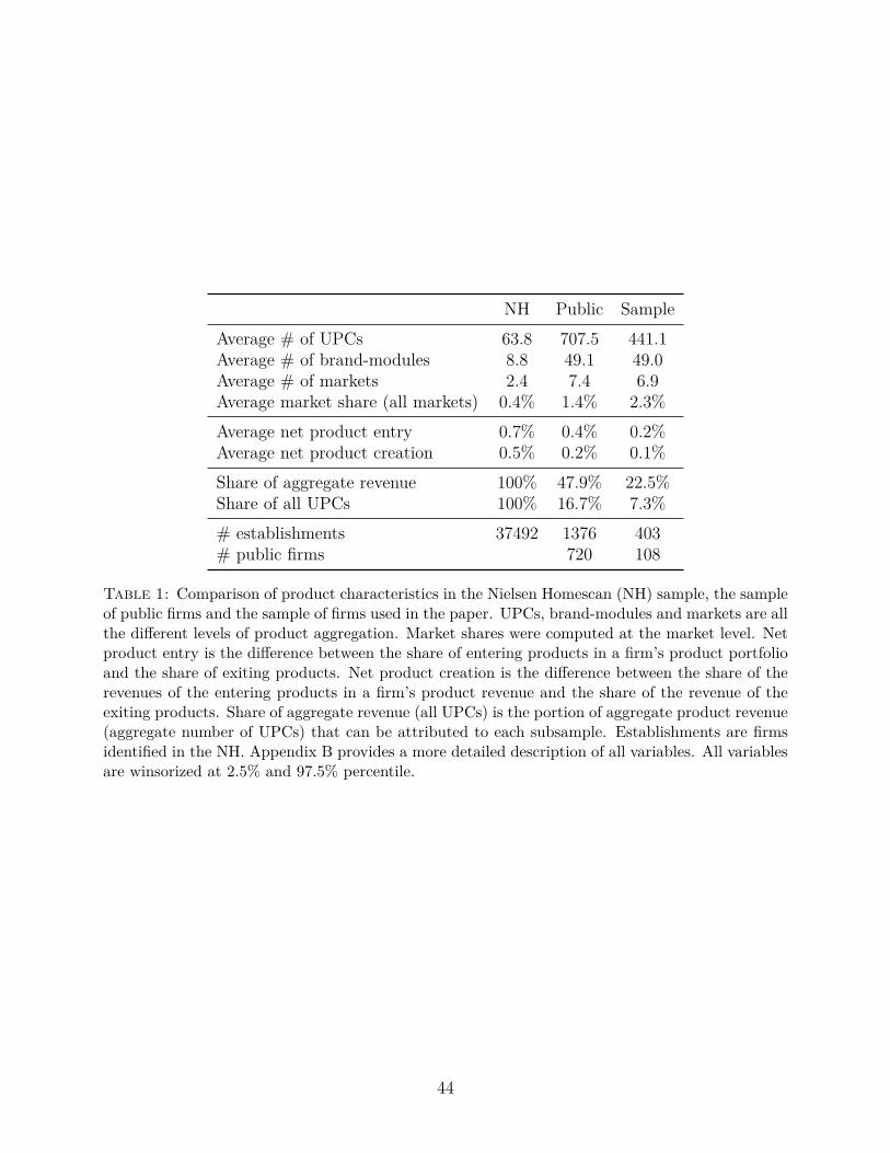
NH Public SampleAverage # of UPCs 63.8 707.5 441.1Average # of brand-modules 8.8 49.1 49.0Average # of markets 2.4 7.4 6.9Average market share (all markets) 0.4% 1.4% 2.3%Average net product entry 0.7% 0.4% 0.2%Average net product creation 0.5% 0.2% 0.1%Share of aggregate revenue 100% 47.9% 22.5%Share of all UPCs 100% 16.7% 7.3%# establishments 37492 1376 403# public firms 720 108

Table 1: Comparison of product characteristics in the Nielsen Homescan (NH) sample, the sampleof public firms and the sample of firms used in the paper. UPCs, brand-modules and markets are allthe different levels of product aggregation. Market shares were computed at the market level. Netproduct entry is the difference between the share of entering products in a firm’s product portfolioand the share of exiting products. Net product creation is the difference between the share of therevenues of the entering products in a firm’s product revenue and the share of the revenue of theexiting products. Share of aggregate revenue (all UPCs) is the portion of aggregate product revenue(aggregate number of UPCs) that can be attributed to each subsample. Establishments are firmsidentified in the NH. Appendix B provides a more detailed description of all variables. All variablesare winsorized at 2.5% and 97.5% percentile.

44

Pane

lA:s

umm

ary

stat

istic

ssiz

ead

just

men

tag

em

arke

t-to

-boo

kin

vest

men

tbo

okle

vera

geca

shfir

msiz

epr

ofita

bilit

ym

ean

58.0

660.

002

0.44

51.

882

0.02

10.

265

0.09

07.

601

0.04

0m

edia

n36

.792

0.00

00.

405

1.60

90.

017

0.27

20.

056

7.87

40.

038

std.

dev.

53.2

820.

036

0.32

41.

110

0.01

60.

169

0.09

52.

141

0.02

4N

2306

2296

2366

2366

2366

2366

2366

2366

2366

Pane

lB:p

airw

iseco

rrel

atio

nssiz

ead

just

men

tag

em

arke

t-to

-boo

kin

vest

men

tbo

okle

vera

geca

shfir

msiz

epr

ofita

bilit

ysiz

e1

adju

stm

ents

-0.0

189

1ag

e-0

.048

6-0

.047

11

mar

ket-

to-b

ook

0.08

120.

0607

0.05

681

inve

stm

ent

-0.0

965

0.04

88-0

.072

40.

215

1bo

okle

vera

ge0.

302

-0.0

282

0.06

53-0

.146

-0.0

667

1ca

sh-0

.281

0.01

140.

0127

0.40

40.

146

-0.5

061

firm

size

0.37

5-0

.021

10.

0100

-0.0

0820

-0.0

633

0.36

4-0

.210

1pr

ofita

bilit

y0.

131

0.03

58-0

.037

20.

611

0.10

7-0

.132

0.30

00.

111

1

Tab

le2:

Sum

mar

yst

atist

icso

fvar

iabl

esch

arac

teriz

ing

firm

s’pr

oduc

tpor

tfol

ioch

arac

teris

ticsa

ndco

rpor

ate

polic

ies.

Size

isth

enu

mbe

rof

prod

ucts

inpr

oduc

tpo

rtfo

lio.

Adj

ustm

ent

isth

ene

tpr

oduc

ten

try,

that

isth

edi

ffere

nce

betw

een

the

shar

eof

ente

ring

prod

ucts

ina

firm

’spr

oduc

tpor

tfol

ioan

dth

esh

are

ofex

iting

prod

ucts

.A

geis

the

shar

eof

old

prod

ucts

inpr

oduc

tpor

tfol

io,t

hati

stho

seex

ceed

ing

half

ofth

eir

lifes

pan.

Mar

ket-

to-b

ook

isth

em

arke

tva

lue

ofeq

uity

plus

book

valu

eof

debt

over

tota

lass

ets.

Inve

stm

ent

isca

pita

linv

estm

ent

over

gros

spl

ant,

prop

erty

and

equi

pmen

t.B

ook

leve

rage

isbo

okde

btov

erto

tala

sset

s.C

ash

isca

shan

dsh

ort-

term

inve

stm

ents

over

tota

lass

ets.

Firm

size

isth

elo

gof

defla

ted

tota

lass

ets.

Profi

tabi

lity

isop

erat

ing

profi

tsov

erto

tala

sset

s.A

ppen

dix

Bpr

ovid

esa

mor

ede

taile

dde

scrip

tion

ofal

lvar

iabl

es.

All

varia

bles

are

win

soriz

edat

2.5%

and

97.5

%pe

rcen

tile.

45

Panel A: MomentsSimulated Actual t-stat

Mean operating profits 0.0390 0.0401 0.5259Variance of operating profits 0.0010 0.0009 -0.3700Serial correlation of operating profits 0.2401 0.2093 -0.2749Mean investment 0.0204 0.0212 0.5619Variance of investment 0.0004 0.0006 2.1910Serial correlation of investment 0.1740 0.1742 0.0024Mean net leverage 0.2428 0.1716 -2.7116Variance of net leverage 0.0087 0.0093 0.4914Serial correlation of net leverage 0.6424 0.7848 3.0527Mean old product share 0.4301 0.4444 1.3965Variance of old product share 0.0823 0.0946 2.4429Serial correlation of old product share 0.4113 0.4392 0.3108

Panel B: ParametersParameter θ σ ρ δ ψ ω η ξ

Estimate 0.6593 0.3457 0.3392 0.0810 0.8786 0.3591 0.0075 0.5282Std. error (0.0099) (0.0272) (0.0038) (0.0055) (0.0845) (0.0222) (0.0014) (0.0124)

Table 3: Structural estimates and model-implied moments. The estimation is done using simulatedmethod of moments, which chooses model parameters by minimizing the distance between themoments from a simulated panel of firms and their data counterparts. Appendix D provides thedetails about the estimation procedure. Panel A reports the simulated and actual moments, whilePanel B the the estimated parameters and their standard errors. Standard errors are clustered atfirm-level. θ is the production function curvature; σ is the standard deviation of the profitabilityshock; ρ is the persistence of the profitability process; δ is the capital depreciation rate; ψ is theinvestment adjustment cost; ω is the parameter governing the collateral constraint; η is the productintroduction cost; ξ is the old-product specific revenue discount.

46

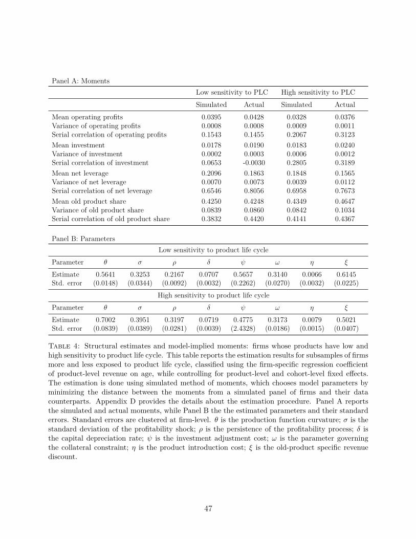
Panel A: MomentsLow sensitivity to PLC High sensitivity to PLCSimulated Actual Simulated Actual

Mean operating profits 0.0395 0.0428 0.0328 0.0376Variance of operating profits 0.0008 0.0008 0.0009 0.0011Serial correlation of operating profits 0.1543 0.1455 0.2067 0.3123Mean investment 0.0178 0.0190 0.0183 0.0240Variance of investment 0.0002 0.0003 0.0006 0.0012Serial correlation of investment 0.0653 -0.0030 0.2805 0.3189Mean net leverage 0.2096 0.1863 0.1848 0.1565Variance of net leverage 0.0070 0.0073 0.0039 0.0112Serial correlation of net leverage 0.6546 0.8056 0.6958 0.7673Mean old product share 0.4250 0.4248 0.4349 0.4647Variance of old product share 0.0839 0.0860 0.0842 0.1034Serial correlation of old product share 0.3832 0.4420 0.4141 0.4367

Panel B: ParametersLow sensitivity to product life cycle

Parameter θ σ ρ δ ψ ω η ξ

Estimate 0.5641 0.3253 0.2167 0.0707 0.5657 0.3140 0.0066 0.6145Std. error (0.0148) (0.0344) (0.0092) (0.0032) (0.2262) (0.0270) (0.0032) (0.0225)

High sensitivity to product life cycleParameter θ σ ρ δ ψ ω η ξ

Estimate 0.7002 0.3951 0.3197 0.0719 0.4775 0.3173 0.0079 0.5021Std. error (0.0839) (0.0389) (0.0281) (0.0039) (2.4328) (0.0186) (0.0015) (0.0407)

Table 4: Structural estimates and model-implied moments: firms whose products have low andhigh sensitivity to product life cycle. This table reports the estimation results for subsamples of firmsmore and less exposed to product life cycle, classified using the firm-specific regression coefficientof product-level revenue on age, while controlling for product-level and cohort-level fixed effects.The estimation is done using simulated method of moments, which chooses model parameters byminimizing the distance between the moments from a simulated panel of firms and their datacounterparts. Appendix D provides the details about the estimation procedure. Panel A reportsthe simulated and actual moments, while Panel B the the estimated parameters and their standarderrors. Standard errors are clustered at firm-level. θ is the production function curvature; σ is thestandard deviation of the profitability shock; ρ is the persistence of the profitability process; δ isthe capital depreciation rate; ψ is the investment adjustment cost; ω is the parameter governingthe collateral constraint; η is the product introduction cost; ξ is the old-product specific revenuediscount.

47

Panel A: MomentsSmall product portfolio Large product portfolioSimulated Actual Simulated Actual

Mean operating profits 0.0441 0.0391 0.0365 0.0415Variance of operating profits 0.0012 0.0014 0.0005 0.0005Serial correlation of operating profits 0.1001 0.1005 0.1970 0.4092Mean investment 0.0265 0.0239 0.0195 0.0190Variance of investment 0.0009 0.0011 0.0003 0.0003Serial correlation of investment 0.1904 0.1137 0.1738 0.1573Mean net leverage 0.1145 0.1022 0.2027 0.2396Variance of net leverage 0.0080 0.0111 0.0073 0.0062Serial correlation of net leverage 0.6137 0.7649 0.6322 0.6961Mean old product share 0.4427 0.4611 0.4292 0.4278Variance of old product share 0.0825 0.1074 0.0772 0.0736Serial correlation of old product share 0.4073 0.3897 0.3927 0.6292

Panel B: ParametersSmall product portfolio

Parameter θ σ ρ δ ψ ω η ξ

Estimate 0.7062 0.3294 0.1070 0.1041 0.5509 0.2385 0.0096 0.4334Std. error (0.0346) (0.0343) (0.0045) (0.0085) (0.4234) (0.0232) (0.0009) (0.0371)

Large product portfolioParameter θ σ ρ δ ψ ω η ξ

Estimate 0.6636 0.2610 0.2799 0.0773 0.5967 0.3043 0.0053 0.6141Std. error (0.0295) (0.0148) (0.0048) (0.0023) (0.0943) (0.0166) (0.0003) (0.0195)

Table 5: Structural estimates and model-implied moments: firms with small and large productportfolios. This table reports the estimation results for subsamples of firms with small and largeproduct portfolios, classified using the median breakpoint of the effective number of products.The estimation is done using simulated method of moments, which chooses model parameters byminimizing the distance between the moments from a simulated panel of firms and their datacounterparts. Appendix D provides the details about the estimation procedure. Panel A reportsthe simulated and actual moments, while Panel B the the estimated parameters and their standarderrors. Standard errors are clustered at firm-level. θ is the production function curvature; σ is thestandard deviation of the profitability shock; ρ is the persistence of the profitability process; δ isthe capital depreciation rate; ψ is the investment adjustment cost; ω is the parameter governingthe collateral constraint; η is the product introduction cost; ξ is the old-product specific revenuediscount.

48

Panel A: MomentsMore competitive Less competitive

Simulated Actual Simulated ActualMean operating profits 0.0335 0.0338 0.0458 0.0469Variance of operating profits 0.0008 0.0010 0.0004 0.0007Serial correlation of operating profits 0.2626 0.2141 0.2113 0.2519Mean investment 0.0208 0.0215 0.0218 0.0210Variance of investment 0.0007 0.0008 0.0004 0.0004Serial correlation of investment 0.1882 0.1501 0.1934 0.1634Mean net leverage 0.2238 0.1820 0.1825 0.1598Variance of net leverage 0.0084 0.0092 0.0059 0.0077Serial correlation of net leverage 0.5800 0.8213 0.6076 0.7242Mean old product share 0.4411 0.4322 0.4312 0.4567Variance of old product share 0.0789 0.0835 0.0763 0.0848Serial correlation of old product share 0.3882 0.3198 0.3871 0.3331

Panel B: ParametersFirms exposed to more competitive product markets

Parameter θ σ ρ δ ψ ω η ξ

Estimate 0.7457 0.3558 0.3802 0.0810 0.6455 0.3429 0.0064 0.4484Std. error (0.0324) (0.0460) (0.0041) (0.0059) (0.1860) (0.0376) (0.0019) (0.0181)

Firms exposed to less competitive product marketsParameter θ σ ρ δ ψ ω η ξ

Estimate 0.5873 0.1878 0.2813 0.0865 0.5315 0.2720 0.0063 0.6310Std. error (0.0248) (0.0295) (0.0124) (0.0050) (0.1041) (0.0130) (0.0009) (0.0093)

Table 6: Structural estimates and model-implied moments: firms exposed to more and less com-petitive product markets. This table reports the estimation results for subsamples of firms exposedto more and less competitive product markets, computed using the exposure of each firm’s salesto the HHI of each market, defined by product groups (see Appendix A). The estimation is doneusing simulated method of moments, which chooses model parameters by minimizing the distancebetween the moments from a simulated panel of firms and their data counterparts. Appendix Dprovides the details about the estimation procedure. Panel A reports the simulated and actualmoments, while Panel B the the estimated parameters and their standard errors. Standard errorsare clustered at firm-level. θ is the production function curvature; σ is the standard deviation ofthe profitability shock; ρ is the persistence of the profitability process; δ is the capital depreciationrate; ψ is the investment adjustment cost; ω is the parameter governing the collateral constraint; ηis the product introduction cost; ξ is the old-product specific revenue discount.

49

Investment Net leverageProduct portfolio age φ 0.236 0.256Stock of new products Pn 0.032 0.030Stock of old products Po 0.140 0.161

Table 7: Variance decomposition of the firm’s investment and leverage policy. I compute the TypeIII partial sum of squares for each variable in the model and then normalize each estimate by thetotal variance. That is, each number represents the % of total variance explained by the variable.

50

%∆

firm

Cor

r(·,

age)

%∆

debt

valu

em

tbin

vle

vca

paci

tyBa

selin

e0.

00%

-0.2

08-0

.088

-0.0

600.

00%

50%

lowe

rpr

oduc

tin

trod

uctio

nco

stη

9.14

%-0

.113

-0.0

900.

000

11.3

8%50

%hi

gher

prod

uct

intr

oduc

tion

costη

-5.7

2%-0

.231

0.00

4-0

.171

-43.

59%

Old

prod

uct

gene

rate

sno

reve

nueξ

=0

-3.5

5%-0

.045

-0.0

44-0

.201

117.

54%

Old

and

new

prod

ucts

are

the

sam

eξ

=1

4.48

%0.

000

0.00

0-0

.009

-61.

41%

New

prod

uct

imm

edia

tely

beco

mes

oldp n→o

=1

-10.

71%

-0.2

030.

081

0.09

0-5

9.40

%O

ldpr

oduc

tim

med

iate

lyex

itsq o→e

=1

-3.0

3%0.

009

-0.0

19-0

.154

-62.

73%

Tab

le8:

The

tabl

ere

port

sou

tcom

esco

rres

pond

ing

toal

tern

ativ

em

odel

para

met

rizat

ions

byva

ryin

gth

epr

oduc

tin

trod

uctio

nco

stη

(firs

tpan

el),

the

old-

prod

ucts

peci

ficre

venu

edi

scou

ntξ

(sec

ond

pane

l),an

dth

ein

divi

dual

-pro

duct

tran

sitio

npr

obab

ilitie

span

dq

(thi

rdpa

nel).

The

first

colu

mn

repo

rts

the

%ch

ange

inth

eav

erag

em

arke

t-to

-boo

kre

lativ

eto

base

line

estim

atio

nre

sults

,the

thre

efo

llow

ing

colu

mns

the

corr

elat

ion

betw

een

prod

uct

port

folio

age

and

mar

ket-

to-b

ook,

inve

stm

ent,

and

leve

rage

,res

pect

ivel

y,an

dth

ela

stco

lum

nth

e%

chan

gein

the

aver

age

debt

capa

city

(mea

sure

das

the

diffe

renc

ebe

twee

nm

axim

umde

btca

paci

tyωK

and

curr

ent

net

debt

,bot

has

afr

actio

nof

capi

tal)

rela

tive

toba

selin

ees

timat

ion

resu

lts.

51

Product portfolio size Product portfolio adjustments Product portfolio ageH

istog

ram

0.0

5.1

.15

.2

0 50 100 150 200 250

0.1

.2.3

.4.5

−.2 −.1 0 .1 .2

0.0

5.1

.15

0 .2 .4 .6 .8 1

Mar

ket-

to-b

ook

1.4

1.5

51.7

1.8

52

2.1

5

1 2 3 4 1.4

1.5

51.7

1.8

52

2.1

5

1 2 3 4 1.4

1.5

51.7

1.8

52

2.1

5

1 2 3 4

Inve

stm

ent

.01

.015

.02

.025

1 2 3 4 .01

.015

.02

.025

1 2 3 4 .01

.015

.02

.025

1 2 3 4

Book

leve

rage

.15

.2.2

5.3

.35

1 2 3 4 .15

.2.2

5.3

.35

1 2 3 4 .15

.2.2

5.3

.35

1 2 3 4

Cas

h0

.03

.06

.09

.12

.15

1 2 3 4

0.0

3.0

6.0

9.1

2.1

5

1 2 3 4

0.0

3.0

6.0

9.1

2.1

5

1 2 3 4

Figure 1: The graphs summarize the firms’ product portfolio structure and illustrate the relationshipsbetween firms’ corporate policies and product characteristics. The first row contains the histograms ofproduct portfolio size, adjustments, and age. Rows two to 5 contain the relationship between each productportfolio- and firm characteristic. In each of these graphs, every product portfolio characteristic is divided infour equally-sized bins and the corresponding average firm characteristic in every bin is computed. AppendixB provides a description of all variables. 52

0 0.2 0.4 0.6 0.8 10.038

0.039

0.040

0.041Profitability

0 0.2 0.4 0.6 0.8 10.000

0.005

0.010

0.015

0.020Product sales growth

0 0.2 0.4 0.6 0.8 1

0.010

0.011

0.012

0.013Cash flow volatility

0 0.2 0.4 0.6 0.8 1

0.060

0.065

0.070

0.075Cost of sales

Figure 2: The figure shows how profitability, product revenue growth, cash flow volatility, andcost of sales change with product portfolio age. The solid lines are obtained from local polynomialregressions of each variable on the product portfolio age proxy using an Epanechnikov kernel functionwith a rule-of-thumb bandwidth estimator and local-mean smoothing. Appendix B provides adescription of all variables.

53

0 0.2 0.4 0.6 0.8 1-0.050

-0.025

0.000

0.025

0.050Residual market-to-book

0 0.2 0.4 0.6 0.8 1-0.002

-0.001

0.000

0.001Residual investment

0 0.2 0.4 0.6 0.8 1-0.002

-0.001

0.000

0.001

0.002

Residual net book leverage

Figure 3: The figure shows the relationship between product portfolio age and firms’ unexplainedmarket-to-book, investment and leverage. The solid lines are obtained from local polynomial re-gressions of each variable on the product portfolio age proxy using an Epanechnikov kernel functionwith a rule-of-thumb bandwidth estimator and local-mean smoothing. The controls used to com-pute the predicted values include profitability, investment, leverage, size, cash flow volatility formarket-to-book, profitability, size, cash flow volatility, market-to-book and tangibility for leverage,and size, cash flow, and market-to-book for investment. All models control for firm and time fixedeffects. Appendix B provides a description of all variables.

54

Panel A: Investment residuals

4 6 8 10

-0.001

-0.0005

0

0.0005

Firm size1 2 3 4

-0.001

0

0.001

0.002

Market-to-book

Panel B: Leverage residuals

-0.02 0 0.02 0.04 0.06 0.08 0.10-0.01

-0.005

0

0.005

0.01

Profitability0.1 0.3 0.5 0.7 0.9

-0.002

0

0.002

0.004

0.006

Tangibility

Figure 4: Assessing the significance of product portfolio age for corporate policies. All graphsare obtained from local polynomial regressions of the residuals from an investment (or leverage)regression on a given variable, using an Epanechnikov kernel function with a rule-of-thumb band-width estimator and local-mean smoothing. The controls used to compute the investment residualsinclude size, cash flow, and market-to-book. The controls used to compute the leverage residualsinclude profitability, size, cash flow volatility, market-to-book, share of old products, and tangibilityfor profitability and profitability, size, cash flow volatility, market-to-book, and share of old productsfor tangibility. All regression models control for firm and time fixed effects. Appendix B providesa description of all variables.

55

time

revenue

0

x

tintr. = tn

‘new’, p ∈ Pn

to

ξ · x

‘old’, p ∈ Po

te ∞

‘exit’

Figure 5: Graphical representation of each product’s evolution in the model.

56

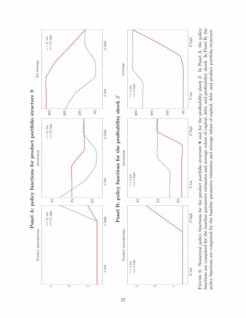
Pan

elA

:po

licy

func

tion

sfo

rpr

oduc

tpo

rtfo

liost

ruct

ure

Φ

φlo

wφ

high

135

Prod

uct

intr

oduc

tions

Pn

low

Pn

high

φlo

wφ

high

0%2%4%

Inve

stm

ent

Pn

low

Pn

high

φlo

wφ

high

0%10%

20%

30%

Net

leve

rage

Pn

low

Pn

high

Pan

elB

:po

licy

func

tion

sfo

rth

epr

ofita

bilit

ysh

ockZ

Zlo

wZ

high

135

Prod

uct

intr

oduc

tions

φlo

wφ

high

Zlo

wZ

high

0%2%4%

Inve

stm

ent

φlo

wφ

high

Zlo

wZ

high

0%10%

20%

30%

Leve

rage

φlo

wφ

high

Fig

ure

6:N

umer

ical

polic

yfu

nctio

nsfo

rth

epr

oduc

tpo

rtfo

liost

ruct

ure

Φan

dfo

rth

epr

ofita

bilit

ysh

ockZ

.In

Pane

lA,t

hepo

licy

func

tions

are

com

pute

dfo

rth

eba

selin

epa

ram

eter

estim

ates

and

aver

age

valu

esof

capi

tal,

debt

,and

profi

tabi

lity

shoc

k.In

Pane

lB,t

hepo

licy

func

tions

are

com

pute

dfo

rth

eba

selin

epa

ram

eter

estim

ates

and

aver

age

valu

esof

capi

tal,

debt

,and

prod

uct

port

folio

stru

ctur

e.

57

Pan

elA

:ol

dpr

oduc

t-sp

ecifi

cre

venu

edi

scou

ntξ

−20

%−15

%−10

%−

5%0%

5%10

%15

%20

%

41.5

%

42%

42.5

%

43%

43.5

%

44%

44.5

%Pr

oduc

tpo

rtfo

lioag

e

−20

%−15

%−10

%−

5%0%

5%10

%15

%20

%8.

13%

8.16

%

8.19

%

8.22

%

8.25

%

Inve

stm

ent

−20

%−15

%−10

%−

5%0%

5%10

%15

%20

%

23%

24%

25%

26%

27%

28%

Net

leve

rage

Pan

elB

:pr

obab

ility

ofol

dpr

oduc

tex

itq o→e

−20

%−15

%−10

%−

5%0%

5%10

%15

%20

%38

%

39%

40%

41%

42%

43%

44%

45%

Prod

uct

port

folio

age

−20

%−15

%−10

%−

5%0%

5%10

%15

%20

%8.

15%

8.16

%

8.17

%

8.18

%

8.19

%

Inve

stm

ent

−20

%−15

%−10

%−

5%0%

5%10

%15

%20

%

23%

24%

25%

26%

27%

28%

29%

30%

Net

leve

rage

Fig

ure

7:C

ompa

rativ

est

atic

sof

prod

uct-

rela

ted

para

met

ers.

Each

poin

ton

the

curv

eco

rres

pond

sto

mom

ents

from

aco

unte

rfac

tual

expe

rimen

t,st

artin

gfr

omth

eba

selin

ees

timat

esof

stru

ctur

alpa

ram

eter

san

dch

angi

ngon

lyth

ere

spec

tive

para

met

erby

20%

upan

d20

%do

wn.

Each

curv

eis

apo

lyno

mia

lint

erpo

latio

nof

mom

ents

from

adi

scre

tese

tof

coun

terf

actu

alex

perim

ents

.

58

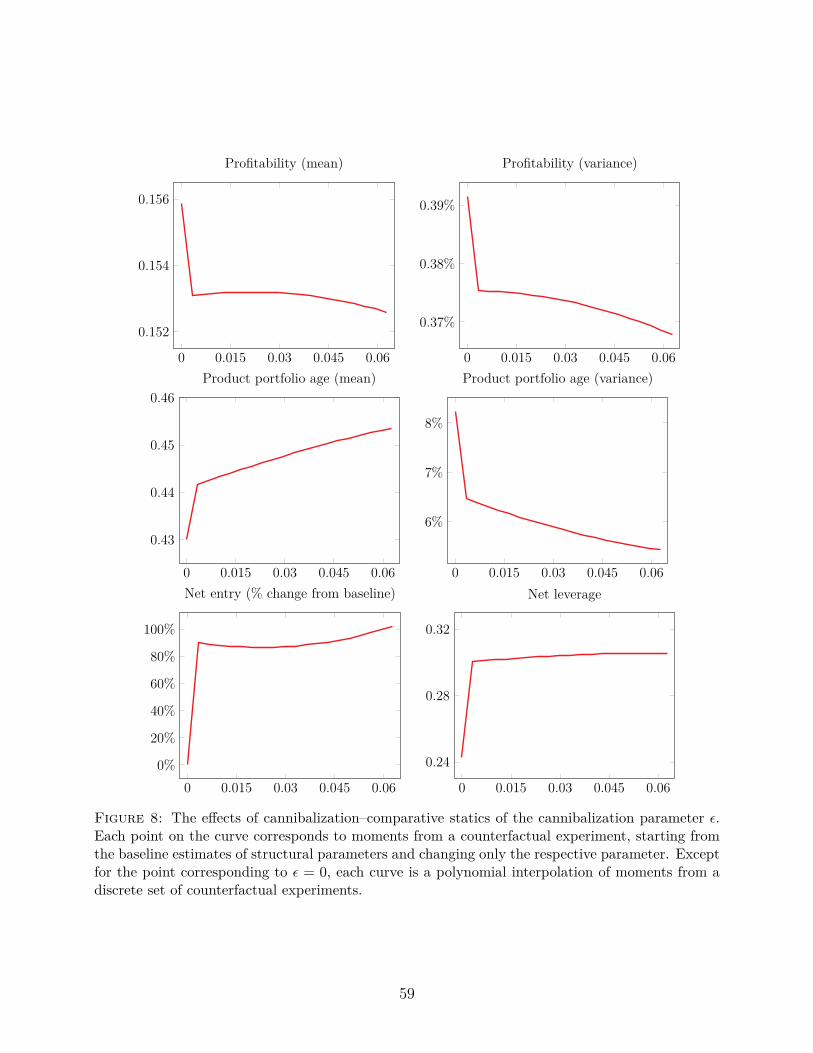
0 0.015 0.03 0.045 0.06

0.152

0.154

0.156

Profitability (mean)

0 0.015 0.03 0.045 0.06

0.37%

0.38%

0.39%

Profitability (variance)

0 0.015 0.03 0.045 0.06

0.43

0.44

0.45

0.46Product portfolio age (mean)

0 0.015 0.03 0.045 0.06

6%

7%

8%

Product portfolio age (variance)

0 0.015 0.03 0.045 0.060%

20%

40%

60%

80%

100%

Net entry (% change from baseline)

0 0.015 0.03 0.045 0.06

0.24

0.28

0.32

Net leverage

Figure 8: The effects of cannibalization–comparative statics of the cannibalization parameter ε.Each point on the curve corresponds to moments from a counterfactual experiment, starting fromthe baseline estimates of structural parameters and changing only the respective parameter. Exceptfor the point corresponding to ε = 0, each curve is a polynomial interpolation of moments from adiscrete set of counterfactual experiments.

59

Appendix

A. Product market data

A. Data description

I use the AC Nielsen Homescan (NH) data to obtain information about firms’ product market

strategies. An extensive description of the database can also be found in e.g. Broda and

Weinstein (2010) or Hottman, Redding, and Weinstein (2016). The data contains three

dimensions: household, product and time. Each household in the sample reports the prices

and quantities of items purchased during each shopping trip and any potential discounts or

deals associated with the purchases. Overall, the data contains a representative sample of

approximately 40,000-60,000 households stratified into 61 geographic areas in the US. The

sample is designed so that it can be projected to the total US population (projection factors

are available). In total, the data spans over the period of 14 years (2004–2017).25

A.1 Product classification in NH

Each product in the data belongs to specific categories, varying in their granularity. There

are categories such as Departments (10), Product Groups (≈125), Modules (≈1,075) and

UPC codes (≈4.3 million out of which ≈2.3 million are present in the consumer panel files).

Most products also have a specific brand. An example of product classification can be found

in Table A.1.

Table A.1: Details of ‘NESTLE USA 8.47 OZ (240g) Nescafe Frothe Latte Coffee Drink’

Compustatidentifier

GS1identifier

productidentifier

productdepartment

productgroup product module product

brand

(6 digits) (13 digits) (12 digits) DRYGROCERY CANDY CANDY –

CHOCOLATE HERSHEY’S KISSES

The most granular level of product categories is the UPC code. Each UPC code is 12-

digit long and the first 6 to 11 digits are a unique identifier of the firm to which the product25It should be noted that Nielsen Homescan database by construction focuses on nondurable consumer

goods, so most apparel, electronics and home furnishing purchases may not be recorded.

60

belongs (‘GCP code’). However, firms can have many GCP codes. To obtain all possible

combinations, all GCP codes are collected using the GLN code, issued by GS1 (which also

manages the issuance of the UPC codes). The GLN code is used to identify physical locations

or legal entities of the firms. The key is 12 digits long and comprises a GS1 Company Prefix,

Location Reference, and Check Digit. Both the GCP code as well as the GLN codes are

obtained from the GEPIR database provided by POD, which additionally contains the full

name and the address of each firm. Overall, the POD database is able to match 3.4 millions

UPCs (≈ 78% of all available products and ≈ 96% of product data available in the consumer

panel files) which belong to 51,592 firms (37,492 firms in the panel data).

Table A.2 contains the summary statistics of firm-level number of products per category.

It indicates the large degree of heterogeneity in the data: while an average firm owns roughly

8.82 products, a typical (median) firm owns only 2. Similar conclusions can be drawn from

looking at other classifications of products.

mean sd q1 med q3 min max

# UPCs 63.8 493.43 2 5 17 1 36352# brand-modules 8.82 37.28 1 2 5 1 1738# brands 4.67 17.69 1 1 3 1 1126# product modules 4.83 22.62 1 2 3 1 795# product groups 2.44 5.12 1 1 2 1 111# departments 1.37 0.89 1 1 1 1 11

Table A.2: Summary statistics of different product classifications of 37,492 firms.

A.2 Merging with Compustat

The matched firm-product data can be merged with accounting data from Compustat by

using text matching of firm names. However, many public firms own multiple subsidiaries

and the firm-product data could thus contain their name rather the one of the ultimate

parent. For example, in the data P&G directly ‘owns’ most if not all of the products while

Newell Brands only owns its products through some of the 121 subsidiaries. As such, I obtain

the names of subsidiaries of each firm in Compustat from Capital IQ.

The text matching procedure is conducted using fuzzy merging based on several ‘similar-

61

ity’ functions and the matches were manually verified. The matching scores are based on

GEDSCORE, SPEDIS and % of the same 3-character combinations of one company name

in the other. All punctuation, special characters and common words are removed before

conducting the comparison. After the merge, I manually add firms with at least 200 UPC

codes to the data (out of all unmatched firms with more than 800 UPC codes – 477 firms –

15% turned out to be public or subsidiaries of public firms). In total, I was able to merge

1376 GLN-level firms (or subsidiaries) from the firm-product data, which correspond to 720

US-headquartered Compustat firms.

To verify that the matching procedure is reasonable, I analyze the ‘sales share’, i.e. the

ratio of the projected sales (to the whole US; computed using the projection factors in the

data) of each matched Compustat firm-quarter to its actual sales in that quarter, which are

available in the data. I only focus on 2-digit SIC industries with at least two matched firms.

Table A.3 contains the summary statistics on sales share for the whole sample as well as for

2-digit SIC industries.

mean sd p25 median p75 N

Agricultural Production - Crops 0.530 0.221 0.316 0.529 0.723 110Food & Kindred Products 0.580 0.469 0.221 0.487 0.797 2573Tobacco Products 0.181 0.093 0.099 0.141 0.264 118Chemical & Allied Products 0.503 0.564 0.103 0.263 0.861 616Rubber & Miscellaneous Plastics Products 0.608 0.632 0.076 0.419 1.106 123Electronic & Other Electric Equipment 0.369 0.339 0.098 0.264 0.469 206Total 0.542 0.481 0.173 0.404 0.784 3746

Table A.3: Sales’ shares of matched firms. All variables are winsorized at 2.5% and 97.5%percentile.

Table A.3 suggests that not all industries are equally well-represented in the data. For

example, Agriculture and Food industries are relatively well matched. Other industries, such

as Electronic and Chemicals, are characterized by large degree of within-industry dispersion

in sales share. This is partially related to the fact that AC Nielsen data focuses on particular

product categories, which are only partially present in some industries (e.g. one could think

about Procter and Gamble, whose product portfolio is relatively well-captured in the data,

but which is primarily in the Chemicals sector also containing other firms with low sales

62

share). However, the matched sample contains primarily firms from the ‘food’ industry, which

comprises two SIC2 codes: 01 and 20, and these firms rely heavily on the retail channel in

generating sales.

B. Sample selection

To refine the data for further empirical analysis, I first apply the standard Compustat data

filters: I remove firms with missing data on any variables used in structural estimation,

market-to-book larger than 15 or negative book equity. Based on the matched sample, I

remove all financial conglomerates (SIC≥ 6000). I require that firm’s projected sales share

(that is, the ratio of Homescan-based sales to accounting measures of sales reported in Com-

pustat) be at least 5% and no more than 150% of its total sales on average. Moreover, I

only keep firms in industries in which the average projected sales share is at least 10%. I

also remove all firms which have on average less than 20 UPC codes. Even though I control

for the sales share in the empirical analysis, this filter is important as it disposes of firms

that do no rely on retail channel (so the main mechanism is unlikely to matter) or that were

plausibly mismatched. As an example, this filter removes firms such as American Crystal

Sugar Co or Archer-Daniels-Midland Co. for whom the retail channel is clearly of secondary

if not tertiary importance. I winsorize the remaining data at 2.5% and 97.5% level. The final

sample spans 2004Q1 to 2017Q4 and contains 2,366 firm-quarter observations.

B. Data and stylized facts

A. Definitions of variables

This section presents the definitions of variables used throughout the paper.

1. Product portfolio size – effective number of products at level x, x ∈ [upc, bm]:

eff no prodit = 1/rc xit,

63

where rx x is the revenue concentration at level x:

rc xit = Hit − 1/Nit

1− 1/Nit

, with Hit =Nit∑x=1

(r salext∑Nitx=1 r salext

)2

,

where r salext are the estimated aggregate retail sales for each x ∈ {upc, bm} product

at time t. To see where the measure for the effective number of products stems from,

suppose that a firm supplies N products. Then its revenue concentration is rc =∑Ni=1 s

2i , where si is the share of product i in the firm’s sales. Assuming all products

provide equal revenue, their revenue share is si = s = 1/N , thus the HHI is now

rc = ∑Ni=1 1/N2 = N/N2 = 1/N , which implies that we can back out the ‘effective’

number of products as eff no prod = 1/rc.

2. Product portfolio adjustments – net product entry:

neit = (# product introductions(it)−# product withdrawals(it))/total # products(it),

where an ‘introduction’ indicates a new product that has never been offered by firm i

before time t and a ‘withdrawal’ indicates that a product was no longer supplied by

firm i after time t. I also consider net product creation:

ncit = (revenue of entering products(it)−revenue of exiting products(it))/total revenue(it),

where an ‘entry’ indicates an introductions of a new product that has never been offered

by firm i before time t and an ‘exit’ indicates a product that was no longer supplied by

firm i after time t.

3. Product portfolio age – weighted share of old products in the portfolio:

age(x) = weighted # of products with age exceeding x% of lifespantotal # of products ,

where the weights correspond to product-specific revenues.

4. Market-to-book: book value of debt plus market value of equity over total assets.

5. Investment: capital expenditure minus asset sales over gross plant, property and

64

equipment.

6. Net book leverage: book debt minus cash and short-term investments over book

debt plus book equity.

7. Cash: cash and short-term investments over total assets.

8. Firm size: natural logarithm of real total assets.

9. Profitability: operating income over total assets.

10. Cost of sales: general and administrative expense over total assets.

11. Implied competition:

ihhiit =M∑m=1

smitHHImt,

where sm,i,t is the share of firm’s i sales in market m at time t, and HHIm,t is the

Herfindahl of market m at time t, computed using all firms available in the sample,

both public and private.

12. Cash flow volatility: the rolling standard deviations of profitability, computed over the

past 8 quarters.

C. Model solution

A. Product transition matrix

To get the product transition matrix TΦ, I have to consider all possible states of the products

in the future Φ′ = (P ′n, P ′o) conditional on Φ = (Pn, Po). We know that Pe = (P ′n + P ′o) −

(Pn + Po) products exit. There are 32 cases in total to consider. Two examples of how these

are computed are as follows, note that for the purpose of computing the transition matrix

I also allow old products to transition to being new (which in the main specification is not

allowed) hence I need to know both qo→o and qo→e:

• P ′n = Pn and P ′o = Po:

Pr(Φ′|Φ) =min(Po,Pn)∑

k=0Bin(max(Pn − k, 0), Pn, pn→n)× Trin(k, Pe, Po, qo→o, qo→e).

65

04

812

1620

-0.0

010

0.00

1

0.00

2

Aver

age

prod

uct

age

(w)

0.5

11.

52

2.5

3

-0.0

02

-0.0

010

0.00

1

Aver

age

log(

age)

,(w

)

00.

20.

40.

60.

81

-0.0

010

0.00

1

Shar

eof

old

prod

ucts

(0.5

;uw

)

00.

20.

40.

60.

81

-0.0

02

-0.0

010

0.00

1

Shar

eof

old

prod

ucts

(w;0

.75)

00.

20.

40.

60.

81

-0.0

02

-0.0

010

0.00

1

Shar

eof

old

prod

ucts

(w;0

.9)

00.

20.

40.

60.

81

-0.0

02

-0.0

010

0.00

1

Shar

eof

old

prod

ucts

(w;0

.75;

bm)

Fig

ure

B.1

:R

obus

tnes

sch

eck:

defin

ing

prod

uct

port

folio

age.

Each

grap

his

obta

ined

from

loca

lpol

ynom

ialr

egre

ssio

nof

the

resid

uals

from

anin

vest

men

tre

gres

sion

ona

give

npr

oduc

tpo

rtfo

lioag

eva

riabl

e,us

ing

anEp

anec

hnik

ovke

rnel

func

tion

with

aru

le-o

f-thu

mb

band

wid

thes

timat

oran

dlo

cal-m

ean

smoo

thin

g.T

heco

ntro

lsus

edto

com

pute

the

inve

stm

ent

resid

uals

incl

ude

size,

cash

flow

,an

dm

arke

t-to

-boo

k.w

indi

cate

sth

atpr

oduc

t-le

velr

even

uew

eigh

tsw

ere

used

(uw

-not

used

).0.

5,0.

75,0.9

are

the

tres

hold

sus

edto

defin

ean

old

prod

uct,

i.e.

one

that

exce

eds

50%

,75

%an

d90

%of

itslif

espa

n,re

spec

tivel

y.bm

indi

cate

sth

atbr

and-

mod

ule

leve

lwas

used

rath

erth

anU

PC-le

vel.

App

endi

xB

prov

ides

ade

scrip

tion

ofal

lvar

iabl

es.

66

• P ′n = Pn and P ′o < Po:

Pr(Φ′|Φ) =min(P ′

n,Po−Pe)∑k=0

Bin(max(Pn − k, 0), Pn, pn→n)× Trin(k, Pe, Po, qo→o, qo→e).

Given that solving the model on the grid means that that the firm can have at most Pn new

products and Po old products, the transition matrix will be ill-defined in certain states, as

the probabilities will not sum to one. To alleviate this issue, I normalize each such state by

distributing the residual probability across all states with non-zero probability, with weights

proportional to ex ante transition probabilities to these states. The results are robust to

considering alternative normalization schemes, e.g. attributing the residual probability to

current state.

B. Further details on computing the investment Euler equation

To compute the investment Euler equation, I first take the first-oder condition of (2) with

respect to K ′, which yields

(1 + Λ(E(·)))(−1−ΨK′(K,K ′)) + βE [VK′(K ′, D′,Φ′, Z ′)] = 0

as well as the envelope condition that gives

VK(K,D,Φ, Z) = (1+Λ(E(·)))(1−τ)[(1−φ(1−ξ))θKθ−1Z−η∆P ]+τδ+(1−δ)−ΨK(K,K ′).

Combining them both yields the investment Euler equation

1 = βE

[FΛ

11 + ψ

2 i

((1− τ)θK ′θ−1Z ′ + 1− (1− τ)δ + ψi′

(12i′ + 1− δ

)

− (1− τ)(φ′(1− ξ)θK ′θ−1Z ′ + η∆′P

))],

where

FΛ = (1 + Λ′(E(·)))(1 + Λ(E(·)))

67

is the ‘external financing discount factor,’ see e.g. Eisfeldt and Muir (2016). Thus, the

marginal benefit (MBi) to investment in physical capital and the marginal cost (MCi) are

MBi = (1− τ)θK ′θ−1Z ′ + 1− (1− τ)δ + ψi′(1

2i′ + 1− δ

),

MCi = 1 + ψi,

MBΦi (·) = −(1− τ)

(φ′(1− ξ)θK ′θ−1Z ′ + η∆′P

),

where i = I/K. Thus, we derived Equation (4):

1 = βE

[(1 + Λ′(E(·))(1 + Λ(E(·))

(MBi

MCi+ MBΦ

i (K ′, Z ′,∆′P ,Φ′)MCi

)].

Verifying that ∂MBΦi (·)/∂φ′ < 0 follows from a direct computation:

∂MBΦi (·)

∂φ′= −(1− τ)(1− ξ)θK ′θ−1Z ′ < 0.

D. Structural estimation

I follow Lee and Ingram (1991) when estimating the model using structural method of mo-

ments. As in Hennessy and Whited (2007), I extract as much of observed heterogeneity

from data as possible to make the model- and data-implied moments comparable, that is I

use within-transformed variables to compute all moments except for means, which are com-

puted using the raw data. Let the pooled time series of all firms be xi = x1, . . . , xN , where

N = n × T is the total number of firm-year observations. Using the transformed data, I

compute a set of moments h(xi).

I create the simulated moments by first solving solving the model given a vector of pa-

rameters β = (θ, σ, ρ, ψ, η, ω, ξ) and then generating simulated data y from the model. I

simulate S = 10 datasets of N = 2, 000 firm-quarters, following Michaelides and Ng (2000),

who find that a simulation estimator behaves well in finite samples if the simulated sample

is approximately ten times as large as the actual data sample. The resulting moments in a

given simulated sample are given by the vector h(ys, β).

68

The simulated methods of moments estimator β is then the solution to

β = arg minβ

[g(x)− g(y, β)]′W [g(x)− g(y, β)] ,

where g(x) = 1N

∑Ni=1 h(xi) and g(y, β) = 1

S

∑Ss=1 h(ys, β) are the sample means of the actual

and model-implied data, and W a positive definite weight matrix. I use the optimal clustered

weight matrix constructed as in Bazdresch et al. (2017). I use simulated annealing to find

the optimum to the minimization problem.

Under mild regularity conditions, the SMM estimator is asymptotically normal

√N(β − β) d−→ N (0, V ) ,

where V is the covariance matrix adjusted for sampling variation induced by estimating a

number of parameters outside of the model, see Newey and McFadden (1994).

69