Procuring Commodities: Request for Quote or Reverse Auctions?1

Jason Shachat Wang Yanan Institute for Studies in Economics -WISE

Xiamen University jason.shachat@gmail.com

Current version: February 8, 2009

Abstract: We examine the relative performances of reverse auctions and request for quotes in a simple commodity environment. Enterprises embarking on a reverse auction initiative often start with their commodity purchases. We conduct laboratory experiments and find that this is a poor starting point. Both the mean and variance of prices when sourcing through reverse auctions. With respect to the general investigation of auctions, the request for quote is the mirror image of a first price sealed bid auction and has the same symmetric Nash equilibrium. However, the request for quote allows identification of simple behavioral rules such as always bidding a percentage of your signal, which is indistinct from Nash equilibrium strategies in the sell auction counterpart. Consequently we estimate that one-fourth of the subjects follow a simple mark-up rule and approximately two-thirds follow a strategic Nash equilibrium strategy.

1 We thank the National University of Singapore for financial support, and also the NUS School Business and New York University for the use of their facilities.

1

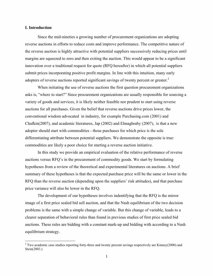
I. Introduction

Since the mid-nineties a growing number of procurement organizations are adopting

reverse auctions in efforts to reduce costs and improve performance. The competitive nature of

the reverse auction is highly attractive with potential suppliers successively reducing prices until

margins are squeezed to zero and then exiting the auction. This would appear to be a significant

innovation over a traditional request for quote (RFQ hereafter) in which all potential suppliers

submit prices incorporating positive profit margins. In line with this intuition, many early

adopters of reverse auctions reported significant savings of twenty percent or greater.2

When initiating the use of reverse auctions the first question procurement organizations

asks is, “where to start?” Since procurement organizations are usually responsible for sourcing a

variety of goods and services, it is likely neither feasible nor prudent to start using reverse

auctions for all purchases. Given the belief that reverse auctions drive prices lower, the

conventional wisdom advocated in industry, for example Purchasing.com (2001) and

Chafkin(2007), and academic literatures, Jap (2002) and Elmaghraby (2007), is that a new

adopter should start with commodities - those purchases for which price is the sole

differentiating attribute between potential suppliers. We demonstrate the opposite is true:

commodities are likely a poor choice for starting a reverse auction initiative.

In this study we provide an empirical evaluation of the relative performance of reverse

auctions versus RFQ’s in the procurement of commodity goods. We start by formulating

hypotheses from a review of the theoretical and experimental literatures on auctions. A brief

summary of these hypotheses is that the expected purchase price will be the same or lower in the

RFQ than the reverse auction (depending upon the suppliers’ risk attitudes), and that purchase

price variance will also be lower in the RFQ.

The development of our hypotheses involves indentifying that the RFQ is the mirror

image of a first price sealed bid sell auction, and that the Nash equilibrium of the two decision

problems is the same with a simple change of variable. But this change of variable, leads to a

clearer separation of behavioral rules than found in previous studies of first price sealed bid

auctions. These rules are bidding with a constant mark-up and bidding with according to a Nash

equilibrium strategy.

2 Two academic case studies reporting forty-three and twenty percent savings respectively are Kinney(2000) and Stein(2003.)

2

We test our hypotheses in controlled laboratory experiments. It would be difficult to

evaluate our hypotheses with field data as different transactions may be for different

commodities, suppliers’ costs are unknown, the number of potential suppliers may also be

changing, and bidding and price data may be incomplete. Our laboratory experiment allows for

an unconfounded evaluation of the differences in performance that solely result from changing to

a reverse auction from an RFQ.

Our experimental results show that the average purchase price is significantly lower in

the RFQ, suggesting commodities are not the place to start a reverse auction initiative. But why

are there so many cases reporting significant savings? While the RFQ generates a lower average

price, the prices also have a lower variance. Therefore we are more likely to see the reverse

auction, and its more volatile prices, generate big price savings – and big losses. And perhaps

there is a bias for promoting those cases of large savings.

In terms of our hypotheses, our results are most consistent with the performance

predictions given by Nash equilibrium bidding models which incorporate risk-averse suppliers.

However, a more thorough inspection of individual bidding behavior shows that while two-thirds

of the suppliers bid consistent with a Nash bidding strategy, another quarter of the suppliers

either demand a constant proportional or absolute margin. Previous studies on first price sealed

bid auctions could not identify this heterogeneity.

As significant our result that commodity buys may not be suited for reverse auction

purchase is for procurement officials, we believe that the demonstration of the relevance and

effective use of experimental investigations and game theoretic analysis is even more valuable.

To this end, in our concluding section, we provide a discussion on how our results may differ as

we change the underlying aspects of our procurement environment to reflect different

procurement scenarios through the use of existing current theory and experimental evidence.

II. Analytical Analysis and Development of Hypotheses

Let’s start by defining a simple commodity procurement situation. A procurement

official’s task is to purchase an indivisible unit of a commodity as cheaply as possible. There are

n potential suppliers indexed by i. Each supplier can provide a unit of the commodity for the cost

of ci, which is incurred only if they supply the unit. The cost ci, is only known by supplier i – i.e.

it is private information, and will typically vary across suppliers. Suppliers are symmetric in

3

that none has an ex ante cost advantage. Specifically, each of the supplier’s costs are drawn

independently from a uniform distribution on the interval [cL, cH ]. A supplier will know his own

realized costs, but only the distribution of the other suppliers’ costs. The procurement official

only knows that each supplier’s cost is drawn independently from this uniform distribution.

We consider two sourcing methods for this scenario. In one formulation of a reverse

auction an initial high price is selected and all n suppliers are in the auction. Then the auctioneer

gradually reduces the price. At any point a supplier can exit the auction, but that decision is

irreversible. The number of remaining suppliers and current price are always publically posted.

When the second to last supplier exits, leaving a sole remaining supplier, the auction closes. The

last remaining supplier wins the auction and receives the closing auction price, p. The winning

seller receives a profit of p - ci, and all other suppliers receive zero profit.3

Game theoretic analysis reveals that the supplier has a weakly dominant strategy: remain

in the auction as long as the price is greater than the supplier’s unit cost and exit when the price

equals cost.4 The obvious intuition here is that all losing suppliers are driven to the point where

their profit margin is zero, and revealing their true costs, before exiting the auction. Also, the

supplier with the lowest realized cost wins the auction and receives a price equal to the second

lowest realized cost.

In a RFQ, each supplier privately submits a price. After collecting these prices, the

procurement official purchases from the lowest priced supplier at his submitted terms. In the case

of a commodity, the RFQ is the procurement equivalent to a first price sealed bid auction to sell

an indivisible unit.5 The pure strategy symmetric Nash Equilibrium of this RFQ calls for a

supplier to submit a price according to the following function of realized costs and the number of

potential suppliers (Vickrey 1961):

.

3 There are other formats of the reverse auction. For example, in an open outcry format individual suppliers can announce successively lower bids until there is no supplier willing to improve upon the current existing price. The supplier submitting the last price wins the auction at that price. In the strategic analysis, bidder behavior is the open outcry and version we describe. 4 One can find standard arguments for this weakly dominant strategy in texts like (Krishner, 2002). A weakly dominant strategy in this context means that regardless of the other suppliers’ strategy there is never an instance in which the supplier can strictly increase his expected payoff by deviating from this strategy. 5 To see the equivalence, define the supplier’s private value as cH – ci, the potential amount of value he can offer below the highest possible cost, and define the bid as, cH – pi, the amount of value the supplier actually offers to the buyer.

4

This pricing strategy has an interesting behavioral interpretation; a supplier’s price is the

expected second lowest realized cost conditional upon his cost being the lowest. Now consider

the reverse auction. The winning supplier, who has the lowest realized cost, receives the price

equal to the second lowest realized cost. This is an example of the celebrated revenue

equivalence theorem in auction theory6, and forms our first hypothesis.

Hypothesis I: The expected prices in the RFQ and the reverse auction are the same.

To get a better insight on the revenue equivalence principle, let’s consider an example

with three suppliers whose costs are independent and uniformly distributed on the interval [0, 20].

In this case the expected value of the lowest, second lowest, and highest cost are five, ten, and

fifteen respectively. Figure 1 depicts the expected outcome under the Nash equilibrium. In the

reverse auction, the winner’s expected cost is five. Furthermore, the expected second lowest cost,

and the corresponding auction price, is ten. In the RFQ, we expect the winning supplier’s cost is

also five and for him to quote a price of ten, the expected second lowest cost conditional upon

five being the lowest.

Of course while the expected - or average - prices are the same, the distribution of prices

is not. In the reverse auction it is easy to see that that actual winning price can occur anywhere

on the interval [0, 20]. On the other hand, the support of possible prices is smaller in the RFQ. If

a supplier’s realized cost is zero then conditional expectation of the second lowest cost is six and

two-thirds, and this is the supplier’s RFQ bid. At the other extreme with a realized cost of twenty,

the conditional expectation of the second lowest cost, and the corresponding quoted price, is 6 The revenue equivalence theorem was first proven by Vickery (1961) and is applicable to our scenario. It was proven for a wider class of scenarios by Myerson (1981). For our concerns the version we use here states that if sellers are risk neutral, have independent and symmetric costs, and payment is function of the bid only, then the RFQ and the reverse auction will have the same expected price.

20

2010 15 5

20

10

5

15

COST

EXIT PRICE

Support of realized prices

Reverse Auction

20 10 15 5

20

10

5

15

COST

RFQ PRICE

Support of realized prices

RFQ

pi(ci)

Figure 1: Nash Equilibrium Bidding Behavior

5

twenty. Cleary the distribution of prices in the reverse auction is a mean preserving spread of the

prices in the RFQ. In fact, Vickery (1962) shows that with independent and uniformly

distributed costs the variance of the price in the reverse auction is and in

the RFQ is . So the variance in the reverse auction price is greater than

that of the RFQ by a factor of 2 1⁄ . This is our second hypothesis:

Hypothesis II: The variance of reverse auctions prices is greater than that of the RFQ. In

this example – which will be the basis of our experiment – the variance is tripled.

With respect to the suppliers, the expected profit will be the same in both the reverse

auction and the RFQ; the expected lowest cost less the expected second lowest cost multiplied by

the probability of being the lowest cost supplier. In our example, this is $1.67. However, the

difference is the variance of expected payoff is much higher than for the procurement official.

The variances for the supplier profit in the reverse auction is and in the

RFQ is ; the difference is a factor of n2. The volatility of the supplier’s

profit is much greater than the volatility of the buyer’s benefit. We summarize these observations

with the following pair of hypotheses.

Hypothesis Ia: The expected profit of a supplier is the same in the RFQ and the reverse

auction.

Hypothesis IIa: The variance of a supplier’s profit in a reverse auctions prices is greater

than that of the RFQ. In this example, the variance is nine times greater.

We now formulate our next hypothesis by relaxing the constraint that all suppliers are

risk neutral. Clearly when entering into a procurement process the outcomes are uncertain to the

suppliers. However, in the reverse auction the presence of risk averse suppliers predicted

behavior or the resulting prices do not change, because of the weakly dominant strategy. This is

not true for the RFQ. Holt (1980) shows that if all suppliers have the same risk averse von

Neumann-Morgenstern expected utility function, then there exists a symmetric Nash equilibrium

in which the expected price is lower than that of the reverse auction.

This issue has been quite prominent in the experimental economics literature on single

unit private value sealed bid sell auctions. The experiments addressed in that literature are a

mirror image situation to the one we consider. An auctioneer wishes to sell a single indivisible

20

6

unit of a good and there are n possible buyers. Each buyer draws an independent private

valuation from a uniform distribution on the interval [0, vH]. This valuation is an individual

specific price that he can resell the object to the experimenter for. The symmetric Nash

equilibrium bidding strategy for this auction is

.

If we set the number of buyers to three and the highest possible valuation to twenty, we have the

selling counterpart to our example. The equilibrium bidding function is depicted in Figure 2.

Early studies, such as Coppinger, Smith, and Titus (1980) and Cox, Roberson, and Smith

(1982), found that the vast majority of bids lay above the Nash equilibrium bidding line in Figure

2 and below the forty-five degree line at which bid equals value – in the area labeled the cone of

risk averse bids. Consequently, they found that the first price sealed bid auction provided the

buyer with higher average prices than those received in the English outcry auction (the selling

counterpart to the reverse procurement auction.) Cox, Roberson, and Smith suggest that these

choices are the result of heterogeneous risk attitudes amongst the bidders.7 Further they propose

a Nash equilibrium model in which a bidder’s risk attitude is characterized by a single parameter

that is private information.8 Given Holt’s theoretical model of the RFQ with risk averse suppliers

and the strong empirical evidence from experiments of first price sealed bid sellers auctions we

offer the following hypothesis

7 Other alternative models to explain this observation have been recently proposed such as regret theory, Filiz-Ozbay (2007), and directional learning theory, Neugebauer (2006). 8 There have been numerous studies which have addressed the appropriateness of the risk aversion explanation; Kagel and Levin (2008) provide a survey of these criticisms.

Figure 2: Nash Equilibrium Bidding Behavior First Price Sealed Bid Auction

Bi(vi)

2010 155

20

10

5

15

VALUE

BID First Price Sealed Bid Auction

Cone of risk averse bids

7

Hypothesis III: The expected or average price in the RFQ will be lower than in the

reverse auction.

Our RFQ investigation provides a unique opportunity, although tangential to our practical

concern, to conduct a powerful test amongst competing behavioral hypotheses in the private

value first price sealed bid auction. Notice in Figure 2 that the Nash equilibrium bid function also

corresponds to the behavioral rule always bid a fixed proportion of your realized value. If we

allow for heterogeneous risk attitudes then any estimated linear bid function, which goes through

the origin and has slope less than one, is consistent with both fixed proportion of realized value

and a Nash Equilibrium bid functions.9

Now consider the RFQ Nash equilibrium bid function depicted in Figure 1. In this case,

these two behavioral rules generate quite distinct behavior. A Nash equilibrium bidder, demands

zero margin when his has the worst (highest) cost realization, and his margin demanded, both

proportional and absolute, increases as realized cost decreases. This pricing behavior is strikingly

different from that of a supplier who simply demands a fixed percentage margin, i.e. their pricing

strategy is simply 1 . In our data analysis, we also consider a third behavioral

rule in which a supplier demands a constant absolute margin, or profit level. For this type of

supplier his pricing function is of the form . To summarize we have three

hypothesis regarding supplier behavior in the RFQ which generate distinct choices.

RFQ Bidding Hypotheses: A supplier follows either a i) Nash Equilibrium strategy, ii) a constant

proportional margin demanding strategy, or iii) a constant absolute margin demanding strategy.

III. Experimental Design and Procedures

We ran our experimental sessions at the Economics Laboratory at UCSD and at the NUS

School of Business. All participants were either undergraduate or master level students at one of

the two universities. RFQ and reverse auctions were conducted at both facilities. The number of

participants in an experimental session consisted of some multiple of three between nine and

eighteen. Experimental sessions lasted no more than one hour and subject earned between $8

(S$12) and $64 (S$96.)

9 Note that in the Holt model all bidders have the same risk attitude and would have the same bid function. Meanwhile, in the Cox, Roberson and Smith model subjects have heterogeneous risk attitudes and will have varying linear bidding strategies with one caveat. Above the threshold of the maximum possible bid of a risk neutral buyer, the bid function is strictly concave.

8

We adopted the simple previous three supplier example as the basis for our experiments.

In a session, the subjects participated in series of thirty-two rounds of either RFQ’s or reverse

auctions. In each round, the subjects were randomly re-partitioned into a set of triads. The first

two rounds were for practice; the subjects earned no money and we do not report the data. For

the remaining rounds the participants earnings were given in an experimental currency. The

exchange rates were one experimental dollar to $0.33 (or S$0.50.) In total we conducted on 720

RFQ’s and 360 reverse auctions.10

All participants’ decisions in the experiment were made through a personal computer

running a custom designed software program, and in a partition designed to ensure private

decisions. In the RFQ, at the start of each period the subject is revealed his or her realized private

cost (a new cost was drawn each period.) The subject was also shown the period number and the

number of other subjects in the RFQ. The subject was prompted to submit a price (restricted to

be between zero and thirty), but could take as much time desired to do so. After all prices were

submitted, the auction results were revealed. These results consisted of the bid submitted by the

subject, the amount of the winning bid, and the subject’s period profit. All of the information

was then entered into a display, along with the cumulative profit, at the bottom of the computer

screen for future reference. At the conclusion of the experiment, subjects were informed of their

total earnings and paid that amount privately.

The reverse auction experiment had the same procedures, except for the execution of

auction. On the computer screen there was a display of the current auction price and a button that

one could press to exit the auction. The auction started with an initial price of $21. Then the price

was decremented at the rate of ten cents every half a second. As auction participants exited the

auction, subjects could observe the decrement of the displayed number of participants remaining

in the auction. At the close of the auction their cost, exit price, period profits, and cumulative

profits were entered in history viewing area.

IV. Data Analysis and Results

We first address the relative performance of the two alternative procurement procedures,

and observe that procurement costs are lower and less volatile in the RFQ. For suppliers,

average profits are higher, but at the same time, more volatile in the reverse auction. 10 Due to the strong agreement of the data with the weakly dominant bidding strategy in the reverse auction we collected an unbalanced sample.

9

Figure 3 presents a histogram of prices in the two mechanisms: realized prices are

collected into two-dollar wide bins and we report the percentage for each bin. Notice that the two

distributions are quite distinct. The RFQ price histogram has a single peak, a mode below ten,

and has a relatively smooth, although skewed, distribution. While the histogram of reverse

auction prices exhibits more dispersion and irregularity. Clearly the price distributions are not the

same.

Table 1:Summary Statistics on Prices and Profits

Mean Price Price Variance

Mean Supplier

Profit

Supplier Profit

Variance

Reverse Auction 10.60

(0.230)

19.11

[18.47, 21.61]

1.68

(0.099)

10.67

[12.79, 17.14]

RFQ 7.90

(0.116)

9.63

[5.63, 7.69]

0.90

(0.037)

3.04

[1.50, 1.84]

Difference -25.5% -50.4% -46.3% -71.5%

Inspecting the mean and variance of the prices reveals that RFQ delivers lower cost and

lower price volatility to the procurement official. Table 1 present the means and variances of the

two price distributions and the differences in these values. The first column shows the mean, the

standard error of the means, and the percentage difference in prices. Two-tailed t-tests lead us to

reject that the reverse auction mean price (5% level of significance) and the RFQ mean price (1%

level of significance) are equal to the risk neutral Nash equilibrium prediction of ten. Moreover,

0%

5%

10%

15%

20%

25%

30%

35%

2 4 6 8 10 12 14 16 18 20

Perc

enta

ge o

f Pric

e

Price

Figure 3: Histogram of Reverse Auction and RFQ Prices

RFQ Reverse Auction

10

we reject that the mean prices are the same in favor of the hypothesis that the RFQ mean price is

lower by conducting a t-test for unequal variances (1% level of significance.)

Result 1: Procurement prices are lower, 25.5% in fact, for the RFQ. We reject hypothesis

I in favor of hypothesis III.

In the second column we report information for the variance on prices. Under the risk

neutral Nash equilibrium bidding models, the variance of the prices in the reverse auction and

RFQ are twenty and six and two-thirds respectively. We give the sample variances and beneath

those we give bootstraps of the 95% confidence intervals of the variance under Nash

equilibrium.11 We can’t reject that the variance is equal to the predicted value in the reverse

auction, but we do reject this for the RFQ as the estimated variance is well outside and above the

confidence interval. When comparing the variances, we reject that hypothesis they are the same

in favor of the hypothesis that the reverse auction price have greater variance (Levin F-tests for

homogeneous variances at the 1% level of significance.) However, the price variance in the

reverse auction is only twice as large (i.e. the -50.4% change noted in the table,) not triple as

predicted in theory.

Result 2: Procurement costs are more volatile in the reverse auction. Our experimental

results are consistent with hypothesis II.

Thus, unless a procurement organization is very risk loving, the lower average price and lower

price variability make the RFQ the better method in the commodity situation.

What about the welfare of the suppliers? As we see in the third column, we can’t reject (t-

test at 1% level of significance) that the mean supplier profit in the Reverse auction is equal to

the theoretical value of 1.67. Average supplier profit in the RFQ is 46.3% lower, and we reject

these profits are the same as the risk neutral Nash equilibrium bidding and the empirical mean of

the average profit in the reverse auction experiments (both at the 1% level of significance.)

While suppliers actually do better on average in the reverse auctions, the volatility of the payoffs

are about two and a half times more volatile.

Result 3: Supplier’s profits are higher in the reverse auction rather than the RFQ and we

reject hypothesis Ia. And we also find these profits are more volatile in the reverse auction as

well – confirming hypothesis IIa.

11 Since the distribution of prices under Nash equilibrium in know to us and non-normal simple t-tests of the estimated variances are not valid. So, we bootstrap with 10,000 draws from the known distribution and then calculate the 95% confidence intervals for the theoretical values of the variance.

11

The relative performances of the two procurements methods are most consistent with risk

averse Nash Equilibrium models. These results show promise that the robustness of this type of

model would extend to other type of procurement and supply chain activities. But this model is

formulated as a description of individual level behavior. So, this robustness likely only holds if

the model explains what happens at the individual level.

With respect to the reverse auction, risk aversion does not affect the weakly dominant

strategy and we should observe those who exit an auction do so at their true costs. Figure 4 plots

seller’s exit prices versus there realized costs. While much of the data does adhere closely to

forty-five degree line as we would expect, there is a surprising amount that doesn’t. Much of

these occurrences are at high cost levels. There are a number of observations were a seller opts

out as soon as possible when the auction opens at the price of $21; perhaps frustrated at receiving

a high cost level with little opportunity to earn money. However, there is another story for the

number of exit prices below cost. In most of these cases, an individual remained in the auction

while there are still two other suppliers remain. Then, as soon as another supplier exited, this

individual exited as well. To see the effect of how binding behavior depends on cost, we plot the

0

5

10

15

20

25

0 5 10 15 20

Exit

Pric

e

Costs

Figure 4: Reverse Auction Exit Price Versus Costs

12

realized auction price versus the second lowest realized costs in Figure 5. Here we can see much

crisper conformity with the forty-five degree line. To quantify this we present an OLS fitted

trend line through the origin. The slope coefficient is essentially one and this regression explains

over 93% of the variation as indicated by the R2 statistic.

Now we turn our attention to the individual subject behavior in the RFQ procurement

sessions. The data in these sessions, when pooled, are consistent with the story of a Nash

Equilibrium bidding model with heterogeneity in risk attitudes, and some aspects of previous

experiments on first price sealed bid auctions. However, we show that the procurement framing

of the private value auction allows us to identify some bidding rule heterogeneity. One-fourth of

the subjects’ quotes reflect constant or absolute margin demands rather than strategic margin

demands found in Nash equilibrium bidding functions – namely for lower cost (and a more

competitive position) one demands a higher margin.

Price= 0.9991*2nd Lowest CostR2 = 0.9341

0

5

10

15

20

0 5 10 15 20

Auc

tion

Pric

e

Second Highest Cost

Figure 5: Reverse Auction Price Versus Second Lowest Costs

13

Figure 6 displays the 2160 submitted RFQ prices versus realized cost. We also have

plotted the risk neutral Nash Equilibrium pricing function, the price equal to cost line (or the

forty-five degree line), and an OLS fitted line for the data. Clearly, the majority of bids are above

cost but below the risk neutral Nash equilibrium price - just as a risk averse Nash model predicts.

However, there are also many observations outside (particularly above) this cone of risk averse

actions. This begs the question if there is some type of bidder heterogeneity beyond risk attitudes

generating this behavior.

We explore to what extent competing behavior models best explain individuals’ pricing

behavior, and we find that one-fourth of the subjects use a simple mark-up rule as opposed to a

more strategic rule or other linear rule. We analyze this heterogeneity by first considering a

linear pricing rule

(1) cost ,

where pt is the RFQ price submitted in round t, costt is the suppliers realized cost in round t, and

εt is a random unbiased shock. We estimate this model for each of our seventy-two subjects by

OLS.

pi = 4.035 + 0.825 ciR² = 0.8335

0

5

10

15

20

25

30

0 5 10 15 20

Subm

itted

RFQ

Pric

e

Costs

Figure 6: Sumitted RFQ Prices Versus Costs

BidLinear (Bid)Linear (NE)

14

Two types of non-strategic behavioral models are a special case of (1). If a supplier in our

experiment follows a rule of always demanding a constant percentage margin, then his pricing

rule is

(2) cost ,

This is a special case of (1) with α = 0, β = (1+x) where x is the percentage mark-up over cost. A

simple hypothesis test on the significance of α in the estimation of (1) allows us to reject the

constant percentage mark-up rule in favor of the general linear model. Now if a subject always

submits a price that includes a constant absolute profit level, the his pricing rule is

(3) cost ,

One way to test for this model is to conduct a hypothesis test for β =1 in (1).

If a supplier prices according to a risk averse Nash equilibrium what are the restrictions12

on the pricing function? The supplier bids linearly, also demands zero margin at the highest

possible cost, $20, and the price function will lie in the cone defined by the risk neutral bidding

function and price at cost. Mathematical, these are the following restriction on (1):

20 20, and 1⁄ , 1 . We estimate this model with the linear condition via restricted

OLS, but we don’t constraint the slope coefficient. Rather we observe if the estimated value lies

in the appropriate range. One can test this model against the general linear pricing model with an

F-test comparing the two models’ sum-squared residuals.

We develop a classification for the subjects in our experiment by estimating the four

possible models for each subject, and then performing the appropriate hypothesis test for each

specific pricing model versus the general linear one. This procedure leaves the possibility of a

subject being selected for more than one model; however, that was not the case as we either

rejected all three alternative models, or failed to reject for exactly one.

The results show that out of seventy-two subjects; forty-five follow Nash equilibrium

pricing, fourteen choose prices with constant absolute margins, three set prices with a constant

proportional margin, and eight are best described by an unrestricted linear pricing rule. The

12 If we assume that Nash equilibrium requires a common belief over the distribution of risk attitudes as well as well as the distribution over costs, then we would only observe the linear pricing function for the setting of homogeneous constant relative risk aversion (CRRA) and then all pricing functions would be the same. Cox, Smith and Roberson [1982] develop a model allowing for heterogeneous CRRA which generates distinct pricing functions that are linear above some price threshold. However, our approach is more appropriate if we don’t assume a common belief over the distribution of risk attitudes allowing for a broader equilibrium set of strategies. Ledyard [1986] makes this point for an extensive class of strategic situations.

15

details of these results are reported in Tables 2-5. In these tables we report the estimated

intercept and slope coefficients – with the standard errors when appropriate, the predicted price

when cost is twenty, and the R2 statistic of the regression. We also present the individual

estimated equations from the highest to lowest R2.

In Table 2 we present the estimated pricing equations for the forty-four Nash equilibrium

pricing rule adopters. First note that except for worst fitting estimation all of the slope

coefficients are in the interval [2/3, 1] as postulated, and correspondingly to the imposed linear

restriction, all of the estimated intercept terms are less than the risk neutral value.

Table 2: Estimation for Nash equilibrium behavior p (Cost)= α + β*Cost + ε;  subject to α + β*20 = 20

α

standard

error β

standard

error p(20) R-square Α

standard

error Β

standard

error p(20) R-square

1.889 (.213) 0.906 - 20 0.986 5.59 (.399) 0.72 - 20 0.932

1.926 (.221) 0.904 - 20 0.984 4.12 (.449) 0.79 - 20 0.929

2.634 (.193) 0.868 - 20 0.983 3.83 (.374) 0.81 - 20 0.928

2.532 (.245) 0.873 - 20 0.982 4.43 (.403) 0.78 - 20 0.927

2.29 (.218) 0.885 - 20 0.981 3.92 (.411) 0.80 - 20 0.922

1.939 (.226) 0.903 - 20 0.98 5.80 (.380) 0.71 - 20 0.917

3.247 (.251) 0.838 - 20 0.973 4.65 (.467) 0.77 - 20 0.914

2.828 (.300) 0.859 - 20 0.972 3.44 (.464) 0.83 - 20 0.911

3.639 (.319) 0.818 - 20 0.97 4.18 (.472) 0.79 - 20 0.901

2.309 (.266) 0.885 - 20 0.967 4.65 (.460) 0.77 - 20 0.900

2.93 (.279) 0.853 - 20 0.966 4.67 (.548) 0.77 - 20 0.900

5.523 (.270) 0.724 - 20 0.966 4.60 (.518) 0.77 - 20 0.892

2.455 (.300) 0.877 - 20 0.965 4.30 (.470) 0.79 - 20 0.891

4.306 (.280) 0.785 - 20 0.963 5.32 (.481) 0.73 - 20 0.884

4.311 (.287) 0.784 - 20 0.962 5.16 (.477) 0.74 - 20 0.878

2.402 (.278) 0.88 - 20 0.961 4.29 (.437) 0.79 - 20 0.873

4.019 (.275) 0.799 - 20 0.96 5.48 (.403) 0.73 - 20 0.867

2.919 (.283) 0.854 - 20 0.958 5.54 (.359) 0.72 - 20 0.856

3.888 (.253) 0.806 - 20 0.958 5.57 (.449) 0.72 - 20 0.855

2.752 (.312) 0.862 - 20 0.957 6.36 (.814) 0.68 - 20 0.741

4.095 (.281) 0.795 - 20 0.952 4.92 (.920) 0.75 - 20 0.690

3.279 (.262) 0.836 - 20 0.95 9.69 (.818) 0.52 - 20 0.679

5.899 (.408) 0.705 - 20 0.937

16

One of the advantages of our experimental design is that the procurement formulation

gives distinct predictions for Nash equilibrium choices and for pricing at a constant proportion of

one’s private signal. We only classify three subjects as using such a rule, and their estimated

pricing rules are presented in Table 3. We can see there is substantial variation in the estimated

mark-ups and the fit, as indicated by the R2 statistic, is poorer than in other models. Table 4,

reports the estimated mark-up for those who price with a fixed absolute profit margin. These

subjects who bid with constant absolute margins generate a substantial amount of data observed

outside the predicted regions. Also contributing to these observations are those subjects who we

conclude are not using one of the more refined behavior models. The estimated linear pricing

rules for these subjects are reported in Table 5.

Table 3: Estimation for constant proportional margins

p(Cost) = α + β*Cost + ε; where α=0

Α

standard

error Β

standard

error p(20) R2

0.00  ‐  1.13 (.046) 22.68 0.791 

0.00  ‐  1.41 (.075) 28.26 0.593 

0.00  ‐  1.29 (.076) 25.86 0.540 

17

Table 4: Estimations for fixed absolute margin

p(Cost) = α + β(Cost); where β=1

Α standard

error β

standard

error p(20) R2

1.08  (.022)  1.00 ‐ 21.08 0.998 

2.23  (.067)  1.00 ‐ 22.23 0.984 

0.91  (.096)  1.00 ‐ 20.91 0.969 

1.01  (.088)  1.00 ‐ 21.01 0.966 

1.69  (.109)  1.00 ‐ 21.69 0.961 

2.59  (.138)  1.00 ‐ 22.59 0.952 

2.26  (.143)  1.00 ‐ 22.26 0.945 

4.05  (.149)  1.00 ‐ 24.05 0.937 

4.70  (.151)  1.00 ‐ 24.70 0.928 

3.18  (.173)  1.00 ‐ 23.18 0.875 

2.39  (.230)  1.00 ‐ 22.39 0.848 

3.55  (.249)  1.00 ‐ 23.55 0.835 

5.38  (.330)  1.00 ‐ 25.38 0.702 

1.23  (.310)  1.00 ‐ 21.23 0.693 

5.52  (.349)  1.00 ‐ 25.52 0.612 

Table 5: Estimations for general linear bidders p(Cost) = α + β(Cost)+ε

Α standard

error Β

standard

error p(20) R2

2.00  (.224) 0.93 (.018) 20.67 0.990 

3.89  (.269) 0.75 (.025) 18.93 0.969 

5.29  (.473) 0.81 (.040) 21.43 0.936 

6.11  (.507) 0.81 (.043) 22.38 0.928 

4.37  (.572) 0.86 (.046) 21.56 0.925 

7.17  (.369) 0.53 (.034) 17.83 0.897 

4.37  (.530) 0.69 (.049) 18.21 0.875 

7.39  (.990) 0.28 (.083) 13.00 0.290 

18

V. Discussion

Our experiments provide a clear demonstration of the relative performance of the RFQ

versus the reverse auction in a commodity procurement setting. In light of these results, any

procurement organization should proceed cautiously if initiating a reverse auction strategy with

the purchase of commodities. From the procurement organization’s perspective reverse auctions

not only deliver higher expected prices, but also greater price variability. It is worth noting that

increased price variability, has a negative impact beyond a procurement organization’s distaste

of increased price uncertainty. Recent research studies, Jap [2007] and Haruvy and Jap [2008],

have documented that relationship between suppliers and buyers is negatively impacted by the

adoption of the reverse auction. The increase in price volatility we document can be at least a

partial source of this seller animosity.

Beyond summarizing our results, we want to consider why our results contradict the

frequently reported successes in first trials of reverse auctions? The issue of price variance is

again a possible source. Higher price volatility generates a larger number of great successes

when switching from the RFQ to the reverse auction, of course there will also be more

spectacular failures as well. If there is a bias in reporting successful versus negative outcomes,

see for example An-Wen Chan et. Al (2004) and Graham, Harvey, and Rajgopal (2005), then we

should see more reports of successful initial reverse auctions. However, instead of just assuming

there is a reporting bias, let’s consider how our commodity sourcing experiment might differ

from those in the field.

In our study we fixed the number of potential suppliers and made several strong

assumptions; relaxing any of these could lead to different outcomes. In practice, it’s likely that

when initiating reverse auction sourcing variables other than the auction format change. Such e-

sourcing efforts typically include attempts to increase the number of qualified participating

suppliers. It’s clear in both the RFQ and the reverse auction increasing the number of suppliers

will reduce price, but all of our theories suggest that the RFQ will still retain its advantages.

In our analysis we assume suppliers independently draw costs from the same distribution.

If we relax that assumption, for example one supplier has a clear advantage in location and likely

lower cost, and then the better sourcing practice is not so evidently clear. Theoretical studies,

such as Maskin and Riley (2000) and Cantillon (2008), predict that whether a reverse auction

will lead to lower price depends crucially on the distributions of costs. Experiments such as Guth

19

et al(2005) reveal that subjects overbid, not realizing how competitively strong their positions are

at times, from theoretical bid functions in such environments. Another key element of our

formulation is that costs are supplier specific and private information. However, if the true

structure is such that costs are correlated or the same across firms, but each firm only has an

estimate of this cost, then reverse auction provides the lower expected costs as shown in

Milgrom and Roberts’ (1982) seminal paper.

One area where reverse auctions do show much promise is in the procurement of goods

for which price is not the only differing attribute between suppliers. Researchers have studied

two cases: when non-price attributes are exogenous and when they are determined within the

auction. Engelbrech-Wiggans, Haruvy, and Katok (2007) find significant gains to the

procurement official when suppliers bid on price, and then the buyer chooses the winner versus

awarding the contract to the lowest bidder. The performance of the buyer determined winner

auction versus the RFQ in these setting is studied in Haruvy and Katok (2008), and they find the

RFQ is better if suppliers have accurate and precise information regarding the quality of other

sellers. On the other hand, Shachat and Swarthout (2003), find that a reverse auction with buyer

assigned bidding credits can provide better outcomes than the RFQ for both suppliers and sellers.

There is also a large and promising literature on successful reverse auction examples where the

quality is determined within the reverse auction, for example Chen-Ritzo et al (2005) and Parkes

and Kalagnanam (2005).

In summary, the knowledge gained in our study can inform procurement organizations

that commodity buys may not be the optimal place to start a reverse auction initiative. Also, for

the literature on sealed bid auctions our procurement framing permitted a new identification of

bidding heterogeneity across individuals. Through the use of game theoretic arguments and

controlled laboratory experiments were able to justify our results. We hope that practitioners see

that the value of the tandem use of these tools is for addressing other procurement problems.

References

An-Wen Chan, Asbjørn Hróbjartsson, Mette T. Haahr, Peter C. Gøtzsche, and Douglas G. Altman. "Empirical evidence for selective seporting of outcomes in randomized trials: comparison of protocols to published articles." The Journal of the American Medical Association 291 (May 2004): 2457-2465.

20

Cantillon, Estelle. "The effect of bidders' asymmetries on expected revenue in auctions." Games and Economic Behavior 62, no. 1 (January 2008): 1-25.

Chafkin, Max. "Reverse auctions: a survival guide." Inc. May 2007.

Chen-Ritzo, Ching Hua, Terry P. Harrison, Anthony M. Kwasnica, and Douglas J. Thomas. "Better, faster, cheaper: an experimental analysis of a multiattribute reverse auction mechanism with restricted information feedback." Management Science 51, no. 12 (December 2005): 1753-1762.

Coppinger, Vicki, Vernon L. Smith and John Titus. "Incentive and behavior in english, dutch, and sealed-bid auctions." Economic Inquiry 18 (January 1980): 1-22.

Cox, James C., Bruce Roberson, and Vernon L. Smith. "Theory and behavior of single object auctions." In Reseach in Experimental Economics, edited by Vernon L. Smith, 537-579. Greenwich: JAI Press, 1982.

Elmaghraby, Wedad. "Auctions within E-sourcing events." Production and Operations Management 16, no. 4 (August 2007): 409-422.

Filiz-Ozbay, Emel, and Erkut Y. Ozbay. "Auctions with anticipated regret: theory and experiment." American Economic Reveiw 97, no. 4 (September 2007): 1407-1418.

Graham, John R., Harvey, Campbell R. and Rajgopal, Shivaram. "The economic implications of corporate financial reporting." Journal of Accounting and Ecnomics 40 (December 2005): 3-73.

Guth, Werner, Radosveta Ivanova-Stenzla, and Elmar Wolfstetter. "Bidding behavior in asymmetric auctions: an experimental study." European Economic Review 49, no. 7 (October 2005): 1891-1913.

Haruvy, Ernan and Sandy D. Jap. "Interorganizational relationships and bidding behavior in industrial online reverse auctions." Journal of Marketing Research 45, no. 5 (2008): 550-561.

Haruvy, Ernan and Elena Katok. "An Experimental Investigation of Buyer Determined Procurement Auctions." Unpublished manuscript. Pennsylvania State University (2008).

Holt, Charles A. "Competitive bidding for contracts under alternative auction procedures." Journal of Politcial Economy, (88) 1980: 433-445.

Jap, Sandy D. "Online reverse auctions: Issues, themes, and prospects for the future." Journal of the Academy of Marketing Science 30, no. 4 (September 2002): 506-525.

Jap, Sandy D. "The impact of online reverse auction design on buyer-supplier relationships." Journal of Marketing 71, no. 1 (2007): 146-159.

Jap, Sandy D., and Naik Prasad. "BidAnalyzer: a method for estimation andsSelection of dynamic bidding models." Marketing Science 27, no. 6 (2008): 949-960.

21

Kagel, John H. and Dan Levin. "Auctions:experiments." In The New Palgrave Dictionary of Economics, edited by Steven N. Durlauf and Lawrence E. Blume. Palgrave McMillan, 2009.

Kinney, Sam. "RIP Fixed Pricing: The Internet is on its way to "marketizing everything"." Business Economics, April 2000: 39-44.

Krishner, Vijay. Auction Theory. London: Academic Press, 2002.

Ledyard, John O. "The scope of the hypothesis of Bayesian equilibrium." Journal of Economic Theory 39, no. 1 (June 1986): 59-82.

Maskin, Eric, and John G. Riley. "Asymmetric auctions." Review of Economic Studies 67, no. 3 (July 2000): 413-438.

Neugebauer, Tibor, and Reinhard Selten. "Individual behavior in first price auctions: the importance of informational feedback in computerized experimental markets." Games and Economic Behavior 54, no. 1 (January 2006): 183-204.

Parkes, David C., and Jayant Kalagnanam. "Models for Iterative Multiattribute Procurement Auctions." Management Science 51, no. 3 (March 2005): 435-451.

Paul, Milgrom, and Weber Robert. "A Theory of Auctions and Competitive Bidding." Econometrica 50 (1982): 1089-1122.

Porter, Anne Millen. "E-Auction Playbook." Purchasing.com. 2001.

Shachat, Jason, and J. Todd Swarthout. Procurement Auctions for Differentiated Goods. Experimental Economics Center Working Paper Series, Georgia State University, 2006.

Stein, Andrew, Paul Hawking, and C. Wyld David. "The 20% Solution?:A case study on the efficacy of reverse auctions." Management Research News 26, no. 5 (2006): 1-20.

Vickrey, William. "Counterspeculation, Auctions , and Competitive Sealed Bid Tenders." Journal of Finance, 16 (1961): 8 -37.