Process Dynamics Control

Control System

Control system operates in logical and natural.

Control system is employed in living organism to maintain temp, fluid flow rate and other

biological functions. This is natural process control.

Artificial control was developed using human as a integral part of control action.

We learned how to use machines, electronics and computers to replace human function,

called automatic control.

Principle of Process Control

Human added control

Automatic control

To regulate means to maintain that quantity at some pre-defined value regardless of external

influence. The desired value is called the reference value or set-point.

In an automatic control, a sensor is added that is able to measure the voltage of level and

convert into proportional signal.

Process control block diagram

Identification of elements

1) Process-(single-variable process, Multi-variable process):

The process is also called plant.

2) Measurement- In general a measurement refers to the conversion of the variable into some

corresponding analog of the variable.

A sensor is a device that performs the initial measurement and energy conversion of a

variable into analog, digital, electrical.

Signal conditioning may be designed to complete the measurement function.

3) Error detector (summing amplifier)

The error detector is a subtracting summing point that outputs a error signal to the controller

for comparison and action.

Error can have both magnitude and polarity.

4) Controller

To examine the error and determine what action should be taken, controller is used.

The controller requires an input of both measured indication of controlled variable (b) and

reference value/set-point(r). Evaluation consist of determining the action required to drive

the controlled variable to set-point value.

5) Control element

The final element provides required change in controlled variable to bring it to the set point.

The final control element accepts i/p from controller and then convert it into some

proportional operation that can be used in the process.

6) Actuator

Actuator performs the intermediate operation between controller and final control

element.

Actuator uses controller signal to actuate the final control element.

Actuator translates the small energy signal of the controller into larger energy

action.

Control system Objective

The system should be stable

The system should provide the best possible steady-state regulation.

The system should provide the best possible transient regulation.

Final Control Element

Final control element operations involve the steps necessary to convert the control signal

into proportional action on the process itself.

Typical value 4-20mA control signal to a very large signal.

Signal Conversion

The modification that must be made to the control signal to properly interface with the next

stage of control, called the actuator.

The device that perform signal conversion are often called transducer because they convert

control signal from one form to another, such as current to pressure, current to voltage.

Signal conversion process is the development of special electronic devices that provide a

high energy o/p under the low energy input.

Actuators

The actuator is a translation of the control signal in to action on the control element.

If a valve is to be operated, the actuator is a device that convert the control signal into the

physical action of opening or closing the valve.

Control Element

Actuated by relay (in temp. control)

Signal Conversion

The Principal objective of signal conversion is to convert the low energy control signal to

high energy signal to drive the actuator.

Controller o/p signals are typically in one of the three forms

1) Electrically current (usually 4-20mA)

2) Pneumatic pressure (3-15Psi)

3) Digital signals(TTL level voltage in series or parallel format)

Analog Electrical Signal

Relay:-A common conversion into use the controller signal to activate a relay when a simple

ON/OFF or two-position control is sufficient.

-The electrochemical relay has been replaced by high power industrial electronic devices, called

solid-state relays.

Solid-state relay-It is implemented using SCRs and TRIACs.

1) A magnetic amplifier requires a (5-10) V input signal from (4-20) mA control signal.

Design a signal conversion system to provide this relationship.

Solution :- First current to voltage .

When provide the required gain & bias

Choose 100 ohm, to get voltage using resistor in the current line.

(4-20) mA becomes (4*10-3*100 to 20*10-3*100)

Vout = KVin + VB Where k-gain, VB- bias voltage

We know that 0.4V input must provide 5V o/p and 2V i/p must provide 10V o/p.

So we can write 5=0.4K + VB

10=2K + VB

By solving the above equation VB =3.75 and K=3.125

So , Vout=3.125* Vin +3.75

If the op-amp can deliver enough current to drive the magnetic amplifier. If not, a boost

would be required.

Qn:- A 4 bit digital …….. is extended to control the setting of a 2 ohm dc resistive heater.

Heat-output varies as a (0-24) V input to the heater. Using 10 V DAC followed by an

amplifier with a high current o/p. Calculate (a) the settings from minimum to maximum

heat dissipation (b) how the power varies with LSB change.

Solution:- The 4 bit ……. Has a total of 16 states. The DAC o/p voltage from 0V for a

(0000)2 input to 9.375V for a(1111)2 input.

CHAPTER-2 Design Aspect of a Process Control System

Classification of the variable in a chemical process

Variables associated with a chemical process are divided into two groups.

(flow rate, temp., pressure, concentration.)

1) Input Variables –denotes the effect of the surrounding on the chemical process.

2) Output Variables –denotes the effect of the process on the surroundings.

The input variables can be further classified into the following category

1) Manipulative (adjustable) Variable-If there valves can adjusted freely by the

human operator or control mechanism.

2) Disturbances- If there values are not the result of adjustment by an operator or a

control system.

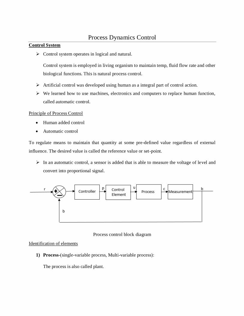
The output variables are also classified as

1. Measured o/p variable:- If there values are known by directly measuring them.

2. Unmeasured o/p variable:-If they are not or can’t be measured directly.

According to their measurability the disturbance are 1) measured, 2) Unmeasured

disturbance.

Design Element of a Control System

Define control objective?

Ensure the stability of the process.

Modeling consideration for control purposes

A chemical process and its associated i/p & o/p

Above model should have the following general form for every output.

Output=f(input variables)

From the above figure, the relationship implies that

Yi=f(mi,m2

Degree of freedom

The degree of freedom of a processing system are independent variables that must be

specified in order to define the process completely.

Desired control of a process will be achieved when and only when all the degree of

freedom have been specified.

The arbitrarily specified variables are the degree of freedom and there is given by

the following relationship.

F=(no.of variables)-(no.of equation)

F=V-E

E:- independent equation i.e differential or algebraic

V=Independent variables

F=no. of degree of freedom

Case:1- if F=0 i.e. V=E;

The solutions of the E equation yields unique values for the V variables.

The process is exactly specified.

Case:2-if F>0 i.e. V>E

Multiple solution result from the E equation specify arbitrary f of the Variables.

The process is under specified.

Case:3-if F<0 i.e.V<E

There is no solution to the E equation.

The process is over specified.

Controller Principle

Process characteristics

1. Process equation

2. Process load

3. Process lag

4. Self-regulation

Process Equation:- A process control loop regulates some dynamic variable in a process.

The controlled variable, a process parameter many other parameter.

If a measurement of the controlled variable shows a variation from the set-point, the

controlling parameter is changed.

TL=F(QA, QB, QS, TA, TS, To)

QA, QB = flow rate in pipe A&B.

QS = Steam flow rate

TA = Ambient Temperature.

To = Inlet fluid Temperature.

TS = Steam Temperature.

Process Load: - The Term Process load refers to set of all parameters, excluding the controlled

variable.

If the set point is changed, the control parameter is attached to cause the variable to adopt new

operating point.

The controlling variable is adjusted to compensate for load change and it effect on the dynamic

variable to bring it back to the set-point.

Transient:- It causes variation of the controlled variable and the control system must take equally

transient change of the controlling variable to keep error to a minimum.

Process Lag:-

Self-Regulation:- A process is said to be self-regulated if a specific value of the controlled variable

is adapted for nominal load with no control action.

Control System Parameters

i. Error (e = r-b) e=error

b=Measured indication of variable

r=set point of variable (reference)

100minmax

min

CC

CCCp

Cp=measured value as % of measurement range

C= Actual measured value

Cmax= Max. of measured value

Cmin= min. of measured value.

100minmax

bb

bre p

Example: A standard measured indication range line 4-20 mA. We have set-point and

measurement range is 10.5 mA & 13.7mA respectively. Find ep.

100420

7.135.10

pe

ep= -20%

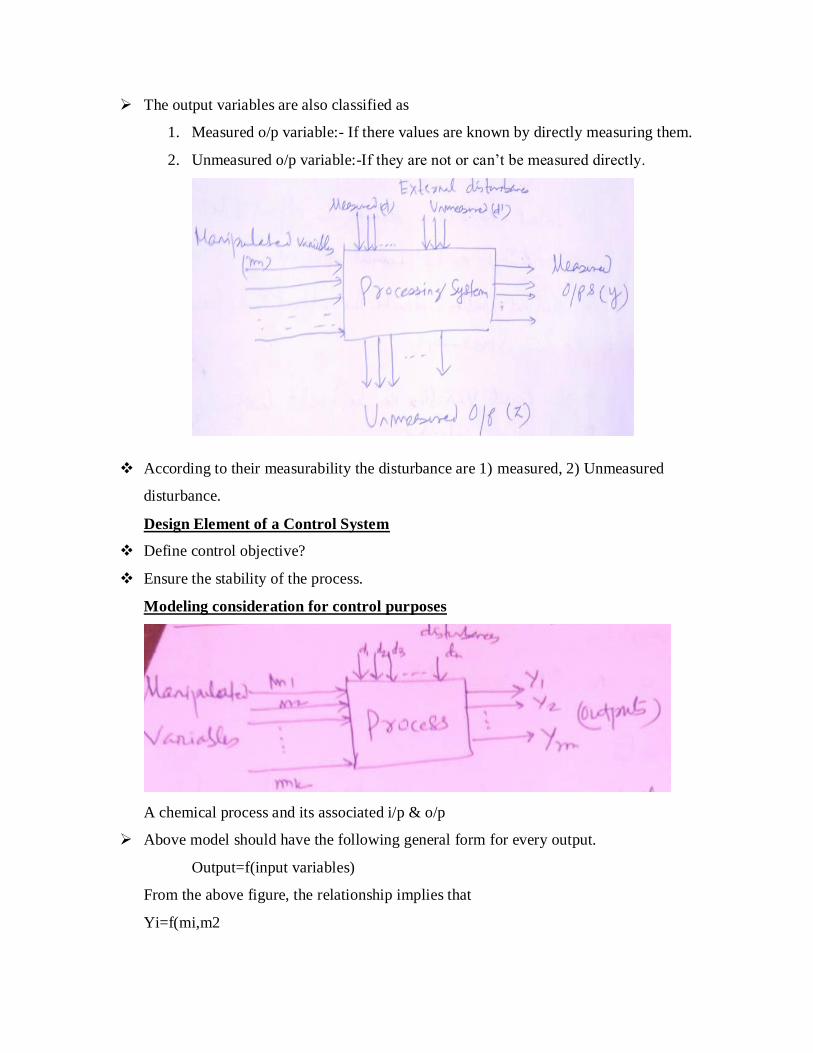
A +ve error indicates a measurement below set-point. And –ve error indicates a

measurement above the set-point.

Self-Regulating System

Non-Self Regulating System

Stable system Unstable system

No need of control action Need control action

No controller is used Controller is required for control action

Pneumatic Signals

The general field of pneumatic covers a broad area of application of gas pressure to

industrial requirements.

Application to provide a force by the gas pressure acting on a piston or diaphragm.

Pneumatic means of propagating information i.e. signal carries and signal can be converted

to other form.

Principle:- In this system, information is carried by the pressure of gas in a pipe.

If we have a pipe of any length & raise the pressure of gas in one end, This increase in pressure

will propagate down the pipe till the pressure throughout is raised to the new value.

The pressure signal travels down the pipe at a speed in the range of the speed of sound in the

gas, which is about 330m/s (1083ft/Sec).

If a transducer varies gas pressure at one end of a 330m (360 yd) pipe in response to some

controlled variable , then that same pressure occurs at the other end of the pipe after a delay of

approx. 1S.

In general, pneumatic signals are carried with air as the gas and signal information are adjusted

to it within the range of 3-15 Psi.

In SI units system, the range (20-100)kPa is used.

Amplification (pneumatic Amplifier)

A pneumatic amplifier is called a booster or relay.

It raises the pressure or air flow volume by linearly proportional amount from the input

signal

If the booster has a pressure gain of 10, the o/p would be 30-150 psi for an input of 3-15

psi

It is accomplished via a regulator that is activated by the control signal.

As the signal pressure varies, the diaphragm motion will move the plug in the body block of

the booster.

If motion is down, the gas leak is reduce and pressure in output line is increased.

High signal produce will cause o/p pressure to decrease.

Nozzle/Flapper System

An important signal conversion is from pressure to mechanical motion & vice-versa. This

system is called nozzle/flapper or nozzle/baffle system.

A regulated supply of pressure, usually 20 psi provide a source of air through the restriction.

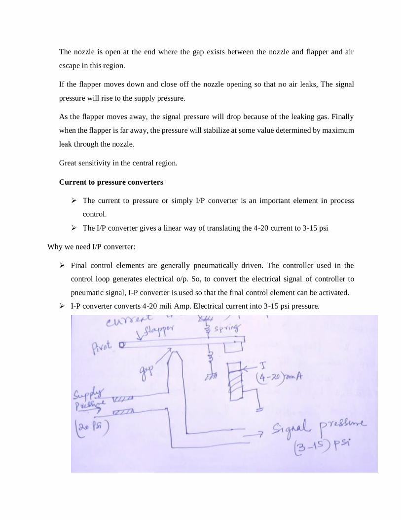
The nozzle is open at the end where the gap exists between the nozzle and flapper and air

escape in this region.

If the flapper moves down and close off the nozzle opening so that no air leaks, The signal

pressure will rise to the supply pressure.

As the flapper moves away, the signal pressure will drop because of the leaking gas. Finally

when the flapper is far away, the pressure will stabilize at some value determined by maximum

leak through the nozzle.

Great sensitivity in the central region.

Current to pressure converters

The current to pressure or simply I/P converter is an important element in process

control.

The I/P converter gives a linear way of translating the 4-20 current to 3-15 psi

Why we need I/P converter:

Final control elements are generally pneumatically driven. The controller used in the

control loop generates electrical o/p. So, to convert the electrical signal of controller to

pneumatic signal, I-P converter is used so that the final control element can be activated.

I-P converter converts 4-20 mili Amp. Electrical current into 3-15 psi pressure.

The current flowing through force coil, produce a force of attraction that pulls the flapper

down to close the air gap between flapper & nozzle.

To obtain a linear transformation of 4-20 mAmp. In to 3-15 psi, The spring assembly is

adjusted with respect to flapper and its relative motion towards the nozzle.

A high current produces a high pressure so that the device is direct acting.

A P-I converter is thus a force balance device in which the coil is suspended in the field of

magnet by a flex core. The relative motion of the flapper is directly proportional to force

exerted by the current carrying coil.

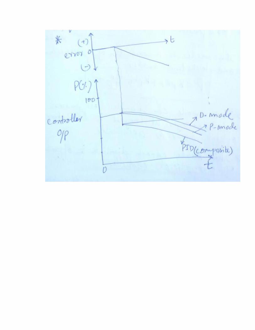
Continuous Controller Modes

In continuous controller modes, the o/p of the controller changes smoothly in response to

the error or rate of change of error .These modes are extension of discontinuous controller

modes.

Proportional Control Mode: The two position mode has the controller o/p of either 100% or

0% , depending on the error being greater or less than the neutral zone.

In multiple step modes, more divisions of controller o/p varies error are developed. This

concept called proportional mode which gives a smooth linear relationship exits between the

controller o/p and the error.

The range of error to cover the 0% to 100% controller output is called the proportional based

as one to one correspondence exist only for error in the range. This mode can be expressed by

P=Kpep+P0

Where Kp= Proportional gain between error are o/p (%/%)

P0= controller output with no error (%)`

Direct and Reverse Action

e = r-b r = set point, b = measurement

if b>r then e= -ve

Then Kp ep will subtract from P0. So equation P=Kpep+P0 represents reverse action.

Direct action would be provided by putting a –ve sign in front of the correction term.

In general, the proportional bend is defined as PB=100/Kp

1. If the error is ‘0’ the output is constant=(P)

2. If There is error, for every 1% of error, a correction of Kp percent is added to or

subtracted from P0, depending on the sign of error.

3. This is a band of error about zero of magnitude PB within the o/p is saturated at 0% or

100%

Offset:- It is an important characteristics in proportional control mode. It produce a permanent

residual error in the operating point of the control variable when change in load occurs. This error

is called offset.

It can be minimized by a larger constant Kp which reduce the Proportional band.

Application: P-controller is used in process where large load changes likely or with moderate to

small process lag time.

If lag time is small, PB is small means Kp is very large which reduce offset error.

Integral-control Mode:-

In proportional control, offset error is present i.e. zero error output is a fixed value. But

integral reduces this problem by allowing the controllable to adapt to changing external

conditions by changing zero order output.

If error makes random excursion above and below zero, net sum will be ‘0’, So there will

be no integral action. But if error becomes +ve or –ve for an extended period of time,

integral action will short and makes changes to controller output.

This mode is represented by

)0()(0

PdteKtP

t

pI

Where P(0)=controller output when integral action starts.

KI =integral gain=It express how much controller o/p in % is needed for every % time

accumulation of error.

The rate at which controller output changes dp/dt=KIep

This equation shows when an error occurs the controller begins to increase (or decrease)

its o/p at a rate which depends upon size of the error and the gain.

If ep=0, no change in controller o/p.

ep= +ve, the controller output begins to ramp up at a rate of dp/di=KIep

This shows how the rate of change of controller output depends upon the value of error and

size of gain.

Characteristics of I-controller

1. If ep=0 o/p remain fixed at a value equal to what it was when the error went to 0.

2. If ep not equal to 0, o/p will begin increasing & decreasing at rate of KI%/sec for every

1% of error.

Integral time or reset action =1/KI

Unit of KI = %/min /% of error

Application of I-controller

Used for system with small process lags and small capacities

Integral mode cant be used alone.

Integral Control Mode

Offset error of P-controller occurs become the controller cannot adopt to change external condition

i.e. changing loads.

Integral controller eliminates offset error

It can be written as

)0()(0

PdteKtP

t

pI Where P(0)=controller output when integral action starts.

KI =integral gain=It express how much controller o/p in % is needed for every % time

accumulation of error.

Integral action is followed by taking the derivative of equation(1).

dp/dt=KI ep

Above equation shows that where error occurs, the controller begins to increase its output at a rate

that depends on the size of the error and gain.

If e=0 The controller output is changed.

If e=+ve the controller output begins to ramp up at a rate by equation.

The rate of change of controller output depends on value of error and the size of the gain.

List the characteristics of the integral mode

1. If the error is zero, the output stays fixed at a value.

2. If the error is not zero, the output will begin to increase or decrease at a rate of K I %/sec

for every 1% of error

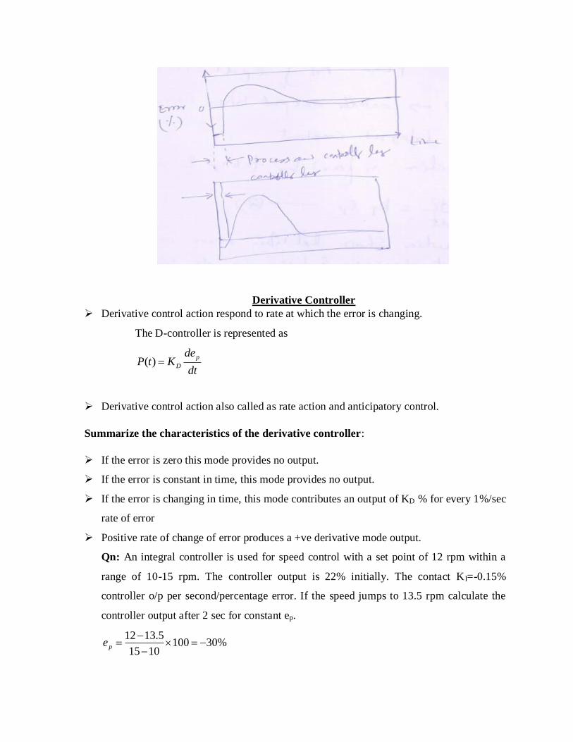
Derivative Controller

Derivative control action respond to rate at which the error is changing.

The D-controller is represented as

dt

deKtP

p

D)(

Derivative control action also called as rate action and anticipatory control.

Summarize the characteristics of the derivative controller:

If the error is zero this mode provides no output.

If the error is constant in time, this mode provides no output.

If the error is changing in time, this mode contributes an output of KD % for every 1%/sec

rate of error

Positive rate of change of error produces a +ve derivative mode output.

Qn: An integral controller is used for speed control with a set point of 12 rpm within a

range of 10-15 rpm. The controller output is 22% initially. The contact KI=-0.15%

controller o/p per second/percentage error. If the speed jumps to 13.5 rpm calculate the

controller output after 2 sec for constant ep.

%301001015

5.1312

pe

Integral Mode

The rate of controller output is proportional to the error. Integral controller is also called as

reset controller.

If the error is nonzero the integral action will cause the value of manipulated variable to

change.

The controller output is not only a function of the duration of the error.

The equation of I-controller is

p

i

pi ET

EKdt

dp 1

0)()( PdttEKtP pi

P(t) is the controller o/p at time t.

P0 controller output at time t=0 & dp/dt=is the rate at which the control output changes

(%/s)

Ep is the error.

KI is rate of controller output in %/min/%error

Controller output is limited by the maximum permissible controller o/p (100%)

Qn: An integral mode controller with reset time of 6 min . find the Ki.

Ans:- 1/6*60=2.77mSec-1

If the error=0, o/p stays fixed at a value of controller when it ……zero.

If error not equal, o/p will begin to increase or decrease at the rate of Ki%/s for every 1%

error.

Unlike proportional controller, I-controller do not produce offset.

Ki express in %change/min/%error

Characteristics of I-controller

No error at steady state (No-offset)

Sluggish response at high Ti (reset time)

At small Ti, the control loop tends to oscillate (control loop may become unstable)

Derivative Mode

It is known as rate mode/predictive mode/anticipatory mode. The controller o/p in

derivative mode is proportional to the rate of error.

D-controller genetic the manipulated variable from the rate of change of error, unlike P-

controller which generates manipulated variable from the amplitude of error.

The equation of D-controller

0)( Pdt

dEKtP

p

d

Kd= Derivative gain constant in (%(%/sec))

dep/dt= rate of change of error in (%/sec)

Derivative action is used primarily in process with long dead and lag times.

D-controller has no effect on the o/p if the error is not changing. So, it cannot be

used alone. This is an anticipating action that may contribute to the inherent

instability of fast acting control loops

Application

The derivative mode cannot be used alone since when the error is zero or constant,

the controller has no output.

If the error is changing with time, the derivative mode contributes an output Kd%

for every 1% sec rate of change of error.

Used when the dead time is very larde

Comparison among P, I & D controller

Mode Benefit Drawback

P 1. Rapid adjustment of

manipulated variables

2. Speeds Dynamic

response

1.Non-zero offset

2.Can cause instability

I 1.Produce zero offset 1.slow dynamic response

2.can cause instability

D Provide rapid response to

control variable changes

1.non-zero offset

2.Sensitive to noise in

controlled variable.

Discontinuous Controller Mode

It shows discontinuous changes in controller o/p as controlled variable error occurs.

Two position Mode:

The elementary controller mode is ON/OFF or two position mode. This is discontinuous

mode controller.

It is simplest and cheapest

An analytical equation cannot be written

We can write

0% Ep<0

P= 100% Ep>0

When the measured value is less than set point, full controller output.

When it is more than set point, the controller output is zero.

If the temperature drops below the set point, the heater is turned ON. If the temp.

rises above the set point, it turns OFF.

Neutral Zone

Application:

The two position control mode is best adapted to large scale system with relatively slow

process rate . Example:- Room heater, AC

Two position control application are liquid bath-temp. control and level control in large

volume tank.

Multi-position Mode

A logical extension of two position control mode is to provide several intermediate, rather

than only two, settings of the controller o/p.

This discontinuous control mode is based in an attempt to reduce the cycling behavior, &

overshoot, undershoot inherent in two position controller mode.

This mode is represented as

P= Pi ep > [ei ] i=1, 2, 3……n

As the error exceeds certain set limits +/- ei, the controller output is adjusted to protect values Pi

Common example of three position controller

Error in between E2 & E1 of the set point, the controller stays at some nominal setting

indicated by a controller output of 50%.

If the error exceeds the set point by E1 or more, than the o/p is increased by 100%.

If it is less than the set-point by –E1 or more, the controller o/p is reduced to zero.

100 Ep>E2

50 -E1<Ep<E2

P= 0 Ep<-E1

Floating Mode Controller

If the error exceeds some preset limit, the output was changed to a new setting as soon as

possible.

In floating control, the specific output of the controller is not uniquely determined by the

error.

If the error is zero, the output does not change but remains (floats) at whatever setting it

was when the error went to zero.

Actually with two position controller mode, this is typically a neutral zone around zero

error where no change in controller position occurs.

Single Speed

In single speed floating mode controller, the o/p of the control element changes at a

fixed rate when exceeds the neutral zone.

For single speed control dp/dt=+/-KF ep>𝞓 ep

Where dp/dt= rate of change of controller o/p with time

KF= rate constant %/s

𝞓 ep = half the neutral zone.

If the above equation is integrated for the actual control output, So we get

P=+/- KFt+P(0) ep> 𝞓 ep

Where P(0) = controller output at t=0

Actual value of P floats at an undetermined value.

Multiple Speed

In floating multiple speed, several possible speeds(rates) are changed by controller output.

FiKdt

dp ep> epi

If the error exceeds epi, Then speed of KF1

If the error rises to exceed ep2 the speed increase to KF2 and so on

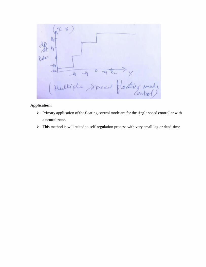
Application:

Primary application of the floating control mode are for the single speed controller with

a neutral zone.

This method is will suited to self-regulation process with very small lag or dead-time

Composite Control Mode

By combining several basic mode, advantages of each mode can be achieved in composite

control mode.

The composite control modes tend to eliminate some limitations they individually possess.

3-types of composite control modes

1. PI controller 2. PD controller 3. PID controller

Proportional-Integral control(PI):

This is a control mode that results from a combination of proportional mode and the integral

mode.

It can be represented as

t

IpIPpp PdteKKeKP0

)0(

Where PI(0)= integral term value at t=0

Advantage of PI-mode is that one-to-one correspondence of the P-mode is available and integral

mode eliminates the inherent offset.

P-mode introduce a offset error when a load change occurs. The integral function provides the

required new controller o/p thereby allowing the error to be zero after a load change.

Characteristics of PI control mode:

When pe =0, controller output is fixed at the value that the integral term had when error

went to zero.

If pe not equal to zero The proportional term provide a correction and the integral term

begins to increase or decrease the accumulated value. Depending on the sign of error and

the direct or reverse action.

Applications:

This mode can be used in systems with frequent or large load changes.

Disadvantages:

The process must have relatively slow change in load to prevent oscillations induced

by integral overshoot.

During start-up of a process, integral action causes overshoot of errors and output,

before settling to operating point.

In this mode PB is constant but its location is shifted as the integral term changes.

Proportional-Derivative Controller (PD):

This mode is a combination of proportional and derivative modes

0Pdt

deKKeKP

p

DpPP

This mode can handle fast process load changes as long as the load change offset error is

acceptable.

This mode cannot eliminate the offset error of proportional controller.

This mode is generally used for industrial application.

Three mode (PID) controller:

This mode operations combines the proportional integral and derivative modes.

It is a powerful and complex controller mode.

This mode can be expressed as

)0(0

I

p

Dp

t

pIPPP Pdt

deKKdteKKeKP

This mode eliminates the offset of the proportional mode and also provide fast response.

Different Types of Actuators

Actuators take on many forms to suit particular requirement of process control loop

3-types of actuator

1. Electrical Actuator

2. Pneumatic Actuator

3. Hydraulic Actuator

Electrical Actuator:

A. Solenoid:

Solenoid converts an electrical signal in to mechanical motion (rectilinear motion).

It consists of a plunger and a coil. The plunger may be free standing or spring loaded.

Specification of solenoid include electrical rating and the plunger push pull force.

Solenoids are used are used when a large & sudden force applied to perform some job.

B. Electrical Motors:

Electrical motor converts electrical input into continuous mechanical rotation.

Electrical motor operates through interaction of magnetic fields and current conductor to

generate force.

In this motor, moving part is called rotor and stationary part is called stator.

DC Motors

DC motor is powered by direct current and the rotation is produced by the interaction of

two constant magnitude field.

DC motor has a permanent magnet to form one magnetic field. Second magnetic field is

formed by pacing a current.

Compound Field:

High starting torque

Good speed control

AC Motors:

Rotation is produced by interaction between two magnetic fields & both fields are

varying in time in consonance with a.c excitation voltage. The force between fields

is a function of angle of rotor and phase of current pacing through coil.

AC motors are 2 types

1. Synchronous Motor

2. Induction Motors

Synchronous AC motors:

Through a coil contained within the permanent magnet field. As there exist a torque in armature,

rotation continue and the speed depends on the current.

Series field:

Large starting torque.

Difficult to control speed.

Good in for starting heavy, no mobile loads where speed is not important.

Shunt field:

Smaller starting torque.

Good speed control.

AC voltage is applied to field coil and starter. The magnetic field is varying with time and

phase of input voltage. The armature called rotor is either permanent magnet or dc

electromagnet.

In this motor, rotor follows the AC magnetic field of stator.

The speed of rotation given by ns

ns=120f/p (rpm)

where f-excitation frequency

p- no. of poles

The motor provides lower starting torque and low power when operated using single phase

a.c when operated with 3-phase, they provide very high power.

Induction AC Motor

Rotor is either PM or dc excited electromagnet current induced in the coil that wounded

over rotor, generates interacting magnetic fields of rotor. The current is induced from stator

coil.

AC field of stator produce a changing magnetic field which passes through closed loop of

rotor. Due to changing flux a current is induced in rotor loop and generate magnetic field

of rotor. There exist a torque on rotor due to two magnetic field.

Stepping Motor:

Stepping motor can be interfaced with digital circuit.

It is a rotating machine that completes a full rotation through series of discrete rotational

steps.

Continuous rotation is achieved by the i/p of a pulse train. The rotational rate is determined

by the no of steps per revolution and rate at which pulse are applied.

A change in i/p current from one step to another creates a single step change in rotor

position.

If the phase current state is not changed the rotor position stay in that stable position.

C. Pneumatic Actuators

Pneumatic actuator converts energy (typically in the form of compressed air) into

mechanical motion. The motion can be linear or rotary depending upon type of actuator.

In this spring & diaphragm actuator variable air pressure is applied to a flexible

diaphragm to oppose spring attached to it.

The pressure on the spring side of diaphragm is maintained at atmospheric pressure by

the open hole.

Increase in control pressure i/p pressure applies a force on the diaphragm to force the

same to push down the shaft connected to it against the spring force.

The basic principle of actuator is based on the concept of pressure as force per unit

area. When net pressure difference is applied across a diaphragm of surface area A,

then net force acts on the diaphragm is given by

F=A(P1-P2)

Where P1-P2=Pressure diff (in Pa)

A=diaphragm area(m2)

F= force (in N)

Force can be double by doubling the diaphragm area.

𝞓x=A/K *𝞓P

Where 𝞓x=shaft travel (m)

𝞓P=applied pressure (Pa)

A=diaphragm area(m2)

K=spring constant. (N/m)

Reverse acting pneumatic actuator:

Reverse actuator pull the shaft inside or towards the spring when input pressure is applied.

Shaft travel is maximum when no. pressure is applied.

D. Hydraulic Actuator

In pneumatic actuator, there is a upper limit of force that can be applied. To overcome this

hydraulic actuator is used.

In hydraulic actuator, incompressible fluid is used to provide the pressure.

PH=F1/A1

Where PH=Hydraulic pressure (Pa)

F1=applied piston force (N)

A1=Forcing piston area(m2)

The pressure can be made very large by adjusting the area of the forcing piston.

This pressure is transferred equally through out the liquid, so the resulting force on working

piston is FW=PHA2, where FW is force on working piston, A2 is working piston area.

The working force is given by in terms of the applied force.

Control System Components

Control Valve:

Control valve is a device by which the flow of fluid may be started, stopped or regulated

where a movable part opens or obstructs passage.

4 main functions of control valve

1. Start and stop flow

2. Regulation of flow

3. Back flow prevention

4. Release pressure

Control Valve Principle:

Flow rate is generally expressed in volume per time. If a given fluid is delivered through a

pipe, then the volume flow rate is Q=AV.

Q=flow rate (m2/s), A=Pipe Area (m2)

V= flow velocity (m/sec)

Control valve regulate the flow rate of fluid by placing a variable size restriction in the

flow path.

As the stem & plug move & down, the size of opening between the plug and seat changes

there by changing the flow rate. There will be a drop in pressure across such a restriction

& the flow rate varies with square root of this pressure drop.

Q=K P

Where K=proportional constant (m3/sec/pa)

𝞓P=P2-P1 pressure difference

Control Valve Characteristics:

Control valve characteristic shows the relationship between valve opening & flow rate

under constant pressure condition.

There is an assumption that the stem position indicate the extent of valve opening & the

pressure difference is determined by the valve body.

There are 3 basic types of control valve. The types of valves are determined by the shape

of plug & seat of valve.

1. Quick Opening

2. Linear Valve

3. Equal percentage valve

Quick Opening Valve:

This type of valve is used for full ON or full OFF control application.

In this valve a relatively a small motion of valve stem results in maximum possible flow

rate through the valve i.e. 90% of maximum flow rate is achieved with only a 30% travel

of the stem or valve opening.

The valve opening is linear up to 60-70% of the valve opening. After this limit Flow does

not change rapidly with change in the valve opening.

Linear Valve:

The flow is directly proportional to the valve opening for a constant pressure drop.

The relationship is expressed as

maxmax S

S

Q

Q Where Q= flow rate (m3/s)

S= Stem position (cm)

Equal Percentage:

Equal percentage increment in valve position/stem position produces an equivalent change

in flow.

The type of valve does not shut off completely in its limit of the stem level

Qmin=minimum flow when the stem is at one limit of its travel.

Qmax=maximum flow where the stem is at other extreme

Rangeability = Qmax/ Qmin = Cvmax/Cvmin

The curve shows that the increase in flow rate for a given change in valve opening depend

on the extent to which the valve is already open.

Q=QminmaxS

S

R

Rangeability:

It is the ratio of max controllable flow to minimum controllable flow.

Control Valve Sizing:

Valve size is chosen by the flow that value can provide & the nominal size of the end

connection.

Control valve sizing involves determining the correct valve to install from many valves.

Control Valve Sizing

Valve size is chosen by the flow that valve can provide & the nominal size of the end

connection.

Control valve sizing involves determining the correct valve to install form many valves.

The process of valve choosing is based on the information about the capacity of values,

which can be known from value co-efficient.

Cv= Valve co-efficient that define max capacity of a value.

Cv is defined as the number of gallon per min of water that flow through a fully open valve

with a pressure drop of 1 psi.

Rules for Selecting Valve Characteristics

1. Equal percentage

o Used in process where large change in pressure drop are expected.

o Used in process where a small percentage of total pressure drop is permitted by the

valve.

o Used in temperature and pressure control loop.

2. Linear

o Used in liquid level or, flow control.

o Used in system where the pressure drop across the valve is expected to remarking

fairly constant.

3. Quick opening

o Used for frequent on-off service

o Used for process where instantly large flow is needed.

Eg. Safety system or, cooling water system.

Ball Valves

Ball valves are stop valves that use a ball to stop or, start the flow of fluid.

Where the valve handle is turned to open the valve, the ball rotates to a point such that the

entire hole through the ball is in line with valve body.

As a result, fluid starts flowing through the valve.

When the ball is perpendicular to the flow openings of valve body the valve is shut off.

These valve are generally quick opening types and can be linear.

Globe Valve

Globe valves are linear motion valves with round bodies. The valve body is of globular

shape.

These valves are widely used in industry to regulate fluid flow in both on-off and throttling

service.

Globe valves are generally two port valves. Ports are the opening in the body to let the

water flow in or, out. Globe valves with ports at an angle called angle globe valves.

Two types of Globe valves.

Single Port

Double Port

Single port Valves are used for application with stringent shut of requirements.

Double port Globe valve is commonly used as fully open or, fully closed. They have higher

capacity than single port valve and used in larger pipe size.

Limitations of Globe Valve

The globe valve should never be jammed in open position. After the valve is fully open,

the hand wheel should be turn towards the close position. Otherwise the valve will seize

in open position and it is difficult or, impossible to close the valve.

Globe valves are linear and equal percentage type.

Introduction to Feed-Back Control

Concept of feed-back control

The disturbances (d) [known as load or, process load] changes in an unpredictable

manner and our control objective is to keep the value of the output at desire value.

A feed-back control system works in the following manner.

Measures the value of the output using the appropriate measuring device. Here ym be the

value that indicated by the measuring sensor.

Compare ym to desired value ysp of the output. Here the deviation error e= ysp-ym.

The value of error is supplied to the main controller. The controller changes the

manipulated variable m in such a way as to reduce the magnitude of the deviation e.

The controller affects the manipulated variable through another device (usually a control

value), known as the final control element.

Example of feed-back control system

1) Flow control

2) Pressure control

3) Temperature control

4) Composition Control

5) Liquid level Control

Basic hardware component of feed-back control system

1) Process- Takes, heat exchange, reacts, Separates etc.

2) Measuring instruments or, sensor- Thermocouples, bellows, diaphragm, orifice plate.

3) Transmission lines- Used to carry the measurement signal from the sensor to the

controller and control signal from the controller to the final control element.

4) Controller- It takes the error input and minimize the error through several processes.

5) Final control element- It is the controller output given to a actuator to control the process.

Types of feed-back controller

e(t) = ysp(t)-ym(t) output= c(t)

Continuous controller differs by relating with e(t) to c(t).

Output signal of a feed-back controller depends on its constructions and may be a

pneumatic signal for pneumatic controller or, an electrical one for electronic

controller.

Three types of feed-back controller P, PI, PID.

Proportional controller

A proportional controller is designed by the value of its proportional gain or equivalently

by its proportional band where PB = 100/Kp.

The proportional band characteristics the range over which the error must change in order

to drive the actuating signal of the controller over it full range.

The larger the gain Kp, the smaller the proportional band, the higher the stability.

Proportional-Integral Controller

It is mostly known as proportional reset controller.

Reset time constants are adjustable.

Reset time is the time needed by the controller to repeat the initial proportional action

change in its output.

Integral controller eliminates small errors.

PID Controller

Industrial practice it is known as Proportional-Reset-Rate Controller.

The output of this controller is given by:

In the presence of de/dt , the PID controller anticipates what the error will be in the

immediate future.

Derivative control action is known as anticipatory control.

Draw-backs of the Derivate control action

For a response with constant non-zero error it gives no control action since de/dt=0.

For a noisy error with almost zero error it can compute large derivative and this yield

large control action.

Measuring Devices and sensors.

Measured Process Variable Measuring Devices

Temperature Thermocouple, RTD, Thermistor,

Radiation Pyrometer, gas filled

Thermometer, Oscillating quartz

crystal.

Pressure Manometer, Burden tube, bellows,

diaphragm, strain gauge.

Flow Orifice plate, rota meter, Venturi

meter, turbine flow meter, Ultra sound,

Hot wire anemometer.

Liquid Level Float, Displacer device, Dielectric

measurement, Sonic resonance.

Composition PH meter, Spectrometer,

Chromatographic analyzer, Ir UV

Visible radiation analyzer

ADAPTIVE CONTROL

To adapt means to change the behavior to fit to new circumstances.

An adaptive controller is a controller that can modify its behavior in response to changes

in the dynamics of the process and the character of the disturbances.

In 1961, a long discussion ended with the suggestion. An adaptive system in any physical

system that has been designed with an adaptive view point.

In 1973, an IEEE committee proposed the self-organizing control (SOC) system, parameter

adaptive SOC system, performances adaptive SOC and learning control system.

An adaptive controller is a controller with adjustable parameters and a mechanism to adjust

those parameters

The controller becomes nonlinear due to the parameter adjustment mechanisms.

An adaptive control system can be thought of as having two loops. One is with normal

feedback with the process and the controller while the other is the parameter adjustment

loop.

ADAPTIVE SCHEMES

Four types of adaptive schemes :

1. Gain scheduling

2. Model reference adaptive control

3. Self-tuning regulations

4. Dual control

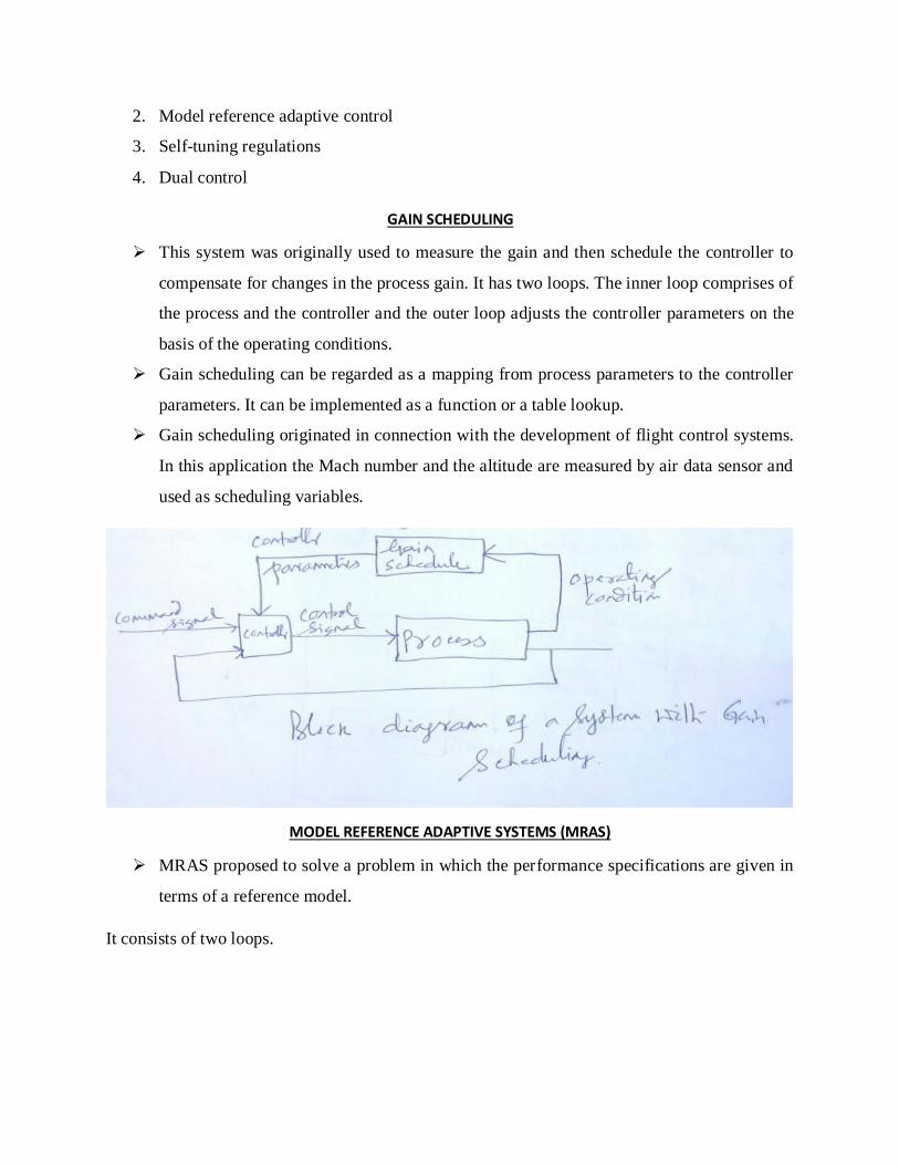
GAIN SCHEDULING

This system was originally used to measure the gain and then schedule the controller to

compensate for changes in the process gain. It has two loops. The inner loop comprises of

the process and the controller and the outer loop adjusts the controller parameters on the

basis of the operating conditions.

Gain scheduling can be regarded as a mapping from process parameters to the controller

parameters. It can be implemented as a function or a table lookup.

Gain scheduling originated in connection with the development of flight control systems.

In this application the Mach number and the altitude are measured by air data sensor and

used as scheduling variables.

MODEL REFERENCE ADAPTIVE SYSTEMS (MRAS)

MRAS proposed to solve a problem in which the performance specifications are given in

terms of a reference model.

It consists of two loops.

The key problem with MRAS is to determine the adjustment mechanisms so that a stable

system, which brings the error to zero, is achieved. This problem is non-trivial.

Parameter adjustment mechanism called MIT rule was used in the original MRAS.

MIT rule can be regarded as a gradient scheme to minimise the squared error e2.

SELF TUNING REGULATORS

A different scheme is obtained if the estimates and the process parameters are obtained

from the solution of design problem using the estimated parameters

It has two loops. (Inner loop and outer loop)

The parameters of the controller are adjusted by the outer loop which is composed of a

recursive parameter estimator and a design calculation.

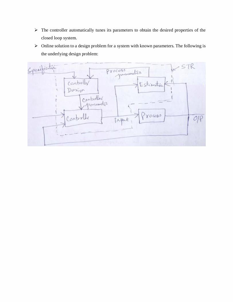
The controller automatically tunes its parameters to obtain the desired properties of the

closed loop system.

Online solution to a design problem for a system with known parameters. The following is

the underlying design problem:

PLC

Programmable logic controller, commonly known as PLC.

It is solid state digital industrial computer.

In 1968, it was conceived by group engineers, from General Motors.

To replace sequential relay circuits, which are mainly used for machine tool, PLC was invented.

Microprocessor based PLCs were introduced in 1977 by Allan – Bradley in USA.

PLCs are designed to work in hostile environments of industries and replaced hardware relays,

discrete electronic components circuitry to realize sequential logical and analog controls in

industries.

According to NEMA (National Electrical Manufacturers Associations, USA) the definition of PLC

is---

“Digital electronic device that uses a programmable memory to store instructions and to implement

specific functions such as logics, sequencing, timing, counting and arithmetic to control machines

and processes.”

APPLICATIONS OF PLC

In automation, field of sequence control

Motor control, process control, data management and communication systems

Machine control, material handling, sequence control

PLCs can provide information about alarm limit detection, alarm messages, machine malfunction,

productive summary, machine status etc.

BASIC PARTS OF PLC

All programmable controllers, contain a CPU, memory, power supply, I/O modules and

programmable devices. The basic parts include:

1. Processor

2. Memory

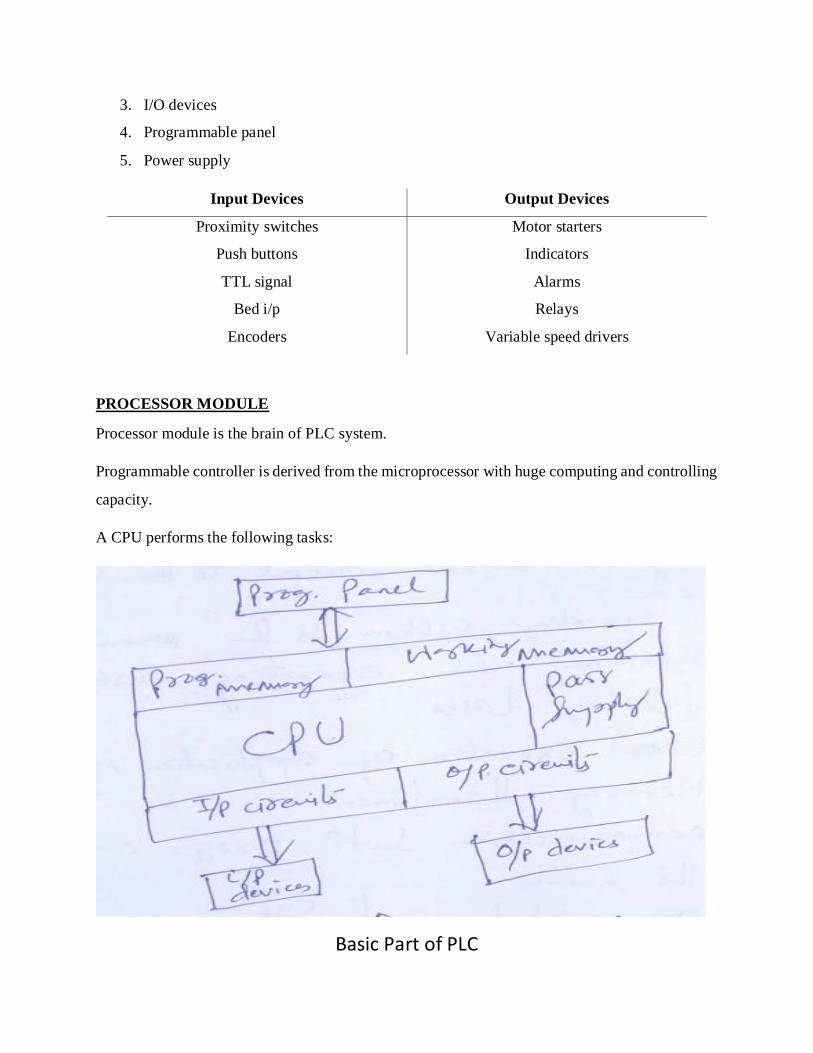
3. I/O devices

4. Programmable panel

5. Power supply

Input Devices Output Devices

Proximity switches Motor starters

Push buttons Indicators

TTL signal Alarms

Bed i/p Relays

Encoders Variable speed drivers

PROCESSOR MODULE

Processor module is the brain of PLC system.

Programmable controller is derived from the microprocessor with huge computing and controlling

capacity.

A CPU performs the following tasks:

Basic Part of PLC

1. Scanning

2. Program execution

3. Peripheral and external device communication

4. Self-diagnostics

Power of programming controller depends on the type of microprocessor used. Small size

programming controller uses 8-bit microprocessor.

The job of the processor is to monitor the state of the i/p devices, scan and solve the logic of a

user program and provide analog or discrete output to the output devices.

The operating system is the main workhouse of the system. The operating system performs the

following tasks.

1. Execution of application program

2. Memory management

3. Communication between program controllers and other units.

4. i/o interface handling

5. Diagnostics

6. Resonance sharing

The OS is stored in a non-volatile memory as the ROM whereas the application programs are

stored in RWM (Read-Write Memory).

INPUT MODULES

Different types of i/p modules. i/p modules used is dependent on the kind of real world inputs

the PLC is required to handle.

Nature of i/p can broadly be classified into 3 types:

1. Analog/Digital (two bit/ multi bit)

2. Low / High frequency

3. Maintained or momentary

4. 5V/24V/110V/220V switches

Typical-8 to 32 input points ,Output Module-6 to 32 output points on single module