Process Analytical Technology (PAT) and Quality by Design (QbD)

Chapter 18Process Analytical Technology (PAT)

and Quality by Design (QbD)

Multi- and Megavariate Data Analysis

Basic Principles and Applications

Third revised edition

L. Eriksson, T. Byrne, E. Johansson, J. Trygg and C. Vikström

Value From Data

®

1 Introduction2 Basic concepts and principles of projections3 PCA4 PLS5 Orthogonal PLS (OPLS)6 O2PLS7 Multivariate characterization8 Multivariate calibration9 Multivariate process modeling10 Classification and discrimination11 Identification of discriminating variables12 Transformation and expansion13 Centering and Scaling14 Signal correction and compression15 MSPC16 BSPC17 Multivariate time series analysis

18 Process Analytical Technology (PAT) and Quality by Design (QBD)19 Hierarchical modeling20 Non-linear PLS modeling21 Hierarchical cluster analysis, HCA22 PLS-TreesAppendix I: Model derivation, interpretation, and validationAppendix II: Statistics

This is an extract of chapter 18 from “Multi- and Megavariate Data Analysis”, third revised edition (2013)

Multi- and Megavariate Data Analysis - Ch 18 Process Analytical Technology (PAT) and Quality by Design (QBD) 323

18 Process Analytical Technology (PAT) and Quality by Design (QBD)

18.1 Objective This chapter introduces the concepts of Process Analytical Technology (PAT) and Quality

by Design (QBD) and discusses their merits and possibilities within the pharmaceutical

industry. PAT is founded on chemometric cornerstones like multivariate data analysis

(MVDA), multivariate statistical process control (MSPC) and batch statistical process

control (BSPC). A major benefit of PAT is that of using multivariate process data to provide

more information and a better understanding of manufacturing processes than conventional

approaches (such as univariate SPC). Another benefit is the reduction of idle time at the end

of a process step when product is often held awaiting laboratory results. This second benefit

is a concept called “parametric release”. QBD is founded on similar tools to PAT, but in

addition emphasizes the need for design of experiments (DOE) to achieve trustworthy

results. A major benefit of QBD is the development of a sound scientific basis for a process

design space that accommodates a range of defined variability in commercial process

materials and operations and still produces the right product quality outcomes.

18.2 Introduction In Chapters 15 – 17 we have seen how tools for multivariate data analysis (MVDA) and

multivariate statistical process control (MSPC) form an integrated framework for process

modeling, monitoring and optimization. Using this framework, processes that are running in

a sub-optimal way can be better characterized and understood, and eventually be brought

into a better state of control and maintenance. In this chapter, the objective is to deepen the

discussion on process modeling, monitoring and optimization with special attention to the

influence arising from regulatory activity and guidance. To this end, we shall consider two

concepts denoted PAT and QBD. PAT is short for process analytical technology and QBD

is short for quality by design. The utility of QBD and PAT is well documented in literature

[Andersson, et al., 2005; Luukkonen, et al., 2008; Altan, et al., 2009; Streefland, et al.,

2009; Laursen, et al., 2010; Peterson, 2010; Wu, et al., 2011; Xu, et al., 2012; Kawabe, et

al., 2013; Macedo, et al., 2013; Rozet, et al., 2013].

18.2.1 The PAT initiative

PAT has its origins in an initiative of the US Food and Drug Administration, FDA, first

launched in mid-2002. The goal of PAT is to improve the understanding and control of the

entire pharmaceutical and biopharmaceutical manufacturing process. One way of achieving

this is through timely measurements of critical quality and performance attributes of raw

and in-process materials and processes, combined with multivariate data analysis (MVDA).

This needs to be coupled with Design of Experiments (DOE) to maximize the information

content in the measured data. A central concept within the PAT paradigm is that quality

should arise as a result of design-based understanding of the processes, rather than merely

by aiming to generate products that meet minimum criteria within defined confidence limits,

and rejecting those that fail to meet the criteria.

There are many objectives associated with the PAT concept, but the foremost goal is to

improve the understanding and control over the entire pharmaceutical or biopharmaceutical

324 Ch 18 Process Analytical Technology (PAT) and Quality by Design (QBD) - Multi- and Megavariate Data Analysis

manufacturing process. Briefly, PAT can be understood as a framework of tools and

technologies for accomplishing this goal. Interestingly, the US FDA defines process

understanding as: “the identification of critical sources of variability, management of this

variability by the manufacturing process, and the ability to accurately and reliably predict

quality attributes”. MVDA tools are clearly needed to achieve this, together with insight,

process knowledge, and relevant measurements.

A common question is “what can be accomplished with PAT?” The answer to this is multi-

faceted. In part, this is because PAT means different things to different people. Its answer

may also depend on whether one is involved in academia, industry or a regulatory agency.

Moreover, the connotations associated with PAT depend to a great extent on the context,

e.g. whether it is to be applied to an existing process (continuous or batch) or a process still

under development.

MVDA and PAT may be applied to important unit operations in the pharmaceutical

industry. In our experience, the most common applications of PAT relate to on-line

monitoring of blending, drying and granulation steps. Here, the measurement and analysis

of multivariate spectroscopic data are of central importance. These spectroscopic data form

the X-matrix, and if there are response data (Y-data), the former can be related to the latter

using PLS or OPLS to establish a multivariate calibration model (a so called soft sensor

model). However, MVDA should not be regarded as the only important approach; DOE

should also be considered. DOE is very useful for defining optimal and robust conditions in

such applications.

18.2.2 What are the benefits of using DOE?

DOE is complementary to MVDA. In DOE, the findings of a multivariate PCA, PLS, OPLS

or O2PLS model are often used as the point of departure because such models highlight

which process variables have been important in the past. Systematic and simultaneous

changes in such variables may then be induced using an informative DOE protocol. In

addition, the controlled changes to these important process factors can be supplemented

with measurements of more process variables which cannot be controlled. Hence, when

DOE and MVDA are used in conjunction, there is the possibility of analyzing both designed

and non-designed process factors at the same time, along with their putative interactions.

This allows us to see how they jointly influence key production attributes, such as the cost-

effectiveness of the production process, and the amounts and quality of the products

obtained.

Generally, DOE is used for three main experimental objectives, regardless of scale. The first

of these is screening. Screening is used to identify the most influential factors, and to

determine the ranges across which they should be investigated. This is a straightforward

aim, so screening designs require relatively few experiments in relation to the number of

factors. Sometimes more than one screening design is needed.

The second experimental objective is optimization. Here, the interest lies in defining which

approved combination of the important factors will result in optimal operating conditions.

Since optimization is more complex than screening, optimization designs demand more

experiments per factor. With such an enriched body of data it is possible to derive quadratic

regression models.

The third experimental objective is robustness testing. Here, the aim is to determine how

sensitive a product or production procedure is to small changes in the factor settings. Such

small changes usually correspond to fluctuations in the factors occurring during a “bad day”

in production, or the customer not following the instructions for using the product.

The great advantage of using DOE is that it provides an organized approach, with which it

is possible to address both simple and tricky experimental and production problems. The

experimenter is encouraged to select an appropriate experimental objective, and is then

guided through devising and performing an appropriate set of experiments for the selected

objective. It does not take long to set up an experimental protocol, even for someone

unfamiliar with DOE. What is perhaps counter-intuitive is that the user has to complete a

whole set of experiments before any conclusions can be drawn.


The rewards of DOE are often immediate and substantial, for example higher product

quality may be achieved at lower cost, and with a more environmentally-friendly process

performance. However, there are also more long-term gains which might not be apparent at

first glance. These include a better understanding of the investigated system or process,

greater stability, and greater preparedness for facing new, hitherto unforeseen challenges.

18.2.3 QBD and Design Space

The importance of DOE to the pharmaceutical and biopharmaceutical industry is underlined

by the growing interest in the Quality by Design (QBD) concept inspired by ICH. ICH, the

International Conference on Harmonization of Technical Requirements for Registration of

Pharmaceuticals for Human Use, is a collaborative body bringing together the regulatory

authorities and pharmaceutical industry of Europe, Japan and the US to discuss scientific

and technical aspects of drug registration. ICH's mission is to achieve greater harmonization

to ensure that safe, effective, and high quality medicines are developed and registered in the

most resource-efficient manner. ICH regularly releases guidance documents relating to

quality, safety and efficacy. A number of guidelines on the Quality side, denoted ICH Q8,

Q9 and Q11 (Q for Quality), concern methods and documentation principles of how to

describe a complex production process or analytical system.

The ICH guidance documents position QBD based on DOE as a systematic strategy of

addressing pharmaceutical development. It should be appreciated that it is both a drug

product design strategy and a regulatory strategy for continuous improvement. QBD is

based on developing a product that meets the needs of the patient and fulfils the stated

performance requirements. QBD emphasizes the importance of understanding the influence

of starting materials on product quality. Moreover, it also stresses the need to identify all

critical sources of process variability and to ascertain that they are properly accounted for in

the long run.

As mentioned above, the major advantage of DOE is that it enables all potential factors to

be explored in a systematic fashion. Let us take, as an example, a formulator, who will be

operating in a certain environment, with access to certain sets of equipment and raw

materials that can be varied across certain ranges. With DOE, the formulator can investigate

the effect of all factors that can be varied and their interactions. This means that the optimal

formulation can be identified, consisting of the best mix of all the available excipients in

just the right proportions. Furthermore, the manufacturing process itself can be enhanced

and optimized in the same manner. When the formulation recipe and the manufacturing

process have been screened, optimized and fine-tuned using a systematic approach based on

DOE and MVDA, issues such as scale-up and process validation can be addressed very

efficiently because of the comprehensive understanding that will have been acquired of the

entire formulation development environment.

Thus, one objective of QBD is to encourage the use of DOE. The view of this approach is

that, once appropriately implemented, DOE will aid in defining the design space of the

process. The design space of a process is the largest possible volume within which one can

vary important process factors without risking violation of the specifications (the demands

on the responses). Outside this window of operation, there can be problems with one or

more attributes of the product.

18.2.4 MVDA/DOE is needed to accomplish PAT/QBD in Pharma

Because the pharmaceutical and biopharmaceutical industry has complex manufacturing

processes, MVDA and DOE have great potential and applicability. Indeed, the

pharmaceutical sector has long been at the forefront of applying such technology. However,

this has mainly been at the laboratory and pilot plant scale and has historically been much

less widespread in manufacturing. The main explanation for this dichotomy is that the

pharmaceutical industry has been obliged to operate in a highly regulated environment. This

environment has reduced the opportunity for change which in turn has limited the

applications of MVDA and DOE in manufacturing.


A change to this approach involves confidence in making changes, and those changes must

be based on process and product understanding. The objective in modeling and analysis of

these data is to develop process understanding. The FDA guidance on process analytical

technology (PAT) provides four types of tools for generation and application of process

understanding, including

multivariate tools for design, data acquisition and analysis;

process analyzers;

process control tools, and

continuous improvement and knowledge management tools.

In the FDA’s description, multivariate methods represent a class of analysis methods,

process analyzers are metrics that describe the state of a system and process control tools

include techniques for monitoring and actively manipulating the process to maintain a

desired state. The inclusion of continuous improvement and knowledge management tools

stresses the importance of integrated data collection and analysis procedures throughout the

life-cycle of a product. If process understanding is demonstrated through the use of these

four PAT tools, the FDA offers less restrictive regulatory approaches to manage change,

thus providing a pathway for integration of innovative manufacturing methods.

Pharmaceutical processes are complex with potential product variability due to both

variation in operating conditions and raw materials. Final drug quality is influenced by

everything that happens during manufacturing – each process step, each ingredient, the

condition of the equipment and even subtle changes in the manufacturing environment itself

can lead to variations in product quality. The univariate specifications presently used for

characterization of raw materials cannot adequately describe their quality or influence on

the final product, often allowing problems to go undetected. Only by developing

multivariate models that account for each potential cause of variability, and by applying

process analytics, can drug manufacturers establish a foundation for manufacturing quality

systems at their facilities. MVDA, MSPC, BPSC and DOE should therefore be important

elements of any PAT program, MVDA being the indispensable cornerstone.

With the strict quality demands on pharmaceutical products, product variability must be

kept acceptably small, and consequently there is a need for process control techniques to

keep critical process variables on specified trajectories, and process monitoring ensuring

that all parts of the process remain inside specified “trajectory volumes” formed by the data

in multidimensional space. In this context, process monitoring is sometimes referred to as

process status visualization (PSV) and the trajectory volumes are regarded as desirable

batch trajectories. Such desirable batch trajectories can easily be specified using

multivariate parameters, such as, scores, Hotelling´s T2, DModX, contributions, etc., which

was discussed in Chapters 15 and 16.

18.2.5 Organization of Chapter 18

The remaining part of Chapter 18 is organized as follows. In the next section we present a

DOE case study of a continuous process, a mineral sorting plant. The objective of showing

this case study is to discuss the basic principles of DOE and to demonstrate how a design

space can be searched for within the QBD paradigm. With this DOE discussion in mind, the

next few sections are devoted to a discussion of PAT and two PAT case studies are given.

The chapter ends with discussions and conclusions, including an introduction to how

multivariate process models and other design space models can be used in process control.


18.3 A process optimization case study: SOVRING In this section, we will study a process optimization investigation called SOVRING.

Optimization is used after screening. The objective is (i) to predict the response values for

all possible combinations of factors within the experimental region, and (ii) to identify an

optimal experimental point. However, when several responses are treated at the same time,

it is usually difficult to identify a single experimental point at which the goals for all

responses are fulfilled, and therefore the final result often reflects a compromise between

partially conflicting goals.

18.3.1 The SOVRING dataset

Recall that the data analysis of the SOVRING dataset was presented in Section 9.6. We

remember that three controllable factors were varied according to a central composite

design in 17 experiments. These factors were feed rate of iron ore (Ton_In), speed of first

magnetic separator (HS_1), and speed of second magnetic separator (HS_2). Among the 17

experimental runs, eight experiments arose from the factorial part of the design, six from

locating experiments on the three factor axes, and three from doing replicated trials at the

design center.

One way to study the shape of the resulting experimental design consists of plotting the raw

data. Figure 18.1 shows a scatter plot of two of the designed factors, HS_1 and HS_2. The

regularity of the points is apparent. Hence, the influence of the underlying design cannot be

mistaken. Similar scatter plots can be generated for HS_1 versus Ton_In, and HS_2 versus

Ton_In, but such pictures are not given here. It is interesting that the multivariate data

analysis – PLS modeling carried out in next section – recognizes and utilizes this regularity

expressed by the X-matrix (Figure 18.2).

Figure 18.1: (left) Scatter plot of HS_1 against HS_2. Figure 18.2: (right) PLS t1/t2 score plot. Note the

resemblance to Figure 18.1.

Each factor combination in the SOVRING design was preserved for 20 minutes to better

capture normal process variation. The impact on manufacturing performance of each

experimental point in the central composite design was encoded in the registration of six

response variables (= 6 Y-variables). The concentrated material is divided in two product

streams, one called PAR and another called FAR. The amounts of these two products form

two important responses (they should be maximized). The other important responses are the

percentages of P in FAR (%P_FAR), and of Fe in FAR (%Fe_FAR), which should be

minimized and maximized, respectively.

Five observations with complete Y-data were registered for each factor setting. Thus, the

SOVRING sub-set with complete Y-data contained 85 observations. This is the dataset

considered in the next section.


18.3.2 PLS modeling of 85-samples SOVRING subset

A PLS model was established in the three designed factors (Ton_In, HS_1, HS_2) plus their

six expanded terms. This model contained five components and utilized 61% of X (R2X =

0.61) for modeling 76% (R2Y = 0.76) and predicting 70% (Q2Y = 0.70) of the response

variation. Figure 18.3 displays the evolution of R2Y and Q2Y as a function of increasing

model complexity. Figure 18.4 displays how well each individual response variable is

modeled and predicted after five components. We can see that the two important responses

PAR and FAR are excellently described and predicted by the model. These two responses

should be maximized. The other two important responses, %P_FAR and %Fe_FAR, which

should be minimized and maximized, respectively, are fairly well modeled.

Figure 18.3: (left) Summary of fit plot of the PLS model of the SOVRING sub-set with complete Y-data. Five

components were significant according to cross-validation. Figure 18.4: (right) Individual R2Y- and Q2Y-values of the six responses. The most important responses are PAR, FAR, %Fe_FAR, and %P_FAR.

Here, it would be pertinent to plot the relationships between pairs of ta/ua scores. However,

these are very similar to Figure 9.24 in Section 9.6.4. We already know that the correlation

between X and Y is sound in this application, and hence it is superfluous to provide more

PLS score plots.

Figures 18.5 and 18.6 give scatter plots of the PLS weights. The two amount of product

responses (FAR and PAR) are much influenced by the load (Ton_In), which is logical.

However, what is really interesting is that the two quality of product responses (%Fe_FAR

and %P_FAR) are strongly influenced by the operating performance of the second magnetic

separator (HS_2). Hence, by adjusting HS_2 it is possible to influence the quality of product

without sacrificing amount of product. It is also noticeable that there is some quadratic

influence of HS_22 with respect to %Fe_FAR and %P_FAR.


Figure 18.5: (left) PLS w*c1/w*c2 weight plot. Ton_In is the most influential factor for PAR and FAR. The model

indicates that by increasing Ton_In the amounts of PAR and FAR grow. There is a significant quadratic influence of HS_2 on the quality responses %Fe_FAR and %P_FAR. This non-linear dependence is better interpreted in a

response contour plot, or a response surface plot. Figure 18.6: (right) PLS w*c3/w*c4 weight plot.

In order to better assess the importance of the higher-order model terms (cross-terms and

square-terms), we decided to inspect response contour plots. Figures 18.7 – 18.10 show

response contour plots of the important responses PAR, FAR, %P_FAR, and %Fe_FAR,

respectively. These plots were produced by using Ton_In and HS_2 as axes, and by setting

HS_1 at its high level. (Setting HS_1 high was found beneficial using plots of regression

coefficients).

Figure 18.7: (left) Response contour plot of PAR, where the influences of Ton_In and HS_2 are seen. Figure 18:8:

(right) Response contour plot of FAR.


Figure 18.9: (left) Response contour plot of %P_FAR. Figure 18.10: (right) Response contour plot of %Fe_FAR.

The evaluation of the four response contour plots represents a classical example of how the

goals of many responses rarely harmonize completely. For three responses, PAR, %P_FAR,

and %Fe_FAR, the model interpretation suggests that the upper right-hand corner (high

HS_1, high HS_2, and high Ton_In) represents the best operating conditions. At the same

time, however, it appears optimal for the response FAR to run the process according to

conditions represented by the lower right-hand corner. Staying somewhere along the right-

hand edge thus seems a reasonable compromise.

The SweetSpot plot is a practical way to overview optimization results when several

response contour plots have to be considered simultaneously. Figure 18.11 shows such a

plot for the SOVRING dataset, which was created using the MODDE software. The

SweetSpot plot can be thought of as a superimposition of several response contour plots,

i.e., an overlay which is color coded according to how well the specifications on the

responses are met. If the plot contains a green area, the investigator knows there is a

SweetSpot.

We note that the originators of the SOVRING dataset did not provide numerical demands

on the response variables; they only indicated whether a response variable should be

maximized or minimized. For the sake of illustration we have defined fictitious, but still

reasonable, specifications, given the knowledge about which responses should be high and

low. Figure 18.11 shows that a SweetSpot region does indeed exist for the SOVRING

process.

A limitation of the SweetSpot plot is that it does not display the risk of failure to comply

with the response specification. However, by using additional QBD-directed technology

inside MODDE, it is possible to evaluate such a risk of failure. Figure 18.12 shows a

probability contour plot showing the risk of failure for the SOVRING process. The contour

levels indicate how many failures there are in one million attempts. The green area

corresponds to an acceptably low risk, 0.1%, i.e., 1000 failures in one million trials. The

contour line indicating 50% risk of failure (500000 failures in one million trials) is very

similar to the shape of the SweetSpot, which is according to expectation.


Figure 18.11: (left) SweetSpot plot of the Sovring example, suggesting the SweetSpot to be located in the upper right-hand corner. Figure 18.12: (right) A probability contour plot showing the risk of failure. The green area

corresponds to an acceptably low risk, 0.1%, of failure. The 50% risk of failure area is very similar to the shape of

the SweetSpot seen in Figure 18.11.

18.3.3 Summary of application

The SOVRING example shows the utility of an optimization design in process industry.

Two main types of responses were distinguished: responses related to amount of product

(i.e., throughput) and those related to quality of product. By increasing the load (Ton_In) to

the mineral sorting plant, higher production of FAR and PAR resulted. By regulating the

speed of the second magnetic separator (HS_2), it was possible to maintain a balance

between the two quality responses %P_FAR and %Fe_FAR.

In summary, the net gain of using DOE in the SOVRING example was improved process

understanding coupled with better product quality. Sometimes, however, DOE cannot be

applied at all, or, at least, not to the extent that is desired. Under such circumstances, the

PAT approach might be a viable alternative/complement to DOE/QBD. Section 18.4 is

devoted to introducing PAT using the perspective of the pharmaceutical industry.

18.4 PAT: Goals, components, pre-requisites and levels

18.4.1 Goals of PAT according to FDA

The FDA has recognized that significant regulatory barriers inhibit adoption of state of the

art manufacturing practices within the pharmaceutical industry. A new risk based approach

for Current Good Manufacturing Practices (CGMPs) looks to modernize the regulation of

pharmaceutical manufacturing with the goal of enhanced product quality, and allow for

continuous improvement leading to lower production costs. This initiative is built on the

premise that if manufacturers demonstrate they understand their processes they will be at

less risk of producing bad product, will be given the freedom to implement improvements

within the boundaries of their knowledge without the need for regulatory review and will

become a low priority for inspections. The FDA defines process understanding as the

identification of critical sources of variability, management of this variability by the

manufacturing process and ability to accurately and reliably predict quality attributes.

The following is a quote from the FDA:

“The goal of PAT is to understand and control the manufacturing process, which is

consistent with our current drug quality system: quality cannot be tested into products; it

should be built-in or should be by design.


Process Analytical Technology is:

a system for designing, analyzing, and controlling manufacturing through timely

measurements (i.e., during processing) of critical quality and performance

attributes of raw and in-process materials and processes with the goal of ensuring

final product quality.

It is important to note that the term analytical in PAT is viewed broadly to include chemical,

physical, microbiological, mathematical, and risk analysis conducted in an integrated

manner.

Process Analytical Technology tools:

There are many current and new tools available that enable scientific, risk-managed

pharmaceutical development, manufacturing, and quality assurance. These tools, when used

within a system can provide effective and efficient means for acquiring information to

facilitate process understanding, developing risk-mitigation strategies, achieving

continuous improvement, and sharing information and knowledge. In the PAT framework,

these tools can be categorized as:

Multivariate data acquisition and analysis tools

Modern process analyzers or process analytical chemistry tools

Process and endpoint monitoring and control tools

Continuous improvement and knowledge management tools

An appropriate combination of some, or all, of these tools may be applicable to a single-

unit operation, or to an entire manufacturing process and its quality assurance.

A desired goal of the PAT framework is to design and develop processes that can

consistently ensure a predefined quality at the end of the manufacturing process. Such

procedures would be consistent with the basic tenet of quality by design and could reduce

risks to quality and regulatory concerns while improving efficiency. Gains in quality, safety

and/or efficiency will vary depending on the product and are likely to come from:

Reducing production cycle times by using on-, in-, and/or at-line measurements

and controls.

Preventing rejects, scrap, and re-processing.

Considering the possibility of real time release.

Increasing automation to improve operator safety and reduce human error.

Facilitating continuous processing to improve efficiency and manage variability

* using small-scale equipment (to eliminate certain scale-up issues) and

dedicated manufacturing facilities.

* improving energy and material use and increasing capacity.”

18.4.2 Results of PAT

PAT not only provides more insight into raw material quality variances, but allows users to

combine spectral and wet chemistry data, and to model the relations between raw material

and final product quality. It also allows users to address the complexities of batch

monitoring, including:

Time variance;

Mixed data, including initial conditions, process data and final product quality

data;

The many unit operations, including granulation, drying, compression, and coating,

that are responsible for final product quality.


We will take a hierarchical approach where online processing steps are first modeled and

monitored, then the complete batch, including interactions between raw materials and

processing steps, is modeled and correlated to quality. The resulting trend lines:

Summarize normal variation in process parameters;

Track the status and evolution of the batch;

Allow users to distinguish between in- and out-of-control operations via control

limits on summary variables.

By themselves the multivariate summary statistics are abstract. Contribution plots are

therefore provided to depict which variables are responsible for a change in the MVDA

space. Such plots connect these multivariate metrics to process parameters to diagnose and

remove process faults.

18.4.3 Pre-requisites of PAT

In order to get PAT on a more practical and operational level, we can list a number of pre-

requisites:

Infrastructure. Automated data acquisition systems, databases, networks, and

synchronization procedures must be in place. The greatest hurdle involved in

almost any analysis is generation, integration and organization of data. This is

particularly true for the pharmaceutical industry where data are often stored in vast

warehouses but rarely, if ever, retrieved and used. Past regulatory environments did

not provide incentives for analysis of manufacturing processes because

implementing improvements required re-validation and the current condition of

pharmaceutical data infrastructures reflects this. As a result, large efforts are

required to assemble meaningful datasets. This challenge is further complicated

given that laboratory and production data are scattered in various disconnected

databases. Examples of these databases include Laboratory Information

Management Systems (LIMS), Manufacturing Execution Systems (MES),

Enterprise Resource Planning systems (ERP) as well as Supervisory Control and

Data Acquisition systems (SCADA) and process historian databases. Product

quality is influenced by all stages of production including variability of the raw

materials. Developing process understanding of a finished product can only be

realized through uncovering the cumulative influence of all processing steps and

their interactions. Integrating, synchronizing and aligning data from all relevant

sources is therefore a pre-requisite before analysis can begin.

Multivariate characterization. Adequate and informative data must be measured on

all steps and ingredients of the process.

Multivariate evaluation of all data. All data should be analyzed together. The data

analysis should not focus on variable selection, should not be univariate in nature,

and should not involve methods with many adjustable parameters which are prone

to overfit. The data analysis phase should entail simple, transparent, informative,

and reversible projection models.

Data and information integration and communication. All data flows and data

bases should be integrated onto one common platform. This facilitates use of data,

visualization of data, and communication of results.

DOE. A suitable use of DOE combined with some of the steps above can augment

the analysis and help to ensure that critical system parameters are varied together in

a simultaneous and informationally optimal manner.


18.4.4 Four levels of PAT

From a chemometrics point of view, the PAT framework consists of four main steps (levels

1 – 4):

Level 1 – Multivariate off-line calibration

Level 2 – At-line multivariate PAT

Level 3 – Multivariate on-line PAT

Level 4 – Multivariate on-line PAT of entire process

Level 1 – Multivariate off-line calibration. At the first level, off-line chemical analyses in

laboratories are to a large extent substituted by at-line analysis using a combination of rapid

measurements (spectroscopy, fast chromatography, images, and sensor arrays) and

multivariate calibration. The latter is necessary to convert PAT data into traditional

representations, e.g. concentrations, disintegration rates, and so on. Hence, the main

objective is to use process analytical data to provide fast and accurate alternatives to time-

consuming and laborious laboratory measurements.

Typical applications may include

The determination of the active pharmaceutical ingredient (API) concentration in

the final product or in intermediates (Figure 18.13).

The determination of concentrations of impurities in the final product as well as in

important intermediates.

The determination of humidity in samples after drying.

The determination of different crystal forms in API samples, tablets, etc.

Figure 18.13: Relationship between observed percentage of active substance (abscissa) and predicted percentage of active substance (ordinate) in a pharmaceutical production situation.

Level 2 – At-line multivariate PAT. PAT level 2 includes PAT level 1. At this level, the at-

line PAT data are used directly without conversion back to the traditional numerical

representation. The objective is often a classification (Figures 18.14 and 18.15) of the

intermediate or product as being within specification or not with the same additional

objectives as PAT level 1, i.e. reduced waiting time and enhanced accuracy.

48

49

50

51

52

53

54

55

56

57

58

59

48 49 50 51 5352 5554 56 5857 59

Prediction of active substance


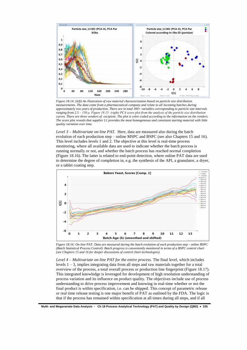
Figure 18.14: (left) An illustration of raw material characterization based on particle size distribution measurements. The data come from a pharmaceutical company and relate to all incoming batches during

approximately two years of production. There are in total 300+ variables corresponding to particle size intervals ranging from 2.5 – 150 μ. Figure 18.15: (right) PCA score plot from the analysis of the particle size distribution

curves. There are three vendors of excipient. The plot is color-coded according to the information on the vendors.

The score plot reveals that supplier L1 provides the most homogeneous and consistent starting material with little quality variation over time.

Level 3 – Multivariate on-line PAT. Here, data are measured also during the batch

evolution of each production step – online MSPC and BSPC (see also Chapters 15 and 16).

This level includes levels 1 and 2. The objective at this level is real-time process

monitoring, where all available data are used to indicate whether the batch process is

running normally or not, and whether the batch process has reached normal completion

(Figure 18.16). The latter is related to end-point detection, where online PAT data are used

to determine the degree of completion in, e.g. the synthesis of the API, a granulator, a dryer,

or a tablet coating step.

Figure 18.16: On-line PAT: Data are measured during the batch evolution of each production step - online BSPC (Batch Statistical Process Control). Batch progress is conveniently monitored in terms of a BSPC control chart

(see Chapters 15 and 16 for deeper discussions of control chart technologies).

Level 4 – Multivariate on-line PAT for the entire process. The final level, which includes

levels 1 – 3, implies integrating data from all steps and raw materials together for a total

overview of the process, a total overall process or production line fingerprint (Figure 18.17).

This integrated knowledge is leveraged for development of high resolution understanding of

process variation and its influence on product quality. The objectives include use of process

understanding to drive process improvement and knowing in real-time whether or not the

final product is within specification, i.e. can be shipped. This concept of parametric release

or real time release testing is one major benefit of PAT as outlined by the FDA. The logic is

that if the process has remained within specification at all times during all steps, and if all


raw materials were within specifications, then the final product must also be within

specification. This reasoning is of course based on the assumption that adequate data have

been measured on all parts of the process with sufficient frequency. This demands proper

and robust validation schemes and frequent monitoring of all measuring devices.

Figure 18.17: Overall on-line PAT: Combining information from all unit operations and raw materials for a

complete overview of the entire process. Involves levels 1-3.

18.5 A PAT example: Binary Powder II

18.5.1 Background to example and objectives

Diffuse reflectance NIR spectroscopy is a common method for analyzing powders. It is used

for both qualitative and quantitative analysis of powder mixing processes within the

pharmaceutical industry. A complicating feature of such studies is that a powder mixture

may be homogeneous with respect to its light absorption properties but not with regard to

light scattering.

In diffuse reflectance NIR, the spectrum of a powder sample is affected by both the

concentration of the excipients and the physical properties of the powder. The measured

reflectance is a combination of absorption, refraction and scattering of the incident light.

Light scattering properties are influenced by (i) particle size and shape, (ii) powder

distribution and packaging, and (iii) chemical composition of the powder.

The current example deals with mixing of two powders with dissimilar particle size, a fine

powder with particle size less than 200 μm and a coarse powder with particle size larger

than 300 μm. Such a marked difference in particle size may make the system susceptible to

segregation and hence real-time monitoring of the mixing process is particularly relevant.

Access to this dataset was kindly granted by Dr Ola Berntsson of AstraZeneca, Södertälje

[Berntsson, et al., 2000; Berntsson, 2001].

The objectives of the investigation are:

(i) to build a multivariate calibration model for predicting % coarse powder

(ii) to apply the calibration model for PSV of the powder blending process

(iii) to know when mixing is complete.

The example illustrates how PAT can be applied to an important unit operation in

pharmaceutical manufacturing.

18.5.2 Primary dataset

The primary dataset consists of 11 batches of powders, prepared and analyzed off-line, with

a coarse powder range of 0-100%. The 11 samples were prepared in separate bottles and

mixing was achieved by tumbling the bottles. After mixing, NIR spectra were acquired from

100 sub-samples of the powder in each bottle. The bottles were remixed between each

spectrum so that all 100 spectra collected represent different aliquots of the same powder

Dis-pensing

Granu-lation

Drying Milling Mixing Tabletting CoatingRawmaterial

NIR for QADoE in NIRfor selection

DoE and mixturedesign for recipe

NIR for w atercontent

Doe for setupPCA on particle

size curves

NIR forhomogeneity

DoE, PCA, PLSControlled Release

Curves

DoEDoE for time, w ater

Acoustics for stop

PAT for entire process

Process model

Model Model Model Model Model Model Model Model


sample. The spectra were obtained as log (1/R) in the 1080-2025 nm (9242 – 4937 cm-1)

range, using a nominal resolution of 32 cm-1, giving a total of 280 X-variables and 11*100 =

1100 observations.

The primary dataset was split into two parts, one for model training and the second for

model testing. All observations with 0, 20, 40, 60, 80 and 100% coarse powder (600

observations) constitute the training set while the test set is made up of the 10, 30, 50, 70

and 90% samples (500 observations).

18.5.3 Monitoring dataset

A vertical cone mixer was used which is appropriate for materials that are liable to

segregation (Figure 18.18). An orbiting transport screw creates a convection mixing

mechanism. NIR spectra were acquired by inserting a fiber-optic probe through an interface

in the cone wall. In the monitoring experiment, equal amounts of the coarse and fine

powders were loaded with the coarse powder on top. A total of 6000 spectra were monitored

with approximately 140 spectra corresponding to a single turn of the rotating convective

screw.

Figure 18.18: Schematic overview of the vertical cone mixer and the fiber-optic probe set-up.


18.5.4 Evaluation of raw data

From an examination of the raw spectra (Figure 18.19), both additive and multiplicative

effects are apparent. The higher the percentage of coarse powder the higher the spectral

pseudo-absorbances.

Figure 18.19: The 1100 spectra of the primary dataset.

For interpretation purposes, it is worth looking at the corresponding spectra of the pure

mixture components (Figure 18.20). The plot below shows the spectra of the pure powders

plus their difference (coarse-fine) spectrum. The pseudo-absorbances are higher for the

coarse powder.

Figure 18.20: Spectra for the ”pure” components and the difference spectrum coarse-fine.

18.5.5 PCA for data overview

It is good practice to get an overview of the spectral data using PCA. Relevant questions

include: Does the dataset contain groups? Are there any outliers? Is it appropriate to fit a

single calibration model or are separate models required? PCA can be performed sample-

wise, i.e. for 100 spectra at a time, or across the whole dataset, i.e. looking at all 1100

spectra in one global model. Fitting local models makes it easier to detect outliers and time

trends. On the other hand, the global model permits a comparison of the eleven samples, to

see whether there are time trends, jumps, discontinuities or other undesirable qualities in the

data.


We start by computing local PCA models of the 100 spectra of the sample containing 0%

coarse powder, 10% coarse powder and so on. Figure 18.21 shows representative results for

three out of the eleven possible local PCA models. All spectra were centered but not scaled

so the first principal component in each local model should be dominant. Indeed, the first

PC accounts for more than 97% of the variance in all eleven local models. Hence, it is

sufficient to focus only on t1. Figure 18.21 exemplifies how outliers can be detected using

line plots of t1. All sample models contain some spectral outliers.

Figure 18.21: Score line plots of t1 of three sample-wise PCA models, i.e., models for 20%, 50% and 80% coarse

powder samples. In each plot the vertical axis corresponds to the score values and the horizontal axis to the number order of the sub-sample spectra.

In the next phase, a global PCA model was fitted to all 1100 spectra to overview the entire

dataset and to investigate further the outliers observed previously during the local modeling

phase. Two principal components explain 99.9% of the original variation. Note that the first

component is far more important (95%) than the second. This needs to be borne in mind

when inspecting the score plot shown below (i.e. the horizontal direction is the dominant

spectral feature of Figure 18.22).

Figure 18.22: Score plot t1/t2 showing an overview of the 1100 observations (sub-sample spectra) contained in the

primary dataset. The plot is colored according to % coarse powder.

Figure 18.22 highlights a number of outliers, which are far from the other sub-samples in

the various batches and hence need to be removed. Most of these were also detected in the

local PCA models. We removed the following 29 observations: 69, 152, 191, 251, 261, 293,

312, 366, 372, 392, 440, 441, 469, 564, 572, 657, 663, 676, 685, 776, 788, 829, 854, 868,

877, 921, 934, 949 and 1098. After removing the outliers, the PCA model was refitted.

Again, the first component dominates and explains more than 95% of the spectral variation.

In the score plot below (Figure 18.23) there is a clear separation according to % coarse

powder. The plot suggests a boomerang shaped structure to the dataset, i.e. a non-linear

pattern. Samples with the highest amount of coarse powder are located to the right in the

score plot while the second component contrasts low percentage with medium-high

percentage coarse powder samples.

There are no new outliers. However, due to the large influence of the samples from the

100% batch, it might become necessary to exclude these observations during the calibration

phase to achieve a more balanced soft sensor model.


Figure 18.23: Score plot t1/t2 of the updated PCA model showing the separation among the various batches depending on the percentage coarse powder. The plot is colored according to % coarse powder.

The loading spectra shown below (Figure 18.24) confirm this interpretation. The first

component models baseline differences (recall that high percentage batches have higher

baseline offsets). The second component resembles the difference spectrum (coarse powder

– fine powder).

Figure 18.24: Line plot of the loading spectra of the first two principal components.

18.5.6 PLS model based on the training set

A PLS model with 10 components was fitted to the training set (containing 584 – not 600 –

observations following outlier removal). The X-scores of the first two components are

plotted in Figure 18.25. The grouped and curved pattern observed previously (cf Figure

18.23) is preserved. The strong non-linear structure is clearly seen in the t1/u1 score plot

shown in Figure 18.26.

This non-linearity can be explained by the large difference in scattering properties between

the two powders due to their differential particle sizes. One way to try to reduce the degree

of non-linearity is to log-transform the spectral data. This was tried but the results did not

change appreciably and the non-linear behavior was still apparent. Hence, in the following,

we will focus on the untransformed spectral data. Another option would be to eliminate the

samples from the 100% batch as these contribute most to the observed non-linearity.


Figure 18.25: (left) PLS X-score plot (t1/t2). The plot shows the relationship among the 584 spectra used to

calibrate the PLS model. Figure 18.26: (right) PLS X/Y score plot (t1/u1) suggesting a strong curvature to the

structure between X (NIR data) and Y (% coarse powder).

The loading spectra of the first three components are shown below (Figure 18.27). The first

component is related to the high percentage batches and therefore resembles the pure

spectrum of the coarse powder. The second loading spectrum mimics the difference

spectrum (coarse powder – fine powder). The third loading spectrum is hard to ascribe to

any specific chemical or physical phenomenon but captures information in the vicinity of

the peaks at 1200 and 1500 nm.

Figure 18.27: Line plot of the PLS loading weights (w*) of the first three components.

Subsequently, the calibration model was applied to the test set (containing 487 – not 500 –

observations following outlier removal). It can be seen from the t1/t2 plot (Figure 18.28) that

the training set is representative of the prediction set. Figure 18.29 displays the agreement

between observed and predicted Y-values.


Figure 18.28: (left) Projection of the test set observations onto the t1/t2 plane defined by the training set. The

training set is representative of the prediction set. Figure 18.29: (right) Relationship between observed and

predicted % coarse powder for the test set samples.

In summary, according to the observed vs. predicted plot, the relationship after 10

components is practically linear. Hence, the developed linear PLS model is able to cope

with the non-linearity, again demonstrating that the training set is representative of the test

set. The RMSEP is relatively low (≈ 4.3 %).

Due to the good predictive power on the test set it was deemed appropriate to apply the

multivariate calibration model to the monitoring dataset (see next section).

18.5.7 Application to the monitoring dataset

The next step consists of applying the calibration model to the monitoring dataset. However,

prior to that it is worth examining the raw spectra (Figure 18.30). Overall, these spectra look

similar to those acquired previously during the modeling phase. The two main differences

are that (i) the pseudo-absorbances are generally lower and (ii) the broad peak between 1400

and 1650 nm is more pronounced in the blending measurements.

Figure 18.30: The 6000 spectra contained in the monitoring dataset.

A more powerful way of comparing the spectra from the different data sources is by means

of the predicted score plot seen in Figure 18.31. The observations from the monitoring

dataset are quite different to those from the training set. They are also above Dcrit in the

DModX plots across all components (no plots provided). The unavoidable conclusion

therefore is that, because the monitoring spectra are too different from the training set, we

cannot expect the monitoring task to be of great practical value.


Figure 18.31: Predicted score plot. The monitoring spectra (shown in green) are situated differently compared

with the training and test set spectra (show in blue). Hence, we must realize that the calibration model is unrepresentative of the monitoring dataset.

The line plot of the predicted % coarse powder in the mixing process shows great variability

at the beginning of the campaign but rapidly stabilizes to a level of about 37-38% (Figure

18.32). The large variation at the beginning is due to the initial complete segregation of the

two powders. For each cycle of the orbiting screw the mixing is improved. The line plot

contains several spikes, which arise when the rotating equipment passes in front of the

probe window. In principle, a spike should be seen every 140th spectrum, however, due to

plot resolution restrictions not all spikes are seen. The magnifier functionality in the

software provides a better view of when the spikes occur. An alternative would be to create

a control chart of the “X-bar s” type using a sub-group size adjusted to the number of scans

per cycle of the orbiting screw. This will create a smoother trend curve. Such a plot is

illustrated in Section 18.5.10.

Figure 18.32: Line plot of the predicted % coarse powder.

It can be seen that powder homogeneity is reached about 30-40% into the mixing process

(between Num = 1800 to 2400), which is in agreement with the findings reported by the

original investigators. However, the predicted level of % coarse powder of 37-38% is not

satisfactory. The reason for this deviation from the nominal content of 50% is probably the

fact that the training data are not fully representative of the mixing data (recall the mismatch

detected in Figure 18.31), at least when working with uncorrected spectral data.


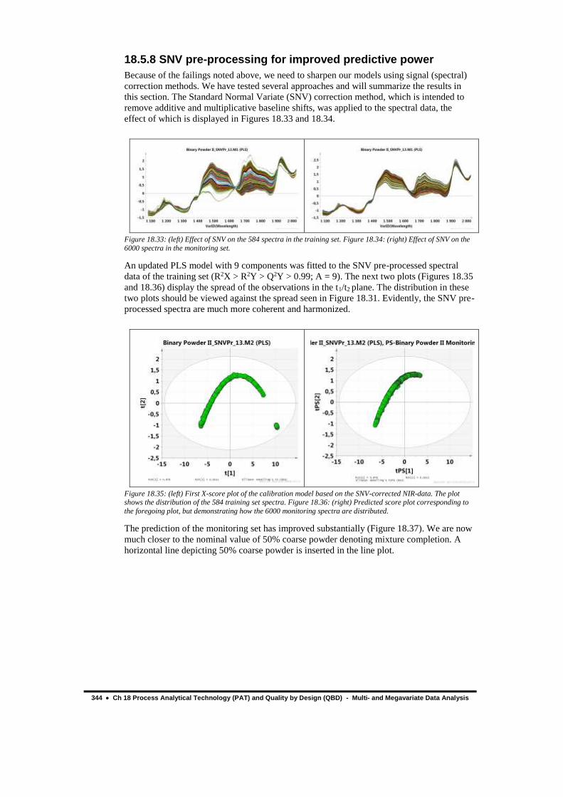
18.5.8 SNV pre-processing for improved predictive power

Because of the failings noted above, we need to sharpen our models using signal (spectral)

correction methods. We have tested several approaches and will summarize the results in

this section. The Standard Normal Variate (SNV) correction method, which is intended to

remove additive and multiplicative baseline shifts, was applied to the spectral data, the

effect of which is displayed in Figures 18.33 and 18.34.

Figure 18.33: (left) Effect of SNV on the 584 spectra in the training set. Figure 18.34: (right) Effect of SNV on the

6000 spectra in the monitoring set.

An updated PLS model with 9 components was fitted to the SNV pre-processed spectral

data of the training set (R2X > R2Y > Q2Y > 0.99; A = 9). The next two plots (Figures 18.35

and 18.36) display the spread of the observations in the t1/t2 plane. The distribution in these

two plots should be viewed against the spread seen in Figure 18.31. Evidently, the SNV pre-

processed spectra are much more coherent and harmonized.

Figure 18.35: (left) First X-score plot of the calibration model based on the SNV-corrected NIR-data. The plot shows the distribution of the 584 training set spectra. Figure 18.36: (right) Predicted score plot corresponding to

the foregoing plot, but demonstrating how the 6000 monitoring spectra are distributed.

The prediction of the monitoring set has improved substantially (Figure 18.37). We are now

much closer to the nominal value of 50% coarse powder denoting mixture completion. A

horizontal line depicting 50% coarse powder is inserted in the line plot.


Figure 18.37: Line plot of predicted % coarse powder for the monitoring data set. The plot suggests that a homogeneous mixture is achieved after 30-40 % of the time equivalents.

18.5.9 OPLS for enhanced interpretability

As discussed in Chapter 5, OPLS can be used to re-express a multivariate calibration model

in terms of components orthogonal to Y and components correlated to Y. We applied OPLS

to the SNV corrected spectral data. This produced an OPLS model consisting of nine

components, one predictive and eight orthogonal-in-X. The modeling statistics are displayed

in Figure 18.38. OPLS finds that 89% of the spectral variation is relevant for predicting the

% of coarse powder.

Figure 18.38: Summary of fit table for the OPLS model fitted to the SNV corrected data.

One way of comparing the PLS and OPLS models consists of comparing the scaled and

centered PLS regression coefficients with the Y-related profile of OPLS. Recall that the

basics of the Y-related profile coefficients were discussed in Section 5.4.4. The PLS

regression coefficients after nine components are plotted as a line plot in Figure 18.39 and

the corresponding OPLS Y-related profile is rendered in Figure 18.40. The OPLS Y-related

profile is much smoother and much more suggestive of real spectral features.


Figure 18.39: (left) PLS regression coefficients after nine components. Figure 18.40: (right) OPLS Y-related

profile.

Figure 18.41 provides additional information on the pure “constituents” (powders), which is

helpful when interpreting the meaning of the OPLS Y-related profile. Figure 18.41 shows

SNV-corrected pure spectra for the fine and coarse powders plus the difference spectrum

between them. The OPLS Y-related profile is plotted in the same plot. Note that all profiles

are scaled to fit in the same plot. There is a striking similarity between the OPLS Y-related

profile and the difference spectrum, particularly at the high-wavelength region end of the

spectral window.

Figure 18.41: Plot of SNV-corrected pure constituent spectra and the OPLS Y-related profile coefficients. Note

that all spectra are scaled to fit well in the same plot. The blue line represents the fine powder, the black line the coarse powder, the red line the difference, and the green line the Y-related profile coefficients. There is a striking

similarity between the Y-related profile and the difference spectrum.

With OPLS it is easy to visualize the effect of the division into predictive and orthogonal

components. The two inner relation (t1/u1) score plots in Figures 18.42 and 18.43 reveal that

OPLS removes a non-linear structure from the t/u relation.


Figure 18.42: (left) PLS t1/u1 score plot of the model based on SNV-corrected spectral data. This plot is

comparable to Figure 18.26. Figure 18.43: (right) OPLS t1/u1 score plot of the model based on SNV-corrected

spectral data. This plot is comparable to Figure 18.26.

Another interesting aspect of the OPLS model is that it allows the monitoring data to be

plotted as a single control chart of predicted t1 (Figure 18.44). When inspecting Figure

18.44 it should be noted that the average predicted t1 score for the 100 test set spectra with

50% coarse powder is -0.29. Hence, we again see that homogeneous mixing occurs within

30-40% of the sampling period.

Figure 18.44: Control chart of predicted OPLS t1-score values of the mixing process.

18.5.10 Discussion of example

This example clearly demonstrates that NIR is an appropriate instrumental technique for

modeling the relative amounts of the two powders. This indicates the suitability of

NIR/PLS/OPLS in pharmaceutical production unit operations, such as mixing and blending,

relevant in PAT.

Berntsson et al. have developed a simplified methodology for binary powders, based on

using relatively few calibration samples prepared and analyzed off-line [Berntsson, et al.,

2000; Berntsson, 2001]. The traditional approach to calibration is to collect one spectrum

from each of a number of calibration samples with known concentrations. However, when

heterogeneous powder samples are analyzed with reflectance spectroscopy, it is not possible

to assign a “true” concentration value to each spectrum. Instead, several spectra must be

acquired from different sub-fractions of each sample. The mean of these spectra is then used

in the calibration process to represent the nominal content of the sample.


From the results seen above, there is no doubt whatsoever that the methodology developed

by Berntsson et al. enables quantitative in situ monitoring of mixing processes using NIR.

NIR captures information about the mixture homogeneity in real time. The authors advocate

a high rate of in-line sampling (spectral acquisition) to get a detailed characterization of the

variation within the mixture. This method represents a useful tool for examining the

influence of various process parameters on the mixing time and mixing quality during the

development and scale-up of the process.

In a monitoring situation it is of interest to evaluate critical parameters as a function of time.

This is commonly done in multivariate statistical process control (MSPC). Within MSPC,

one may chart multivariate parameters, such as scores, Hotelling’s T2, DModX, predicted Y,

etc., using the conventional SPC control chart framework (Shewhart, EWMA & CuSum).

As an example, the plot below (Figure 18.45) provides a Shewhart chart of the predicted

level of % coarse powder in the mixing process monitored in-line and over time. The

process operator can easily follow, in real-time, how the mixing process evolves. To

facilitate interpretation, the progress of the mixing process is compared with the target value

and upper and lower warning and control limits (here corresponding to 2 and 3 standard

deviations).

Figure 18.45: Shewhart chart of predicted % coarse powder in the mixing process.

The plot above reveals that the mixing process is complete and stable from around 30-40%

into the sampling period. The spikes, which are due to the rotating screw passing in front of

the probe window, are clearly seen. One way to get rid of these spikes is to use sub-

grouping and co-chart the average Y-predicted value and the surrounding standard deviation

inside each sub-group. Such a control chart is shown below (Figure 18.46). When

constructing this plot, we used a sub-group size of 14, which means that 10 units on the

horizontal scale correspond to one complete turn of the orbiting screw.

The effect of the sub-grouping is a smoothed version of the Y-predicted trend curve. The

spikes are now evident in the standard deviation control chart as there is a peak at every

10th point (6, 16, 26, 36, etc.) in the control chart. Alternatively, one may choose to use a

larger sub-group size (say 140), but with larger size numbers there is a risk that the inherent

information and variation is partially “erased” from the control chart.


Figure 18.46: Tiled Shewhart charts of average Y-predicted value and the surrounding standard deviation inside

each sub-group.

In summary, in the current application, spectral pre-processing is necessary to get a working

in-line monitoring model. The combination of SNV and OPLS seems to be particularly

powerful. In this study, the external RMSEP is approximately 4.3%. The uncontrolled

experimental variation, generated by holding the fiber-optic probe against the powder

surface in 100 randomly chosen positions, may inflate the overall RMSEP. By comparing

the average predicted percentage coarse powder across the 100 observations of a powder

batch with the nominal content, it is estimated that roughly 50% of the overall RMSEP is

due to this instrumentation variability.

Thus, we strongly believe the calibration model obtained is useful for in-line monitoring of

the mixing process. We note that such a use of mixing process monitoring during routine

production is in line with the paradigm of real time parametric release, which focuses on

continuous quality assurance and improvements during all production steps, rather than

solely on the final step and final product.

18.6 Combining the concepts: The Novartis PAT example

18.6.1 Background

The last dataset to illustrate some of the concepts described in this chapter comes from a

feasibility study made together with Novartis in Suffern, NY, USA. We are grateful to

James Cheney, John Sheehan, and Fritz Erni for granting us permission to show this

example.

In this pharmaceutical production process, the manufactured tablets showed an unacceptable

tendency to dissolve too rapidly (dissolution rate less than 90). Process variables and

descriptions of the raw materials going into the tablets were available for a period of just

over two years. In the present investigation, only process data related to the dryer were


included because the operation of the dryer was suspected of causing the product quality

problems.

The process data comprise Ntot = 5743 observations with 6 process variables (e.g.

temperature, air flow, etc.) + process time for each. These observations are divided into Nbat

= 313 batches, which in turn are divided into 2 phases (steps). In addition, data for seven

raw materials (excipients) are available for each batch, as well as summary data for other

process steps (granulation, solvent addition, film coating), giving 298 variables in total.

Finally, 21 quality measurements are available for each batch, where the dissolution rate is

the most important.

Note that these data reside in different databases and are unaligned and unsynchronized so a

key part of the data analysis is to ensure that the batches are comparable and that the right

raw material data are aligned with the right batch.

18.6.2 Workflow to synchronize data

In this case, the data have different dimensions and sizes and it is therefore necessary to

align them to put them on a comparable footing. Getting the different types of data into a

single data structure was made according to the principles of hierarchical and batch-wise

analysis of process data outlined in [Wold, et al., 1996; Wold, et al., 1998b], see also

Chapters 16 and 19. Figure 18.47 shows an overview of the models’ structure.

Step 1. First, the data of the two phases were arranged in accordance with Figure

16.6. Two separate PLS models were made, one for each phase (step) of the

process using local process time as y (Figure 16.6).

Step 2. Subsequently, the original process variables were chopped up in one piece

per batch, transposed, aligned by linear time warping, and used as descriptors of

the process dynamics. The resulting matrix with one line per batch was then

subjected to a PLS analysis with y = dissolution rate. This gave 2 lower level

models (Figure 18.47).

Step 3. The data for each raw material (one row per batch) were fitted in separate

PLS models with y = dissolution rate. This gave an additional 7 lower level models

(Figure 18.47).

Step 4. The scores resulting from the 9 lower level PLS models developed in steps

2 and 3, in total 36 score variables, were used as variables in the “top hierarchical”

batch model, again with y = dissolution rate (Figure 18.47).

Figure 18.47: Overview of the modeling workflow to get a synchronized data structure. The structure seen is a

combination of batch analysis and hierarchical modeling. Each row is one batch.

The result of these three steps was that all the data were combined into a single, consistent

and synchronized structure. This allows the PLS estimation of the relationship between y =

dissolution rate and X = all data from the process, including raw materials, summarized

steps, and the full dynamics of the dryer.


18.6.3 Nine base level batch models

The PLS analysis was, as described in Section 18.6.2 above, divided into two hierarchical

levels. At the base level, 9 separate PLS models were built, each with the same y-variable

(dissolution rate), while the X-variables were from the two process steps and the 7 raw

materials. These 9 base models resulted in between 3 and 6 components each and a total of

36 score vectors. The models had R2X values of between 0.62 and 0.93 with an average of

0.72. The average R2Y was 0.15.

18.6.4 Top level batch model

The 36 base level score vectors were then used as X-variables (UV-scaled) in the top level

hierarchical PLS model. A two-component PLS model had R2X = 0.25, R2Y = 0.44 and

Q2Y = 0.39. The X-scores are plotted in Figure 18.48 and the relationship between observed

and predicted dissolution rate is shown in Figure 18.49. The score plot clearly contains

clusters and, by coloring by time, it becomes evident that later batches with poor dissolution

properties are clustered to the left (negative end of t1).

Figure 18.48: (left) Score scatter plot of t1/t2. A high proportion of late batches with poor dissolution properties are clustered in the left-hand region of the plot. Figure 18.49: (right) Agreement between measured and predicted

dissolution rate for the training set.

The model was validated by a permutation test (Figure 18.50), and by a final model

including more complete process data and its real on-line predictions (Figure 18.51).

Figure 18.50: (left) Validation plot based on 999 permutations of the y-vector followed by the fitting of a PLS

model between X (unperturbed) and the permuted y. The horizontal axis shows the correlation between the original and the permuted y, and the vertical axis the values of R2 (upper line, green) and Q2 (lower line, blue). The plot

where all Q2 values of the permuted y models are below zero is a clear indication that the original model does not

happen by coincidence. Figure 18.51: (right) Observed y = dissolution rate on the vertical axis plotted versus the predicted y from the top hierarchical PLS model later developed from more complete process data. Large points

are predictions for new batches. R2 = 0.82.


The top model PLS weights of the two components are plotted in Figure 18.52. Several raw

materials as well as one phase of the dryer are indicated as important for the changes in y =

dissolution rate. Further interpretation is available in [Wold and Kettaneh, 2005].

Figure 18.52: PLS-weights (w) for the first (horizontal axis) and second components (vertical axis) of the hierarchical top level PLS model.

18.6.5 Discussion and Epilogue

This hierarchical PLS modeling / process data mining exercise indicated that the process

quality variation could be explained. This led to the start of a much larger project looking at

all relevant data for both off-line modeling and on-line monitoring.

About a year after the first feasibility study, a system collecting, integrating, aligning, and

synchronizing all process and raw material measurements was in place at Novartis, Suffern.

A final PLS model was developed from all these data giving a remarkably good (and

validated) relationship with dissolution rate (Figure 18.51). This model was put on-line and

faithfully predicted dissolution rate for several months (large points in Figure 18.51). This is

a remarkable example and demonstrates how good models can be obtained, even when

dealing with extremely complex processes, provided that relevant data are available from all

parts of the process and that these data are properly aligned.

18.7 Questions for Chapter 18 1. What is PAT?

2. Which are the different levels of PAT?

3. What are their objectives?

4. What is QBD

5. What is a design space?

18.8 Summary and discussion The PAT concept encompasses a wide range of analytical technologies for in-line, on-line

or at-line measurements of pharmaceutical manufacturing processes with the basic objective

to determine whether the process and its intermediates and final product are “within

specifications”. A successful PAT implementation is characterized by a smooth integration

of process data sources (MES, ERP, LIMS, etc.) and instrumentation with computers and

pertinent software for data acquisition, data reduction, data analysis, storage of data and


results in databases, and presentation of results including the basis for the final batch record,

and when warranted, alarms and diagnostics indicating causes of problems and their

severity.

The implementation of PAT in a given process is not automatic and is not achieved

overnight. However, with a correct investment in adequate analytical measuring equipment,

computer networks, databases, chemometrics and other software, and training of personnel,

the return on these investments can be both large and immediate. Waiting time between

sampling and analytical results are dramatically reduced or even eliminated, the reliability

of results improved, scrap reduced, and process understanding improved.

As mentioned in Section 18.4.4, real time release testing (RTRT) is a major benefit of PAT.

To accomplish RTRT, the vast array of model types discussed in this book can be used.

These models include multivariate calibration models, surrogate models, design space

models and MSPC models. A surrogate model is a multivariate model based on fast process

measurements that is replacing traditional and time-consuming measurements. When used

in conjunction, such models ultimately provide a higher assurance of product quality.

To quote the ICH Q8 (R2) guidance document, RTRT represents “the ability to evaluate and

ensure the quality of in-process and/or final product based on process data”. Interestingly, in

a presentation at the AAPS Annual Meeting, Washington, October 2011, the acting director

of FDA, C.M.V. Moore, discusses a regulatory perspective on RTRT. According to this

perspective, RTRT brings about a number of benefits, including (i) increased assurance of

quality, (ii) increased manufacturing flexibility and efficiency and (iii) enhanced process

understanding. Furthermore, an account is given as to how RTRT relates to QBD. There is

no one-to-one relationship between QBD and RTRT, however, as stated by C.M.V. Moore

“it would be difficult to justify RTRT without a science and risk based approach”.

The obvious extension to using multivariate models and design space models for monitoring

and prediction is model predictive control (MPC) of processes [Lauri, et al., 2010;

McCready, 2011; Tian, et al., 2011]. Below, we briefly describe an approach to multivariate

batch control denoted SIMCA-control, which is based on the work of McCready

[McCready, C., 2011]. SIMCA-control is a model predictive control (MPC) method

integrated within the multivariate modeling techniques in Umetrics’ SIMCA software

family (SIMCA-online and SIMCA).

There are two forms of batch control included in SIMCA-control, batch evolution control

(BEC) and batch level control (BLC). The objective of BEC is to find the set of manipulated

variables (XMV) and their settings that maintain the batch process on a defined batch

evolution trajectory (see example in Figure 18.53). An example may include the adjustment

of nutrient flows so that a batch evolution model score value is maintained within SPC

limits. It is envisioned that BEC is a regulatory type of control executed at a relatively high

frequency.


Figure 18.53: The figure depicts an example batch evolution control chart containing the information presently provided in SIMCA-online, including the measured process up to the current maturity (black), the model average

(green) and +/- 3 control limits (red). With SIMCA-control these control charts may also include the desired

trajectory (green dashed) as well as open loop (red dashed) and closed loop (blue dashed) predicted trajectories. Open loop refers to the predicted trajectory of the process if no process adjustments are implemented. Closed loop

refers to the predicted trajectory of the process if the adjustments from SIMCA-control are implemented.

For batch level control (BLC) the goal is to find the set of XMV and their settings that result

in optimized final batch conditions. An example may include adjustment of nutrient levels

to maximize the yield at the end of fermentation. It is envisioned that BLC is a supervisory

type of control that is only executed at selected times for mid-course type correction. A

schematic batch evolution control chart is shown in Figure 18.54.

These two methods, BEC and BLC, may be paired up in a cascade configuration to provide

both regulatory (frequent adjustments to keep the process in-control) and supervisory (mid

course correction) control of final qualities.

Figure 18.54: Batch level control chart showing predicted open and closed loop final batch performance.


The SIMCA-online software is used in many industries for monitoring of batch systems. It

executes SIMCA offline model files. With the predictive capabilities of SIMCA-control,

monitoring is enhanced by providing reliable predictions of future process performance.

Model predictive control (MPC) is a technique where adjustments to a process are selected

by finding the set of manipulated variables (XMV) and their settings that result in an optimal

process performance. Traditionally only process outputs (Y) are considered in the objective

function. With SIMCA-control, multivariate terms are integrated into the objective function

to assure that the adjustments made by the controller are constrained to the knowledge space

[McCready, 2011]. This is especially important for regulated industries, such as

pharmaceutical and biopharmaceutical, where a process must be shown to operate within

regions that assure good quality product (the design space).

Documents

Process Analytical Technology (PAT) and Quality by Design (QbD)