IEEE HUNGARY SECTION

PROCEEDINGSOF THE

11TH PHD MINI-SYMPOSIUM

FEBRUARY 3–4, 2004.

BUDAPEST UNIVERSITY OF TECHNOLOGY AND ECONOMICS

DEPARTMENT OF MEASUREMENT AND INFORMATION SYSTEMS

PROCEEDINGSOF THE

11TH PHD MINI-SYMPOSIUM

FEBRUARY 3–4, 2004.BUDAPEST UNIVERSITY OF TECHNOLOGY AND ECONOMICS

BUILDING I, GROUND FLOOR 017.

BUDAPEST UNIVERSITY OF TECHNOLOGY AND ECONOMICS

DEPARTMENT OF MEASUREMENT AND INFORMATION SYSTEMS

2004 by the Department of Measurement and Information Systems Head of the Department: Prof. Dr. Gábor Péceli

Conference Chairman: Béla Pataki

Organizers:

Nóra Székely Csaba Dezsényi

Gergely Tóth Gergely Pintér

Homepage of the Conference:

http://www.mit.bme.hu/events/minisy2004/index.html

Sponsored by: IEEE Hungary Section (technical sponsorship)

Foundation for the Technological Progress of Industry – IMFA Allied Visions

ISBN 963 420 785 5

FOREWORD

This proceedings is a collection of the extended abstracts of the lectures of the 11th PhD Mini-Symposium held at the Department of Measurement and Information Systems of the Budapest University of Technology and Economics. The main purpose of these symposiums is to give an opportunity to the PhD students of our department to present a summary of their work done in the preceding year. Beyond this actual goal, it turned out that the proceedings of our symposiums give an interesting overview of the research and PhD education carried out in our department. The lectures reflect partly the scientific fields and work of the students, but we think that an insight into the research and development activity of the department is also given by these contributions. Traditionally our activity was focused on measurement and instrumentation. The area has slowly changed during the last few years. New areas mainly connected to embedded information systems, new aspects e.g. dependability and security are now in our scope of interest as well. Both theoretical and practical aspects are dealt with.

The papers of this proceedings are sorted into six main groups. These are Biomedical Engineering, Information Systems, Intelligent Systems, Modeling, Networking and Signal Processing. The lectures are at different levels: some of them present the very first results of a research, because some of the first year students have been working on their fields only for half a year. The second and third year students are more experienced and have more results.

During this eleven-year period there have been shorter or longer cooperation between our department and some international research institutes, some PhD research works gained a lot from these connections. In the last year the cooperation was especially fruitful with the Vrije Universiteit Brussel, University of Erlangen, Oregon State University, Pisa Dependable Computing Center, Nokia, IBM, Technische Universität Berlin and the SOFTSPEZ Project Consortium.

We hope that similarly to the previous years, also this PhD Mini-Symposium will be useful for both the lecturers and the audience.

Budapest, January 14, 2004. Béla Pataki Chairman of the PhD Mini-Symposium

LIST OF PARTICIPANTS

PARTICIPANT ADVISOR STARTING YEAR OF PHD COURSE

Zoltán BALATON Ferenc VAJDA .........................................................................2003 Károly János BRETZ Ákos JOBBÁGY ......................................................................2003 Csaba DEZSÉNYI Tadeusz DOBROWIECKI ........................................................2002 Péter DOMOKOS István MAJZIK.........................................................................2003 Csilla ENDRŐDI Endre SELÉNYI .......................................................................2001 László GÖNCZY Endre SELÉNYI .......................................................................2003 Szilvia GYAPAY András PATARICZA................................................................2001 András KOVÁCS Tadeusz DOBROWIECKI ........................................................2001 Dániel László KOVÁCS Tadeusz DOBROWIECKI ........................................................2003 László LASZTOVICZA Béla PATAKI ...........................................................................2003 János MÁRKUS István KOLLÁR .......................................................................2000 Károly MOLNÁR Gábor PÉCELI..........................................................................2003 Elemér Károly NAGY András SZEGI ..........................................................................2003 Gergely PINTÉR István MAJZIK.........................................................................2002 András RÖVID Annamária VÁRKONYI-KÓCZY ............................................2001 László SRAGNER Gábor HORVÁTH....................................................................2002 Péter SZÁNTÓ Béla FEHÉR .............................................................................2004 Dániel SZEGŐ Endre SELÉNYI .......................................................................2000 Nóra SZÉKELY Béla PATAKI ...........................................................................2002 Ákos SZŐKE András PATARICZA................................................................2003 Béla TOLVAJ István MAJZIK.........................................................................2001 Gergely TÓTH Ferenc VAJDA .........................................................................2002 Norbert TÓTH Béla PATAKI ...........................................................................2003 Péter VARGA Tadeusz DOBROWIECKI ........................................................2003

PROGRAM OF THE MINI-SYMPOSIUM

SIGNAL PROCESSING chairman: Gábor Péceli

János MÁRKUS Monotonicity of Digitally Calibrated Cyclic A/D Converters ........ 8 László SRAGNER Modeling of a Slightly Nonlinear System...................................... 10 András RÖVID Car Body Deformation Based on Soft Computing Techniques..... 12 Károly MOLNÁR Synchronization of Sampling in Intelligent Sensor Networks....... 14 Péter SZÁNTÓ 3D Rendering: Minimizing the Overhead of Non-Visible Pixels .. 16

INFORMATION SYSTEMS chairman: Tadeusz Dobrowiecki

Szilvia GYAPAY Solving the Optimal Trajectory Problem using SPIN ................... 18 Gergely PINTÉR Checkpoint and Recovery in Diverse Software............................. 20 Dániel SZEGŐ A Logical Methodology for Processing Web Documents ............. 22 Csaba DEZSÉNYI A Framework for Information Extraction ..................................... 24

INTELLIGENT SYSTEMS chairman: Gábor Horváth

András KOVÁCS A Dominance Framework for Constraint Programming .............. 26 Péter VARGA Information Extraction with Ontologies ....................................... 28 Dániel László KOVÁCS Towards Rational Agency ............................................................. 30

MODELING chairman: István Majzik

Elemér Károly NAGY Some Optimization Problems of Elevator Systems ....................... 32 Péter DOMOKOS From UML Class Diagrams to Timed Petri Nets ......................... 34 Ákos SZŐKE Quality Metrics and Models in Software Development Processes 36 Béla TOLVAJ Trace-Based Load Characterization using Data Mining ............. 38

NETWORKING chairman: Ferenc Vajda

Zoltán BALATON Grid Information and Monitoring Systems ................................... 40 László GÖNCZY Design of Robust Web Services..................................................... 42 Csilla ENDRŐDI RSA Timing Attack Based on Logical Execution Time ................. 44 Gergely TÓTH General-Purpose Secure Anonymity Architecture ........................ 46

BIOMEDICAL ENGINEERING chairman: Béla Pataki

Károly János BRETZ Objective Evaluation of the Tremor.............................................. 48 László LASZTOVICZA Microcalcification Detection using Neural Networks .................. 50 Norbert TÓTH Texture Analysis of Mammograms................................................ 52 Nóra SZÉKELY Tumor Detection on Preprocessed Mammograms........................ 54

CONFERENCE SCHEDULE

TIME FEBRUARY 3, 2004

TUESDAY TIME

FEBRUARY 4, 2004

WEDNESDAY

8:30 CONFERENCE OPENING

Opening speech: Gábor Péceli

8:40 SIGNAL PROCESSING 8:30 NETWORKING

10:50 INFORMATION SYSTEMS 10:20 BIOMEDICAL ENGINEERING

LUNCH BREAK

13:30 INTELLIGENT SYSTEMS

15:00 MODELING

MONOTONICITY OF DIGITALLY CALIBRATED CYCLIC A/DCONVERTERS

Janos MARKUSAdvisor: Istvan KOLLAR

I. Introduction

Analog-to-digital converter designers are always searching for new converter structures, which haveadvantageous properties compared to their predecessors (e.g. higher resolution, higher speed, or lowerpower consumption).

Cyclic converters, which form a special group

×g ΣS/H

+

−

Vin

Residue−

−Vref+Vref

di

(to serial register)

D/AA/D

Figure 1: Block diagram of a cyclic converter.Vin: input signal, Vref : reference signal, g: radixnumber (g = 2 in an ideal case), di: one-bitdigital output.

within the 1-bit/stage sub-ranging converters, areeasy to design, and they are good candidates toachieve very small power- and area consumption.Fig. 1 shows the block diagram of such a converter.Its operation is as follows. In the first cycle, theinput signal is sampled and quantized by a one-bitA/D, then the quantized signal is converted to ana-log again by the D/A and subtracted from the input,which is multiplied by the radix number g (g = 2in an ideal case). In the next cycle, this residue isused as an input signal to obtain the second MSB,and so on, up to n. The output of the converter (the

sequence of di) is the binary representation of the input signal in an ideal case.Due to analog component mismatches, the radix number g becomes inaccurate, and thus the resolu-

tion of these converters is limited to 10-12 bit using standard technologies. To enhance the resolution,digital self-calibration can be used [1, 2]. Note that if g is inaccurate, two types of error exist [1]. Ifg > 2, at specific inputs at least one stage will be saturated, causing missing-decision-level error (i.e.,the output does not change for a wide range of the input signal). If g < 2, missing codes will beintroduced in the output (i.e., the output jumps for a small change in the input signal). Note that digitalcalibration, which simply reassigns the digital codes to another ones, does not correct for the first typeof errors, thus a nominal g < 2 must be used in these converters, and more stages must be used tocompensate for the resolution loss [1, 2].

In the next section it is shown that all sub-ranging converters with g < 2 produce non-monotonicoutput. A method to avoid this behaviour is also suggested.

II. Monotonicity of the Converters

As noted in the previous section, in an ideal case, when g = 2, the di output sequence of the converteris the binary representation of the input signal. By using a nominal gain g < 2, however, the outputsequence becomes radix-g based, i.e., the output can be calculated as [2, 3]

D =

n−1∑

i=0

gid′i, (1)

where d′0 is the LSB and d′

n−1 is the MSB value of the digital word.

500 1000 1500 2000 2500 3000 3500 40000

500

1000

1500

2000

2500

3000

Input Code [binary]

Ou

tpu

t C

od

e [

g−b

ased

]

(a)

−1 −0.5 0 0.5 1−1

−0.8

−0.6

−0.4

−0.2

0

0.2

0.4

0.6

0.8

1(b)

Ou

tpu

t [V

/Vre

f]

Input [V/Vref

]164 165 166 167 168 169

163

164

165

166

167

168

169

170(c)

Ou

tpu

t [L

SB

10]

Input [LSB10

]

Figure 2: Different outputs of an n = 12-cycle, g = 1.95 cyclic converter. (a) All possible outputsof Eq. (1). (b) Real outputs of the converter. (c) 10-bit non-monotonic output example (dashed line:12-bit code, solid line: 10-bit requantized code).

Calculating all possible codes with Eq. (1) results in huge non-monotonic jumps in the output(Fig. 2(a)). In reality, as discussed in the introduction, a cyclic converter with g < 2 exhibits missingcodes. In addition, based on the converter’s operation, it can be shown [3] that the absolute differencebetween the input signal and its radix-based representation (Eq. (1)) is always less then or equal to oneLSB. Although this behaviour ensures that the difference between two consecutive digital outputs isless then or equal to one LSB, it allows this difference to be negative, thus, it allows non-monotonicbehaviour, if such difference exists. It can be shown [3] that for any g ∈ (1, 2) such code transition al-ways exists. For example, if g = 1.95, then code transition xxxx xx01 1111 → xxxx xx10 0000 causesa negative step of -0.431 LSB. Such an example is enlarged in the inset of Fig. 2(b).

As noted in the introduction, using g < 2 causes resolution loss, thus more stages must be used fora given resolution. In other words, the calculated output code (cf. Eq. (1)) must be requantized tonbit ≤ n − 2 bit [2]. Thus, the final LSB size will be 2–3 times larger then the step size of the radix-based converter, smoothing out most of the non-monotonic transitions. However, it can be shown [3]that there will always be some negative code transitions which crosses one of the (re)quantizationthresholds, causing non-monotonic behaviour even in the final output. Such an example is depicted inFig. 2(c).

In critical applications where this behaviour is not acceptable, it can be removed by a simple digitalalgorithm: in any cases where the 12-bit g = 1.95-based output code contains 5 consecutive ones,subtracting one LSB, and where it contains 5 consecutive zeros, adding 1 LSB removes all the non-monotonic transitions while still maintains the same resolution.

III. Conclusion

In this paper the non-monotonic property of digitally calibrated cyclic converters was introduced. Itwas shown that this behaviour always exists if the nominal gain (g) is less then two. A simple digitalalgorithm was suggested to ensure monotonicity. Both the theory and the solution can be extended toother 1-bit/stage sub-ranging converters with g ∈ (1, 2).

References

[1] A. N. Karanicolas, H.-S. Lee, and K. L. Bacrania, “A 15-b 1-Msample/s digitally self-calibrated pipeline ADC,” IEEEJournal of Solid-State Circuits, 28(12):1207–15, Dec. 1993.

[2] O. E. Erdogan, P. J. Hurst, and S. H. Lewis, “A 12-b digital-background-calibrated algorithmic ADC with -90-dBTHD,” IEEE Journal of Solid-State Circuits, 34(12):1812–20, Dec. 1999.

[3] J. Markus and I. Kollar, “On the monotonicity and maximum linearity of ideal radix-based A/D converters,” in IEEEInstrumentation and Measurement Technology Conference, IMTC’2004, Como, Italy, 18–20 May 2004, submitted forpublication.

MODELING OF A SLIGHTLY NONLINEAR SYSTEM László SRAGNER

Advisors: Gábor HORVÁTH, Johan SCHOUKENS

I. Introduction System identification is a process of deriving a mathematical model using the observed data.

Depending on the type of the system the difficulties of model building maybe rather different. The area of linear system modeling is well developed, but for the nonlinear case there are a lot of open problems. A special field is the modeling of slightly nonlinear systems. In these cases a rather good model can be constructed using the linear approach, however if a highly accurate model is required the nonlinearities of the system must be taken into consideration. For slightly nonlinear systems general nonlinear modeling approach – like neural networks – can be used or the starting point can be a linear model, which must be modified somehow. This paper presents some results of slightly nonlinear dynamic system modeling.

II. The Modeling with Neural Networks A classical neural network creates a static nonlinear mapping between the input and the output

data, therefore to make it applicable for dynamic real world problems it has to be extended. This can be easily done using the NARX model class which creates an open loop model from the measured data [1]: ( ) ( ) ( ) ( ) ( ) ( ) ( ) ( )[ ]mtdtdtdltutututut −−−−−−= ,..2,1,,..2,1,x (1) ( ) ( )( ) ( )( )∑

=

++==N

iii

TiiNN cbtvtfty

1tanh, xwxw (2)

Here u is the measured input, d is the measured output, (m,l) is the order of the model, ( ).NNf is the transfer function of the static neural network and w is the parameter vector. Usually the static neural network is realized by a Multi-Layer Perceptron. The direct use of this dynamic neural network often does not lead to good results because the training method may stuck in local minimum. To avoid this we create a special weight initialization method. With the same model order (m,l) we create the best linear approximation. We calculate the linw vector to minimize the value of the linear cost function:

( ) ( )( )∑=

−T

t

Tlin ttd

1

2*xw where T is the length of the time series. Then we replace every iw with linw plus a small random value, to make the outputs of the neurons slightly different. Every iv is set to 1/N where N is the number of the neurons. With this model structure and weight initialization we can create a nonlinear model starting from a good linear estimation of the problem. The training can be done by simple gradient descent method or the Levenberg-Marquardt training algorithm. The number of neurons depends on the complexity of the modeling system, but it has to be small enough to avoid overtraining.

III. Experimental Results The experiments are done on a nonlinear electrical circuit. It approximates a physical model

described by the following nonlinear second order differential equation: ( ) ( ) ( ) ( ) ( ) ( )tutyctyctyctydt

dbtydtda =++++ 3

32

212

2 (3)

The excitation signal is a normally distributed noise with slowly increasing standard deviation to observe the input dependent nonlinearities of the model.

IV. Difference Between Prediction and Simulation Error Prediction error is defined as:

( ) ( ) ( ) ( ) ( )( )tftdtytdte NNpredpred xw,−=−= (4) where x(t) is defined as in (1). Simulation error is defined as:

( ) ( ) ( ) ( ) ( )( )tftdtytdte NNsimsim xw ˆ,−=−= (5) where ( )tx is defined as:

( ) ( ) ( ) ( ) ( ) ( ) ( ) ( )[ ]mtytytyltutututut −−−−−−= ,..2,1,,..2,1,x (6) The model is created by minimizing the prediction error, because it is an open loop model and in

this case the training process is stable. With the simulation error we can observe the response of the model for unknown outputs. In this case we use a closed loop model so we have to take care of the stability problems. If our nonlinear model has large errors then the response of our model will be unstable.

Figure 1: Three graphs of the observed errors

V. Conclusion and Further Tasks The nonlinear model with our weight initialization captures the relevant nonlinear behaviour of the

system, especially at large standard deviations (the nonlinear behaviour here is stronger because the cubic term in (3)). The rare high peaks in simulation error is due to input points far from the center of the input domain (the mean of x(t)-s over t). To avoid this can be a task for further researches.

References [1] K. S. Narendra, K. Pathasarathy, “Identification and Control of Dynamical Systems Using Neural Networks”, IEEE

Trans. on Neural Networks, Vol.1.pp. 4-27,1990. [2] J. Schoukens, J. Nemeth, P. Crama, Y. Rolain, and R. Pintelon. “Fast approximate identification of nonlinear

systems”. SYSID 2003, Rotterdam pp. 61-66

CAR BODY DEFORMATION DETERMINATION BASED ON SOFT COMPUTING TECHNIQUES

András RÖVID Advisors: Annamária R. VÁRKONYI-KÓCZY, Gábor MELEGH

I. Introduction The energy absorbed by the deformed car body is one of the most important factors affecting the

accidents thus it plays a very important role in car crash tests and accident analysis [1]. There is an ever-increasing need for more correct techniques, which need less computational time and can more widely be used. Thus, new modeling and calculating methods are highly welcome in deformation analysis.

Intelligent computing methods (like fuzzy and neural network (NN) based techniques) are of great help in this. Based on them we can construct systems capable to determine the energy absorbed by the car-body deformation using only digital pictures as inputs.

The paper is organized as follows: In Section II. the determination of the absorbed energy will be discussed. Section III. will be devoted to the details of the digital photo based 3D modeling of the crashed car body, while Section IV will present the determination of the direction of the impact together with the amount of absorbed energy. Conclusion will be summarized in Section V.

II. Determination of the Deformation Energy from Digital Pictures The evaluation of the car-body deformation is done in two steps. First, the 3D shape of the

deformed car-body is created with the help of digital pictures taken from different camera positions. As the second step, the 3D car-body model is processed by an intelligent computing system. The system needs only the above-mentioned digital pictures as inputs, while as outputs; we get the direction of the impact and the deformation energy absorbed by the car-body elements. The processing time of this method is much less than the processing time of the past methods, i.e. it can supply the outputs already at the accident plotting time. This property is very advantageous in supporting the work of road accident experts.

III. Extraction of the 3D Car-Body Model from Digital Images To get the 3D model of the deformed car body and to limit/delimit the objects in the picture from

each other is of vital importance. As the first step, the pictures, used in the 3D object reconstruction are preprocessed. As a result of the preprocessing procedure the noise is eliminated. For this purpose we apply intelligent fuzzy filters [2]. After noise filtering, the edges – object boundaries – are detected with the help of a fuzzy based edge detector [3].

The preprocessing is followed by the determination of the 3D coordinates of the car-body edge points. To determine the 3D position of the image points it is necessary to have at least two images taken from different camera positions. We also have to determine the projection matrix for each image.

The last step before modeling is the determination of the corresponding pixels (points) in the analyzed images [4]. Methods of linear algebra and object recognition are used for this purpose. In view of these factors we can calculate the 3D position of the image points of the deformed car-body and so design the spatial model.

Figure 1: Block diagram of the system

IV. Determination of the Direction of the Impact and the Absorbed Energy After constructing the 3D model of the deformed-car body we have to determine the volume of the

deteriorated car body. This operation is performed by an individual module and as result; we obtain the volumetrical difference between the undamaged and damaged models. The direction of the impact will be determined by a further module based on fuzzy-neural networks also working with the model of the deformed car-body. From the volumetrical difference and from the direction of impact an intelligent computing system can evaluate the energy absorbed by the deformation and the equivalent energy equivalent speed (EES). During the teaching period of the system, the determined EES values are compared to the outputs of the real system and the parameters of the expert system are modified according to a suitable adaptation mechanism to minimize the error (see Figure 1). The latter parts of the global system mentioned here are designed but not yet implemented.

V. Future Work, Conclusions This paper introduces a new intelligent method for deformation’s energy determination, as well as

for the photo-based determination of the deformation’s spatial shape. Based on it, the block design of an intelligent expert system is presented which makes easy to determine the amount of the energy absorbed by the deformation and further important information, e.g. in car crash analysis the car-body deformation and the energy equivalent speed. As our future work, we will implement the missing, only theoretically designed parts of the system: an algorithm for the automatic determination of the corresponding pixels in the analyzed images to be able to build the 3D model without external interventions and a fuzzy-NN based system for the estimation of the spatial model of the deformed car-body to get the deformation’s energy (and the energy equivalent speed) and the direction of the impact.

References [1] A. Happer, M. Araszewski, Practical Analysis Technique for Quantifying Sideswipe Collisions, 1999. [2] F. Russo, “Fuzzy Filtering of Noisy Sensor Data”, in Proc. of the IEEE Instrumentation and Measurement

Technology Conference, pp. 1281-1285, Brussels, Belgium, 4-6 June 1996. [3] F. Russo, “Edge Detection in Noisy Images Using Fuzzy Reasoning”, IEEE Transactions on Instrumentation and

Measurement, Vol. 47, No. 5, Oct. 1998, pp. 1102-1105. [4] R. Koch, M. Pollefeys, and L. Van Gool. “Multi viewpoint stereo from uncalibrated video sequences”, in Proc. of

the 5th European Conference on Computer Vision, Vol. I, pp. 55–71, 1998.

SYNCHRONIZATION OF SAMPLING IN INTELLIGENT SENSORNETWORKS

Karoly MOLNARAdvisors: Gabor PECELI, Laszlo SUJBERT

I. Introduction

An intelligent sensor network is a distributed signal processing system, which consists of interactingnodes performing real-time data acquisition and signal processing. An overview of this system ispresented in Fig.1. A node is basically a low-scale processing unit (a DSP or a microprocessor thatperforms digital signal processing) that processes discrete data from sensors via AD converters. Theuse of these systems are more and more widespread, e.g. in seismic wave measurements.

The nodes are performing online signal pro-

Figure 1: System Architecture

cessing, i.e. the samples of the sensors arecontinuously processed. This operation is con-trolled by a clock signal, that triggers the sam-pling instant of the AD. These sampling clockshave to be synchronized in frequency in or-der to ensure the consistent operation of thenodes. The phase synchronization is also im-portant, as most applications need concurrentmeasurements of the same process. In order tosynchronize the nodes, the clock signals haveto be transmitted among them. Therefore, the communication medium of the sensor network highlyinfluences the implementation of the theoretic synchronization methods. Effects such as delay, jitterand signal loss have to be considered.

II. Network Synchronization Basics

In intelligent sensor networks the following network states are defined [1]: asynchronous, frequencysynchronous (FS) and phase synchronous (PS). The long-term frequency drift due to component agingis neglected, as this effect is presumed to be compensated together with the frequency synchronization.

From the point of view of synchronization, the following network topologies are defined: FullyConnected (FC), Partially Connected (PC) and Master-Slave (MS). In FC networks, a synchronizationsignal is transmitted from each node to every other node. In PC networks, there are no synchronizationconnection between some of the node pairs. In the MS case, a free-running master transmits its clocksignal to the slave nodes. In any case, each node synchronizes its own sampling clock to the receivedsignal(s) i.e. a phase-locked loop (PLL) structure has to be implemented.

III. Possible Solutions

A. DPLL Realized on DSP

As the nodes have a processing unit, there are several possibilities to implement the PLL structure. Inthis paper, the digital implementation (DPLL) possibilities are examined. This solution is advantageousas the whole signal processing is realized in DSP software, it is possible to develop specific algorithmsin order to compensate the various errors of the communication medium of the network.

The synchronization of the sampling clocks depends on the type of the AD converter used in thenode. The sigma-delta AD converters need an N-times greater clock frequency than the sampling rate,as the sigma-delta modulation is based on oversampling (N is typically 64..256). Flash and successive-approximation converters need a sampling clock equal to the sampling rate.

The master-clock is a theoretically periodic signal received via the communication medium. Practi-cally this signal is quasi-periodic from the point of view of the DSP, regardless of the specific realiza-tion. The output of the PLL is a logic signal to the clock pin of the AD.

A possible DPLL realization is shown in [2]. The DPLL structure is described by a differenceequation, that is analyzed in the Z-domain. The components of this structure are: phase detector, loopfilter, digital controlled oscillator and a frequency divider. This approach resembles the analog PLLstructure. Another possibility is to build a functional DPLL that provides an output signal synchronizedto the received clock signal. This algorithm can be featured to handle the transmission errors introducedby the network medium of the system.

B. DPLL Realization with DDS ICThe sampling clock is an output of the DSP, so it is synchronous to the system clock, therefore

the frequency of the sampling clock signal is discrete, and the resolution is equal to the CPU clockfrequency. In addition, the frequency of the CPU limits the maximum frequency of the output signal.In case of fast DSPs, and low sampling rates this effect can be neglected, but in some cases it is aserious issue, e.g. if sigma-delta AD converters are used. In this case, due to the need for high clockfrequencies for oversampling, it is impossible to use direct output from a DSP. When high frequenciesare needed, a specific DDS IC can be used [3] to provide the clock signal. These programmable ICsprovide precise high frequency signals by Direct Digital Synthesis. This is a promising solution, theoperation of a DDS IC controlled by a DSP is an interesting area of future research.

C. Software SynchronizationThe sampling synchronization can also be implemented in software. The AD converters of the nodes

are in a free-run state and the network is in asynchronous state. The solution is based on the conceptthat the synchronization of the signal processing nodes and the sampling has to be separated. TheDSP handles the following two asynchronous events: (i) new sample arrives from the AD (ti), (ii) tickof the master clock (tMaster). The DSP calculates the value of the analog signal at tMaster from theavailable f(ti) sample values by interpolation. In other words, the discrete signa l that is the outputof the AD is resampled with the frequency of the master clock. This solution is already implementedon a test-system, that comprises of two identical DSP nodes with asynchronous sigma-delta converters[4]. The interpolation calculation was realized three different ways: linear interpolation, interpolationfiltering and interpolation filtering combined with linear interpolation.

IV. Conclusion

In this paper, the problem of synchronization of sampling in intelligent sensor networks was con-sidered. The different DSP-based solution possibilities were examined, and a software solution wasimplemented on a test system. Subject of future research is the DPLL-based implementation.

References[1] J.-H. Chen and W. C. Lindsey, “Network frequency synchronization – part-i.,” MILCOM ‘98, Boston, Oct. 1998.[2] T. M. Almeida and M. S. Piedade, “DPLL design and realization on a DSP,” in Proc. of the ICSPAT International

Conference on Signal Processing Applications and Technology, San Diego, USA, 1997.[3] Analog Devices, A Technical Tutorial on Digital Signal Synthesis, Analog Devices, Inc., 1999.[4] K. Molnar, L. Sujbert, and G. Peceli, “Synchronization of sampling in distributed signal processing systems,” in Proc.

of the 2003 IEEE International Symposium on Intelligent Signal Processing, pp. 21–26, Budapest, Hungary, 4–6 2003.

3D RENDERING: MINIMIZING THE OVERHEAD OF NON-VISIBLE PIXELS

Péter SZÁNTÓ Advisor: Béla FEHÉR

I. Introduction There are two factors limiting the speed a 3D accelerator can achieve: the available computational

power and the available memory bandwidth. However, more arithmetic units require more hardware resources, larger chips and have higher power consumption. Increasing memory bandwidth also increases chip size, makes the printed circuit board more complicated, and increases the product cost.

As you will see in the next section, most resources are wasted because of the pixels which are processed but are not visible on the final image.

II. Wasting Computing Resources Current real-time 3D graphics algorithms use one basic element to create virtual models: the

triangle ([1], [2], [3]). The objects’ surfaces are approximated by a triangle mesh. For simple shapes a perfect approximation is possible with a small number of triangles, but for complex objects, a satisfying approximation may require thousands of triangles. In order to limit the number of triangles to a reasonable level, texture mapping can be used to add more detail ([1], [4]). In the simplest case, a two-dimensional texture map represents the optical properties of the given surface. The map is assigned to the triangle by specifying the texture coordinates at the triangle vertices.

The traditional 3D hardware algorithm works triangle by triangle ([2], [3]). First, a triangle is transformed from the model’s local coordinate system into the screen space coordinate system. Followed by this, the algorithm steps through the screen pixels covered by the triangle; for every pixel a color value – using texture mapping –, a depth value and a stencil value are computed. The computed depth value is compared with the value stored in the Depth Buffer (a memory space containing the depth value of the currently visible triangle for every screen pixel), while the stencil value is compared to the one in the Stencil Buffer (a general buffer storing a value for per pixel comparison). If the results of the comparisons (DST – depth and stencil test) are true, the buffers are updated with the new values, and the Frame Buffer is written with the color value. A. Depth/Stencil Buffer Bandwidth

The traditional algorithm requires at least a Depth Buffer and Stencil Buffer read for every triangle’s every pixel, and in case the DST is true, also a depth and stencil write.

Memory reads can be decreased with multiple resolution Depth and Stencil Buffer, however such solutions are most effective when triangles are sorted front to back and do not have any advantage when triangles are sorted from back to front. Memory usage of the buffers is also increased.

The proposed architecture uses on-chip Depth and Stencil Buffer, completely eliminating the need of external memory reads or writes during the visibility test, and also saves the memory space of these buffers. B. Depth Complexity

The traditional algorithm always computes an output value – and throws it away if DST fails. Although there are algorithms to reduce unnecessary computing, but – just as bandwidth saving algorithms - all of them are most effective if the triangles are coming sorted from front to back.

As the proposed method does DST first, and only computes one color value for a screen pixel, only visible colors are computed without doing any unnecessary work. C. Antialiasing Solutions

There are two types of aliasing effects: the triangle sides are aliased – look jagged – because the finite screen resolution. All antialiasing algorithms degrades performance because of the increased number of Depth and Stencil tests, but with on-chip DST, the proposed edge antialiasing can be implemented without noticeable loss in performance.

Transformation modifies the size of triangles; therefore texture pixels may be much smaller or much larger in screen space than a screen pixel (see Fig. 1), so this leads to sampling problems. These problems become even more noticeable as the point-of-view changes and textures start flickering and shimmering.

Figure 1: Screen to texture transformation

Simple 2D filtering – like bilinear filtering – often makes textures blurrier, but better filtering algorithms need more texture data to provide the result, therefore increases bandwidth requirement.

III. Conclusion The proposed hardware architecture uses on-chip Depth/Stencil Buffer to eliminate external

bandwidth requirement for visibility testing. Unfortunately, on-chip memories do not have enough capacity to store an entire screen’s buffers, so the screen is divided into smaller rectangles. First, triangles are indexed to define which rectangles contain parts of the triangle – this means that before actual computing starts, all triangles of the screen must be transformed, and this requires additional memory space. After the indexing process, output computing happens rectangle by rectangle.

On-chip memory allows parallel DST processing of multiple pixels. In the proposed architecture covering determination is also much simpler, however with a little overhead. The dramatically increased depth bandwidth also lowers the performance loss caused by edge antialiasing, and makes stencil based effects (such as shadows, reflections, refractions) much faster.

The bandwidth requirement of texture filtering can be decreased with texture compression and new texture filtering algorithms, but this has to be researched further.

References [1] A. Watt, 3D Computer Graphics, Pearson Education Ltd./Addison-Wesley Publishing, 2000. [2] T. Möller and E. Haines, Real time 3D Rendering, A. K. Peters Ltd., 2000 [3] L. Szirmay-Kalos, Theory of Three Dimensional Computer Graphics, Publishing House of the Hungarian Academy

of Sciences, 1995 [4] C. Hecker, Perspective Texture Mapping, Game Developer Magazine, April 1995. – April 1996.

Screen Texture

Screen pixel

SOLVING THE OPTIMAL TRAJECTORY PROBLEM USING SPIN�

Szilvia GYAPAYAdvisor: Andras PATARICZA

I. Introduction

Nowadays, the increasing complexity of IT systems needs the formal verification and validation ofthe system already in the design phase especially in case of safety critical systems. Beside the require-ment of functional correctness, requirements usually necessitate to build the optimal target system. Forinstance, a typical requirement is to find the optimal path respecting all numerical (e.g., timing or cost)and logical constraints that leads to a desirable system configuration. For this purpose, we need tocombine reachability analysis with optimization.

The main disadvantage of existing optimization languages and tools is that they cannot handle thedynamic behavior or the evolution of the system. In [1], Process Network Synthesis (PNS) algorithmsare used to deliver a candidate optimal path in Petri net models. Since PNS algorithms cannot handledynamic changes of the system state, the candidate optimal path is represented as the number of theindividual transitions to be executed (called a transition vector) in order to reach a desired state froma given initial state while abstracting from the execution order of the individual transitions. Therefore,it requires further investigation whether there is an executable path from the given initial state havingthe specific transition vector. To calculate the executable path (the order of the transition executions),the model checking tool SPIN was used [2].

A recent version of SPIN allows the use of embedded C–code in Promela models (that is the inputlanguage of SPIN). In [3], optimal scheduling problems are solved by embedding Branch–and–Boundtechnique into Promela models using the new feature of SPIN. Based on this technique, a combinedreachability analysis and optimization technique was elaborated for graph transformation systems withtime in [4]. In the current paper, we present the solution of the optimal trajectory problem in Petri–based models ([1]) adapting the embedding Branch–and–Bound technique.

II. Petri Net Optimal Trajectory Problem

Due to their expressiveness and the large amount of existing verification and validation tools, Petrinets are widely used to formally model IT systems, especially safety critical and high available systems.Beside dedicated Petri net modeling tools, model checking tools are also available to verify desiredrequirements for Petri net models. Typical validation and verification questions (e.g., to decide whetheran unsafe or desired state of the system can be reached from an initial state) can be expressed asreachability or partial reachability problems. The partial reachability problem requires to compute atrajectory from a given initial state to an end state where the marking of places is only partially defined.

At the same time, the expressive power of Petri nets allows us to add cost (or time) parameters to thefiring of transitions while numerical and temporal logical constraints can be stated for valid executionsequences of the modeled system. This way, we can define the optimal trajectory problem (i.e., a partialreachability problem extended with quantitative constraints): the objective is to find an optimal (withrespect to numerical constraints) trajectory from a given initial state to a desired target state where boththe trajectory and the target state satisfy the temporal logical constraints, respectively.

�

This work was partially supported by project OTKA T038027.

III. Solving the Optimal Trajectory Problem using SPIN

Combined reachability analysis and optimization problems usually require the satisfaction of bothlogical (reachability and temporal conditions) and numerical conditions. For space limitations, in thefollowing we discuss the combined approach only for handling the reachability condition and costminimization (since SPIN provides the verification of linear temporal logic formulae the temporalconditions can be encoded simultaneously into the property to be verified).

1. First, we translate the Petri net into an equivalent Promela model following [5] (it describes thetranslation of ordinary Petri nets into Promela specifications). The essence of this encoding is tomap Petri net transitions into Promela transitions of separate processes.

2. A variable now.cost is registered during the run of the model checker for each trajectory. Thevariable now.cost is incremented by the cost assigned to the individual Petri net transitions whenthe corresponding Promela transition is scheduled for firing by SPIN.

3. Then the reachability property (i.e., the desirable target configuration) is encoded into a separatePromela process. This process has the highest priority in the model thus ensuring the examinationof the reachability property after firing each transition. If the desired configuration is reached,a boolean variable reach prop is set to true within this process. In addition, if the cost of thecurrent trajectory is less than the cost of the best known solution found up to this certain point,SPIN decreases the global variable best cost and stores the trajectory.

4. To find the optimal solution with a single exhaustive run of the model checker, the state spaceis pruned by Branch–and–Bound techniques for suboptimal solutions. The technique is encodedinto the property to be verified stating that (i) the current cost will eventually become larger thanor equal to the best cost in each trajectory, or (ii) the trajectory does not satisfy the reachabilityproperty, (i.e., F(best cost

�now.cost) � G( � reach prop)). Thus the property to be verified

is changing dynamically during the model checking phase.

In other words, the property will be evaluated to true if for each trajectory best cost�

now.costholds or there is no state in the trajectory satisfying the reachability property. If the propertyis evaluated to true for a trajectory, the model checker stops visiting further states on this path.When the model checker traversed all the possible trajectories, the optimal trajectory is obtained.

We can conclude that the new version of SPIN provides simultaneous verification and optimizationwithin one tool eliminating the need for a separate optimization tool to find the optimal trajectory. Asfuture work, we aim to compare the two solution for the optimal trajectory problem using benchmarkexamples and to extend the technique for existing timed Petri net classes.

References

[1] Sz. Gyapay and A. Pataricza, “A combination of Petri nets and Process Network Synthesis,” in 2003 IEEE Int. Conf.on Systems, Man & Cybernetics”, pp. 1167–1174, Washington, D.C., USA, October 5-8 2003.

[2] G. Holzmann, “The model checker SPIN,” IEEE Transactions on Software Engineering, 23(5):279–295, 1997.

[3] T. C. Ruys, “Optimal scheduling using Branch-and-Bound with SPIN 4.0,” in Proc. 10th International SPIN Workshop,vol. 2648 of LNCS, pp. 1–17, Portland, Oregon, USA, May 9–10 2003. Springer.

[4] Sz. Gyapay, A. Schmidt, and D. Varro, “Joint optimization and reachability analysis in graph transformation systemswith time,” in Proc. Int. Workshop on Graph Transformation and Visual Modeling Techniques 2004, Submitted paper.

[5] G. C. Gannod and S. Gupta, “An automated tool for analyzing Petri nets using Spin,” in Proc. 16th IEEE InternationalConference on Automated Software Engineering, pp. 404–407, San Diego, California, USA, November 26–29 2001.

CHECKPOINT AND RECOVERY IN DIVERSE SOFTWARE

Gergely PINTERAdvisor: Istvan MAJZIK

I. Introduction

The most frequent cause of service unavailability in computer systems is related to transient hardwareor software faults. A common way for addressing these issues is based on introducing a checkpointand recovery schema. Checkpoint generation means the periodic saving the process state into a stablestorage. This image can be used for restarting the process from the previously saved state reducing thisway the processing time loss to the interval between the checkpoint creation and the failure.

Although the core idea is relatively simple, its implementation can get very complicated in case ofcomplex internal data structures since the representation of an object model in the non-volatile storageand the transmission between the memory and the storage requires significant programming effort.

This paper aims at proposing an automatic code generation scheme that provides a transparent andplatform-independent facility for persisting object structures of arbitrary complexity in stable storage.

II. Application of Checkpoint and Recovery Systems

The checkpoint and recovery mechanism can be used directly in case of services performing cyclicoperation or in event-driven reactive systems where a well-defined idle or initial state suitable forcheckpoint generation can be identified. This solution enables performing a failover after a hardwaremalfunction by restoring the latest saved state before the crash.

Faults of software components can be addressed by introducing the recovery block scheme that isan implementation of the software diversity paradigm. In this solution several implementations of thesame service are prepared preferably by independent developer groups, different algorithms etc. Thisapproach reduces the possibility of common-mode faults (i.e. ones that trigger an error when receivingthe same input in all implementations rendering the entire system unusable).

Since the parallel execution of the diverse implementations would introduce significant extra pro-cessing power requirement, a primary implementation is chosen (e.g. the most effective one) that isused as the default handler of requests. Before starting the service delivery the state of the system issaved into the stable storage using the checkpoint creation facility. After performing the operationa consistency check evaluates the results for acceptability (e.g. the provided values should lie withinpredefined acceptable intervals etc.). In case of a non-acceptable result the state of the system is re-stored from the non-volatile storage using the recovery mechanism and an alternative implementationis selected. This fallback sequence is used until an acceptable result is found or no more applicablediverse implementations remain thus a failure is signalled.

In object-oriented systems sophisticated data structures and their relations are the primary modelingaspects. A checkpoint and recovery system should be capable of seamlessly persisting and reconstruc-tion of in-core data structures of arbitrary complexity without significant programming effort.

III. Persisting Data Structures

There are several function libraries supporting the checkpoint creation and state recovery directly.These approaches typically do not address the problem of storage and reconstuction of complex datastructures, usually provide the capability of saving and loading unstructured blocks of memory only[1]. These low-level methods make the persistent storage of many interconnected objects difficult and

error-prone. The solution proposed in [2] depends on a service of the UNIX operating system for savingthe entire memory image and register set in a file. The drawback of this strategy is the dependence ona specific operating system feature therefore lack of portability.

The object serialization facility provided by popular languages and class libraries should be takeninto consideration as well. Classes implementing the (empty) Serializable interface in the Java lan-guage are persisted transparently by the framework. This powerful and elegant feature is not portableto other languages. The Microsoft Foundation Classes library provides a C++ base class with a vir-tual member function Serialize that should be overridden by subclasses. Although the core idea isportable, this approach is no more than a coding convention that enables the seamless integration tothe framework requiring the programmer to explicitly implement the serialization routines.

To put it together the approaches discussed here can not deal with complex data structures, relyon non-portable features or require significant programming effort therefore are not feasible for ourpurposes. A sophisticated checkpoint and recovery system should be based on the identification ofcore data modeling concepts instead of exploiting non-portable platform-specific features, a transparentmapping to the non-volatile medium and on a generic object-oriented pattern for implementation. Theproposal should enable the automatically generation of low-level data exchange routines.

In our approach the data modeling concepts of the Meta Object Facility (MOF) were used thatidentifies four fundamental artifacts: classes representing key modeling concepts with appropriateattributes, aggregation and reference relations and inheritance. Classes can be collected into packages.

The mapping to the non-volatile medium is similar to the one specified by the XML Metadata Inter-change (XMI) standard. Objects are mapped to XML sub-trees. The name of the class and the packagehierarchy containing it is coded in the name of the XML node. The node is labeled with an XMLattribute specifying the unique textual identifier of the instance. The class attributes are sub-nodesnamed after the name of the attribute. Sub-trees according to aggregated objects are recursively em-bedded in the nodes of the appropriate container instance. References are represented by empty XMLnodes containing the textual identifier of the referenced instance.

Our design pattern consists of three key classes. An abstract base class provides some basic house-keeping functionalities for application-specific classes. A singleton model class acts as the containerof objects that are not explicitly contained by other instances. Checkpoint and recovery means thisway the storage and retrieval of the single model instance. Maintaining unique textual identifiers andmatching them to objects is also the responsibility of the model class. The serialization of application-specific classes is performed by the factory class. The straightforward mapping to XML according tothe XMI conventions enables the automatic generation of the serialization routines.

IV. Conclusion and Related Work

The discussion above has collected the requirements posed against a data persisting mechanism en-abling the seamless implementation of the checkpoint and recovery schema in object-oriented systems.Having discussed the known approaches a custom design pattern and code generation model was out-lined that does not suffer from the weaknesses of the previous ones. The achievements presented hereare by-products of our work targeting the implementation of a generic metamodel processing librarygenerator framework (i.e. data persisting and retrieval at a higher level of abstraction). The prototypeimplementation of our system was successfully used in various research projects.

References

[1] Y. Huang and C. Kintala, “Software fault-tolerance in the application layer,” in Software Fault Tolerance, M. R. Lyu,Ed., pp. 231–248. John Wiley & sons, 1995.

[2] J. S. Plank, M. Beck, G. Kingsley, and K. Li, “Libckpt: Transparent Checkpointing under UNIX,” Tech. Rep. UT-CS-94-242, 1994.

A LOGICAL METHODOLOGY FOR PROCESSING WEB DOCUMENTS Dániel SZEGİ

Advisor: Endre SELÉNYI

I. Introduction During the last few years several different techniques for analyzing and transforming Web

documents have been developed including document-checking tools, document querying and transformation frameworks or search engines. These techniques are usually based on different theoretical approaches; hence some of them are lack of simple formal semantics. This paper investigates the possibility of realizing Web document processing in the context of logics (especially first order and modal) providing a precise theoretical framework with well-analyzable computational properties.

II. Logics for Web Documents A logic for Web documents requires three basic elements: a model, a syntax and the connection

between the syntax and model, which is usually called as semantics or interpretation. The model represents the mathematical formalization of a Web document. This formalization can range from simple tree or graph style models to more detailed relational structures (Figure 1.). Syntax presents the arguing language of the logic. Similarly to the model, it can range from simple proposition style languages through modal or description logics to more expressive first or second order languages.

TEXT

child

nextATTRIBUTE

VALUE

NODE TYPENODE

child

NODE

TEXT

next

child

MODELS

link

SYNTACTICAL ELEMENTS BASIC ELEMENTS BASIC OPERATORS PREDICATES OR ROLES NUMBER EXPR. - atomic predicates - and, or, not - parent, child, ancestor, descendant - at-least, at-most - atomic concepts - all, some - left-of, right-of - truth, falsum - has-attribute, has-type

Figure 1: Possible models and syntactical elements

III. Basic Reasoning Services Using a logic in real life applications requires the existence of several basic reasoning services and

efficient algorithms for computing these services. One of the most important and most efficient services is model checking and different variations of model checking.

• Model checking problem: Given a ‘d’ document model and an ‘exp’ expression. The question is whether the ‘exp’ expression is true for ‘d’ or not.

• Querying in model checking: Given a ‘d’ document model and an ‘exp’ expression. The result of querying is the elements of the document model for which ‘exp’ is true. Querying can easily be interpreted in a modal or description logical framework, whilst it is more complicated in first order languages.

• Satisfaction: Given an ‘exp’ expression. The question is if there is a ‘d’ document model for which ‘exp’ expression is true.

• Subsumption or implication: An ‘exp1’ expression implying ‘exp2’ means that, whenever ‘exp1’ is true ‘exp2’ is also true. Implication can be regarded globally or locally. Global interpretation means that it holds for all possible document models, whilst local implication holds only for a given ‘d’ document model.

• Equivalence: An ‘exp1’ expression is equivalent with ‘exp2’ means that, ‘exp1’ is true if and only if ‘exp2’ is also true. Similarly to implication, equivalence can be interpreted both globally and locally.

Basic reasoning services can be used in a wide variation of document processing tasks. Simple model checking is the basic reasoning mechanism of a searching process (e.g. searching in an XML database, or searching the WWW). A logical expression could be the searching statement and documents for which the statement holds form the result of the search. Beside search, model checking can be used in several other areas, like document categorization.

In document transformation (e.g. XSLT, XQuery) or information extraction the principal problem is to select some tags of the document which match with a predefined template. It is the most natural application area of querying because logical expressions can easily be regarded as templates.

Last but not least, document checking (e.g. DTD, XSchema) can be efficiently supported by subsumption or equivalence of model checking. Supposing a simple modal language with ‘all’ universal quantification, and ‘child’ modal operator, the following statement would be true for only those XML documents in which every slideshow tags contains only slide or title tags: ‘slide ⇒M all child.(title or slide)’, where ‘⇒M’ denotes the model checking version of subsumption.

Beside model checking style services, simple satisfaction can also be widely used especially in eliminating expressions which cannot be satisfied.

Of course the most important question is efficiency, which highly influences the industrial applicability of every theory. Unfortunately, satisfaction is a hard problem for all logical formalisms (e.g. NP hard for proposition logic, undecidable for first order logic). Hence, model checking problem is NP complete for second order logic, even if the model is constrained to graphs [4]. However, it is possible to build efficient applications if modal or description languages are used, because model checking can be solved by very efficient polynomial algorithms [1,2,3].

IV. Conclusion This paper analyzed the possibilities of realizing several Web document processing tasks in logical

frameworks. Comparing to other industrial solutions of document processing, it has several benefits. It provides a uniform knowledge representation with well-defined syntax, semantics and algorithms, which representation is sometimes more expressive than industrial ones. Hence, logical approach integrates several previously unrelated document processing problems, like categorization or document checking, into one common framework.

References [1] D. Szegı, “A Logical Framework for Analyzing Properties of Multimedia Web Documents”, Workshop on

Multimedia Discovery and Mining, ECML/PKDD-2003, pp. 19-30 2003. [2] D. Szegı, “Structured Document Logic”, Periodica Polytechnica, To appear. 2004. [3] D. Szegı, “Using Description Logics in Web Document Processing”, SOFSEM, To appear 2004. [4] C.H. Papadimitriou, Computational Complexity, Addison-Wesley, 1994.

A FRAMEWORK FOR INFORMATION EXTRACTION

Csaba DEZSÉNYI Advisors: Tadeusz DOBROWIECKI, Tamás MÉSZÁROS

I. Introduction Information Extraction (IE) [1] is a typical AI subject nowadays. Its main goal is to extract

valuable information from unstructured documents that were originally intended for reading only by humans. After extraction, certain aspects of information of the source document turn into structured form that can be interpreted and processed by software, like knowledge management systems, decision support systems, search engines, and many other applications. The field of IE is covered by numerous methods, based on several distinct techniques and theories,

like statistics, pattern recognition, machine-based learning, natural language processing (NLP), and many specialized methods. The wide spectrum of IE tools (so called parsers) seems very heterogeneous, they work differently, the produced results have diverse meanings, and often they are applied in distinct fields. In commercial products, these techniques appear only in particular functionalities, but the growth of the intense use is expected in the future. Thus, it would be beneficial to have a common IE framework for applications that have complex information and knowledge discovery tasks by using several IE techniques. In such a framework, every kind of parser can be viewed and used similarly and a complex extraction process can be built up from several basic tools by combining them, where every tool can use and extend the results of the others. E.g. suppose we have three different parsers: an index maker, an expression and a paragraph recognizer. With a proper query and manipulating interface of the framework, we can easily execute a combined parsing like: “give me expressions from the first paragraph that stands from 2 words and contain index terms from the 10 top-frequented ones”. Such a framework could manage almost all kinds of information extraction processes for many

applications and it would have fundamental advantages and benefits, but would need a very careful and precise design and strong theoretical basis to conform to the wide and vivid palette of IE tools. In this paper, we propose a brief theoretical basis of our structured framework for information extraction that is currently under development.

II. Theoretical Basis The task of a parser is to extract significant information by

recognizing semantic structure in the source document. Parsers in the framework can produce Views by extracting information from other existing Views. A View is a logically coherent set of information that should reflect certain aspects of the parsed sources. It has an internal structure that arranges the contained information into a hierarchy (Fig. 1). The structure of a View can be represented with a tree. Each node in the tree corresponds to an Information Element. These elements are the atomic components that can carry extracted information pieces. An Information Element has content and one ore more source references called Information Element Source References. The content can be textual and other element nodes (so called child nodes or sub-elements), too. The Element Source References (that point back from a chosen Information Element node) designate the

Figure 1: Views

source elements that serve as the information sources of the given element. These source elements are located in other Views that are already exist or created by parsers. The references denote that the chosen information piece is extracted from the referenced ones. View Extraction Network (VXN) is the basis of the structured representation of extracted

information sets (Views) that is associated to one source document. A VXN is a directed acyclic graph (DAG). The nodes are the Views and the edges represent the View Source References (Fig. 2). The View Source References (that point back from a chosen View node) designate the source Views that serve as the information sources of the given View. The sink node of the VXN is the Initial View. It is the only node that hasn't got any View Source References pointing out from it, and from every other node of the graph there is a path to the Initial View node. Technically, the Initial View should contain the source document with all of its metadata elements. It is the root information source for all information extraction operation in the VXN. The leaves are the Views that don’t serve as sources for other Views. The structure of a VXN has two distinct resolution levels. One is the DAG that contains the Views

as atomic nodes and the View Source References. It is called the View-Source Structure. The other one is a refined structure of the first one. We can get it if we substitute the atomic View nodes with their internal tree structure and the View Source References with their respective Element Source References. This more complex structure is called the Element-Source Structure. A VXN is well-formed if the described structure conditions and constraints are true. One difficult task in the framework is the ability to link

the various Information Elements extracted by different parsers. The source-references are the key in this case, because they can establish a posterior association between Information Elements after the extractions (see the example in the introduction). Another method for associating information is the optional element-ontology references, so it is possible to query and combine extracted information by a global knowledge base, too.

III. Implementation Issues The framework is designed to be XML-based, because it is a quite widespread standard in

information technology and perfectly fits the conceptualized graph-based system. The Views themselves are XML files, and so the Information Elements are XML elements, respectively. The system provides standard interfaces for plugging in parsers. The inputs and the outputs of the

parsers are Views. The Initial View is the source document with all of its metadata. A parser can use all of the existing Views for creating a new one, but the VXN should stay well-formed. The sequence of running the parsers can be explicitly controlled or implicitly managed by the parsers. The described theoretical framework is designed within the Information and Knowledge Fusion

(IKF) project [2], where a complex knowledge retrieval system is under development. The system uses numerous types of IE tools for complete information discovery. With the application of the framework, parsers can be used uniformly and it supports the easy creation of extended parsing processes for almost all kind of information extraction tasks.

References [1] R. Grishman, “Information extraction: Techniques and challenges”, Information Extraction: A Multidisciplinary

Approach to an Emergine Information Technology, Vol. 1299:10--27, June 1997. [2] T. Mészáros, Zs. Barczikay, F. Bodon, T. Dobrowiecki, Gy. Strausz, “Building an Information and Knowledge

Fusion System”, IEA/AIE-2001 The 14th International Conference, Budapest, Hungary, June 4-7 2001.

Figure 2: View Extraction Network

A DOMINANCE FRAMEWORK FOR CONSTRAINT PROGRAMMING

András KOVÁCS Advisors: Tadeusz DOBROWIECKI, József VÁNCZA

I. Introduction Constraint Programming [1] (CP) is a declarative programming paradigm for solving

combinatorial satisfiability and optimization problems. It has numerous practical applications e.g., in the fields of scheduling, timetabling, configuration and computer graphics. The search in current CP systems earns its efficiency mainly from so-called destructive techniques, such as constraint propagation or shaving. These techniques remove inconsistent values from the domains of the variables, i.e., the values that provably cannot constitute a part of a consistent solution.

However, many studies suggest that practical problems often call for another approach [2]. These problems require a rich and huge-size model, but are simple in a specific way: their constraint hypergraph contains many loosely connected components, which require relatively few relevant search decisions to be made. However, finding these relevant decisions is really a challenge. Current systems extended by constructive techniques – algorithms that bind variables to provably consistent values – can be efficient in solving them. In the sequel, we first propose a general constructive framework and then show how we apply it to constraint-based scheduling.

II. A Dominance Framework Throughout this paper we use the following notation:

• { }iX x= denotes the set of variables in a constraint program. Each variable ix can take a value iv from its domain iD .

• There is a set of constraints C defined on the variables. In order to avoid complicated indices, when referring to variables present in a constraint c C∈ , the notation 1 ˆ( ,..., )Nc x x will be used, where each ˆix stands for an kx X∈ for an appropriate k. ˆ

iD and iv are used likewise for kD and kv . This simplification will never lead to ambiguities.

• The solution of a constraint program is a consistent instantiation S of the variables, i.e. i

Siii DvxXx ∈=∈∀ : such that all the constraints are satisfied, 1 ˆ: ( ,..., )S S

Nc C c v v true∀ ∈ = . We consider satisfiability problems where only one arbitrary solution of the constraint program is looked for. Note that optimization problems can be reduced to a series of satisfiability problems.

A partial solution PS is a partitioning of X into two complementary sets PSX + and PSX − and a partial instantiation: i

PSii

PSi DvxXx ∈=∈∀ + : . We call PS dominant if it can be completed to

constitute a consistent solution. I.e., it can be proved that if there exists any solution of the constraint program, then there also exists a solution S with :PS S PS

i i ix X v v+∀ ∈ = . Dominance can be exploited in constructive CP frameworks: if PS is dominant, then the variables PS

i Xx +∈ can be bound to values PSiv , respectively, without the risk of loosing the solution. This means eliminating unnecessary

branchings from the search tree, which can result in a significant speedup in the solution process. In order to facilitate finding such partial solutions, we define any-case consistency. A PS is called

any-case consistent iff for each constraint c: • If all the variables of c are in PSX + then 1 ˆ( ,..., )PS PS

Nc v v true= , the constraint is satisfied;

• If the variables of c are shared between PSX − and PSX + , then 1 ˆ( ,..., )Nc u u true= for all combinations of the values ˆiu where ˆˆi iu D∈ if ˆ PS

ix X −∈ , and ˆ ˆPSi iu v= if ˆ PSix X +∈ ;

• If all the variables of c are in PSX − then we make no restrictions. Proposition 1: If a partial solution PS is any-case consistent, then it is also dominant. Proof: Suppose that there exists a solution S. Then in the instantiation S’

' ': ( ) ( )PS S PS PS S Si i i i i i ix X x X v v x X v v+ +∀ ∈ ∈ → = ∧ ∉ → = all constraints are satisfied by construction,

i.e., PS can be complemented to a consistent solution.□ In general, we suggest any-case consistent partial solutions to be established by rapid application-

specific heuristics. These algorithms can be run once in each search node. Although this procedure can be computationally costly, or, in densely connected problem instances PSX + might often become empty, in the following section we demonstrate that in loosely connected problems it can be made highly efficient.

III. Application in Constraint-based Scheduling A widespread application of CP is constraint-based scheduling. In the hierarchical production

planning and scheduling system we are developing [3] we use constraint-based scheduling to solve single-mode resource constrained project scheduling problems with unbreakable tasks, cumulative resources and a tree-like structure of precedence constraints between tasks. This problem is NP-complete in the strong sense and even the most current papers report that benchmark instances with only 50-60 tasks remain unsolvable [4].

Notwithstanding, we are already able to solve most of our industrial problem instances that contain up to 1500 tasks to optimality. It is possible because these problems are loosely connected, in contrast to the benchmark problems that were generated intentionally with a denser structure. We expect a further improvement of our system by applying the dominance framework as follows.

In constraint-based scheduling, the set of variables comprises the starting times of tasks. We construct the initial partial solution PS by using a slightly modified version of the “greatest rank positional weight*” priority rule-based scheduling algorithm [5]. It first assigns priorities to tasks according to the sum of the durations of their successors, then binds starting times in a chronological order, respecting the priorities. This schedule might become inconsistent (both in the any-case and the traditional sense), since some tasks might finish after their deadline. These tasks will constitute the initial PSX − , while the others are put into PSX + .

In this initial PS, some constraints connecting tasks from both PSX + and PSX − might be hurt in the any-case sense. Our repair algorithm fixes these conflicts in a random order by re-allocating the starting times to consistent values or, if no such value exists for a task, then transferring the task to

PSX − . The overall algorithm finishes in 2( )O n time in the worst case. Then, the constraint-based solver continues on the remaining sub-problem, PSX − .

The above algorithm is under implementation and we hope to report the first results soon.

References [1] K. Mariott, P.J. Stucky, Programming with Constraints: An Introduction. The MIT Press, 1998. [2] J.C. Beck, A.J. Davenport, M.S. Fox, “Five Pitfalls of Empirical Scheduling Research” in Proc. of the Conf. on

Constraint Programming, pp. 390-404, 1997. [3] A. Kovács, J. Váncza, L. Monostori, B. Kádár, A. Pfeiffer, “Real-Life Scheduling Using Constraint Programming

and Simulation” in L. Monostori, B. Kádár, G. Morel (eds.): Intelligent Manufacturing Systems, pp. 213-218, Elsevier, 2003.

[4] P. Baptiste, C. Le Pape, “Constraint Propagation and Decomposition Techniques for Highly Disjunctive and Highly Cumulative Project Scheduling Problems”, Constraints 5(1/2), pp. 119-139, 2000.

[5] E.L. Demeulemeester, W.S. Herroelen, Project Scheduling: A Research Handbook. Kluwer, 2002.

INFORMATION EXTRACTION WITH ONTOLOGIES

Peter VARGAAdvisor: Tadeusz DOBROWIECKI

I. Introduction

Finding relevant information in unstructured, natural language texts is a huge challenge to contempo-rary computer science. The traditional way of doing this, the classical Information Extraction consistsof filling given templates with based on the syntactical structure of the source document (see, for ex-ample, [1]). But there is a barrier posed to this method, namely, that in some cases, the syntacticalstructure of the information contained in the source document does not match the syntactical structureof the query, or, what is more, the information must be constructed from different parts. What thesecases involve is the use of background knowledge in Information Extraction.

In the following an outline of such an approach is going to be presented, which takes into consider-ation the background knowledge. This knowledge is encoded in so-called ontologies. The approachtries to smoothly integrate background knowledge-based extraction with syntax-based, i.e. it relies onbackground knowledge, when present, and falls back to syntax otherwise.

II. Wider Context of the Present Work

This way of doing information extraction with the aid of ontologies is integrated into a framework ofa larger research project. The project, called Information and Knowledge Fusion (IKF, see [2]), aimsat information retrieval and extraction, and includes several technologies, like advanced documentmanagement, therefore providing an ideal context for the approach presented.

III. Ontologies

Background knowledge is represented in ontologies. This is a multi-faceted term nowadays, but hereit is used in the sense which was first clarified by N. Guarino ([3]).

That type of ontology this method relies on, consists three main parts. Domain specific conceptsshould be modelled, which, in turn, will provide the required support for information extraction. But inorder this to be possible, two other parts are required. A middle part contains some concepts of a logic-oriented grammar, and there is a so-called top-level part, which provides structure for the ontology.This ontology, seen from the perspective of making inferences, is essentially a description logic (DL)theory. (Being a fragment of first-order logic similar to multi-modal logics, description logic exhibitsnice computational properties and is highly investigated today. See [4].)

An ontology is developed to make experiments with the method possible. It contains both conceptdefinitions and concept axioms. It is currently in native KRSS-format, but a migration to the W3C(Proposed) Recommendation, the OWL is planned (including the OWL Rules Language).

IV. Preprocessed Natural Language Input

Since the methods tries to build a new layer on traditional, syntax-based information extraction,crucial is the natural language processing (NLP) of the source document. The aforementioned largerframework confined the present work to Hungarian language, which was much more a source of prob-lems, than it was expected in the beginning. Instead of supposing that the NLP-preprocessed documentas an input, an own sentence-level parser skeleton has to be developed. Fortunately, due to some results

in the IKF-project (and particularly due to one of its industrial co-operator) a state-of-the-art Hungar-ian NLP-parser became available to generate the required input. It is hoped, that it would significantlyhelp the work.

The language model the NLP-parser uses, has to be mitigated with the one in the middle level of theontology. This latter model can be called as an abstract parser model, since it models parsing resultswhich have meaning for the ontology (like Subject, Object, Cases etc.).

V. The Actual Information Extraction with Ontologies

Instead of creating the semantic frames (as it is usually done in Information Extraction), the resultsof the NLP-parsing are transformed into appropriate ABox-statements. The conversion between theNLP-module and the KRSS-format is done by a wrapper implemented in C language. Care must betaken of encoding the accented Hungarian words. The wrapper also suppresses some intermediatelevels in the parsing tree. There is a special algorithm behind this conversion, which is related to thestructure of the ontology. Pseudo-instances are created from every word, their roots are stated fromthem, just like their grammatical categories, and, finally, the links of the parsing-tree are transformedinto relationship statements between the pseudo-instances.

The background knowledge stored in the domain specific part of the ontology could be actualised bythe aid of the word-roots, and could be qualified by the encoded grammar information.

The information is extracted with way, the only difference is that words related with the objectin question are to become not DL-statements, but DL-questions. The results of the questions areintersected to give the required answer (a dependence-sort of the questions is also required).

The loading of DL-statements, dealing with parsing variants etc. and the question transformation arecontained in a so-called orchestrator component implemented in Prolog.

VI. Experiences and Future Directions

As it has been already mentioned, several problems have been raised by the inadequacy of the NLP-tools. Fortunately it seems to be settled now, and therefore a rapid progress is hoped in the near future.

Currents experiments with the methods suggest that it is possible of presenting some complex infor-mation from source documents. Time and data complexity seems to be not exceeding the complexityof the NLP-part, and seems to be suitable for processing news containing dozen of sentences. It isevident, that such a method must be preceded by a filtering of relevant documents. It is exactly what isto be done by the IKF-project, in which this method is hoped to be a module at some time.

Another future direction is the use of (semi-automatic) ontology learning ([5]) in order to help con-structing large and rich domain ontology.

References

[1] N. A. Chincor, “Overview of MUC/7 and MET/2,” in Proceedings of the Seventh Message Understanding Conference(MUC-7). Morgan and Kaufmann, 1998.

[2] P. Varga, T. Meszaros, C. Dezsenyi, and T. P. Dobrowiecki, “An ontology-based information retrieval system,” in16th International Conference on Industrial and Engineering Applications of Artificial Intelligence and Expet Systems(IEA/AIE 2003), P. W. H. C. et al., Ed., pp. 359–368. Springer Verlag, 2003.

[3] N. Guarino, “Formal ontology and information systems,” in Formal Ontology in Infomration Systems. Preceedingsof the First International Conference (FOIS’98), N. Guarino, Ed., vol. 46 of Frontiers in Artificial Intelligence andApplications, pp. 3–19. IOS Press, 1998.

[4] F. Baader, D. Calvanese, D. McGuinness, D. Nardi, and P. Patel-Schneider, Eds., The Description Logic Handbook(Theory, Implementation and Application), Cambridge University Press, 2003.

[5] A. Maedche, Ontology Learning for the Semantic Web, The Kluwer International Series in Engineering and ComputerScience. Kluwer Academic Publisher, 2002.

TOWARDS RATIONAL AGENCY

Dániel László KOVÁCS Advisor: Tadeusz DOBROWIECKI

I. Introduction

Until recently perfect rationality was the most desired property of intelligent systems, i.e. rational agents, stipulating that they always act so as to maximize their expected utility given their beliefs. Nowadays a shift can be seen both in economy (from perfect to bounded rationality), in game theory (from action to program selection) and in philosophy (from act to rule utilitarianism) because of the fundamentally unsatisfiable requirements imposed by the definition [1]. This led in artificial intelligence to the definition of bounded-optimality [2], which had an impact on the other fields. Hence rationality is rediscovered as a central property of intelligent systems, as foreseen in [1].

II. What is rational?

In classical game theory the notion of equilibria is used to define a set of rational strategies to be played by rational players. The most popular concept is the Nash-equilibrium [3]. Roughly speaking a set of strategies and the respective payoffs constitute a Nash-equilibrium if no player can benefit by changing his strategy while the other players keep their strategies unchanged. Although, it is a troubling fact, that the Nash-equilibrium isn’t necessarily optimal (e.g. Pareto-optimal), moreover there may be multiple Nash-equilibria, and even, considering only pure strategies, no equilibria at all. These drawbacks make it worth reconsidering the definition of rational strategies, i.e. rationality.

A common feature of the previous, and numerous similar concepts is that they define rationality as a property of strategies (e.g. actions) rather than the programs selecting them. Specifying strategies is an implicit assumption about the players. E.g. Nash-equilibrium is a non-cooperative concept, so it implicitly assumes non-cooperating players, thus being not suitable for players that cooperate (form coalitions, communicate, trust each other, etc). On the other hand, by specifying programs, assumptions about players, i.e. the inspection of their rationality, is explicit.

A collective of players is called rational (RCP) for a game, if the players’ programs for selecting strategies produce an optimal (e.g. Pareto-optimal) set of strategies. But what is the program of a rational player, if the others’ programs are such, that it is impossible to form an RCP with them? A player is called rational (RP) for a game and a collective of other players with given programs, if its program, together with the others’ programs, produces an optimal (e.g. Pareto-optimal) set of strategies from the set of all possible sets of strategies producible with the others. Consequently in a RCP every player is a RP, and if every player is a RP, then the collective of these players is a RCP. It can also be seen, that the definitions of RCP and RP depend upon the definition of optimality, i.e. they are relative notions. The most important questions though: Given a definition of optimality, what is a RP’s program, if the programs of the other players’ are still not (fully) known?

III. Effects of bounded-optimality

Before investigating the above questions, let’s switch from players to agents. This will allow the introduction of the rich concepts of agent-theory. An agent “can be anything that can be viewed as perceiving its environment through sensors and acting upon that environment through effectors” [5]. Thus game theoretical players are agents facing a problem represented by a game, i.e. a task environment, which denotes the combination of an environment and a utility function. “An agent is bounded-optimal (BO) if its program is a solution to the constrained optimization problem presented

by its architecture and the task environment” [2]. Formally an agent is BO in an environment E with a utility function U, and with an architecture represented by a time- and/or space-bounded universal Turing-machine M with a finite language LM, if it has a program lopt such that

( )( )( )( )EMlAgenteffectsUlMLl

opt ,,maxarg∈

= . (1)

An agent-program l running on a machine M implements an agent-function Agent(l, M), while effects is a function that returns a sequence of states through which the agent-function drives the environment (cf. Eq. (1)). Now there is a point to assume that players, i.e. agents with bounded knowledge face a multiple-state, or contingency, or even exploration problem [4], where they can’t (exactly) determine either the state of the environment, or the utility function, or the effects of actions, or the programs of others, etc. In this case BO can be used to define optimality in the definitions of RP and RCP, calling forth bounded-RP (BRP) and bounded-RCP (BRCP), where a player’s program for strategy selection is an agent-program, a game is a task environment.

IV. Proposed architecture

An agent architecture for realizing a BRP is proposed [5], where an agent’s agent-program is a complex inference-engine based on a globally optimal evolution of strategies (e.g. actions). An evolutional algorithm is proven to be globally optimal in general search spaces, if it implements elitism and every individual of the population is reachable from every other individual by means of mutation and recombination [6]. Still, such an “evolving agent” isn’t necessarily a BRP because of the incidentally imperfect knowledge it may have either about itself (e.g. its sensors, effectors), or the environment, or the utility function (which it uses as a fitness function to evolve its strategy). Nevertheless a globally optimal evolution of agent-programs should produce a BRP agent, i.e. an agent-program for the given agent-architecture, that maximizes the utility function of the task-environment (cf. Eq. (1)), where the maximum implies, that it produces an optimal strategy as described in definitions of RP and RCP. Unfortunately evolution is sub-optimal if there is a finite time-bound on runtime. In this case the concepts of strategy and agent-program evolution could be replaced and/or mixed with learning techniques, or other heuristics to establish optimal inference-engines, i.e. optimal agent-programs for BRP agents. First though, the proposed concepts should be studied in the simplest cases (e.g. games with perfect information, i.e. task-environments representing one-state problems). Then a more general concept can be developed covering more complex cases (e.g. exploration problems). The solution of these problem-classes could be connected with AI planning, i.e. contingency and exploration planning [4] respectively.

V. Conclusions

A realizable concept of rational agency is proposed by connecting the fields of game, evolution and agent-theory. An agent-concept for realizing bounded rational agents is proposed. The aim of the research is to propose a tractable design method for optimal complex systems for real-world tasks.

References

[1] J. v. Neumann, and O. Morgenstern, Theory of games and economic behavior, Princeton University Press, 1947. [2] S. Russell, and D. Subramanian, “Provably bounded-optimal agents,” Journal of AI Research, 2:1–36, 1995. [3] J. F. Nash, “Non-cooperative games,” Annals of Mathematics, 54(2):286–295, 1951. [4] S. Russell and P. Norvig, Artificial Intelligence: A Modern Approach, Prentice Hall, 1995. [5] D. L. Kovács, “Evolution of Intelligent Agents: A new approach to automatic plan design”, in Proc. of IFAC

Workshop on Control Applications of Optimization, pp. 237–243, Visegrád, Hungary, June 30–July 2 2003. [6] G. Rudolph, “Convergence of Evolutionary Algorithms in General Search Spaces”, in Proc. of IEEE International

Conference on Evolutionary Computation, pp. 50–54, Nagoya, Japan, May 20–22 1996.

SOME OPTIMIZATION PROBLEMS OF ELEVATOR SYSTEMS

Elemer Karoly NAGYAdvisor: Andr as SZEGI

I. Elevator Systems

An elevator system (elevator bank, ES) consists of two ore more elevators that work together, have acommon call scheduling algorithm (CSA) and have common interfaces towards passengers on floors.The CSA controls the movement of the cars on a fairly high level, using commands like ”Car #2, go toFloor #3and open your doors for passengers goingUp”.An ES consumes about 40kW

hwhen running and the yearly maintenance cost is about 3 000 USD. As

there are more than 15 000 elevators only in Hungary, even a one percent reduction in the costs mayresult in a great yield.

• Most customers cannot recognize their long-term interests in ESs, they care more about the initialprice and the style of the cars than about the running cost and the effectiveness.

• The interests of ES maintainers and customers differ. While customers want low running costand high reliability, maintainers want high running cost (income) and medium reliability (socustomers need their services more often). That is why it is not so rare that maintaniers onlypatch broken ESs instead of repairing them.

• ESs are very expensive to replace. Some components of ESs are fairly easy and cheap to replace,for example, the CSA.

• As ESs are life-critical industrial transport systems, they are 1-20 years behind the current state-of-the-art. This is not a real problem in mechanical designs, for example, but is a great problem(a source of energy waste) in CSAs. 20 years ago microcontrollers were simple and slow, socomplex CSAs were practically impossible to implement. Even ESs upgraded recently tend toincorporate 10-year-old microcontrollers.

• Some modern CSAs incorporate Markov-chains together with Genetic algorithms and FuzzyLogic. These may be far better than old ones or these may only be marketing tools. As most ESsmanufacturing corporations do not make their source codes or simulators avaible to the public,no customer can be sure that he chooses the most optimal ES avaible in the market.

To sum it up, there are lots of non-optimal ESs in the world, and most of them could be upgradedcost-effectively by replacing the CSA, resulting a more economic ES.

II. Problems of the ESs

There are some serious problems about the ESs. These can be divided into three categories, namelyarchitectural, low-level controlandcall schedulingproblems.Architectural problems arise from the architecture of the elevators, for example, incompatible elevatorscannot be connected to form an ES.Low-level control problems arise from the implementation of the control algorithms, for example,empty cars do not delete all issued commands as they should.Call scheduling problems arise from information loss, uncertainty and complexity.

A. Information lossThere is a great loss of information at the transformation of the real world data to CSA input data.

However, this loss is narrowing as elevator technology advances.• Using conventional human interfaces, the number of waiting passengers and their destination

floors cannot be acquired before they get into the car. An example:

– If there are ten passengers standing on Floor#1, two of them going to floor #0 and eight ofthem going to floor #3, the input of the CSA is ”Floor #1: Up and Down”.

– If there is one passenger standing on floor #1 and it is going to floor #10, but he thinks theelevator will serve him faster if he pushes both ”Up” and ”Down”, the input of the CSA is”Floor #1: Up and Down”.

• Passengers may enter their destination floor whenever they want to, so it may happen ten secondsafter they get into the car.

• Placing floor buttons (#0, #1, #2, #3, etc.) will help as it reveals, in theory, the destination floor(s)of the passenger(s). However, the number of passengers travelling to a given floor is still lost.Moreover, passengers may push all buttons above their destination floor to gain higher priority.

• The number of passengers travelling to each floor may be acquired if we ask passengers topush the corresponding floor button as many times as the number of passengers travelling to thegiven floor. This is the currently existing state-of-the-art elevator technology.1 However, somepassengers will push it more times to achieve greater priority.

• ESs identifying passengers by their fingerprints or faces may solve these problems, but are stillnot in production.

B. Passenger ModelIf the CSA has all information on passengers waiting on the floors, it may build a plan to serve the

passengers. This plan requires a traffic model to estimate the appearance of new passengers in a formof {when, where from, where to}.Currently, the following traffic model is very popular:

• a floor is a FIFO queue with Poisson-distribution• a building is a Markov-chain. The states define the parameters (λs) of the Poisson-distributions.

However, in reality passengers tend to appear• on a floor that depends on their last target floor• in small groups rather than alone• following their own model of elevator usage instead of the common one

C. Measuring OptimalityThere is no common way of measuring the optimality of an ES. There are at least four different

optimality criteria known (maximum utilization, fastest serving of one passenger, fastest serving of allpassengers, non-starvational priority system) which are inconsistent with each other.

D. Required Level of OptimalityThe required level of optimality (the minimum acceptable optimality for the customer) is very low.

Most customers accept an ES as optimal iftheycannot observesimpleerrors. This means that even aCSA that moves only two cars out of three at any given time might be ”as optimal as required”, whileits utilization and throughput could be increased by 20%.

III. Conclusion

• CSAs today cannot perceive nor foresee the world as it is, so there is a great loss of information;• passenger traffic is very complex to model, passengers are impossible to model invidually so

there is an error in estimations;• optimality criteria are not coherent and optimality is not a primary goal of elevator development;• the narrowing information gap enables the use of more accurate traffic models;• the rise of building automatization and telemonitoring increases the required level of optimality

along with observability;• a quantum leap is coming for CSAs as they must face a bigger world, more complex traffic

models and a higher required level of optimality.

1Miconic 10

FROM UML CLASS DIAGRAMS TO TIMED PETRI NETS

Péter DOMOKOS Advisor: István MAJZIK

I. Introduction

Dependability modelling and analysis is useful for the understanding and assessment of the system in all phases of its life cycle. The two main quantitative dependability attributes of interest for a UML designer are availability (the delivery of correct service with respect to the alternation of correct and incorrect service) and reliability (the continuous delivery of the correct service).

During design phases, models allow to compare different architectural and design solutions, to select the most suitable one, and to highlight dependability problems in the design.

In our approach, both software and hardware components are modeled in UML. In the early phase of the design process, architectural models are typically created (such as class and object diagrams), implementation models (i.e. statecharts) are created later. Dependability modeling requires the extension of the standard UML diagrams with a set of tagged values representing the dependability attributes of model elements such as the fault occurrence, error latency, the ratio of permanent faults and the repair delay.

The system design may also contain fault-tolerant structures such as N-version programming etc. These are stored in a fault-tolerance library and the dependability analysis is carried out with respect to the attributes of the applied fault-tolerance scheme.

UML class diagrams are used to identify relations between classes, which are traced to objects (instantiated from the given classes). Class diagrams provide a good description of the system architecture, therefore, they form the primary basis for dependability analysis. The diagrams are transformed to timed Petri nets to be used for the analysis in a subsequent stage. System level dependability attributes are computed by solving the Petri net.

In this paper, the transformation of class diagrams to timed Petri nets is introduced based on [1].

II. From UML Class Diagrams to Timed Petri Nets

Class diagrams are transformed to timed Petri nets in two steps. The first step is the transformation of the class diagram to an intermediate model, and the second step is the transformation of this intermediate representation to a timed Petri net.

The intermediate model identifies the components of the system and the error propagation paths between them. It contains nodes for classes (objects) and arcs between nodes for error propagation paths (called U for “uses the service of …”). The intermediate model extracts the relevant dependability information from the information mass available in the UML description.

Each class is mapped into a single node, but if an association is attached to the class, which prescribes a greater multiplicity as a minimum, then the class is mapped into the given number of nodes. Classes are transformed into stateful software nodes, if they (or one of their parents) have attributes, or into stateless software nodes, if they do not have attributes.

Associations define a bidirectional error propagation between classes, therefore, they are mapped into two U arcs in opposite directions between the nodes corresponding to the classes.

Aggregations define an unidirectional error propagation between classes, therefore, they are mapped into a singe U arc leading to the aggregated node from the aggregator.

Generalizations do not define error propagation paths and therefore they are not projected into the intermediate model, but they are taken into account (eg., an association between the parents of two classes is a valid association between the two classes themselves).

Because space limitations of this paper, the transformation itself cannot be discussed, only a simple example is given.

Figure 1: UML Class diagram (a), Intermediate model (b), Timed Petri net (c)

Figure 1. (a) depicts a simple class diagram containing to classes (A and B) and a single aggregation relation between them (A aggregates B). This is transformed into an intermediate model (Fig. 1. (b)), that contains two nodes (A and B) according to the two classes, and a “uses the service of” relation (U) between them according to the aggregation in the UML model.

Figure 1. (c) depicts the timed Petri net model of our system. It is divided into three subnets: a subnet is assigned to each node (A and B), and another subnet to the “uses the service of” relation. The assignment of the original model elements, the intermediate model elements and the subnets is denoted by dotted lines in the figure.

The subnet assigned to the nodes contains a place to represent the healthy (H) and error (E) state of the system. A token in the faulty (F) place represents the occurrence of a fault. The source transition connected to F is protected by a guard: a fault may only appear, if the system is in an erroneous state. This subnet represents the failure and the repair process of the element.

The error propagation subnet models the error propagation: with given probability, assigned to the transitions prop and no_prop, the failure is propagated, or it has no effect on the other subnet.

The system delivers a correct service if the object A is in the healthy state. Computing the average number of tokens in the healthy place of the subnet of A gives the availability attribute of the system.

III. Conclusion

I implemented the transformation of UML class diagrams into timed Petri nets using the general model transformation framework VIATRA [2], which serves as a benchmark transformation for the automatic checking of the correctness of model transformations.

References

[1] I. Majzik, A. Pataricza, and A. Bondavalli. Stochastic dependability analysis of system architecture based on UML models. In Rogerio de Lemos, Cristina Gacek, and Alexander Romanovsky, editors, Architecting Dependable Systems, volume LNCS-2677, pages 219-244. Springer, 2003.

[2] Gy. Csertán, G. Huszerl, I. Majzik, Zs. Pap, A. Pataricza and D. Varró. VIATRA: Visual automated model transformations for formal verification and validation of UML models. In Proc. ASE 2002: 17th IEEE International Conference on Automated Software Engineering, Edinburgh, UK, September 23-27 2002.

prop

no_prop

latency

latency

(a) (b)

Aattr

Battr

A

B

U

(c)

E F

E H

H

F

QUALITY METRICS AND MODELS IN SOFTWARE DEVELOPMENT PROCESSES

Ákos SZİKE Advisor: András PATARICZA

I. Introduction If we look at software engineering from a historical perspective, the 1960’s and earlier could be

viewed as the functional era, the 1970’s as the schedule era, the 1980’s as the cost era, and the 1990’s and beyond as the quality and efficiency era. Now, with state-of-the-art technology we are able to provide plentiful functionality, and customers demand it at high quality. As contest in the software industry became sharp and low-cost applications became extensively implemented, the importance of productivity and quality in software development have started to increase more and more.

Measurement plays a critical role in effective and efficient software development, and provides the scientific basis for software engineering as well. For effective and efficient reasons, we focused on the quality metrics and models of software development.

Present investigation is connected with an IKTA tender.

II. Software Development Models In the past decades a lot of software development processes (e.g. Waterfall, Prototyping, Spiral,

Iterative, and Object-oriented) emerged. Unfortunately, there is no silver bullet to choose, as none of them is the ultimate solution for software development. Much rather, some of them are a wiser decision than the others: it depends on both the customer and the development situation.

Another important dimension of a development model is the amount of ceremony, simply put, the spending priorities. Plan-driven methodology believes in spending up front to acquire information that will be used to formulate the design for higher predictability. This is called money for information (MFI). On the other hand, the Agile methodology chooses the design early and modifies it as they proceed. This approach is called money for flexibility (MFF) [3].

MFI includes heavyweight government process standards, such as DOD-STD and MIL-STD, and MFF includes agile process methods, such as RUP, XP, Adaptive Development and DSDM [3].

III. Process Maturity Framework In the quest for better predictability and higher quality, organizations first need to understand how

good their current process is. The success of a project depends heavily on the implementation maturity, regardless of the process model. The SPR Assessment and the SEI Process Capability Maturity Model [7] (SEI CMM and CMMI) help to understand.

IV. Software Quality and Software Quality Metrics The narrow definition of the quality is “conforms to requirements and is fit to use”. From the

customer's view, satisfaction after the delivering of the product is the ultimate validation of the product quality. From the producer's perspective, developing and producing the product in accordance with the specifications is the path to achieving quality. Therefore our investigation includes product quality, process quality, and customer satisfaction (referred to as the big capital “Q”) [4] similarly. In addition to the process model, questions related to the overall quality

management system of the company are important to the outcome of the software projects. ISO 9000 addresses both product and process metrics for quality assurance management. As opposed to ISO 9000, the Malcolm Baldrige assessment focuses on process and results as well.

To increase overall customer satisfaction as well as satisfaction with various quality attributes, the quality attributes must be taken into account in the planning and design of the software. Software quality metrics consist of end-product, maintenance, project, and in-process quality metrics. The end-product metrics deal with Mean Time to Failure (MTTF), defect density (the denominator is usually LOC, FP or OP) [1] and customer problems per user month (PUM) [4]. The maintenance quality metrics based on the defect arrivals, customer problem calls by time interval and fixing these problems (e.g. BMI, Fix response time). Project quality metrics are interested in the staffing pattern over the life cycle of the software, cost, schedule, and productivity (see COCOMO [1]). In-process metrics focus on defect density and defect arrival pattern during machine tests and defect removal effectiveness. Since defect removal and its efficiency is one of the top expenses in any software project and it greatly affects schedules, reliability and quality management models are worth considering.

V. Reliability and Quality Management Models The concept of defect removal effectiveness and its measurement are in the centre of software

development. Increasing defect removal effectiveness can conduct to product quality improvement and reductions in development time. For distinct improvements in quality, productivity, and cost, as well as schedule, it is crucial to use defect prevention and removal technologies to increase the effectiveness of the project and the product quality.

Software reliability models are used to assess a software product's reliability, or to estimate the number of latent defects when it is available to the customers. Reliability models are usually based on statistical distributions (described as probability density functions) [6], and use the current development defect patterns to estimate end-product reliability (e.g. Jelinski-Moranda, Littlewood, Exponential Models) [6]. Quality Management Models monitor and manage the quality of the software while it is under development, therefore these models can provide early signs of warning or improvement so that timely actions can be planned and implemented in due term (e.g. Rayleigh) [4].

VI. Conclusion Customers are most likely to buy the first product on the market that offers all the features they

want, at a low price and high end-product and maintenance quality. Apart from these expectations, software development organizations have to improve their project and in-process activities as well to get over market pressure and customer demands.

Our next objective is to investigate the relationship among reliability, quality, test effort, and cost factors through UML based formalism, in order to get a formal method to productivity directed software development. With this formal method, we can study software development processes from the point of view previously mentioned standpoints, and we can make optimization as well.

References [1] Center for Software Engineering, Constructive Cost Model (COCOMO) URL: http://sunset.usc.edu [2] P. Kroll, P. Kruchten, Rational Unified Process Made Easy, Addison Wesley 2003 [3] M. L. Hutcheson, Software Testing Fundamentals: Methods and Metrics, John Wiley & Sons 2003 [4] S. H. Kan, Metrics and Models in Software Quality Engineering, Addison Wesley 2002 [5] P. Robillard, P. Kruchten, Software Engineering Process with the UPEDU, Addison Wesley 2003 [6] N. E. Fenton, S. L. Pfleeger, Software Metrics 2nd Edition, PWS Publishing Company 1997 [7] M. Paulk, B. Curtis, M. Chrissis, C. Weber, Capability Maturity Model for Software, Tech. Report 1993 CMU/SEI

TRACE-BASED LOAD CHARACTERIZATION USING DATA MINING

Béla TOLVAJ Advisor: István MAJZIK

I. Introduction Model-based performance estimates of a computer system aid the design process by providing

feedback when design decisions can be revised. Unfortunately, constructing a performance model of a complex system requires significant effort. In some cases the internal structure or parameters of some of the components are unknown. Monitoring-based automated model generation techniques reduce the model building effort and generate models without knowing all structural details of the system. The more data is gathered by monitoring, the more exact the constructed model is. Extracting hidden data correlation from large-scale data sets is a typical field of the application of data mining techniques [1]. A previous paper [2] described how the data mining technique of clustering could be used to

identify different services and their stochastic parameters from raw log data. That model generation method was applicable for systems without observable internal events. The possibilities of using data miner tools expand if the internal events of processes can be observed as well. Thus, it allows us to record internal execution traces in the log. This paper shows an approach, which uses the sequential pattern miner algorithm for generating traces from the observable events as a basis for performance model generation. Recording events and building traces from them are the first part of the load characterization that leads to the performance model generation as showed in a relevant paper [3].

II. Supporting Angio Trace Recording via Data Mining The overall steps of the performance model generation are depicted in Figure 1.

Figure 1: Place of data mining in the model generation technique

The events recorded by monitoring are called angio events [3]. The phrase “angio trace” is derived by analogy from an angiogram. An angiogram is a visualization of an individual’s blood flow that is produced by injecting radioopaque dye into the blood stream and taking an X-ray of the dye dispersion. Similarly, the "dye" follows the execution flow in servicing of a scenario, for which, each statement the prototype executes is automatically logged as an angio event. During the execution of the prototype, angio events are recorded in a file. Each angio event must

consist of: • Task identifier of the concurrent object that executed the statement.

• Event type information for constructing the performance model. • Event parameters for resource demand calculation. The sequential pattern mining algorithm of IBM Intelligent Miner [4] is able to recognize traces

and their support and filter the ones with relevantly high support from raw log of events. From the trace and a set of resource functions (which yields the cost of different statements in the prototype), a workthread is built. A workthread characterizes the sequence of resource demands in servicing the scenario. A resource demand is the number of visits that are made to a device, and the service demand at that device per visit.

III. Model Generation from Workthreads An LQN (Layered Queuing Network) is a performance model that describes queues that form at

software servers as well as devices [5]. It is well suited for performance estimates of client-server systems. Two analytic solution techniques for LQN’s are SRVN [6] and MOL [7], which are both based on approximate mean value analysis. Both the structure and the parameters of the model are derived from the angio traces. The

statements in the trace are associated with resource demand parameters. The software component information recorded in the trace is used to develop the model’s structure and to map the resource demands onto this structure. The workthread class characterizes the average resource demands and task interactions of a

scenario. To complete the generation of a performance model, the following environment information is needed: load parameters, resource definitions, task information, and resource assignments. The model’s structure is defined first, and then the parameters are developed using the environment information. Performance metrics of the model are evaluated in order to provide information for the software performance engineering process.

IV. Conclusion These early experiments show the advantage of data mining when creating performance models

from raw log data. However some steps of the process have to be refined further in order to support an automated model construction. The sequential pattern-mining algorithm is capable to identify typical sequences of events, which

is useful for creating the workthreads for the automated performance model generation process. The disadvantage of using this algorithm is that the black-box model has to be "opened" in order to make the internal events observable.

References [1] András Pataricza, Béla Tolvaj, “Data mining techniques in the experimental analysis of dependability,” Proc. of the

Int. Conf. on Design and Diagnostics of Electronic Circuits and Systems, pp. 273-280., Gyır, Hungary, Apr 18-20 2001.

[2] Béla Tolvaj, “Web-server service identification by use of data mining techniques,” Proceedings of 10th Minisymposium, pp. 10-11, Budapest, 4-5 Feb 2003.

[3] C. Hrischuk, J. Rolia, and C. M. Woodside, “Automatic generation of a software performance model using an object-oriented prototype,” In International Workshop on Modeling, Analysis, and Simulation of Computer and Telecommunication Systems (MASCOTS’95), pp. 399–409, 1995.

[4] IBM DB2 Intelligent Miner Users' Manual, URL: http://www.software.ibm.com/data/iminer/. [5] A. Sinha. “Client-server computing,” Communications of the ACM, 35(7), pp. 77–98., July 1992. [6] J.A. Rolia. Predicting the Performance of Software Systems. PhD thesis, University of Toronto, January 1992. [7] C. M. Woodside, J. E. Neilson, D. C. Petriu, and S. Majumdar. “The stochastic rendezvous network model for

performance of synchronous multi-tasking distributed software,” IEEE Transactions of Computers, Vol. 44, No. 1, pp. 20-34, January 1995.

GRID I NFORMATION AND M ONITORING SYSTEMS

Zolt an BALATONAdvisor: Ferenc VAJDA

I. Introduction

Since the mid 1990s a new paradigm has emerged in distributed computing: the Grid [1]. Grids arebased on resource sharing, they are superior to conventional distributed systems in both quantitative andqualitative points. Quantitatively they offer potentially more resources to be utilised than the user owns.Qualitatively they provide a mechanism that allows the user to access specific, unique or expensiveresources that exist under different administrative control and are not worth owning by the user.

The notion of a grid assumes a virtual pool of resources [2]. This pool is dynamic and diverse: re-sources can be added and withdrawn at any time, their performance or load can change frequently. Theuser has very little or noa priori knowledge about the actual type, state and features of the resourcesconstituting the pool. Thus, information and monitoring systems that help discovering resources, find-ing out about and observing their properties provide an important service in a grid system.

There are various types of information in the grid that must be acquired, gathered, processed andpresented for numerous purposes. Current grid information and monitoring services try to handle allinformation in a single, uniform system. However, due to the large diversity of information and dif-ferent usage scenarios it is difficult to satisfy all requirements. A division of the information serviceto informationandmonitoringsystems is proposed according to the points described in the next sec-tion. Nevertheless, the information and monitoring systems are complementary and offer two ways ofinformation processing tailored to the special requirements for better efficiency.

II. Requirements

Grids are very large-scale and diverse systems thus, gathering all information in a central locationis not feasible. Therefore, centralised solutions are not adequate, only scalable distributed systems canbe considered. Typical usage scenarios of grid information are described by the Performance WorkingGroup of the Global Grid Forum in [3]. From the analysis of the described scenarios the following an-ticipated usage patterns and requirements can be inferred for the information and monitoring systems.

The information system is used as a database that stores and retrieves data, i.e. publishes informa-tion. It should be able to efficiently answer complex queries involving data with complex structures.However, it cannot provide highly dynamic information due to the large scale of the grid. Typical in-formation system data is related to resource discovery and brokering decisions such as, specifics of aresource, availability of a service, location of a resource, etc. Potentially a large community can use thesame data provided by an information system thus it must be scalable in terms of the number of users.

On the other hand monitoring is an activity that creates data representing an observed property.Typical information in this category is status information such as occurrence of a certain event, currentload of a resource, state transition, etc. Monitoring is always related to certain entities and usuallyyields a time series of data with simple types. Monitoring information can be highly dynamic. Becausemonitoring is related to certain resources or processes, the number of recipients of a specific data issmall. The monitoring system must be able to handle very large volume of data in real-time.

It can be concluded that because of the different requirements arising for these two categories ofinformation it is advantageous to handle them in two specialised systems.

III. The Globus Information System

A current representative grid information system is the Globus Monitoring and Discovery Service(MDS). Currently implemented in its third version, called MDS-3 which is a reimplementation ofMDS-2 [4] that is a redesign of the first version. MDS-3 is implemented using the Open Grid ServicesInfrastructure while MDS-2 is based on the LDAPv3 protocol [5] but their architecture is the same.MDS consists of two basic elements: information providers (implemented by the Grid Resource Infor-mation Service (GRIS) servers in MDS-2 and Service Data Elements in MDS-3) and data aggregationservices implemented by the Grid Index Information Service (GIIS).

MDS aims to handle all grid information in a uniform system. Information is tied to services, eachservice provides information about itself and other entities tied to it. If a user is interested in informationabout a specific service she can directly query it. This is a highly distributed solution which is scalableto a large number of services however, the data representation (LDIF in MDS-2, XML in MDS-3) andaccess protocol (LDAP in MDS-2, SOAP in MDS-3) limits the scalability for large volumes of data.

However, it was not possible to search for specific resources if there were only information providers.In MDS this is solved by GIIS servers, which collect, cache and manage information from services pro-viding a central repository to facilitate searches. This does not solve all problems however. For smallgrids a central GIIS may work well but this is not scalable to a large number of resources. AlthoughMDS allows hierarchical setups where GIISs register to higher level GIISs, this solution is also limited.Since frequently changing data becomes stale quickly the tree of the servers forming a cache chaincannot be too tall. This limits the achievable scalability and hinders the efficiency of the system.

In MDS information is local to the resources and not to the users who query it. Typical questions toan information system involve joins of properties that are not contained within one entry. Since GIISsonly cache entries that have been retrieved recently, if one of the properties needed to evaluate thequery is not cached or stale it has to be pulled from the corresponding source. As a consequence ofthe pull model used in MDS the amount of data moved is proportional to the number of queries. Evenif clients cache information the amount of transferred data is still proportional to the number of users.This limits the scalability of the system for a large number of users and leads to high resource usage.

IV. Conclusion

The main problems grid information systems are facing are scalability, efficient complex queries andhandling dynamic data. It is difficult to find an all-in-one solution that can handle all kinds of informa-tion in one system. According to the principles stated before by dividing the information based on func-tionality it is easier to find an efficient solution for every category separately. Thus, the requirementsand solutions should be evaluated in terms of the information and monitoring system independently.

Acknowledgements

I would like to thank Gabor Gombas, Peter Kacsuk, Zsolt Nemeth, Norbert Podhorszki, Ferenc Szalaiand Ferenc Vajda for their valuable comments, discussions and help.

References

[1] I. Foster and C. Kesselman,The Grid: Blueprint for a New Computing Infrastructure, Morgan Kaufmann, 1999.

[2] Zs. Nemeth and V. Sunderam, “Characterizing grids: Attributes, definitions, and formalisms,”Journal of Grid Com-puting, (1):9–23, 2003.

[3] R. Aydt and D. Quesnel, “Performance data usage scenarios,” October 2000, GGF GWD-Perf-3-1.

[4] K. Czajkowski, S. Fitzgerald, I. Foster, and C. Kesselman, “Grid information services for distributed resource sharing,”in Proc. of the IEEE International Symposium on High-Performance Distributed Computing. IEEE Press, 2001.

[5] M. Wahl, T. Howes, and S. Kille, “Lightweight directory access protocol (v3),” December 1997, IETF RFC 2251.

DESIGN OF ROBUST WEB SERVICES László GÖNCZY

Advisor: Tamás BARTHA

I. Introduction As use of Internet spreads dynamically in distributed business applications the importance of open

protocols becomes more and more significant. Web services architecture might be the most current one of such protocols. In this paper the purposes, abilities and limits of these protocols are discussed shortly. Finally, some future extension and new aspects of Web services are mentioned.

Our main objective is to find a methodology which helps building reliable and maintainable dis-tributed enterprise systems using standard protocols.

II. Service Oriented Architecture and Web Services Service Oriented Architecture (SOA) is a relatively new approach in implementing interoperable

applications. Its main objective is that some pointers and interfaces of services should be transferred to enable loose coupling between different platforms. These interfaces describe incoming and outgo-ing parameters of a service. The architecture widely known as Web services is just a possible subset of SOA’s ([1],[2]).

Maybe the most precise definition of what a Web service practically does is the following one of W3c.org: “A Web Service is a software application identified by a URI1, whose interfaces and bind-ing are capable of being defined, described and discovered by XML2 artifacts, and support direct interactions with other software applications using XML-based messages via Internet-standard pro-tocols.” So a Web Service must use standard XML descriptions.

III. Basic Web Service Protocols and their Functionality The main aspects of distributed environments –which should be covered by industry-standard lan-

guages or protocols– are the following (we give the most widespread solution in brackets): • Describing syntax of services – HOW to invoke it (WSDL3). • Discovering service interfaces – WHERE to find information (UDDI4 Registry, WSIL5). • Adding semantic description to the service – WHAT it exactly does. Several attempts were

made to solve this challenge –such as DAML-S6 in the world of Semantic Web– but none of them has become mature yet.

• Messaging protocol (SOAP7 and other industrial protocols such as JMS8). • Transport protocol. It is below the messaging protocol and it can be almost any known Internet

protocol, not just one of the transport layer (HTTP, FTP, etc.).

1 Uniform Resource Identifier 2 eXtensible Markup Language, http://www.w3.org/XML 3 Web Services Description Language, http://www.w3.org/TR/wsdl 4 Universal Description, Discovery and Integration, http://www.uddi.org/ 5 Web Services Inspection Language, http://www-106.ibm.com/developerworks/webservices/library/ws-wsilspec.html 6 DAML-S, http://www.daml.org/services/daml-s/2001/10/daml-s.html 7 Simple Object Access Protocol, http://www.w3.org/TR/SOAP/ 8 Java Message Service, http://java.sun.com/products/jms/

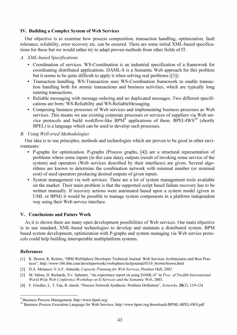
IV. Building a Complex System of Web Services Our objective is to examine how process composition, transaction handling, optimization, fault

tolerance, reliability, error recovery etc. can be ensured. There are some initial XML-based specifica-tions for these but we would rather try to adapt proven methods from other fields of IT. A. XML-based Specifications

• Coordination of services. WS-Coordination is an industrial specification of a framework for coordinating distributed applications. DAML-S is a Semantic Web approach for this problem but it seems to be quite difficult to apply it when solving real problems ([3]).

• Transaction handling. WS-Transaction uses WS-Coordination framework to enable transac-tion handling both for atomic transactions and business activities, which are typically long running transactions.

• Reliable messaging with message ordering and no duplicated messages. Two different specifi-cations are born: WS-Reliability and WS-ReliableMessaging.

• Composing business processes of Web services and implementing business processes as Web services. This means we use existing corporate processes or services of suppliers via Web ser-vice protocols and build workflow-like BPM9 applications of them. BPEL4WS10 (shortly BPEL) is a language which can be used to develop such processes.

B. Using Well-tried Methodologies Our idea is to use principles, methods and technologies which are proven to be good in other envi-

ronments: • P-graphs for optimization. P-graphs (Process graphs, [4]) are a structural representation of

problems where some inputs (in this case data), outputs (result of invoking some service of the system) and operators (Web services described by their interfaces) are given. Several algo-rithms are known to determine the combination network with minimal number (or minimal cost) of used operators producing desired outputs of given inputs.

• System management via web services. There are a lot of system management tools available on the market. Their main problem is that the supported script based failure recovery has to be written manually. If recovery actions were automated based upon a system model (given in UML or BPM) it would be possible to manage system components in a platform independent way using their Web service interface.

V. Conclusions and Future Work As it is shown there are many open development possibilities of Web services. Our main objective

is to use standard, XML-based technologies to develop and maintain a distributed system. BPM based system development, optimization with P-graphs and system managing via Web service proto-cols could help building interoperable multiplatform systems.

References [1] K. Brown, R. Reinitz, “IBM WebSphere Developer Technical Journal: Web Services Architectures and Best Prac-

tices”, http://www-106.ibm.com/developerworks/websphere/techjournal/0310_brown/brown.html [2] D.A. Menascé, V.A.F. Almeida, Capacity Planning for Web Services, Prentice Hall, 2002 [3] M. Sabou, D. Richards, S.v. Splunter, “An experience report on using DAML-S” in Proc. of Twelfth International

World Wide Web Conference Workshop on E-Services and the Semantic Web, 2003. [4] F. Friedler, L. T. Fan, B. Imreh, “Process Network Synthesis: Problem Definition”, Networks, 28(2), 119-124

9 Business Process Management, http://www.bpmi.org/ 10 Business Process Execution Language for Web Services, http://www.bpmi.org/downloads/BPML-BPEL4WS.pdf

RSA TIMING ATTACK BASED ON LOGICAL EXECUTION TIME Csilla ENDRİDI

Advisors: Endre SELÉNYI, Zoltán HORNÁK

I. Introduction Nowadays it is a must to use only those cryptography algorithms, which have been mathematically

accurately analyzed and accepted; but this fact in itself does not mean vested guarantee for the security level provided by a cryptography module. Other – not mathematical – attacks may work so far, where attacker can exploit implementation-dependent features. The so-called side channel attack is based on measuring of side-effects during the operation – e.g. execution time, power, electromagnetic emission –, where using this extra information the secret may be concluded.

Timing attack utilizes that the execution times may be different, and may depend on the used key and the topical message and maybe other facts. With exact knowledge of the source code and the running environment, this dependency can be mapped and for certain crypto algorithms a method for determining the secret key can be worked out. Among others, certain implementation of RSA, Diffie-Hellman, DSA and RC5 are affected by this type of attack [1].

Practical risk of this type of attack is shown by two factors: first, the attack needs only the passive eavesdropping of the channel. Further, the attacking method is quite efficient – in an existing RSA timing attack [2], some ten thousand observations (execution times of cryptography operation on given messages) are enough to find out the secret key with good chance. The execution time of the attacking method depends on only the square of the keysize, thus this method can be qualified as a substantive attack.

II. Vulnerability of the Cryptographic Algorithms The target of timing attack is mostly the modular multiplication, which is often implemented in

practice by the Montgomery algorithm [3]. Its speciality is that the execution always keeps for the same times, expect the only one case, when the result would be greater than the modulus, so a final subtraction (called reduction) is needed. Although modular exponentiation commonly implemented by some kind of fast exponentiation method and not by the repetition of modular multiplications, the attack can be transferred for these algorithms, too.

Although already there are such modular multiplication algorithms, which reduce these threats [4], several, mainly former implementations apply the original Montgomery algorithm. There is another way to protection technique, the so-called blinding [5], which does not require the modification of the algorithm – but causes some decay in efficiency. It is based on a message transformation before the cryptographic operation (and a re-transformation after it), whereby an eavesdropper will not know, on which bits were the algorithm executed – what would be essential for the attack. Regrettably, according to several surveys, in practice this solution also is not applied commonly.

III. Model for Analyzing Timing Attack Our goal was determine if an existing device is affected or not and if so how serious the problem

is. For this reason, we have developed a formal model and a modified timing attack method. We intend to determine the boundary conditions and efficiency properties of the timing attack – e.g. how many observations are needed for success with ε probability.

Our model is general within certain limits: it respects for only those types of algorithms, which uses the secret key only in a loop, consumes its bit one by one, and there is a conditional branch depending on the topical key bit. Most fast exponentiation methods – used by e.g. many RSA coders – are such. The attacking method re-plays the whole cryptography operation step by step, and in each step determines the current key bit. The decision is based on the statistical correspondence between the full and partial execution times. In each step, with ‘0’ and ‘1’ key bit different commands are executed, which keeps for different times. The deviations of the full execution times are aggregated from these elemental deviations, so if we have large number of messages, statistical correspondence must be stand.

Our timing attack method is basically similar to this technique, but in order to carry out more exact observations and reach clearer conclusions, we varied it in three main points.

(1) Instead of measuring real, physical time – such in previous methods – we introduced the notion of logical time: we have assigned a certain “cost” for each command. The costs of the executed commands can be summarized without any noise. While the costs can be set for any value, arbitrary environment or any hypothetical system can be also simulated this way.

(2) With logical time, it is possible to know the costs of each individual steps of the algorithm. It is important, while the exposition of the secret key is based on the deviation of partial execution times. In former methods, only the full times were known, what could cause more obscurity.

(3) We sustain certain number of key-candidates instead of only one potential champion. Such a way, for the success of the attack we don’t have to make right decision in each step; it is enough that the wanted key remains amongst the candidates. Keeping on only certain number of candidates prevents from the state-space explosion, but the efficiency of the algorithm is significantly enhanced.

The most important part of the attack is the candidate-choosing method. At first we generate the potential new candidates by appending ‘0’ and ‘1’ to the former ones. Then assign a goodness-factor for each candidate and keep only the best half of the candidate set. The goodness-factor is a well-defined value describing the correspondence between the partial and full execution times.

IV. Further Tasks The next task is to execute a large number of measurements and to evaluate them. Besides, the

model and the attacking method also can be developed. Further challenge can be: • Introduce the noise into the model; • Examine other candidate-choosing methods and goodness-factors; • Expand the model for more general algorithms; • Adopt the attacking method for protocols, which use the affected algorithms (e.g. SSL).

References [1] P. Kocher, “Timing attacks on implementations of Diffie-Hellman, RSA, DSA, and other systems,” in Advances in

Cryptology – CRYPTO ’96, Santa Barbara, California, vol. 1109 of LNCS, pp. 104-113. Springer, 1996. [2] J. F. Dhem, F. Koeune, P-A. Leroux, P. Mestré, J-J. Quisquater, J-L. Willems, “A Practical Implementation of

Timing Attack,” in Smart Card – Research and Applications, vol. 1820 of LNCS, pp. 175-191. Springer, 2000. [3] P. Montgomery, “Modular Multiplication without Trial Division,” Mathematics of Computation, pp. 519-521, 1985. [4] G. Hachez, J-J. Quisquater, “Montgomery Exponentiation with no Final Subtraction: Improved Results,” in

Proceedings of Cryptographic Hardware and Embedded Systems, vol. 1965 of LNCS, pp. 293-301. Springer, 2000. [5] Dr. Burt Kaliski, “Timing Attacks on Cryptosystems,” RSA Bulletin No.2, Jan. 23. 1996.

Loop

for (i = 1 to n)

IF θ(ki,msg)THEN

Pre

Post

A

B

Figure 1: Our Model

Figure 2: Execution Times

GENERAL-PURPOSE SECURE ANONYMITY ARCHITECTURE Gergely TÓTH

Advisors: Zoltán HORNÁK, Ferenc VAJDA

I. Introduction The rapid development in the area of computer science, hardware, software and communication

systems made it possible to integrate information systems in a constantly increasing factor. This tendency together with the spreading of Internet sets newer and newer challenges for the information science. For the first problems of bandwidth and reliable data transfer several general architectural solutions exist. However nowadays new needs arise: besides the given features secure communication is also required. In the field of encryption, integrity-protection or non-repudiation honored solutions are already known (such as SSL), but their integration with anonymity methods is neither complete nor standardized.

The latest development brought the protection of personal data – privacy – into the spotlight. As larger and larger databases get connected and made – partially publicly – searchable, more and more information about people can be collected. As a sort of countermeasure, anonymity is required in order to hide the identity.

For providing anonymity several different techniques exist. But we lack their uniformity and the means of integrating them into a general system. They can basically be grouped into two categories:

• Anonymous handshaking schemes: with the help of an anonymity authority they make possible for a service provider to be certain that an anonymous subject is authorized to use a specified service. Typical application areas are: anonymous electronic payment (subject is the client, anonymity authority is the bank and the authorization is the payment) [1] or anonymous electronic voting (subject is the voter, anonymity authority is the issuer of the ballot and the service provider is the electronic ballot-box). Anonymous transport is required in the most cases for the anonymous authorization to work properly.

• Anonymous transport methods: in the communication between the subject and the service provider they make the subject’s location anonymous, thus he cannot be traced back. Typical applications are anonymous electronic mailing [2] or anonymous on-line web-surfing [3].

II. Requirements An architecture is needed that provides security functions, guarantees the anonymity of the subject

and incorporates a general framework for the usage of anonymous authorization schemes. These three aspects have to be easily employable from the application layer. An important restriction is that by moving to this new architecture existing applications should need the least possible level of modification. Optimally existing applications should be able to use the new architecture without modifications.

III. Architecture A. Aim

In the field of anonymity we lack a framework that incorporates all required aspects. The general-purpose secure anonymity architecture aims to address this problem by providing an environment, where different anonymity techniques can be implemented and scientifically analyzed.

B. Description A general-purpose secure anonymity architecture (see Figure 1) answering the requirements above

was designed with the considerations below in mind:

TCP/IP

AnonymousHandshake

(AH)Application

Anonymous DatagramLayer (ADL)

Anonymous Session

Layer (ASL)

Securitylayer

Encrypts and relays messages through intermediatenodes, thus provides location anonymity

Enables anonymous replies, thus provides anonymous bi-directional streams

Provides (encryption, integrity protection,authentication, etc.)

security

Provides (e.g. e-voting, e-payment)

application-level anonymity services

Figure 1: General-purpose secure anonymity architecture

The standard TCP/IP protocol of the Internet was used for data transmission. However, since between the user and the service provider no direct TCP/IP connection may exist (from the IP address the user could become back-traceable) the Anonymous Datagram Layer (ADL) has to be introduced. The purpose of this layer is to ensure that messages sent by a user cannot be linked to him. This is achieved by introducing several relay nodes in the network, which mix and encrypt messages of several different users (with the help of cryptographic algorithms) and thus obfuscate the traffic.

In order to enable stream connection between the user and the service-provider, thus making it possible for the service provider to address the user even though it does not know his address, the Anonymous Session Layer (ASL) has to be introduced into the hierarchy.

On top of ADL and ASL a standard security layer can be inserted. Since several anonymity scenarios (electronic voting or on-line payment) require confidentiality, integrity or non-repudiation, one of the commonly used security layers (such as SSL or TLS) should be used.

Finally Anonymous Handshake is introduced in order to realize the anonymous authorization. For this purpose AEP (Anonymity Enhancing Protocol, [4]) can be used.

The architecture defines solely requirements and the service primitives (thus the functionality) for the layers mentioned above, several different techniques and protocols could be used for the implementation.

IV. Conclusion The general-purpose secure anonymity architecture incorporates both security features (such as

confidentiality, integrity or authentication) and anonymity measures (for transparent anonymous communication and authorization).

References [1] D. Chaum, Blind Unanticipated Signature Systems, U.S.Patent 4 759 064, 1998. [2] D. Chaum, “Untraceable Electronic Mail, Return Addresses, and Digital Pseudonyms”, Communications of the

ACM, volume 24, number 2, pp. 84-88, 1981. [3] Anonymizer.com – Online Privacy Services, http://www.anonymizer.com [4] G. Tóth, Anonymity Enhancing Protocol, Ms.E. thesis., Siemens-Award 2002. [5] G. Tóth, Z. Hornák, “Measuring Anonymity”, IWCIT’03

OBJECTIVE EVALUATION OF THE TREMOR Károly János BRETZ

Advisor: Ákos JOBBÁGY

I. Introduction Tremor (shaking) is defined as an involuntary, rhythmic shaking movement of a part of the body

caused by undesirable muscle contractions. Physiologic tremor is a normal, asymptomatic phenomenon present in everyone. Muscle tension increases are followed by increases of amplitudes in the oscillation of forearm and hand.

The present work was designed to discuss methods, investigating and evaluating tremor parameters. The purpose of our presentation is to describe technical solutions, review of measuring equipment and correlation analysis of results gained on healthy subjects. Additional data were provided recording disjunctive reaction times, pulse rate, as well as psychological test applying questionnaire.

Great importance can be attached to tremor investigations at special working conditions of high accuracy manipulations.

II. Methods Electronic equipment was developed for measurements of hand tremor [5]. The equipment

includes digital electronic unit comprising WH1602A-YYB-EP Winstar display with 2 x 16 characters. The design is based on a PIC16F877 microcontroller, providing records and evaluation of tremor parameters as well as the biofeedback functions, to which the AS7C256A SRAM for data storage, the octal bi-directional transceiver, bus line driver, the CD74HC574 LED driver, and the Maxim RS-232 driver-receiver for the PC are connected.

The mechanical part of the equipment includes a receiving unit that makes possible the measurement of tremor, setting different difficulty requirements and adapters, which are tool models, namely miniature soldering iron, as well as screwdriver used by watchmakers. The tremor was evaluated recording two data: the sum of the contacts, namely: when the screwdriver model, driven into the bore of the front plate, touched the plate; as well as the sum of contact times.

The equipment is capable of recording parameters for investigations of skill in the industry. Suitable applications include screening of candidates, applying for jobs where use of precision instruments and electronics is important, as well as for the examination of patients to distinguish their pathological tremors.

Pulse rate and disjunctive reaction times were recorded applying "Psycho 8" device. Combinations of sixty stimuli and responses were used. Red and green LEDs provided light stimuli. "A" and "B" errors were recorded. The sense of "A" type error: the subject did not respond to the stimulus. The meaning of "B" type error: the subject reacted faultily. Complementing and synchronizing the equipment, 50 and 100 Hz sampling frequencies will be set. Using the above-described devices, data were collected on thirty-six college students who participated in this study by appointment.

Subjects began with filling out the questionnaires, namely a test anxiety inventory and performed a tremor test. After this the disjunctive reaction time and the pulse rate were measured.

III. Results In our preliminary investigations significant correlation (p<0,05) was found between:

• tremor and pulse rate (+) (females), • tremor, emotional excitement (TAI/E) (+) (males), • pulse rate and emotional excitement (TAI/E) (+) (males and females), • pulse rate and reaction time (-) (females),

TAI/E: emotional excitement. It is defined by the numerical result of test using questionnaire

developed by Spielberger [1].

IV. Discussion and Conclusion Diagnostics have interest in getting to know the cause, but the tremor is an effect. Although the

tremor was considered an objectively measurable physiological parameter, problems can occur investigating the cause and in classification of tremor occurence.

No doubt that emotional disturbances have impact on tremor and examination results. In our investigation the healthy excitement was a drive, which was necessary for mental and experimental work. It was expected that higher pulse rate could be found in such case.

The presentation will outline the other parts of the equipment, partially under development at present: the stabilometry device, the laser transmitter and receiver unit, as well as the electronic adapter providing synchronization of devices.

References [1] C.D. Spielberger, Preliminary professional manual for the Test Anxiety Inventory (TAI). Consulting Psychologist

Press. Inc. Palo Alto, CA. 1980. [2] J. Ghika, A. W. Wiegner, J. J. Fang, “Portable system for quantifying motor abnormalities in Parkinson's disease”,

IEEE Transactions on Biomedical Engineering. 40. 276–283, 1993. [3] R. Edwards, A. Beuter, “Indexes for identification of abnormal tremor using computer tremor evaluation systems”,

IEEE Transactions on Biomedical Engineering, 46. 895–898, 1999. [4] J. M. Spyers–Ashby, M. J. Stokes, “Tremor. Physiological aspects, movement disorders”, Clinical Rehabilitation,

14(4) 425–433, 2000. [5] K. J. Bretz, K. Sipos, “Tremor and stress during college examination”, Kalokagathia, 41(1): 111–115, 2003. [6] G. Rao, L. Fisch, S. Srinivasan, F. D'Amico, T. Okada, C. Eaton, C. Robbins, “Does this patient have Parkinson

disease?” JAMA 289(3). 347–353, 2003.

MICROCALCIFICATION DETECTION USING NEURAL NETWORKS

László LASZTOVICZA Advisor: Béla PATAKI

I. Introduction Breast cancer is a common form of cancer among women. The cause of this illness is unknown so

prevention is not possible. The only way for an effective treatment is to detect the disease in its early state. Mammography is the best known method for early detection [1]. In a mammographic session at least four x-ray images are taken and in order to make a reliable diagnosis each image have to be evaluated. The evaluation process requires a large amount of human resources and money. The main goals of a supporting computer-aided diagnosis (CAD) system are to increase the effectiveness of the examination by drawing radiologists’ attention to the suspicious cases and to decrease the costs by filtering out normal images. One of the most important symptoms of cancer is the presence of microcalficitions. The subject of

this article is to present a method for detecting microcalcifications. This method uses neural networks to perform this task.

II. A Neural Method for Microcalcification Detection The microcalcifications as objects in the images are very diverse in size, shape and brightness so

an exact detection criterion cannot be given easily. Neural networks have been proven to be useful in the solution of such pattern recognition tasks. We used a previously presented [2] hierarchical neural network architecture with some modifications and extensions [3]. This architecture is shown in Figure 1.

Figure 1: A hierarchical neural network architecture This architecture is based on a multiscale decomposition of an image, and a hierarchy of neural

networks. First the input image is sampled and an image pyramid is built, where the resolution is halved at each level. Next a number of features are extracted from each image. The processing works pixel-by-pixel so the feature extraction assigns a vector for each pixel. The last step is the neural classification that is based on the vectors resulted from the feature extraction. This architecture was extended with a decision system, which uses the output of the networks and some of the input

Neural network #1 Neural

network #2 Neural

network #3

Image pyramid Feature extraction Neural classification #1

Processing directions

Output

Hierarchical Neural Network

features to make a decision about the whole input image. Further extension is that this architecture was embedded in an ensemble context that is several differently trained neural networks are used instead of one. If we consider the ensemble and the decision system as a module, than we can modularize the system. Each module uses a different set of parameters for the feature extraction task. The goal of modularization is to further improve performance and robustness of the solution [3].

III. Experimental Analysis The performance of the system was analyzed on two different image databases. The neural

networks, the decision system and the location procedure were thoroughly tested in the experiments. The results show that the system is capable of detecting microcalcifications, however the parameters of the system should be changed in order to ensure the same performance. We experienced that the decision system is much more sensitive to the circumstances than the neural networks and therefore it should be reconsidered in the future research. The performance of the system on 6440 ROIs (regions of interest) extracted from the first database

was 82% true positive and 72% true negative. There are only preliminary tests on the second database, which has better resolution. These show that the neural networks detect most of the calcifications without the need of retraining, but the decision system performs poorly. The test set contained 1600 ROIs extracted from different images containing microcalcifications. The neural networks detected almost all of the calcifications while the decision system marked the ROIs as positive in less than 10% of the cases. Some results can be seen in Figure 2.

Figure 2: Some results of the system

IV. Conclusion and Future Work A neural network based system has been presented that is capable of detecting microcalcifications.

The thorough analysis of this system showed that its parameters are sensitive to the properties of the images like the size or the resolution. This stands especially to the decision system. The future work includes the analysis of neural learning, which has central influence on the

performance, and the improvement of the decision system to decrease its sensitivity toward the parameters of the images.

References [1] R. Highnam, M. Brady, Mammographic Image Analysis, Kluwer Academic Publishers R, 1999. [2] P. Sajda and C. Spence, “Learning Contextual Relationships in Mammograms using a Hierarchical Pyramid Neural

Network”, IEEE Transactions on Medical Imaging 21(3), 2002. [3] László Lasztovicza, Béla Pataki, Nóra Székely, Norbert Tóth, “Neural Network Based Microcalcification Detection

in a Mammographic CAD System”, Proceedings of the Second IEEE International Workshop on Intelligent Data Acquisition and Advanced Computing Systems: Technology and Applications (IDAACS'2003), pp. 319-323, Lviv, Ukraine, 8-10 September, 2003.

TEXTURE ANALYSIS OF MAMMOGRAMS

Norbert TÓTH Advisor: Béla PATAKI

I. Introduction Breast cancer is the most common form of cancer of women. According to statistics, one out of

every eight women will develop breast cancer in her lifetime. Thanks to recent advances in medicine, there are more and more effective methods in the treatment of breast cancer. Since the cause of breast cancer is unknown, early detection is very important. If detected early, the five-year survival rate exceeds 95%. A mammogram is an x-ray picture of the breasts. It is used to detect tumors and cysts and to help

differentiate between benign (non cancerous) and malignant (cancerous) cases. The success of treatment depends on early detection. Mammography can show changes in the breasts well before the patient recognizes it.

II. The Proposed System The efficiency of mammography is based on the success of separating the different types of

tissues. Texture analysis [5] allows us to segment the image and classify the segmented regions. These regions can be used to form a diagnosis or can be the inputs of forthcoming methods. In this study a complex system (Fig. 1) for mammographic texture analysis is presented. The

system consists of preprocessing, image enhancement, feature extraction, parameter adaptation, “coarse” and “fine” segmentation. The algorithm presented in this paper uses the intensity co-occurence matrix [1], Gabor filters [4]

and gray level run length properties [5] to obtain the image features used for texture descriptors. These features are then passed to a decision tree, which classifies the actual image segment to form the “coarse” segmentation. Image segments are cut from the original image using a sliding window. This segmentation method gives a rough representation of the quantity and localization of the tissues in the breast according to the actual window size. This preliminary segmented image is used as a starting point for a second algorithm (using a Markov Random Field [2] [3]) to obtain “fine” segmentation. This method models the segmented image as a Markov random field, and the original image (in our case the mammogram) as the segmented image with additive Gaussian noise. The optimization uses ICM (Iterated Conditional Modes) to approximate the MAP (Maximum A Posteriori) segmentation of the image. The system includes a preprocessing step (to extract the breast from the surrounding background

and to remove any object in the image that is not part of the breast itself using standard thresholding and median filtering [5]) and an image enhancement step (using histogram equalization [5]) to unify the intensity range of the images. Parameters for the segmentation algorithms are determined in a preliminary step, using supervised

learning. This step uses a learning set of images (both original and segmented) to create a decision tree that will cluster the feature vectors of the different textures (“coarse” segmentation). Some further parameters (e.g. random field and image model parameters) are also determined from the training samples.

Figure 1: The texture analyzing system and sample images

III. Preliminary Results and Conclusion A complex system (Fig. 1) for mammographic texture analysis is proposed in this study.

Preliminary results of the proposed complex system are promising. 16 images were tested, each containing one lesion. During texture analysis, 2 of the 16 lesions were lost (87% TP ratio). Since these results are only preliminary, a large scale test and a detailed discussion of the results will be finished in the next weeks.

References [1] J. Iivarinen, Texture Segmentation and Shape Classification with Histogram Techniques and Self-Organising Maps,

Acta Polytechnica Scandinavica, No 95, TTA, Helsinki, 1998. [2] H. D. Li, M. Kallergi, L. P. Clarke, V. K. Jain, “Markov Random Field for Tumor Detection in Digital

Mammography”, IEEE Transactions on Medical Imaging, vol. 14, no. 3, pp. 565-576, September 1995. [3] S. Z. Li, Markov Random Field Modeling in Computer Vision, Springer-Verlag, New York [etc.], 1995. [4] Stéphane Mallat, A Wavelet Tour of Signal Processing, University Press, Cambridge, 2001. [5] I. Pitas, Digital Image Processing and Algorithms and Applications, John Wiley & Sons, New York, 2000.

„coarse” segmentation

segmented training image

Determine decision tree and other parameters

SUPERVISED TRAINING IMAGE

ORIGINAL IMAGE

IMAGE ENHANCEMENT

PREP ROCESSING

FEATURE EXTRACTION

„Fine” segmentation using Markov Random Field

„Coarse” segmentation using decision

tree

SEGMENTATION

Parameter approximation

original image preprocessed image enhanced image

„fine” segmentation

TUMOR DETECTION ON PREPROCESSED MAMMOGRAMS

Nóra SZÉKELY Advisor: Béla PATAKI

I. Introduction Breast cancer has become one of the leading mortality causes among women [1]. The chance of

survival significantly grows if it is detected early; so a screening program was started in 2002. The high number of mammograms requires computer-aided diagnostics. The main goal is to help the work of radiologists by finding true negative cases, thus they only have to examine suspected positive ones. So the detection ratio of true positive cases must be as high as possible, while the ratio of false positive detections must be kept at a low level to avoid unnecessary examinations. Tumors are difficult to describe by mathematical models, and conventional image processing

methods also fail to detect them, so a combined technique is being developed. First global methods are used to obtain a segmentation of breast tissues. They can extract some suspicious areas in the breast, but they generally find at least 3-4 such places in every image, so the ratio of false positive detections (FPR) becomes impermissibly high. Thus local methods are used to reduce this FPR. In this work these local methods are discussed, and the achieved results are presented, respectively.

II. Local Methods Accepting a candidate as a real tumor or rejecting it consists of three steps. First segmentation is

performed to obtain a black-and-white mask of the candidate, and then some parameters are calculated using this mask. The final decision is then made on the basis of these parameters. A. Segmentation Three methods are combined, namely dual binarization, the Bèzier histogram method [2,3] and a

modification of the radial gradient index (RGI) method [4]. The RGI method works as follows: the patch is multiplied by a Gaussian function to constrain the candidates to have circular shape and then this modified patch is binarized by several thresholds. The border of the resulting objects is examined using the original patch. That object is chosen, of which border minimizes Eq. (1).

dyxG

yxGyxryxryxG

RGI Hyx

Hyx

Hyx∑

∑∑

∈

∈

∈ −= ),(

),(

),(),(

),(),(),(),(

, (1)

where H is the border of the object, r(x,y) is the radius, G(x,y) is the gradient at (x,y) and d is the number of points in the border. The second term of (1) was not used in the original equation, but it proved to be useful as a regularization member (see Fig. 1). The first part says that gradients must point towards the center point, the second that they must be high.

Figure 1: RGI method (a) Original patch, (b) RGI with regularization, (c) RGI in its original form

As a result of segmentation a black-and white mask is obtained that is used to calculate several parameters of the image patch. B. Parameters Some parameters refer to the shape of the object; the others are texture features. They are:

compactness (square of the length of the perimeter divided by the area) [5]; moments [6]; a special symmetry measure based on PCA [2,3]; average brightness of the masked area; average brightness of the background (unmasked area); the ratio of these two measures; average variance of the masked area; average variance of the background. C. Making the Final Decision Parameters were handled two ways: we used them in their original form, and we applied PCA to

make them uncorrelated. In both cases, those parameters were taken into consideration first which correlated best to the desired output. A further goal is to build an automatic clustering module.

III. Results Since currently there is no available reliable global segmentation, the testing was performed on a

special database, which contained all the tumors cut from the original images and randomly cut patches from the normal mammograms. This task is relatively easy, because when using globally segmented images, candidates are all “tumor-like” and not random. The original mammograms are from the DDSM database [7].

Table I. Preliminary results #Patches #Tumors TP ratio FP ratio

Original Parameters 8630 2241 94.5% 12.8%PCA parameters 8630 2241 95.3% 24.5% The achieved results are promising, because even radiologists miss 10% of positive cases.

IV. Conclusion Since there is no currently available mathematical description of the tumors in mammograms, and

detecting them is a very complex task, a combined technique is being developed using global and local methods. Global methods are used to find regions of interest in the mammograms, then some local methods make the final decision whether the candidate is truly a tumor or not. Preliminary results are promising; a large test using globally segmented mammograms is currently in progress.

References [1] R. Highnam, M. Brady, Mammographic Image Analysis, Kluwer Academic Publishers, 1999. [2] N. Székely, B. Pataki, ”Detecting Lesions in a Mammogram”, in Proc. of EC-VIP-MC 2003 4th EURASIP

Conference focused on Video/Image Processing and Multimedia Communications, pp. 113–118, Zagreb, Croatia, July 2–5 2003.

[3] H. Qi, W. E. Schneider, “Lesion detection and characterization in digital mammography using Bèzier histograms”, SPIE Medical Imaging: Image Processing, Pt.1–2, pp. 1521–1526, Feb. 1999. URL: http://aicip.ece.utk.edu/publication/99spie_lesion.pdf.

[4] M.A. Kupinski, M.L.Giger, “Automated Seeded Lesion Segmentation on Digital Mammograms”, IEEE Tr. on Medical Imaging, 4:510–517, 1998.

[5] L. Shen, R. M. Rangayyan, J. E. L. Desautels, “Application of Shape Analysis to Mammographic Calcifications”, IEEE Tr. On Medical Imaging, 13(2):263–274, June 1994.

[6] R.C. Gonzalez, R.E. Woods, Digital Image Processing, Addison-Wesley Publishing Company, 1993. [7] M. Heath, K.W. Bowyer, D. Kopans et al, “Current status of the Digital Database for Screening Mammography”,

pp. 457-460 in Digital Mammography, Kluwer Academic Publishers, 1998.

� ������� ���� �� ��� �� �������������� ������

������������� ��� ������������ ����� ���� ���� ��������

������������� �������� ����� � ��������� �����

!������� "� ���# $���� ��"���

�������� %&' ���������(��

� ������� ��� � �)���� � ��������� *����� ��������

!������� "� ���# !��� +��

������ ���# ,�-./'

���� ��� � ��

���� ��� � ��