Embed Size (px)
Citation preview

PROCEDURE TO QUANTIFY ENVIRONMENTAL RISK OF NUTRIENT LOADINGS TO SURFACE WATERS
Tone Merete Nordberg
Thesis submitted to the Faculty of Virginia Polytechnic Institute and State University in
partial fulfillment of the requirements for the degree of
Master of Science
In
Biological Systems Engineering
Mary Leigh Wolfe (Chair)
Darrell J. Bosch
David F. Kibler
February 9, 2001
Blacksburg, Virginia
Keywords: Environmental Risk, Phosphorus, Dissolved Oxygen, ANSWERS-2000, HSPF

Tone Merete Nordberg Table of Contents BSE
ii
PROCEDURE TO QUANTIFY ENVIRONMENTAL RISK OF NUTRIENT LOADINGS
TO SURFACE WATERS
Tone Merete Nordberg
(ABSTRACT)
Agricultural production and human activities in a watershed can expose the watershed to
environmental degradation, pollution problems, and a decrease in water quality if resources and
activities within a watershed are not managed carefully. In order to best utilize limited resources
and maximize the results with respect to time and money spent on nonpoint source (NPS)
pollution control and prevention, the environmental risk must be identified so that areas with a
higher quantified environmental risk can be targeted. The objectives of the research presented in
this master thesis were to develop a procedure to quantify environmental risk of nutrient loadings
to surface waters and to demonstrate the procedure on a watershed.
A procedure to quantify environmental risk of nutrient loadings to surface waters was
developed. The risk is identified as the probability of occurrence of a nonpoint source (NPS)
pollution event caused by a runoff event multiplied by the consequences to a biological or
chemical endpoint. The procedure utilizes the NPS pollution model ANSWERS-2000 to generate
upland pollutant loadings to receiving waters. The pollutant loading impact on stream water
quality is estimated using the stream module of Hydrologic Simulation Program FORTRAN
(HSPF). The risk is calculated as the product of probability of occurrence of a NPS event and
consequences of that event.
The risk quantification procedure was applied to a watershed in Virginia. Total phosphorus (TP)
loadings were evaluated with respect to resultant in-stream dissolved oxygen (DO)
concentration. The TP loadings were estimated in ANSWERS-2000 then the consequences were
estimated in HSPF. The results indicated that risk was higher for the smaller, more frequent
storms indicating that these smaller, more frequent loading events represent a greater risk to the

Tone Merete Nordberg Table of Contents BSE
iii
in-stream water quality and ecosystem than larger events. While the probability of occurrence of
lower TP loading was higher because they were caused by smaller, more frequent storms, the
consequences were less for the same events.
The developed procedure can provide watershed stakeholders and managers with a useful tool to
quantify the environmental risk a watershed is exposed to as a result of different land
management and development scenarios. The scenarios can then be compared to identify a risk
level that is considered acceptable. The procedure can also be used by policymakers to set a cap
on the risk a certain activity can expose a watershed to.

Tone Merete Nordberg Table of Contents BSE
iv
Acknowledgements First and foremost I would like to thank my parents, Signe and Harald for their endless support
during my education. They thought me the importance of education and guided me to values and
believes in life that has enabled me to accomplish everything I set out to do. For that I am forever
grateful, Thank you !!
A special thanks also goes to my advisor, Dr. Mary Leigh Wolfe, for her guidance and support
throughout my graduate studies. She was always there to guide me in the right direction when I
lost my compass and she helped me grow as a student and as a person.
I would like to thank Tamie for all the help she gave me debugging and correcting my code when
my programming skills did not hold up.
I would also like to thank all my friends in Blacksburg, especially Alex, and Eirik in Trondheim
for all the happy memories and late nights we had together, and hope there will be many more
throughout life.
And finally a very special thanks to Chittiappa, for always lending an ear when things were not
going my way, for motivating me, for cooking me dinner, for making the best Sunday breakfasts,
and for always being there for me.
Tone.

Tone Merete Nordberg Table of Contents BSE
Table of Contents
ABSTRACT) ...................................................................................................................................ii
Acknowledgements .........................................................................................................................iv
Table of Contents.............................................................................................................................v
List of Figures ................................................................................................................................ vii
List of Tables ................................................................................................................................ viii
1.0 Introduction............................................................................................................................... 1
1.1 Research Objective ............................................................................................................... 2
2.0 Literature Review...................................................................................................................... 3
2.1 Introduction........................................................................................................................... 3 2.2 Risk and Risk Assessment .................................................................................................... 3 2.3 Probability Concepts ............................................................................................................. 6 2.4 Application of Environmental Risk Assessment with Respect to Water Quality................. 6 2.5 Phosphorus Loadings Implications on Water Quality .......................................................... 9 2.6 Summary of Literature Review........................................................................................... 13
3.0 Development of Risk Quantification Procedure ..................................................................... 15
3.1 Introduction......................................................................................................................... 15 3.2 Conceptual Procedure Development ................................................................................... 15 3.3 Procedure Implementation.................................................................................................. 17
3.3.1 Introduction.................................................................................................................. 17 3.3.2 Upland NPS Model Selection...................................................................................... 17 3.3.3 Stream Model Selection............................................................................................... 19 3.3.4 Weather Data Preparation............................................................................................ 21 3.3.5 ANSWERS-2000 Modeling......................................................................................... 26 3.3.6. From ANSWERS-2000 Output to HSPF Input .......................................................... 26 3.3.7 HSPF Modeling ........................................................................................................... 27 3.3.8 Risk Quantification...................................................................................................... 28
3.4 Summary of Procedure Implementation............................................................................. 31
4.0 Application of Procedure ........................................................................................................ 32
4.1 Introduction......................................................................................................................... 32 4.2 Test Watershed Selection.................................................................................................... 32
4.2.1 Endpoint Selection....................................................................................................... 34 4.3 Lola Run Landuse ............................................................................................................... 35 4.4 Lola Run Soils..................................................................................................................... 37 4.5 Lola Run Fertilizer Applications ........................................................................................ 38

Tone Merete Nordberg Table of Contents BSE
vi
4.5 Weather Data....................................................................................................................... 39 4.6 ANSWERS-2000 Modeling of Lola Run ........................................................................... 41 4.7 HSPF Modeling .................................................................................................................. 44 4.8 Risk Analysis Results ......................................................................................................... 46
5.0 Potential Applications of the Risk Quantification Procedure ................................................. 50
5.1 Introduction......................................................................................................................... 50 5.2 Applicable Uses of the Risk Quantification Procedure ...................................................... 50
6.0 Summary and Conclusions ..................................................................................................... 53
References ..................................................................................................................................... 55
APPENDIX A: Percent Cloud Cover Calculations ............................................................... 62
APPENDIX B: HplotEnglish Source Code........................................................................... 73
APPENDIX C: MutReader Source Code .............................................................................. 82
APPENDIX D: RiskCalc Source Code ................................................................................. 86
APPENDIX E: ANSWERS-2000 Output ............................................................................. 91
APPENDIX F: F-tables calculations ................................................................................... 116
APPENDIX G: Travel time calculations ............................................................................. 126
Vita.............................................................................................................................................. 126

Tone Merete Nordberg List of Figures BSE
List of Figures Figure 3.3.8.1 Schematic of risk quantification procedure………………………………….. 28
Figure 3.3.8.2 Schematic of linking ANSWERS-2000 output to HSPF output…………...… 30
Figure 4.2.1 Location of Lola Run watershed within Muddy Creek……………………... 33
Figure 4.2.2 Lola Run outlet into Muddy Creek…………………….…………………… 34
Figure 4.2.3 Lola Run looking upstream from output…………………………………….. 34
Figure 4.2.4 Lola Run flowing through a field looking upstream ……………………….. 34
Figure 4.2.5 Smaller tributary to Lola Run ………………………………………….. 34
Figure 4.3.1 Landuse in Lola Run watershed …………………………………………… 35
Figure 4.4.1 Lola Run soils map……………………………………………………………. 38
Figure 4.5.1 Generated annual rainfall data set used in ANSWERS-2000 compared to
observed annual average………………………………………………………. 41
Figure 4.6.1 Subwatershed division of Lola Run………………………………………….. 42
Figure 4.6.2 Sediment loss output from ANSWERS-2000 for Subwatershed 2………… 43
Figure 4.6.3 Dissolved PO4 output from ANSWERS-2000 for Subwatershed 2…………… 44
Figure 4.7.1 Sample output from HSPF from the latter half of November during the 28th
year simulation showing DO and TP concentrations as a function of time……46
Figure 5.2.1 Illustration of risk procedure to evaluate different management practices…… 51
Figure 5.2.2 Screen print of the RiskCalc program……………………………………… 52

Tone Merete Nordberg List of Tables BSE
List of Tables
Table 3.3.3.1 Table 3.3.3.1 Stream model comparison matrix adapted from USGS website (USGS, 2000)…………………………………………….……..… 20
Table 4.3.1 Lola Run landuse categories and areas……………………………………. 36
Table 4.3.2 Landuse and management practices for Lola Run used in
ANSWERS-2000……………………………………………………….. 36
Table 4.4.1: Fertilizer applications used in ANSWERS-2000 for Lola Run Watershed.. 38
Table 4.5.1 Two sided t-test of annual rainfall at Big Meadows weather station……. 39
Table 4.5.2 Mean monthly precipitation for December month for 50 years
of data……………………………………………………………………. 40
Table 4.8.1 Statistical summary of TP loading output from ANSWERS-2000
based on 50 years of simulated weather data……………………………… 47
Table 4.8.2 Results of risk quantification for Lola Run watershed as a result
of TP loadings into the system…………………………………………… 49

Tone Merete Nordberg Chapter 1. Introduction BSE
1
1.0 Introduction
Agricultural production and human activities in a watershed can expose the watershed to
environmental degradation, pollution problems, and a decrease in water quality if resources and
activities within a watershed are not managed carefully. The level of risk exposure in a
watershed must be quantified by widely accepted and measurable parameters in order to properly
manage the environmental risk in the watershed. If this is done successfully, it gives inhabitants
of the watershed a tool to control environmental risk to the ecosystem caused by activities in the
watershed. Guidelines and regulations can then be made based on acceptable risk levels in the
watershed. In order to best utilize limited resources and maximize the results with respect to time
and money spent on nonpoint source (NPS) pollution control and prevention, the environmental
risk must be identified so that areas with a higher quantified environmental risk can be targeted.
The impact of NPS pollution on the environment and the receiving ecosystem must be quantified
in order to identify the risk NPS pollution imposes on the environment and the ecosystem.
In the 1970’s, the early days of environmental law enforcement, a zero-risk approach was often
taken, with the objective of most regulatory policies and plans to eliminate all environmental
degradation and pollution. By the early 1980’s it had become apparent that this zero-risk
approach was impractical and far from being economically viable (Barnthouse et al., 1988). With
this shift towards reducing risk to a socially and environmentally acceptable level, the need for
risk analysis with respect to the environment and the ecosystem became apparent, which led to
what today is known as environmental risk assessment, ecological risk assessment, and
environmental impact assessment.
The concept of risk assessment is a well-known topic in fields like hazardous materials handling
and construction. In calculating risk scenarios for industrial plants and hazardous materials, a
worst-case scenario is often assumed to predict the most extreme risk (Paul, 1996). This method
does not apply readily to NPS pollution risk assessment because NPS pollution is diffuse and
intermittent in nature. In the case of NPS pollution, the continued risk the ecosystem is exposed
to, in terms of the many small and medium rainfall events over a year, is of greater importance to
the overall health of the waterbody than is the maximum risk that occurs with a 100-year storm.

Tone Merete Nordberg Chapter 1. Introduction BSE
2
Hence, it is more appropriate to deal with the issue of risk as a daily-endured risk by the
receiving ecosystem, like the average daily risk to the ecosystem as a result of land management
practices conducted in the watershed. If a relationship between pollutant loadings to surface
waters and environmental risk can be established, it will be possible to quantify impacts of
pollutant loadings in terms of economics or possibly other measures which will further aid in the
process of choosing the best strategy for managing the watershed for all its inhabitants, human
and nonhuman.
1.1 Research Objective
The overall objective of this research was to quantify the environmental risk a waterbody is
exposed to as a result of pollutant loadings to surface water. The developed procedure is intended
to aid in cost-effective environmental risk management for watersheds.
The specific objectives were to:
1. Develop a procedure to quantify the risk of pollutant loadings to surface waters considering
both the probability of loading occurring and loading impact on receiving waters.
2. Apply the developed procedure to a watershed for a specific pollutant.

Tone Merete Nordberg Chapter 2. Literature Review BSE
3
2.0 Literature Review
2.1 Introduction
As stated in the previous section, the overall objective of this research was to quantify the
environmental risk of pollutant loadings to surface waters. The relevant information obtained
from the literature review is presented in the following sections. The first section discusses
definitions of risk with respect to environmental risk assessment and ecological risk assessment.
The second section contains a discussion on various concepts in probability relevant to this
research. In the third section, applications of environmental risk assessment to water quality and
especially phosphorus are discussed. The application of the risk quantification procedure used in
this case study involved the effects of phosphorus loadings on dissolved oxygen concentration in
receiving waters, which are discussed in the last section of this literature review.
2.2 Risk and Risk Assessment
Risk is often defined as the uncertainty concerning an undesired event where uncertainty is
expressed as the probability of occurrence of the event (ASTM, 1985). Risk assessment dates
back to the beginning of the last century when economic risk was the focus. The link to
environmental decision making is much newer. Henley and Kumamoto (1991) defined risk
according to the following equation:
×
=
eventeconsequenc
magnitudetimeunit
eventsfrequency
timeeconsequenc
risk_
[2.2.1]
Whyte and Burton (1980) defined environmental risk as the risk that arises in or is transmitted
through the air, water, soil or biological food chains to humankind. From this definition it is clear
that environmental risk includes a wide range of areas: public health, economic development,
natural resources, introduction of new products and human induced or natural disasters (Whyte

Tone Merete Nordberg Chapter 2. Literature Review BSE
4
and Burton, 1980). The National Research Council defined environmental risk assessment as the
characterization of the potential adverse health effects of human exposure to environmental
hazards (NRC, 1983). Yet another definition was provided by Wilson and Crouch (1987). They
considered environmental risk assessment the use of toxicological and ecological data to estimate
the probability that some undesirable environmental event will occur. While the definition by the
NRC deals strictly with human health, the Wilson and Crouch definition deals with any
undesirable environmental event, which may or may not include human health.
Another closely related field is ecological risk assessment. The two fields are very similar and
very often with similar definition. The USEPA (1988) defined ecological risk assessment as any
assessment related to actual or potential ecological effects resulting from human activities.
Hunsaker et al. (1989) defined regional ecological risk assessment to be concerned with
describing and estimating risk to the environmental resources at the regional scale or risk
resulting from regional-scale pollution and physical disturbance. A few years later, Suter (1993)
defined ecological risk assessment as the process of assigning magnitudes and probabilities to
the adverse effects of human activities or natural catastrophes. Suter added that ecological risk
assessment is risk assessment for the nonhuman environment. In practice, ecological risk
assessment has become the application of the science of ecotoxicology to public policy (Suter,
1993). Ecological risk assessment, though often very similar to environmental risk assessment as
stated earlier, tends to focus on the health of the ecosystem and specific species in the ecosystem
as a response to a pollutant or human activity, whereas environmental risk assessment often is
more concerned with the chemical fate of the pollutants and the pollutant interactions with other
chemicals present.
Environmental impact assessment is a term often used in relation to environmental and
ecological risk assessment. Environmental impact assessment covers a much broader area; it
deals with all aspects and activities involved in the tasks of analyzing and studying the effects of
human activities and actions upon the environment (Suter et al., 1987). These effects are not per
definition negative changes or implications. While dealing with environmental risk assessment
and ecological risk assessment, it is assumed that outcomes of the undesired event are negative.

Tone Merete Nordberg Chapter 2. Literature Review BSE
5
Risk assessment can be defined as the scientific task of assigning probabilities of adverse effects,
while risk management is the task of evaluating the social implications of the risk (Moghissi,
1984). Ruckelshaus (1983) argued the importance of the use of risk analysis, which includes both
risk assessment and management, but he distinguished between the two and argued that risk
assessment is a scientific task, while risk management should be in the hands of decision and
policy makers. Moghissi (1984) reinforced this view, as he argued that separating the two could
result in risk assessment policies that are based on arbitrary decisions rather than scientific
evidence. Risk assessment can seldom rely on complete information. It is often necessary to
make decisions based on incomplete scientific information or based on known scientific basis
but lack of necessary data to support the scientific basis. It is very important however that even
with incomplete information or lack of necessary data that scientific basis be applied to ensure
the best possible and credible outcome (Moghissi, 1984).
Based on this literature review, the following definition was adopted for this work.
Environmental risk was defined as the probability of occurrence of an undesirable event (e.g.
water pollution) multiplied by the consequence of that specific event (e.g. dissolved oxygen),
following the general definition of risk proposed by Henley and Kumamoto (1991). This
definition encompasses some of Whyte and Burton’s (1980) definition concerning natural
resources, while leaving out the human health aspect of environmental risk.
Furthermore, it is important to distinguish between the different components of risk. Natural risk
is the risk endured without human interference, such as the risk to a species in the wild that
naturally occurs due to the stochastic nature of the environment. Anthropogenic risk is the risk
added by human activities and influence. The total risk is then equal to the natural and
anthropogenic risks added together (Power et al., 1994). Law and Kelton (1991) argued that
only models give the statistical and experimental control necessary to estimate both the natural
and anthropogenic risks in a satisfactory way due to the complexity and variability of the system
being modeled. The level of statistical and experimental control that Law and Kelton argued is
not present in most physical experimental frameworks.

Tone Merete Nordberg Chapter 2. Literature Review BSE
6
2.3 Probability Concepts
Estimating the probability of occurrence of an undesirable event is a key component of risk
quantification. Barnett (1992) distinguished three different interpretations of probability;
frequentist, logical and subjective. In a frequentist view, the only information that is regarded
relevant for the probability assessment is obtained from observing the outcomes in repeated
realizations of the fully described experimental process. Hence, probability of a specific outcome
is defined as the total number of times the event occurred in the total number of times the trial
was performed. The logical view expresses the rational or credible extent of belief that a person
puts on the likely occurrence of an event by the available body of knowledge. The logical view
has parallels to the better known ‘weight of evidence’ approach or the rational argument, which
often is used by public interest groups in characterizing environmental risk. Critics of this view
argue that it is not possible to obtain a numerical value of risk with this view and that there is a
lack of common agreement that makes it hard to use. The third view, the subjective view, is
concerned with individual behavior and preferences when confronted with different possible
actions and how individuals reach the judgments. The subjective view can be used to quantify
expert opinion and is applicable in certain risk quantification situations (e.g. yield risk for
farmers). The subjective view is difficult to apply to environmental risk assessment since
interpersonal comparison is very difficult.
2.4 Application of Environmental Risk Assessment with Respect to Water Quality
In the field of hydrologic modeling, uncertainty is divided into three types of uncertainty widely
recognized and discussed by several authors (Haan, 1989, 1977; Hession et al., 1997; Parson et
al., 1998). First is the stochastic nature of the natural environment, the inherent variability in
natural processes. An example of characterizing stochastic uncertainty is the work done by Ünlü
et al. (1990) in which a stochastic analysis of unsaturated flow was performed. The stochastic
behavior of one-dimensional flow was assumed to be a function of soil hydraulic properties,
saturated hydraulic conductivity, pore size distribution and specific water capacity. A Monte
Carlo Simulation (MCS) approach was used to model the flow system. The second type of
uncertainty deals with model uncertainty that arises because it is not possible to know for sure

Tone Merete Nordberg Chapter 2. Literature Review BSE
7
that a hydrologic process is completely or correctly represented in a model. Model uncertainty
will greatly influence the confidence in the output from model simulations. Summers et al.
(1993) discussed a MCS and a first order error propagation method to quantify prediction
uncertainties in water quality models. Chaves and Nearing (1991) applied a modified response
surface technique combined with a modified point estimate method to predict uncertainty in the
WEPP (Water Erosion Prediction Project) model.
The third type of uncertainty is uncertainty in input parameters to models. Parameter uncertainty
represents incomplete information and misrepresentation and misestimation of parameters in a
model. Parameter uncertainty increases as the complexity of a model increases, that is, increased
knowledge about the processes being modeled leads to a greater number of parameters to
estimate, which leads to increased uncertainty about the system. Rowe (1977) used the term
“information paradox” to describe this situation. Kuczera and Parent (1998) used a MCS to
assess the parameter uncertainty in conceptual catchment models. Hession et al. (1997)
considered both the stochastic variability in nature and a combined parameter and model
uncertainty into what was termed knowledge uncertainty.
Risk assessment when hydrologic models or other models are involved should ideally consider
all three types of uncertainty but this is very often not possible due to the resulting overall
complexity of the problem. In this research, the risk assessment was limited to the inherent
variability of natural processes, the stochastic uncertainty in the represented system.
In the early 1990’s, Orvos and Cairns (1991) examined a risk assessment strategy for the
Chesapeake Bay that served as an initial strategy for risk assessment and management in the
Chesapeake Bay. The authors argued that for a region as large as the Chesapeake Bay risk
assessment and management cannot be carried out in the fragmented fashion that is often done
on a more local scale. Orvos and Cairns (1991) stressed that selection of both biological and
social endpoints is crucial to the strategy. The biological endpoints must be measurable
quantities such as pesticide concentration in surface waters, pollutant concentration, or certain
species present in a certain number. The social endpoints must be well defined by the
stakeholders in the watershed or region in terms of use and aesthetic value.

Tone Merete Nordberg Chapter 2. Literature Review BSE
8
Environmental risk assessment is often done based on observed data of a study site where an
evaluation of the current state of contamination is necessary. Andersen et al. (1998) studied
surface water and sediment in the Copenhagen harbor in Denmark, at the site of a former naval
base. They used a simple hydraulic model to assess the release of substances from the sediment
to the surface water. In this situation, observed data existed for the current contaminant level of
the sediment. Then the potential for the substances accumulated in the sediments to reenter
surface waters was assessed. The risk of surface water and sediment contamination was
determined based on field data that indicated strongly polluted sediment and sediment porewater
in the majority of the study area. Based on this majority finding, the risk of contamination was
found to be high. This type of study can be seen as based on a logical probabilistic view, where
the weight-of-evidence approach is most predominant.
If quantification is the goal of the environmental risk assessment, the frequentist view is
undoubtedly the most appropriate, and combined with a modeling approach it is a promising
approach to quantification of environmental risk (Power et al., 1994). One example of a
frequentist view applied to a model context is the work of Paul (1996). The author used MCS
and fuzzy approaches to perform an environmental risk assessment of nitrogen (N)-leaching
from pasture fields in Germany. A MCS approach basically involves a sampling scheme from an
input distribution to form an output distribution through a series of runs, very often involving
long run times. The fuzzy approach simulates the output function by reducing the exponential
complexity of the unknown parameters to a linear system. In this case a vertex method of the
fuzzy approach was chosen, which involves selecting a number of sections along the input
parameter probability distribution. The total number of computer runs required for this method
equals 2*m*n, where n represents the number of uncertain parameters and m equals the number
of sections on the membership function. The major difficulty with this method is that it will not
necessarily produce a monotonic output, which could make the evaluation process much more
difficult than a MCS approach. Paul (1996) found that with both the MCS and the fuzzy
approaches the simulations could be significantly improved from the initial trial when additional
knowledge and assumed correlations were added to the systems.

Tone Merete Nordberg Chapter 2. Literature Review BSE
9
Decision-making risk, i.e, risk of making a wrong decision with respect to environmental risk, is
another way to approach the concept of environmental risk in terms of modeling and a
frequentist probabilistic view. Parson et al. (1998) used the Agricultural Nonpoint Source
Pollution Model (AGNPS) to predict the risk to a watershed in south central Michigan with a
MCS and a nonparametric resampling technique. The decision risk was defined as the area of
overlap between the output distributions of the scenarios being studied. Decision risk relates to
environmental risk assessment because by a similar modeling approach the output becomes a
probabilistic distribution by the frequentist view. This output distribution can be used both to
characterize the decision risk of different options, and to indicate the range of the environmental
risk endured by the ecosystem due to different scenarios.
2.5 Phosphorus Loadings Implications on Water Quality
In the application of the risk quantification procedure the focus of the case study was the risk of
dissolved oxygen (DO) dropping below a set standard as a result of phosphorus (P) loadings. A
search of the literature was conducted for implications of P on in-stream DO concentrations and
effects on aquatic ecosystem health.
During the 1970’s and beginning of the 1980’s, the Organization for Economic Cooperation and
Development (OECD) conducted a major study, the OECD Cooperative Program on
Eutrophication, in which 18 countries and more than 50 research centers conducted
eutrophication studies in over 100 lakes (Vollenweider and Kerekes, 1980). In order to account
for geographical variability as well as logistic considerations, the project had four main
divisions; Alpine Project, Northern Project, Reservoir and Shallow Lake Project and a lump
project for North America. The results of the program showed that P loading into the waterbody
represents a key parameter with respect to eutrophication. It was estimated that the uncertainty of
the reported annual loading rates was ±25 %. Data from all four project regions were used to link
the annual loading rates to classically defined trophic states of water bodies. Based upon these
results, the geometric mean for eutrophic lakes was 84.4 mg/m3 total P. The mean plus and
minus one standard deviation was found to be 48 to 189 mg/m3, while the mesotrophic state

Tone Merete Nordberg Chapter 2. Literature Review BSE
10
showed 7.9 to 90.8 mg/m3 total P. This indicates a large overlap between the two distributions. A
clearer cut was found when the trophic state was decided based upon chlorophyll α content
instead of total P. It was concluded that a fixed boundary system between different trophic states
was not possible (Vollenweider and Kerekes, 1980).
The work done by Vollenweider and Kerekes in conjunction with the OECD Cooperative
Program on Eutrophication was later applied to risk quantification by several authors. Matlock et
al. (1994) used an ecological risk assessment paradigm integrated with the SIMPLE (Spatially
Integrated Model for Phosphorus Loading and Erosion) model to assess the relationship between
NPS P loadings and the trophic state of the receiving aquatic ecosystem. The authors used a 0.5
kg/ha/yr threshold level of total P loading, derived from total P concentrations characteristic of
an unimpacted stream converted to threshold loadings based on stream flow. The authors chose
an effects-driven retrospective ecological risk assessment paradigm as the method of risk
assessment. This method involves the four major steps of hazard definition, hazard
measurements and estimation, risk characterization and finally risk management (Suter, 1993).
Hazard definition involved a formal statement of the problem and the specific objectives of the
study. Then in the hazard measurement and estimation process, the threshold total P level was
determined, the P sources in the watershed were identified and quantified, and then the total P
loadings to the aquatic system were modeled using SIMPLE. Risk characterization was done by
analyzing the exceedance probability. Matlock et al. (1994) did not discuss the final component,
risk management. It was found that for this aquatic ecosystem with a threshold of 0.5 kg/ha/yr
the current watershed management posed an exceedance probability of total P of approximately
11%, that is one in every nine years the total annual P loading will exceed the threshold of 0.5
kg/ha/yr. This critical loading rate was found from the Vollenweider and Kerekes (1980) method
outlined in an OECD report.
Hession et al. (1996) used a watershed-level ecological risk assessment methodology to assess
the ecological risk of lentic (lake) ecosystems in response to excess P loadings resulting in
eutrophication. A modified EUTROMOD model was used to assess the ecological risk of Wister
Lake, Oklahoma. Again the effects-driven retrospective ecological risk assessment paradigm
(Suter, 1993) was employed with the trophic state of the lake ecosystem as the assessment

Tone Merete Nordberg Chapter 2. Literature Review BSE
11
endpoint and chlorophyll α as the measured endpoint. EUTROMOD (Reckhow et al., 1992) is a
tool for guidance and managing eutrophication in lakes and reservoirs. Hession et al. modified
EUTROMOD to include a two-phase MCS procedure so that stochastic variability could be
nested with knowledge uncertainty of the system. The result of the model runs was a set of
Complementary Cumulative Distribution Functions (CCDF) where the variation in the CCDF’s
showed the stochastic uncertainty of the system and the distribution of the CCDF’s represented
the knowledge uncertainty of the system. Two hundred simulations of the two-phase MCS
method were performed, with 50 iterations in each simulation, to account for stochastic
variability. When the model was applied to the Wister Lake watershed in Oklahoma, the model
predicted P loading as the main source of NPS pollution and the main cause of eutrophication of
the lake. This was expressed in the presence of chlorophyll α, which was the measured endpoint
in the assessment. This is one way to express the resulting risk of P loading to the lake; it could
also have been measured in loading rate of P or prescreens of phytoplankton. The assessment
endpoint was linked to the measured endpoint using an open and a fixed boundary system
approach. The fixed system assumes a fixed boundary between two trophic states, such as 10
µg/L as used in this study, as the breakpoint between mesotrophic and eutrophic systems. The
open system presents each trophic state as a probability distribution, hence accounting for the
uncertainty in the system. The authors argued for the open system as it preserves the analysis of
uncertainty through the whole risk assessment from start to finish, though this open system
involves a more subjective boundary between the trophic states. Currently the USEPA uses a
fixed boundary system to assess the trophic state of a lake ecosystem based on a National
Eutrophication Survey (Hession et al., 1996).
Phosphorus was chosen as the nutrient to use to demonstrate the developed procedure.
Phosphorus is a mineral nutrient that is an essential element for all life forms (Correll, 1999). In
natural fresh water systems, P is often the limiting nutrient that controls productivity. Increased
total P loadings hence result in increased production in the system. The increase in primary
production requires more DO consumption, which again results in a reduced DO concentration in
the waterbody. This represents a threat to fish populations in the system, at different DO levels
depending on the species. In addition, increased production in the waterbody can also result in
increased algae blooms that again results in DO depletion, light depletion, loss of submerged

Tone Merete Nordberg Chapter 2. Literature Review BSE
12
aquatic vegetation and possible loss of benthic community (Novotny and Olem, 1994). A loss of
benthic community poses a threat to the fish population in the waterbody that feeds on the
benthic community. Other possible problems related to eutrophication and increased waterbody
production are decreased ecosystem health and biodiversity index. Conceptually as the P-input to
a system increases so does the primary productivity while DO and biodiversity decrease
gradually to form an oligotrophic to eutrophic system (Correll, 1998).
There are many studies that support P being a limiting nutrient in lakes (Vollenweider and
Kerekes, 1980; Evans et al., 1996; Schindler, 1977). In the oceans N is the primary limiting
nutrient and estuaries function as a transition zone (Correll, 1998). Other fresh waterbodies such
as streams, rivers and reservoirs are not as clearly understood with respect to nutrient limitation.
Being fresh water it might be concluded they would behave somewhat like lakes. Streams and
rivers have a much shorter residence time of the water and more movement so unless the
waterbody is heavily enriched by nutrients, anaerobic conditions will not occur in lakes (Correll,
1998). Newbold et al. (1981) found that bacteria and algae (periphyton) and some vascular plants
take up P from the water and some P becomes attached to the bottom sediment. From there it is
slowly released back into the water column and transported further downstream before being
attached again. This cycle was named “spiraling” of P.
Vollenweider (1980) developed a simple loading model for P loadings to lakes that related algae
biomass to total P input, mean water depth and outflow rate per unit lake surface area. A similar
model does not exist for streams though work has been done to relate the work done by
Vollenweider to apply for streams, like the work done by Hession et al. (1996) described earlier.
Smith et al. (1987) conducted a study on water quality in US rivers. From this study it was found
that from 1974 to 1981 the average total P concentration was 0.13 mg P/L based on
approximately 380 sampling points from two nationwide monitoring networks. As a comparison
0.1 mg P/L is an unacceptably high value and concentrations as low as 0.02 mg P/L can cause
water quality problems (Correll, 1998).
Evans et al. (1996) developed a case study from Lake Simcoe in Canada linking human landuse
activities, total P loadings, hypolimnetic DO depletion and consequently the loss of cold water

Tone Merete Nordberg Chapter 2. Literature Review BSE
13
fish habitat. From this study it was found that the density of phytoplankton declined as the total P
input into the lake declined. This is consistent with what Schindler (1977) documented two
decades earlier, that phytoplankton is P limited in most lakes. In Lake Simcoe, natural trout,
whitefish and lake herring declined through the 1960’s, 1970’s and 1980’s and in the 1990’s the
fish populations were entirely supported by human restocking. During the monitoring period, it
was found that the DO in the hypolimnion declined to an average of 2 mg/L at the end of every
summer. This suggested that P was being released back into the water from anoxic sediments.
Two separate attempts to model the observed system were also performed; one a mechanistic
model with Monte Carlo simulations and the second an empirical model using a regression
model developed by Vollenweider and Janus (1982). Both modeling attempts produced very
similar results for DO concentrations at the end of summer over a wide range of total P loading
of 50 to 150 tonne/year. The models were also used to extrapolate back in time prior to human
activities in the watershed to give a DO concentration of about 8 mg/L and present day
concentrations of 2 to 3 mg/L.
In addition to the biological effects of elevated P concentrations are the economic effects of
degraded water quality. The economic effects include cost of restoring water quality and loss of
recreational use of the water unless it is restored.
2.6 Summary of Literature Review
Based upon the literature review the following definition of environmental risk was adopted for
this thesis; probability of occurrence of undesirable event multiplied by the consequences of that
specific event. With the objective of this research involving quantification, a frequentist view of
probability was adopted. Previous work done with respect to P loadings and water quality impact
over the past three decades has demonstrated that P can be assumed to be a limiting nutrient in a
fresh water system. Less research is available on P loadings to streams and rivers than lakes and
reservoirs, which makes it more difficult to find the ranges of total phosphorus (TP) to
investigate.

Tone Merete Nordberg Chapter 2. Literature Review BSE
14
Searching the literature revealed that extensive amounts of research have been conducted on the
exceedance probability of a pollutant loading event, i.e. Matlock et al. (1994). However, no
literature was found directly linking the exceedance probability with a biological endpoint
consequence. In this thesis estimated exceedance probability of a NPS loading event is linked to
in-stream water quality consequences to determine watershed risk.

Tone Merete Nordberg Chapter 3. Procedure Development BSE
15
3.0 Development of Risk Quantification Procedure
3.1 Introduction
The first step in development of the risk quantification procedure was to develop a conceptual
framework. The second step was to implement the conceptual framework. Three criteria were
established for the procedure. First, the pollutant loadings as a result of NPS pollution must be
estimated. Second, the effects of pollutant loadings entering a water system needed to be
modeled to account for in-stream transformations and transport of pollutant loadings. Third, the
measured endpoint used to quantify the consequences of the pollutant loading must be a
meaningful measure of the risk the watershed is exposed to. Implementation of the conceptual
framework included model selection, weather data preparation and risk quantification. Details of
the conceptual framework and implementation of the risk quantification procedure are provided
in this chapter.
3.2 Conceptual Procedure Development
As previously stated, risk has most often been defined as the probability of an event occurring,
with the assumption that this event has negative impact. In this research, the focus was on
quantifying this assumed negative impact, if any, and then quantifying risk as:
×
=
eventamount
econsequenctimeunit
eventsfrequencyRisk
_#
[3.2.1]
To accomplish this, a method to estimate the probability of occurrence of a pollutant loading
event and a method to estimate the consequences of that loading event had to be developed. The
stochastic nature of weather determines the frequency and volume of a runoff event as a function
of watershed characteristics. The probability of a NPS pollution event occurring is related to the
probability of a runoff event occurring. It is possible for a runoff event to occur without NPS
loadings but not vice versa. Hence, to calculate the probability of a NPS pollution event

Tone Merete Nordberg Chapter 3. Procedure Development BSE
16
occurring a runoff event must have occurred. For a continuous NPS model, weather can be
represented as an ‘average’ year or the weather data can be entered for a longer period of time
with the stochastic characteristics included. Between these two approaches, the latter one was
selected because the stochastic uncertainty of weather influences the probability of occurrence of
NPS pollutant loadings. The length of record needed to represent the stochastic uncertainty is
discussed later in the weather data section.
The in-stream impact of NPS pollution on water quality and ecosystem health must be
considered in detail to account for consumption and transformations of constituents that occur in
a stream system. Modeling of the stream must be done with the same weather data set used to
estimate the NPS loadings from land areas.
To quantify the consequences it must first be determined how the pollutant loadings are linked to
the possible consequences, e.g., if phosphorus (P) is the pollutant loading considered it must be
determined how P loadings are linked to degrading in-stream water quality or reduction in fish
populations. The measured endpoint used to quantify the consequences of the pollutant loading
must be a meaningful measure of the risk the watershed is exposed to. The definition of
meaningful measure will depend on the specific endpoints selected, but must be in units that will
tell the user something about the pollutant loading effects on the endpoints. In the case of a
chemical water quality endpoint, this will be a measure of impact on the endpoint. For a
biologically defined endpoint, it will be a measure of the threat the pollutant loading exposes the
endpoint to.
The conceptual development provided a framework for implementation. The steps in the
implementation were guided by the criteria and concepts of the conceptual framework.
Tone Merete Nordberg Chapter 3. Procedure Development BSE
17
3.3 Procedure Implementation
3.3.1 Introduction
The risk quantification procedure includes several steps. First, distributions of loadings of NPS
pollutants are generated using a NPS simulation model. Second, an in-stream water quality
model generates distributions of water quality parameters based on the input NPS pollutant
loadings. The distributions of water quality parameters are then related to a selected
environmental endpoint such as dissolved oxygen (DO), benthic community health or fish
mortality. The final output is the risk imposed on the environmental endpoint by NPS loadings
from a particular land area. Each component of the procedure is described in detail in the
following sections.
The conceptual framework did not require that two different models be used for NPS pollutant
modeling and in-stream modeling. One model that could simulate both phases, NPS pollutant
loading and in-stream water quality, and was readily available to potential users would have been
preferred. In the domain of readily available models, however, such a model could not be found.
A privately owned model like Mike-SHE (Wicks et al., 1992) could possibly satisfy the model
criteria but would not be readily available to many potential users of the procedure.
3.3.2 Upland NPS Model Selection
Three criteria were important in selecting the model to estimate the NPS loadings to the stream.
First, the model should be physically-based with distributed parameters to capture the spatial
variability in the watershed that influences pollutant loadings to the stream. Second, a continuous
model was required for long-term simulations to generate an adequate sample size for
distribution fitting. Third, it was desirable that the model either directly or through supporting
software be able to use ArcView or other geographical information system (GIS) software to
create the spatially distributed input.

Tone Merete Nordberg Chapter 3. Procedure Development BSE
18
Considering the stated criteria, ANSWERS-2000 (Bouraoui, 1994) was selected to predict NPS
loadings to a stream. ANSWERS-2000 is a distributed parameter, continuous, watershed-scale
NPS model that simulates runoff, sediment yield, and nutrient (N and P) loadings as functions of
soil, landuse, and topographic conditions. The land area of interest is discretized by overlaying a
grid of square cells on the area. Each cell is considered to be homogenous, but adjacent cells can
vary in terms of characteristics such as soil type, landuse, and slope. ANSWERS-2000
calculates hydraulic response for each cell by an explicit backward difference solution to the
continuity equation combined with Manning’s equation, which is used for the stage-discharge
relationship. The nutrient loss is then a function of the hydraulic response for each cell.
ANSWERS-2000 has a critical shear rill detachment model and also considers interrill erosion
and channel scouring (Byne, 2000). ANSWERS-2000 has also been integrated with ArcView
through a user interface called QUESTIONS (Veith et al., in preparation), which facilitates
manipulation of input and output for viewing and editing in ArcView.
Other possible models included AnnAGNPS (http://www.sedlab.olemiss.edu/AGNPS98.html),
SWAT (Arnold et al., 1993), HSPF (Bicknell et al., 1993) and WEPP
(http://topsoil.nserl.purdue.edu/nserlweb/weppmain/wepp.html ). WEPP only models hydrology
and erosion, which made it not a suitable model. AnnAGNPS has a rasterized input format but
uses the Revised Universal Soil Loss Equation (RUSLE) (Renard et al., 1991) to predict annual
sediment loadings, compared to the critical shear erosion model in ANSWERS-2000. RUSLE is
useful in predicting average annual soil loss but lacks the ability to accurately model seasonal
variation and variable weather effects on erosion. The critical shear model is process-based while
RUSLE is an empirical equation. Process-based erosion simulation better fits the criterion of a
physically-based model. SWAT and WEPP do not have the same distributed parameter
capabilities as ANSWERS-2000, which was considered to be an important feature. HSPF divides
a watershed into pervious and impervious segments and stream reaches. The total number of
pervious and impervious segments and stream reaches can not exceed 200. This limitation makes
the model less distributed as the area being modeled increases. Comparing HSPF to the grid
approach in ANSWERS-2000, the latter was considered a better suited model that allowed for a
more detailed NPS pollution estimation.

Tone Merete Nordberg Chapter 3. Procedure Development BSE
19
3.3.3 Stream Model Selection
In choosing the stream quality model, the following criteria were applied. The model had to be
able to model water temperature, DO, nutrients and sediment, and run continuously for 50 years.
In addition, hydrographs and pollutographs output from ANSWERS-2000 had to be loaded into
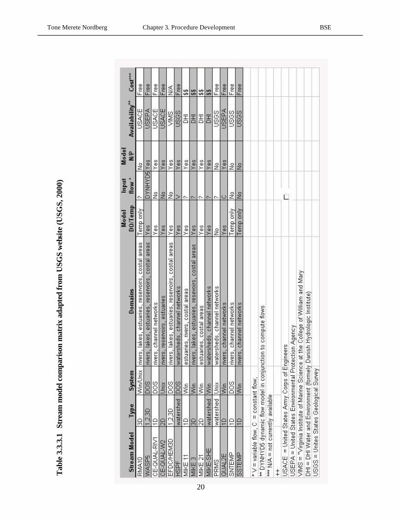
the stream model as input to the stream. In table 3.3.3.1 are the models that were considered and
compared. WASP5 from EPA was not available for download when the model selection was
done, hence it could not be evaluated in detail.
From Table 3.3.3.1, QUAL2E, HSPF and the MIKE models were the only ones that met all
requirements. The MIKE models were ruled out due to the cost of obtaining the models
compared to QUAL2E and HSPF being free of cost. In addition, DHI Water and Environment
owns the MIKE models and must approve their use. QUAL2E first appeared to be more
appropriate than HSPF because QUAL2E has a more detailed water chemistry routine and is a
stream only model. QUAL2E applies a finite-difference solution to the advective-dispersive
mass transport and reaction equations and simulates up to 15 water quality constituents in a
channel network. Differential equations are applied to calculate P and DO concentrations in the
stream network. Because QUAL2E has what is termed a “dynamic” mode, it was thought that
hydrographs could be input to the model. Further investigation showed that QUAL2E is a
constant flow model with a dynamic weather component. Therefore, hydrographs from
ANSWERS-2000 could not be input into the stream via QUAL2E. In addition, the maximum
length of simulation for QUAL2E was less than 900 hours, not long enough to generate the
required sample size. HSPF can accept variable inflow of both hydrographs and pollutographs
and infinite simulation length. Though its methods are less detailed than QUAL2E, HSPF can
model a wide variety of water quality constituents, sediment and nutrients, including DO and P
balances and concentrations. Thus, HSPF met all criteria for the stream model.
Tone Merete Nordberg Chapter 3. Procedure Development BSE
20
Tab
le 3
.3.3
.1
Stre
am m
odel
com
pari
son
mat
rix
adap
ted
from
USG
S w
ebsi
te (
USG
S, 2
000)

Tone Merete Nordberg Chapter 3. Procedure Development BSE
21
Hydrological Simulation Program FORTRAN (HSPF) is a mathematical model developed in the
late 1970’s and early 1980’s (Singh, 1995) to simulate hydrologic and water quality processes in
natural and constructed water systems. It is a somewhat distributed watershed model that
simulates precipitation and snowmelt movement through the watershed by modeling overland
flow, interflow, and baseflow. Kinematic routing of one-dimensional flow, in the direction of
flow, is also included. Receiving channel networks are assumed to be well-mixed systems. The
time scale of the model can be user-defined to handle a single event or long-term modeling over
a period of 50 to 100 years.
Only the channel network part of HSPF, the module called RCHRES, was used since the
overland flow modeling was done in ANSWERS-2000. The RCHRES module simulates water
quality processes and flows in a single reach of an open or closed channel or a completely mixed
reservoir. The different reaches are joined with a network module. The flow in each reach is
unidirectional with a single inlet but possible multiple outlets. Sediment detachment, transport
and scouring can be considered in the model, but assumed not to affect the hydraulic properties
of the channel. The oxygen subroutine considers longitudinal advection of DO and biochemical
oxygen demand (BOD), benthal oxygen demand and release of BOD materials, sinking of BOD
material, reaeration and oxygen depletion caused by decay of BOD material. The subroutine has
three options for calculating the oxygen reaeration coefficient in the stream. The nutrient
subroutine simulates the basic processes that determine the balance of N and P in a water system,
and if the plankton subroutine is active, it also accounts for N and P consumed by plankton
populations.
3.3.4 Weather Data Preparation
ANSWERS-2000 can use generated or measured weather data. For the risk quantification
procedure, statistical weather data generated with CLIGEN was chosen. CLIGEN is a statistical
weather data generator originally written for EPIC and later modified for WEPP (Nicks et al.,
1995). CLIGEN uses a two-state Markov chain for generating number and distribution of
precipitation events. The Markov chain calculates two conditional probabilities, i.e., α, the

Tone Merete Nordberg Chapter 3. Procedure Development BSE
22
probability of a wet day given the previous day was dry, and β , the probability of a dry day
following a wet day (Nicks et al., 1995):
P (W | D) = α [3.3.4.1]
P (D | D) = 1-α [3.3.4.2]
P (D | W) = β [3.3.4.3]
P (W | W) = 1-β [3.3.4.4]
Where: P(W|D) = probability of a wet day given a dry day;
P(D|D) = probability of a dry day given a dry day;
P(D|W) = probability of a dry day given a wet day; and
P(W|W) = probability of a wet day given a wet day.
Then CLIGEN uses a skewed normal distribution to estimate the daily precipitation amounts for
each month. Based on the Markov chain conditional probabilities and the distribution of daily
precipitation amount, the total rainfall for each day is computed.
Using a statistical weather generator has advantages in that any desired length of run can be done
without having to consider available historic records. It is also possible to generate as many
weather data files as desired for the same period of time with different rainfall. In the developed
procedure, stochastic variability in weather was the main factor in risk quantification, hence the
length of simulation was very important. A length of record long enough to capture the stochastic
variability of weather was considered important to ensure a accurate representation of the
stochastic uncertainty. In addition the sequence of the weather record was important, since this
could greatly skew the results. ANSWERS-2000 is a continuous model, hence a storm event in
days prior to a storm will affect the runoff volume and duration for the storm. The number of
days in between rainfall events and number of continuous precipitation days will affect the
output of the model. Each storm event is not an independent event in a continuous model like
ANSWERS-2000.

Tone Merete Nordberg Chapter 3. Procedure Development BSE
23
To determine the length of simulation required to obtain a sample of adequate size for
distribution fitting, two methods were used. For both methods, three 100-year data sets were
generated from CLIGEN. The first data set was generated with the first seed in CLIGEN, which
is constant, and the two other data sets were generated with random seeds. For the first method, a
two-sided t-test assuming unequal variances was performed on each data set comparing annual
precipitation amounts. Lengths of 100-years to 50-years, 100-years to 25-years and 100-years to
10-years were compared. The second method involved an iterative process of comparing the
monthly means for the three data sets. The total rainfall amounts for each individual month were
separated into twelve record sets starting with the first year. As each consecutive year was added
to the record set, the mean and standard deviation were calculated and compared to those of the
previous iteration. Years were added to the record set until the mean and standard deviation did
not change significantly indicating that an adequate length of record was found. The results of
both the monthly mean comparison and the annual average comparison were used to determine
the length of record that would give an adequate sample size. The results will vary depending
upon the weather station data used; hence this evaluation had to be conducted for the specific
area being modeled. The longer of the two length of records suggested adequate by the two sided
t-test performed on the annual precipitation amounts and the mean monthly comparison was
used.
The required weather input to ANSWERS-2000 includes precipitation, soil and air temperature,
and total daily solar radiation. The precipitation must be entered in a hyetograph format with a
maximum of 11 entries with the units of mm/hr. CLIGEN outputs total precipitation, duration of
precipitation and maximum intensity. Based on this information a breakpoint data program,
which comes with QUESTIONS, uses a SCS triangular hydrograph approach to make the
hyetograph for ANSWERS-2000. The CLIGEN output format limits the number of storms per
day to one. Since ANSWERS-2000 only allows for a maximum of 11 entries in the daily
hyetograph, longer duration storms are not represented with the same resolution as shorter
storms.
The in-stream modeling done with HSPF required different weather inputs and formats than
ANSWERS-2000. HSPF reads weather data management files (WDM-files), which are binary

Tone Merete Nordberg Chapter 3. Procedure Development BSE
24
data files containing the time series data needed depending on which parts of HSPF are being
used. WDMUtil, a free program distributed and maintained by USEPA, was used to create and
edit the WDM file for HSPF input. Raw data needed to create the WDM file included daily
minimum and maximum temperature (ºF), daily average dew-point temperature (º F), total daily
solar radiation (ly/day), daily cloud cover in tenths and total daily wind speed (mi/day). For the
in-stream modeling, the precipitation that falls directly into the stream was ignored and no
precipitation data were entered into HSPF. All the required inputs for HSPF were included in
the CLIGEN output file except cloud cover. The CLIGEN output file was opened in EXCEL and
processed so every parameter was saved as a separate time series text file with one column for
date (mm/dd/yyyy) and one column with the corresponding parameter value. To read the created
text files into WDMUtil, ASCII formatting was used (m2,x,d2,x,y4,f9,v8).
The daily maximum (TMAX-F) and minimum (TMIN-F) temperature data were used to
calculate hourly air temperatures (FTEM) using the DISAGGREGATE function in the
WDMUtil program. The average daily dew-point temperature (FDEW) was disaggregated with
the same function to produce hourly dew-point temperatures (DEWP). Total daily solar radiation
(DSOL) and total daily wind speed (DWIND) were read into WDMUtil and then disaggregated
with the DISAGREGATE function into hourly values (SOLR) and (WIND), respectively.
In WDMUtil, the following time series were calculated. Daily maximum and minimum
temperatures (TMAX and TMIN) were used to calculate daily evapotranspiration (DEVT,
in/day) by the Harmon method. Daily evapotranspiration was disaggregated with the
DISAGGREGATE function to hourly values (PEVT, in/hr). Daily pan evaporation (DEVP) was
calculated from daily maximum (TMAX-F) and minimum (TMIN-F) temperatures, daily dew-
point temperature (TDEW-F), daily wind speed (DWIND-F) and daily solar radiation (DSOL).
Finally, daily pan evaporation was disaggregated to hourly values (EVAP) with the
DISAGGREGATE function for evapotranspiration, as WDMUtil does not have a disaggregate
function for evaporation.
Tone Merete Nordberg Chapter 3. Procedure Development BSE
25
Daily cloud cover was not given in the CLIGEN output. A relationship between observed solar
radiation and extraterrestrial solar radiation that involved the ratio between actual and possible
hours of sunshine, n/N, was used (James, 1988):
Rs = (0.25+0.50n/N)Ra [3.3.4.5]
Where: Rs = extraterrestrial solar radiation (mm/day);
Ra = observed solar radiation in evaporation equivalents (mm/day); and
n/N = ratio between actual and possible hours of sunshine.
Cloud cover was estimated as (1-n/N). Daily observed solar radiation, an output from CLIGEN
in langleys/day, was converted to mm/day by assuming a heat of vaporization of 585 cal/g.
Extraterrestrial solar radiation was calculated from the radius vector of the earth, the declination
of the sun, latitude of location and Julian day of the year. The spreadsheet used to calculate cloud
cover is included in Appendix A.
The CLIGEN weather dataset used for ANSWERS-2000 ran from 01/01/2000 to 12/31/2049,
which are arbitrary values since the data were generated. WDMUtil was written primarily to
manipulate historic datasets and does not allow for entries beyond year 2020. This restriction
would not allow for an HSPF simulation from 01/01/2000 to 12/31/2049. The initial solution of
shifting the HSPF run 100 years back in time to 1900 to 1949 proved difficult since year 2000 is
a leap year while year 1900 is not a leap year. The definition of a leap year introduced with the
Gregorian calendar by Pope Gregory XIII in 1582 states that every fourth year is a leap year
except centuries that are not divisible by 400, thus making the year 2000 a leap year and 1900
not a leap year (The Royal Observatory Greenwich, 2000). Hence the HSPF run was shifted back
to a start date of 01/01/1940 and end date of 12/31/1989 to match the leap years. This problem
could have easily been avoided if the restriction on WDMUtil had been known prior to
completing the ANSWERS-2000 simulations.

Tone Merete Nordberg Chapter 3. Procedure Development BSE
26
3.3.5 ANSWERS-2000 Modeling
ANSWERS-2000 produces best results on smaller watersheds with the majority of flow being
overland flow. In addition, ANSWERS-2000 only produces hydrographs and pollutographs at
the watershed outlet point. With this in mind, for this procedure a watershed should be divided
into subwatersheds, resulting in an individual ANSWERS-2000 simulation for each
subwatershed that has an outlet to the main stream. The main stream can be defined based upon
visual inspection of topographic maps. By dividing the watershed into subwatersheds, the NPS
pollutant loading from each subwatershed can be identified and the resultant environmental risk
imposed on the system due to the pollutant loadings can be estimated.
The following steps which are performed for each of the subwatersheds are automated by
QUESTIONS. The first step involves filling sinks in the Digital Elevation Model (DEM) of the
watershed. Sinks may be natural sinkholes or sinks created as a result of data entry error, but
they cannot be present on the map when the watershed boundaries are generated by ArcView.
Next, grid layers are generated for each of the following: flow direction, flow accumulation,
aspect, slope, stream network, watershed boundary, and drop in direction of stream flow.
ANSWERS-2000 requires streams to be grouped according to equal characteristics.
QUESTIONS does this by assuming a Strahler (e.g. Chow et al., 1988) ordering scheme. After
all the hydrology grids are created, the landuse and soils maps are cut to match the watershed
area defined by the hydrologic grids. Subwatersheds located completely downstream of other
subwatersheds create a problem in defining the watershed since ArcView automatically defines
everything upstream of a point as part of the watershed. To prepare the ANSWERS-2000 input
files for such watershed files, QUESTIONS is used to generate the upstream areas. Then the
upstream areas are manually removed using the Spatial Analyst extension package to ArcView.
3.3.6. From ANSWERS-2000 Output to HSPF Input
Running two different models in sequence with the output from one as the input to the other
most often presents challenges as the input format and requirements are different and seldom
does a model output exactly what the next model needs as input. ANSWERS-2000 and HSPF

Tone Merete Nordberg Chapter 3. Procedure Development BSE
27
were no exception, though the sequential running proved to be less difficult than first anticipated.
Two main differences in ANSWERS-2000 output and HSPF input had to be dealt with. HSPF
and ANSWERS-2000 both require sediment particle classes, but ANSWERS-2000 does not
output sediment delivery in different particle size classes. Second, ANSWERS-2000 outputs
hydrographs and pollutographs in a file separated by a line stating the date of the storm, while
HSPF requires a continuous constant time step input. These two problems were solved as
follows.
HSPF requires that sediment and sediment-bound nutrients be loaded in terms of sand, silt and
clay particle classes. While particle class distribution is an input to ANSWERS-2000, sediment
loss is output as a total for all particle sizes. To address this, one array for sediment, one for
nitrogen and one for phosphorus were added to the loop in ANSWERS-2000 that sums the
sediment particle size classes. These three arrays were then summed by particle class and
averaged over the simulation period to provide the required input to HSPF.
ANSWERS-2000 hydrograph and pollutograph output are written to one file for the length of
simulation, where hydrographs and pollutographs for each storm are separated with a line stating
the date of the storm. HSPF requires a continuous time series input including the intermittent
periods between storms in an input file called Multiple Sequential Input of Time Series
(MUTSIN). A Visual Basic (VB) program called HplotEnglish was written to handle the
conversion of such a large volume of data for each subwatershed from ANSWERS-2000 into
HSPF. The code for this program is included in Appendix B. The output of HplotEnglish was a
MUTSIN file for each subwatershed that contained flow, sediment, sediment-bound P, dissolved
P, sediment-bound NH4+, and dissolved NO3
- time series for the simulation period.
3.3.7 HSPF Modeling
The hydrographs and pollutographs from the subwatersheds run in ANSWERS-2000 were
loaded into HSPF. The main input file for HSPF, the Users Control Input (UCI) file, can be
written in a text editor. Several programs are available to assist in input file construction, but

Tone Merete Nordberg Chapter 3. Procedure Development BSE
28
since only the RCHRES module was used, it was relatively straightforward to write the file in a
text editor with aid from the HSPF documentation.
Initially, input data for HSPF were prepared in SI units. However, the model calculations were
incorrect; it appeared that HSPF did not read the MUTSIN files properly in SI units. Using
English units in HSPF meant converting all outputs from ANSWERS-2000 from SI units.
3.3.8 Risk Quantification
After both ANSWERS-2000 and HSPF simulations are completed, the final steps of combining
the results and calculating the watershed risk are performed. A flow chart of the complete
procedure is shown in Figure 3.3.8.1.
Figure 3.3.8.1: Schematic of risk quantification procedure

Tone Merete Nordberg Chapter 3. Procedure Development BSE
29
To generate the best-fit distribution for the pollutant loadings, the loadings from all
subwatersheds are first added together to produce a total pollutant loading for every hour in the
watershed. The subwatershed total pollutant loadings were flow-weighted to give total pollutant
loadings in mg/L. Due to the large amount of data, a VB program called MutReader was written
to automate this process. The code is included in Appendix C. ExpertFit (Averill Law), a
statistical software package that fits data to the best fit distributions from a selection of more than
twenty of the most common distributions, was used to fit a distribution to the pollutant loading
data set output from the MutReader program. ExpertFit can fit an empirical distribution to the
data in the event that none of the models included in ExpertFit gives a good fit. The empirical
distribution is based on the unique observations in the data set. The unique observations in the
data set, Y[1], Y[2], Y[3],….,Y[m] are arranged in increasing order. If all observations in the
sample are unique, the sample size n equals the number of different observations, m. The
empirical function is then fitted based on the following equation:
[3.3.8.1]
Where: Y[i] = value in sample set of interest; and
n = total number of observations in data set.
The final step in the procedure is to calculate the risk as the product of the probability of
occurrence of the event of interest and the consequences of that event, where the event of interest
is pollutant loading to surface waters. The output from HSPF is read into a third VB program,
called RiskCalc, together with the watershed pollutant loadings from the MutReader program.
Figure 3.3.8.2 shows how the two data sets were linked together.
[ ] [ ]1
1#−
−≤=
niYsamples
iY

Tone Merete Nordberg Chapter 3. Procedure Development BSE
30
Figure 3.3.8.2: Schematic of linking ANSWERS-2000 output to HSPF output
The RiskCalc program was partly written for the specific endpoint selected for the application of
the risk quantification procedure, which has to be specifically defined for each application. The
source code for the RiskCalc program is included in Appendix D. RiskCalc reads in the total
pollutant loading from the watershed for every hour and the output file from HSPF containing
the time, flow, and selected environmental point for every hour. Then the second part of the
program takes the following input; criterion for which the case specific endpoint is measured,
total pollutant loading for each hour and the probability of exceeding that pollutant loading. The
actual risk equation will vary depending on the endpoint selection. To illustrate the procedure, a
total phosphorus (TP) loading impact on DO could be written as:
[ ]i
i xTPhoursStdDOhours
xTPPRisk><×>=
_#._# [3.3.8.2]
Where: Risk = risk of DO below standard;
TP = total pollutant loading, expressed as a flow-weighted concentration, from
watershed, mg/L;
xi = the loading of interest, mg/L; and
DO = dissolved oxygen concentration, mg/L.
Resulting from this equation is a risk level expressed in number of hours the DO dropped below
standard divided by the total number of hours that the TP loading was in the given range. This

Tone Merete Nordberg Chapter 3. Procedure Development BSE
31
results in a dimensionless number between 0-1, where 1 represents a 100% chance of DO
dropping below standard when the specified loading is exceeded.
From a watershed management perspective, the total pollutant loading as a loading per hour
might be of equal importance as the total pollutant concentration. The concentration has the
advantage of being flow-weighted, but from a management point of view, the allowable pollutant
loading might be a more useful value in the daily management of the watershed.
3.4 Summary of Procedure Implementation
The risk quantification procedure, as implemented, involves the following steps:
• Identify the pollutant loading and environmental endpoint of interest.
• Formulate the risk quantification equation specific for the pollutant loading and
environmental endpoint of interest.
• Obtain necessary data for the watershed, including DEM, landuse and soils data.
• Calculate fertilizer application requirements according to landuse and soils.
• Locate weather station to use and identify the length of record needed for the simulation
based on both annual and monthly averages of precipitation.
• Use ANSWERS-2000 to estimate upland pollutant loading.
• Use HSPF to estimate upland pollutant loading impact on receiving water.
• Fit the pollutant loading data to a distribution using ExpertFit.
• Calculate the watershed risk with the RiskCalc program using the output from HSPF and
probability distribution from ExpertFit.
At this time ANSWERS-2000 does not model impervious areas adequately, hence the risk
quantification procedure, as implemented here, should be applied to mainly agricultural
watersheds for the best result.
Tone Merete Nordberg Chapter 4. Application of procedure BSE
32
4.0 Application of Procedure
4.1 Introduction
To illustrate the developed procedure, a watershed with readily available data was needed. The
data needed for the procedure includes a DEM covering the watershed area, landuse for the
watershed and soils data in Soil Survey Geographic (SSURGO) data from USDA-Natural
Resources Conservation Service (NRCS, 2000) compatible format. In addition, a watershed with
relatively intense agricultural activity would better demonstrate the use of the procedure since
ANSWERS-2000 does not simulate urbanized, impervious areas adequately at this time. Total
phosphorus (TP) was selected as the pollutant of interest and dissolved oxygen (DO) was
selected as the endpoint of interest. The risk procedure as described in the previous chapter was
applied to the watershed and the risk of DO dropping below the state water quality standard for
DO at the watershed outlet as a result of TP loading in the watershed was investigated. Although
economic consequences and cost were beyond the scope of this project and therefore not
considered, economic factors certainly should be considered in performing a risk analysis for a
watershed. A management strategy proposed by conducting a risk analysis cannot be
implemented without considering economic implications for the inhabitants in the watershed.
In applying the risk quantification procedure to a watershed, SI units were used as far as
possible, but some English units also had to be incorporated in running HSPF. In reporting
numbers the SI units are given with the English units in parentheses.
4.2 Test Watershed Selection
The Muddy Creek watershed in Rockingham County was selected for demonstrating the
application of the risk quantification procedure. The Muddy Creek watershed is located in
Virginia’s most agriculturally intensive area with high livestock and poultry production per land
area unit. The watershed has been the subject of several previous studies. As a result, the
required data were readily available.

Tone Merete Nordberg Chapter 4. Application of procedure BSE
33
Muddy Creek watershed has a total area of about 8184.8 ha (20225 acres). When a grid layer
with 30 by 30m cells, which is the resolution of USGS DEMs, was overlaid on the watershed,
the number of cells exceeded the maximum of 35000 cells allowed in ANSWERS-2000. As a
result, a subwatershed within the Muddy Creek watershed was selected. The stream in the
selected subwatershed is not named, therefore, for convenience, it was named Lola Run for the
purpose this thesis. Figure 4.2.1 shows the location of the Lola Run subwatershed within the
Muddy Creek watershed.
Figure 4.2.1: Location of Lola Run watershed within Muddy Creek watershed
Lola Run enters Muddy Creek at Mount Clinton water quality station. It is marked as a dashed
blue line stream on USGS topographic maps, indicating it will go dry in droughts and long
periods without rainfall. Photographs taken on December 19, 2000 of Lola Run, the side bank,
conditions around the stream and the junction where Lola Run enters Muddy Creek are shown
in figures 4.2.2 through 4.2.5.
De m-org377 - 454455 - 531532 - 609610 - 686687 - 763764 - 841842 - 918919 - 995996 - 107 3No Da ta
Stream Network (10 0)Lola R un W a te rshe d
4 0 4 8 Mi les
N
EW
S
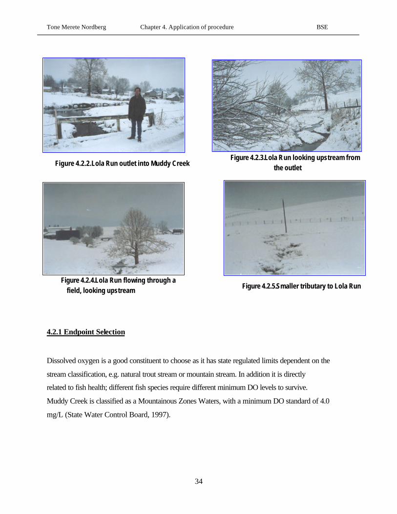
Tone Merete Nordberg Chapter 4. Application of procedure BSE
34
4.2.1 Endpoint Selection
Dissolved oxygen is a good constituent to choose as it has state regulated limits dependent on the
stream classification, e.g. natural trout stream or mountain stream. In addition it is directly
related to fish health; different fish species require different minimum DO levels to survive.
Muddy Creek is classified as a Mountainous Zones Waters, with a minimum DO standard of 4.0
mg/L (State Water Control Board, 1997).
Figure 4.2.2.Lola Run outlet into Muddy Creek Figure 4.2.3.Lola Run looking upstream from the outlet
Figure 4.2.4.Lola Run flowing through a field, looking upstream Figure 4.2.5.Smaller tributary to Lola Run

Tone Merete Nordberg Chapter 4. Application of procedure BSE
35
4.3 Lola Run Landuse
The landuse in the Lola Run watershed (figure 4.3.1) was obtained from the Virginia Department
of Conservation and Recreation (VDCR). Field boundaries were determined using 1990
Rockingham County DOQQ orthophotographs, classified landuses from 1989 and 1991 National
Aerial Photography Program (NAPP) and 1992 and 1994 Farm Service Agency (FSA) aerial
slides (Heatwole, 1999).
Figure 4.3.1. Landuse in Lola Run watershed
Five landuse categories were identified for Lola Run. The “other” category included
farmsteads, loafing lots, poultry houses and rural residential buildings. In table 4.3.1, the
landuse categories are listed with the corresponding areas.
La nduse-Lola R uncroplandfores t_orc hha yotherpa sture1 0 1 2 Mi le s
N
EW
S

Tone Merete Nordberg Chapter 4. Application of procedure BSE
36
Table 4.3.1 Lola Run landuse categories and areas
Landuse Description # fields in
landuse category
Total area
ha (acres)
% of total
watershed area
cropland 60 394.1 (973.9) 38.9
forest orchard n/a 188.5 (465.7) 18.6
hay 33 282.6 (698.2) 27.9
pasture 11 94.1 (232.5) 9.3
other n/a 53.9 (133.3) 5.3
The total watershed area is 1013.2 ha (2503.6 ac), of which 53.9 ha (133.3 ac) is classified as
“other”. The other category makes up just over 5% of the total watershed area. In running
ANSWERS-2000, these areas were merged with the spatially closest field to avoid having
impervious areas.
A commonly used crop rotation in the Muddy Creek watershed is corn silage rotated with rye
cover or rye silage. Hence this rotation was assumed on all cropland for the modeling. In
addition alfalfa hay and pasture are common in the area. Table 4.3.2 shows the detailed outline
of the landuse management.
Table 4.3.2 Landuse and management practices for Lola Run used in ANSWERS-2000
Landuse Management Fertilizer application
Cropland Corn silage w/ winter rye
grain
Fertilized according to Virginia VALUES*
recommendations for soil type
Hay Alfalfa hay Fertilized according to Virginia VALUES
recommendations for soil type
Pasture Native permanent pasture Fertilized according to Virginia VALUES
recommendations for soil type
Forest /
Orchard
Forest (good standing) No fertilizer applied
* VALUES refers to the Virginia Agronomic Land Use Evaluation System. It is a database
developed at Virginia Polytechnic Institute and State University to base fertilizer application on
crop grown, soil type, and expected yield (Simpson et al., 1992).

Tone Merete Nordberg Chapter 4. Application of procedure BSE
37
4.4 Lola Run Soils
The soils data set obtained for Lola Run watershed (Figure 4.4.1) was Soil Survey Geographic
(SSURGO) data from USDA-Natural Resources Conservation Service (NRCS, 2000). The
SSURGO data are the most detailed soils maps produced by the NRCS. The field mapping
methods used in producing the maps follow national standards. The SSURGO maps are available
for download by county on the NRCS World Wide Web page
(http://www.ftw.nrcs.usda.gov/ssur_data.html). Certain soils in the database were identified on
the digitized map but did not have any attributes in the attributes table. In these cases, a
neighboring soil, either based on similar soil properties or majority area, was substituted.
Figure 4.4.1: Lola Run soils map (NRCS, 2000)
Soil s in Lola RunAll egheny cobbly fine s andy l oa mAll egheny fine s andy loamAquic Udifluvev ents near ly l eve lBe rks -W e ike rt Sha ly s ilt loa mBucha na n cobbly fine s andy l oamDra ll e x tre mel yEndc a v s lit loa mFluvaque nts nea rly le velFre de ric k and Lodi c he rty si lt loamsFre de ric k and Lodi s il t loamFre de ric k and Lodi s il t loam r oc kyFre de ric k rock outcrop c om pl e xGuerne sy s i lt loamLaidig c obbl y fine sa ndy loa mLaidig gr ave lly fine s andy loamLaidig v ery stony fine s andy l oa mMonogahe la f ine s andy loa mPurdy s il t l oam (drai ned)Rock Outc rop lai di g Comple xRock and outc rop Fre deric k c omple xSe quoia -Be rk s si lt loamShenv al Loa mTim berv ille Va ria nt s ilt l oamWe ika rt-Be rk s ve ry s tony sil t loa m
1 0 1 2 Miles
N
EW
S
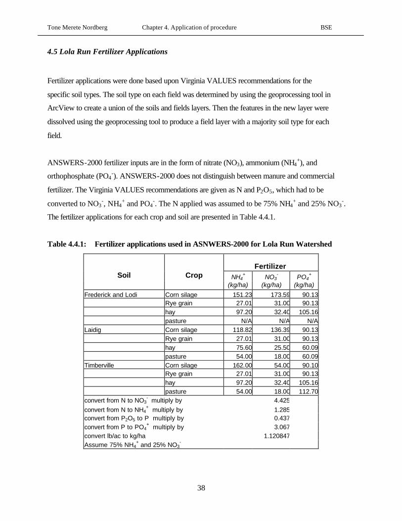
Tone Merete Nordberg Chapter 4. Application of procedure BSE
38
4.5 Lola Run Fertilizer Applications
Fertilizer applications were done based upon Virginia VALUES recommendations for the
specific soil types. The soil type on each field was determined by using the geoprocessing tool in
ArcView to create a union of the soils and fields layers. Then the features in the new layer were
dissolved using the geoprocessing tool to produce a field layer with a majority soil type for each
field.
ANSWERS-2000 fertilizer inputs are in the form of nitrate (NO3), ammonium (NH4+), and
orthophosphate (PO4-). ANSWERS-2000 does not distinguish between manure and commercial
fertilizer. The Virginia VALUES recommendations are given as N and P2O5, which had to be
converted to NO3-, NH4
+ and PO4-. The N applied was assumed to be 75% NH4
+ and 25% NO3-.
The fertilizer applications for each crop and soil are presented in Table 4.4.1.
Table 4.4.1: Fertilizer applications used in ASNWERS-2000 for Lola Run Watershed
Fertilizer
Soil
Crop
NH4+
(kg/ha) NO3
-
(kg/ha) PO4
+
(kg/ha)
Frederick and Lodi Corn silage 151.23 173.59 90.13 Rye grain 27.01 31.00 90.13 hay 97.20 32.40 105.16 pasture N/A N/A N/ALaidig Corn silage 118.82 136.39 90.13 Rye grain 27.01 31.00 90.13 hay 75.60 25.50 60.09 pasture 54.00 18.00 60.09Timberville Corn silage 162.00 54.00 90.10 Rye grain 27.01 31.00 90.13 hay 97.20 32.40 105.16 pasture 54.00 18.00 112.70convert from N to NO3
- multiply by 4.425 convert from N to NH4
+ multiply by 1.285 convert from P2O5 to P multiply by 0.437 convert from P to PO4
+ multiply by 3.067 convert lb/ac to kg/ha 1.120847 Assume 75% NH4
+ and 25% NO3-

Tone Merete Nordberg Chapter 4. Application of procedure BSE
39
4.5 Weather Data
CLIGEN uses distributions based on historical data to generate a statistical weather file. The user
must select a weather station with historical records in CLIGEN. In this case, Big Meadows
weather station in Madison County, approximately 56.3 km (35 miles) east of Lola Run, was the
closest location. To do a comparison of annual averages in the first seed compared to the
following random seeds in CLIGEN, three datasets of 100 years of data were generated from
CLIGEN. The first set was generated with the first seed, which is constant, and the second and
third sets with random seeds. Total annual rainfall was very similar in the three data sets, about
1240 mm per year (48.8 in/year). To determine the length of simulation needed so that an
extreme year in either direction would not significantly change the mean, a two-sided t-test
assuming unequal variances was used on the annual total precipitation.
Table 4.5.1: Two sided t-test of annual rainfall at Big Meadows weather station
P-values from two sided t-test on 3 sets of weather data from CLIGEN
H0: µµ = µµ 0 ; H1: µµ ≠≠ µµ 0
Seed selection 100 years to 50 years 100 years to 25 years 100 years to 10 years
1st seed 0.550 0.033 0.099
Random seed 1 0.773 0.632 0.942
Random seed 2 0.662 0.226 0.732
The results (table 4.5.1) suggested that the selection of an appropriate weather data set was not
sensitive to the total annual rainfall. The only time the null hypothesis could be rejected for a
significance level of 0.05 was for the first seed comparing 100 years to 25 years (p-value=0.033).
If the significance level was increased to 0.1 the null hypothesis for the first seed 100 years to 25
years and 100 years to 10 years were both rejected. For two of the three seeds, a 10-year set was
not statistically different from a 100-year set.
The monthly mean precipitation amounts were summed in an iterative process, comparing every
new iteration to the previous iteration for 50 years of statistical generated data. The results of the

Tone Merete Nordberg Chapter 4. Application of procedure BSE
40
mean precipitation comparison for December for the 50 years from three different data sets are
shown in Table 4.5.2.
Table 4.5.2: Mean monthly precipitation for December for 50 years of data
Observed mean precipitation for December at Big Meadows = 92.7 mm
Seed Selection Mean Precipitation Standard Deviation
1st seed 90.5 mm (3.56 in) 72.6 mm (2.86 in)
Random seed 1 79.3 mm (3,12 in) 47.1 mm (1.85 in)
Random seed 2 81.2 mm (3.20 in) 59.0 mm (2.32 in)
It was found that a length of record of 50 years was required before an extreme value in either
direction would have no significant impact on the monthly means. Hence for the final dataset,
the second random seed in CLIGEN was used with a length of simulation of 50 years. Figure
4.5.1 shows the annual rainfall amounts for the weather data set used, and the observed annual
average reported at the Harrisonburg NRCS office. The annual rainfall amount for the weather
data set used had a mean of 1237 mm (48.7 in) compared to the observed 853.2 mm/year (33.6
in/year) rainfall at Dale Enterprise weather station also located in the Shenandoah Valley just
south of Harrisonburg (http://climate.virginia.edu/Climate/normals/442208_30yr_norm.html).
This difference was expected since the Big Meadows weather station is on the east side of the
Blue Ridge Mountains and Lola Run is on the west side. Big Meadows however is the closest
located weather station in CLIGEN and was considered adequate for demonstrating the risk
quantification procedure.

Tone Merete Nordberg Chapter 4. Application of procedure BSE
41
Figure 4.5.1: Generated annual rainfall data set used in ANSWERS-2000 compared to observed annual average
4.6 ANSWERS-2000 Modeling of Lola Run
Lola Run was divided into twelve subwatersheds (Figure 4.6.1) using the watershed calculate
function in the Map Calculator in ArcView. The watershed was divided into subwatersheds to
create pollutant loading points in the main stream, which could be input points to the stream
modeled in HSPF. Due to the output format and options of ANSWERS-2000, the pollutant
loading points were best created by modeling several smaller subwatersheds with the outlet point
of each subwatershed entering the main stream. The total number of subwatersheds was
determined so that every subwatershed discharged into the main stream modeled in HSPF.
600
800
1000
1200
1400
1600
1800
2000 2005 2010 2015 2020 2025 2030 2035 2040 2045 2050
time, years
rain
fall,
mm
PRECIP MM
Observed annual avg. Dale Enterpriser

Tone Merete Nordberg Chapter 4. Application of procedure BSE
42
Figure 4.6.1: Subwatershed division of Lola Run watershed
For each of the twelve subwatersheds, QUESTIONS was used to generate the ANSWERS-2000
input files. In addition to the GIS data, the parameters required to characterize the cover, tillage
and residues of the different landuses were generated from the database included in
QUESTIONS. ANSWERS-2000 was run for each subwatershed separately. ANSWERS-2000
produces an output file with sediment and nutrient losses from each cell. These data were
imported into ArcView using QUESTIONS to give a spatial representation of the output.
Sediment loss and dissolved PO4- output from watershed 2 are displayed in figures 4.6.2 and
4.6.3, respectively. A complete set of results for all subwatersheds is presented in Appendix E.
The ANSWERS-2000 cell by cell output when imported back into ArcView illustrates the
location in the watershed with higher sediment and pollutant loadings. From a watershed
management standpoint, this output can be used to identify where to implement best
management practices (BMPs) to best reduce the overall risk level in the watershed. All twelve
subwatersheds followed the same general trends, with a few fields in each watershed producing
2
9
4
6
1
12
8
5
10
3
7
11
0.5 0 0.5 Miles
Lola Run Subwate rsheds123456789101112
Drainage networkLol a-run
N
EW
S

Tone Merete Nordberg Chapter 4. Application of procedure BSE
43
the majority of the sediment and nutrient loadings. Sediment and nutrient losses were higher on
cropland than pasture, which was expected. Sediment loss was higher in watershed areas with
cropland on steeper slopes, which was also expected.
Figure 4.6.2: Average annual sediment loss output from ANSWERS-2000 for Subwatershed 2. A positive number indicates a net sediment deposit and a negative number indicates a net sediment loss from the cell.
Sediment loss, kg/ha-120966 - -103962-103962 - -86958-86958 - -69953-69953 - -52949-52949 - -35945-35945 - -18941-18941 - -1936-1936 - 00 - 3207232072 - 4907649076 - 6608066080 - 8308483084 - 100088100088 - 117093117093 - 134097134097 - 151101No Data
Landusecroplandforest_orch
haypasture
Stream
0.6 0 0.6 Miles
N
EW
S

Tone Merete Nordberg Chapter 4. Application of procedure BSE
44
Figure 4.6.3: Dissolved PO4 output from ANSWERS-2000 for Subwatershed 2 in total phosphorus
loss in kg/year
4.7 HSPF Modeling
The HSPF model was used only for the stream modeling, which meant that most of the inputs
were outputs from ANSWERS-2000 that were transformed using the HplotEnglish program.
HSPF requires stage discharge relationships (F-tables) as part of the input. These were developed
assuming a trapezoidal channel cross-section with the first meter (3.28 ft) having a side slope of
1:2; beyond 1m the side slopes were assumed to be 1:5. The bottom width of the channel was
measured to be about 2.5 m (8.2 ft) to 3 m (9.8 ft) at the outlet point, with gradual narrowing
moving upstream. Details of the F-tables calculations are included in Appendix F.
To estimate an appropriate time step for use in HSPF, a travel time calculation was performed
for the shortest reach in the reach network. To calculate the velocity in the reach, normal depth
was assumed. Normal depth is the depth of uniform flow under constant discharge. The length of
the shortest reach was 1410 ft and the maximum flow during a storm was 410 cfs, resulting in a
Diss olved PO4, kg0 - 55 - 1010 - 1515 - 2020 - 2525 - 5050 - 100100 - 125125 - 150150 - 175175 - 200No Data
Landusecroplandforest_ orc h
haypasture
Stream
0.6 0 0.6 Miles
N
EW
S
Tone Merete Nordberg Chapter 4. Application of procedure BSE
45
velocity of 5.0 ft/sec and a travel time through the reach of 4.7 min. The 410 cfs storm was the
largest runoff event produced in ANSWERS-2000. For travel time calculations see Appendix G.
Based on this calculation the time step in HSPF was set to 4 minutes. The printout time step was
set at 1-hour and an average of the 4-minute interval values was printed.
HSPF relates P loading to DO concentration through phytoplankton and zooplankton
consumption of nutrients in the system. The P uptake increases production in the waterbody
which results in increased DO consumption by the planktons. The increased DO consumption
lowers the available DO in the waterbody.
A few storms were selected and mass balances of flow and sediment were performed to check
the model performance. The storm occurring on February 2, 2000 (year 1940 in HSPF) with a
total rainfall of 37.3 mm over a 7 hour period had a total inflow of 39101.4 m3 (31.7 ac-ft) and
an outflow of 38978.0 m3 (31.6 ac-ft). The sediment balance for the same storm gave a total
inflow of 25129 kg (55400 lb) and outflow of 20321 kg (44800 lb). The slight reduction in
sediment outflow compared to inflow is due to sediment deposition in the channel. The stream in
HSPF was modeled to allow for sediment deposition and detachment of previous deposited
sediment. The channel erodibility factor was set to 0.0, meaning no channel scouring was
allowed. The output from HSPF was used to calculate consequence in the RiskCalc program.
The output from HSPF was in the form of hourly values for 50 years. Plotting the values for such
a long simulation was not feasible, but a sample output was plotted, figure 4.7.1, showing the last
10 days of November for the 28th simulation year. The plot shows the DO and TP concentrations
over 10 days and covers the largest storm runoff event produced by ANSWERS-2000. The peak
runoff rate was 410 cfs and the duration of the storm was 18 hours.
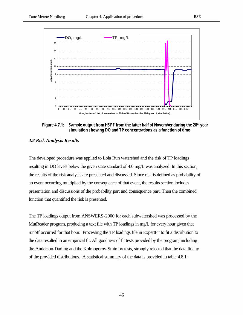
Tone Merete Nordberg Chapter 4. Application of procedure BSE
46
0
2
4
6
8
10
12
14
16
18
1 11 21 31 41 51 61 71 81 91 101 111 121 131 141 151 161 171 181 191 201 211 221 231
time, hr (from 21st of November to 30th of November the 28th year of simulation)
con
cen
trat
ion
, mg
/L
DO, mg/L TP, mg/L
Figure 4.7.1: Sample output from HSPF from the latter half of November during the 28th year
simulation showing DO and TP concentrations as a function of time
4.8 Risk Analysis Results
The developed procedure was applied to Lola Run watershed and the risk of TP loadings
resulting in DO levels below the given state standard of 4.0 mg/L was analyzed. In this section,
the results of the risk analysis are presented and discussed. Since risk is defined as probability of
an event occurring multiplied by the consequence of that event, the results section includes
presentation and discussions of the probability part and consequence part. Then the combined
function that quantified the risk is presented.
The TP loadings output from ANSWERS-2000 for each subwatershed was processed by the
MutReader program, producing a text file with TP loadings in mg/L for every hour given that
runoff occurred for that hour. Processing the TP loadings file in ExpertFit to fit a distribution to
the data resulted in an empirical fit. All goodness of fit tests provided by the program, including
the Anderson-Darling and the Kolmogorov-Smirnov tests, strongly rejected that the data fit any
of the provided distributions. A statistical summary of the data is provided in table 4.8.1.

Tone Merete Nordberg Chapter 4. Application of procedure BSE
47
Table 4.8.1. Statistical summary of TP loading output from ANSWERS-2000 based on 50 years of simulated weather data
Sample Characteristic Value Observation type Real valued Number of observations 4,069 Minimum observation 0.00000 Maximum observation 1.57248e6 mg/L Average 11,932.79460 mg/L Median 48.07890 mg/L Variance 5.05244e9 (mg/L)2 Coefficient of variation 5.95674 Skewness 13.20423 Kurtosis 216.66873 1st percentile 0.00000 mg/L 5th percentile 0.00000 mg/L 10th percentile 0.00000 mg/L 90th percentile 14,652.07154 mg/L 95th percentile 47,756.33642 mg/L 99th percentile 247,843.29501 mg/L
The high variance of data indicated the large dispersion of the data, which gives less meaning to
the mean value of the data set. The mean was 11932.8 mg/L compared to a median of 48.1 mg/L.
The data set also had a relatively high positive skewness indicating an asymmetric distribution.
The data range spanned from 0.0 to more than 1,500,000 mg/L, which is another indication of
the dispersion of the data.
ANSWERS-2000 produced extremely high TP loadings into the stream, including some TP
values that clearly exceeded a reasonable value. It was beyond the scope of this project to
investigate or correct this problem. As a result of this the TP loadings from ANSWERS-2000
were used only to demonstrate the developed procedure on Lola Run watershed and not in any
way to indicate the actual TP loadings in Lola Run. In the case of use for actual risk
quantification this problem would have to be rectified.
The endpoint for the risk quantification procedure to Lola Run was DO. The consequence was
measured in terms of the number of hours DO dropped below the standard divided by the total
number of hours the TP loadings exceeded the loading of interest. The result was the fraction of

Tone Merete Nordberg Chapter 4. Application of procedure BSE
48
time (or % if multiplied by 100) that the DO would drop below standard every time a TP loading
of interest occurred. This fraction increased as TP loadings increased, which was expected.
The results of the risk analysis (table 4.8.2) are presented in terms of cumulative probability
P[TP> xi]. The probability of occurrence decreased as the TP loadings increased, which was
expected. The number of hours DO was less than the standard, 4 mg/L, divided by the total
number of hours TP loadings were greater than xi increased as the TP loadings increased, which
was also expected. The risk was higher for the lower TP loadings than the higher TP loadings.
Smith et al. (1987) reported that an in-stream TP concentration greater 0.1 mg/L was
unacceptably high. The results show that the risk of a TP loading greater than 0.1 mg/L was
0.609 and the average number of hours the DO was less than the standard (4.0 mg/L) was 0.821
for every hour the TP loading exceeded the critical level, meaning that 82.1% of the time a TP
loading of 0.1 mg/L occurred the DO dropped below the standard. Smith et al. (1987) reported
in-stream concentrations of TP while the risk calculations were done based on a TP
concentration input into the stream. Lola Run was a small stream where dilution effects of TP
concentrations loaded into the stream can be assumed to be minimal. In watersheds draining a
bigger upland area with larger streams this assumption cannot be made, but considering baseflow
in the stream the dilution effect of the TP can be estimated. The results indicated that the many
small and intermediate size storms had a greater impact on in-stream water quality and
ecosystem health than the few large storms that have a very small probability of occurrence. This
indicates that the many smaller storms with small TP loadings but with a higher probability of
occurrence might be of more concern than the storm that produced the biggest TP loading as this
storm has a very small probability of occurring.

Tone Merete Nordberg Chapter 4. Application of procedure BSE
49
Table 4.8.2 Results of risk quantification for Lola Run watershed as a result of TP loadings into the system with a critical DO = 4.0 mg/L
Probability Consequence Risk
TP_critical P(x>TP_Critical) # hrs. DO < Std./ # hrs. TP > critical TP Risk_Level
mg/l 0.1 0.7417 0.8211 0.60890.5 0.7147 0.8298 0.59311.0 0.6967 0.8402 0.5853
5.00 0.6385 0.8580 0.547810.0 0.6030 0.8732 0.526520.0 0.5618 0.8933 0.501850.0 0.4974 0.9293 0.4623
100.0 0.4383 0.9568 0.4194500.0 0.3161 0.9938 0.3142
1000.0 0.2648 0.9991 0.26452000.0 0.2149 1.0000 0.2149
10000.0 0.1203 1.0000 0.1203
As a result of the earlier mentioned problem with high TP loadings into the stream, the risk as
quantified in table 4.8.2 is not intended to indicate actual risk resulting from TP loadings in Lola
Run. The data produced in this demonstration were used solely to demonstrate the developed
procedure. In developing the presented procedure only stochastic uncertainty, represented by
weather data, was accounted for. In addition to the stochastic uncertainty, the model and
parameter uncertainties will have a major effect on the outcome in a computer modeling based
procedure as presented here. To obtain more complete and accurate prediction of the
environmental risk as a result of TP loadings to surface waters, the model and parameter
uncertainty should be incorporated into the procedure. Considering all three types of uncertainty,
however, produces an extremely complex and difficult system to analyze.

Tone Merete Nordberg Chapter 6 Summary and Conclusions BSE
50
5.0 Potential Applications of the Risk Quantification Procedure
5.1 Introduction
The risk quantification procedure developed in this research was applied to Lola Run watershed
for a single management strategy for landuse and fertilizer application rates to demonstrate the
procedure and present a set of results that apply to Lola Run. The risk quantification procedure
developed has several more application areas than the one demonstrated. In this chapter the
different potential applications are discussed.
5.2 Applicable Uses of the Risk Quantification Procedure
The risk quantification procedure provides watershed management groups and stakeholders with
a method to calculate the risk the watershed is exposed to as a result of a particular pollutant
loading. For example, risk can be quantified using the described procedure for one or more
cropping/management scenarios. The resulting risk values can then be used to determine
alternative scenarios that meet an acceptable risk level (acceptable risk levels will vary
depending on the situation and will need to be determined by the concerned parties). For
example, as illustrated in Figure 5.2.1, risk associated with different fertilizer application
strategies can be compared. The fertilizer application strategies could be nitrogen (N) based
versus P-based. Each of the fertilizer strategies together with the crop of interest forms a
scenario. For example, scenario 1 could be N-based fertilizer application and corn silage while
scenario 2 could be P-based fertilizer application and wheat. For a specified risk level, one can
determine which, if any, of the evaluated fertilizer strategy/crop combinations would not exceed
the predetermined acceptable risk. The manager could then select from those scenario
combinations based on criteria such as economics, e.g., maximize net returns on the farm.

Tone Merete Nordberg Chapter 6 Summary and Conclusions BSE
51
Figure 5.2.1: Illustration of risk procedure to evaluate different management practices
Another application of the procedure is to evaluate the threat to in-stream ecosystems, benthic
community or fish. With some additional data/information, such as observed fish kill data with
corresponding relevant water quality parameters, the simulated water quality parameter values
could be correlated with number of fish kills. In the case of a stream with increased fish kills the
risk procedure can be used to identify and quantify risk of fish kills. If the length of time DO
must be below the standard to cause fish death was established, the procedure could be used to
estimate the number of dead fish per pollutant loading unit. This would provide watershed
managers with a tool to quantify the risk of fish kills as a result of pollutant loading.
Regulatory agencies can use the risk quantification procedure to identify acceptable risk levels
for watersheds, with respect to the current ecosystem health and water quality. Watersheds could
be categorized in terms of environmental sensitivity or current impairment, so that watersheds
with a low present impairment might be able to tolerate a higher risk level than watersheds with
high present impairment. The watershed stakeholders and managers could then use the risk level
set by regulatory agencies as an upper limit for pollutant loadings. How much, if any, reduction
in pollutant loading is needed to meet the risk level can be decided based on output from the NPS
model. The RiskCalc program written to calculate the risk in the procedure can also be used as a

Tone Merete Nordberg Chapter 6 Summary and Conclusions BSE
52
tool to identify the risk level resulting from different pollutant loadings. A screen shot of the
program is shown in figure 5.2.2.
Figure 5.2.2 Screen print of the RiskCalc program
Tone Merete Nordberg Chapter 6 Summary and Conclusions BSE
53
6.0 Summary and Conclusions The main objective of this research was to develop a procedure to quantify environmental risk of
pollutant loadings to surface waters including both the probability of an event occurring and the
consequence of that event. The objective was met with the development of the procedure
presented in this thesis. The procedure was developed conceptually with emphasis on linking the
probability of occurrence of an event with the resulting consequence quantified by NPS model
pollutant loading and an in-stream water quality model to simulate instream water chemistry and
transport. In implementing the procedure, ANSWERS-2000 was used for NPS modeling and
HSPF for in-stream modeling. In addition to the two main models, several VB programs were
written to facilitate and automate data processing and conversion from the output of one model
to the input of the next. The procedure was demonstrated on a small watershed in Rockingham
County, Virginia. The output of this demonstration showed that the many small phosphorus
loadings to surface water pose a greater risk to the watershed than the extreme storms, since
these storms might have a high consequence but a very small probability of occurring.
Pollutant loadings and consequences are often not directly linked in a way that is easy to model.
In order to obtain a better understanding of how the pollutant loadings and consequences are
related, more interdisciplinary research is needed. The effect of low DO levels and duration of
low DO levels on fish mortality combined with NPS modeling and stream flow modeling might
give a better understanding of ways to express the consequences of pollutant loadings in a
meaningful way with respect to biological endpoints. The complete picture of watershed risk is
very complex. In this research only the stochastic uncertainty was considered; both model
uncertainty and parameter uncertainty should be included for a more complete picture.
The risk quantification procedure could be improved in several ways. First making ANSWERS-
2000 a better model for urbanized areas would increase the areas in which the risk quantification
procedure could be applied. Increasing the hyetograph entries in ANSWERS-2000 to better
represent longer storms would decrease the possibility of misrepresentation of the storm and
more accurately estimate the NPS loading. A better understanding of the links between pollutant
loadings and biological endpoints would improve the risk output in terms of being a more direct

Tone Merete Nordberg Chapter 6 Summary and Conclusions BSE
54
link between pollutant loading and impact on biological endpoint. The risk quantification
procedure could also benefit from more research into possible ways to express the consequences.
Comparing results of the different ways to observed data should give a better understanding of
meaningful ways to express the consequence part of the procedure.
Third, using CLIGEN to generate the weather records requires a weather station from the list in
CLIGEN be selected. The closest available station might not have a weather pattern similar to
that of the watershed.
The above suggested improvements would improve the risk quantification procedure by
increasing the confidence in the results and find more useful ways to express the risk for
watershed managers and stakeholders. Weather data very much drives the outcome of the
procedure, hence the more accurate representation of the weather pattern in the watershed the
higher the confidence in the final result.

Tone Merete Nordberg References BSE
55
References
ASTM. 1985. Book of ASTM standards, 11.04. American Society for Testing Materials.
Philadelphia.
Andersen, H. V., J. Kjølholt, C. Poll, S. Ø. Dahl, F. Stuer-Lauridsen, F. Pedersen and
E. Bjørnstad. 1998. Environmental risk assessment of surface water and sediments in
Copenhagen Harbour. Water Science & Technology 37(6-7): 263-272.
Arnold, J. G., P. M. Allen and G. Bernhardt. 1993. A comprehensive surface-groundwater flow
model. Journal of Hydrology 142:47-69.
Bicknell, B. R., J. C. Imhoff, J. L. Kittle, A. S. Donigian and R. C. Johanson. 1993. Hydrological
simulation program-fortran (HSPF): User’s manual for release 10.0. EPA-600/3-84-066.
Environmental Research Laboratory, USEPA. Athens, Georgia.
ArcView. Redlands, California: Environmental Systems Research Institute.
Barnthouse, L. W., G. W. Suter II and S. M. Bartell. 1988. Quantifying risk of toxic chemicals to
aquatic populations and ecosystems. Chemosphere 17(8): 1487-1492.
Bouraoui, F. 1994. Development of a continuous, physically-based, distributed parameter,
nonpoint source model. PhD. dis., Biological Systems Engineering. Virginia Polytechnic
Institute and State University, Blacksburg.
Byne, W. 2000. Predicting sediment detachment and channel scouring in the process-based
planning model ANSWERS-2000. M.S. Thesis. Biological Systems Engineering, Virginia
Polytechnic Institute and State University, Blacksburg.
Chaves, H. M. L. and M. A. Nearing. 1991. Uncertainty analysis of the WEPP soil erosion
model. Transactions of the ASAE 34(6): 2437-2443.

Tone Merete Nordberg References BSE
56
Chow, V. T., D. R. Maidment, and L. W. Mays. 1988. Applied Hydrology. Surface Water, ch. 5,
166-170. New York: McGraw-Hill, Inc.
Correll, D. L. 1998. The role of phosphorus in the eutrophication of receiving waters: a review.
Journal of Environmental Quality 27: 261-266.
Correll, D. L. 1999. Phosphorus: A rate limiting nutrient in surface waters. Poultry Science 78:
674-682.
Eagleson, P. S. 1970. Dynamic Hydrology. New York: McGraw-Hill Book Company.
Evans, D. O., K. H. Nicholls, Y. C. Allen and M. J. McMurtry. 1996. Historical land use,
phosphorus loading, and loss of fish habitat in Lake Simcoe, Canada. Canadian Journal of
Fisheries and Aquatic Science 53(Supplement 1): 194-218.
Haan, C. T.1977. Statistical Methods in Hydrology. Ames, IA: The Iowa University Press.
Haan, C. T. 1989. Parametric uncertainty in hydrologic modeling. Transactions of the ASAE
32(1): 137-146.
Heatwole, C. D. November, 11 1999. Muddy Creek Farm Generation Procedure. Available:
http://www.isis.vt.edu/watershed/MC/FarmGenerationProcedure.doc. (01/30/01).
Henley, E. J. and H. Kumamoto. 1991. Probabilistic Risk Assessment. New York: The Institute
of Electrical and Electronics Engineering Press.
Hession, C. W., D. E. Storm, C. T. Haan, S. L. Burks and M. D. Matlock. 1996. A watershed-
level ecological risk assessment methodology. Water Resources Bulletin 32(5):1039-1054.

Tone Merete Nordberg References BSE
57
Hogg, R. V. and J. Ledolter. 1992. Applied Statistics for Engineers and Physical Scientists. New
York: Macmillan Publishing Company.
Hunsaker, C. T., R. L. Graham, G. W. Suter II, R. V. O’Neil, B. L. Jackson, and L. W.
Barnthouse. 1989. Regional ecological risk assessment: Theory and demonstration. Oak Ridge
National Laboratory. Oak Ridge, Tennessee.
James, L. G. 1988. Principles of farm irrigation system design. Irrigation requirements and
scheduling, ch. 1, 21-30. New York: John Wiley & Sons, Inc.
Kuczera, G. and E. Parent. 1998. Monte Carlo assessment of parameter uncertainty in conceptual
catchment models: the Metropolis algorithm. Journal of Hydrology 211: 69-85.
Law, A. M. and W. D. Kelton. 1991. Simulation Modeling and Analysis. McGraw-Hill. New
York.
Lenwood, W. H. Jr., M. C. Scott and W. D. Killen. 1998. Ecological risk assessment of copper
and cadmium in the surface waters of Chesapeake Bay watershed. Environmental Toxicology
and Chemistry 17(6): 1172-1189.
Matlock, M. D., D. E. Storm, J. G. Sabbagh, C. T. Haan, M. D. Smolen, and S. L. Burks. 1994.
An ecological risk assessment paradigm using the Spatially Integrated Model for Phosphorus
Loading and Erosion (SIMPLE). Journal of Aquatic Ecosystem Health 3: 287-294.
Microsoft Visual Basic. Redmond, Washington: Microsoft Corporation.
Moghissi, A. A. 1984. Risk assessment risk management – practice and prospects. Mechanical
Engineering 103(11):21-23.
Montgomery, R. H., D. V. Lee and K. H. Reckhow. 1983. Predicting variability in Lake Ontario
Phosphorus Model. Journal of Great Lakes 9(1):74-82.
Tone Merete Nordberg References BSE
58
Morgan, M. G. and M. Henrion. 1992. Uncertainty. Cambridge, England: Cambridge University
Press.
National Research Council. 1983. Risk Assessment in Federal Government: Managing the
Process. National Academy Press: Washington D. C.
Newbold, R. J. and J. W. Elwood. 1981. Measuring nutrient spiraling in streams. Canadian
Journal of Fisheries and Aquatic Science 38: 860-863.
Nicks, A. D., L. J. Lane and G. A. Gander. 1995. Technical Documentation USDA Water
Eosion Prediction Project (WEPP), Ch. 2 Weather Generator. West Lafayette, Indiana.
Novotny, V. and H. Olem. 1994. Water Quality Prevention Identification and Management for
Diffuse Pollution. New York: Van Nostrand Reinhold.
NRCS. June, 2000. SSURGO Documentation. Natural Resources Conservation Service
Available: http://gis.itc.nrcs.usda.gov/docs/SSURGO_Documentation.html. (January 2001).
Orvos, D. R. and J. Cairns Jr. 1991. Developing a risk assessment strategy for the Chesapeake
Bay. Hydrobiologia. 215:189-203.
Parson, S. C., J. M. Hamlett, P. D. Robillard and M. A. Foster. 1998. Determining the decision-
making risk from AGNPS simulations. Transactions of the ASAE 41(6): 1679-1688.
Paul, W. 1996. Monte Carlo and fuzzy approaches to environmental risk assessment in plant
production. Acta Horticulture no. 406: 425-432.
Power, M. and D. G. Dixon, G. Power. 1994. Perspectives on environmental risk assessment.
Journal of Aquatic Ecosystem Health 3: 69-79.
Tone Merete Nordberg References BSE
59
Reckhow, K. H. 1994.Water quality simulation modeling and uncertainty analysis for risk
assessment and decision making. Ecological Modeling 72:1-20.
Renard, K. G., G. R. Foster, G. A. Weesies, and J. P Porter. 1991. RUSLE revised universal soil
loss equation. Journal of Soil and Water Conservation Society 46: 30-33.
Rowe, W. D. 1977. An Anatomy of Risk. New York: John Wiley & Sons, Inc.
Rubinstein, R. Y. 1981. Simulation and the Monte Carlo Method. New York: John Wiley &
Sons, Inc.
Ruckelshaus, W. D. 1983. Science, risk, and public policy. Science 221:1026-1028.
Schindler, D. W. 1977. The evolution of phosphorus limitation in lakes. Science 195:260-262.
Schwab, G. O., D. D. Fangmeier, W. J. Elliot and R. K. Frevert. 1993. Soil and Water
Conservation Engineering. New York: John Wiley & Sons, Inc.
Sharpley, A. and H. Tunney. 2000. Phosphorus research strategies to meet agricultural and
environmental challenges of the 21st century. Journal of Environmental Quality 29:176-181.
Simpson, T. W., S. J. Donohue, G. W. Hawkins, M. M. Monnett, and J. C. Baker. 1992. The
development and implementation of the Virginia Agronomic Land Use Evaluation System
(VALUES). Report. Department of Crop and Soil Environmental Sciences, Virginia Polytechnic
Institute and State University, Blacksburg, Virginia.
Smith, R. A., R. B. Alexander and M. G. Wolman. 1987. Water-quality trends in the nation’s
rivers. Science 235:1607-1615.

Tone Merete Nordberg References BSE
60
Singh, V. P. 1995. Computer models of watershed hydrology. Hydrologic Simulation Program
Fortran (HSPF), ed. A. S. Donigian, Jr., ch. 12, 395-442. Highlands, Colorado: Water Resources
Publications.
State Water Control Board. 1997. Surface water standards with general, statewide application.
Richmond: Commonwealth of Virginia.
Stumm, W. 1992. Water, endangered ecosystem: assessment of chemical pollution. Journal of
Environmental Engineering 118(4):466-476.
Summers, K. J., H. T. Wilson and J. Kou. 1993. A method for quantifying the predicted
uncertainties associated with water quality models. Ecological Modeling 65:161-176.
Suter, G. W. II. 1993. Ecological Risk Assessment. Ann Arbor, MI: Lewis Publisher.
Suter, G. W. II. 1990. Endpoints for regional ecological risk assessments. Environmental
Management 14(1):9-23.
Suter, G. W. II., L. W. Barnthouse, and R. V. O’Neill. 1987. Treatment of risk in environmental
impact assessment. Environmental Management 11(3):295-303.
The Royal Observatory Greenwich. August 24, 2000. Leap Years. Available:
http://www.rog.nmm.ac.uk/leaflets/leapyear/leapyear.html. (December 20, 2000).
Ünlü, K., D. R. Nielsen and J. W. Biggar. 1990. Stochastic analysis of unsaturated flow: one-
dimensional Monte Carlo simulations and comparisons with spectral perturbation analysis and
field observations. Water Resources Research 26(9):2207-2218.
USGS. September 27, 2000. Surface Water and Water Quality Models Information
Clearinghouse. United States Geological Survey. Available:
http://smig.usgs.gov/SMIC/SMIC.html. (March, 2000).
Tone Merete Nordberg References BSE
61
Veith, T. L, T. M. Nordberg, M. L. Wolfe and T. A. Dillaha. QUESTIONS: A user friendly
interface to ANSWERS-2000. In preparation, Biological Systems Engineering. Virginia
Polytechnic Institute and State University, Blacksburg.
Vollenweider, R. A. and J. Kerekes. 1980. The loading concept as basis for controlling
eutrophication philosophy and preliminary results of the OECD programme on eutrophication.
Progress in Water Technology 12(2):5-38.
WDMUtil Release 1.2. Washington D.C.: EPA’s Office of Science and Technology (OST).
Whyte, A. V. and I. Burton (ed). 1980. Environmental Risk Assessment, SCOPE 15. New York:
John Wiley & Sons, Inc.
Wicks, J. M., J. C. Bathurst and C. W. Johnson. 1992. Calibrating SHE-soil erosion model for
different land covers. Journal of Irrigation and Drainage Engineering, ASCE 118(5):708-723.
Wilson, R. and E. A. C. Crouch. 1987. Risk assessment and comparisons: an introduction.
Science 236:267-270.

Tone Merete Nordberg Appendix A BSE
62
APPENDIX A: Percent Cloud Cover Calculations

Tone Merete Nordberg Appendix A BSE
63
Equations used to calculate cloud cover (Eagleson, 1970):
( )as R
Nn
R50.025.0 +=
( ) ( ) ( ) ( ) ( ) ( )
+= ssveda hSinCosCosSinSinhrhR δφδφπ
180/26714.1 0
( ) ( ) ( ) ( )2530 1061048.71085191.1126.12 φφ −− +−= ABShd
( )( ) ( )( ) ( )( ) ( )( )41138264 1061634.31068285.2102774.51011403.198387.0 JJJJrve−−−− +−+−
( )δφTanTanCoshs −= −1
−−
+++−=
θθθθθθ
πδ
3001480.03002697.0
2000907.02006758.0070257.0399912.0006918.0180SinCos
SinCosSinCos
)1(986.0 −= Jθ
Where: n/N = ratio between actual and possible hours of sunshine
Ra = extraterrestrial radiation (mm/day); hd0 = daytime hours at zero declination, hours; rve = radius vector of the earth; hs = sunrise to sunset hour angle in degrees;
Φ = location latitude in degrees (positive for north latitudes and negative for south latitudes)
δ = declination of the sun in degrees; θ = day of the year expressed in degrees; and
J = days from January 1st (e.g., J=1 for Jan. 1, J=2 for Jan. 2,…., J=365 for Dec. 31).
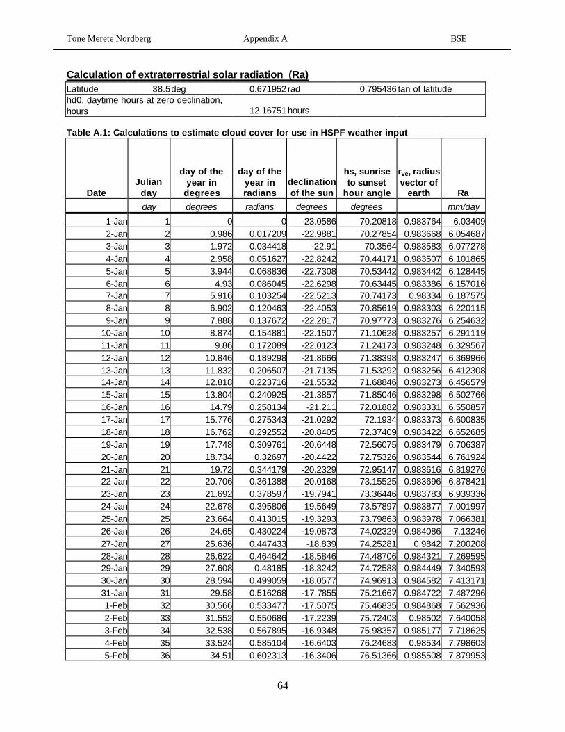
Tone Merete Nordberg Appendix A BSE
64
Calculation of extraterrestrial solar radiation (Ra) Latitude 38.5deg 0.671952 rad 0.795436 tan of latitude hd0, daytime hours at zero declination, hours 12.16751 hours Table A.1: Calculations to estimate cloud cover for use in HSPF weather input
Date Julian
day
day of the year in
degrees
day of the year in radians
declination of the sun
hs, sunrise to sunset
hour angle
rve, radius vector of
earth Ra
day degrees radians degrees degrees mm/day
1-Jan 1 0 0 -23.0586 70.20818 0.983764 6.034092-Jan 2 0.986 0.017209 -22.9881 70.27854 0.983668 6.0546873-Jan 3 1.972 0.034418 -22.91 70.3564 0.983583 6.0772784-Jan 4 2.958 0.051627 -22.8242 70.44171 0.983507 6.1018655-Jan 5 3.944 0.068836 -22.7308 70.53442 0.983442 6.1284456-Jan 6 4.93 0.086045 -22.6298 70.63445 0.983386 6.1570167-Jan 7 5.916 0.103254 -22.5213 70.74173 0.98334 6.1875758-Jan 8 6.902 0.120463 -22.4053 70.85619 0.983303 6.2201159-Jan 9 7.888 0.137672 -22.2817 70.97773 0.983276 6.254632
10-Jan 10 8.874 0.154881 -22.1507 71.10628 0.983257 6.29111911-Jan 11 9.86 0.172089 -22.0123 71.24173 0.983248 6.32956712-Jan 12 10.846 0.189298 -21.8666 71.38398 0.983247 6.36996613-Jan 13 11.832 0.206507 -21.7135 71.53292 0.983256 6.41230814-Jan 14 12.818 0.223716 -21.5532 71.68846 0.983273 6.45657915-Jan 15 13.804 0.240925 -21.3857 71.85046 0.983298 6.50276616-Jan 16 14.79 0.258134 -21.211 72.01882 0.983331 6.55085717-Jan 17 15.776 0.275343 -21.0292 72.1934 0.983373 6.60083518-Jan 18 16.762 0.292552 -20.8405 72.37409 0.983422 6.65268519-Jan 19 17.748 0.309761 -20.6448 72.56075 0.983479 6.70638720-Jan 20 18.734 0.32697 -20.4422 72.75326 0.983544 6.76192421-Jan 21 19.72 0.344179 -20.2329 72.95147 0.983616 6.81927622-Jan 22 20.706 0.361388 -20.0168 73.15525 0.983696 6.87842123-Jan 23 21.692 0.378597 -19.7941 73.36446 0.983783 6.93933624-Jan 24 22.678 0.395806 -19.5649 73.57897 0.983877 7.00199725-Jan 25 23.664 0.413015 -19.3293 73.79863 0.983978 7.06638126-Jan 26 24.65 0.430224 -19.0873 74.02329 0.984086 7.1324627-Jan 27 25.636 0.447433 -18.839 74.25281 0.9842 7.20020828-Jan 28 26.622 0.464642 -18.5846 74.48706 0.984321 7.26959529-Jan 29 27.608 0.48185 -18.3242 74.72588 0.984449 7.34059330-Jan 30 28.594 0.499059 -18.0577 74.96913 0.984582 7.41317131-Jan 31 29.58 0.516268 -17.7855 75.21667 0.984722 7.4872961-Feb 32 30.566 0.533477 -17.5075 75.46835 0.984868 7.5629362-Feb 33 31.552 0.550686 -17.2239 75.72403 0.98502 7.6400583-Feb 34 32.538 0.567895 -16.9348 75.98357 0.985177 7.7186254-Feb 35 33.524 0.585104 -16.6403 76.24683 0.98534 7.7986035-Feb 36 34.51 0.602313 -16.3406 76.51366 0.985508 7.879953

Tone Merete Nordberg Appendix A BSE
65
Date Julian
day
day of the year in
degrees
day of the year in radians
declination of the sun
hs, sunrise to sunset
hour angle
rve, radius vector of
earth Ra day degrees radians degrees degrees mm/day
6-Feb 37 35.496 0.619522 -16.0357 76.78393 0.985682 7.9626397-Feb 38 36.482 0.636731 -15.7258 77.05751 0.985861 8.0466228-Feb 39 37.468 0.65394 -15.4109 77.33425 0.986044 8.1318639-Feb 40 38.454 0.671149 -15.0914 77.61402 0.986233 8.21832
10-Feb 41 39.44 0.688358 -14.7671 77.8967 0.986427 8.30595311-Feb 42 40.426 0.705567 -14.4384 78.18215 0.986625 8.3947212-Feb 43 41.412 0.722776 -14.1052 78.47024 0.986828 8.48457813-Feb 44 42.398 0.739985 -13.7678 78.76086 0.987035 8.57548514-Feb 45 43.384 0.757194 -13.4263 79.05387 0.987247 8.66739815-Feb 46 44.37 0.774403 -13.0808 79.34916 0.987463 8.76027116-Feb 47 45.356 0.791612 -12.7315 79.64661 0.987683 8.8540617-Feb 48 46.342 0.80882 -12.3785 79.94611 0.987907 8.94872118-Feb 49 47.328 0.826029 -12.0218 80.24754 0.988134 9.04420819-Feb 50 48.314 0.843238 -11.6618 80.55079 0.988366 9.14047520-Feb 51 49.3 0.860447 -11.2984 80.85575 0.988601 9.23747621-Feb 52 50.286 0.877656 -10.9319 81.16233 0.988839 9.33516622-Feb 53 51.272 0.894865 -10.5623 81.47041 0.989081 9.43349823-Feb 54 52.258 0.912074 -10.1899 81.77989 0.989326 9.53242624-Feb 55 53.244 0.929283 -9.81468 82.09069 0.989574 9.63190425-Feb 56 54.23 0.946492 -9.43688 82.4027 0.989825 9.73188526-Feb 57 55.216 0.963701 -9.05661 82.71583 0.99008 9.83232327-Feb 58 56.202 0.98091 -8.67402 83.03 0.990336 9.93317228-Feb 59 57.188 0.998119 -8.28923 83.34511 0.990596 10.034391-Mar 60 58.174 1.015328 -7.90238 83.66108 0.990858 10.135922-Mar 61 59.16 1.032537 -7.51361 83.97782 0.991123 10.237733-Mar 62 60.146 1.049746 -7.12307 84.29526 0.99139 10.339774-Mar 63 61.132 1.066955 -6.73088 84.61332 0.991659 10.441995-Mar 64 62.118 1.084164 -6.33717 84.93192 0.99193 10.544356-Mar 65 63.104 1.101373 -5.94209 85.25099 0.992204 10.646817-Mar 66 64.09 1.118582 -5.54577 85.57046 0.992479 10.749328-Mar 67 65.076 1.13579 -5.14834 85.89025 0.992756 10.851859-Mar 68 66.062 1.152999 -4.74993 86.2103 0.993035 10.95434
10-Mar 69 67.048 1.170208 -4.35066 86.53054 0.993315 11.0567611-Mar 70 68.034 1.187417 -3.95068 86.85091 0.993597 11.1590712-Mar 71 69.02 1.204626 -3.55011 87.17134 0.993881 11.2612213-Mar 72 70.006 1.221835 -3.14908 87.49179 0.994165 11.3631814-Mar 73 70.992 1.239044 -2.7477 87.81217 0.994451 11.4649115-Mar 74 71.978 1.256253 -2.34611 88.13245 0.994738 11.5663716-Mar 75 72.964 1.273462 -1.94443 88.45255 0.995026 11.6675217-Mar 76 73.95 1.290671 -1.54277 88.77243 0.995315 11.7683418-Mar 77 74.936 1.30788 -1.14126 89.09204 0.995605 11.8687719-Mar 78 75.922 1.325089 -0.74002 89.41132 0.995895 11.9687920-Mar 79 76.908 1.342298 -0.33917 89.73021 0.996186 12.0683721-Mar 80 77.894 1.359507 0.061191 90.04867 0.996478 12.16747
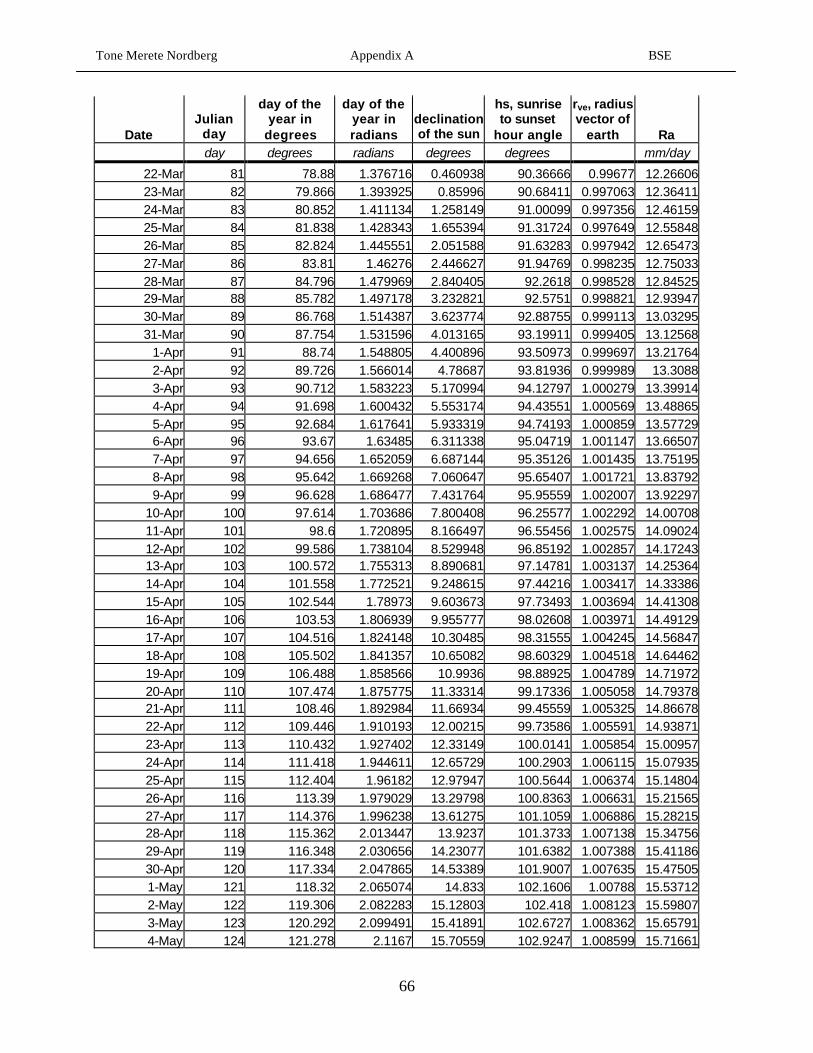
Tone Merete Nordberg Appendix A BSE
66
Date Julian
day
day of the year in
degrees
day of the year in radians
declination of the sun
hs, sunrise to sunset
hour angle
rve, radius vector of
earth Ra day degrees radians degrees degrees mm/day
22-Mar 81 78.88 1.376716 0.460938 90.36666 0.99677 12.2660623-Mar 82 79.866 1.393925 0.85996 90.68411 0.997063 12.3641124-Mar 83 80.852 1.411134 1.258149 91.00099 0.997356 12.4615925-Mar 84 81.838 1.428343 1.655394 91.31724 0.997649 12.5584826-Mar 85 82.824 1.445551 2.051588 91.63283 0.997942 12.6547327-Mar 86 83.81 1.46276 2.446627 91.94769 0.998235 12.7503328-Mar 87 84.796 1.479969 2.840405 92.2618 0.998528 12.8452529-Mar 88 85.782 1.497178 3.232821 92.5751 0.998821 12.9394730-Mar 89 86.768 1.514387 3.623774 92.88755 0.999113 13.0329531-Mar 90 87.754 1.531596 4.013165 93.19911 0.999405 13.12568
1-Apr 91 88.74 1.548805 4.400896 93.50973 0.999697 13.217642-Apr 92 89.726 1.566014 4.78687 93.81936 0.999989 13.30883-Apr 93 90.712 1.583223 5.170994 94.12797 1.000279 13.399144-Apr 94 91.698 1.600432 5.553174 94.43551 1.000569 13.488655-Apr 95 92.684 1.617641 5.933319 94.74193 1.000859 13.577296-Apr 96 93.67 1.63485 6.311338 95.04719 1.001147 13.665077-Apr 97 94.656 1.652059 6.687144 95.35126 1.001435 13.751958-Apr 98 95.642 1.669268 7.060647 95.65407 1.001721 13.837929-Apr 99 96.628 1.686477 7.431764 95.95559 1.002007 13.92297
10-Apr 100 97.614 1.703686 7.800408 96.25577 1.002292 14.0070811-Apr 101 98.6 1.720895 8.166497 96.55456 1.002575 14.0902412-Apr 102 99.586 1.738104 8.529948 96.85192 1.002857 14.1724313-Apr 103 100.572 1.755313 8.890681 97.14781 1.003137 14.2536414-Apr 104 101.558 1.772521 9.248615 97.44216 1.003417 14.3338615-Apr 105 102.544 1.78973 9.603673 97.73493 1.003694 14.4130816-Apr 106 103.53 1.806939 9.955777 98.02608 1.003971 14.4912917-Apr 107 104.516 1.824148 10.30485 98.31555 1.004245 14.5684718-Apr 108 105.502 1.841357 10.65082 98.60329 1.004518 14.6446219-Apr 109 106.488 1.858566 10.9936 98.88925 1.004789 14.7197220-Apr 110 107.474 1.875775 11.33314 99.17336 1.005058 14.7937821-Apr 111 108.46 1.892984 11.66934 99.45559 1.005325 14.8667822-Apr 112 109.446 1.910193 12.00215 99.73586 1.005591 14.9387123-Apr 113 110.432 1.927402 12.33149 100.0141 1.005854 15.0095724-Apr 114 111.418 1.944611 12.65729 100.2903 1.006115 15.0793525-Apr 115 112.404 1.96182 12.97947 100.5644 1.006374 15.1480426-Apr 116 113.39 1.979029 13.29798 100.8363 1.006631 15.2156527-Apr 117 114.376 1.996238 13.61275 101.1059 1.006886 15.2821528-Apr 118 115.362 2.013447 13.9237 101.3733 1.007138 15.3475629-Apr 119 116.348 2.030656 14.23077 101.6382 1.007388 15.4118630-Apr 120 117.334 2.047865 14.53389 101.9007 1.007635 15.475051-May 121 118.32 2.065074 14.833 102.1606 1.00788 15.537122-May 122 119.306 2.082283 15.12803 102.418 1.008123 15.598073-May 123 120.292 2.099491 15.41891 102.6727 1.008362 15.657914-May 124 121.278 2.1167 15.70559 102.9247 1.008599 15.71661
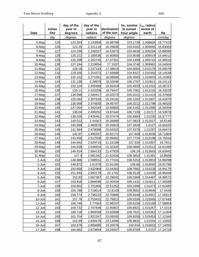
Tone Merete Nordberg Appendix A BSE
67
Date Julian
day
day of the year in
degrees
day of the year in radians
declination of the sun
hs, sunrise to sunset
hour angle
rve, radius vector of
earth Ra day degrees radians degrees degrees mm/day
5-May 125 122.264 2.133909 15.98799 103.1739 1.008834 15.774196-May 126 123.25 2.151118 16.26606 103.4202 1.009065 15.830637-May 127 124.236 2.168327 16.53973 103.6635 1.009294 15.885958-May 128 125.222 2.185536 16.80893 103.9038 1.009519 15.940129-May 129 126.208 2.202745 17.07361 104.1409 1.009742 15.99315
10-May 130 127.194 2.219954 17.3337 104.3748 1.009962 16.0450411-May 131 128.18 2.237163 17.58915 104.6054 1.010179 16.0957912-May 132 129.166 2.254372 17.83988 104.8327 1.010393 16.1453813-May 133 130.152 2.271581 18.08584 105.0565 1.010603 16.1938314-May 134 131.138 2.28879 18.32696 105.2767 1.010811 16.2411315-May 135 132.124 2.305999 18.56319 105.4933 1.011015 16.2872716-May 136 133.11 2.323208 18.79447 105.7061 1.011216 16.3322517-May 137 134.096 2.340417 19.02073 105.9151 1.011413 16.3760818-May 138 135.082 2.357626 19.24191 106.1202 1.011607 16.4187519-May 139 136.068 2.374835 19.45797 106.3212 1.011798 16.4602520-May 140 137.054 2.392044 19.66883 106.5182 1.011986 16.5005921-May 141 138.04 2.409252 19.87444 106.7109 1.01217 16.5397622-May 142 139.026 2.426461 20.07474 106.8993 1.01235 16.5777723-May 143 140.012 2.44367 20.26968 107.0833 1.012527 16.614624-May 144 140.998 2.460879 20.45919 107.2628 1.0127 16.6502525-May 145 141.984 2.478088 20.64322 107.4378 1.01287 16.6847426-May 146 142.97 2.495297 20.82172 107.608 1.013036 16.7180427-May 147 143.956 2.512506 20.99462 107.7734 1.013198 16.7501628-May 148 144.942 2.529715 21.16189 107.934 1.013357 16.781129-May 149 145.928 2.546924 21.32345 108.0895 1.013512 16.8108630-May 150 146.914 2.564133 21.47926 108.24 1.013663 16.8394231-May 151 147.9 2.581342 21.62926 108.3853 1.01381 16.8668
1-Jun 152 148.886 2.598551 21.77341 108.5253 1.013953 16.892982-Jun 153 149.872 2.61576 21.91165 108.66 1.014093 16.917963-Jun 154 150.858 2.632969 22.04393 108.7892 1.014228 16.941754-Jun 155 151.844 2.650178 22.1702 108.9128 1.01436 16.964345-Jun 156 152.83 2.667387 22.29042 109.0308 1.014487 16.985726-Jun 157 153.816 2.684596 22.40454 109.1431 1.014611 17.005897-Jun 158 154.802 2.701805 22.51252 109.2496 1.01473 17.024858-Jun 159 155.788 2.719014 22.6143 109.3502 1.014846 17.04269-Jun 160 156.774 2.736222 22.70985 109.4448 1.014957 17.05913
10-Jun 161 157.76 2.753431 22.79912 109.5334 1.015065 17.0744511-Jun 162 158.746 2.77064 22.88207 109.6158 1.015168 17.0885412-Jun 163 159.732 2.787849 22.95867 109.6921 1.015267 17.101413-Jun 164 160.718 2.805058 23.02888 109.7621 1.015362 17.1130414-Jun 165 161.704 2.822267 23.09265 109.8258 1.015453 17.1234415-Jun 166 162.69 2.839476 23.14996 109.8831 1.01554 17.1326216-Jun 167 163.676 2.856685 23.20078 109.934 1.015622 17.1405517-Jun 168 164.662 2.873894 23.24507 109.9784 1.0157 17.14724

Tone Merete Nordberg Appendix A BSE
68
Date Julian
day
day of the year in
degrees
day of the year in radians
declination of the sun
hs, sunrise to sunset
hour angle
rve, radius vector of
earth Ra day degrees radians degrees degrees mm/day
18-Jun 169 165.648 2.891103 23.2828 110.0162 1.015774 17.1526919-Jun 170 166.634 2.908312 23.31395 110.0475 1.015844 17.1568920-Jun 171 167.62 2.925521 23.33848 110.0721 1.015909 17.1598521-Jun 172 168.606 2.94273 23.35639 110.0901 1.015971 17.1615522-Jun 173 169.592 2.959939 23.36764 110.1014 1.016027 17.1619923-Jun 174 170.578 2.977148 23.37222 110.106 1.01608 17.1611824-Jun 175 171.564 2.994357 23.3701 110.1039 1.016128 17.159125-Jun 176 172.55 3.011566 23.36128 110.095 1.016172 17.1557726-Jun 177 173.536 3.028775 23.34574 110.0794 1.016212 17.1511727-Jun 178 174.522 3.045984 23.32348 110.057 1.016247 17.1452928-Jun 179 175.508 3.063192 23.29447 110.0279 1.016278 17.1381529-Jun 180 176.494 3.080401 23.25872 109.992 1.016304 17.1297430-Jun 181 177.48 3.09761 23.21623 109.9495 1.016326 17.12005
1-Jul 182 178.466 3.114819 23.16699 109.9001 1.016344 17.109092-Jul 183 179.452 3.132028 23.111 109.8441 1.016358 17.096843-Jul 184 180.438 3.149237 23.04827 109.7815 1.016367 17.083324-Jul 185 181.424 3.166446 22.9788 109.7122 1.016371 17.068515-Jul 186 182.41 3.183655 22.90261 109.6363 1.016372 17.052426-Jul 187 183.396 3.200864 22.8197 109.5538 1.016368 17.035057-Jul 188 184.382 3.218073 22.73009 109.4649 1.016359 17.016398-Jul 189 185.368 3.235282 22.6338 109.3695 1.016347 16.996449-Jul 190 186.354 3.252491 22.53085 109.2677 1.016329 16.97521
10-Jul 191 187.34 3.2697 22.42125 109.1596 1.016308 16.9526911-Jul 192 188.326 3.286909 22.30504 109.0452 1.016282 16.9288812-Jul 193 189.312 3.304118 22.18224 108.9246 1.016252 16.9037813-Jul 194 190.298 3.321327 22.05289 108.7979 1.016217 16.877414-Jul 195 191.284 3.338536 21.91701 108.6652 1.016178 16.8497315-Jul 196 192.27 3.355745 21.77463 108.5265 1.016135 16.8207716-Jul 197 193.256 3.372953 21.62581 108.3819 1.016087 16.7905317-Jul 198 194.242 3.390162 21.47058 108.2316 1.016036 16.75918-Jul 199 195.228 3.407371 21.30899 108.0756 1.015979 16.7261919-Jul 200 196.214 3.42458 21.14107 107.914 1.015919 16.6920920-Jul 201 197.2 3.441789 20.96688 107.7468 1.015854 16.6567221-Jul 202 198.186 3.458998 20.78648 107.5743 1.015785 16.6200622-Jul 203 199.172 3.476207 20.59991 107.3965 1.015712 16.5821423-Jul 204 200.158 3.493416 20.40723 107.2136 1.015634 16.5429324-Jul 205 201.144 3.510625 20.2085 107.0255 1.015552 16.5024625-Jul 206 202.13 3.527834 20.00379 106.8325 1.015466 16.4607326-Jul 207 203.116 3.545043 19.79315 106.6346 1.015376 16.4177327-Jul 208 204.102 3.562252 19.57666 106.432 1.015282 16.3734728-Jul 209 205.088 3.579461 19.35438 106.2247 1.015184 16.3279629-Jul 210 206.074 3.59667 19.12638 106.0129 1.015081 16.2811930-Jul 211 207.06 3.613879 18.89274 105.7968 1.014974 16.2331931-Jul 212 208.046 3.631088 18.65353 105.5763 1.014863 16.18394

Tone Merete Nordberg Appendix A BSE
69
Date Julian
day
day of the year in
degrees
day of the year in radians
declination of the sun
hs, sunrise to sunset
hour angle
rve, radius vector of
earth Ra day degrees radians degrees degrees mm/day
1-Aug 213 209.032 3.648297 18.40883 105.3516 1.014749 16.133462-Aug 214 210.018 3.665506 18.15872 105.1229 1.01463 16.081763-Aug 215 211.004 3.682715 17.90328 104.8903 1.014507 16.028834-Aug 216 211.99 3.699923 17.64259 104.6538 1.01438 15.974695-Aug 217 212.976 3.717132 17.37675 104.4136 1.014249 15.919346-Aug 218 213.962 3.734341 17.10583 104.1698 1.014114 15.86287-Aug 219 214.948 3.75155 16.82993 103.9225 1.013975 15.805078-Aug 220 215.934 3.768759 16.54914 103.6719 1.013833 15.746159-Aug 221 216.92 3.785968 16.26355 103.4179 1.013686 15.68606
10-Aug 222 217.906 3.803177 15.97326 103.1609 1.013536 15.6248111-Aug 223 218.892 3.820386 15.67835 102.9007 1.013382 15.5624112-Aug 224 219.878 3.837595 15.37893 102.6377 1.013224 15.4988713-Aug 225 220.864 3.854804 15.0751 102.3718 1.013062 15.4341914-Aug 226 221.85 3.872013 14.76695 102.1032 1.012897 15.368415-Aug 227 222.836 3.889222 14.45458 101.8319 1.012728 15.301516-Aug 228 223.822 3.906431 14.1381 101.5581 1.012555 15.233517-Aug 229 224.808 3.92364 13.81762 101.2819 1.012379 15.1644218-Aug 230 225.794 3.940849 13.49323 101.0034 1.012199 15.0942719-Aug 231 226.78 3.958058 13.16503 100.7227 1.012016 15.0230720-Aug 232 227.766 3.975267 12.83315 100.4398 1.011829 14.9508321-Aug 233 228.752 3.992476 12.49767 100.1549 1.011639 14.8775622-Aug 234 229.738 4.009685 12.15871 99.86803 1.011446 14.8032823-Aug 235 230.724 4.026893 11.81638 99.5793 1.011249 14.72824-Aug 236 231.71 4.044102 11.47078 99.2888 1.011049 14.6517525-Aug 237 232.696 4.061311 11.12203 98.9966 1.010845 14.5745426-Aug 238 233.682 4.07852 10.77022 98.7028 1.010639 14.4963827-Aug 239 234.668 4.095729 10.41548 98.40747 1.010429 14.4172928-Aug 240 235.654 4.112938 10.05792 98.11069 1.010216 14.337329-Aug 241 236.64 4.130147 9.69763 97.81254 1.01 14.2564230-Aug 242 237.626 4.147356 9.334737 97.5131 1.009781 14.1746731-Aug 243 238.612 4.164565 8.969346 97.21243 1.009559 14.092061-Sep 244 239.598 4.181774 8.601569 96.91061 1.009334 14.008632-Sep 245 240.584 4.198983 8.231515 96.6077 1.009106 13.924393-Sep 246 241.57 4.216192 7.859296 96.30378 1.008875 13.839364-Sep 247 242.556 4.233401 7.485021 95.99891 1.008641 13.753565-Sep 248 243.542 4.25061 7.1088 95.69315 1.008405 13.667016-Sep 249 244.528 4.267819 6.730745 95.38657 1.008166 13.579757-Sep 250 245.514 4.285028 6.350964 95.07923 1.007925 13.491788-Sep 251 246.5 4.302237 5.969567 94.77118 1.007681 13.403149-Sep 252 247.486 4.319446 5.586663 94.46248 1.007434 13.31384
10-Sep 253 248.472 4.336654 5.202361 94.15319 1.007185 13.2239211-Sep 254 249.458 4.353863 4.81677 93.84337 1.006933 13.1333912-Sep 255 250.444 4.371072 4.429998 93.53306 1.00668 13.0422813-Sep 256 251.43 4.388281 4.042153 93.22232 1.006424 12.95062
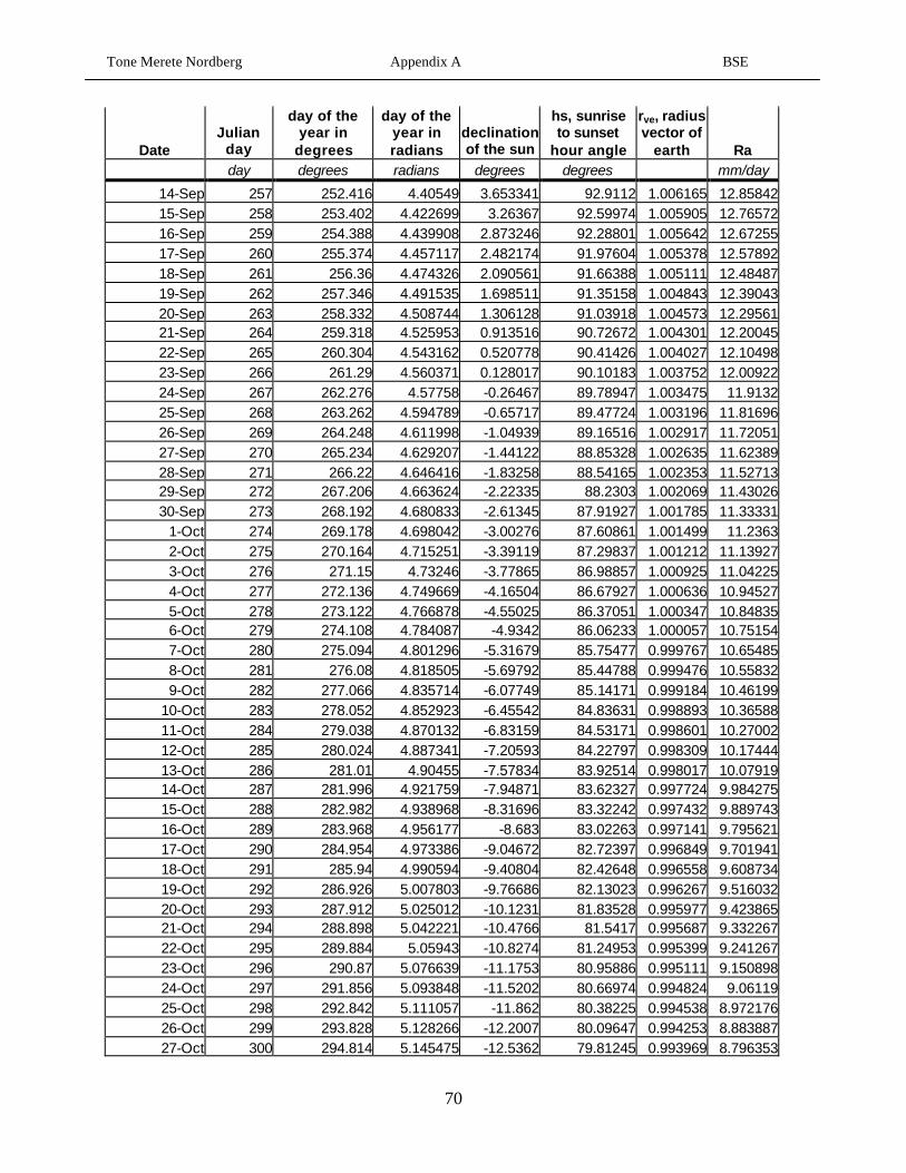
Tone Merete Nordberg Appendix A BSE
70
Date Julian
day
day of the year in
degrees
day of the year in radians
declination of the sun
hs, sunrise to sunset
hour angle
rve, radius vector of
earth Ra day degrees radians degrees degrees mm/day
14-Sep 257 252.416 4.40549 3.653341 92.9112 1.006165 12.8584215-Sep 258 253.402 4.422699 3.26367 92.59974 1.005905 12.7657216-Sep 259 254.388 4.439908 2.873246 92.28801 1.005642 12.6725517-Sep 260 255.374 4.457117 2.482174 91.97604 1.005378 12.5789218-Sep 261 256.36 4.474326 2.090561 91.66388 1.005111 12.4848719-Sep 262 257.346 4.491535 1.698511 91.35158 1.004843 12.3904320-Sep 263 258.332 4.508744 1.306128 91.03918 1.004573 12.2956121-Sep 264 259.318 4.525953 0.913516 90.72672 1.004301 12.2004522-Sep 265 260.304 4.543162 0.520778 90.41426 1.004027 12.1049823-Sep 266 261.29 4.560371 0.128017 90.10183 1.003752 12.0092224-Sep 267 262.276 4.57758 -0.26467 89.78947 1.003475 11.913225-Sep 268 263.262 4.594789 -0.65717 89.47724 1.003196 11.8169626-Sep 269 264.248 4.611998 -1.04939 89.16516 1.002917 11.7205127-Sep 270 265.234 4.629207 -1.44122 88.85328 1.002635 11.6238928-Sep 271 266.22 4.646416 -1.83258 88.54165 1.002353 11.5271329-Sep 272 267.206 4.663624 -2.22335 88.2303 1.002069 11.4302630-Sep 273 268.192 4.680833 -2.61345 87.91927 1.001785 11.33331
1-Oct 274 269.178 4.698042 -3.00276 87.60861 1.001499 11.23632-Oct 275 270.164 4.715251 -3.39119 87.29837 1.001212 11.139273-Oct 276 271.15 4.73246 -3.77865 86.98857 1.000925 11.042254-Oct 277 272.136 4.749669 -4.16504 86.67927 1.000636 10.945275-Oct 278 273.122 4.766878 -4.55025 86.37051 1.000347 10.848356-Oct 279 274.108 4.784087 -4.9342 86.06233 1.000057 10.751547-Oct 280 275.094 4.801296 -5.31679 85.75477 0.999767 10.654858-Oct 281 276.08 4.818505 -5.69792 85.44788 0.999476 10.558329-Oct 282 277.066 4.835714 -6.07749 85.14171 0.999184 10.46199
10-Oct 283 278.052 4.852923 -6.45542 84.83631 0.998893 10.3658811-Oct 284 279.038 4.870132 -6.83159 84.53171 0.998601 10.2700212-Oct 285 280.024 4.887341 -7.20593 84.22797 0.998309 10.1744413-Oct 286 281.01 4.90455 -7.57834 83.92514 0.998017 10.0791914-Oct 287 281.996 4.921759 -7.94871 83.62327 0.997724 9.98427515-Oct 288 282.982 4.938968 -8.31696 83.32242 0.997432 9.88974316-Oct 289 283.968 4.956177 -8.683 83.02263 0.997141 9.79562117-Oct 290 284.954 4.973386 -9.04672 82.72397 0.996849 9.70194118-Oct 291 285.94 4.990594 -9.40804 82.42648 0.996558 9.60873419-Oct 292 286.926 5.007803 -9.76686 82.13023 0.996267 9.51603220-Oct 293 287.912 5.025012 -10.1231 81.83528 0.995977 9.42386521-Oct 294 288.898 5.042221 -10.4766 81.5417 0.995687 9.33226722-Oct 295 289.884 5.05943 -10.8274 81.24953 0.995399 9.24126723-Oct 296 290.87 5.076639 -11.1753 80.95886 0.995111 9.15089824-Oct 297 291.856 5.093848 -11.5202 80.66974 0.994824 9.0611925-Oct 298 292.842 5.111057 -11.862 80.38225 0.994538 8.97217626-Oct 299 293.828 5.128266 -12.2007 80.09647 0.994253 8.88388727-Oct 300 294.814 5.145475 -12.5362 79.81245 0.993969 8.796353

Tone Merete Nordberg Appendix A BSE
71
Date Julian
day
day of the year in
degrees
day of the year in radians
declination of the sun
hs, sunrise to sunset
hour angle
rve, radius vector of
earth Ra day degrees radians degrees degrees mm/day
28-Oct 301 295.8 5.162684 -12.8683 79.53029 0.993687 8.70960629-Oct 302 296.786 5.179893 -13.1969 79.25006 0.993406 8.62367830-Oct 303 297.772 5.197102 -13.5221 78.97184 0.993126 8.53859831-Oct 304 298.758 5.214311 -13.8436 78.69571 0.992849 8.4543981-Nov 305 299.744 5.23152 -14.1614 78.42177 0.992573 8.3711092-Nov 306 300.73 5.248729 -14.4754 78.15009 0.992298 8.288763-Nov 307 301.716 5.265938 -14.7854 77.88077 0.992026 8.2073834-Nov 308 302.702 5.283147 -15.0915 77.6139 0.991756 8.1270085-Nov 309 303.688 5.300355 -15.3935 77.34958 0.991488 8.0476656-Nov 310 304.674 5.317564 -15.6913 77.0879 0.991222 7.9693837-Nov 311 305.66 5.334773 -15.9848 76.82897 0.990958 7.8921928-Nov 312 306.646 5.351982 -16.2739 76.57289 0.990697 7.8161229-Nov 313 307.632 5.369191 -16.5585 76.31975 0.990439 7.741202
10-Nov 314 308.618 5.3864 -16.8386 76.06968 0.990183 7.6674611-Nov 315 309.604 5.403609 -17.1141 75.82278 0.98993 7.59492612-Nov 316 310.59 5.420818 -17.3848 75.57915 0.98968 7.52362713-Nov 317 311.576 5.438027 -17.6506 75.33892 0.989433 7.45359314-Nov 318 312.562 5.455236 -17.9115 75.1022 0.989189 7.38484915-Nov 319 313.548 5.472445 -18.1674 74.86911 0.988949 7.31742516-Nov 320 314.534 5.489654 -18.4182 74.63977 0.988711 7.25134717-Nov 321 315.52 5.506863 -18.6638 74.4143 0.988477 7.18664118-Nov 322 316.506 5.524072 -18.904 74.19281 0.988247 7.12333419-Nov 323 317.492 5.541281 -19.1389 73.97545 0.988021 7.06145220-Nov 324 318.478 5.55849 -19.3683 73.76233 0.987798 7.00102121-Nov 325 319.464 5.575699 -19.5921 73.55358 0.987579 6.94206522-Nov 326 320.45 5.592908 -19.8103 73.34932 0.987365 6.8846123-Nov 327 321.436 5.610117 -20.0227 73.1497 0.987154 6.82867924-Nov 328 322.422 5.627325 -20.2293 72.95483 0.986948 6.77429725-Nov 329 323.408 5.644534 -20.43 72.76484 0.986747 6.72148626-Nov 330 324.394 5.661743 -20.6247 72.57987 0.986549 6.6702727-Nov 331 325.38 5.678952 -20.8133 72.40005 0.986357 6.62067128-Nov 332 326.366 5.696161 -20.9957 72.22551 0.986169 6.5727129-Nov 333 327.352 5.71337 -21.1719 72.05637 0.985987 6.5264130-Nov 334 328.338 5.730579 -21.3418 71.89277 0.985809 6.481791-Dec 335 329.324 5.747788 -21.5053 71.73482 0.985637 6.4388722-Dec 336 330.31 5.764997 -21.6623 71.58267 0.98547 6.3976753-Dec 337 331.296 5.782206 -21.8127 71.43643 0.985308 6.3582184-Dec 338 332.282 5.799415 -21.9565 71.29622 0.985152 6.3205195-Dec 339 333.268 5.816624 -22.0937 71.16217 0.985002 6.2845976-Dec 340 334.254 5.833833 -22.224 71.0344 0.984858 6.2504687-Dec 341 335.24 5.851042 -22.3475 70.91301 0.984719 6.2181518-Dec 342 336.226 5.868251 -22.4642 70.79812 0.984587 6.187669-Dec 343 337.212 5.88546 -22.5738 70.68984 0.984461 6.159012
10-Dec 344 338.198 5.902669 -22.6765 70.58828 0.984341 6.132221

Tone Merete Nordberg Appendix A BSE
72
Date Julian
day
day of the year in
degrees
day of the year in radians
declination of the sun
hs, sunrise to sunset
hour angle
rve, radius vector of
earth Ra day degrees radians degrees degrees mm/day
11-Dec 345 339.184 5.919878 -22.772 70.49354 0.984228 6.10730112-Dec 346 340.17 5.937087 -22.8604 70.4057 0.984122 6.08426713-Dec 347 341.156 5.954295 -22.9416 70.32487 0.984022 6.06313114-Dec 348 342.142 5.971504 -23.0156 70.25113 0.983929 6.04390415-Dec 349 343.128 5.988713 -23.0823 70.18457 0.983844 6.026616-Dec 350 344.114 6.005922 -23.1416 70.12525 0.983766 6.01122817-Dec 351 345.1 6.023131 -23.1936 70.07326 0.983695 5.99779818-Dec 352 346.086 6.04034 -23.2381 70.02865 0.983631 5.9863219-Dec 353 347.072 6.057549 -23.2751 69.99149 0.983575 5.97680320-Dec 354 348.058 6.074758 -23.3047 69.96183 0.983527 5.96925421-Dec 355 349.044 6.091967 -23.3267 69.93972 0.983487 5.96367922-Dec 356 350.03 6.109176 -23.3412 69.92519 0.983455 5.96008723-Dec 357 351.016 6.126385 -23.3481 69.91828 0.983432 5.95848124-Dec 358 352.002 6.143594 -23.3473 69.91901 0.983416 5.95886625-Dec 359 352.988 6.160803 -23.339 69.9274 0.98341 5.96124726-Dec 360 353.974 6.178012 -23.323 69.94347 0.983412 5.96562527-Dec 361 354.96 6.195221 -23.2993 69.96722 0.983423 5.97200228-Dec 362 355.946 6.21243 -23.268 69.99864 0.983442 5.9803829-Dec 363 356.932 6.229639 -23.229 70.03773 0.983471 5.99075930-Dec 364 357.918 6.246848 -23.1824 70.08447 0.98351 6.00313831-Dec 365 358.904 6.264056 -23.128 70.13884 0.983557 6.017514

Tone Merete Nordberg Appendix B BSE
73
APPENDIX B: HplotEnglish Source Code

Tone Merete Nordberg Appendix B BSE
74
HplotEnglish VB Program Code 'Name: HPlotEnglish 'This program converts the hydrograph output from ANSWERS-2000 'to HSPF compatible input format. 'Because of the way this program reads storm markers, 'there needs to be a STORMDATE marker at the end of the file with 'two blanks lines, a line with the first date of the year after 'the final simulation year, and three blank lines. Const FirstYr = 2000 Private Sub Command1_Click() Dim flowIn As Double, Sediment As Double Dim SedimentNH4 As Double, DissolvedNH4 As Double Dim DissolvedPO4 As Double, SedimentPO4 As Double Dim SedimentTKN As Double, DissolvedNO3 As Double Dim newfile As String Dim intFileNumIN As Integer Dim curRec As String, strWord As String, strRow As String Dim start As Integer, length As Integer Dim j As Integer Dim dy As Integer, dylast As Integer, hr As Integer Dim juliandate As Long Dim daysInYr As Integer, yr As Integer, yrlast As Integer Dim hrFlow As Double, hrSed As Double Dim hrSedPO4 As Double, hrDisPO4 As Double Dim hrSedNH4 As Double, hrDisNH4 As Double Dim hrSedTKN As Double, hrDisNO3 As Double Dim dblInt As Double, totMin As Double, dblRemainder As Double Dim dblTime(101) As Double, flow(101) As Double, sed(101) As Double Dim sedPO4(101) As Double, disPO4(101) As Double Dim sedNH4(101) As Double, disNH4(101) As Double Dim sedTKN(101) As Double, disNO3(101) As Double Dim serialdate As Date Dim test As String 'read data from form Label2.Caption = "Working Hard....Please Wait" Label2.ForeColor = &H80& HplotReader.Refresh myPath = Text1.Text cnt = Int(Text2.Text) 'open file to write to newfile = myPath + "\eng" + Trim(cnt) + ".mut" Set fso = CreateObject("Scripting.FileSystemObject") Set ts = fso.CreateTextFile(newfile, True) ts.Write "------year-mo-da-hr-mn-<flow_(af)><sed_(t/hr)><sedPO4_(lb/hr)>" ts.Write "-<disPO4_(lb/hr)><sedNH4(lb/hr)><disNO3_(lb/hr)>" + vbNewLine intFileNumIN = FreeFile Open myPath + "\watershed" + Trim(cnt) + ".out" _ For Input As intFileNumIN 'transfer data yr = FirstYr hr = 1 dy = 1 dylast = dy Do Until EOF(intFileNumIN) 'read until end of file

Tone Merete Nordberg Appendix B BSE
75
Line Input #intFileNumIN, curRec strRow = curRec start = 1 length = 4 strWord = Mid(strRow, start, length) 'This program uses the STORMDATE line to mark the end of 'each storm. This means that the first day can not have a storm 'and that for each day the ELSE part of this i f-loop is done, 'for each line of that hydrograph, first. Then the IF part of 'the loop is done. The ESLE part reads the hydrograph and puts 'the data into arrays; the IF part transforms the data into hour 'sections and writes it to the mutsin file. If strWord = "STOR" Then 'check (for previous storm)to make sure that flow 'does not temporarily return to zero before storm ends. For j = 1 To UBound(dblTime()) If (flow(j) = Empty And Not (flow(j - 1) = 0)) Then 'search down the array for next non-zero For k = j To UBound(flow()) If Not (flow(k) = Empty) Then 'found a nonzero so back fill from the 'zero flow to here with 0.01 For l = j To k flow(l) = 0.01 * (35.3146667215) * (3600 / 43560.1742) Next l 'quit loop and go back to searching 'for next non-zero Exit For End If Next k End If Next j If strDate = "17203" Then Debug.Print strDate End If 'calculate values for the previous stormdate dblInt = 0 dblRemainder = 0 totMin = 0 hrFlow = 0 hrSed = 0 hrSedPO4 = 0 hrDisPO4 = 0 hrSedNH4 = 0 hrDisNH4 = 0 hrSedTKN = 0 hrDisNO3 = 0 For j = 1 To UBound(dblTime()) 'if hydrograph extent is not reached yet If Not ((dblTime(j) = 0) And Not (dblTime(j - 1) = 0)) Then dblInt = dblTime(j) - dblTime(j - 1) totMin = totMin + dblInt If totMin > 60 Then 'split interval into remainder of hour dblInt = 60 * hr - dblTime(j - 1) dblRemainder = dblTime(j) - 60 * hr totMin = totMin - dblRemainder End If

Tone Merete Nordberg Appendix B BSE
76
hrFlow = hrFlow + dblInt * flow(j) / 60 hrSed = hrSed + dblInt * sed(j) / 60 hrSedPO4 = hrSedPO4 + dblInt * sedPO4(j) / 60 hrDisPO4 = hrDisPO4 + dblInt * disPO4(j) / 60 hrSedNH4 = hrSedNH4 + dblInt * sedNH4(j) / 60 hrDisNH4 = hrDisNH4 + dblInt * disNH4(j) / 60 hrSedTKN = hrSedTKN + dblInt * sedTKN(j) / 60 hrDisNO3 = hrDisNO3 + dblInt * disNO3(j) / 60 End If 'IF a full hour of data OR if the storm has ended 'OR if extent of hydrograph is reached 'THEN write data to file for that hour If (totMin = 60) Or _ (flow(j) = Empty And Not (flow(j - 1) = 0)) Or _ ((dblTime(j) = 0) And Not (dblTime(j - 1) = 0)) Then 'write line for this hour 'get correct date strDate = Mid(yr, 3, 2) + Format(dy, "000") juliandate = CLng(strDate) serialdate = DateSerial(2000 + _ Int(juliandate / 1000), 1, juliandate Mod 1000) ts.Write " " + Format(yr - 60, "0000") + " " + _ Format(serialdate, "mm dd") + " " ts.Write Format(hr, "00") + " 00 " ts.Write Format(hrFlow, "00.000000000") + " " ts.Write Format(hrSed, "0000.00000000") + " " ts.Write Format(hrSedPO4, "0000.00000000") + " " ts.Write Format(hrDisPO4, "0000.00000000") + " " ts.Write Format(hrSedNH4, "0000.00000000") + " " ts.Write Format(hrDisNO3, "0000.00000000") + vbNewLine 'clear hourly values hrFlow = 0 hrSed = 0 hrSedPO4 = 0 hrDisPO4 = 0 hrSedNH4 = 0 hrDisNH4 = 0 hrSedTKN = 0 hrDisNO3 = 0 totMin = 0 'reset variables with remainder of interval If Not (dblRemainder = 0) Then hrFlow = dblRemainder * flow(j) / 60 hrSed = dblRemainder * sed(j) / 60 hrSedPO4 = dblRemainder * sedPO4(j) / 60 hrDisPO4 = dblRemainder * disPO4(j) / 60 hrSedNH4 = dblRemainder * sedNH4(j) / 60 hrDisNO3 = dblRemainder * disNO3(j) / 60 totMin = dblRemainder dblRemainder = 0 End If 'increase hour hr = hr + 1 End If Next j 'fill in blank values for remainder of stormdate Do Until hr > 24 hrFlow = 0

Tone Merete Nordberg Appendix B BSE
77
hrSed = 0 hrSedPO4 = 0 hrDisPO4 = 0 hrSedNH4 = 0 hrDisNH4 = 0 hrSedTKN = 0 hrDisNO3 = 0 'get correct date strDate = Mid(yr, 3, 2) + Format(dy, "000") juliandate = CLng(strDate) serialdate = DateSerial(2000 + _ Int(juliandate / 1000), 1, juliandate Mod 1000) 'write line for this hour ts.Write " " + Format(yr - 60, "0000") + " " + _ Format(serialdate, "mm dd") + " " ts.Write Format(hr, "00") + " 00 " ts.Write Format(hrFlow, "00.000000000") + " " ts.Write Format(hrSed, "0000.00000000") + " " ts.Write Format(hrSedPO4, "0000.00000000") + " " ts.Write Format(hrDisPO4, "0000.00000000") + " " ts.Write Format(hrSedNH4, "0000.00000000") + " " ts.Write Format(hrDisNO3, "0000.00000000") + vbNewLine hr = hr + 1 Loop 'fill in days from lst stormdate to current stormdate hr = 1 dy = dy + 1 dylast = dy yrlast = yr yr = Int(Mid(strRow, 15, 4)) 'read year dy = Int(Mid(strRow, 19, 3)) 'read day If (yrlast Mod 4) = 0 Then daysInYr = 366 Else daysInYr = 365 End If If yrlast < yr Then Do Until dylast > daysInYr hr = 1 Do Until hr > 24 hrFlow = 0 hrSed = 0 hrSedPO4 = 0 hrDisPO4 = 0 hrSedNH4 = 0 hrDisNH4 = 0 hrSedTKN = 0 hrDisNO3 = 0 'get correct date strDate = Mid(yrlast, 3, 2) + Format(dylast, "000") juliandate = CLng(strDate) serialdate = DateSerial(2000 + _ Int(juliandate / 1000), 1, juliandate Mod 1000) 'write line for this hour ts.Write " " + Format(yrlast - 60, "0000") + " " + _ Format(serialdate, "mm dd") + " " ts.Write Format(hr, "00") + " 00 "

Tone Merete Nordberg Appendix B BSE
78
ts.Write Format(hrFlow, "00.000000000") + " " ts.Write Format(hrSed, "0000.00000000") + " " ts.Write Format(hrSedPO4, "0000.00000000") + " " ts.Write Format(hrDisPO4, "0000.00000000") + " " ts.Write Format(hrSedNH4, "0000.00000000") + " " ts.Write Format(hrDisNO3, "0000.00000000") + vbNewLine hr = hr + 1 Loop dylast = dylast + 1 Loop yrlast = yr dylast = 1 hr = 1 End If Do Until (dylast = dy) hr = 1 Do Until hr > 24 hrFlow = 0 hrSed = 0 hrSedPO4 = 0 hrDisPO4 = 0 hrSedNH4 = 0 hrDisNH4 = 0 hrSedTKN = 0 hrDisNO3 = 0 'get correct date strDate = Mid(yrlast, 3, 2) + Format(dylast, "000") juliandate = CLng(strDate) serialdate = DateSerial(2000 + _ Int(juliandate / 1000), 1, juliandate Mod 1000) 'write line for this hour ts.Write " " + Format(yrlast - 60, "0000") + " " + _ Format(serialdate, "mm dd") + " " ts.Write Format(hr, "00") + " 00 " ts.Write Format(hrFlow, "00.000000000") + " " ts.Write Format(hrSed, "0000.00000000") + " " ts.Write Format(hrSedPO4, "0000.00000000") + " " ts.Write Format(hrDisPO4, "0000.00000000") + " " ts.Write Format(hrSedNH4, "0000.00000000") + " " ts.Write Format(hrDisNO3, "0000.00000000") + vbNewLine hr = hr + 1 Loop dylast = dylast + 1 hr = 1 Loop If curRec = "STORM DATE = 2014236" Then Debug.Print strDate End If 'skip three lines and read 4th Line Input #intFileNumIN, curRec Line Input #intFileNumIN, curRec Line Input #intFileNumIN, curRec 'clear arrays and set to fill at beginning Erase dblTime Erase flow Erase sed Erase sedPO4 Erase disPO4
Tone Merete Nordberg Appendix B BSE
79
Erase sedNH4 Erase disNH4 Erase sedTKN Erase disNO3 j = 0 Else 'not (strWord = "STOR") 'read the data from the (previous) storm strRow = curRec 'store minutes start = 5 length = 6 strWord = Mid(strRow, start, length) If Not ((strWord = "") Or (strWord = " ")) Then dblTime(j) = CDbl(strWord) start = 31 length = 0 'store flow start = start + length length = 10 strWord = Mid(strRow, start, length) If Trim(strWord) = "NaN" Then flow(j) = 0 ElseIf Trim(strWord) = "*********" Then flow(j) = 0 Else flowIn = CDbl(strWord) 'flow(j) = flowIn * (1 / 1000000) * 3600 flow(j) = flowIn * (35.3146667215) * (3600 / 43560.1742) ' converts m^3/s -> ac-ft/hr End If 'store sediment start = start + length length = 10 strWord = Mid(strRow, start, length) If Trim(strWord) = "NaN" Then sed(j) = 0 ElseIf Trim(strWord) = "*********" Then sed(j) = 0 Else Sediment = CDbl(strWord) sed(j) = Sediment * (flowIn) * 3.6 * (2.20462 / 2000) 'sediment input converted from mg/l to ton (2000lb/ton)/hr End If 'store sedPO4 start = start + length length = 10 strWord = Mid(strRow, start, length) If Trim(strWord) = "NaN" Then sedPO4(j) = 0 ElseIf Trim(strWord) = "*********" Then sedPO4(j) = 0 Else SedimentPO4 = CDbl(strWord) sedPO4(j) = SedimentPO4 * (flowIn * 3.6) * (2.20462) ' sediment bound PO4 converted from mg/l to lb/hr End If 'store disPO4 start = start + length length = 10 strWord = Mid(strRow, start, length) If Trim(strWord) = "NaN" Then

Tone Merete Nordberg Appendix B BSE
80
disPO4(j) = 0 ElseIf Trim(strWord) = "*********" Then disPO4(j) = 0 Else DissolvedPO4 = CDbl(strWord) disPO4(j) = DissolvedPO4 * (flowIn * 3.6) * (2.20462) 'disPO4(j) = DissolvedPO4 * flowIn * (3600 / 1000) End If 'store sedNH4 start = start + length length = 10 strWord = Mid(strRow, start, length) If Trim(strWord) = "NaN" Then sedNH4(j) = 0 ElseIf Trim(strWord) = "*********" Then sedNH4(j) = 0 Else SedimentNH4 = CDbl(strWord) sedNH4(j) = SedimentNH4 * (flowIn * 3.6) * (2.20462) 'sedNH4(j) = SedimentNH4 * flowIn * (3600 / 1000) End If 'store disNH4 start = start + length length = 10 strWord = Mid(strRow, start, length) If Trim(strWord) = "NaN" Then disNH4(j) = 0 ElseIf Trim(strWord) = "*********" Then disNH4(j) = 0 Else DissolvedNH4 = CDbl(strWord) disNH4(j) = DissolvedNH4 * (flowIn * 3.6) * (2.20462) 'disNH4(j) = DissolvedNH4 * flowIn * (3600 / 1000) End If 'store sedTKN start = start + length length = 10 strWord = Mid(strRow, start, length) If Trim(strWord) = "NaN" Then sedTKN(j) = 0 ElseIf Trim(strWord) = "*********" Then sedTKN(j) = 0 Else SedimentTKN = CDbl(strWord) sedTKN(j) = SedimentTKN * (flowIn * 3.6) * (2.20462) 'sedTKN(j) = SedimentTKN * flowIn * (3600 / 1000) End If 'store disNO3 start = start + length length = 10 strWord = Mid(strRow, start, length) If Trim(strWord) = "NaN" Then disNO3(j) = 0 ElseIf Trim(strWord) = "*********" Then disNO3(j) = 0 Else DissolvedNO3 = CDbl(strWord) disNO3(j) = DissolvedNO3 * (flowIn * 3.6) * (2.20462) 'disNO3(j) = DissolvedNO3 * flowIn * (3600 / 1000) End If 'increment array counter j = j + 1

Tone Merete Nordberg Appendix B BSE
81
End If End If Loop 'end of loop through each row Close #intFileNumIN ts.Close 'close file being written to 'refresh form to show finished status Label2.BackColor = &HC000& Label2.ForeColor = &H4000& Label2.Caption = "The program is finished!!" HplotReader.Refresh End Sub

Tone Merete Nordberg Appendix C BSE
82
APPENDIX C: MutReader Source Code

Tone Merete Nordberg Appendix C BSE
83
MutReader Program VB Code ' Name: MutReader ' 'This program reads the MUTSIN files from HSPF and flow weighted adds ' the dissolved and sedimentbound Phosphorus to Total Phosphorus, ' The TP values for every hour there was an runoff event is then ' printed in a textfiles called TPprobZS.txt. Inaddition to this file ' a file named TPprob.txt containt only TP runoff event values not ' equal to zero, this file is used for distribution fitting. ' containing all the hourly runoff event TP values Private arTPmgps() As Double Private arFlowLPS() As Double Private arStormFlag() As Boolean Private Sub Form_Load() ReDim arTPmgps(438312) ReDim arFlowLPS(438312) ReDim arStormFlag(438312) End Sub Private Sub Command1_Click() Dim fs As FileSystemObject Set fs = CreateObject("Scripting.FileSystemObject") Dim myPath As String Dim myFileNum As Integer 'read data from file Label2.Caption = "reading reading reading reading" Label2.ForeColor = &H80& MutsinReader.Refresh myPath = Text1.Text 'this is working directory myFileNum = Int(Text2.Text) 'this is watershed id number Call fillTable(myPath, myFileNum) Call WriteFile(myPath) 'indicate finished Label2.Caption = "I am done reading in subwatershed." Label2.ForeColor = &HF52333 ' the number 12 hardcoded to fit the number of subwatersheds in the sample ' application. It is not necessary to change this number in order to run ' the program, but the termination statement will not appear at the right time ' To correct this change the cnt=# to the total number of subwatersheds present ' in system. If cnt = 12 Then Label2.Caption = "Program complete!" Label2.ForeColor = &HD0174 Form.BackColor = &H80FFFF End If MutsinReader.Refresh End Sub Sub fillTable(strWrkDir As String, cnt As Integer) Const delimiter = " " Dim strField As String, strLine As String Dim intPos As Integer Dim dblFlowAcftphr As Double, dblFlowLPS As Double Dim dblSedPlbphr As Double, dblDisPlbphr As Double, dblTPmgpl As Double 'open file to read intFileNumIN = FreeFile Open strWrkDir + "\eng" + Trim(cnt) + ".mut" _
Tone Merete Nordberg Appendix C BSE
84
For Input As intFileNumIN 'skip first line in file Line Input #intFileNumIN, curRec i = 0 Do Until EOF(intFileNumIN) 'read until end of file 'set array counter i = i + 1 'read line Line Input #intFileNumIN, curRec strLine = curRec 'discard 1st 23 spaces strLine = Right(strLine, Len(strLine) - 23) 'check flow ' Move position to delimiter. intPos = InStr(strLine, " ") ' Assign field text to strField variable. dblFlowAcftphr = CDbl(Left(strLine, intPos - 1)) 'set StormFlag (default is FALSE) If dblFlowAcftphr > 0 Then arStormFlag(i) = True End If ' Strip off field value text from text row. strLine = Right(strLine, Len(strLine) - intPos) 'skip sed column of mutsin file. ' Move position to delimiter. intPos = InStr(strLine, " ") 'Strip off field value text from text row. strLine = Right(strLine, Len(strLine) - intPos) 'get sedP ' Move position to delimiter. intPos = InStr(strLine, delimiter) ' Assign field text to strField variable. dblSedPlbphr = CDbl(Left(strLine, intPos - 1)) ' Strip off field value text from text row. strLine = Right(strLine, Len(strLine) - intPos) 'get disP ' Move position to delimiter. intPos = InStr(strLine, delimiter) ' Assign field text to strField variable. dblDisPlbphr = CDbl(Left(strLine, intPos - 1)) ' Strip off field value text from text row. strLine = Right(strLine, Len(strLine) - intPos) 'calc TP for this wshed If dblFlowAcftphr > 0 Then 'convert flow from ac-ft/hr to l/s dblFlowLPS = dblFlowAcftphr * 1000 * 1233.482 / 3600 'TP in mg/l for each wshed = sedPO4(lb/hr)+disPO4(lb/hr) dblTPmgpl = (dblSedPlbphr + dblDisPlbphr) * 1000 / (2.20462 * 3.6) 'TP in mg/s for each wshed dblTPmgps = dblTPmgpl * dblFlowLPS Else dblFlowLPS = 0 dblTPmgpl = 0 dblTPmgps = 0 End If 'Accumulating sum of TP in mg/s for all wsheds arTPmgps(i) = arTPmgps(i) + dblTPmgps 'Accumulating sum of Flow in l/s for all wsheds arFlowLPS(i) = arFlowLPS(i) + dblFlowLPS

Tone Merete Nordberg Appendix C BSE
85
'Debug.Print "dblFlowAcftphr = "; dblFlowAcftphr; " dblFlowLPS = "; dblFlowLPS; 'Debug.Print "dblTPmgpl ="; dblTPmgpl; "dblTPmgps = "; dblTPmgps 'Debug.Print "cumul TPmgps = "; arTPmgps(i); "cumul FlowLPS = "; arFlowLPS(i) Loop 'until EOF(mutsin) End Sub Private Sub WriteFile(strWrkDir As String) Const ForWriting = 2 Const TristateUseDefault = -2 Dim fs As FileSystemObject Dim f As File Dim ts As TextStream Dim dblFinalTPmgpl As Double Set fs = CreateObject("Scripting.FileSystemObject") 'make file without Zeros If Not fs.FileExists(strWrkDir + "\TPprob.txt") Then fs.CreateTextFile (strWrkDir + "\TPprob.txt") End If Set f = fs.GetFile(strWrkDir + "\TPprob.txt") Set ts = f.OpenAs TextStream(ForWriting, TristateUseDefault) For i = 1 To UBound(arTPmgps()) 'if storm then calc and write TP in mg/l for entire area If arStormFlag(i) = True Then dblFinalTPmgpl = arTPmgps(i) / arFlowLPS(i) ts.WriteLine dblFinalTPmgpl End If Next i ts.Close 'make file with Zeros If Not fs.FileExists(strWrkDir + "\TPprobZS.txt") Then fs.CreateTextFile (strWrkDir + "\TPprobZS.txt") End If Set f = fs.GetFile(strWrkDir + "\TPprobZS.txt") Set ts = f.OpenAsTextStream(ForWriting, TristateUseDefault) For i = 1 To UBound(arTPmgps()) If arStormFlag(i) = True Then 'if storm then calc and write TP in mg/l for entire area dblFinalTPmgpl = arTPmgps(i) / arFlowLPS(i) ts.WriteLine dblFinalTPmgpl Else 'else no storm and flow = zero so write zero for TP dblFinalTPmgpl = 0 ts.WriteLine dblFinalTPmgpl End If Next i ts.Close End Sub

Tone Merete Nordberg Appendix D BSE
86
APPENDIX D: RiskCalc Source Code

Tone Merete Nordberg Appendix D BSE
87
RiskCalc Program VB Code 'Name RiskCalc 'This program reads calculates the risk reading the input from the 'MutReader program (the TPprobZS.txt). This program can either calculate 'a single risk event using the input boxes or it can calculate a series 'of risk events when provided with a CalcProb.txt files that contains the 'TP value and the corresponding probability of occurrence. Private arDate() As String Private arTP() As Double Private arFlow() As Double Private arDO() As Double 'for writing file Dim fs As FileSystemObject Dim f As File Dim ts As TextStream Private Sub Form_Load() ReDim arDate(438311) ReDim arTP(438311) ReDim arFlow(438311) ReDim arDO(438311) 'set form parameters Label2.Caption = "Waiting on you!" Label2.ForeColor = &HFF& RiskCalc.Refresh End Sub Private Sub Command1_Click() Dim i As Long, j As Integer Dim myPath As String, strLine As String, curRec As String Dim intPos As Integer, intFileNumIN As Integer 'set form parameters Label2.Caption = "Working Hard....Please Wait" Label2.ForeColor = &HFF00FF RiskCalc.Refresh myPath = Text1.Text 'this is working directory 'read TP data from file 'open file to read intFileNumIN = FreeFile Open myPath + "\TPprobZS.txt" _ For Input As intFileNumIN 'set array counter i = 0 'read until end of file Do Until EOF(intFileNumIN) 'read line Line Input #intFileNumIN, curRec 'Assign to TP array. arTP(i) = CDbl(curRec) 'increment array counter i = i + 1 Loop Close #intFileNumIN

Tone Merete Nordberg Appendix D BSE
88
'read Date, Flow, DO data from file 'open file to read intFileNumIN = FreeFile Open myPath + "\LOLACFS.out" _ For Input As intFileNumIN 'set array counter For j = 1 To 26 'read line Line Input #intFileNumIN, curRec Next j i = 0 'read until end of file Do Until EOF(intFileNumIN) 'read line Line Input #intFileNumIN, curRec strLine = curRec ' Assign 1st column to Date array. arDate(i) = Trim(Mid(strLine, 7, 13)) ' Assign 2nd column to Flow array. 'divided by 6 because to get average from HSPF arFlow(i) = CDbl(Mid(strLine, 23, 14)) ' Assign 3rd column to DO array. 'divided by 6 because to get average from HSPF arDO(i) = (CDbl(Mid(strLine, 37, 13))) 'increment array counter i = i + 1 Loop Close #intFi leNumIN 'indicate finished Label2.Caption = "I am done reading in files." Label2.ForeColor = &HFF& RiskCalc.Refresh End Sub Private Sub Command2_Click() Dim i As Long Dim dblTPprob As Double, dblDOValue As Double Dim dblLowValue As Double, dblHighValue As Double Dim intHourDO As Long, dblAvgDO As Double Dim intTPCount As Long Dim dblRisk As Double 'read inputs from form dblTPprob = CDbl(Text5.Text) dblDOValue = CDbl(Text4.Text) ' dblLowValue = CDbl(Text2.Text) dblHighValue = CDbl(Text3.Text) 'calculate consequence intHourDO = 0 intTPCount = 0 For i = 0 To UBound(arTP()) ' If arTP(i) >= dblLowValue And arTP(i) < dblHighValue Then If arTP(i) > dblHighValue Then intTPCount = intTPCount + 1 If arDO(i) < dblDOValue Then intHourDO = intHourDO + 1 End If End If Next i dblAvgDO = intHourDO / intTPCount

Tone Merete Nordberg Appendix D BSE
89
'calc risk dblRisk = dblTPprob * dblAvgDO 'print to form Label2.Caption = "Average hours of DO below level, given critical TP loading, = " _ + Format(dblAvgDO, "#######.######") + vbNewLine _ + "Risk = " + Format(dblRisk, "######.######") RiskCalc.Refresh Label2.ForeColor = &HFFFF& End Sub Private Sub Command3_Click() Dim i As Long, j As Integer Dim myPath As String, strLine As String, curRec As String Dim intPos As Integer, intFileNumIN As Integer Dim dblTPprob As Double, dblDOValue As Double ' Dim dblLowValue As Double Dim dblHighValue As Double ' Dim intHourDO As Long, Dim intCumHourDO As Long ' Dim dblAvgDO As Double Dim dblCumAvgDO As Double ' Dim intTPCount As Long Dim intCumTPCount As Long ' Dim dblRisk As Double Dim dblCumRisk As Double Dim arXvalue(90) As Double Dim arProbTPLessX(90) As Double myPath = Text1.Text 'this is working directory 'read cumulative probability data from file 'open file to read intFileNumIN = FreeFile Open myPath + "\CalcProb.txt" _ For Input As intFileNumIN 'set array counter i = 0 'read until end of file Do Until EOF(intFileNumIN) 'read line Line Input #intFileNumIN, curRec strLine = curRec ' Move position to delimiter. intPos = InStr(strLine, vbTab) ' Assign 1st column arXvalue(i) = CDbl(Left(strLine, intPos - 1)) ' Assign 2nd column arProbTPLessX(i) = CDbl(Right(strLine, Len(strLine) - intPos)) 'increment array counter i = i + 1 Loop Close #intFileNumIN 'open file to write to Call OpenWriteFile(myPath, "\risks.out") ts.WriteLine "Critical_DO=4.0" ts.WriteLine "TP_critical P(x>TP_Critical) Avg_hrs_DO Risk_Level"

Tone Merete Nordberg Appendix D BSE
90
For cnt = 1 To UBound(arXvalue()) 'read inputs from form dblDOValue = 4# ' dblLowValue = arXvalue(cnt - 1) dblHighValue = arXvalue(cnt) 'calculate consequence intCumHourDO = 0 intCumTPCount = 0 For i = 0 To UBound(arTP()) If arTP(i) > dblHighValue Then intCumTPCount = intCumTPCount + 1 If arDO(i) < dblDOValue Then intCumHourDO = intCumHourDO + 1 End If End If Next i If intCumTPCount <> 0 Then dblCumAvgDO = intCumHourDO / intCumTPCount Else dblCumAvgDO = 0 End If 'calc risk dblCumRisk = (1 - arProbTPLessX(cnt)) * dblCumAvgDO 'write risk ts.Write Str(dblHighValue) + " " + Str(1 - arProbTPLessX(cnt)) + " " ts.Write Str(dblCumAvgDO) + " " + Str(dblCumRisk) + vbNewLine Next cnt ts.Close 'indicate finished Label2.Caption = "Finshed. Output in RISKS.OUT" Label2.ForeColor = &HFF& RiskCalc.Refresh End Sub Private Sub OpenWriteFile(strWrkDir As String, filename As String) Const ForWriting = 2 Const TristateUseDefault = -2 Set fs = CreateObject("Scripting.FileSystemObject") 'make file for solution If Not fs.FileExists(strWrkDir + filename) Then fs.CreateTextFile (strWrkDir + filename) End If Set f = fs.GetFile(strWrkDir + filename) Set ts = f.OpenAsTextStream(ForWriting, TristateUseDefault) End Sub

Tone Merete Nordberg Appendix E BSE
91
APPENDIX E: ANSWERS-2000 Output
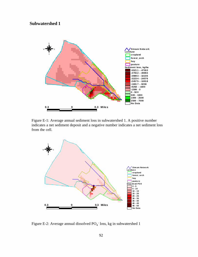
Subwatershed 1
Sediment loss, kg/ha-5521 1 - -47553-4755 2 - -39894-3989 3 - -32235-3223 4 - -24576-2457 5 - -16918-1691 7 - -9259-9258 - -1600-1599 - 00 - 50 0500 - 10001000 - 25002500 - 7000No Data
Landusecropland
fo rest_orchhaypasture
Stream N etw ork
0.3 0 0.3 Mile s
N
EW
S
Figure E-1: Average annual sediment loss in subwatershed 1. A positive number indicates a net sediment deposit and a negative number indicates a net sediment loss from the cell.
Diss olv ed PO40 - 55 - 1010 - 1515 - 2020 - 2530 - 3535 - 4040 - 4545 - 50No Data
La ndus ecrop landforest_orchhaypastu re
Stre am Network
0.3 0 0.3 Miles
N
EW
S
Figure E-2: Average annual dissolved PO4- loss, kg in subwatershed 1
92

Sediment-bound NH4, kg0 - 2.0272.027 - 4.0534.053 - 6.086.08 - 8 .1078.107 - 10.13310.133 - 12.1612.16 - 14.18714.187 - 16.21316.213 - 18.24No Data
Landusecroplandforest_orchhaypasture
Stream Network
0.3 0 0.3 Miles
N
EW
S
Figure E-3: Average annual sediment-bound NH4+ loss in kg, in subwatershed 1
Dssolved NO3, kg0 - 1.3131.3 13 - 2 .62 62.6 26 - 3 .93 93.9 39 - 5 .25 25.2 52 - 6 .56 66.5 66 - 7 .87 97.8 79 - 9 .19 29.1 92 - 1 0.5 0510.505 - 11.818No Dat a
Landusecropla ndforest _orchhaypasture
Stream Network
0.3 0 0.3 Miles
N
EW
S
Figure E-4: Average annual dissolved NO3 loss in kg, in subwatershed 1
93

Subwatershed 2
Figure E-5: Average annual sediment loss in subwatershed 2. A positive number indicates a net sediment deposit and a negative number indicates a net sediment loss from the cell.
Diss olved PO4, kg0 - 55 - 1010 - 1515 - 2020 - 2525 - 5050 - 100100 - 125125 - 150150 - 175175 - 200No D ata
Landusecroplandfores t_ orchha ypa sture
Stream
0.6 0 0.6 Miles
N
EW
S
Figure E-6: Average annual dissolved PO4- loss in kg, in subwatershed 2
Sediment loss, kg/ha-120966 - -103962-103962 - -86958-86958 - -69953-69953 - -52949-52949 - -35945-35945 - -18941-18941 - -1936-1936 - 00 - 3207 232072 - 4907 649076 - 6608 066080 - 8308 483084 - 1000 88100088 - 117 093117093 - 134 097134097 - 151 101No Data
La ndusecrop landforest_orch
haypasture
Stream
0.6 0 0.6 Mile s
N
EW
S
94

Se diment NH4, kg0 - 2.52.5 - 5.55.5 - 10.510.5 - 20.520.5 - 30.530.5 - 40.540.5 - 50.550.5 - 60.560.5 - 70.570.5 - 8181 - 91No Data
Landusecropland
for es t_ orchhay
pasture
Stream
0.6 0 0.6 Miles
N
EW
S
Figure E-7: Average annual sediment-bound NH4+ loss in kg, in subwatershed 2
Dissolved NO3, kg0 - 2.9832.9 83 - 4.9664.9 66 - 8.9498.9 49 - 14.93214.932 - 24.91624.916 - 29.89929.899 - 34.88234.882 - 39.86539.865 - 44.848No Data
Landusecroplandforest_orchhay
pasture
Stream
0.6 0 0.6 Miles
N
EW
S
Figure E-8 Average annual dissolved NO3 loss in kg, in subwatershed 2
95

Subwatershed 3
Sediment loss, kg/ha-79738 - -61228-612278 - -42718-42718 - -24208-24208 - -5698-5698 - 00 - 10001000 - 1000010000 - 2000020000 - 3000030000 - 90000No Data
Landusecroplandforest_ orchhaypasture
Stream Network
0.3 0 0.3 Mi le s
N
EW
S
Figure E-9: Average annual sediment loss in subwatershed 3. A positive number indicates a net sediment deposit and a negative number indicates a net sediment loss from the cell.
Figure E-10: Average annual dissolved PO4- loss in kg, in subwatershed 3
Dissolved PO4, kg0.021 - 34.55534.555 - 69.08969.089 - 103.623103.623 - 138.157138.157 - 172.691172.691 - 207.225207.225 - 241.759241.759 - 276.293276.293 - 310.827No Data
Landusecroplandforest_orchhaypasture
Stream Network
0.3 0 0.3 Miles
N
EW
S
96

Figure E-11: Average annual sediment-bound NH4+ loss in kg, in subwatershed 3
Figure E-12 Average annual dissolved NO3 loss in kg, in subwatershed 3
Se dim ent-NH 4, kg0.0 01 - 13 .22613 .226 - 2 6.45 226 .452 - 3 9.67 739 .677 - 5 2.90 352 .903 - 6 6.12 866 .128 - 7 9.35 479 .354 - 9 2.57 992 .579 - 1 05 .8 0510 5.80 5 - 11 9.03No Da ta
La ndusecroplan dfore st_ orchha ypa sture
Strea m N etwork
0.3 0 0.3 Miles
N
EW
S
Dis solved NO3, k g0.053 - 4 .9 534.953 - 9 .8 539.853 - 1 4.75314.753 - 19.65 319.653 - 24.55 224.552 - 29.45 229.452 - 34.35 234.352 - 39.25 239.252 - 44.15 2No Da ta
Landusecroplandfore st_orchhaypasture
Stream Network
0.3 0 0.3 Mile s
N
EW
S
97

Subwatershed 4
Figure E-13: Average annual sediment loss in subwatershed 4. A positive number indicates a net sediment deposit and a negative number indicates a net sediment loss from the cell.
Figure E-14: Average annual dissolved PO4- loss in kg, in subwatershed 4
Se dimen t los s, kg/ha-24 607 44 - -1 964 58 5-19 645 85 - -1 468 42 6-14 684 26 - -9 722 66-97 226 6 - -47 610 6-47 610 6 - -20 000-20 000 - -100 00-10 000 - 00 - 200 53.2 2 220 05 3.2 22 - 51 6 21 2.66 751 62 12. 667 - 1 0 12 372 .11110 12 372 .11 1 - 1 50 853 1.55 615 08 531 .55 6 - 2 00 469 1No Data
La ndusecro pla nd
fore st_o rch
ha y
pa sture
Stre am Network
0.3 0 0.3 Mile s
N
EW
S
Dis solve d PO 4, k g0 - 1000 - 50050 0 - 1 50015 00 - 396 839 68 - 793 5. 98 579 35 .9 8 5 - 1 19 0 3.97 311 90 3.9 73 - 15 8 71 .9 6215 87 1.9 62 - 19 8 39 .9 5119 83 9.9 51 - 23 8 07 .9 423 80 7.9 4 - 2 77 7 5.92 927 77 5.9 29 - 31 7 43 .9 1731 74 3.9 17 - 35 7 11 .9 06No Data
La ndusecro pla nd
fore st_o rch
ha y
pa sture
Stre am Network
0.3 0 0.3 Mile s
N
EW
S
98

Figure E-15: Average annual sediment-bound NH4+ loss in kg, in subwatershed 4
Figure E-16 Average annual dissolved NO3 loss in subwatershed 4
Sediment-N H4, kg0 - 100100 - 4535.2244535.224 - 9070.4479070.447 - 13605.67113605.671 - 18140.89418140.894 - 22676.11822676.118 - 27211.34127211.341 - 31746.56531746.565 - 36281.78836281.788 - 40817.012No Data
Landu secrop landforest_orchhaypastu re
Stream N etwork
0.3 0 0.3 Miles
N
EW
S
99
Dissolved N O3, kg0 - 553.587553.587 - 1107.1751107.175 - 1660.7621660.762 - 2214.3492214.349 - 2767.9372767.937 - 3321.5243321.524 - 3875.1113875.111 - 4428.6994428.699 - 4982.286No Data
Landusecroplandforest_orchhay
pasture
Stream Network
0.3 0 0.3 Miles
N
EW
S

Subwatershed 5
Figure E-17: Average annual sediment loss in subwatershed 5. A positive number indicates a net sediment deposit and a negative number indicates a net sediment loss from the cell.
Figure E-18: Average annual dissolved PO4- loss in kg, in subwatershed 5
Sed iment loss, kg/ha-85000 - -65000-65000 - -45000-45000 - -30000-30000 - -15000-15000 - -5000-5000 - -500-500 - 00 - 10001000 - 1000010000 - 2000020000 - 3000030000 - 40000No Data
Stream Network
Landu secroplandforest_orchhaypasture
0.3 0 0.3 Miles
N
EW
S
Disso lved PO4, kg0.005 - 21.83221.832 - 43.6643.66 - 65.48765.487 - 87.31487.314 - 109.142109.142 - 130.969130.969 - 152.796152.796 - 174.624174.624 - 196.451No Data
Stream Netwo rk
Landusecroplandforest_orchhaypastu re
0.3 0 0.3 Miles
N
EW
S
100

Figure E-19: Average annual sediment-bound NH4+ loss in kg, in subwatershed 5
Figure E-20 Average annual dissolved NO3 loss in kg, in subwatershed 5
Sediment-N H4, kg0 - 10 .20510.205 - 20.41120.411 - 30.61630.616 - 40.82240.822 - 51.02751.027 - 61.23361.233 - 71.43871.438 - 81.64481.644 - 91.849No Data
Stream Network
Landusecropla ndforest_orchhaypasture
0.3 0 0.3 Mile s
N
EW
S
Dissolved NO3, kg0 - 3.1443.144 - 6.2886.288 - 9.4319.431 - 12.57512.575 - 15.71915.719 - 18.86318.863 - 22.00622.006 - 25.1525.15 - 28.294No Data
Stream Network
Landusecropla ndforest_orchhaypasture
0.3 0 0.3 Miles
N
EW
S
101

Subwatershed 6
Figure E-21: Average annual sediment loss in subwatershed 6. A positive number indicates a net sediment deposit and a negative number indicates a net sediment loss from the cell.
Figure E-22: Average annual dissolved PO4- loss in kg, in subwatershed 6
Sediment loss, kg/ha-43000 - -34000-34000 - -24000-24000 - -14000-14000 - -4000-4000 - -2000-2000 - -1000-1000 - 00 - 500500 - 15001500 - 1500015000 - 30000No Data
Landusecroplandforest_orchhaypasture
Stream Network
0.4 0 0.4 Miles
N
EW
S
Dis so lve d -PO4 , kg0 - 3 .0 723.0 7 2 - 6 .1446.1 4 4 - 9 .2159.2 1 5 - 1 2.28 712.2 87 - 15.3 5915.3 59 - 18.4 3118.4 31 - 21.5 0221.5 02 - 24.5 7424.5 74 - 27.6 46No Da ta
La ndusecroplandfore s t_ orc hha ypa sture
Stre am Netw ork
0.4 0 0.4 Miles
N
EW
S
102

Figure E-23: Average annual sediment-bound NH4+ loss in subwatershed 6
Figure E-24 Average annual dissolved NO3 loss in subwatershed 6
Sediment -NH 4, kg0 - 1 .0261.026 - 2.0522.052 - 3.0783.078 - 4.1044.104 - 5.135.13 - 6.1566.156 - 7.1827.182 - 8.2088.208 - 9.234No Da ta
Landusecroplandforest_orchhaypasture
Stream Network
0.4 0 0.4 Miles
N
EW
S
103
Dissolved NO3, kg0 - 0.6330.633 - 1.2661.266 - 1.8991.899 - 2.5322.532 - 3.1653.165 - 3.7983.798 - 4.4314.431 - 5.0645.064 - 5.697No Data
Landusecroplandforest_orchhaypasture
Stream Network
0.4 0 0.4 Miles
N
EW
S

Subwatershed 7
Figure E-25: Average annual sediment loss in subwatershed 7. A positive number indicates a net sediment deposit and a negative number indicates a net sediment loss from the cell.
Figure E-26: Average annual dissolved PO4- loss in kg, in subwatershed 7
Sedime nt los s, kg/ha-31 89 2 - -281 29-28 12 9 - -243 66-24 36 6 - -206 03-20 60 3 - -168 40-16 84 0 - -130 77-13 07 7 - -931 4-93 14 - -5 551-55 51 - -1 788-17 88 - -5 00-50 0 - 00 - 10 0100 - 500500 - 2000No Da ta
Landus ecrop la ndforest_ orchhaypasture
Stream Network
0.3 0 0.3 Miles
N
EW
S
Dissolved PO4, kg0.059 - 50.98250.982 - 101.904101.904 - 152.827152.827 - 203.749203.749 - 254.672254.672 - 305.594305.594 - 356.517356.517 - 407.439407.439 - 458.362No Data
Landusecroplandforest_orchhaypasture
Stream Network
0.3 0 0.3 Miles
N
EW
S
104
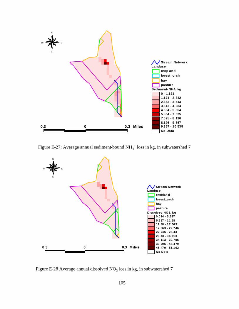
Figure E-27: Average annual sediment-bound NH4+ loss in kg, in subwatershed 7
Figure E-28 Average annual dissolved NO3 loss in kg, in subwatershed 7
Diss olv ed NO3, k g0.0 14 - 5 .6 975.6 97 - 1 1.3811.38 - 1 7.06 317.06 3 - 22.7 4622.74 6 - 28.4 328.43 - 3 4.11 334.11 3 - 39.7 9639.79 6 - 45.4 7945.47 9 - 51.1 62No Da ta
Landus ecroplan d
fo rest_orchhaypasture
Stream Network
0.3 0 0.3 Miles
N
EW
S
105
Sediment-NH4, kg0 - 1.1711.171 - 2.3422.342 - 3.5133.513 - 4.6844.684 - 5.8545.854 - 7.0257.025 - 8.1968.196 - 9.3679.367 - 10.538No Data
Landusecroplandforest_orch
haypasture
Stream Network
0.3 0 0.3 Miles
N
EW
S

Subwatershed 8
Figure E-29 Average annual sediment loss in subwatershed 8. A positive number indicates a net sediment deposit and a negative number indicates a net sediment loss from the cell.
Figure E-30: Average annual dissolved PO4- loss in kg, in subwatershed 8
Sediment loss, kg/ha-56298 - -35292-35291 - -25000-25000 - -15000-15000 - -10000-10000 - -5000-5000 - -2500-2500 - -1000-1000 - 00 - 10001000 - 2000020000 - 111756111756 - 132762No Data
Landusecroplandforest_orchhaypasture
Stream Network
0.3 0 0.3 Miles
N
EW
S
Dissolved PO4, kg0.135 - 14.17614.176 - 28.21728.217 - 42.25842.258 - 56.29956.299 - 70.3470.34 - 84.38184.381 - 98.42298.422 - 112.463112.463 - 126.504No Data
Landusecroplandforest_orchhaypasture
Stream Network
0.3 0 0.3 Miles
N
EW
S
106
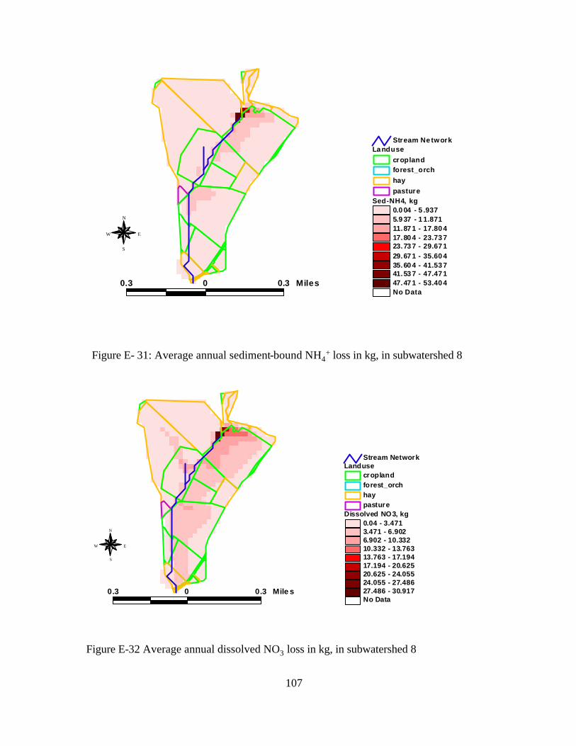
Figure E- 31: Average annual sediment-bound NH4+ loss in kg, in subwatershed 8
Figure E-32 Average annual dissolved NO3 loss in kg, in subwatershed 8
Sed-NH4, kg0.0 04 - 5 .9375.9 37 - 1 1.87111.87 1 - 17.80 417.80 4 - 23.73 723.73 7 - 29.67 129.67 1 - 35.60 435.60 4 - 41.53 741.53 7 - 47.47 147.47 1 - 53.40 4No Data
La ndusecroplandforest_orchhaypasture
Stream Ne twork
0.3 0 0.3 Miles
N
EW
S
Dissolved NO3, kg0.04 - 3.4713.471 - 6.9026.902 - 10.33210.332 - 13.76313.763 - 17.19417.194 - 20.62520.625 - 24.05524.055 - 27.48627.486 - 30.917No Data
Landusecroplandforest_orchhaypasture
Stream Network
0.3 0 0.3 Mile s
N
EW
S
107
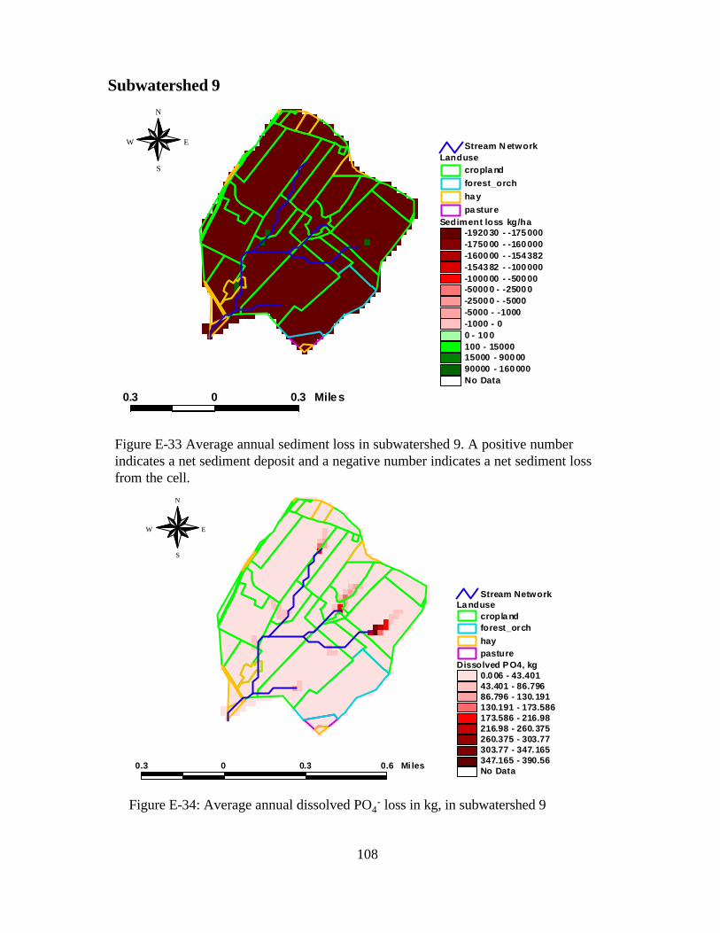
Subwatershed 9
Figure E-33 Average annual sediment loss in subwatershed 9. A positive number indicates a net sediment deposit and a negative number indicates a net sediment loss from the cell.
Figure E-34: Average annual dissolved PO4- loss in kg, in subwatershed 9
Sediment loss kg/ha-1920 30 - -175 000-1750 00 - -160 000-1600 00 - -154 382-1543 82 - -100 000-1000 00 - -500 00-5000 0 - -2500 0-2500 0 - -5000-5000 - -1000-1000 - 00 - 10 0100 - 1500015000 - 900 0090000 - 160 000No Data
Landusecropla ndforest_orchha ypa sture
Stream N etwork
0.3 0 0.3 Miles
N
EW
S
108
Dissolved PO4, kg0.0 06 - 43.40143.401 - 86.79686.796 - 130.191130.191 - 173.586173.586 - 216.98216.98 - 260.375260.375 - 303.77303.77 - 347.165347.165 - 390.56No Data
La ndusecropla ndforest_orchhaypasture
Stream Network
0.3 0 0.3 0.6 Mi les
N
EW
S

Figure E 35-: Average annual sediment-bound NH4+ loss in kg, in subwatershed 9
Figure E-36 Average annual dissolved NO3 loss in kg, in subwatershed 9
Sedim ent-NH4, kg0 - 22.722.7 - 45.40145.401 - 68.10168.101 - 90.80290.802 - 113.502113.502 - 136.203136.203 - 158.903158.903 - 181.604181.604 - 204.304No Data
Landusecroplandforest_orchhaypastu re
Stream Network
0.3 0 0.3 Miles
N
EW
S
Dissolved NO3, kg0 - 12.10412.104 - 24.20924.209 - 36.31336.313 - 48.41748.417 - 60.52260.522 - 72.62672.626 - 84.7384.73 - 96.83596.835 - 108.939No Data
Landusecroplandforest_ orchhaypasture
Stream Network
0.3 0 0.3 Miles
N
EW
S
109

watersh ed.shp
Sedime nt, kg/ha-15790 1 - -13 7822.533-13782 2.5 33 - -1 17744 .0 67-11774 4.0 67 - -9 7665.6-97665 .6 - -7758 7.1 33-77587 .13 3 - -57 508.667-57508 .66 7 - -37 430.2-37430 .2 - -1735 1.7 33-17351 .73 3 - 00 - 100 0100 0 - 10000100 00 - 2000 0200 00 - 3000 0300 00 - 4000 0400 00 - 5000 0500 00 - 1000 00100 000 - 150 000No Data
Stream Netwo rk (100)
Landus ecroplandfores t_orchhaypasture
0.4 0 0.4 Miles
N
EW
S
Figure E-37: Average annual sediment loss in subwatershed 10. A positive number indicates a net sediment deposit and a negative number indicates a net sediment loss from the cell.
Figure E-38: Average annual dissolved PO4- loss in kg, in subwatershed 10
Subwatershed 10
110
Di ssolved PO4, kg0 - 19. 34819.348 - 38.69638.696 - 58.04458.044 - 77.39277.392 - 96.7496.74 - 116.088116.088 - 135.436135.436 - 154.784154.784 - 174.132No Data
Landu secropland
forest_orch
haypasture
Stream Network
0.4 0 0.4 0.8 Miles
N
EW
S

Sed-nh4, kg0 - 1010 - 2 020 - 3 030 - 4 040 - 5 050 - 6 060 - 7 070 - 8 080 - 9 090 - 1 00No Data
St ream
La ndusecropla ndforest _orchha ypa sture
0.4 0 0.4 Miles
N
EW
S
Figure A-39: Average annual sediment-bound NH4+ loss in kg, in subwatershed 10
Figure A-40: Average annual dissolved NO3 loss in kg, in subwatershed 10
111
Dissolved NO3, kg0 - 6.56.5 - 1313 - 2 626 - 3 333 - 3 838 - 4 242 - 4 545 - 5 050 - 6 0No Data
La ndusecroplandforest_orchhaypasture
Stream Network
0.4 0 0.4 0.8 Miles
N
EW
S

Subwatershed 11
Figure E-41: Average annual sediment loss in subwatershed 11. A positive number indicates a net sediment deposit and a negative number indicates a net sediment loss from the cell.
Figure E-42: Average annual dissolved PO4- loss in kg, in subwatershed 11
Sediment los s, kg/ha-162119 - -144107-144106 - -126094-126093 - -108081-108080 - -90068-90067 - -72055-72054 - -54042-54041 - -36029-36028 - -18016-18016 - -5000-5000 - -1000-1000 - 00 - 100No Data
Landusecrop landforest_orchhaypasture
Strea m Network
0.3 0 0.3 Miles
N
EW
S
Dissolved PO4, kg0.084 - 26.45226.452 - 52.82152.821 - 79.18979.189 - 105.558105.558 - 131.926131.926 - 158.295158.295 - 184.663184.663 - 211.032211.032 - 237.4No Data
Landusecrop landforest_orchhaypasture
Stream Network
0.3 0 0.3 Miles
N
EW
S
112

Figure E-43: Average annual sediment-bound NH4+ loss in kg, in subwatershed 11
Figure E-44: Average annual dissolved NO3 loss in kg, in subwatershed 11
Sediment NH4, kg0. 003 - 12.38712.387 - 24.7724.77 - 37.15437.154 - 49.53749.537 - 61.92161.921 - 74.30474.304 - 86.68886.688 - 99.07199.071 - 111.455No Data
Landu secrop land
forest_orch
hay
pasture
Stream Network
0.3 0 0.3 Miles
N
EW
S
Disso lved NO3, kg0.182 - 6.656.65 - 13.11813 .118 - 19.58619 .586 - 26.05426 .054 - 32.52332 .523 - 38.99138 .991 - 45.45945 .459 - 51.92751 .927 - 58.395No D ata
La ndusecrop landforest_orch
haypastu re
Stream N etwork
0.3 0 0.3 Miles
N
EW
S
113

Subwatershed 12
Figure E-45: Average annual sediment loss in subwatershed 12. A positive number indicates a net sediment deposit and a negative number indicates a net sediment loss from the cell.
Figure E-46: Average annual dissolved PO4- loss in kg,in subwatershed 12
Sed iment loss, kg/ha-153034 - -120000-120000 - -90000-90000 - -60000-60000 - -30000-30000 - -15000-15000 - -5000-5000 - -1000-1000 - 00 - 10001000 - 100000100000 - 200000200000 - 300000300000 - 400000400000 - 500000No Data
Landu secroplandforest_orch
hay
pasture
Stream Network
0.4 0 0.4 Miles
N
EW
S
Dissolved PO4, kg0.12 - 56.76156.761 - 113.403113.403 - 170.044170.044 - 226.685226.685 - 283.327283.327 - 339.968339.968 - 396.609396.609 - 453.251453.251 - 509.892No Data
Landusecropland
forest_orchhay
pasture
Stream Netw ork
0.4 0 0.4 Miles
N
EW
S
114

Figure E-47: Average annual sediment-bound NH4+ loss in kg, in subwatershed 12
Figure E-48: Average annual dissolved NO3 loss in kg, in subwatershed 12
Sediment NH4, kg0 - 14 .18614.186 - 28.37328.373 - 42.55942.559 - 56.74556.745 - 70.93270.932 - 85.11885.118 - 99.30499.304 - 113.491113.491 - 127.677No Data
La ndusecropla ndforest_orchha ypa sture
Stream Network
0.4 0 0.4 Miles
N
EW
S
Dissolved NO3, kg0.0 45 - 6.7666.7 66 - 13.48813.488 - 20.20920.209 - 26.93126.931 - 33.65233.652 - 40.37440.374 - 47.09547.095 - 53.81753.817 - 60.538No Data
Landusecropla ndforest_orchhaypasture
Stream Network
0.4 0 0.4 Miles
N
EW
S
115

Tone Merete Nordberg Appendix F BSE
116
APPENDIX F: F-tables calculations

Tone Merete Nordberg Appendix F BSE
117
Figure F.1: Cross sectional diagram of stream used for F-tables. The following equations were used to develop the F-tables for HSPF.
( )( )aTandTp ×= [F.1] Where: Tp = top triangular width (figure F.1) (m); and a = side slope angle (degrees).
( )
==aCos
dWettedSideSw _ [F.2]
Where: Sw =side wetted length (m);
d = depth of water; and a = side slope angle (degrees).
SbSwWp +×= 2 [F.3] Where: Wp = wetted perimeter, (m); Sw = side wetted length (m); and Sb = stream bottom width (m).

Tone Merete Nordberg Appendix F BSE
118
WpA
Rh = [F.4]
Where: Rh = hydraulic radius (m); A = cross sectional area of stream (m2); and Wp = wetted perimeter (m).
( ) 21
32
1SRh
nV ××= [F.5]
Where: V = flow velocity (m/s); n = Manning roughness coefficient; and S = slope in direction of flow (m/m).
TpSbWs ×+= 2 [F.6] Where: Ws = water surface width (m); Sb = bottom stream width (m); and Tp = top triangular width (m).
( ) 000,10WsLArea ×= [F.7] Where: Area = surface area of stream, (ha); L = length of stream (m); and Ws = water surface width (m).
LAVolume ×= [F.8] Where: Volume = volume of water in stream (m3); L = length of stream (m); and A = cross sectional area (m2).
VAOutflow ×= [F.9] Where: Outflow = flow rate (m3/s); V = flow velocity, (m/s); and A = cross sectional area (m2).
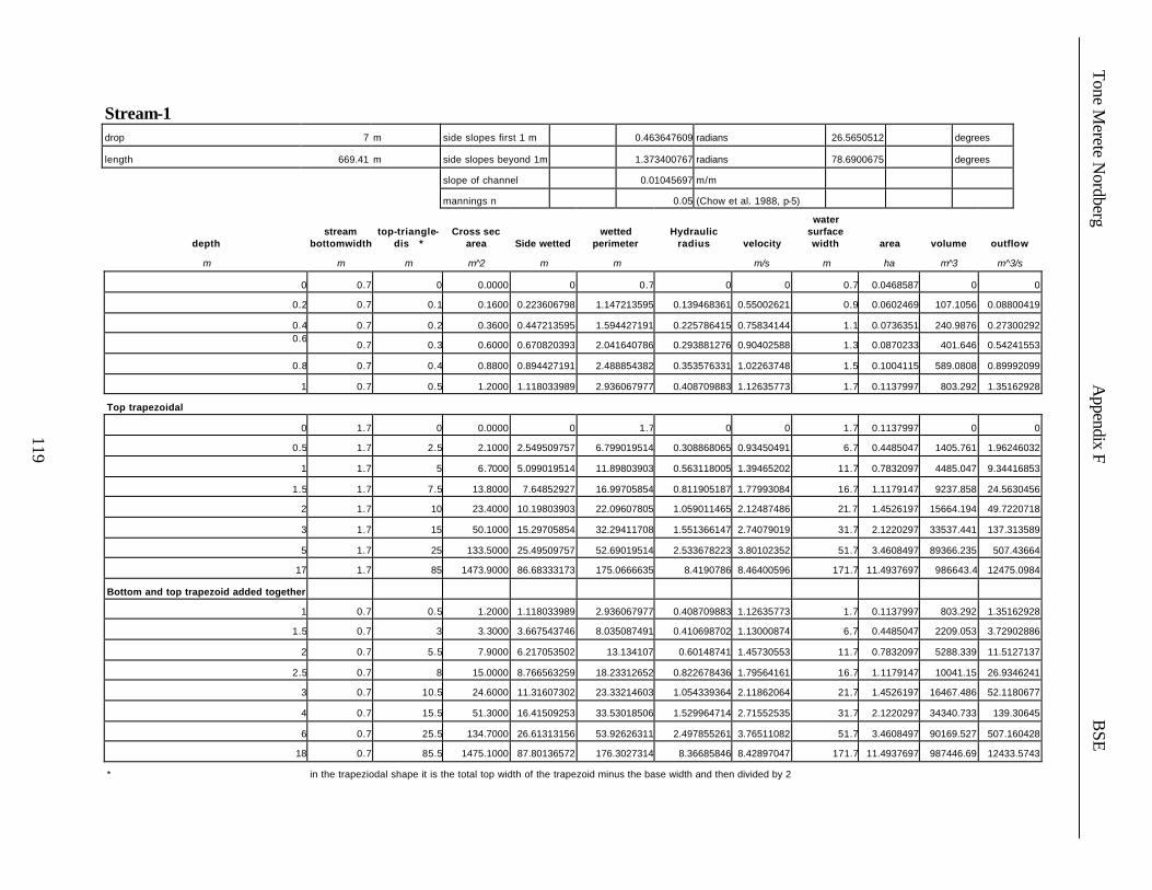
Stream-1 drop 7 m side slopes first 1 m 0.463647609 radians 26.5650512 degrees
length 669.41 m side slopes beyond 1m 1.373400767 radians 78.6900675 degrees
slope of channel 0.01045697 m/m
mannings n 0.05 (Chow et al. 1988, p-5)
depth stream
bottomwidth top-triangle-
dis * Cross sec
area Side wetted wetted
perimeter Hydraulic
radius velocity
water surface width area volume outflow
m m m m^2 m m m/s m ha m^3 m^3/s
0 0.7 0 0.0000 0 0.7 0 0 0.7 0.0468587 0 0
0.2 0.7 0.1 0.1600 0.223606798 1.147213595 0.139468361 0.55002621 0.9 0.0602469 107.1056 0.08800419
0.4 0.7 0.2 0.3600 0.447213595 1.594427191 0.225786415 0.75834144 1.1 0.0736351 240.9876 0.27300292 0.6
0.7 0.3 0.6000 0.670820393 2.041640786 0.293881276 0.90402588 1.3 0.0870233 401.646 0.54241553
0.8 0.7 0.4 0.8800 0.894427191 2.488854382 0.353576331 1.02263748 1.5 0.1004115 589.0808 0.89992099
1 0.7 0.5 1.2000 1.118033989 2.936067977 0.408709883 1.12635773 1.7 0.1137997 803.292 1.35162928
Top trapezoidal
0 1.7 0 0.0000 0 1.7 0 0 1.7 0.1137997 0 0
0.5 1.7 2.5 2.1000 2.549509757 6.799019514 0.308868065 0.93450491 6.7 0.4485047 1405.761 1.96246032
1 1.7 5 6.7000 5.099019514 11.89803903 0.563118005 1.39465202 11.7 0.7832097 4485.047 9.34416853
1.5 1.7 7.5 13.8000 7.64852927 16.99705854 0.811905187 1.77993084 16.7 1.1179147 9237.858 24.5630456
2 1.7 10 23.4000 10.19803903 22.09607805 1.059011465 2.12487486 21.7 1.4526197 15664.194 49.7220718
3 1.7 15 50.1000 15.29705854 32.29411708 1.551366147 2.74079019 31.7 2.1220297 33537.441 137.313589
5 1.7 25 133.5000 25.49509757 52.69019514 2.533678223 3.80102352 51.7 3.4608497 89366.235 507.43664
17 1.7 85 1473.9000 86.68333173 175.0666635 8.4190786 8.46400596 171.7 11.4937697 986643.4 12475.0984
Bottom and top trapezoid added together
1 0.7 0.5 1.2000 1.118033989 2.936067977 0.408709883 1.12635773 1.7 0.1137997 803.292 1.35162928
1.5 0.7 3 3.3000 3.667543746 8.035087491 0.410698702 1.13000874 6.7 0.4485047 2209.053 3.72902886
2 0.7 5.5 7.9000 6.217053502 13.134107 0.60148741 1.45730553 11.7 0.7832097 5288.339 11.5127137
2.5 0.7 8 15.0000 8.766563259 18.23312652 0.822678436 1.79564161 16.7 1.1179147 10041.15 26.9346241
3 0.7 10.5 24.6000 11.31607302 23.33214603 1.054339364 2.11862064 21.7 1.4526197 16467.486 52.1180677
4 0.7 15.5 51.3000 16.41509253 33.53018506 1.529964714 2.71552535 31.7 2.1220297 34340.733 139.30645
6 0.7 25.5 134.7000 26.61313156 53.92626311 2.497855261 3.76511082 51.7 3.4608497 90169.527 507.160428
18 0.7 85.5 1475.1000 87.80136572 176.3027314 8.36685846 8.42897047 171.7 11.4937697 987446.69 12433.5743
* in the trapeziodal shape it is the total top width of the trapezoid minus the base width and then divided by 2
Tone M
erete Nordberg
A
ppendix F
BSE
119

Stream-2 drop 7 m side slopes first 1 m 0.463647609 radians 26.56505118 degrees
length 1151.54 m side slopes beyond 1m 1.373400767 radians 78.69006753 degrees
slope of channel 0.006078816 m/m
mannings n 0.05 (Chow et al. 1988, p-5)
depth stream
bottomwidth top-triangle-
dis * Cross sec area Side wetted wetted
perimeter Hydraulic
radius velocity
water surface width area volume outflow
m m m m^2 m m m/s m ha m̂ 3 m^3/s
0 1 0 0.0000 0 1 0 0 1 0.115154 0 0
0.2 1 0.1 0.2200 0.223606798 1.447213595 0.152016261 0.444153272 1.2 0.1381848 253.3388 0.09771372
0.4 1 0.2 0.4800 0.447213595 1.894427191 0.253374742 0.624379134 1.4 0.1612156 552.7392 0.299701984
0.6 1 0.3 0.7800 0.670820393 2.341640786 0.333099767 0.749299979 1.6 0.1842464 898.2012 0.584453984
0.8 1 0.4 1.1200 0.894427191 2.788854382 0.401598594 0.848791375 1.8 0.2072772 1289.7248 0.95064634
1 1 0.5 1.5000 1.118033989 3.236067977 0.463525492 0.933946324 2 0.230308 1727.31 1.400919486
Top trapezoidal
0 2 0 0.0000 0 2 0 0 2 0.230308 0 0
0.5 2 2.5 2.2500 2.549509757 7.099019514 0.316945178 0.724873573 7 0.806078 2590.965 1.63096554
1 2 5 7.0000 5.099019514 12.19803903 0.573862732 1.076824304 12 1.381848 8060.78 7.537770131
1.5 2 7.5 14.2500 7.64852927 17.29705854 0.823839497 1.370359687 17 1.957618 16409.445 19.52762555
2 2 10 24.0000 10.19803903 22.39607805 1.071616197 1.632922906 22 2.533388 27636.96 39.19014973
3 2 15 51.0000 15.29705854 32.59411708 1.56469954 2.101648771 32 3.684928 58728.54 107.1840873
5 2 25 135.0000 25.49509757 52.99019514 2.547641118 2.908696007 52 5.988008 155457.9 392.6739609
17 2 85 1479.0000 86.68333173 175.3666635 8.433757995 6.460809335 172 19.806488 1703127.66 9555.537007
Bottom and top trapezoid added together
1 1 0.5 1.5000 1.118033989 3.236067977 0.463525492 0.933946324 2 0.230308 1727.31 1.400919486
1.5 1 3 3.7500 3.667543746 8.335087491 0.449905295 0.915560199 7 0.806078 4318.275 3.433350746
2 1 5.5 8.5000 6.217053502 13.434107 0.632717902 1.149245777 12 1.381848 9788.09 9.768589104
2.5 1 8 15.7500 8.766563259 18.53312652 0.849829627 1.399031243 17 1.957618 18136.755 22.03474208
3 1 10.5 25.5000 11.31607302 23.63214603 1.079038694 1.640454468 22 2.533388 29364.27 41.83158893
4 1 15.5 52.5000 16.41509253 33.83018506 1.551868543 2.090143585 32 3.684928 60455.85 109.7325382
6 1 25.5 136.5000 26.61313156 54.22626311 2.517230437 2.885502696 52 5.988008 157185.21 393.871118
18 1 85.5 1480.5000 87.80136572 176.6027314 8.383222547 6.434974523 172 19.806488 1704854.97 9526.979781
* in the trapeziodal shape it is the total top width of the trapezoid minus the base width and then divided by 2
Tone M
erete Nordberg
A
ppendix F
BSE
120

Stream 3 drop 6 m side slopes first 1 m 0.463647609 radians 26.56505118 degrees
length 814.26 m side slopes beyond 1m 1.373400767 radians 78.69006753 degrees
slope of channel 0.007368654 m/m
mannings n 0.05 (Chow et al. 1988, p-5)
depth stream
bottmwidth
top-triangle-dis
* Cross sec
area Side
wetted wetted perimeter Hydraulic radius velocity
water surface width area volume outflow
m m m m^2 m m m/s m ha m^3 m^3/s
0 0.7 0 0.0000 0 0.7 0 0 0.7 0.0569982 0 0
0.2 0.7 0.1 0.1600 0.2236068 1.147213595 0.139468361 0.461715586 0.9 0.0732834 130.2816 0.073874494
0.4 0.7 0.2 0.3600 0.4472136 1.594427191 0.225786415 0.636584328 1.1 0.0895686 293.1336 0.229170358
0.6 0.7 0.3 0.6000 0.67082039 2.041640786 0.293881276 0.758878092 1.3 0.1058538 488.556 0.455326855
0.8 0.7 0.4 0.8800 0.89442719 2.488854382 0.353576331 0.85844576 1.5 0.122139 716.5488 0.755432269
1 0.7 0.5 1.2000 1.11803399 2.936067977 0.408709883 0.945512984 1.7 0.1384242 977.112 1.13461558
Top trapezoidal
0 1.7 0 0.0000 0 1.7 0 0 1.7 0.1384242 0 0
0.5 1.7 2.5 2.1000 2.54950976 6.799019514 0.308868065 0.784463501 6.7 0.5455542 1709.946 1.647373352
1 1.7 5 6.7000 5.09901951 11.89803903 0.563118005 1.170730716 11.7 0.9526842 5455.542 7.843895795
1.5 1.7 7.5 13.8000 7.64852927 16.99705854 0.811905187 1.494150282 16.7 1.3598142 11236.788 20.6192739
2 1.7 10 23.4000 10.198039 22.09607805 1.059011465 1.783711087 21.7 1.7669442 19053.684 41.73883944
3 1.7 15 50.1000 15.2970585 32.29411708 1.551366147 2.300736826 31.7 2.5812042 40794.426 115.266915
5 1.7 25 133.5000 25.4950976 52.69019514 2.533678223 3.190742151 51.7 4.2097242 108703.71 425.9640772
17 1.7 85 1473.9000 86.6833317 175.0666635 8.4190786 7.105049585 171.7 13.9808442 1200137.814 10472.13258
Bottom and top trapezoid added together
1 0.7 0.5 1.2000 1.11803399 2.936067977 0.408709883 0.945512984 1.7 0.1384242 977.112 1.13461558
1.5 0.7 3 3.3000 3.66754375 8.035087491 0.410698702 0.948577801 6.7 0.5455542 2687.058 3.130306744
2 0.7 5.5 7.9000 6.2170535 13.134107 0.60148741 1.223324756 11.7 0.9526842 6432.654 9.664265572
2.5 0.7 8 15.0000 8.76656326 18.23312652 0.822678436 1.507338572 16.7 1.3598142 12213.9 22.61007859
3 0.7 10.5 24.6000 11.316073 23.33214603 1.054339364 1.778461021 21.7 1.7669442 20030.796 43.75014113
4 0.7 15.5 51.3000 16.4150925 33.53018506 1.529964714 2.279528433 31.7 2.5812042 41771.538 116.9398086
6 0.7 25.5 134.7000 26.6131316 53.92626311 2.497855261 3.160595494 51.7 4.2097242 109680.822 425.7322131
18 0.7 85.5 1475.1000 87.8013657 176.3027314 8.36685846 7.075639296 171.7 13.9808442 1201114.926 10437.27553
* in the trapeziodal shape it is the total top width of the trapezoid minus the base width and then divided by 2
Tone M
erete Nordberg
A
ppendix F
BSE
121

Stream 4 drop 2 m side slopes first 1 m 0.46364761 radians 26.56505118 degrees
length 144.85 m side slopes beyond 1m 1.37340077 radians 78.69006753 degrees
slope of channel 0.01380739 m/m
mannings n 0.05 (Chow et al. 1988, p-5)
depth stream
bottomwidth top-triangle-dis
* Cross sec
area Side wetted wetted
perimeter Hydraulic
radius velocity
water surface width area volume outflow
m m m m^2 m m m/s m ha m^3 m^3/s
0 1.3 0 0.0000 0 1.3 0 0 1.3 0.0188305 0 0
0.2 1.3 0.1 0.2800 0.223606798 1.7472136 0.16025516 0.69336263 1.5 0.0217275 40.558 0.194141536 0.4
1.3 0.2 0.6000 0.447213595 2.19442719 0.27341987 0.990008963 1.7 0.0246245 86.91 0.594005378
0.6 1.3 0.3 0.9600 0.670820393 2.64164079 0.3634105 1.196788456 1.9 0.0275215 139.056 1.148916918
0.8 1.3 0.4 1.3600 0.894427191 3.08885438 0.44029269 1.360128871 2.1 0.0304185 196.996 1.849775265
1 1.3 0.5 1.8000 1.118033989 3.53606798 0.50903999 1.498259397 2.3 0.0333155 260.73 2.696866915
Top trapezoidal
0 2.3 0 0.0000 0 2.3 0 0 2.3 0.0333155 0 0
0.5 2.3 2.5 2.4000 2.549509757 7.39901951 0.3243673 1.109456953 7.3 0.1057405 347.64 2.662696688
1 2.3 5 7.3000 5.099019514 12.498039 0.58409163 1.642125705 12.3 0.1781655 1057.405 11.98751765
1.5 2.3 7.5 14.7000 7.64852927 17.5970585 0.83536689 2.084509671 17.3 0.2505905 2129.295 30.64229216
2 2.3 10 24.6000 10.19803903 22.6960781 1.08388771 2.479754027 22.3 0.3230155 3563.31 61.00194906
3 2.3 15 51.9000 15.29705854 32.8941171 1.57778973 3.185066418 32.3 0.4678655 7517.715 165.3049471
5 2.3 25 136.5000 25.49509757 53.2901951 2.5614468 4.399560602 52.3 0.7575655 19772.025 600.5400222
17 2.3 85 1484.1000 86.68333173 175.666663 8.44838725 9.748436163 172.3 2.4957655 214971.885 14467.65411
Bottom and top trapezoid added together
1 1.3 0.5 1.8000 1.118033989 3.53606798 0.50903999 1.498259397 2.3 0.0333155 260.73 2.696866915
1.5 1.3 3 4.2000 3.667543746 8.63508749 0.48638766 1.453474586 7.3 0.1057405 608.37 6.104593261
2 1.3 5.5 9.1000 6.217053502 13.734107 0.66258403 1.786129955 12.3 0.1781655 1318.135 16.25378259
2.5 1.3 8 16.5000 8.766563259 18.8331265 0.87611582 2.151757988 17.3 0.2505905 2390.025 35.5040068
3 1.3 10.5 26.4000 11.31607302 23.932146 1.10311879 2.508999639 22.3 0.3230155 3824.04 66.23759047
4 1.3 15.5 53.7000 16.41509253 34.1301851 1.57338731 3.179138917 32.3 0.4678655 7778.445 170.7197598
6 1.3 25.5 138.3000 26.61313156 54.5262631 2.53639241 4.370824551 52.3 0.7575655 20032.755 604.4850354
18 1.3 85.5 1485.9000 87.80136572 176.902731 8.39953113 9.710817071 172.3 2.4957655 215232.615 14429.30309
* in the trapeziodal shape it is the total top width of the trapezoid minus the base width and then divided by 2
Tone M
erete Nordberg
A
ppendix F
BSE
122

Stream 5 drop 3 m side slopes first 1 m 0.463647609 radians 26.56505118 degrees
length 429.41 m side slopes beyond 1m 1.373400767 radians 78.69006753 degrees
slope of channel 0.00698633 m/m
mannings n 0.05 (Chow et al. 1988, p-5)
depth stream
bottomwidth
top-triangle-dis * Cross sec area Side wetted
wetted perimeter
Hydraulic radius velocity
water surface width area volume outflow
m m m m^2 m m m/s m ha m^3 m^3/s
0 1.5 0 0.0000 0 1.5 0 0 1.5 0.0644115 0 0
0.2 1.5 0.1 0.3200 0.2236068 1.947213595 0.16433739 0.5015476 1.7 0.0729997 137.4112 0.160495224
0.4 1.5 0.2 0.6800 0.4472136 2.394427191 0.283992766 0.7222586 1.9 0.0815879 291.9988 0.491135858
0.6 1.5 0.3 1.0800 0.67082039 2.841640786 0.380062112 0.8771171 2.1 0.0901761 463.7628 0.947286512
0.8 1.5 0.4 1.5200 0.89442719 3.288854382 0.462167011 0.99928 2.3 0.0987643 652.7032 1.518905528
1 1.5 0.5 2.0000 1.11803399 3.736067977 0.535322165 1.1021263 2.5 0.1073525 858.82 2.204252587
Top trapezoidal
0 2.5 0 0.0000 0 2.5 0 0 2.5 0.1073525 0 0
0.5 2.5 2.5 2.5000 2.54950976 7.599019514 0.328989812 0.7966658 7.5 0.3220575 1073.525 1.991664522
1 2.5 5 7.5000 5.09901951 12.69803903 0.590642381 1.1768044 12.5 0.5367625 3220.575 8.826032995
1.5 2.5 7.5 15.0000 7.64852927 17.79705854 0.842835908 1.4915915 17.5 0.7514675 6441.15 22.37387248
2 2.5 10 25.0000 10.198039 22.89607805 1.091890058 1.7725853 22.5 0.9661725 10735.25 44.31463357
3 2.5 15 52.5000 15.2970585 33.09411708 1.58638467 2.2738416 32.5 1.3955825 22544.025 119.3766862
5 2.5 25 137.5000 25.4950976 53.49019514 2.570564561 3.1369449 52.5 2.2544025 59043.875 431.3299233 17 2.5 85 1487.5000 86.6833317 175.8666635 8.45811236 6.9396385 172.5 7.4073225 638747.375 10322.71223
Bottom and top trapezoid added together
1 1.5 0.5 2.0000 1.11803399 3.736067977 0.535322165 1.1021263 2.5 0.1073525 858.82 2.204252587
1.5 1.5 3 4.5000 3.66754375 8.835087491 0.509332817 1.0661598 7.5 0.3220575 1932.345 4.797719273
2 1.5 5.5 9.5000 6.2170535 13.934107 0.681780325 1.2949436 12.5 0.5367625 4079.395 12.30196425
2.5 1.5 8 17.0000 8.76656326 19.03312652 0.893179583 1.5504118 17.5 0.7514675 7299.97 26.35700094
3 1.5 10.5 27.0000 11.316073 24.13214603 1.118839575 1.8016334 22.5 0.9661725 11594.07 48.64410193
4 1.5 15.5 54.5000 16.4150925 34.33018506 1.587524212 2.2749304 32.5 1.3955825 23402.845 123.9837078
6 1.5 25.5 139.5000 26.6131316 54.72626311 2.549050347 3.1194174 52.5 2.2544025 59902.695 435.1587254
18 1.5 85.5 1489.5000 87.8013657 177.1027314 8.410372827 6.9135012 172.5 7.4073225 639606.195 10297.66009
* in the trapeziodal shape it is the total top width of the trapezoid minus the base width and then divided by 2
Tone M
erete Nordberg
A
ppendix F
BSE
123

Stream 6 drop 15 m side slopes first 1 m 0.463647609 radians 26.56505118
degrees
length 1708.23 m side slopes beyond 1m 1.373400767 radians 78.69006753 degrees
slope of channel 0.008781019 m/m
mannings n 0.05 (Chow et al. 1988, p-5)
depth stream
bottomwidth top-triangle-dis * Cross sec area Side wetted wetted perimeter Hydraulic
radius velocity
water surface width area volume outflow1
m m m m^2 m m m/s m ha m^3 m^3/s
0 2 0 0.0000 0 2 0 0 2 0.341646 0 0
0.2 2 0.1 0.4200 0.2236068 2.447213595 0.17162376 0.5787896 2.2 0.3758106 717.4566 0.243091637
0.4 2 0.2 0.8800 0.4472136 2.894427191 0.304032522 0.8473883 2.4 0.4099752 1503.2424 0.745701735
0.6 2 0.3 1.3800 0.67082039 3.341640786 0.412970779 1.0393185 2.6 0.4441398 2357.3574 1.434259565
0.8 2 0.4 1.9200 0.89442719 3.788854382 0.506749483 1.1912365 2.8 0.4783044 3279.8016 2.287174101
1 2 0.5 2.5000 1.11803399 4.236067977 0.590169944 1.3186226 3 0.512469 4270.575 3.296556474
Top trapezoidal
0 3 0 0.0000 0 3 0 0 3 0.512469 0 00.5
3 2.5 2.7500 2.54950976 8.099019514 0.339547274 0.9121563 8 1.366584 4697.6325 2.508429959
1 3 5 8.0000 5.09901951 13.19803903 0.606150655 1.3423203 13 2.220699 13665.84 10.73856274
1.5 3 7.5 15.7500 7.64852927 18.29705854 0.860794098 1.6959068 18 3.074814 26904.6225 26.71053159
2 3 10 26.0000 10.198039 23.39607805 1.11129737 2.0107403 23 3.928929 44413.98 52.27924717
3 3 15 54.0000 15.2970585 33.59411708 1.607424296 2.5717148 33 5.637159 92244.42 138.8725995
5 3 25 140.0000 25.4950976 53.99019514 2.593063419 3.5373487 53 9.053619 239152.2 495.2288241
17 3 85 1496.0000 86.6833317 176.3666635 8.482328636 7.7949353 173 29.552379 2555512.08 11661.22324
Bottom and top trapezoid added together
1 2 0.5 2.5000 1.11803399 4.236067977 0.590169944 1.3186226 3 0.512469 4270.575 3.296556474
1.5 2 3 5.2500 3.66754375 9.335087491 0.562394301 1.2769181 8 1.366584 8968.2075 6.703820287
2 2 5.5 10.5000 6.2170535 14.434107 0.727443686 1.5158936 13 2.220699 17936.415 15.91688228
2.5 2 8 18.2500 8.76656326 19.53312652 0.934310234 1.7911413 18 3.074814 31175.1975 32.68832938
3 2 10.5 28.5000 11.316073 24.63214603 1.157024644 2.0655269 23 3.928929 48684.555 58.86751717
4 2 15.5 56.5000 16.4150925 34.83018506 1.622156182 2.5874039 33 5.637159 96514.995 146.1883209
6 2 25.5 142.5000 26.6131316 55.22626311 2.580294084 3.5257263 53 9.053619 243422.775 502.4159924
18 2 85.5 1498.5000 87.8013657 177.6027314 8.437370236 7.7673676 173 29.552379 2559782.655 11639.4003
* in the trapeziodal shape it is the total top width of the trapezoid minus the base width and then divided by 2
Tone M
erete Nordberg
A
ppendix E
B
SE
124

Stream 7 drop 1 m side slopes first 1 m 0.463647609 radians 26.56505118 degrees
length 34.06 m side slopes beyond 1m 1.373400767 radians 78.69006753 degrees
slope of channel 0.029359953 m/m
mannings n 0.05 (Chow et al. 1988, p-5)
depth stream
bottomwidth top-triangle-dis * Cross sec area Side wetted wetted perimeter Hydraulic radius velocity
water surface width area volume outflow
m m m m^2 m m m/s m ha m^3 m^3/s
0 2.5 0 0.0000 0 2.5 0 0 2.5 0.008515 0 0
0.2 2.5 0.1 0.5200 0.223606798 2.947213595 0.17643784 1.078041538 2.7 0.0091962 17.7112 0.5605816
0.4 2.5 0.2 1.0800 0.447213595 3.394427191 0.318168557 1.597150515 2.9 0.0098774 36.7848 1.724922556
0.6 2.5 0.3 1.6800 0.670820393 3.841640786 0.437313141 1.974404017 3.1 0.0105586 57.2208 3.3169987480.8
2.5 0.4 2.3200 0.894427191 4.288854382 0.540936995 2.27512605 3.3 0.0112398 79.0192 5.278292436
1 2.5 0.5 3.0000 1.118033989 4.736067977 0.633436854 2.527608995 3.5 0.011921 102.18 7.582826984
Top trapezoidal
0 3.5 0 0.0000 0 3.5 0 0 3.5 0.011921 0 0
0.5 3.5 2.5 3.0000 2.549509757 8.599019514 0.348876985 1.698331849 8.5 0.028951 102.18 5.094995546
1 3.5 5 8.5000 5.099019514 13.69803903 0.620526776 2.493147797 13.5 0.045981 289.51 21.19175628
1.5 3.5 7.5 16.5000 7.64852927 18.79705854 0.877796915 3.141740959 18.5 0.063011 561.99 51.83872583
2 3.5 10 27.0000 10.19803903 23.89607805 1.129892526 3.717626579 23.5 0.080041 919.62 100.3759176
3 3.5 15 55.5000 15.29705854 34.09411708 1.627846818 4.742238192 33.5 0.114101 1890.33 263.1942196
5 3.5 25 142.5000 25.49509757 54.49019514 2.61514938 6.504870794 53.5 0.182221 4853.55 926.9440882
17 3.5 85 1504.5000 86.68333173 176.8666635 8.506407994 14.28033777 173.5 0.590941 51243.27 21484.76818
Bottom and top trapezoid added together
1 2.5 0.5 3.0000 1.118033989 4.736067977 0.633436854 2.527608995 3.5 0.011921 102.18 7.582826984
1.5 2.5 3 6.0000 3.667543746 9.835087491 0.610060663 2.465034616 8.5 0.028951 204.36 14.79020769
2 2.5 5.5 11.5000 6.217053502 14.934107 0.770049391 2.879077761 13.5 0.045981 391.69 33.10939425
2.5 2.5 8 19.5000 8.766563259 20.03312652 0.973387753 3.365877135 18.5 0.063011 664.17 65.63460414
3 2.5 10.5 30.0000 11.31607302 25.13214603 1.193690342 3.856282078 23.5 0.080041 1021.8 115.6884623
4 2.5 15.5 58.5000 16.41509253 35.33018506 1.655807913 4.796388022 33.5 0.114101 1992.51 280.5886993
6 2.5 25.5 145.5000 26.61313156 55.72626311 2.610977156 6.49795035 53.5 0.182221 4955.73 945.4517759
18 2.5 85.5 1507.5000 87.80136572 178.1027314 8.464216061 14.23307816 173.5 0.590941 51345.45 21456.36533
* in the trapeziodal shape it is the total top width of the trapezoid minus the base width and then divided by 2
Tone M
erete Nordberg
A
ppendix F
BSE
125

Tone Merete Nordberg Appendix G BSE
126
APPENDIX G: Travel time calculations

Tone Merete Nordberg Appendix G BSE
127
Travel time calculation for the shortest reach in Lola Run (reach 5)
Q 410cfs n 0.05 S 0.006982 ft/ft bottom width 4.9212 ft side slope angle 63.43495 degrees AR^(2/3) = Q*n/1.49*S^1/2 AR^(2/3) = 164.6556
depth area WP R R 2/3 AR 2/3 ft ft^2 ft
6 101.5272 31.7540 3.1973 2.1703 220.34595.5 87.5666 29.5179 2.9666 2.0646 180.78965.4 84.8945 29.0707 2.9203 2.0431 173.4450
5.27 81.4805 28.4894 2.8600 2.0149 164.17285.2 79.6702 28.1763 2.8276 1.9996 159.30805.1 77.1181 27.7291 2.7811 1.9776 152.5119
5 74.6060 27.2819 2.7346 1.9555 145.89494.5 62.6454 25.0458 2.5012 1.8426 115.4317
4 51.6848 22.8097 2.2659 1.7252 89.16433.5 41.7242 20.5737 2.0280 1.6022 66.8506
3 32.7636 18.3376 1.7867 1.4724 48.24192.5 24.8030 16.1015 1.5404 1.3338 33.0823
2 17.8424 13.8655 1.2868 1.1831 21.10891 6.9212 9.3933 0.7368 0.8158 5.6462
R 2.860034 travel time v = 5.017124 ft/sec total time 4.683161 min

Tone Merete Nordberg Vita BSE
126
Vita Tone Merete Nordberg was born February 4, 1975, in Trondheim, Norway. After spending her
very first years in Trondheim she moved south to Asker outside Oslo. In 1991 after completing
nine years of school in Asker she moved another couple of hours south to a little town by the
coast called Sandefjord to attend Skagerak International School. In 1995 she graduated from
Skagerak International School with an International Baccalaureate (I.B). She set sail for America
and a small town in southwest Virginia called Blacksburg to pursue a higher education at
Virginia Polytechnic Institute and State University. She completed a Bachelor of Science in
Biological Systems Engineering in December, 1998. To further her educational goals she set her
eyes upon graduate school and after some initial thoughts of relocating she decided life was good
in Blacksburg and began her graduate studies at Virginia Polytechnic Institute and State
University in January of 1999. A little more than two years later she received her Master of
Science in Biological Systems Engineering in April, 2001. The educational road has come to
and end for now and she has decided to try life in the real world for a while.