ProblemsofVaryingSize - Technical University of Denmarkpcha/DIP/chap6.pdfProblemsofVaryingSize Small-scaleproblems “anythinggoes, ... Hence,aspk increases,thebreakpointtendstobereducedbyafactor

Problems of Varying Size

Small-scale problems“anything goes,”no problem to use SVD (recommended).

Medium-size problemscannot ignore computing time,other factorizations, sparse matrix aspects, etc.

Large-scale problemsstorage and computing time set the limitations,factorizations are not possible in general,if possible, use matrix structure (Toeplitz, Kronecker, . . . ),otherwise must use iterative methods!

Intro to Inverse Problems Chapter 6 Iterative Methods 1 / 30

Advantages of Iterative Methods

Iterative methods produce a sequence x [0] → x [1] → x [2] → · · · of iteratesthat (hopefully) converge to the desired solution, solely through the use ofmatrix-vector multiplications.

The matrix A is never altered, only “touched” via matrix-vectormultiplications Ax and AT y .The matrix A is not explicitly required – we only need a “black box”that computes the action of A or the underlying operator.Atomic operations of iterative methods (mat-vec product, saxpy,norm) suited for high-performance computing.Often produce a natural sequence of regularized solutions;stop when the solution is “satisfactory” (parameter choice).


Two Types of Iterative Methods

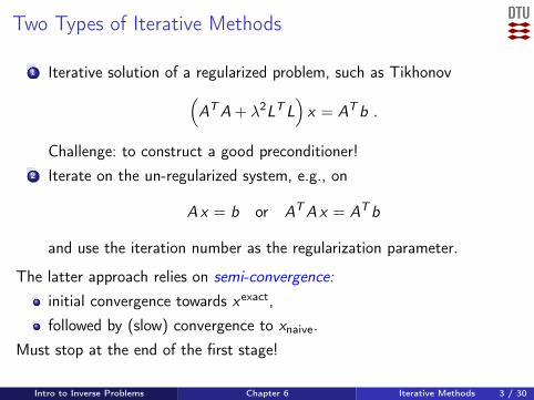
1 Iterative solution of a regularized problem, such as Tikhonov(ATA + λ2LTL

)x = ATb .

Challenge: to construct a good preconditioner!2 Iterate on the un-regularized system, e.g., on

Ax = b or ATAx = ATb

and use the iteration number as the regularization parameter.

The latter approach relies on semi-convergence:initial convergence towards xexact,followed by (slow) convergence to xnaive.

Must stop at the end of the first stage!


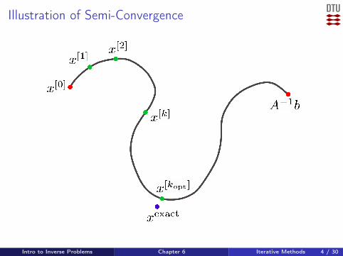
Illustration of Semi-Convergence


Landweber Iteration

A classical stationary iterative method:

x [k+1] = x [k] + ω AT (b − Ax [k]) , k = 0, 1, 2, . . .

where 0 < ω < 2 ‖ATA‖−12 = 2σ−2

1 .

Where does this come from? Consider the function

φ(x) = 12‖b − Ax‖22

associated with the least squares problem minx φ(x). It is straightforward(but perhaps a bit tedious) to show that the gradient of φ is

∇φ(x) = −AT (b − Ax).

Thus, each step in Landweber’s method is a step in the direction ofsteepest descent. See next slide for an example of iterations.


The Geometry of Landweber Iterations


SVD Analysis of Landweber’s Method

SVD analysis shows that the filter factors (see next page) are:

φ[k]i = 1− (1− ω σ2

i )k .

Let σ[k]break denote the value of σi for which f[k]i = 0.5. Then

σ[k]break

σ[2k]break

=

√1 + (1

2)12k →

√2 for k →∞.

Hence, as k increases, the breakpoint tends to be reduced by a factor√2 ≈ 1.4 each time the number of iterations k is doubled.


Landweber Filter Factors


Cimmino Iteration

Cimmino’s method is a variant of Landweber’s method, with a diagonalscaling:

x [k+1] = x [k] + ω ATD (b − Ax [k]), k = 1, 2, . . .

in which D = diag(di ) is a diagonal matrix whose elements are defined interms of the rows aTi = A(i , : ) of A as

di =

1m

1‖ai‖22

, ai 6= 0

0, ai = 0.

Landweber and Cimmino belong to a class of iterative methods calledSimultaneous Iterative Reconstruction Techniques (SIRT).


. . . and the prize for best acronym goes to “ART”

Kaczmarz’s method = algebraic reconstruction technique (ART).

Let aTi = A(i , :) = ith row of A, and bi = ith component b.

Each iteration of ART involves the following “sweep” over all rows:

x [k(0)] = x [k]

for i = 1, . . . ,m

x [k(i)] = x [k

(i−1)] +bi − aTi x

[k(i−1)]

‖ai‖22ai

endx [k+1] = x [k

(m)]

This method is not “simultaneous” because each row must be processedsequentially.In general: fast initial convergence, then slow. See next slides.


The Geometry of ART Iterations


Slow Convergence of SIRT and ART Methods

The test problem is shaw.


Projection MethodsAs an important step towards the faster Krylov subspace methods, weconsider projection methods.

Assume the columns of Wk = (w1, . . . ,wk) ∈ Rn×k form a “good basis” foran approximate regularized solution, obtained by solving

minx‖Ax − b‖2 s.t. x ∈ Wk = spanw1, . . . ,wk.

This solution takes the form

x (k) = Wk y(k), y (k) = argminy ‖(AWk) y − b‖2,

and we refer to the least squares problem ‖(AWk) y − b‖2 as the projectedproblem, because it is obtained by projecting the original problem onto thek-dimensional subspace span(w1, . . . ,wk).

If Wk = Vk then we obtain the TSVD method, and x (k) = xk

But we want to work with computationally simpler basis vectors.Intro to Inverse Problems Chapter 6 Iterative Methods 13 / 30

Computations with DCT Basis

Note that

Ak = AWk = (W Tk AT )T =

[(W TAT )T

]:,1:k

.

In the case of the discrete cosine basis, multiplication with W T isequivalent to a DCT. The algorithm takes the form:

Akhat = dct(A’)’;Akhat = Akhat(:,1:k);y = Akhat\b;xk = idct([y;zeros(n-k,1)]);

Next page:Top: solutions x (k) for k = 1, . . . , 10.Bottom: cosine basis wi , i = 1, . . . , 10.


Example Using Discrete Cosine Basis (shaw)


Symmetric Solution and DCT (phillips)Red: Using all the DCT basis vectors w1,w2,w3,w4,w5,w6, . . .

Blue: Using only the odd-numbered DCT vectors w1,w3,w5, . . .


The Krylov Subspace

The DCT basis is sometimes a good basis – but not always.

The Krylov subspace, defined as

Kk ≡ spanATb,ATAATb, (ATA)2ATb, . . . , (ATA)k−1ATb,

always adapts itself to the problem at hand! But the “naive” basis,

pi = (ATA)i−1ATb / ‖(ATA)i−1ATb‖2, i = 1, 2, . . .

are NOT useful: pi → v1 as i →∞. Use modified Gram-Schmidt:

w1 ← ATb; w1 ← w1/‖w1‖2w2 ← ATAw1; w2 ← w2 − wT

1 w2 w1; w2 ← w2/‖w2‖2w3 ← ATAw2; w3 ← w3 − wT

1 w3 w1;

w3 ← w3 − wT2 w3 w2; w3 ← w3/‖w3‖2


Comparison of basis vectors pi (blue) and wi (red)


Can We Compute x (k) Without Storing Wk?Yes – the CGLS algorithm – see next slide – computes iterates given by

x (k) = argminx ‖Ax − b‖2 s.t. x ∈ Kk .

The algorithm eventually converges to the least squares solution.

But since Kk is a good subspace for approximate regularized solutions,CGLS exhibits semi-convergence.


CGLS = Conjugate Gradients for Least Squares

The CGLS algorithm takes the following form:

x (0) = starting vector (e.g., zero)

r (0) = b − Ax (0)

d (0) = AT r (0)

for k = 1, 2, . . .

αk = ‖AT r (k−1)‖22/‖Ad (k−1)‖22x (k) = x (k−1) + αk d

(k−1)

r (k) = r (k−1) − αk Ad (k−1)

βk = ‖AT r (k)‖22/‖AT r (k−1)‖22d (k) = AT r (k) + βk d

(k−1)

end


CGLS Solutions to the Gravity Problem


CGLS Focuses on the Significant Components


And Now With Noise


Other Iterations – GMRES and RRGMRES

Sometimes difficult or inconvenient to write a matrix-free black-boxfunction for multiplication with AT . Can we avoid this?

The GMRES method for square nonsymmetric matrices is based on theKrylov subspace

Kk = spanb,Ab,A2b, . . . ,Ak−1b.

The presence of the noisy data b = bexact + e in this subspace isunfortunate: the solutions include the noise component e!

A better subspace, underlying the RRGMRES method:

~Kk = spanAb,A2 b, . . . ,Ak b.

Now the noise vector is multiplied with A (smoothing) at least once.

Symmetric matrices: use MR-II (a simplified variant).


Tomography (a Case for Iterative Methods) §7.7

Tomography is the science of computing reconstructions from projections,i.e., data obtained by integrations along rays (typically straight lines) thatpenetrate a domain Ω.

The unknown function f (t) = f (t1, t2) represents some material parameter,and the damping of a signal penetrating a part dτ of a ray at position t isproportional to the product to f (t) dτ .

The data consist of measurements of the damping of signals followingwell-defined rays through the domain Ω.


Formulation of Tomography Problem

The ith observation bi , i = 1, . . . ,m, represents the damping of a signalthat penetrates Ω along a straight line, rayi .

All the point ti on rayi are given by

ti (τ) = ti ,0 + τ di , τ ∈ R,

where ti ,0 is an arbitrary point on the ray, and di is a (unit) vector thatpoints in the direction of the ray.

The damping is proportional to the integral of the function f (t) along theray. Specifically, for the ith observation, the damping associated with theith ray is given by

bi =

∫ ∞−∞

f(ti (τ)

)dτ, i = 1, . . . ,m,

where dτ denotes the integration along the ray.


Discretization of 2D Tomography Problem

We consider a square domain Ω = [0, 1]× [0, 1].

We can discretize this problem by dividing Ω into an N × N array of pixels,and in each pixel (k, `) we assume that the function f (t) is a constant fk`:

f (t) = fk` for t1 ∈ Ik & t2 ∈ I`,

where we have defined the interval Ik = [ (k−1)/N , k/N ], k = 1, . . . ,N(and similarly for I`).

With this assumption about f (t) being piecewise constant, the expressionfor the kth measurement takes the simpler form

bi =∑

(k,`)∈rayifk` ∆L

(i)k` , ∆L

(i)k` = length of rayi in pixel (k, `)

for i = 1, . . . ,m.


Illustration of Discretization

-

6

t1

t2

""""""""""""""""""""

rayi :ti (τ) = ti ,0 + τ di

I1 I2 I3 I4 I5 I6

I1

I2

I3

I4

I5

I6

f11

f12 f22 f32

f33 f43

f44 f54 f64

f65


Arriving at the System of Linear Equations

The above equation is, in fact, a system of linear equations in the N2

unknowns fk`. We introduce the vector x of length n = N2 whose elementsare the (unknown) function values fk`:

x` = fk`, ` = (k − 1)N + `.

This corresponds to stacking the columns of the N × N matrix F .Moreover we organize the measurements bi into a vector b.

There is clearly a linear relationship between the data bk and the unknownsin the vector x , meaning that we can always write

bi =n∑

j=1

aij xj , i = 1, . . . ,m.

This is a system of linear equations Ax = b with an m × n matrix.


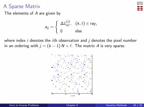
A Sparse MatrixThe elements of A are given by

aij =

∆L

(i)k` , (k , `) ∈ rayi

0 else

where index i denotes the ith observation and j denotes the pixel numberin an ordering with j = (k − 1)N + `. The matrix A is very sparse.


Documents

ProblemsofVaryingSize - Technical University of Denmarkpcha/DIP/chap6.pdfProblemsofVaryingSize Small-scaleproblems “anythinggoes, ... Hence,aspk increases,thebreakpointtendstobereducedbyafactor